Generalized single-parameter aging tests and their application to glycerol

Abstract

Physical aging of glycerol following temperature jumps is studied by dielectric spectroscopy at temperatures just below the glass transition temperature. The data are analyzed using two single-parameter aging tests developed by Hecksher et al. [J. Chem. Phys. 142, 241103 (2015)]. We generalize these tests to include jumps ending at different temperatures. Moreover, four times larger jumps than previously are studied. The single-parameter aging tests are here for the first time applied to a hydrogen-bonded liquid. We conclude that glycerol obeys single-parameter aging to a good approximation.

I Introduction

Supercooled liquids are liquids cooled with a cooling rate fast enough to avoid crystallizationCotterill (1985). As the glass transition is approached the liquid becomes more and more viscous, and at the glass transition temperature ($T_{g}$) the molecules effectively stop moving on the experimental time scaleBrawer (1985). Supercooled liquids are often studied using linear response experiments as for example dielectric spectroscopy, where a change in the electric field (a perturbation) leads to a change in polarization (a response). The perturbation is in this case usually small in order to ensure that the response depends linearly on the applied perturbation, and the measured response function is connected to the dynamics in equilibrium via the fluctuation dissipation theorem. In contrast to linear response experiments, aging is the response following a large perturbation, where the liquid is brought out of equilibrium, and the study of aging is a study of how the properties of a system change over time as it relaxes toward equilibriumScherer (1986). Aging is highly non-linear since the relaxation rate itself changes as the liquid equilibrates. Most aging studies, including the work presented in this paper, are studies of how the system responds to a change in temperature. The experiments are performed close to and below the glass transition temperature, where aging takes place on time scales that are slow enough to be measurable, yet fast enough to follow all (or a substantial part) of the relaxation towards equilibrium. Close to the glass transition temperature, the rate of the structural relaxation depends strongly on temperature, and aging is non-linear even for fairly small temperature steps. For a jump down in temperature the structural relaxation becomes slower as time evolves, whereas for an jump up in temperature the rate of structural relaxation increases as time evolves.

The study of aging has a very practical root. The out-of-equilibrium nature of glasses has the consequence that the properties of all glassy materials age, even if it is sometimes very slow. The standard formalism for describing this was set out by Narayanaswamy, an engineer at Ford Motor Company who needed a method for predicting how the frozen-in stresses in a wind-shield depend on the glass’ thermal history Narayanaswamy (1971). Inspired by Tool, Narayanaswamy introduced a single-parameter aging assumption in terms of a fictive temperatureHecksher et al. (2015). Today this is referred to as the Tool-Narayanaswamy (TN) formalism. Besides the obvious importance for application of glasses, aging experiments have the potential to yield new information about fundamental outstanding questions regarding the equilibrium relaxation (e.g. Ref. Niss, 2017).

The analysis in this paper is based on the TN aging formalism Tool (1946); Narayanaswamy (1971); Scherer (1986); Dyre (2015). The TN-formalism interprets aging in terms of a material time $\xi$. The material time may be thought of as a time measured on a clock with a clock rate that changes as the system ages. The material time is defined from the clock rate $\gamma(t)$ byNarayanaswamy (1971); Dyre (2015)

$$d\xi=\gamma(t)dt.$$ (1)

Narayanaswamy’s idea was that linearity of the response is restored using the material time implying that the non-linear aging can be described using a linear convolution integral. The central hypothesis of single-parameter aging is that the clock-rate, $\gamma(t)$, depends only on one structural parameter, and that this parameter also controls the measured quantity.

Hecksher et al. 2015Hecksher et al. (2015) derived two tests of the single-parameter assumption, which are used and further developed below. The conceptual starting point of the tests is an “ideal aging experiment” in which aging is measured from equilibrium to a new equilibrium after an “instantaneous” jump in temperature. In Sec. II, we discuss how to perform an experiment that comes close to the ideal aging experiment. The tests from 2015 have the advantage that it is not necessary to calculate the material time explicitly in order to test for single-parameter aging. The tests are in these respects similar to tests we developed in 2010 Hecksher et al. (2010) and 2017 Niss (2017). The single-parameter aging tests can only be applied for simple jumps in temperature, whereas other applications of the TN formalism may be used on more advanced thermal histories. However, usually other applications of the TN formalism assumes that the shape of the relaxation curve can be described by, e.g., a streched exponential and some functional form for how the clock rate depends on temperature and fictive temperature $\gamma=\gamma(T,T_{f})$.

The unique feature of one of the 2015-tests is that if a liquid obeys single-parameter aging, then one relaxation curve can be used to predict other relaxation curves. In particular, this implies that it is possible to predict linear relaxation curves from the non-linear curves without evaluating the material time. The linear response to a temperature jump is not easy to measure because it requires a very small temperature change. In this paper we extend the tests and procedures from Hecksher et al. 2015 to work also for jumps with different final temperature.

Hecksher et al.Hecksher et al. (2015) concluded that the three van der Waals liquids investigated all conform to single-parameter aging to a good approximation. It is of interest to test whether hydrogen-bonded liquids also exhibit single-parameter aging. The difference between van der Waals bonded liquids and hydrogen-bonded liquids is, in particular, important in relation to the isomorph theoryGnan et al. (2009); Dyre (2014), which predicts that van der Waals liquids have simple behavior along isochrones, e.g., isochronal superpositionTölle (2001); Roland et al. (2003); Pawlus et al. (2003); Ngai et al. (2005); Roland et al. (2008), whereas no predictions are given for hydrogen-bonded liquids. Investigations of both types of liquids are particularly relevant following the recent development of isomorph theory of physical agingDyre (2018).

The TN-formalism was originally developed for oxide glasses, which are covalently bonded systems, i.e., have strongly directional bonds. With that in mind it would not be surprising to find that the TN-formalism works also for hydrogen-bonding systems. On the other hand, the single-parameter tests we use are performed on high-precision data and the tests are developed to have no free fitting parameters. So far we have only performed these high precision parameter-free tests on van der Waals bonded liquids Hecksher et al. (2010, 2015); Niss (2017), but in this paper we present data and tests on the hydrogen bonding liquid, glycerol. Physical aging of glycerol has been studied before, e.g., in Refs.  Moynihan et al., 1991; Fujimori et al., 1992; Miller and MacPhail, 1997a, b; Simon and McKenna, 1997; Lunkenheimer et al., 2005, with some of them showing that glycerol comply to the TN model. Other alcohols were also shown to comply to the TN model Wang et al. (2008). All these investigations, however, involve one or more free parameters.

Glycerol (propane-1,2,3-triol) is a small molecule with three hydroxyl groups. It is the molecular liquid most often studied in glassy dynamics, e.g. Refs. Gibson and Giauque, 1923; Wang and Wright, 1971; Schiener et al., 1996; Berthier et al., 2005; Pezeril et al., 2009; Albert et al., 2016, and it is of importance in technology, notably due to its cryoprotectant properties Salt (1958); Dashnau et al. (2006); Li et al. (2008). For these reasons glycerol is sometimes referred to as the archetypical glass former. Yet, it is also known that glycerol supports the formation of a 3D hydrogen-bonded network penetrating the bulk liquidTowey et al. (2011), and it was recently shown that glycerol exihibits a low-frequency mode in the mechanical relaxation spectra Jensen et al. (2018). Thus there is dynamics on a slower time scale than the main relaxation – possibly due to the hydrogen bonding network. This could influence the structural state of the liquid and thereby the number of parameters involved in physical aging.

Section II gives an overview over the experimental details. Section III presents the data and initial data treatment. Generalized single-parameter aging tests are derived in Sec. IV, where also the results of the tests are shown. Section V discusses the generalized single-parameter aging tests and their ability to predict jumps, and our results are discussed in light of the isomorph theory.

II Experimental protocol and details

II.1 General considerations on the protocol

We ideally want to perform a temperature jump instantaneously. Since this is not possible, we instead aim for the time it takes to change the temperature and reach thermal equilibrium throughout the sample, to be much smaller than the structural relaxation time of the liquid. In this case we may assume that no structural changes takes place during the temperature jump, and that the liquid experiences the jump as “instantaneous”.

In order to study a full aging curve, it is important to apply the perturbation at the right temperature. If the temperature is too far below $T_{g}$, the liquid will not reach equilibrium on the experimental time scale, because of the strong temperature dependence of the structural relaxation time. On the other hand, if the perturbation is applied at a temperature too far above $T_{g}$, the liquid will come into equilibrium too fast for the aging to be measureble. This, of course, depends on how fast one can measure. If the relaxation time is close to the time it takes to make a measurement, structural relaxation will occur during the measurement. This leaves only a small temperature interval where conditions are optimal.

With our equiliment we can perform the temperature jump in a few seconds. The starting temperature is a few degrees below the conventional glass transition temperature (at which the relaxation time is 100 sDebenedetti (1996)). At the temperatures studied the relaxation time of the liquid is between 200 s and 23 hours. Table 1 shows relaxation time for each temperature along with the annealing time for each jump which ranges from a couple of hours to more than 20 days.

End temp.	Jump	Annealing time	$\tau_{eq}$ at end temp.
184 K	180 K $\rightarrow$ 184 K	$\log(t/s)=3.7$ $\approx 1.4$ hours	$\log(\tau_{eq}/s)=2.3$ $\approx 3$ min
	176 K $\rightarrow$ 184 K	$\log(t/s)=3.9$ $\approx 2.2$ hours
180 K	184 K $\rightarrow$ 180 K	$\log(t/s)=4.8$ $\approx 18$ hours	$\log(\tau_{eq}/s)=3.6$ $\approx 66$ min
	178 K $\rightarrow$ 180 K	$\log(t/s)=4.8$ $\approx 18$ hours
	176 K $\rightarrow$ 180 K	$\log(t/s)=5.0$ $\approx 30$ hours
178 K	180 K $\rightarrow$ 178 K	$\log(t/s)=5.5$ $\approx 90$ hours	$\log(\tau_{eq}/s)=4.3$ $\approx 5.5$ hours
176 K	184 K $\rightarrow$ 176 K	$\log(t/s)=6.3$ $\approx 23$ days	$\log(\tau_{eq}/s)=4.9$ $\approx 23$ hours
	180 K $\rightarrow$ 176 K	$\log(t/s)=6.2$ $\approx 18$ days

Table 1: Times. The annealing time for each jump ranges from a couple of hours to more than 20 days. The relaxation time at the end temperature $\tau_{eq}$ is found from Eq. (8).

II.2 Temperature control

In order to change the temperature fast, we use a specially designed microregulator as sample cellHecksher et al. (2010); Niss et al. (2012); Hecksher et al. (2015); Niss (2017). The microregulator is placed in a main cryostatIgarashi et al. (2008a). The microregulator keeps temperature fluctuations below 100 $\mu K$ and the characteristic thermal equilibrium time is 2 s. More details are given in Ref. Hecksher et al., 2010. In the studied temperature range the time it takes to change temperature is below the relaxation time of the liquid. We can therefore assume that little structural relaxation takes place in the liquid during the temperature change (with the possible exception of jumps starting at 184 K, where the relaxation time is only 100 times longer that the thermal equilibrium time).

II.3 Permitivity – the monitored property

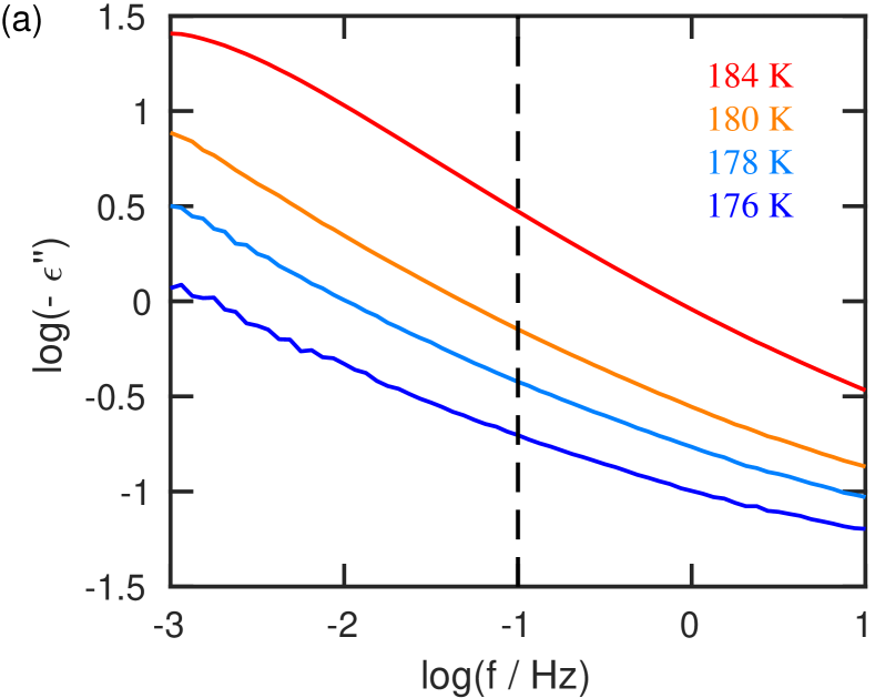
An aging experiment monitors how a selected quantity evolves over time. In this work we monitor the dielectric permitivity at a fixed frequency. The dielectric signal is a useful probe because it can be measured with high precision and has therefore been used to monitor aging in several earlier works e.g. Schlosser and Schönhals Schlosser and Schönhals (1991), Loidl and Lunkenheimer et al.Schneider et al. (2000); Lunkenheimer et al. (2005, 2006); Wehn et al. (2007), Richert et al.Richert Ranko et al. (2013), Alegría et al.Alegría et al. (1995); Alegría A. et al. (1997); Goitiandia and Alegría (2004), and Cangialosi et al.Cangialosi et al. (2005). We use dielectric spectroscopy with a parallel plate capacitor with diameter 10 mm and liquid layer of 50 $\mu m$. The electrical measurement equipment is described in Ref. Igarashi et al., 2008b. In order to perform the measurements fast, a single measuring frequency is chosen, at which the dielectric loss is measured as a function of time. The frequency is chosen to be on the high-frequency flank of the $\alpha$-peak. Figure 1 (a) shows the dielectric equilibrium spectra at the temperatures where the jumps are performed, marking the frequency used for monitoring 0.1 Hz, which corresponds to a acquisition time of 20 s. For most measurements, we can assume that no structural changes take place in the liquid during the measurement; however, for the measurements starting at the highest temperature (184 K) where the equilibrium relaxation time is just 200 s, some structural relaxation may occur during the first few measurements.

Figure 1: Raw data. (a) The dielectric loss as a function of frequency at equilibrium at the temperatures the jumps are performed between. The dashed black line marks the frequency 0.1 Hz used for monitoring aging. (b) The temperature and the measured quantity ($\log(-\varepsilon^{\prime\prime}(f=0.1\text{Hz}))$) as functions of time. (c) The jumps on a logarithmic time scale. The data have been averaged in order to reduce noise as described in the text.

II.4 Sample

Glycerol was acquired from Fluka and placed in an desiccator for 18 h before the experiment. In order to prevent the liquid taking up water from the surrounding air, the cryostat was heated to 300 K before use. It was then flushed with liquid nitrogen, after which the microregulator with sample was placed in the cryostat and the temperature was lowered to 245 K (well below the melting temperature of water).

III Measurements and initial data analysis

III.1 Protocol and raw data

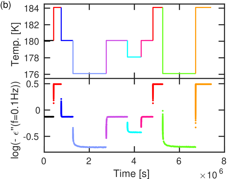
The measuring protocol is the following: The liquid is brought into equilibrium at the starting temperature 180 K (a few degrees below $T_{g}\approx 185$ K). We spent 35 days ($\log(t_{anneal}/s)=6.5$) for annealing the sample; equilibrium spectra were taken at different temperatures while cooling to estimate the right starting temperature. A jump in temperature is performed, and the liquid is monitored until equilibrium is established. A new jump is then performed. During the jumps the dielectric loss at the measuring frequency is monitored as a function of time ($\log(-\varepsilon^{\prime\prime}(f=0.1\text{Hz},t))$). The jump magnitudes are 2 K, 4 K, and 8 K.

The temperature protocol and the raw data of the aging measurements are seen in Fig. 1 (b), where each color represents a jump. Throughout the paper, reddish color tones are used for up jumps and bluish color tones are used for down jumps. The jump from 180 K to 184 K is performed twice, which served as a check of reproducibility, but only the first jump is used in the further data treatment. The total time of the measurement series is several months. The data are available on Glass and Time’s data repository (http://glass.ruc.dk).

III.2 Initial data analysis

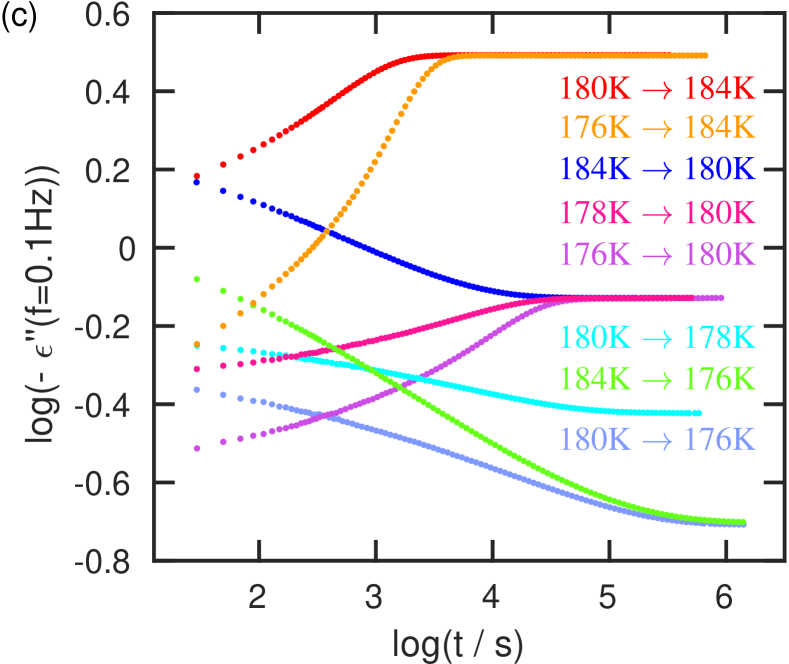
Figure 1 (c) shows the data on a logarithmic time scale. The data are here averaged in order to reduce noise, which is done on a logarithmic scale by proceeding as follows. The first 15 raw data points are kept, then the $\log(time)$-scale are divided into 90 equal sized intervals over which the raw data are averaged. Figure 1 (c) demonstrates that different jumps ending at the same temperature reach the same equilibrium value. It is on the other hand not clear in this figure that jumps starting at the same temperature have the same initial value. This is due to the instantanous contribution to the aging. Note that same size up and down jumps are not symmetric, which is due to the non-linearity seen even for small jumps.

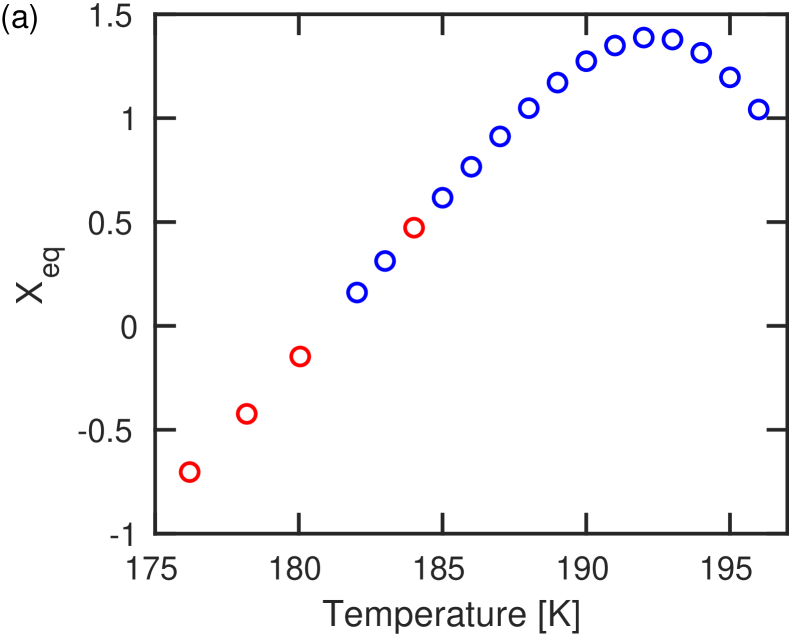
For the further data treatment some notation is now introduced. The jump is performed from the starting temperature $T_{start}$ and ends at the temperature $T_{end}$. The measured time-dependent quantity is denoted $X(t)=\log(-\varepsilon^{\prime\prime}(f=0.1\text{Hz},t))$. The jump starts at $t=0$ and the starting value of the measured quantity $X(0)$ is the equilibrium value of the measured quantity at $T_{start}$. When the liquid is in equilibrium at $T_{end}$ as $t\rightarrow\infty$, the measured quantity is $X_{eq}$. Figure 2 (a) shows $X_{eq}$ as a function of temperature. The time-dependent distance to equilibrium at $T_{end}$ is denoted $\Delta X(t)=X(t)-X_{eq}$. $\Delta X(0)$ is the total change of the measured quantity from $T_{start}$ to $T_{end}$. The definition of $\Delta X(t)$ is a generalization of other concepts that quantify the departure from equilibrium, e.g., Kovacs’ expression in terms of volume $\delta(t)=(V(t)-V_{\infty})/V_{\infty}$Kovacs (1963).

Figure 2: Quantities used in the data analysis to perform the single-parameter tests. (a) The measured quantity ($\log(-\varepsilon^{\prime\prime}(f=0.1\text{Hz},t))$) at equilibrium at the final temperature ($X_{eq}$) as a function of temperature. The red circles indicate the four temperatures between which jumps are performed. The peak appearing between 190 K and 195 K is due to the $\alpha$-peak moving across the measuring frequency. (b) The normalized relaxation functions as functions of time for all jumps.

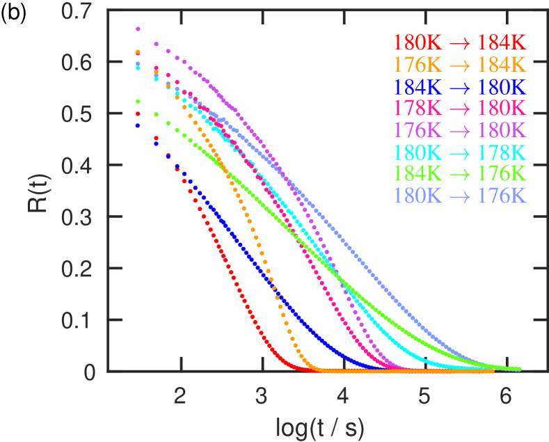
The normalized relaxation function $R(t)$ is defined as the time-dependent distance to equilibrium over the overall change from start to end of the measured quantityNarayanaswamy (1971); Scherer (1986)

$$R(t)=\frac{\Delta X(t)}{\Delta X(0)}$$ (2)

It is seen that $R(0)=1$ and that $R(t)\rightarrow 0$ as $t\rightarrow\infty$. Figure 2 (b) shows $R(t)$ for all jumps. According to the TN formalism $R(t)$ is a unique function of the material time $\xi$Scherer (1986).

IV Generalized single-parameter aging tests

Two single-parameter aging tests were derived by Hecksher et al. 2015Hecksher et al. (2015) for jumps ending at the same temperature. In this investigation we study jumps to different temperatures, and the single-parameter aging tests are therefore generalized below.

According to the single-parameter assumption, both the measured quantity $X(t)$ and the clock rate $\gamma(t)$ are controlled by the same parameter $Q(t)$. Hecksher et al.Hecksher et al. (2015) assumed that the temperature jumps are so small that it is reasonable to Taylor expand both $X(t)$ and $\ln\gamma(t)$ to the first order in $Q(t)$: $\Delta X(t)\cong c_{1}\Delta Q(t)$ and $\Delta\ln\gamma(t)\cong c_{2}\Delta Q(t)$, where $c_{1}$ and $c_{2}$ are constants and $\Delta X(t)$, $\Delta Q(t)$, and $\Delta\ln\gamma(t)$ defines the time-dependent distance to equilibrium for respectively $X(t)$, $Q(t)$, and $\ln\gamma(t)$. Eliminating $\Delta Q(t)$ in the equations gives $\ln\gamma(t)=\ln\gamma_{eq}+\Delta X(t)/X_{const}$, where $X_{const}=c_{1}/c_{2}$. Using the definition of $R(t)$ (Eq. (2)) gives

$$\gamma(t)=\gamma_{eq}\exp\left(\frac{\Delta X(0)}{X_{const}}R(t)\right)$$ (3)

As expected $\gamma(t)\rightarrow\gamma_{eq}$ as $t\rightarrow\infty$ because $R(t)\rightarrow 0$. Hecksher et al.Hecksher et al. (2015) derived the following expression for the time-derivative of $R$ from the TN-formalism

$$\dot{R}=-F(R)\gamma(t)$$ (4)

where $F(R)$ is a unique function of $R$, i.e., independent of start and end temperature. Since $R(t)$ goes from 1 to 0, $\dot{R}<0$, and $F(R)>0$ per definition.. Inserting the expression for $\gamma$ (Eq. (3)) and rearranging leads to

$$-\frac{\dot{R}}{\gamma_{eq}}\exp\left(-\frac{\Delta X(0)}{X_{const}}R(t)\right)=F(R)$$ (5)

from which the two generalized tests are derived in the following sections.

IV.1 Test 1 - Predicting general jumps from knowledge of a single jump

If single-parameter aging is obeyed, it is possible to predict the relaxation function for one jump from the relaxation function of another jump. In the following we use subscripts 1 and 2 to distinguish between the known (measured) relaxation function – jump 1 – and the predicted relaxation function – jump 2. From one jump relaxation function $R_{1}(t)$ and its inverse function $t_{1}(R)$, we derive a method for determining $t_{2}(R)$ for a different jump $R_{2}(t)$ using Eq. (5).

At times $t_{1}^{*}(R)$ and $t_{2}^{*}(R)$ where the value of the relaxation functions are the same ($R=R_{1}=R_{2}$), Eq. (5) implies

$$-\frac{dR_{1}}{dt_{1}^{*}}\cdot\frac{1}{\gamma_{eq,1}}\cdot\exp\left(-\frac{\Delta X_{1}(0)}{X_{const}}R_{1}(t_{1}^{*})\right)=-\frac{dR_{2}}{dt_{2}^{*}}\cdot\frac{1}{\gamma_{eq,2}}\cdot\exp\left(-\frac{\Delta X_{2}(0)}{X_{const}}R_{2}(t_{2}^{*})\right)\,.$$ (6)

For time increments $dt_{1}^{*}$ and $dt_{2}^{*}$ leading to identical changes $dR_{1}=dR_{2}$ we can write Eq. (6) using the premise that $R_{1}(t_{1}^{*})=R_{2}(t_{2}^{*})$ to give

$$dt_{2}^{*}=\frac{\gamma_{eq,1}}{\gamma_{eq,2}}\cdot\exp\left(\frac{\Delta X_{1}(0)-\Delta X_{2}(0)}{X_{const}}R_{1}(t_{1}^{*})\right)dt_{1}^{*}\,.$$ (7)

Integrating this leads to (assuming that both jumps are initiated at time zero)

$$t_{2}=\int_{0}^{t_{2}}dt_{2}^{*}=\frac{\gamma_{eq,1}}{\gamma_{eq,2}}\int_{0}^{t_{1}}\exp\left(\frac{\Delta X_{1}(0)-\Delta X_{2}(0)}{X_{const}}R_{1}(t_{1}^{*})\right)dt_{1}^{*}\,,$$ (8)

which determines $t_{2}(t_{1})=t_{2}(t_{1}(R))=t_{2}(R)$, predicting the inverse function $R_{2}(t)$.

In practice, we do not need to do an inversion. The procedure is to transform a discrete set of measured data points, a time vector ${\bf t}_{1}=(t_{1}^{1},t_{1}^{2},\ldots,t_{1}^{n})$ and the corresponding relaxation vector ${\bf R}_{1}=(R_{1}^{1},R_{1}^{2},\ldots,R_{1}^{n})$) to a new time vector ${\bf t}_{2}=(t_{2}^{1},t_{2}^{2},\ldots,t_{2}^{n})$ corresponding to the measured ${\bf R}_{1}$ points. Plotting $({\bf t}_{2},{\bf R}_{1})$ should then coincide with $R_{2}$, which can be tested by a separate measurement.

For jumps ending at the same temperature Eq. (8) reduces to

$$t_{2}=\int_{0}^{t_{1}}\exp\left(\frac{\Delta X_{1}(0)-\Delta X_{2}(0)}{X_{const}}R_{1}(t_{1}^{*})\right)dt_{1}^{*}\,,$$ (9)

which is the equation used in Hecksher et al.Hecksher et al. (2015).

The new generalized test has the disadvantage that one needs to know the equilibrium clockrate $\gamma_{eq}$. By assuming an internal clockHecksher et al. (2010); Jakobsen et al. (2012), i.e., that the clock rates from dielectric spectroscopy and structural relaxation are proportional, one may define the clock rate at $T_{end}$ ($\gamma_{eq}$) as the dielectric inverse relaxation time ($\gamma_{eq}=1/\tau$), where the relaxation time is determined from the maximum frequency at the $\alpha$-peak ($f_{m}$) as $\tau=1/(2\pi f_{m})$. At the temperatures where jumps are performed, we cannot determine $\tau$ directly, since the $\alpha$-peak is outside the available frequency range (see Fig. 1 (a)). One may find $\gamma_{eq}$ using an extrapolation or determine $\gamma_{eq}$ in another way. Below we let the constant $\frac{\gamma_{eq,1}}{\gamma_{eq,2}}$ in Eq. (8) be a free parameter to find the $\gamma_{eq}$ that gives the best prediction (which is very close to the prediction using a Vogel-Fulcher-Tammann (VFT) extrapolation as shown in Fig. 4).

The constant $X_{const}$ was identified using two jumps to the same temperature; the down jump 184 K to 180 K and the up jump 176 K to 180 K. A fit is made using Eq. (9) to find the $X_{const}$ that gives the best prediction of one jump from the other. This gives $X_{const}=0.16$, which was used for all jumps.

The result of the test is shown in Fig. 3. The up jump 176 K to 180 K (Fig. 3 (a)) is used to predict the other jumps. The predictions are good, however with deviations in particular at short times, similar to those observed for the van der Waals liquids tested in Hecksher et al. 2015Hecksher et al. (2015). The 8 K jumps have larger deviations than the smaller jumps, however, still not more dramatic than results on van der Waals liquidsHecksher et al. (2015). Since we use a first-order Taylor expansion in the derivation of the test, it is not surprising that the predictions are slightly worse for large temperature jumps.

Figure 3: Test 1. Prediction of jumps based on the jump 176 K to 180 K (shown in (a)). In (b), (c), and (d) circles are data and black lines are predictions. The up jump 176 K to 180 K and the down jump 184 K to 180 K were used to find $X_{const}$ (indicated by * in legend), while $\gamma_{eq}(T)$ was a fitting parameter the consistency of which with equilibrium dynamics is checked in Fig. 4. The predictions are good, however, with deviations in particular at short times. It is also seen that the predictions are slightly worse for the largest jumps as well as for the down jumps starting at the highest temperatures.

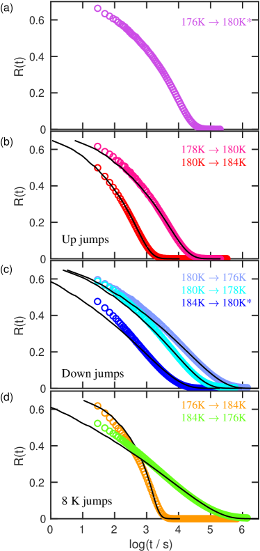
Note that the two down jumps starting at 184 K both have significant deviations at short times. This may be related to the relatively fast relaxation time at this starting temperature, and structural relaxation may have occured during the jump and during the first measurements making these jumps less ideal in the sense defined earlier.

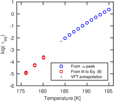
Figure 4 shows $\gamma_{eq}$ as a function of temperature found from the free parameter $\gamma_{eq,1}/\gamma_{eq,2}$ in Eq. (8). To determine $\gamma_{eq}$ for each temperature, we used a value of $\gamma_{eq}$ at 184 K found from a VFT-fit to higher temperature data. Different jumps to the different temperatures give a slightly different value, but this is barely visible in the figure. The values found are reasonable, but vary slighty from the predictions of $\gamma_{eq}$ from VFT. This supports the internal clock hypothesis, i.e., that the clock rates from dielectric spectroscopy and structural relaxation are proportional. This is in line with the result in Ref. Lunkenheimer et al., 2005. The values of $\gamma_{eq}$ are given in Table 2.

Figure 4: The clock rate at equilibrium at the end temperature ($\gamma_{eq}$) found from equilibrium spectra (blue circles). The red circles are determined from the free parameter $\gamma_{eq,1}/\gamma_{eq,2}$ in Eq. (8). Since we have two jumps to 180 K and to 176 K, this results in two values of $\gamma_{eq}$ at these temperatures. However, the difference is barely visible. The black dots are the predictions from the VFT-fit.

Temperature	$\log(\gamma_{eq})$ from Eq. (8)	Average $\log(\gamma_{eq})$ from Eq. (8)	$\log(\gamma_{eq})$ from VFT
184 K			-2.28
180 K	-3.62	-3.64	-3.50
	-3.67
178 K	-4.27	-4.29	-4.16
	-4.31
176 K	-4.92	-4.92	-4.88
	-4.96
	-4.89
	-4.93

Table 2: The equilibrium clock rate at the end temperature $\gamma_{eq}$ determined from Eq. (8). To invert $\gamma_{eq,1}/\gamma_{eq,2}$ to $\gamma_{eq}$, we first used the value of $\gamma_{eq}$ at 184 K found from a VFT-fit to estimate $\gamma_{eq}$ at 180 K (resulting in two values because there are two jumps to 184 K). The estimated $\gamma_{eq}$ at 180 K are then used to determine $\gamma_{eq}$ at 178 K and 176 K. Different jumps to the same temperature give a slightly different value of $\gamma_{eq}$. Furthermore, values found from extrapolations of VFT-fit are given.

IV.2 Test 2 - Unique function of $R$

Taking the logarithm of Eq. (5) leads to (remember that $\dot{R}<0$)

$$\ln\left(-\frac{\dot{R}}{\gamma_{eq}}\right)-\frac{\Delta X(0)}{X_{const}}R=\ln(F(R))$$ (10)

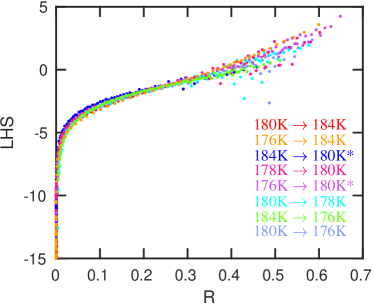
Since $F(R)$ is a unique function of $R$ if single-parameter aging applies, the left hand side of Eq. (10) (denoted LHS following Hecksher et al. 2015Hecksher et al. (2015)) is also a unique function of $R$. This means that LHS plotted against $R$ for the different jumps collapse onto a master curve if a single parameter controls both $X(t)$ and $\gamma(t)$. $\gamma_{eq}$ found from Test 1 is used. For each temperature the found values of $\gamma_{eq}$ is now averaged, so that each temperature has a fixed $\gamma_{eq}$.

Figure 5 shows that the data collapse onto a master curve. As also seen with test 1, deviations are observed in particular at short times (large $R$).

Figure 5: Test 2. The left hand side of Eq. (10) (LHS) plotted against $R$ for all jumps. If the liquid obeys single-parameter aging, the data are predicted to collapse onto a master curve which is seen to apply to a good approximation.

V Discussion & conclusion

V.1 How to test the single-parameter assumption

The data analysis emphasizes that measurements must be precise to allow for direct tests of single-parameter aging. It is important that the liquid is in equilibrium at the starting temperature. The liquid does not have to reach full equilibrium if one knows the correct $X_{eq}$; i.e., where it should end. Our analysis revealed that it is crucial to have the correct $X_{eq}$. Performing an up jump from the glassy state makes it possible to monitor a full relaxation curve where both the plateau in the beginning and the end are present. For this reason it is recommended to use such a jump for predicting other jumps.

Test 1, which is used to predict the curves, is the most sensitive test. By using test 1 it is possible to find $\gamma_{eq}$ at temperatures where the peak is not present in the dielectric equilibrium spectrum. If one knows $\gamma_{eq}$ (for example by an extrapolation from higher temperatures), an advantage of test 1 is that if a liquid obeys single-parameter aging, one can use Eq. (8) to predict relaxation curves. It is necessary to perform two jumps (preferably to the same temperature) to identify $X_{const}$. Other jumps can then be predicted knowing the clock rate at the end temperature ($\gamma_{eq}$), the measured quantity at the starting temperature ($X(0)$), and the measured quantity at the end temperature ($X_{eq}$). $\Delta X(0)=X(0)-X_{eq}$ determines the shape of the relaxation, while $\gamma_{eq}$ determines the position of the relaxation. This is of course also limited to small jumps, and possible only in the same temperature range as the jumps are performed in.

V.2 The scope of single-parameter aging

Hecksher et al. 2015Hecksher et al. (2015) demonstrated single-parameter aging for three different van der Waals liquids. In the present investigation the tests have for the first time been applied to a hydrogen-bonded liquid. The comparison of hydrogen-bonded liquids and van der Waals bonded liquids is interesting in view of the isomorph theory, which states that R-simple liquids have simple behavior along isochronesGnan et al. (2009); Dyre (2014). Van der Waals bonded liquids are expected to be R-simple, whereas hydrogen-bonded liquids are not. The isomorph theory was suggested a decade ago, and since then it has been tested in a number of investigations, e.g., Refs.  Gundermann et al., 2011; Roed et al., 2013; Xiao et al., 2015; Roed et al., 2015; Adrjanowicz et al., 2016; Hansen et al., 2018. Earlier investigations of density scalingDreyfus et al. (2003); Alba-Simionesco et al. (2004); Casalini and Roland (2004); Roland et al. (2005) and isochronal superpositionTölle (2001); Roland et al. (2003); Pawlus et al. (2003); Ngai et al. (2005); Roland et al. (2008) also follow the predictions of the isomorph theory. The understanding of aging in computer simulation was connected to isomorph theory already in 2010 Gnan et al. (2010), and recently experimental results Niss (2017) and aging theory Dyre (2018) were also analyzed and developed in the framework of isomorph theory. Based on these earlier works we expected that single-parameter aging might not work for a hydrogen-bonding network-forming system like glycerol. However, based on the tests presented above we find that single-parameter aging works to a good approximation also for glycerol. The quantitative agreement with the predictions from the single-parameter aging found for glycerol is, in fact, similar to that found for three van der Waals bonding liquids in Ref. Hecksher et al., 2015. This finding suggests that single-parameter aging works for a wider range of systems than those complying to isomorph theory, which also means that single-parameter aging needs to be understood in a more general theoretical framework.

The tests work well also for the large jumps (4 K and 8 K), while they previously were applied only to jumps of maximum 2 KHecksher et al. (2015). Note that a jump of a certain temperature span corresponds to different spans in $\gamma_{eq}$ for different liquids. In particular the difference in fragility between hydrogen-bonded liquids and van der Waals bonded liquids means that temperature jumps of equal sizes corresponds to a larger change of $\gamma_{eq}$ for the van der Waals bonded liquids. The 8 K jump of glycerol corresponds to $\Delta\log\gamma_{eq}\approx 2.6$, while $\Delta\log\gamma_{eq}\approx 0.3$ to 0.8 for the previously tested jumps on van der Waals liquids (the total span of $\gamma_{eq}$ for the used up and down jump is $\Delta\log\gamma_{eq}\approx 0.7$ to 1.5). This implies that also with respect to $\Delta\log\gamma_{eq}$ the jumps studied here are larger than tested before. For the 8 K jumps single-parameter aging may begin to break down, but this is not surprising since a first-order Taylor expansion is used in the derivation of the tests. For future works higher-order Taylor expansions could be introduced into the tests.

VI Acknowledgement

L. A. R. and K. N. want to thank Independent Research Fund Denmark (Sapere Aude: Starting Grant) and Danish National Research Foundation’s Grant No. DNRF61 for supporting this work. T. H. and J. C. D. are supported by the VILLUM Foundation’s Matter grant (16515).

References

- Cotterill (1985) R. Cotterill, The Cambridge guide to the material world (Cambridge University Press, Cambridge, 1985), ISBN 0521246407.
- Brawer (1985) S. Brawer, Relaxation in viscous liquids and glasses, review of phenomenology, molecular dynamics simulations, and theoretical treatment (American Ceramic Society, Columbus, Ohio, 1985), ISBN 0916094685.
- Scherer (1986) G. W. Scherer, Relaxation in glass and composites (Wiley, New York, 1986), ISBN 0471819913.
- Narayanaswamy (1971) O. S. Narayanaswamy, J. Am. Ceram. Soc. 54, 491 (1971).
- Niss (2017) K. Niss, Phys. Rev. Lett. 119, 115703 (2017).
- Tool (1946) A. Q. Tool, J. Am. Ceram. Soc. 29, 240 (1946).
- Dyre (2015) J. C. Dyre, J. Chem. Phys. 143, 114507 (2015).
- Hecksher et al. (2015) T. Hecksher, N. B. Olsen, and J. C. Dyre, J. Chem. Phys. 142, 241103 (2015).
- Hecksher et al. (2010) T. Hecksher, N. B. Olsen, K. Niss, and J. C. Dyre, J. Chem. Phys. 133, 174514 (2010).
- Gnan et al. (2009) N. Gnan, T. B. Schrøder, U. R. Pedersen, N. P. Bailey, and J. C. Dyre, J. Chem. Phys. 131, 234504 (2009).
- Dyre (2014) J. C. Dyre, J. Phys. Chem. B 118, 10007 (2014).
- Dyre (2018) J. C. Dyre, J. Chem. Phys. 148, 154502 (2018).
- Moynihan et al. (1991) C. Moynihan, S. Crichton, and S. Opalka, J. Non-Cryst. Solids 131, 420 (1991).
- Fujimori et al. (1992) H. Fujimori, Y. Adachi, and M. Oguni, Phys. Rev. B 46, 14501 (1992).
- Miller and MacPhail (1997a) R. S. Miller and R. A. MacPhail, J. Phys. Chem. B 101, 8635 (1997a).
- Miller and MacPhail (1997b) R. S. Miller and R. A. MacPhail, J. Chem. Phys. 106, 3393 (1997b).
- Simon and McKenna (1997) S. L. Simon and G. B. McKenna, J. Chem. Phys. 107, 8678 (1997).
- Lunkenheimer et al. (2005) P. Lunkenheimer, R. Wehn, U. Schneider, and A. Loidl, Phys. Rev. Lett. 95, 055702 (2005).
- Wang et al. (2008) L.-M. Wang, Y. Tian, R. Liu, and R. Richert, J. Chem. Phys. 128, 084503 (2008).
- Gibson and Giauque (1923) G. E. Gibson and W. F. Giauque, J. Am. Chem Soc. 45, 93 (1923).
- Wang and Wright (1971) C. H. Wang and R. B. Wright, J. Chem. Phys. 55, 1617 (1971).
- Schiener et al. (1996) B. Schiener, R. Böhmer, A. Loidl, and R. Chamberlin, Science 274, 752 (1996).
- Berthier et al. (2005) L. Berthier, G. Biroli, J.-P. Bouchaud, L. Cipelletti, D. E. Masri, D. L’Hôte, F. Ladieu, and M. Pierno, Science 310, 1797 (2005).
- Pezeril et al. (2009) T. Pezeril, C. Klieber, S. Andrieu, and K. A. Nelson, Phys. Rev. Lett. 102, 107402 (2009).
- Albert et al. (2016) S. Albert, T. Bauer, M. Michl, G. Biroli, J.-P. Bouchaud, A. Loidl, P. Lunkenheimer, R. Tourbot, C. Wiertel-Gasquet, and F. Ladieu, Science 352, 1308 (2016).
- Salt (1958) R. W. Salt, Nature 181, 1281 (1958).
- Dashnau et al. (2006) J. L. Dashnau, N. V. Nucci, K. A. Sharp, and J. M. Vanderkooi, The Journal of Physical Chemistry B 110, 13670 (2006).
- Li et al. (2008) D.-X. Li, B.-L. Liu, Y. shu Liu, and C. lung Chen, Cryobiology 56, 114 (2008).
- Towey et al. (2011) J. J. Towey, A. K. Soper, and L. Dougan, Phys. Chem. Chem. Phys. 13, 9397 (2011).
- Jensen et al. (2018) M. H. Jensen, C. Gainaru, C. Alba-Simionesco, T. Hecksher, and K. Niss, Phys. Chem. Chem. Phys. 20, 1716 (2018).
- Debenedetti (1996) P. G. Debenedetti, Metastable liquids, concepts and principles, Physical chemistry (Princeton University Press, Princeton, N.J, 1996), ISBN 0691085951.
- Niss et al. (2012) K. Niss, D. Gundermann, T. Christensen, and J. C. Dyre, Phys. Rev. E 85, 041501 (2012).
- Igarashi et al. (2008a) B. Igarashi, T. Christensen, E. H. Larsen, N. B. Olsen, I. H. Pedersen, T. Rasmussen, and J. C. Dyre, Rev. Sci. Instrum. 79, 045105 (2008a).
- Schlosser and Schönhals (1991) E. Schlosser and A. Schönhals, Polymer 32, 2135 (1991).
- Schneider et al. (2000) U. Schneider, R. Brand, P. Lunkenheimer, and A. Loidl, Phys. Rev. Lett. 84, 5560 (2000).
- Lunkenheimer et al. (2006) P. Lunkenheimer, R. Wehn, and A. Loidl, J. Non-Cryst. Solids 352, 4941 (2006).
- Wehn et al. (2007) R. Wehn, P. Lunkenheimer, and A. Loidl, J. Non-Cryst. Solids 353, 3862 (2007).
- Richert Ranko et al. (2013) Richert Ranko, Lunkenheimer Peter, Kastner Stefan, and Loidl Alois, J. Phys. Chem. B 117, 12689 (2013).
- Alegría et al. (1995) A. Alegría, E. Guerrica-Echevarria, L. Goitiandia, I. Telleria, and J. Colmenero, Macromolecules 28, 1516 (1995).
- Alegría A. et al. (1997) Alegría A., Goitiandía L., Tellería I., and Colmenero J., Macromolecules 30, 3881 (1997).
- Goitiandia and Alegría (2004) L. Goitiandia and A. Alegría, J. Chem. Phys. 121, 1636 (2004).
- Cangialosi et al. (2005) D. Cangialosi, M. Wübbenhorst, J. Groenewold, E. Mendes, and S. Picken, J. Non-Cryst. Solids 351, 2605 (2005).
- Igarashi et al. (2008b) B. Igarashi, T. Christensen, E. H. Larsen, N. B. Olsen, I. H. Pedersen, T. Rasmussen, and J. C. Dyre, Rev. Sci. Instrum. 79, 045106 (2008b).
- Kovacs (1963) A. Kovacs, Fortschr. Hochpolym.-Forsch. 3, 394 (1963).
- Jakobsen et al. (2012) B. Jakobsen, T. Hecksher, T. E. Christensen, N. B. Olsen, J. C. Dyre, and K. Niss, J. Chem. Phys. 136, 081102 (2012).
- Gundermann et al. (2011) D. Gundermann, U. R. Pedersen, T. Hecksher, N. P. Bailey, B. Jakobsen, T. Christensen, N. B. Olsen, T. B. Schrøder, D. Fragiadakis, R. Casalini, et al., Nat. Phys. 7, 816 (2011).
- Roed et al. (2013) L. A. Roed, D. Gundermann, J. C. Dyre, and K. Niss, J. Chem. Phys. 139, 101101 (2013).
- Xiao et al. (2015) W. Xiao, J. Tofteskov, T. V. Christensen, J. C. Dyre, and K. Niss, J. Non-Cryst. Solids 407, 190 (2015).
- Roed et al. (2015) L. A. Roed, K. Niss, and B. Jakobsen, J. Chem. Phys. 143, 221101 (2015).
- Adrjanowicz et al. (2016) K. Adrjanowicz, J. Pionteck, and M. Paluch, RSC Adv. 6, 49370 (2016).
- Hansen et al. (2018) H. W. Hansen, A. Sanz, K. Adrjanowicz, B. Frick, and K. Niss, Nat. Commun. 9, 518 (2018).
- Dreyfus et al. (2003) C. Dreyfus, A. Aouadi, J. Gapinski, M. Matos-Lopes, W. Steffen, A. Patkowski, and R. M. Pick, Phys. Rev. E 68, 011204 (2003).
- Alba-Simionesco et al. (2004) C. Alba-Simionesco, A. Cailliaux, A. Alegría, and G. Tarjus, Europhys. Lett. 68, 58 (2004).
- Casalini and Roland (2004) R. Casalini and C. M. Roland, Phys. Rev. E 69, 062501 (2004).
- Roland et al. (2005) C. M. Roland, S. Hensel-Bielowka, M. Paluch, and R. Casalini, Rep. Prog. Phys. 68, 1405 (2005).
- Tölle (2001) A. Tölle, Rep. Prog. Phys. 64, 1473 (2001).
- Roland et al. (2003) C. M. Roland, R. Casalini, and M. Paluch, Chem. Phys. Lett. 367, 259 (2003).
- Pawlus et al. (2003) S. Pawlus, M. Paluch, M. Sekula, K. L. Ngai, S. J. Rzoska, and J. Ziolo, Phys. Rev. E 68, 021503 (2003).
- Ngai et al. (2005) K. L. Ngai, R. Casalini, S. Capaccioli, M. Paluch, and C. M. Roland, J. Phys. Chem. B 109, 17356 (2005).
- Roland et al. (2008) C. M. Roland, R. Casalini, R. Bergman, and J. Mattsson, Phys. Rev. B 77, 012201 (2008).
- Gnan et al. (2010) N. Gnan, C. Maggi, T. B. Schrøder, and J. C. Dyre, Phys. Rev. Lett. 104, 125902 (2010).