Learning to Inflate
A Gradient Ascent Approach to Random Inflation
Abstract
Motivated by machine learning, we introduce a novel method for randomly generating inflationary potentials. Namely, we treat the Taylor coefficients of the potential as weights in a single-layer neural network and use gradient ascent to maximize the number of -folds of inflation. Inflationary potentials “learned” in this way develop a critical point, which is typically a local maximum but may also be an inflection point. We study the phenomenology of the models along the gradient ascent trajectory, finding substantial agreement with experiment for large-field local maximum models and small-field inflection point models. For two-field models of inflation, the potential eventually learns a genuine multi-field model in which the inflaton curves significantly during the course of its descent.
1 Introduction
Cosmology and machine learning have seen great advancements over the last few decades, but the first applications of machine learning to cosmology [1, 2, 3, 4, 5, 6, 7, 8] (and high-energy physics, more generally [9, 10, 11, 12, 13, 14, 15, 16, 17, 18, 19, 20, 21, 22, 23, 24, 25, 26, 27, 28, 29, 30, 31, 32, 33, 34, 35, 36, 37]) have emerged only in the last couple of years. As technological advances deliver experimental data with greater precision and machine learning becomes more powerful, it will be increasingly important to expand the interface between the two fields. In this paper, we present a simple yet intriguing application of machine learning techniques to inflationary model building.
The potential is the crucial ingredient in a model of slow-roll inflation. Unfortunately, we do not yet know the correct potential. Although experimental constraints are strong enough to rule out many possible choices, a vast region of parameter space still remains. From a top-down perspective, string theory seems to give rise to an enormous landscape of vacua, which ostensibly allows for slow-roll inflation in some locations. Although the string landscape is far too complicated for detailed investigation at present, it may someday be amenable to a statistical approach. In particular, we might assume that the inflationary potential is drawn at random from some particular distribution and use this to develop a corresponding distribution on inflationary observables.
Of course, this simply leads to another question: what is the correct distribution? In a perfect world, our understanding of the string landscape will someday improve (perhaps aided by machine learning!) to the point that we can answer this question. In the meantime, the best we can do is make educated guesses. In [38] and later [39], the inflationary potential was modeled as a sum over Fourier modes with coefficients drawn from a Gaussian distribution. In [40] (and subsequently in [41, 42, 43, 44, 45]), the inflationary potential was modeled locally by randomly selecting a value for the Hessian at each point along the inflationary trajectory, then gluing these together to reconstruct the full inflationary potential. In [46, 47] (see also [48, 49]) the authors assumed a Gaussian distribution for the 2-point correlation function between the potential at two different field values, then used this to randomly generate Taylor coefficients at a single point in field space. Reference [50] similarly considered a Gaussian potential by randomly selecting the potential at a discrete set of field values and smoothly interpolating between them. Each of these approaches has its advantages and disadvantages.
From the perspective of effective field theory, a natural choice for the inflationary potential is a potential of the form
| (1.1) |
In a Wilsonian framework, is set equal to the scale at which the effective theory breaks down, and one expects the coefficients to be numbers. Expanding about a minimum at and insisting that , we can set . Constructing a random potential then amounts to randomly drawing the coefficients , from some distribution, which we could take to be a Gaussian with zero mean and standard deviation.
Unfortunately, the scenario just described will rarely produce a viable model of inflation. The observed smallness of the inflationary power spectrum requires the potential to be at most in natural units (with the reduced Planck mass set to 1 here and in the remainder of the paper), which means that must be at most . On the other hand, producing 50-60 -folds of inflation at such a high energy scale requires [51]. For , the perturbative expansion breaks down, rendering the model invalid. Small-field models of inflation, which allow for , require to be even smaller (forcing to shrink as well), and they require a significant fine-tuning of the coefficients .
One common tactic for dealing with this problem in a relatively painless manner is to allow for distinct scales , to set the height and width of the potential, respectively. Namely, we write
| (1.2) |
Such a separation of vertical and horizontal scales occurs, for instance, in models of natural inflation [52]. This solves the problem of the small power spectrum, as we can first select the coefficients and afterwards simply set whatever it needs to be to agree with the measured power spectrum. However, it does not solve the problem of generating sufficient inflation. In a Wilsonian framework, the scale cannot be larger than the scale at which new physics appears (barring additional symmetries), and we know that in our universe this cannot happen any higher than the Planck scale, at which point quantum gravity kicks in. Even in models of natural inflation, where a symmetry protects the potential against operators suppressed by , super-Planckian seems to be in tension with string theory [53, 54, 55, 56] and the Weak Gravity Conjecture [57, 58, 59, 60, 61]. Generously setting and requiring for perturbative control, we still require significant fine-tuning of the coefficients to get sufficient inflation. Indeed, [46] found that a Gaussian random potential with produced more than 50 -folds of inflation with a probability of around 1 in .
One way to implement this fine-tuning is to simply fix the first few coefficients by hand and randomly draw the remainder from a Gaussian distribution so as to preserve the slow-roll conditions, as in the analysis of [47]. In this paper, we consider an alternative method for tuning the coefficients, motivated by machine learning. Namely, we treat the coefficients as “weights” in a single-layer neural network: starting from some randomly chosen initial values , we perform a gradient ascent to maximize the “reward function” , the number of -folds of inflation. This leads to a trajectory in weight space, each point of which corresponds to a different model of inflation. Working within the slow-roll regime, we study the phenomenology of each model along the trajectory. We further extend our analysis to two-field inflation, working within the slow-roll slow-turn approximation [62].
Gradient ascent does not eliminate the fine-tuning of the inflationary potential, but it does offer a natural way to place a measure on the fine-tuned coefficients of the inflationary potential rather than artificially imposing the fine-tuning by hand. Starting from some generic (i.e. not fine-tuned) initial measure on the space of coefficients, we get a new measure after each step of the gradient ascent procedure, obtained simply by letting the initial measure flow according to the dynamical system defined by gradient ascent. By choosing our reward function to be the number of -folds, we ensure that the measure eventually localizes on models that produce significant inflation. This allows us to extract predictions that can be compared with experiment.
On a philosophical level, one might say that our method of gradient ascent serves as a rudimentary model of anthropic selection effects. It has been estimated [63] that nearly 60 -folds of inflation are required for suitable structure formation, so models yielding significantly less inflation may be observationally excluded on anthropic grounds. Models that produce more -folds are more likely to observed than models that produce fewer -folds, and from this perspective one might say that the Darwinian principle of “survival of the fittest” prefers the former. Although our method of “learning to inflate” by gradient ascent does not have a clear physical interpretation, it does capture the essence of the Darwinian principle.
More practically, one can view our gradient ascent approach as a way to quickly generate successful inflationary trajectories in a random landscape. This could be especially useful for generating many-field inflationary models, though for this exploratory work, we constrain ourselves to models with just one and two fields.
In the single-field case, gradient ascent leads to a local maximum (hilltop) in around of trials, whereas it leads to an inflection point in the remaining of cases. The hilltop cases yield successful large-field models of inflation, with spectral index and tensor-to-scalar ratio within the and inclusion regions of Planck. These models favor a red tilt for and a tensor-to-ratio larger than . On the other hand, gradient ascent for an inflection point model is capable of generating successful models of small-field inflation. In the two-field case, gradient ascent initially produces an effectively single-field model, but eventually the inflaton path starts to curve and the the model becomes genuinely multi-field. Effectively single-field models therefore seem to correspond to saddle points of the reward function in the space of all two-field inflationary models, with most gradient ascent trajectories approaching the saddle point along the stable manifold before exiting along an unstable direction.
The remainder of this paper is organized as follows. In section 2, we describe our analysis in more detail, both in the single-field case and in the two-field case. In section 3, we display our results. In section 4, we compare these results with those of Gaussian Random Field (GRF) Inflation. In section 5, we present our conclusions and speculate on possible modifications of our analysis. In a series of appendices, we review the relevant aspects of machine learning, single-field inflation, and two-field inflation that will be used throughout the remainder of the paper.
2 Analysis
In this section, we describe our analysis in more detail, first for the single-field case, then for the two-field case. The relevant aspects of gradient ascent, single-field slow-roll inflation, and two-field slow-roll inflation are reviewed in appendices.
2.1 Single-Field Inflation
Our starting point is the Lagrangian
| (2.1) |
with
| (2.2) |
We define and write,
| (2.3) |
To maintain perturbative control, we need . For our analysis, we fix the initial value to be , and we choose . We expect the coefficients to be numbers, so we draw our initial values of the coefficients from a normal distribution of mean and standard deviation . The choice of standard deviation is meaningless provided all coefficients have the same standard deviation, since we can always absorb the scaling by rescaling . Note that we need in order to have a minimum at , and we need the potential to be monotonically increasing over the interval . Thus, we throw out any initial conditions that do not satisfy these properties. Our results are qualitatively unaffected by variations of the distribution of the or the initial value . We assume that is chosen to give a power spectrum of the correct amplitude, so we neglect it in our analysis.
We further define ∼’ed versions of the slow-roll parameters
| (2.4) |
where ′ indicates a derivative with respect to . For an initial position , the number of -folds produced is then given by
| (2.5) |
Here, inflation ends when becomes larger than 1 and the slow-roll approximation breaks down, but for the potential in (2.3), this is typically very close to , so to a good approximation we can integrate all the way to the origin. We can view (2.5) either (1) as an equation for as a function of a fixed , or (2) we can fix and view it an an equation for . In our analysis, we consider both approaches, beginning with the latter. That is, we first set and define by , with the integral in (2.5). Second, we fix the value of (considering a range of possible values) and compute for each one. However, we still compute phenomenology at an energy scale 60 -folds before the end of inflation.
From both perspectives, the goal of our gradient ascent is to maximize the function as a function of the coefficients which determine the potential, so the trajectory in the space of coefficients is identical in either approach. Using our definition of in (2.3), we have
| (2.6) |
With this, we perform a gradient ascent to maximize ,
| (2.7) |
with the learning rate. In practice, we find that a reasonably good choice for the learning rate is (where ), so we adopt this value in our analysis. A constant would lead to problems because the gradient becomes very steep near maxima of , and gradient ascent would frequently overshoot the maxima. This unusual situation is due to the fact that goes to infinity for a potential that develops a local maximum at : classically, a field at a local maximum will remain there for all time. Indeed, we will see in section 3.2 than even this choice of learning rate leads to overshooting for small-field models of inflation.
This gradient ascent leads to a trajectory in the space of the coefficients , with each point along the trajectory corresponding to a different inflationary potential. For each such potential, we compute , , and using (2.4). In our first approach, we then compute via , and from this we calculate slow-roll parameters , , . In our second approach, we fix to a range of values and compute the slow-roll parameters using the same formulae. We stop our gradient ascent when the potential no longer increases monotonically between and .
2.2 Two-Field Inflation
Our two-field analysis is similar to the single-field case. The Lagrangian is now
| (2.8) |
Here, we have
| (2.9) |
Note that we now have a matrix of coefficients rather than a vector . Once again, we define ∼’ed values of the fields and the potential via ,
| (2.10) |
The biggest difference in the two-field analysis is that the path of the inflaton is now model-dependent, so we must perform both a gradient ascent in space as well as a gradient descent in space for each choice of the . To minimize confusion, we refer to the ascent in space as the “trajectory,” whereas we refer to the descent in as the inflaton “path.”
We fix the start of the inflaton path to . We then compute the inflaton path in the slow-roll, slow-turn regime via a gradient descent. The number of -folds of inflation is then given by , with
| (2.11) |
and
| (2.12) |
where . In the two-field case, we consider only the “first approach,” setting and viewing this as an equation for in terms of the parameters .
We draw our initial values for the coefficients from a normal distribution with mean and standard deviation . We assume that the inflaton path ends at a minimum at the origin. This implies that the Hessian of the potential must be positive definite at the origin and also that the field should roll towards this minimum. If the initial do not yield a potential that satisfies these criteria, we throw out the potential and draw new initial values for the .
For a given inflaton path, we compute the gradient
| (2.13) |
and from this, we compute a trajectory in space,
| (2.14) |
with . Note that the path depends on the , so we have to recalculate it at every step in the ascent. This, along with the fact that our potential now has significantly more terms for a fixed degree, greatly slows down computation relative to the single-field case. As a result, we take for the two-field case, and we note that the learning rate employed here is 1000 times larger than the one used in the single-field case. For each point in the trajectory, we compute the inflationary phenomenology using the slow-roll slow-turn approximation reviewed in appendix C.
For future reference, we record the parameter values used in our analysis in table 1.
| Variable | Parameter | Single-Field Value | Two-Field Value |
|---|---|---|---|
| degree of | 15 | 10 | |
| initial value of | 0.5 | 0.5 | |
| number of -folds | 60 | 60 | |
| initial coefficient of | |||
| learning rate |
3 Results
3.1 Large-Field Inflation at Fixed , Variable
Potentials that “learn to inflate” by the gradient ascent procedure discussed in the previous section adopt either a local maximum or an inflection point near the initial position of the inflaton, . The former occurs in of the trials considered, so we begin by focusing on this case.
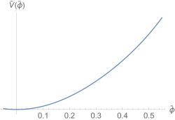
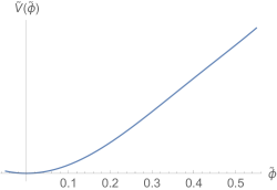
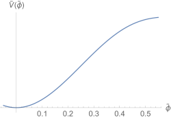
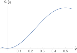
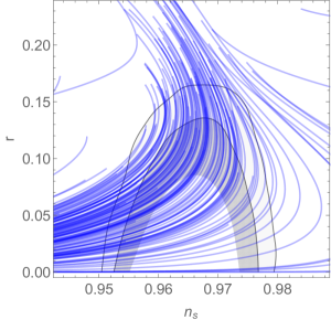
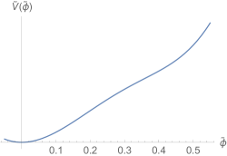
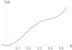
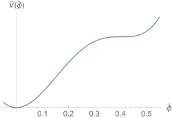
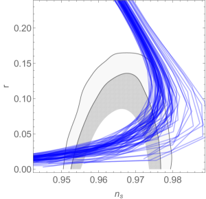
A typical example of a potential that learns to inflate is shown in Figure 1. The potential is initially drawn at random, which leads to a steep slope and correspondingly a large tensor-to-scalar ratio . As the potential learns to inflate, it flattens out, achieving a flat, approximately-linear shape. Finally, the potential starts to curve, yielding a maximum near the initial value . The large, negative second derivative near the maximum yields a negative value for the second slow-roll parameter , which in turn leads to a small value of the spectral index . Thus, we expect that the typical trajectory of a inflationary model generated by gradient ascent will begin outside the Planck 2015 exclusion limits (due to its large value of ) and end outside the exclusion limits (due to its small value of ). The question then becomes, do the trajectories pass through the inclusion regions in the intermediate regime?
A sample of 200 trajectories in the - plane is shown in figure 2. It is clear that a large fraction of the trajectories do, in fact, pass through the inclusion regions. In a study of 10,000 trajectories, we found that 64 of the trajectories passed through the inclusion region, while 34 passed through the inclusion region of the Planck 2015 data. This agreement with experiment could be interpreted as a success of our gradient ascent approach.
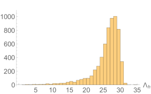
However, viewed from a quantum gravity/effective field theory perspective, these results should be viewed with caution. Figure 3 depicts the distribution of the scales for trajectories to exit the inclusion region. None of our trajectories led to a model with viable phenomenology and a sub-Planckian . Only 66 out of 10,000 trajectories remained within the inclusion region with , and only two of these 66 remained within the inclusion region with . The vast majority of the models with have and therefore disagree with experiment. This approach leads to a tension between quantum gravity and experiment.
However, if one ignores the complaints of quantum gravity and is willing to blindly consider models with super-Planckian , our gradient ascent approach predicts interesting correlations between cosmic observables. Given the observed limits on the spectral index, one expects a tensor-to-scalar ratio , which (if correct) will likely be observed within several years by forthcoming CMB experiments [64]. Assuming a sufficiently-small , our approach favors a redder tilt for the spectral index, . Our approach also predicts a field range for phenomenologically-viable inflation, .
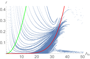
Using the fact that , we can also investigate the relationship between and the tensor-to-scalar ratio in our gradient ascent approach. While the Lyth estimate [51] gives
| (3.1) |
we find that this bound is very conservative, and indeed our hilltop trajectories are better approximated by
| (3.2) |
as shown in figure 4. One notes that some trajectories in this figure do not fit this curve at all and instead tend to give larger at smaller ! These bizarre trajectories correspond to the inflection point models of figure 5 rather than the hilltop models of figure 1. These inflection point models tend to give under this approach, so they are uninteresting from the perspective of phenomenology.
However, the strange behavior of inflection point models seen here is an artifact of this first approach, in which we fix and use this to determine . In these models, this means that almost all of the inflation is occurring along the plateau near the inflection point, but the phenomenology is being computed using the value of the slow-roll parameters at , where the first derivative of the potential is large (see figure 5 (c)-(d)). This represents a rather drastic fine-tuning of these models: has been tuned just right so that the part of the potential relevant for phenomenology represents a very tiny fraction of the total number of -foldings produced by the potential. If were decreased slightly, this potential would no longer produce enough inflation. If were increased slightly, the modes relevant for phenomenology would exit the horizon when the inflaton was rolling along the plateau, and the phenomenology would be very different. We see that while our approach of fixing and varying yields sensible results in the of trials that produced a local maximum near , it leads to issues in the of trials that produced inflection points. We therefore are lead to consider a second approach: fixing , and letting vary. We will see that this not only remedies the bizarre dependence of on , but also generates viable models of small-field inflation with .
3.2 Small-Field Inflation at Fixed , Variable
We now restrict our analysis to the “problematic” trajectories–namely, the ones that produce an inflection point rather than a local maximum. We saw that our previous approach led to problems due to an implicit fine-tuning of . To remedy this problem, we fix and allow the total number of -folds to vary, though we still compute phenomenology at a pivot scale 60 -folds before the end of inflation. As a consequence, the value at which phenomenology is determined is no longer fixed to be , but instead can vary between and (assuming that is chosen sufficiently large so that the model produces at least 60 -folds in total). Since most of the inflation occurs close to the inflection point in our models, will typically be very close to the inflection point. This alleviates the fine-tuning discussed above, which put regardless of the position of the inflection point.
How does gradient ascent act on a model with an inflection point? To good approximation, we can approximate the potential in the vicinity of an inflection point as a cubic,
| (3.3) |
Successful inflation requires . Given such a model, gradient ascent effectively decreases indefinitely without significantly altering or . Thus, given a model with set , , we can approximate the effect of gradient ascent to good accuracy by merely letting . For any fixed, no matter how small, this produces a model with arbitrarily-large number of -folds.
The phenomenology of cubic inflection models has been studied extensively [65, 66, 46], and we can make use of these results here. In particular, we may express the total number of -folds produced near an inflection point as
| (3.4) |
Then, we have
| (3.5) |
where we set . For small-field inflation, , the tensor-to-scalar ratio is too small to be detectable, so we may simply focus on the spectral index. From here, we see that our inflection point models exhibit a universal behavior in that the spectral index depends only on the total number of -folds produced by the model, and in turn the total number of -folds depends only on the ratio appearing in (3.4). Since gradient acts to simply decrease , thereby increasing , we see that will begin above the allowed range, pass through the inclusion region, and then decrease below it. In the single-field case, we see that our approach therefore makes no meaningful predictions for beyond the predictions of a generic inflection point model, since any physical information contained in , , and can be absorbed into , which depends only on the number of steps performed in the gradient ascent. Nonetheless, gradient ascent can still be a useful tool for producing such inflection point models, so it is useful to study the behavior of our model parameters from a practical perspective.
Using (3.5), we see that a phenomenologically-viable requires . Among the gradient ascent trajectories that produced an inflection point, we find that the ratio is given by
| (3.6) |
with typically and typically . Thus, for a model that produces a phenomenologically-viable , the value of is bounded below as
| (3.7) |
We see that for , must be , with decreasing drastically as decreases. This leads to practical issues with the gradient ascent. Namely, if the learning rate is too small, it can take a very long time for the inflection point to develop and to decrease to the point required for acceptable phenomenology. If the learning rate is too large, the model will overshoot the “sweet spot” with , and if it overshoots far enough, will even produce a model with , which is not monotonic on the full range . Indeed, for the learning rate used in our analysis, setting , around of the trajectories overshot the sweet spot entirely, and only of the trajectories included more than one point in the sweet spot. A better choice for the learning rate for an inflection point model would ensure that the step size is proportional to , preventing from overshooting the maximum at .
A similar statement applies to our hilltop models. In that case, the maximum of occurs not as , but rather as the position of the maximum tends towards . Overshooting the maximum , which produces an infinite number of -folds, is very common. A better choice of learning rate would ensure that the step size is proportional to . However, such small-field hilltop models are less interesting than inflection point models from the perspective of phenomenology, as they yield a value of that is too small to agree with experiment [66].
We have seen that our approaches lead to very different results depending on whether the potential develops a local maximum or an inflection point. It is therefore important to determine whether gradient ascent from some initial will produce a local maximum or an inflection point. Supervised machine learning is well-suited to this sort of task. However, in our case, we are not merely interested in making predictions but also in developing intuition. A simple logistic regression works well for this purpose:
| (3.8) |
and if gradient ascent produces a local maximum and if gradient ascent produces an inflection point. We find that this method of simple logistic regression is capable of predicting whether an initial vector of coefficients will yield an inflection point or a local maximum with an accuracy of about . The model takes the form
| (3.9) |
Of these, only and are statistically significant. When the linear combination is positive (negative), the model predicts an inflection point (local maximum). We see that the key to developing an inflection point is large, positive, initial values of . These lead to higher-order terms in the potential that continue to grow as the model learns to inflate, leading to an inflection point. On the other hand, if the higher-order terms in the potential are negative, or if the potential is dominated by lower-order terms (i.e. if are initially large), then the potential typically develops a local maximum. It is interesting that the coefficients with positive weights –namely –are precisely those that are suppressed by powers of the UV scale in effective field theory. But (especially given our distinction between the scales and ) it is unclear to us if there is any deeper reason why this should be the case.
3.3 Two-Field Inflation
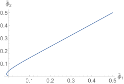
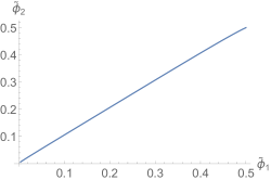
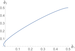
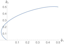
The typical evolution of the inflaton path for a two-field model that learns to inflate is shown in figure 6. An initial hierarchy in the masses of the two fields leads to a sharp bend in the inflaton path. However, the model quickly learns “isotropic -flation” [67, 68]–the hierarchy disappears, and the inflaton learns to inflate along the diagonal of two nearly-identical fields, yielding an effectively single-field model.
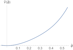
One might have expected the model to remain as a single-field model, eventually adopting a hilltop shape as we saw in the single-field case. The model does in fact develop a hilltop shape (see figure 7), but perhaps surprisingly, the dynamics of the model eventually become multi-field! As shown in figure 6 (d), the inflaton path becomes significantly curved, and grows larger than 1, violating the slow-turn approximation (see appendix C). Presumably, this is due to the fact that a curved path is longer than a straight path, so more -folds of inflation can be generated by the former than the latter. Note that if the potential were exactly symmetric in and , there would be no reason for gradient ascent to break the symmetry, so the model would remain symmetric forever. Thus, models of isotropic -flation lie along the stable direction of a hilltop-like saddle point of the function .
Shortly after the inflaton path develops significant curvature, it tends to stray too far from the origin, and the inflaton falls into a different local minimum. At this point, our gradient ascent terminates.
The phenomenology of most of the two-field models along the gradient ascent trajectory does not differ qualitatively from that of the single-field models already considered, as shown in Figure 9. Initially, the models tend to have large , but as the model learns to inflate, and both decrease. In some intermediate regime, the model falls inside the Planck inclusion region. These models do not lead to significant non-Gaussianity, and they require super-Planckian .
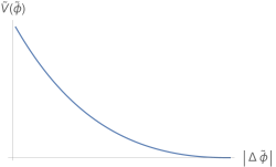
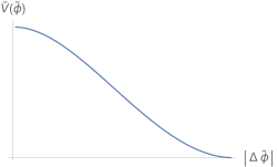
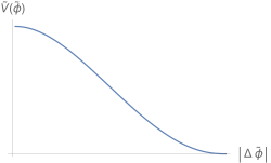
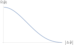
There are several differences between the single-field and two-field results, however. First, our two-field models tend to have a slightly larger , which brings them into better agreement with experiment. Indeed, over 97% of our trajectories passed through the Planck inclusion region, and 72% of trajectories passed through the inclusion region.
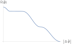
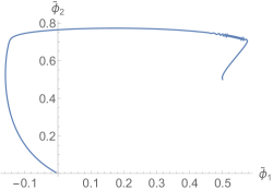
Second, our two-field models can show more complicated limiting behavior than simple local maxima or inflection points. Figure 8 shows an example of a two-field path with three plateaus (including the short one near ). This sort of behavior is quite rare, however, appearing in less that of our trials. Simple saddle points/local maxima are much more common.
Finally, as previously discussed, our two-field models eventually exhibit multi-field dynamics, as the inflaton path becomes significantly curved. This means that the slow-turn approximation we used to compute and is no longer valid, so the phenomenology of the models at the end of the trajectory will differ significantly in the two-field case vs. the single-field case.aaaNote that the slow-roll slow-turn approximation remains valid for all the models whose phenomenology is shown in figure 9, so this figure is robust. We leave an analysis of these models beyond the slow-roll slow-turn approximation for future study.
4 Comparison with GRF Inflation
How do models of inflation learned via gradient ascent compare with those generated by other means? In this section, we compare our previous results to those of Gaussian random field (GRF) models [46, 47, 48, 49]. In GRF models, the potential is taken to be a random field obeying Gaussian statistics:
| (4.1) |
with
| (4.2) |
with setting the correlation length, setting the height of the potential (which again drops out of inflationary observables , in the slow-roll approximation), and the number of fields. We will focus on single-field GRF models, so we set . Taylor expanding the potential as in (2.2),
| (4.3) |
we can translate the distribution on in (4.1) to a distribution on the coefficients . For details on how this is done, we refer the reader to [46], p. 3-7.
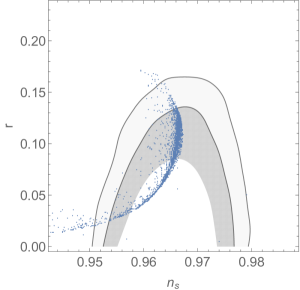
To compare with our gradient ascent models, we set and generate potentials with taking all integer values between and . For the models that produce at least 60 -folds of inflation, we compute the values of , and plot them in figure 10. We see the same qualitative features we have come to expect from random inflation models (decreasing leads to decreasing , ), though the data points from the GRF models seem to be packed closer together than we saw in gradient ascent models.
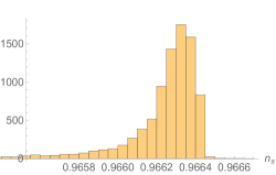
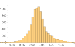
We can make this precise by analyzing the gradient ascent trajectories at a fixed scale , which we take to be . We do this as follows: for every gradient ascent trajectory, we choose the point whose value is closest to (under approach 1), restricted to those with . We similarly generate a set of GRF models with and compare the values of the gradient ascent models with those of the GRF models.
Figure 11 shows the result of this comparison. If we ignore outlying models with (at which point the second slow-roll parameter starts to grow large, and the slow-roll approximation in invalidated) the GRF approach yields a standard deviation of , whereas gradient ascent (approach 1) yields . Note also that the GRF distribution is skewed left, whereas the gradient ascent distribution is approximately symmetric.
5 Conclusions
We have examined the phenomenological predictions of a model that “learns to inflate.” Starting from random initial conditions, we computed a trajectory in the space of Wilsonian coefficients by performing a gradient ascent in the number of -folds. We found that the corresponding inflationary potentials frequently yield phenomenology in agreement with experiment.
As with all approaches to random inflation, our approach is valuable only insofar as it captures universal features of inflation. Whether or not this is the case is a very difficult question given our rudimentary knowledge of inflation and the string landscape. However, one interesting point in this regard is the similarity between large-field inflationary models generated by gradient ascent in , GRF models, and models of natural inflation [52]. Models of natural inflation are parametrized by an axion decay constant , which controls the width of the cosine and correspondingly the distance traversed by the inflaton . Natural inflation models with yield a tensor-to-scalar ratio that is too large to agree with experiment, while models with yield a spectral index that is too small. This is quite reminiscent of our results in sections 3 and 4. Indeed, parametrized as a function of , the trajectory of natural inflation in the - plane looks almost identical to one of the trajectories in figures 2 and 10, and the trajectories in figure 9 look similar but blueshifted. In this sense, one might say that our (large-field) gradient ascent models, GRF models, and natural inflation models lie in the same “universality class.” It is also worth noting that universal behavior makes individual models–such as natural inflation–harder to test; a precise measurement of , would be consistent with natural inflation, but it would also be consistent with our models produced by gradient ascent. And if gradient ascent is capable of producing said values with ease, one might suspect that other mechanisms–not just sinusoidal axion potentials produced by instantons–might also be able to produce it. Likewise, in the small-field case, our gradient ascent led to a family of inflection point models, similar to other approaches to random inflation [69].
In the two-field case, we found that gradient ascent ultimately produced a genuine multi-field model of inflation, marked by significant curvature of the inflaton path in the vast majority of cases. This differs from other approaches to random multi-field inflation, such as that of [47], which typically required fields to generate significant multi-field effects. We also saw that -flation, which involves inflating along the diagonal direction of two identical fields, represents the stable direction of a saddle point in the -folds function .
There are many possible modifications of our approach, which could be promising areas of future study. Perhaps the most obvious and pressing one is to generalize from one- and two-field inflation to -field inflation. String compactifications typically give , so it is important to understand what novel and universal behavior might arise in inflationary models in the large limit. Further, GRF and DBM models with differ significantly from those with , making it reasonable to think that large gradient ascent models will differ significantly from the ones considered here. The practical difficulty with such an analysis is that the number of terms in the inflationary potential grows exponentially with , making such studies computationally expensive. However, it is precisely in such situations, in which the number of weights (i.e. Wilsonian coefficients) grows large, that the full power of modern machine learning may prove invaluable. In particular, we used simple gradient ascent to maximize the number of -folds, but more complicated optimization methods could also be used. These methods could significantly decrease the time it takes to learn a model of inflation, especially in the many-field case.
We used a trivial kinetic term for the inflaton, but one could consider more general ones. It would be interesting to see if this approach might produce a model of DBI inflation [70] or something similar. Another possible modification is to consider an expansion in Fourier modes rather than monomials. Namely, one might consider a potential of the form
| (5.1) |
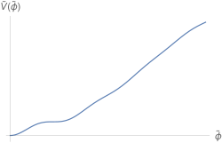
and perform a gradient ascent in the space of coefficients to maximize the number of -folds. Preliminary investigations of such models reveal that the potentials “learned” in this way typically have multiple plateaus or other jagged features, as shown in figure 12. These features could be an unwelcome indication that the model is wrong, but they might also produce interesting features in the CMB power spectrum that could be tested with experiment.
Alternative approaches to random inflation frequently encounter regions of parameter space (such as ) where significant inflation is rare, making it computationally expensive to generate enough inflationary potentials to perform a statistical analysis. In these cases, combining said approach with gradient ascent on the number of -folds could be useful for generating more inflationary potentials with -folds of inflation, reducing the computational cost.
Finally, we sought to maximize the number of -folds, but one could consider alternative reward functions. For instance, taking a bottom-up approach, one might want to condition on the observed value of the spectral index and tensor-to-scalar ratio by assigning higher value to models that agree better with experiment i.e. incorporating the Planck likelihood of the model into the reward function. From a top-down perspective, one might hope that improved understanding of the string landscape or anthropics could provide additional insight that may be incorporated into the reward function. More generally, it would interesting to see if other proposed measures for random inflation could be translated to reward functions for a model of gradient ascent.
Our approach represents just one application of machine learning techniques to theoretical cosmology. It is our hope and expectation that further applications will prove invaluable in addressing the wide array of difficult problems in cosmology and quantum gravity.
Acknowledgements
We thank Liam McAllister and Matthew Reece for comments on an earlier draft of this article, and Kyle Cranmer, Henry Lin, and Eva Silverstein for helpful discussions. The author is supported by the Carl P. Feinberg Founders Circle Membership and by NSF grant PHY-1606531.
Appendix A Gradient Ascent
The quintessential problem in machine learning is to minimize (maximize) a cost (reward) function, which is a map from a set of inputs or events into the real numbers. For instance, in a neural network, a single neuron consists of a map from some linear combination of inputs to some real number :
| (A.1) |
Here, the coefficients are called weights. In a simple neural network consisting of this single neuron, the output may be compared against some observed value , and the “cost function” may be defined as the square of the difference between the predicted and observed values, summed over all pairs of data :
| (A.2) |
The cost function effectively measures the predictive power of the model. For a particular set of inputs and output , the cost function is a function of the weights . Training the neural network amounts to determining the weights that minimize the cost function.
In practice, this minimization procedure is typically carried out through the process of gradient descent or some related method. To begin, the weights are initialized to random values . After this, subsequent values of the cost function are determined recursively according to the formula,
| (A.3) |
Here, is a parameter known as the “learning rate,” which controls how drastically the parameters of the model are allowed to change at each step. The gradient is estimated by summing over all data points as in (A.2).bbbAlternatively, in stochastic gradient descent, the gradient is estimated by summing over a random sample of data points. Stochastic gradient descent is much more efficient that ordinary gradient descent for large datasets.
In the case of a reward function , the goal is instead to maximize with respect to the weights. In this case, we use a gradient ascent rather than a gradient descent,
| (A.4) |
For an introduction to machine learning aimed at physicists, the reader may wish to consult reference [71].
Appendix B Single-Field Slow Roll Inflation
(This Slope Is Treacherous)
Cosmological inflation [72, 73, 74] is a proposed paradigm of the early universe in which quasi-exponential expansion is driven by the potential energy of one or more scalar fields. Concentrating on the case of a single scalar field, or “inflaton,” the dynamics are governed by the field equations
| (B.1) | ||||
| (B.2) |
Here, is the potential of the field , measures the rate of expansion of the universe, and we have set the reduced Planck mass equal to 1. Successful inflation requires to vary slowly with time, which implies that is approximately constant, so can be neglected. As a result the first term in (B.1) disappears, and the dynamics of effectively become a simple gradient descent towards a minimum of the potential:
| (B.3) |
To quantify the validity of the “slow-roll” approximation used above, we can define “slow-roll parameters”:
| (B.4) |
Successful slow-roll inflation requires the slow-roll parameters to be much smaller than 1. When this holds, we can translate these slow-roll conditions to conditions on the potential, defining
| (B.5) |
When these slow-roll parameters are small, they can be related by
| (B.6) |
Inflation ends when . The number of -folds of inflation, defined by , is given approximately by
| (B.7) |
Agreement with observation requires at least 50-60 -folds of inflation. Measurable quantities like the tensor-to-scalar ratio , the spectral index , and the running of the spectral index can be related to the slow-roll parameters via
| (B.8) |
Here, the ∗s indicate the values of the quantities 50-60 -folds before the end of inflation. In this paper, we take the upper limit of 60 -folds for the sake of concreteness.
More information on single-field slow-roll inflation can be found in [75].
Appendix C Two-Field Slow-Roll Inflation
(This Path is Reckless)
Two-field dynamics with a trivial field space metric are governed by the equations of motion
| (C.1) | ||||
| (C.2) |
with the two-field potential. In single-field inflation, we focused on the slow-roll regime, in which the inflaton rolls slowly down to the minimum of its potential. In two-field inflation, we work in the slow-roll, slow-turn regime, in which the inflaton rolls slowly and also turns slowly. In this approximation, we can neglect the acceleration term and approximate the dynamics with
| (C.3) |
Once again, the dynamics are effectively a gradient descent. We can again define slow-roll parameters. The first slow-roll parameter generalizes simply,
| (C.4) |
However, the second slow-roll parameter becomes a two-component vector in the two-field case. Following [62], we define
| (C.5) |
As in the single-field case, we can relate these to the shape of the potential. We define
| (C.6) |
Here and henceforth, we drop the subscript V on the slow-roll parameters defined in terms of the potential. We also define
| (C.7) |
At first order in the slow-roll slow-turn approximation, we then have
| (C.8) |
We then define the field speed , the unit vector in the direction of the gradient , and a perpendicular unit vector . At first order, we can then write
| (C.9) | ||||
| (C.10) |
then measures the speed-up rate, while measures the turn rate.
As in the single-field case, we want to relate the inflationary potential to observable quantities. For this, we need to define a unit vector in the direction of the gradient of the number of -folds, . We then define by
| (C.11) |
Then, at first order in slow-roll slow-turn, we can relate the slow-roll parameters to the tensor-to-scalar ratio and the spectral index byccc here is the spectral index for the entropic power spectrum. In this paper, we ignore the power spectrum of isocurvature modes, as they are negligible in the models we consider. Generically, multi-field models of inflation can produce a significant spectrum of isocurvature modes, and these can mix with entropic modes. [62]
| (C.12) | ||||
| (C.13) |
Note that these quantities implicitly depend on the entire trajectory of the inflaton through the function and cannot be determined simply through a local analysis of the potential.
We can also write an expression for the parameter , which measures the non-Gaussianity of the scalar power spectrum [76]:
| (C.14) |
References
- [1] L. Lucie-Smith, H. V. Peiris, A. Pontzen, and M. Lochner, “Machine learning cosmological structure formation,” arXiv:1802.04271 [astro-ph.CO].
- [2] D. Wang and W. Zhang, “Machine Learning Cosmic Expansion History,” arXiv:1712.09208 [astro-ph.CO].
- [3] H. M. Kamdar, M. J. Turk, and R. J. Brunner, “Machine learning and cosmological simulations II. Hydrodynamical simulations,” Mon. Not. Roy. Astron. Soc. 457 no. 2, (2016) 1162–1179, arXiv:1510.07659 [astro-ph.GA].
- [4] H. M. Kamdar, M. J. Turk, and R. J. Brunner, “Machine learning and cosmological simulations I. Semi-analytical models,” Mon. Not. Roy. Astron. Soc. 455 no. 1, (2016) 642–658, arXiv:1510.06402 [astro-ph.GA].
- [5] S. Ravanbakhsh, J. Oliva, S. Fromenteau, L. C. Price, S. Ho, J. Schneider, and B. Poczos, “Estimating Cosmological Parameters from the Dark Matter Distribution,” arXiv:1711.02033 [astro-ph.CO].
- [6] J. Schmelzle, A. Lucchi, T. Kacprzak, A. Amara, R. Sgier, A. Rfrgier, and T. Hofmann, “Cosmological model discrimination with Deep Learning,” arXiv:1707.05167 [astro-ph.CO].
- [7] J. Liu, “Artificial Neural Network in Cosmic Landscape,” JHEP 12 (2017) 149, arXiv:1707.02800 [hep-th].
- [8] A. Cole and G. Shiu, “Persistent Homology and Non-Gaussianity,” JCAP 1803 no. 03, (2018) 025, arXiv:1712.08159 [astro-ph.CO].
- [9] L. M. Dery, B. Nachman, F. Rubbo, and A. Schwartzman, “Weakly Supervised Classification in High Energy Physics,” JHEP 05 (2017) 145, arXiv:1702.00414 [hep-ph].
- [10] P. T. Komiske, E. M. Metodiev, B. Nachman, and M. D. Schwartz, “Pileup Mitigation with Machine Learning (PUMML),” JHEP 12 (2017) 051, arXiv:1707.08600 [hep-ph].
- [11] J. Carifio, J. Halverson, D. Krioukov, and B. D. Nelson, “Machine Learning in the String Landscape,” JHEP 09 (2017) 157, arXiv:1707.00655 [hep-th].
- [12] P. T. Komiske, E. M. Metodiev, B. Nachman, and M. D. Schwartz, “Learning to Classify from Impure Samples,” arXiv:1801.10158 [hep-ph].
- [13] L. de Oliveira, M. Paganini, and B. Nachman, “Learning Particle Physics by Example: Location-Aware Generative Adversarial Networks for Physics Synthesis,” Comput. Softw. Big Sci. 1 no. 1, (2017) 4, arXiv:1701.05927 [stat.ML].
- [14] A. Andreassen, I. Feige, C. Frye, and M. D. Schwartz, “JUNIPR: a Framework for Unsupervised Machine Learning in Particle Physics,” arXiv:1804.09720 [hep-ph].
- [15] L. de Oliveira, M. Kagan, L. Mackey, B. Nachman, and A. Schwartzman, “Jet-images deep learning edition,” JHEP 07 (2016) 069, arXiv:1511.05190 [hep-ph].
- [16] A. J. Larkoski, I. Moult, and B. Nachman, “Jet Substructure at the Large Hadron Collider: A Review of Recent Advances in Theory and Machine Learning,” arXiv:1709.04464 [hep-ph].
- [17] K. Fraser and M. D. Schwartz, “Jet Charge and Machine Learning,” arXiv:1803.08066 [hep-ph].
- [18] Y.-H. He, “Deep-Learning the Landscape,” arXiv:1706.02714 [hep-th].
- [19] P. T. Komiske, E. M. Metodiev, and M. D. Schwartz, “Deep learning in color: towards automated quark/gluon jet discrimination,” JHEP 01 (2017) 110, arXiv:1612.01551 [hep-ph].
- [20] J. H. Collins, K. Howe, and B. Nachman, “CWoLa Hunting: Extending the Bump Hunt with Machine Learning,” arXiv:1805.02664 [hep-ph].
- [21] E. M. Metodiev, B. Nachman, and J. Thaler, “Classification without labels: Learning from mixed samples in high energy physics,” JHEP 10 (2017) 174, arXiv:1708.02949 [hep-ph].
- [22] D. Krefl and R.-K. Seong, “Machine Learning of Calabi-Yau Volumes,” Phys. Rev. D96 no. 6, (2017) 066014, arXiv:1706.03346 [hep-th].
- [23] J. A. Aguilar-Saavedra, J. H. Collins, and R. K. Mishra, “A generic anti-QCD jet tagger,” JHEP 11 (2017) 163, arXiv:1709.01087 [hep-ph].
- [24] F. Ruehle, “Evolving neural networks with genetic algorithms to study the String Landscape,” JHEP 08 (2017) 038, arXiv:1706.07024 [hep-th].
- [25] A. Cole and G. Shiu, “Topological Data Analysis for the String Landscape,” arXiv:1812.06960 [hep-th].
- [26] K. Bull, Y.-H. He, V. Jejjala, and C. Mishra, “Machine Learning CICY Threefolds,” arXiv:1806.03121 [hep-th].
- [27] Y.-N. Wang and Z. Zhang, “Learning non-Higgsable gauge groups in 4D F-theory,” arXiv:1804.07296 [hep-th].
- [28] K. Hashimoto, S. Sugishita, A. Tanaka, and A. Tomiya, “Deep Learning and AdS/CFT,” arXiv:1802.08313 [hep-th].
- [29] W. J. Cunningham, High Performance Algorithms for Quantum Gravity and Cosmology. PhD thesis, Northeastern U., 2018. arXiv:1805.04463 [gr-qc].
- [30] H. Erbin and S. Krippendorf, “GANs for generating EFT models,” arXiv:1809.02612 [cs.LG].
- [31] M. Dias, J. Frazer, and A. Westphal, “Inflation as an Information Bottleneck - A strategy for identifying universality classes and making robust predictions,” arXiv:1810.05199 [hep-th].
- [32] G. Louppe, M. Kagan, and K. Cranmer, “Learning to Pivot with Adversarial Networks,” arXiv:1611.01046 [stat.ME].
- [33] T. Cohen, M. Freytsis, and B. Ostdiek, “(Machine) Learning to Do More with Less,” JHEP 02 (2018) 034, arXiv:1706.09451 [hep-ph].
- [34] K. Datta and A. J. Larkoski, “Novel Jet Observables from Machine Learning,” JHEP 03 (2018) 086, arXiv:1710.01305 [hep-ph].
- [35] J. Brehmer, K. Cranmer, G. Louppe, and J. Pavez, “Constraining Effective Field Theories with Machine Learning,” Phys. Rev. Lett. 121 no. 11, (2018) 111801, arXiv:1805.00013 [hep-ph].
- [36] T. Heimel, G. Kasieczka, T. Plehn, and J. M. Thompson, “QCD or What?,” arXiv:1808.08979 [hep-ph].
- [37] M. Farina, Y. Nakai, and D. Shih, “Searching for New Physics with Deep Autoencoders,” arXiv:1808.08992 [hep-ph].
- [38] M. Tegmark, “What does inflation really predict?,” JCAP 0504 (2005) 001, arXiv:astro-ph/0410281 [astro-ph].
- [39] J. Frazer and A. R. Liddle, “Exploring a string-like landscape,” JCAP 1102 (2011) 026, arXiv:1101.1619 [astro-ph.CO].
- [40] M. C. D. Marsh, L. McAllister, E. Pajer, and T. Wrase, “Charting an Inflationary Landscape with Random Matrix Theory,” JCAP 1311 (2013) 040, arXiv:1307.3559 [hep-th].
- [41] F. G. Pedro and A. Westphal, “Inflation with a graceful exit in a random landscape,” JHEP 03 (2017) 163, arXiv:1611.07059 [hep-th].
- [42] G. Wang and T. Battefeld, “Random Functions via Dyson Brownian Motion: Progress and Problems,” JCAP 1609 no. 09, (2016) 008, arXiv:1607.02514 [hep-th].
- [43] B. Freivogel, R. Gobbetti, E. Pajer, and I.-S. Yang, “Inflation on a Slippery Slope,” arXiv:1608.00041 [hep-th].
- [44] M. Dias, J. Frazer, and M. c. D. Marsh, “Seven Lessons from Manyfield Inflation in Random Potentials,” JCAP 1801 no. 01, (2018) 036, arXiv:1706.03774 [astro-ph.CO].
- [45] S. Paban and R. Rosati, “Inflation in Multi-field Modified DBM Potentials,” JCAP 1809 no. 09, (2018) 042, arXiv:1807.07654 [astro-ph.CO].
- [46] A. Masoumi, A. Vilenkin, and M. Yamada, “Inflation in random Gaussian landscapes,” JCAP 1705 no. 05, (2017) 053, arXiv:1612.03960 [hep-th].
- [47] T. Bjorkmo and M. C. D. Marsh, “Manyfield Inflation in Random Potentials,” JCAP 1802 no. 02, (2018) 037, arXiv:1709.10076 [astro-ph.CO].
- [48] T. C. Bachlechner, “On Gaussian Random Supergravity,” JHEP 04 (2014) 054, arXiv:1401.6187 [hep-th].
- [49] R. Easther, A. H. Guth, and A. Masoumi, “Counting Vacua in Random Landscapes,” arXiv:1612.05224 [hep-th].
- [50] A. Masoumi, A. Vilenkin, and M. Yamada, “Initial conditions for slow-roll inflation in a random Gaussian landscape,” JCAP 1707 no. 07, (2017) 003, arXiv:1704.06994 [hep-th].
- [51] D. H. Lyth, “What would we learn by detecting a gravitational wave signal in the cosmic microwave background anisotropy?,” Phys.Rev.Lett. 78 (1997) 1861–1863, arXiv:hep-ph/9606387 [hep-ph].
- [52] K. Freese, J. A. Frieman, and A. V. Olinto, “Natural inflation with pseudo - Nambu-Goldstone bosons,” Phys.Rev.Lett. 65 (1990) 3233–3236.
- [53] T. Banks, M. Dine, P. J. Fox, and E. Gorbatov, “On the possibility of large axion decay constants,” JCAP 0306 (2003) 001, arXiv:hep-th/0303252 [hep-th].
- [54] T. Rudelius, “On the Possibility of Large Axion Moduli Spaces,” JCAP 1504 no. 04, (2015) 049, arXiv:1409.5793 [hep-th].
- [55] C. Long, L. McAllister, and J. Stout, “Systematics of Axion Inflation in Calabi-Yau Hypersurfaces,” arXiv:1603.01259 [hep-th].
- [56] J. P. Conlon and S. Krippendorf, “Axion decay constants away from the lamppost,” JHEP 04 (2016) 085, arXiv:1601.00647 [hep-th].
- [57] N. Arkani-Hamed, L. Motl, A. Nicolis, and C. Vafa, “The String landscape, black holes and gravity as the weakest force,” JHEP 0706 (2007) 060, arXiv:hep-th/0601001 [hep-th].
- [58] T. Rudelius, “Constraints on Axion Inflation from the Weak Gravity Conjecture,” JCAP 09 (2015) 020, arXiv:1503.00795 [hep-th].
- [59] M. Montero, A. M. Uranga, and I. Valenzuela, “Transplanckian axions!?,” JHEP 08 (2015) 032, arXiv:1503.03886 [hep-th].
- [60] J. Brown, W. Cottrell, G. Shiu, and P. Soler, “Fencing in the Swampland: Quantum Gravity Constraints on Large Field Inflation,” arXiv:1503.04783 [hep-th].
- [61] B. Heidenreich, M. Reece, and T. Rudelius, “Weak Gravity Strongly Constrains Large-Field Axion Inflation,” arXiv:1506.03447 [hep-th].
- [62] C. M. Peterson and M. Tegmark, “Testing Two-Field Inflation,” Phys. Rev. D83 (2011) 023522, arXiv:1005.4056 [astro-ph.CO].
- [63] B. Freivogel, M. Kleban, M. Rodriguez Martinez, and L. Susskind, “Observational consequences of a landscape,” JHEP 03 (2006) 039, arXiv:hep-th/0505232 [hep-th].
- [64] CMB-S4 Collaboration, K. N. Abazajian et al., “CMB-S4 Science Book, First Edition,” arXiv:1610.02743 [astro-ph.CO].
- [65] D. Baumann, A. Dymarsky, I. R. Klebanov, and L. McAllister, “Towards an Explicit Model of D-brane Inflation,” JCAP 0801 (2008) 024, arXiv:0706.0360 [hep-th].
- [66] A. D. Linde and A. Westphal, “Accidental Inflation in String Theory,” JCAP 0803 (2008) 005, arXiv:0712.1610 [hep-th].
- [67] A. R. Liddle, A. Mazumdar, and F. E. Schunck, “Assisted inflation,” Phys. Rev. D58 (1998) 061301, arXiv:astro-ph/9804177 [astro-ph].
- [68] S. Dimopoulos, S. Kachru, J. McGreevy, and J. G. Wacker, “N-flation,” JCAP 0808 (2008) 003, arXiv:hep-th/0507205 [hep-th].
- [69] L. McAllister, S. Renaux-Petel, and G. Xu, “A Statistical Approach to Multifield Inflation: Many-field Perturbations Beyond Slow Roll,” JCAP 1210 (2012) 046, arXiv:1207.0317 [astro-ph.CO].
- [70] E. Silverstein and D. Tong, “Scalar speed limits and cosmology: Acceleration from D-cceleration,” Phys. Rev. D70 (2004) 103505, arXiv:hep-th/0310221 [hep-th].
- [71] P. Mehta, M. Bukov, C.-H. Wang, A. G. R. Day, C. Richardson, C. K. Fisher, and D. J. Schwab, “A high-bias, low-variance introduction to Machine Learning for physicists,” arXiv:1803.08823 [physics.comp-ph].
- [72] A. H. Guth, “The Inflationary Universe: A Possible Solution to the Horizon and Flatness Problems,” Phys. Rev. D23 (1981) 347–356.
- [73] A. Albrecht and P. J. Steinhardt, “Cosmology for Grand Unified Theories with Radiatively Induced Symmetry Breaking,” Phys. Rev. Lett. 48 (1982) 1220–1223.
- [74] A. D. Linde, “A New Inflationary Universe Scenario: A Possible Solution of the Horizon, Flatness, Homogeneity, Isotropy and Primordial Monopole Problems,” Phys. Lett. B108 (1982) 389–393.
- [75] D. Baumann, “Inflation,” in Physics of the large and the small, TASI 09, proceedings of the Theoretical Advanced Study Institute in Elementary Particle Physics, Boulder, Colorado, USA, 1-26 June 2009, pp. 523–686. 2011. arXiv:0907.5424 [hep-th]. https://inspirehep.net/record/827549/files/arXiv:0907.5424.pdf.
- [76] C. M. Peterson and M. Tegmark, “Non-Gaussianity in Two-Field Inflation,” Phys. Rev. D84 (2011) 023520, arXiv:1011.6675 [astro-ph.CO].