Stochastic Approximation Hamiltonian Monte Carlo

Stochastic Approximation Hamiltonian Monte Carlo

Abstract

Recently, the Hamilton Monte Carlo (HMC) has become widespread as one of the more reliable approaches to efficient sample generation processes. However, HMC is difficult to sample in a multimodal posterior distribution because the HMC chain cannot cross energy barrier between modes due to the energy conservation property. In this paper, we propose a Stochastic Approximate Hamilton Monte Carlo (SAHMC) algorithm for generating samples from multimodal density under the Hamiltonian Monte Carlo (HMC) framework. SAHMC can adaptively lower the energy barrier to move the Hamiltonian trajectory more frequently and more easily between modes. Our simulation studies show that the potential for SAHMC to explore a multimodal target distribution more efficiently than HMC based implementations.

Keywords: Hamiltonian Monte Carlo; Stochastic approximation Monte Carlo; multimodality;
                       Scalable computation; Neural Networks

1 Introduction

Markov chain Monte Carlo (MCMC) is one of the conventional algorithms for Bayesian inference to generate samples from the posterior distribution. However, many proposed MCMC algorithms are very inefficient due to randomness in sample generation. Recently, HMC (Duane et al., 1987; Neal, 2010), which imitates Hamiltonian dynamics in the sample generation procedure, has gained popularity in the MCMC communities as one of the efficient sampling methods (Carpenter et al., 2017a).

To construct the MCMC using Hamiltonian dynamics, first define a Hamiltonian function for the posterior probability distribution for which you want to generate a sample. The Hamiltonian function consists of two variables: the ”position” variable corresponding to the realization from the posterior probability distribution, and the auxiliary ”momentum” variable, which helps the chain to produce efficient samples using energy conservation characteristics. Typically, an independent Gaussian distribution (Neal, 2010) or Riemannian manifold (RMHMC: Fisher information) (Girolami and Calderhead, 2011) are assumed for the momentum variable. By updating the momentum variable, a new state can be proposed by calculating the trajectories moving along the same set of levels according to the energy conservation properties. The state proposed by Hamiltonian mechanics can be far from the current state, but nonetheless it is likely to accept the sample.

HMC can be classified as one of the auxiliary variable MCMC algorithms and is called hybrid Monte Carlo because it combines MCMC and the deterministic simulation algorithm, the leapfrog method for implementing Hamiltonian dynamics. The tuning parameters of the leapfrog method, leapfrog step-size, $\epsilon$, and the number of leapfrog, $L$ are one of the practical issues in implementing the HMC. The no-U-turn sampler (NUTS) has been proposed by Hoffman and Gelman (2014) to eliminate the need to set the HMCs the number of leapfrog, by stopping trajectory automatically when it starts to double back and retrace its steps. A detailed description of HMC based on geometric foundations is given in Betancourt et al. (2014) and the theoretical properties of HMC have been studied in Livingstone et al. (2016) and Durmus et al. (2017).

One of the well-known problems in HMC is the generation of samples from multimodal posterior distributions. HMC and its variants (Girolami and Calderhead, 2011; Hoffman and Gelman, 2014; Neal, 2010; Shahbaba et al., 2013; Sohl-Dickstein et al., 2014) cannot easily move from one mode to another within a small number of iterations because the energy barrier between modes is high when the parameters of interest have different modes separated by low probability areas.

Several variants of the HMC algorithm have been proposed to solve the multimodality problem of HMC. Wormhole Hamiltonian Monte Carlo (WHMC, Lan et al. (2014)) modifies the RMHMC (Girolami and Calderhead, 2011) to create a short path (a so-called wormhole) that connects modes to facilitate movement between modes. This method is useful if detailed and accurate knowledge about modes are provided, but such requirement is not practical in high-dimensional multimodal distributions. To resolve this issue, WHMC employs a mode discovering mechanism. According to Fok et al. (2017), however, this mechanism still requires some knowledge about the target distribution; otherwise it may unstabilize WHMC.

A tempering approach is combined with HMC in Nishimura and Dunson (2016) and the authors suggest a new type of mass matrix to lower the energy barrier between modes so that the trajectory of Hamiltonian mechanics can move more often from one mode to the other. However, this algorithm must specify an appropriate temperature schedule so that the trajectory can efficiently navigate the parameter space. In addition, the standard integrator is not applicable to this sampler because the velocity of this sampler is unbounded in the area of the low probability region. Last, this algorithm uses a non-volume preserving integrator, therefore it requires to calculate the determinant of the Jacobian for the acceptance probability.

In this article, we propose a new algorithm, Stochastic Approximation Hamiltonian Monte Carlo (SAHMC), for generating samples from a multimodal density under the framework of the HMC. SAHMC is an HMC version of the Stochastic Approximation Monte Carlo (SAMC) algorithm (Liang, 2007; Liang et al., 2007), which draws samples from each subregions with a predetermined frequency. SAHMC use weights in SAMC, which are updated proportionate to the differences between actual number of visits of subregions with the prespecified frequency using stochastic approximation (Robbins and Monro, 1951), to adaptively lower the energy barrier between modes and allow chains to easily pass through low probability areas between modes. The convergence of the algorithm is established under mild conditions. Compared to Lan et al. (2014), SAHMC does not need to know the location of the mode before implementation. Compared to Nishimura and Dunson (2016), the specification of neither temperature schedule nor variable-step integrators is required for SAHMC implementations. Numerical results show that the new algorithm works well, especially if the target density is a high-dimensional multimodal distribution.

The rest of the article is organized as follows. In Section 2, we describe the SAMC algorithm. In Section 3, we incorporate HMC under the framework of SAMC and study its theoretical property. In Section 4, we test our SAHMC algorithm to the Gaussian mixture models along with extensive comparison with HMC. In Section 5, we apply our SAHMC to neural network model and compare results with HMC. In Section 6, we conclude the article with brief discussions.

2 SAMC Algorithm

Suppose that we are interested in sampling from the distribution

$$f({\bf x})=c\psi({\bf x}),\quad{\bf x}\in{\cal X},$$ (1)

where $c$ is an unknown normalizing constant and ${\cal X}$ is the sample space. For mathematical convenience, we assume that ${\cal X}$ is either finite or compact.

We let $E_{1}$, $\cdots$, $E_{m}$ denote $m$ partition of ${\cal X}$ according to the potential energy function, $U({\bf x})=-\log\psi({\bf x})$, i.e., $E_{1}=\big{\{}{\bf x}:U({\bf x})\leq u_{1},{\bf x}\in{\cal X}\big{\}}$, $E_{2}=\big{\{}{\bf x}:u_{1}<U({\bf x})\leq u_{2},{\bf x}\in{\cal X}\big{\}}$, $\cdots$, $E_{m-1}=\big{\{}{\bf x}:u_{m-2}<U({\bf x})\leq u_{m-1},{\bf x}\in{\cal X}\big{\}}$, and $E_{m}=\big{\{}{\bf x}:U({\bf x})>u_{m-1},{\bf x}\in{\cal X}\big{\}}$, where $u_{1}<u_{2}<\cdots<u_{m-1}$ are pre-specified numbers. Let $\bm{\pi}=(\pi_{1},\cdots,\pi_{m})$ be an $m$-vector with $0<\pi_{i}<1$ and $\sum_{i=1}^{m}\pi_{i}=1$, and denote the desired sampling frequency for each of the subregions. In general, $\pi$’s are chosen to be uniform when there are no prior knowledge availalbe about $\psi(\bf x)$. Then, the estimate of equation (1) can be written as

$$f_{\omega}(x)\propto\sum_{i=1}^{m}\frac{\pi_{i}\psi({\bf x})}{\omega_{i}}I\big{(}{\bf x}\in E_{i}\big{)}.$$ (2)

where the partition of normalizing constant, $\omega_{i}=\int_{E_{i}}\psi({\bf x})dx$. SAMC allows the existence of empty subregions in simulations and provides an automatic way to learn the normalizing constants $\omega_{1}$, $\cdots$, $\omega_{m}$.

Let $\{a_{t}\}$ denote the gain factor sequence which is positive, non-increasing sequence satisfying

$$\mbox{(a)}\quad\sum_{t=1}^{\infty}a_{t}=\infty,\qquad\mbox{and}\qquad\mbox{(b)}\quad\sum_{t=1}^{\infty}a_{t}^{\zeta}<\infty.$$ (3)

for some $\zeta\in(1,2)$. For example, (Liang et al., 2007) suggests

$$a_{t}=\frac{t_{0}}{\max(t_{0},t)},\qquad t=1,2,\cdots$$ (4)

for some specified value of $t_{0}>1$.

Let $\theta_{i}^{(t)}$ denote a working estimate of $\log(\omega_{i}/\pi_{i})$ obtained at iteration $t$, and let $\bm{\theta}^{(t)}=(\theta_{1}^{(t)},\ldots,\theta_{m}^{(t)})$. With the foregoing notation, one iteration of SAMC can be described as follows:

SAMC Algorithm

1. (Sample Generation) Simulate a sample ${\bf x}^{(t+1)}$ by a single MH update, of which the invariant distribution is a working estimate of $f_{\omega}(x)$ at iteration $t$.

2. ($\theta$-updating step) Set

   $$\bm{\theta}^{*}=\bm{\theta}^{(t)}+a_{t+1}\Big{(}{\bf e}_{t}-\bm{\pi}\Big{)},$$

   where ${\bf e}_{t}=\big{(}e_{t,1},\cdots,e_{t,m}\big{)}$ and $e_{t,i}=1$ if ${\bf x}_{t}\in E_{i}$ and 0 otherwise. If $\bm{\theta}^{*}\in\Theta$, set $\bm{\theta}^{(t+1)}=\bm{\theta}^{*}$; otherwise, set $\bm{\theta}^{(t+1)}=\bm{\theta}^{*}+{\bf c}^{*}$, where ${\bf c}^{*}=\big{(}c^{*},\cdots,c^{*}\big{)}$ can be an arbitrary vector which satisfies the condition $\bm{\theta}^{*}+{\bf c}^{*}\in\Theta$.

For effective implementation of SAMC, several issues must be considered (Liang et al., 2007):

• Sample Space Partition  The sample space are partitioned according to our goal and the complexity of the given problem. For example, when we generate samples from the distribution, the sample space can be partitioned according to the energy function. The maximum energy difference in each subregion should be bounded, for example, Liang et al. (2007) suggests to use 2. Within the same subregion, the behavior of the SAHMC move reduces to the local HMC.

• Choice of the desired sampling distribution  If we aim to estimate $\bm{\omega}$, then we may set the desired distribution to be uniform, as is done in all examples in this article. However, we may set the desired distribution biased to low-energy regions. To ensure convergence, the partition of all sample spaces must be visited in proportion to the desired sampling distribution.

• Choice of $t_{0}$ and the number of iterations  To estimate $\bm{\omega}$, $\alpha_{t}$ should be very close to 0 at the end of simulations and the speed of $\alpha_{t}$ going to 0 can be controlled by $t_{0}$. In practice, we choose $t_{0}$ according to the complexity of the problem; The more complex the problem is, the larger the value of $t_{0}$ that should be chosen. A large $t_{0}$ will make SAHMC reach all subregions quickly, even in the presence of multiple local energy minima.

3 SAHMC Algorithm

To substitute the sample generation step in SAMC to HMC, we at first define the potential energy function as

$$U({\bf x})=-\log\psi({\bf x})$$ (5)

and the kinetic energy function as

$$K({\bf y})=\frac{d}{2}\log(2\pi)+\frac{1}{2}\log|{\bf M}|+\frac{1}{2}{\bf y}{\bf M}^{-1}{\bf y},$$ (6)

where the auxiliary variable ${\bf y}$ is interpreted as a momentum variable, $d$ is the dimension of ${\bf x}$, and covariance matrix ${\bf M}$ denotes a mass matrix. We can prespecify the mass matrix $M$ using a diagonal matrix or define it using the Riemannian manifold (Girolami and Calderhead, 2011)… Then, the Hamiltonian and its corresponding probability function are

$$H({\bf x},{\bf y})=U({\bf x})+K({\bf y})\qquad\mbox{and}\qquad g({\bf x},{\bf y})\propto\exp\Big{\{}-U\big{(}{\bf x}\big{)}-K\big{(}{\bf y}\big{)}\Big{\}}$$ (7)

The partial derivatives of $H({\bf x},{\bf y})$ determines how ${\bf x}$ and ${\bf y}$ change over time, according to Hamiltonian equation,

$$\begin{split}\dot{{\bf x}}&=~{}~{}~{}\bigtriangledown_{{\bf y}}H({\bf x},{\bf y})=~{}~{}~{}{\bf M}^{-1}{\bf y}\\ \dot{{\bf y}}&=-\bigtriangledown_{{\bf x}}H({\bf x},{\bf y})=-\bigtriangledown_{{\bf x}}U({\bf x})\end{split}$$ (8)

Note that ${\bf M}^{-1}{\bf y}$ can be interpreted as velocity.

Under the aforementioned energy partition, the estimate of equation (1) can be written as

$$f_{\omega}(x)\propto\sum_{i=1}^{m}\frac{\pi_{i}\psi({\bf x})}{\omega_{i}}I\big{(}{\bf x}\in E_{i}\big{)}=\sum_{i=1}^{m}\int_{\cal Y}\frac{\pi_{i}g({\bf x},{\bf y})}{\omega_{i}}I\big{(}{\bf x}\in E_{i}\big{)}dy.$$ (9)

where the partition of normalizing constant, $\omega_{i}$, is

$$\omega_{i}=\int_{E_{i}}\psi({\bf x})dx=\int_{E_{i}}\int_{\cal Y}g({\bf x},{\bf y})dydx.$$ (10)

SAHMC allows the existence of empty subregions in simulations and provides an automatic way to learn the normalizing constants $\omega_{1}$, $\cdots$, $\omega_{m}$.

Let $\theta_{t}^{i}$ denote a working estimate of $\log(\omega_{i}^{t}/\pi_{i})$ obtained at iteration $t$ where $\omega_{i}^{t}$ is the $\omega_{i}$ value at iteration $t$, and

$$f_{\theta_{t}^{i}}(x)\propto\frac{\psi({\bf x})}{\exp(\theta_{t}^{i})}I\big{(}{\bf x}\in E_{i}\big{)}=\int_{\cal Y}\frac{g({\bf x},{\bf y})}{\exp(\theta_{t}^{i})}I\big{(}{\bf x}\in E_{i}\big{)}dy.$$

With the foregoing notation, one iteration of SAHMC can be described as follows:

SAHMC Algorithm

1. (Momentum Updating) Draw an independent normal random variable ${\bf y}\sim N_{d}\big{(}0,{\bf M}\big{)}$, and set ${\bf y}_{t}={\bf y}$ and $K_{t}=K\big{(}{\bf y}_{t}\big{)}$. Also, set ${\bf x}_{t}={\bf x}$ and $U_{t}=U\big{(}{\bf x}_{t}\big{)}$.

2. (Proposal Step)

   1. Set ${\bf x}_{t}^{0}={\bf x}_{t}$. Make a half step for the momentum at the beginning with

      $${\bf y}_{t}^{0}\leftarrow{\bf y}_{t}-\frac{\epsilon}{2}\times\frac{\partial U({\bf x}_{t})}{\partial{\bf x}}\bigg{]}_{{\bf x}_{t}^{0}}.$$

   2. Alternate full steps for position and momentum. For $i=1,\cdots,L-1$, do the following

      1. Make a full step for the position: ${\bf x}_{t}^{i}\leftarrow{\bf x}_{t}^{i-1}+\epsilon\times{\bf y}_{t}^{i-1}$.

      2. Make a full step for the momentum, except at the end of trajectory:

         $${\bf y}_{t}^{i}\leftarrow{\bf y}_{t}^{i-1}-\epsilon\times\frac{\partial U({\bf x}_{t}^{i})}{\partial{\bf x}}\bigg{]}_{x_{t}^{i}}.$$

   3. Make a half step for momentum at the end:

      $${\bf y}_{t}^{L}\leftarrow{\bf y}_{t}^{L-1}-\frac{\epsilon}{2}\times\frac{\partial U({\bf x}_{t}^{L})}{\partial{\bf x}}\bigg{]}_{{\bf x}_{t}^{L}}.$$

   4. Set negative momentum at the end of trajectory to make the proposal symmetric: ${\bf y}_{*}=-{\bf y}_{t}^{L}$. Also, set ${\bf x}_{*}={\bf x}_{t}^{L}$.

3. (Decision Step) Set $U_{*}=U({\bf x}_{*})$ and $K_{*}=K({\bf y}_{*})$, calculate

   $$r=\exp\Big{\{}\theta_{t}^{J(U_{t})}-\theta_{t}^{J(U_{*})}\Big{\}}\exp\Big{\{}U_{t}+K_{t}-U_{*}-K_{*}\Big{\}},$$ (11)

   where $J(U_{t})$ denotes the index of the subregion that ${\bf x}_{t}$ belongs to. Accept the proposal with probability $\min(1,r)$. If accepted, set ${\bf x}_{t+1}={\bf x}_{*}$; otherwise ${\bf x}_{t+1}={\bf x}_{t}$.

4. ($\theta$-updating step) Set

   $$\bm{\theta}_{*}=\bm{\theta}_{t}+a_{t+1}\Big{(}{\bf e}_{t}-\bm{\pi}\Big{)},$$

   where ${\bf e}_{t}=\big{(}e_{t,1},\cdots,e_{t,m}\big{)}$ and $e_{t,i}=1$ if ${\bf x}_{t}\in E_{i}$ and 0 otherwise. If $\bm{\theta}_{*}\in\Theta$, set $\bm{\theta}_{(t+1)}=\bm{\theta}_{*}$; otherwise, set $\bm{\theta}_{(t+1)}=\bm{\theta}_{*}+{\bf c}^{*}$, where ${\bf c}^{*}=\big{(}c^{*},\cdots,c^{*}\big{)}$ can be an arbitrary vector which satisfies the condition $\bm{\theta}_{*}+{\bf c}^{*}\in\Theta$.

In general, $\Theta$ is chosen to be a large compact set (e.g. $[-10^{100},10^{100}]^{m}$), which is practically equivalent to $\mathbb{R}^{m}$. Thanks to the location invariance of the target distribution, a choice of a constant vector $\bf{c}^{*}$ does not affect the theoretical convergence of SAHMC algorithm.

Like SAMC (Liang, 2009; Liang et al., 2007), SAHMC also falls into the category of stochastic approximation algorithms (Andrieu et al., 2005; Benveniste et al., 1990), and the theoretical convergence results are provided in the Appendix. The theory states that under mind conditions, we have

$$\theta_{t}^{i}\to\left\{\begin{array}[]{lc}C+\log\bigg{(}\int_{E_{i}}\int_{\cal Y}g\big{(}{\bf x},{\bf y}\big{)}dydx\bigg{)}-\log\Big{(}\pi_{i}+\nu\Big{)},&\mbox{if}~{}E_{i}\neq\phi\\ -\infty&\mbox{if}~{}E_{i}=\phi\end{array}\right.$$ (12)

where $\nu=\sum_{j\in\{i:E_{i}=\phi\}}\pi_{j}/(m-m_{0})$ and $m_{0}$ is the number of empty subregions, and $C$ represents an arbitrary constant. Since $f_{\bm{\theta}_{t}}({\bf x})=\sum\nolimits_{i=1}^{m}f_{\theta_{t}^{i}}(\bf x)$ is invariant with respect to a location transformation of $\bm{\theta}_{t}$, $C$ cannot be determined by the SAHMC samples. To determine the value of $C$, extra information is needed; for example, $\sum_{i=1}^{m}e^{\theta_{t}^{i}}$ is equal to a known number.

The main advantage of the SAHMC algorithm is that it can adaptively lower the energy barrier between modes and move the Hamiltonian trajectory more frequently and easily across the low probability regions between modes. In the meanwhile, the HMC trajectory cannot move to another mode beyond the energy barrier (Nishimura and Dunson, 2016).

The energy barrier with respect to $U({\bf x})$ from a position ${\bf x}_{1}$ to ${\bf x}_{2}$, is the minimum amount of kinetic energy $K({\bf x})$ to reach ${\bf x}_{2}$ from ${\bf x}_{1}$ in a single iteration (Nishimura and Dunson, 2016):

$$B_{H}\Big{(}{\bf x}_{1},{\bf x}_{2};U\Big{)}=\inf_{\bm{\gamma}\in C^{0}}\bigg{\{}\max_{0\leq t\leq 1}U\big{(}\bm{\gamma}(t)\big{)}-U\big{(}{\bf x}_{1}\big{)}\mid\bm{\gamma}\big{(}0\big{)}={\bf x}_{1}~{}\mbox{and}~{}\bm{\gamma}\big{(}1\big{)}={\bf x}_{2}\bigg{\}}$$ (13)

where $C^{0}$ denotes a class of continuous function. Note that due to the energy conservation property,

$$U\big{(}{\bf x}_{t}\big{)}-U\big{(}{\bf x}_{1}\big{)}=K\big{(}{\bf x}_{1}\big{)}-K\big{(}{\bf x}_{t}\big{)}\leq K\big{(}{\bf x}_{1}\big{)}.$$ (14)

If the kinetic energy of $K\big{(}{\bf x}_{1}\big{)}$ is less than the energy barrier $B\big{(}{\bf x}_{1},{\bf x}_{2};U\big{)}$, then HMC will not be able to reach ${\bf x}_{2}$. However, for SAHMC, the equation (13) can be rewritten as

$$B_{SA}\Big{(}{\bf x}_{1},{\bf x}_{2};U\Big{)}=\inf_{\bm{\gamma}\in C^{0}}\bigg{\{}\max_{0\leq t\leq 1}U\big{(}\bm{\gamma}(t)\big{)}-U\big{(}{\bf x}_{1}\big{)}+\Big{(}\theta^{J(U_{t})}-\theta^{J(U_{1})}\Big{)}\bigg{|}\bm{\gamma}\big{(}0\big{)}={\bf x}_{1}~{}\mbox{and}~{}\bm{\gamma}\big{(}1\big{)}={\bf x}_{2}\bigg{\}}$$ (15)

where $J(U_{t})$ and $J(U_{1})$ denote the index of the subregions that ${\bf x}_{\bm{\gamma}(t)}$ and ${\bf x}_{1}$ belong to, respectively. From our assumption that the chain currently stays near ${\bf x}_{1}$ for several iterations. That means the sample of $J(U_{1})$ is oversampled than $\pi_{J(U_{1})}$, while the sample of $J(U_{t})$ is undersampled than $\pi_{J(U_{t})}$, resulting in $\theta^{J(U_{1})}$ being larger than $\theta^{J(U_{t})}$. Then, under the SAHMC framework, the energy barrier can be lowered by $\theta^{J(U_{t})}-\theta^{J(U_{1})}$, so kinetic energy in $K\big{(}{\bf x}_{1}\big{)}$ can move the trajectory more easily than in other modes ${\bf x}_{2}$. The amount of energy barriers lowered by SAHMC is determined adaptively according to the frequency of visits to the subregion.

The other benefit of the SAHMC algorithm is its flexibility for other variants of the HMC. Because SAHMC can be implemented by adding one more step to the HMC, all existing HMC variants can be easily implemented under the SAHMC framework. For example, by replacing mass matrix ${\bf M}$ with Fisher information matrix, we can easily implement RMHMC (Girolami and Calderhead, 2011) under the framework of SAHMC.

4 Illustrative Examples

4.1 Gaussian Mixture Distributions

Table 1: Gaussian Mixture Examples: Comparison of SAHMC, HMC and NUTS

Set 1: a = -6, b = 4
Parameter	Method	Time(s)	ESS (min, med, max)	s / min ESS	Relative Speed
$x_{1}$	HMC	30.6	( 787, 882, 941)	0.03888	1.00
	SAHMC	30.6	(2041, 2984, 3549)	0.01499	2.59
	NUTS	30.0	(32, 50, 225)	0.93750	0.04
$x_{2}$	HMC	30.6	( 802, 879, 950)	0.03815	1.00
	SAHMC	30.6	(2120, 3034, 3493)	0.01443	2.64
	NUTS	30.0	(31, 50, 236)	0.96774	0.04
Set 2: a = -8, b = 6
Parameter	Method	Time(s)	ESS (min, med, max)	s / min ESS	Relative Speed
$x_{1}$	HMC	30.6	( 18, 25, 78)	1.70000	1.00
	SAHMC	30.6	(533, 723, 1033)	0.05741	29.61
	NUTS	19.0	(3, 3060, 9700)	6.33333	0.27
$x_{2}$	HMC	30.6	( 17, 26, 78)	1.80000	1.00
	SAHMC	30.6	(581, 683, 825)	0.05267	34.18
	NUTS	19.0	(3, 3479, 8841)	6.33333	0.28

As our illustrative example, we compare SAHMC with HMC and NUTS using the following Gaussian mixture distribution:

$$p({\bf x})=\frac{1}{3}N_{2}\left[\left(\begin{array}[]{c}a\\ a\end{array}\right),\left(\begin{array}[]{cc}1&0.9\\ 0.9&1\end{array}\right)\right]+\frac{1}{3}N_{2}\left[\left(\begin{array}[]{c}b\\ b\end{array}\right),\left(\begin{array}[]{cc}1&-0.9\\ -0.9&1\end{array}\right)\right]+\frac{1}{3}N_{2}\Big{[}{\bf 0},I_{2}\Big{]}$$ (16)

which is identical to that given by Gilks et al. (1998) except that the mean vectors are separated by a larger distance in each dimension. With this example, we show how SAHMC outperform to the original HMC method in generating samples from multimodal density.

NUTS improves upon HMC by automatically choosing optimal values for HMC’s tunable method parameters. It has been shown that NUTS samples complex distributions effectively (Henderson and Goggans, 2019). NUTS can be easily implemented using Stan software Carpenter et al. (2017b) , which is available in many popular computing environments including R, Python, Julia, MATLAB, etc.

We used two sets of $(a,b)$; $(-6,4)$ and $(-8,6)$. For both HMC and SAHMC, we set the leapfrog step-size, $\epsilon=0.3$, and leapfrog steps, $L=20$. We used the identity mass matrices of HMC and SAHMC, so for fair comparison we used the identity mass matrix for NUTS. For NUTS implementation, the stepsize, $\epsilon$ is tuned using the dual-averaging algorithm of Hoffman and Gelman (2014) so that the average acceptance probability corresponds to a pre-specified value $\delta=0.8$, which is suggested as an optimal value by Hoffman and Gelman (2014). Other than the mass matrix, NUTS were implemented using default parameter values in Stan.

To run SAHMC, we set the sample space ${\cal X}=[-10^{100},10^{100}]^{2}$ to be compact and it was partitioned with equal energy bandwidth $\Delta u=2$ into the following subregions: $E_{1}=\{{\bf x}:-\log p({\bf x})<0\}$, $E_{2}=\{{\bf x}:0\leq-\log p({\bf x})<2\}$, $\cdots$, and $E_{12}=\{{\bf x}:-\log p({\bf x})>20\}$. Additionally, we set $t_{0}=5000$ and the desired sampling distribution, $\bm{\pi}$ to be uniform for SAHMC. All methods were independently run ten times and each run consists of 1,000,000 iterations, where the first 200,000 iterations were discarded as a burn-in process.

Table 1 summarizes the performance of HMC, SAHMC and NUTS in aspects to the effective sample sizes and relative speeds. HMC and SAHMC show no differences in computational time; for both HMC and SAHMC, each run takes 30.6s on a 2.6 GHz Intel i7 processor. NUTS automatically selects an appropriate number of leapfrog steps in each iteration, so its computation time slightly varies over each run. An average computation time of NUTS over ten runs are reported in Table 1. Under Set 2, NUTS gives a high ESS when it fails to visit all three modes. It is known that NUTS is likely to produce approximately independent samples, in the sense of low autocorrelation. In this example, however, NUTS’s ESS is large only when it fails to fully explore target distributions.

The relative speed, the computation time for generating one effective sample, of our SAHMC algorithm is about 2.6 times faster than HMC and 66 times faster than NUTS for Set 1 (a = -6, b = 4). For Set 2 (a = -8, b = 6), which has larger distance between modes and faces more difficulties in generating MCMC samples, the performance of SAHMC algorithm is approximately 30 times better than those of HMC and 122 times better than those of NUTS.

Figure 1: Position and momentum coordinates for the first 1,000 iterations and scatter plots for the Gaussian mixture example with a = -8 and b = 6. Row 1: HMC (a-c). Row 2: SAHMC (d-f). Row 3: NUTS (g-h).

(a) HMC Position	(b) HMC Momentum	(c) Scatter Plot of HMC
(d) SAHMC Position	(e) SAHMC Momentum	(f) Scatter Plot of SAHMC
(g) Scatter Plot of NUTS (1st run)	(h) Scatter Plot of NUTS (2nd run)	(i) Scatter Plot of NUTS (3rd run)

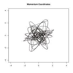
Figure 1(a-c) show the position and momentum coordinates for the first 1000 iterations and the scatter plots of MCMC samples drawn by HMC and Figure 1(d-f) exhibits those of MCMC samples generated by SAHMC. Scatter plots show that HMC cannot reach one of its three modes, whereas our SAHMC explores all parameter spaces. Figure 1(g-h) shows scatter plots of samples generated by 1st, 2nd and 3rd run of NUTS. As we can see, NUTS fails to visit all three modes in a few runs. In our simulation for Set 2, NUTS only visits all modes for five independent runs out of total 10 runs.

The weight terms, $\theta^{(t)}$, which are updated adaptively based on the frequencies of chain visits, help the SAHMC chains move more widely for both position and momentum coordinates so that it can explore more sample spaces while maintaining the efficiencies of HMC. Therefore, our SAHMC method performs much better than HMC and NUTS when our target density has multi-mode.

4.2 High-dimensional Multimodal Distributions

To investigate the performance of SAHMC in high-dimensional multimodal distributions, we consider an equal mixture of eight $d$-dimensional Gaussians previously discussed by Tak et al. (2018). The target distribution is

$$\pi(x)\propto\sum_{j=1}^{8}\exp\left(-0.5(x-\mu_{j})^{T}(x-\mu_{j})\right),$$ (17)

where $x=(x_{1},x_{2},\ldots,x_{d})^{T}$ and $\mu_{j}$ are determined by setting their first three coordinates to the eight vertices of a cube with edge length 10. The remaining coordinates are filled by alternating $0$ and $10$:

$$\mu_{1} =(10,10,10,0,10,0,10,\ldots,0,10),$$

$$\mu_{2} =(0,0,0,10,0,10,0,\ldots,10,0),$$

$$\mu_{3} =(10,0,10,0,10,0,10,\ldots,0,10),$$

$$\mu_{4} =(0,10,10,0,10,0,10,\ldots,0,10),$$

$$\mu_{5} =(0,0,10,0,10,0,10,\ldots,0,10),$$

$$\mu_{6} =(0,10,0,10,0,10,0,\ldots,10,0),$$

$$\mu_{7} =(10,0,0,10,0,10,0,\ldots,10,0),$$

$$\mu_{8} =(10,10,0,10,0,10,0,\ldots,10,0).$$

We will demonstrate that SAHMC efficiently explore a multimodal high-dimensional distribution in equation 17 with the five values of $d\in\{3,5,7,9,11\}$. We compare SAHMC to vanilla HMC and NUTS.

For each $d$, HMC and SAHMC share the same the leapfrog step-size, $\epsilon$ and leapfrog steps, $L$, which are listed in 2. These values are chosen so that the acceptance rate is between $0.4$ and $0.7$. We set the sample space was partitioned with equal energy bandwidth $\Delta u=2$ into the following subregions: $E_{1}=\{{\bf x}:-\log p({\bf x})<u_{1}\}$, $E_{2}=\{{\bf x}:0\leq-\log p({\bf x})<u_{1}+2\}$, $\cdots$, and $E_{m}=\{{\bf x}:-\log p({\bf x})>u_{1}+2(m-1)\}$. The values of $u_{1}$ and $m$ for each $d$ are listed in 2. The number of iterations are chosen so that each sampler produce approximately equal computation time. Other configurations of samplers follow those in Section 4.1.

Table 2: High-dimensional multimodal distributions: Configurations of SAHMC and HMC include the leapfrog step-size ($\epsilon$), leapfrog steps ($L$), the minimum energy level ($u_{1}$), and the number of energy partitions ($m$).

d	$\epsilon$	$L$	$u_{1}$	$m$
3	0.9	1	8.0	6
5	0.25	3	8.0	10
7	0.25	3	8.0	14
9	0.25	3	8.0	18
11	0.25	3	8.0	22

For each $d$, we run SAHMC ten times to obtain ten chains each of length 1,000,000, discarding the first 200,000 iterations of each chain as burn-in. As $d$ increases, SAHMC requires more evaluations because it is more difficult to find a proposal that increases the density in the forced uphill transition.

We use two measures to evaluate each method. The first is $N_{dis}$, the average number of the unknown modes that are discovered by each chain. A mode $\mu_{j}$ is tagged as uudiscovered” when at least one sample has $\mu_{j}$ as the closest mode measured by the Euclidean distance. The second is $F_{err}=\sum\nolimits_{i=1}^{10}\sum\nolimits_{j=1}^{8}|F_{i,j}-1/8|/80$, the average frequency error rate Tak et al. (2018), where $F_{i,j}$ is the proportion of iterations in chain $i$ whose closest mode is $\mu_{j}$.

Table 3 summarizes the results, and shows that SAHMC is never worse than NUTS in terms of $N_{dis}$ and $F_{err}$ regardless of dimension. HMC’s $F_{err}$ is only a bit smaller than that of SAHMC at $d=3$ but deteriorates much faster than SAHMC’s and NUTS’s. Eight modes get more isolated in terms of Euclidean distance as the dimension Hence, there are more obstacles for samplers to travel across modes for high-dimension. In high-dimensions, SAHMC performs much efficiently by sampling across high energy barriers between multiple modes.

Table 3: High-dimensional multimodal distributions: Comparison of SAHMC, HMC, and NUTS. The simulation results include the number of iterations; the burn-in size; $N_{dis}$ = the average number of modes discovered by each chain; and $F_{err}=\sum\nolimits_{i=1}^{10}\sum\nolimits_{j=1}^{8}|F_{i,j}-1/8|/80$, where $F_{i,j}$ is the proportion of iterations in chain $i$ whose closest mode is $\mu_{j}$.

d	Kernel	Length of a chain (burn-in size)	CPU time (s)	$N_{dis}$	$F_{err}$
3	SAHMC	1,000,000 (200,000)	2.98	8	0.0030
	HMC	1,000,000 (200,000)	3.01	8	0.0024
	NUTS	555,000 (110,000)	3.72	8	0.0624
5	SAHMC	1,000,000 (200,000)	5.24	8	0.0050
	HMC	1,000,000 (200,000)	5.22	8	0.0246
	NUTS	687,500 (137,500)	5.83	8	0.0655
7	SAHMC	1,000,000 (200,000)	5.59	8	0.0081
	HMC	1,000,000 (200,000)	5.63	4.4	0.1248
	NUTS	500,000 (100,000)	5.90	8	0.0955
9	SAHMC	1,000,000 (200,000)	5.87	8	0.0265
	HMC	1,000,000 (200,000)	5.83	4	0.1250
	NUTS	375,000 (075,000)	6.10	8	0.1036
11	SAHMC	1,000,000 (200,000)	6.11	8	0.0431
	HMC	1,000,000 (200,000)	6.13	4	0.1250
	NUTS	350,000 (070,000)	7.26	8	0.1082

4.3 Sensor Network Localization

We illustrate the advantage of SAHMC using a sensor network localization problem previously discussed by Tak et al. (2018); Ahn et al. (2013); Ihler et al. (2005). This problem is known to produce a high-dimensional and multimodal joint posterior distribution. Following the experiment setting in Tak et al. (2018), we assume N sensors are scattered in a planar region with 2d locations denoted by $\{x_{t}\}_{t=1}^{N}$. The distance between a pair of sensors $(x_{t},x_{u})$ is observed with a probability $\exp(-0.5||x_{t}-x_{u}||^{2}/R^{2})$, and the observed distance between $x_{t}$ and $x_{u}$, denoted by $Y_{t,u}$, follows a Gaussian distribution with mean $||x_{t}-x_{u}||$ and standard deviation $\sigma$. Independent bivariate Gaussian prior distributions with mean $(0,0)$ and covariance matrix $10^{2}\times I_{2}$ are assumed for $x_{t}$’s. Given a set of observations $\{y_{t,u}\}$, a typical task is to infer the posterior distribution of all the sensor locations. Following Tak et al. (2018), we choose $N=4$, $R=0.3$, $\sigma=0.02$ and add two additional sensors with known locations. The locations of the 4 sensors form a multimodal distribution of 8 dimensions.

For both HMC and SAHMC, we set the leapfrog step-size, $\epsilon=0.02$, and leapfrog steps, $L=3$. For SAHMC, the sample space was partitioned with equal energy bandwidth $\Delta u=2$, the minimum energy level $u_{1}=-4$ and the number of partitions $m=19$. We implemented SAHMC and HMC for 2,000,000 iterations with the first 400,000 as burn-in, resulting in 106 seconds computation time. For a fair comparison in terms of computation time, we implemented NUTS for 400,000 iterations with the first 80,000 as burn-in, resulting in 102 seconds computation time. All other configurations of samplers follow those described in Section 4.1.

Figure 2 shows scatter plots of the posterior samples of each sensor location obtained by the three samplers. The dashed lines indicate the coordinates of the true location. We can see that HMC and NUTS fail to visit one of the modes; whereas, SAHMC frequently visits this mode and generate enough samples from it.

Figure 2: Scatterplots of the posterior sample of each sensor location obtained by SAHMC, HMC and NUTS. The coordinates of the true location are denoted by dashed lines.

5 An Application to Neural Networks

Feed-forward neural networks, which are also known as multiple layer perceptrons (MLP), are one of well-known models in machine learning community (Schmidhuber, 2012). Given a group of connection weights ${\bf z}=(\alpha,\beta)$, the MLP can be written as

$$f\Big{(}{\bf x}_{i}\mid{\bf z}\Big{)}=\varphi\bigg{(}\alpha_{0}+\sum_{k=1}^{N}\alpha_{k}\varphi\Big{(}\beta_{k0}+\sum_{j=1}^{p}\beta_{kj}x_{ij}\Big{)}\bigg{)},$$ (18)

where $N$ is the number of hidden units, $p$ is the number of input units, ${\bf x}_{i}=\big{(}x_{i1},\cdots,x_{ip}\big{)}$ is the $i$-th input patterns, and $\alpha_{k}$, and $\beta_{kj}$ are the weights on the connections from the $k$-th hidden unit to the output unit, from the $j$-th input unit to the $k$-th hidden unit, respectively. The function $\varphi$ is the activation function of the hidden and output units. Popular choices of $\varphi(\cdot)$ include the sigmoid function, the hyperbolic tangent function, and the rectified linear unit (ReLU).

(a) SAHMC	(b) HMC

Figure 3: An example of trace plots.

There have been multiple studies regarding computational aspects of Bayesian neural network models via MCMC algorithms (Andrieu et al., 2000; Lampinen and Vehtari, 2001)but their practical performance were questioned due to the highly correlated parameters on posterior space. Alternatively, in Neal (2012) the HMC was used to sample the weight parameters, improving the convergence of the MCMC chain. However, the highly multimodal nature of the posterior distribution of the MLP still hinders the practical implementation of neural network models. To solve this issue, we apply the SAHMC to neural network models, and consider simulated datasets to examine the capacity of the SAHMC to efficiently explore the multimodal posterior space.

A Simulation Study

We consider a simple regression settings with one predictor for one-layered feedforward neural network, and we generate the data from $y_{i}=f_{0}(x_{i})+\epsilon_{i}$, where the true function $f_{0}(x)=3\varphi(x-1.5)-\varphi(x+1)-3\varphi(x-1)+2\varphi(x)$ with the ReLU function $\varphi(x)=\max\{0,x\}$, and $\epsilon_{i}\sim N(0,1)$ for $i=1,\dots,n$. We independently replicates 200 simulated data sets and use SAHMC and HMC to sample from the posterior distribution of the connection weights.

For both HMC and SAHMC, we set the leapfrog step-size, $\epsilon=0.005$, and leapfrog steps, $L=25$. To run SAHMC, we set the sample space ${\cal X}=[-10^{100},10^{100}]^{2}$ to be compact and it was partitioned with equal energy bandwidth $\Delta u=2$ into the following subregions: $E_{1}=\{{\bf x}:-\log p({\bf x})<460\}$, $E_{2}=\{{\bf x}:460\leq-\log p({\bf x})<462\}$, $\cdots$, and $E_{51}=\{{\bf x}:-\log p({\bf x})>560\}$. Additionally, we set $t_{0}=1000$ and the desired sampling distribution, $\bm{\pi}$ to be uniform for SAHMC. Both HMC and SAHMC were independently run and each run consists of 55,000 iterations, where the first 5,000 iterations were discarded as a burn-in process. All initial points are randomly selected for all simulations.

To measure the performance of each procedure, we consider a Posterior risk of $f(x|{\bf z})$, that is $\sum_{i=1}^{n}\mathbb{E}_{\bf z\mid y}\left[\{f_{0}(x_{i})-f(x_{i}\mid{\bf z})\}^{2}\right]$, where $\mathbb{E}_{\bf z\mid y}$ is the expectation operator with respect to the posterior distribution of ${\bf z}$, and we also consider the ESS. We also report the minimum energy found by the SAHMC and the HMC and the proportion of the cases where the SAHMC procedure finds the smaller energy region than the energy found by the other procedure. The results are averaged over 200 replicated data sets.

Method	Posterior Loss	ESS (min, med, max)
HMC	0.112	(4.1, 40.3, 282.7)
SAHMC	0.077	(8.3, 184.9, 335.8)

Table 4: Results of the Simulation Study: Comparison of SAHMC and HMC

Table 4 summarizes the performance of the SAHMC and the HMC shows that the posterior expectation of $L_{2}$ loss from the regression function evaluated by the SAHMC achieves a smaller than that from the HMC. The median ESS of the SAHMC is about 4.5 times larger than that of the HMC.

In Figure 3, we provide an example of the trace plot of a SAHMC chain and a HMC chain for a simulated data set. This example illustrates how different the Markov chains of SAHMC and HMC are. The SAHMC chain explores all energy level between 503 and 571, while the HMC chain searches only narrower energy level between 509 to 541. This shows the capacity of SAHMC in escaping local maxima of the posterior distribution and exploring wider region of the posterior space.

Pima Indians Diabetes Classification

We consider a real data set that contains 768 records of female Pima Indians, characterized by eight physiological predictors and the presence of diabetes (Smith et al., 1988). We model the data by an artificial neural network (ANN) of a single layer equipped with 25 hidden nodes. The ANN is trained using SAHMC and HMC on a randomly selected $90\%$ of samples, and the out-sample prediction error was evaluated over $10\%$ of the other samples. We replicates this procedure 100 times and report the test error, ESS, and the average of minimum energy values found by each procedure. All other algorithm settings are same except the energy partitions: $E_{1}=\{{\bf x}:-\log p({\bf x})<290\}$, $E_{2}=\{{\bf x}:290\leq-\log p({\bf x})<292\}$, $\cdots$, and $E_{36}=\{{\bf x}:-\log p({\bf x})>360\}$.

Method	Test Error	ESS (min, med, max)	min.Energy
HMC	0.383	(1.7,4.0,24.9)	294.90
SAHMC	0.265	(4.4,15.0,34.5)	289.13

Table 5: Pima Indians Diabetes Data Set

Table 5 shows that the SAHMC algorithm collects more effective samples and achieves a smaller test error compared to the HMC. The average of the minimum energy searched by the SAHMC is also 5.77 lower than that found by the HMC.

6 Concluding Remarks

In this paper, we propose a new algorithm which generates samples from multimodal density under the HMC framework. Because SAHMC can adaptively lower the energy barrier, our proposed algorithm, SAHMC can explore the rugged energy space efficiently. We compare the results of SAHMC with those of HMC and NUTS and show that SAHMC works more efficiently when there exists multiple modes in our target density, especially in high dimension.

RMHMC (Girolami and Calderhead, 2011) can be easily combined with SAHMC by replacing the fixed mass matrix, $\bf M$ with a position dependent expected Fisher information matrix $\bf M(\bf x)$. We have implemented this algorithm and observed some performance gain in terms of ESS per iteration. However, $\bf M(\bf x)$ should be updated at each iteration using the fixed point iteration, which poses a computational bottleneck. As a result, its performance per CPU time is not as good as that of SAHMC.

One of the main issues that arise when HMC is used, is parameter tuning of the algorithm (e.g. the mass matrix, $\bf{M}$, $\epsilon$ and $L$ in the leapfrog integrator). A choice of these parameters is essential for good convergence of the sampler. Combining HMC with SAMC, our proposed sampler shows its ability to fully explore complex target distributions without much efforts to tuning these parameters to make HMC work. It should be noted that HMC samplers using the same parameters show poor convergence.

One difficulty in the application of SAHMC is how to set up the boundary of sample space partition. One approach we can take to overcome this difficulty is running our SAHMC with two stages. At the first stage, we run HMC with a few hundreds iterations, and then, run SAHMC with the range of the sample space determined by the results of the first stages.

References

- Ahn et al. (2013) Ahn, S., Y. Chen, and M. Welling (2013, April). Distributed and Adaptive Darting Monte Carlo through Regenerations. In Artificial Intelligence and Statistics, pp. 108–116.
- Andrieu et al. (2000) Andrieu, C., N. De Freitas, and A. Doucet (2000). Reversible jump MCMC simulated annealing for neural networks. In Proceedings of the Sixteenth conference on Uncertainty in artificial intelligence, pp. 11–18. Morgan Kaufmann Publishers Inc.
- Andrieu et al. (2005) Andrieu, C., E. Moulines, and P. Priouret (2005). Stability of stochastic approximation under verifiable condition. SIAM Journal of Control and Optimization 44, 283–312.
- Benveniste et al. (1990) Benveniste, A., M. Métivier, and P. Priouret (1990). Adaptive Algorithms and Stochastic Approximations. New York, NY: Springer-Verlag.
- Betancourt et al. (2014) Betancourt, M., S. Byrne, S. Livingstone, and M. Girolami (2014). The geometric foundations of Hamiltonian Monte Carlo. arXiv:1410.5110v1.
- Carpenter et al. (2017a) Carpenter, B., A. Gelman, M. D. Hoffman, D. Lee, B. Goodrich, M. Betancourt, M. Brubaker, J. Guo, P. Li, and A. Riddell (2017a). Stan: A probabilistic programming language. Journal of Statistical Software 76.
- Carpenter et al. (2017b) Carpenter, B., A. Gelman, M. D. Hoffman, D. Lee, B. Goodrich, M. Betancourt, M. Brubaker, J. Guo, P. Li, and A. Riddell (2017b, January). Stan: A Probabilistic Programming Language. Journal of Statistical Software 76(1), 1–32. Citation Key Alias: carpenter_stan_2017.
- Duane et al. (1987) Duane, S., A. D. Kennedy, B. J. Pendleton, and D. Roweth (1987). Hybrid Monte Carlo. Physics Letters B 195, 216–222.
- Durmus et al. (2017) Durmus, A., E. Moulines, and E. Saksman (2017). On the convergence of Hamiltonian Monte Carlo. arXiv:1705.00166.
- Fok et al. (2017) Fok, R., A. An, and X. Wang (2017, September). Optimization assisted MCMC. arXiv:1709.02888 [cs, stat].
- Gilks et al. (1998) Gilks, W. R., R. O. Roberts, and S. K. Sahu (1998). Adaptive Markov chain Monte Carlo through regeneration. Journal of the American Statistical Association 93, 1045–1054.
- Girolami and Calderhead (2011) Girolami, M. and B. Calderhead (2011). Riemann manifold Langevin and Hamiltonian Monte Carlo methods. Journal of the Royal Statistical Society: Series B 73, 123–214.
- Henderson and Goggans (2019) Henderson, R. W. and P. M. Goggans (2019, December). TI-Stan: Model Comparison Using Thermodynamic Integration and HMC. Entropy 21(12), 1161. Number: 12 Publisher: Multidisciplinary Digital Publishing Institute.
- Hoffman and Gelman (2014) Hoffman, M. D. and A. Gelman (2014). The No-U-Turn sampler: Adaptively setting path lengths in Hamiltonian Monte Carlo. Journal of Machine Learnning Research 15, 1593–1623.
- Ihler et al. (2005) Ihler, A., J. Fisher, R. Moses, and A. Willsky (2005, April). Nonparametric belief propagation for self-localization of sensor networks. IEEE Journal on Selected Areas in Communications 23(4), 809–819.
- Lampinen and Vehtari (2001) Lampinen, J. and A. Vehtari (2001). Bayesian approach for neural networks-review and case studies. Neural networks 14(3), 257–274.
- Lan et al. (2014) Lan, S., J. Streets, and B. Shahbaba (2014). Wormhole Hamiltonian monte carlo. In Proceedings of Twenty-Eighth AAAI Conference on Artificial Intelligence, Palo Alto, CA, pp. 1953–1959. AAAI Press.
- Liang (2007) Liang, F. (2007). Annealing stochastic approximation Monte Carlo for neural network training. Machine Learning 68, 201–233.
- Liang (2009) Liang, F. (2009). Improving SAMC using smoothing methods: Theory and applications to Bayesian model selection problems1. The Annals of Statistics 37(5B), 2626–2654.
- Liang et al. (2007) Liang, F., C. Liu, and R. J. Carroll (2007). Stochastic approximation in Monte Carlo computation. Journal of the American Statistical Association 102, 305–320.
- Livingstone et al. (2016) Livingstone, S., M. Betancourt, S. Byrne, and M. Girolami (2016). On the geometric ergodicity of Hamiltonian Monte Carlo. arXiv:1601.08057.
- Neal (2010) Neal, R. (2010). Mcmc using hamiltonian dynamics. In S. Brooks, A. Gelman, G. Jones, and X.-L. Meng (Eds.), Handbook of Markov chain Monte Carlo, pp. 113–162. New York: Chapman & Hall.
- Neal (2012) Neal, R. (2012). Bayesian learning for neural networks, Volume 118. Springer Science & Business Media.
- Nishimura and Dunson (2016) Nishimura, A. and D. Dunson (2016). Geometrically tempered Hamiltonian Monte Carlo. arXiv:1604.00871.
- Robbins and Monro (1951) Robbins, H. and S. Monro (1951). A stochastic approximation method. The Annals of Mathematical Statistics 22, 400–407.
- Schmidhuber (2012) Schmidhuber, J. (2012). Deep learning in neural networks: An overview. Neural Networks 61, 85–117.
- Shahbaba et al. (2013) Shahbaba, B., S. Lan, W. O. Johnson, and R. M. Neal (2013). Split hamiltonian monte carlo. Statistics and Computing 24, 339–349.
- Smith et al. (1988) Smith, J. W., J. Everhart, W. Dickson, W. Knowler, and R. Johannes (1988). Using the ADAP learning algorithm to forecast the onset of diabetes mellitus. In Proceedings of the Annual Symposium on Computer Application in Medical Care, pp. 261. American Medical Informatics Association.
- Sohl-Dickstein et al. (2014) Sohl-Dickstein, J., M. Mudigonda, and M. DeWeese (2014). Hamiltonian monte carlo without detailed balance. In Proceedings of the 31st International Conference on Machine Learning, Volume 32, pp. 719–726.
- Tak et al. (2018) Tak, H., X.-L. Meng, and D. A. van Dyk (2018, July). A Repelling-Attracting Metropolis Algorithm for Multimodality. Journal of Computational and Graphical Statistics 27(3), 479–490.