Turbulence, Gravity, and Multimessenger Asteroseismology
© John Ryan Westernacher-Schneider, October, 2018)
Abstract
Turbulence, Gravity, and Multimessenger Asteroseismology
John Ryan Westernacher-Schneider, MSc
University of Guelph, 2018
Part IA: We present numerical measurements of relativistic scaling relations in -dimensional conformal fluid turbulence, which perform favourably over their non-relativistic versions. As seen with incompressible turbulence in past studies, we find that the energy spectrum exhibits scaling rather than the Kolmogorov/Kraichnan expectation of .
Part IB: We compute the fractal dimension of a turbulent anti-deSitter black brane reconstructed from boundary fluid data using the fluid-gravity duality. Our value of is consistent with the upper bound , resolving a recent claim that . We describe how to covariantly define the fractal dimension of spatial sections of the horizon, and we speculate on assigning a ‘bootstrapped’ value to the entire horizon.
Part II: We report progress implementing a fluid code with post-Newtonian (PN) gravity in spherical symmetry. The PN formalism couples a fluid, its self-gravity, and a black hole via elliptic equations. This eliminates radiative modes, allowing larger time steps, which is helpful for studying systems with very long time scales, eg. tidal disruption events.
Part III: Asteroseismology of rotating core-collapse supernovae is possible with a multimessenger strategy. We show an , , , Hz mode of the core is responsible for emission in gravitational waves and neutrinos. The angular harmonics of the neutrino emission is consistent with the mode energy around the neutrinospheres, where km. Thus, neutrinos carry information about the mode in the outer region of the core, whereas gravitational waves probe the deep inner core km.
To my mother, whose patience, strength, and love knows no bounds;
and my father, who is sorely missed.
Acknowledgments
It is a pleasure to thank my advisor, Luis Lehner, for his guidance and support in the completion of this thesis. I would also like to thank the remainder of my committee members Eric Poisson, Erik Schnetter, and Alexandros Gezerlis for their support.
Also, thank you to the following: Michael Waite for detailed discussions on dealiasing and other matters, Guido Boffetta for sharing unpublished statistical values from the study [1], Gregory Falkovich for an interesting discussion on turbulence, Neil Cornish, Zachary Vernon, Robie Hennigar, and Eric Poisson for helpful discussions pertaining to my fractal dimension work.
I am especially indebted to my collaborator Evan O’Connor who performed all of the core-collapse supernova simulations in Part (III) of this dissertation. That work was initiated in the summer of 2017 at the Niels Bohr Institute, during the Kavli Summer Program in Astrophysics; I would like to thank the hosts for their hospitality, and the organizers for running a great program.
| Notation Key | |||
|---|---|---|---|
| Symbol | Description | ||
| Number of spatial dimensions | |||
| (indices) | Spacetime indices | ||
| (indices) | Spatial indices | ||
| , , | Fluid 3-velocity | ||
| Fractal dimension, conserved relativistic rest mass density | |||
| Fluid 4-velocity | |||
| , , | Kinematic viscosity, friction coefficient, forcing strength, respectively (Part (IA)) | ||
| Stream function (Part (IA)), post-Newtonian potential (Part (II)) | |||
| , , | Rest mass density ( in Part (III)), specific internal energy, pressure, respectively | ||
| Total energy density (Parts (IA) & (IB)), rest mass density (Part (III)) | |||
| , | Vorticity in 2D, 3D, respectively | ||
| , | External force 3-vector | ||
| , | External force 4-vector, friction 4-vector, respectively | ||
| , | Average specific energy, palinstrophy, respectively | ||
| Isotropic specific energy spectrum | |||
| Average specific enstrophy | |||
| Spatial average, ensemble average | |||
| , | Average specific energy/enstrophy dissipated by viscosity, respectively | ||
| , , | Forcing, friction, and viscous length scales, respectively | ||
| Magnitude of wavevector | |||
| , | Isotropic specific spectral energy/enstrophy flux, respectively (Parts (IA) & (IB)) | ||
| , | Velocity difference in directions parallel and perpendicular to | ||
| Velocity structure function of order | |||
| , | Minkowski metric, general spacetime metric, respectively | ||
| Intrinsic metric of spacelike hypersurfaces | |||
| Determinant of general spacetime metric | |||
| Energy-momentum tensor | |||
| Kronecker delta | |||
| Speed of light and speed of sound, respectively | |||
| Lorentz gamma factor | |||
| , | Separation 3-vector | ||
| , , , | Conservative fluid variables (in addition to ) | ||
| , | Light-crossing time and linear box size, respectively | ||
| (indices) | transverse, longitudinal directions, respectively | ||
| , | Neutrino luminosity, neutrinosphere radius | ||
| Pre-collapse central rotation rate | |||
| , , | Electron, anti-electron, and heavy lepton neutrinos, respectively | ||
| , , , | Post-Newtonian metric potentials (Part (II)) | ||
| , | Auxiliary post-Newtonian variables (Part (II)) | ||
| Spherical harmonic | |||
| , , | Components of infinitesimal Eulerian displacement | ||
| Measure of eigenfunction match | |||
| Mode frequency | |||
| , , … | Fundamental mode and its overtones | ||
| , , … | Fundamental mode and its overtones | ||
Part IA Relativistic turbulence in dimensions
Executive summary
Scaling relations have been a central pillar of the statistical understanding of turbulence for many decades. They have found uses in astrophysics for example via size-linewidth relations, where the Doppler broadening of spectral lines from a turbulent cloud of matter is related to its size via a turbulent scaling relation. Extending these relations to the relativistic case is a logical next step, with recent progress being made in this direction. In this part, we present measurements of relativistic scaling relations in -dimensional conformal fluid turbulence from direct numerical simulations, in the weakly compressible regime. We analytically derived these scaling relations previously in [2] for a relativistic fluid; this work is a continuation of that study. We first explicitly demonstrate that the non-relativistic limit of these scaling relations reduce to known results from the statistical theory of incompressible Navier-Stokes turbulence. In simulations of the inverse-cascade range, we find the relevant relativistic scaling relation is satisfied to a high degree of accuracy. We observe that the non-relativistic versions of this scaling relation underperform the relativistic one in both an absolute and relative sense, with a progressive degradation as the rms Mach number increases from to . In the direct-cascade range, the two relevant relativistic scaling relations are satisfied with a lower degree of accuracy in a simulation with rms Mach number . We investigate the poorer agreement with further simulations of an incompressible Navier-Stokes fluid. Finally, as has been observed in the incompressible Navier-Stokes case, we show that the energy spectrum in the inverse-cascade of the conformal fluid exhibits scaling rather than the Kolmogorov/Kraichnan expectation of , and that it is not necessarily associated with compressive effects.
![[Uncaptioned image]](/html/1810.04594/assets/x1.png) Figure IA: Snapshots of vorticity from our simulations. See the text at the end of Part (IA) for details.
Figure IA: Snapshots of vorticity from our simulations. See the text at the end of Part (IA) for details.
Chapter 1 Introduction
Relativistic hydrodynamics has become a subject of increased interest in recent years. Beyond its relevance in astrophysical scenarios (e.g. [3, 4, 5, 6, 7]), it has become relevant to the description of quark-gluon plasmas (e.g. [8, 9]) and, through the fluid-gravity correspondence, it has found its way into the realm of fundamental gravity research [10, 11]. Intriguingly, this correspondence has revealed that gravity can exhibit turbulent behavior, and studies of its possible consequences are gaining interesting momentum [12, 13, 14, 15, 16]. The understanding of turbulence in any regime is a difficult task given its intrinsic complexity, and despite a long history of efforts in the subject, our knowledge of this rich phenomenon is still incomplete. Important headways into this subject have been made thanks to statistical analysis complemented with numerical simulations (e.g. [17, 18, 19, 20, 21]). Of particular interest is to understand the possible onset of turbulence, and especially to derive scaling relations in fully-developed scenarios, since those cases are amenable to a statistical description from which generic statements can be drawn and then tested numerically and observationally.
To date however, only limited attention has been placed on the relativistic turbulent regime, and most of what is known restricts to the behavior of turbulent, incompressible flows in the non-relativistic regime. There has been some work on the analytical front [22, 2, 23] and several numerical investigations [13, 24, 25, 2, 26, 27, 28, 29, 30, 31]. Because correlation functions can indeed be measured in relevant scenarios – perhaps even in quark-gluon plasma[32, 8, 33, 9, 34] – and interesting implications for the gravitational field follow from holography, it is of interest to further investigate relativistic turbulence.
In the current work we measure scaling relations in -dimensional relativistic conformal fluids in the weakly-compressible turbulent regime and compare them to the predictions in [2] and various limits thereof. The -dimensional case is especially relevant to draw intuition for related phenomena in -dimensional gravity with the help of the fluid-gravity correspondence (e.g. [12, 25, 16]). This work is largely a continuation and completion of [2], which contained a numerical study which was inconclusive at the time.
This part is organized as follows. Chapter (2) provides some background material, discussing both the inverse- and direct-cascade ranges that could ensue in fully-developed turbulence and, in particular, relevant scaling relations which we have measured. In Chapter (3) we provide details of our numerical implementations. This includes the use of a random external force to generate the turbulent flow, as well as considerations specific to simulating either a conformal fluid or an incompressible Navier-Stokes fluid. The equivalence between previously known results and the incompressible limit of the scaling relations derived in [2] is explicitly demonstrated. We give our results in Chapter (4), where our numerical measurements of the scaling relations derived in [2] are presented. In Chapter (5), we provide additional discussion and ancillary numerical results, including the demonstration of a energy spectrum in the inverse-cascade of a turbulent conformal fluid which is not due to compressive effects.
In this part, angle brackets will refer to ensemble averages. Letters at the beginning of the alphabet will represent spacetime indices , while letters in the middle of the alphabet will represent spatial indices . We follow Einstein summation convention. In the context of correlation functions, which often depend on two points and , we define . To avoid cumbersome notation, we denote quantities evaluated at with a prime (eg. ) and quantities evaluated at without one (eg. ). The metric signature is for our -dimensional setup.
Chapter 2 Background
We will make extensive connections with the work presented in [2], where specific scaling relations were derived analytically for -dimensional relativistic hydrodynamic turbulence. We will compare these relations with suitable limits in order to make contact with previously known results, as well as to gauge the importance of relativistic vs compressible contributions in our simulations of the specific case of a conformal fluid.
2.1 Incompressible non-relativistic limit of the scaling relations
In this section we explicitly demonstrate that the incompressible Navier-Stokes limit of the relativistic scaling relations presented in [2] can be written in terms of known results. We will use the particular form of a barotropic perfect fluid stress-energy tensor with equation of state , where is the pressure, is the energy density, and is the equation of state parameter. In doing so, we obtain incompressible counterparts to the relativistic scaling relations we measure in simulations, which act as a point of reference against which to gauge the relative performance of the relations derived in [2].
2.1.1 Inverse-cascade range
The first scaling relation, which is valid in the inverse-cascade range, reads [2]
| (2.1) |
where . For a perfect fluid, where , the scaling relation expands to
| (2.2) |
where is the Lorentz factor and is the spatial velocity (). In the extreme incompressible non-relativistic limit, and . Thus , and Eq. (2.2) becomes
| (2.3) |
where we have defined as the incompressible Navier-Stokes version of . Note that the second term on the left-hand side vanishes due to statistical isotropy, yielding the final result
| (2.4) |
Since Eq. (2.4) is the incompressible Navier-Stokes limit of the relativistic scaling relation in Eq. (2.1), they can be compared in the inverse-cascade range of relativistic or compressible turbulence in order to gauge their relative performance.
Notice one can also arrive at Eq. (2.4) using known results in the theory of -dimensional incompressible Navier-Stokes turbulence. In the derivations presented in [35], an intermediate result is displayed as
| (2.5) |
valid in the inverse-cascade range. Here, denotes a difference, i.e. . Expanding out the left-hand side of Eq. (2.5) and using statistical homogeneity yields
| (2.6) |
By incompressibility, the second term on the right-hand side is divergence-free. Thus, assuming isotropy and regularity at , it must vanish [36] (this argument will be used repeatedly in Sec. (2.1.2)). Therefore, Eq. (2.5) becomes
| (2.7) |
which is the incompressible non-relativistic limit we obtained in Eq. (2.4).
2.1.2 Direct-cascade range
The second relativistic scaling relation that we consider, which is valid instead in the direct-cascade range, reads [2]
| (2.8) |
where , , and . Note that is a random external force. In the incompressible non-relativistic limit, becomes proportional to the enstrophy dissipation rate [35], namely . Expanding the left-hand side of Eq. (2.8) and setting and as before, we obtain
| (2.9) | |||||
The second term on the right-hand side is proportional to the average vorticity, which vanishes by parity invariance. Thus Eq. (2.8) becomes
| (2.10) |
where the non-relativistic vorticity is . The left-hand side needs to be manipulated further in order to compare with standard results (e.g. [35]). First, notice that the ensemble average on the left-hand side expands under the product rule to
| (2.11) |
We can show that the second term on the right-hand side is zero as follows:
| (2.12) | |||||
where we used the identity in the first line. Again, isotropy and regularity at the origin will imply this vanishes, provided it is divergence-free [36]. Thus, we can compute its divergence and show that it vanishes:
| (2.13) | |||||
where we used incompressibility in the second and last lines. The relativistic scaling relation Eq. (2.8) thus reduces in the incompressible Navier-Stokes limit to
| (2.14) |
As before, this relation is equivalent to an intermediate standard result from [35], namely
| (2.15) |
To see this, expand the left-hand side and use statistical symmetries to obtain
| (2.16) |
and then note that the second term on the right-hand side vanishes by incompressibility, isotropy, and regularity at [36]. Thus Eq. (2.15) is the same as Eq. (2.14). Since Eq. (2.14) is the incompressible Navier-Stokes limit of Eq. (2.8), it can be compared in the direct-cascade range of relativistic or compressible turbulence in order to gauge their relative performance.
Finally, we demonstrate that the relativistic correlation derived in [2], which reads
| (2.17) |
also reduces to a known result in the incompressible non-relativistic limit. Note that the subscripts refer to the longitudinal () and transverse () directions, respectively. Once again, setting and yields
| (2.18) |
Since Eq. (2.18) is the incompressible Navier-Stokes limit of Eq. (2.17), they can also be compared in the direct-cascade of relativistic or compressible turbulence in order to gauge their relative performance.
Again, Eq. (2.18) can be obtained from standard results in [35]. The first intermediate result for the direct-cascade range that we use reads
| (2.19) |
Using statistical symmetries, the left-hand side expands to , and the second term vanishes due to incompressibility, isotropy, and regularity at the origin [36]. Thus, setting in Eq. (2.19), we obtain
| (2.20) |
We can eliminate the first term on the left-hand side using the well-known -law, also derived in [35] and valid in the direct-cascade range, . This substitution finally yields Eq. (2.18).
Chapter 3 Implementation
As stated, our goal is to explore scaling relations in conformal fluid turbulence. To ensure a clean inertial regime is established for the computation of the appropriate quantities, we include a driving source. Additionally, we ensure the numerical methods employed are consistent with the statistical properties of the flow we want to study. In this section we describe key aspects of our numerical implementation, beginning with general considerations in Sec. (3.1). Following this, we present specific considerations for the incompressible and relativistic cases in Secs. (3.2) and (3.3), respectively.
3.1 General considerations
3.1.1 Stochastic Runge-Kutta integrator
In order to implement a random white noise force in a simulation, a special integration algorithm must be used. Based on the work of Honeycutt [37], we use a second-order Stochastic Runge-Kutta algorithm (SRKII). The Gaussian random force we use, defined later in Eq. (3.2), is homogeneous, which means the average and variance of the force at every point in space is the same. Thus the prescription described in [37] is applied to each real space point, producing control over the injection rates in an aggregate sense.
3.1.2 Pseudorandom number generation
The random force we employ requires pseudorandom number generation at every time step. For this purpose, we implement the Intel MKL Vector Statistical Library. In particular, we use the Mersenne Twister 111With BRNG parameter VSL_BRNG_MT19937 [38] and block-splitting for parallel applications [39]. We have checked that the energy spectrum in steady-state is unaffected by the choice of random number generator by comparing the Mersenne Twister (VSL_BRNG_MT19937) and the 59-bit multiplicative congruential generator (VSL_BRNG_MCG59). We also checked that the output of our code is system-independent [39] by running it on two independent clusters.
3.1.3 Defining an injection length scale
In studies of turbulence, the energy/enstrophy injection and scale play a crucial role in establishing and identifying particularly relevant dynamical ranges. One can define an injection length scale associated with the external force in terms of the injection rates of energy and enstrophy as follows. Given Kraichnan-Batchelor [40] scaling of the energy spectrum in the inverse and direct cascades, , , respectively, one can take the injection scale to be the wavenumber at which transitions between these two scalings. Thus, set and solve to find . This definition will accurately represent the injection scale up to a numerical factor of order , so long as the energy spectrum transitions between these two behaviours over a short range of wavenumbers.
3.2 Incompressible case
3.2.1 Formulation
In the incompressible Navier-Stokes case in D, the entire dynamics is determined by a single pseudo-scalar quantity, the vorticity . Thus, it is computationally more efficient to evolve the vorticity equation directly, rather than the components of the velocity. We write the vorticity equation in “flux-conservative form”,
| (3.1) |
where is the random force defined in the next section, and the dissipative term on the right-hand side is often referred in the turbulence literature as “hyperviscosity of order ”. Hyperviscosity is frequently used in simulations of an incompressible Navier-Stokes fluid [20], since it limits the range of scales over which dissipation is active (yielding wider inertial ranges for a given grid resolution).
3.2.2 Random force and injection rates
The external force appears as , and we wish to construct directly with the appropriate statistical properties. Given a Gaussian random force with a two-point correlation in real space given by
| (3.2) |
for some function , the injection rate of enstrophy will be given by [41], owing to the delta function (i.e. white noise) and to the choice of Gaussian randomness. Ignoring the temporal part of the correlation, we have in Fourier space
| (3.3) |
where reality of the force in real space requires .
In order to specify the enstrophy injection rate , we use a rescaling strategy as follows. First, define two random scalar fields , , with zero average and unit variance at all wavenumbers, and set . We first seek an isotropic rescaling that gives the profile of Eq. (3.3) up to a constant factor. Under this rescaling, , so the zero average is unchanged but the variance transforms to . Thus,
| (3.4) | |||||
Thus choosing gives the desired spatial profile up to a constant factor. To fix the enstrophy injection rate (as ), we seek a second rescaling with constant determined as follows. As it stands, Eq. (3.4) will produce an enstrophy injection rate given by half of its inverse Fourier transform evaluated at ,
| (3.5) |
Under the second rescaling, Eq. (3.4) becomes . Thus the appropriate rescaling is
| (3.6) |
If one wishes instead to specify the energy injection rate, simply note that for a solenoidal force , we have the spatial part of Eq. (3.2) given by
| (3.7) | |||||
So by solving the Poisson equation one finds the energy injection rate from the relation . The rescaling factor can be chosen appropriately in this case. Extracting these a priori injection rates of energy and enstrophy allows one to define an injection length scale as per Sec. (3.1.3).
For our incompressible simulations of the direct-cascade we use a ‘rectangular’ profile, namely in a narrow range of wavenumbers around , zero otherwise.
3.2.3 Dealiasing
The Navier-Stokes equation has a quadratic nonlinearity. Thus, two wavenumbers , can interact to populate a third wavenumber . Since we have a finite range of scales resolved in any simulation, could exceed the largest resolved wavenumber, and thus would become represented on the grid as a lower wavenumber (where is the grid resolution). In this case, we say has been aliased. Prescriptions exist to avoid such aliasing errors. For a quadratically nonlinear term , if we filter out all wavenumber modes with in and prior to multiplication, then filter in the same manner, we will eliminate all aliasing errors. Such a prescription is known as the -dealiasing rule, since one retains of the domain in Fourier space. Analogous dealiasing rules exist for higher-order nonlinearities, with less and less of the domain being retained as the order increases. Thus, full dealiasing becomes computationally prohibitive for higher-order nonlinearities, such as for a relativistic fluid flow.
3.3 Relativistic conformal fluid case
3.3.1 Formulation
The system of equations is given by and the conformal perfect fluid stress-energy tensor , which uses the conformal equation of state in dimensions. Defining the conservative variables as , they appear in terms of the primitive variables as
| (3.8) |
where is the spatial velocity and is the Lorentz factor. In terms of these variables, the equations of motion appear in flux-conservative form as
| (3.9) | |||||
| (3.10) |
We use finite differences to discretize the derivatives, with RK4 in space and SRKII (see Sec. (3.1.1)) in time. The system is damped at short wavelengths using a 4th-order dissipation scheme discussed in Sec. (3.3.3).
3.3.2 Random force and injection rates
We choose the Gaussian white-noise force to be divergence-free by deriving it from a stream function , . Thus, numerically we build directly in the manner described in Sec. (3.2.2). For simulations of the inverse-cascade, we choose
| (3.11) |
where is the characteristic length scale of the correlation, and [2] is a constant. One can verify the equality by applying the 2-dimensional Laplacian to Eq. (3.11), then noting that the spatial part of , written as , is given by and [2]. In the weakly compressible regime, is approximately the injection rate of , whereas in the incompressible regime it fixes the Newtonian kinetic energy injection rate.
For simulations of the direct-cascade, we instead choose
| (3.12) |
3.3.3 Dealiasing
As alluded to in Sec. (3.2.3), in the relativistic case a full dealiasing is computationally prohibitive. Since the computation of the velocity from the conservative hydrodynamic variables, followed by the computation of the flux, amounts to forming a product of up to fields, there is a quintic nonlinearity. In the weakly-compressible regime, however, a -dealiasing rule would likely eliminate a satisfactory amount of aliasing, since the density and Lorentz factor have a small amount of power at all wavenumbers . However, in a future study we wish to explore the strongly compressible and ultrarelativistic regimes where a -rule would be inadequate. Thus we opt instead to use a 4th-order numerical dissipation scheme to suppress large wavenumber modes (since we want to explore the suitability of alternative dealiasing strategies for that future study) and employ a sufficiently high resolution (so that possibly spurious effects stay mainly confined at very high frequencies). For a variable , this scheme amounts to including a term on the right-hand side of its evolution equation, where is the strength of the dissipation. It is numerically convenient to write this term as and control the dissipation strength , as its magnitude will be closer to and the dissipation length scale will move with the resolution [42].
Chapter 4 Results
In all simulations we use periodic boundary conditions with a box size of and resolution of , with a variable step size determined by a CFL condition [43]. This resolution has proven quite adequate for studying correlation functions in both the inverse-cascade (eg. [1]) and direct-cascade (eg. [44, 45]) in incompressible fluid turbulence. We find it is also adequate for the weakly compressible regime studied here, since we have obtained the same inverse-cascade range spectral slope with .
The time scale over which a turbulent flow is presumed to erase knowledge of its initial conditions is the large-eddy turnover time, which has various interpretations in the literature. Borue [46] estimates it as , where is the root-mean-squared vorticity. More generally, we have where is the scale of the largest eddies and is a characteristic speed at that scale. is estimated as , where is the infrared “cutoff” ( largest energy-containing scale), and we estimate as the root-mean-square of the velocity. In our simulations, these time scales will be quoted for reference.
Averages will be computed over time, or over independent simulations, or both. The adequacy of the sample sizes is gauged via comparison of the average with the statistical error , where is the sample standard deviation and is the sample size. For example, a correlation function will have an ensemble of values for each , and is computed as the standard deviation of that collection of values.
4.1 Inverse-cascade simulations
We simulate the inverse-cascade of a -dimensional conformal fluid with an external force described by Eq. (3.11), and an injection scale defined by , as in Sec. (3.1.3). We consider three cases with the numerical dissipation strength given by (so as to compare results among them) and when quoting properties of each case we will present them in this order. Since the force is somewhat broadband, it has power in the dissipation range of scales. Thus, decreasing the dissipation strength is enough to increase the energy growth rate, and thus the rms Mach number of the flow, , where is the sound speed ( of the speed of light, in our case). Statistical quantities are averaged over ensembles of independent simulations, as well as averaged over an interval of time after the energy passes and before it reaches the box size. Table (4.1) contains various parameters of the flows, as well as the sample sizes for the joint average over an ensemble and over time.
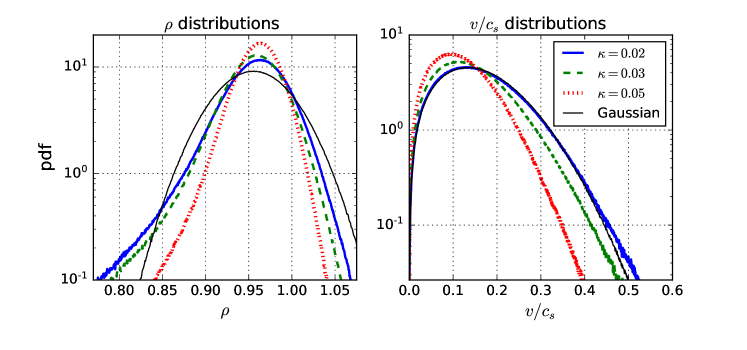
In Fig. (4.1) we characterize the flows by presenting the probability distributions functions (pdfs) of the energy density and Mach number. The pdfs are observed to widen as the energy growth rate increases, as one would expect. For comparison, in both cases we also plot Gaussian distributions (black, dashed) with average and standard deviation matched to the data from the case. The Gaussian provides a good fit to the Mach number pdf (although with a slight hint of non-Gaussianity in the tail), whereas the energy density pdf exhibits a stronger, exponential tail towards smaller values.
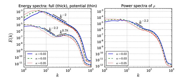
In Fig. (4.2) (Left) we display the angle-averaged Newtonian kinetic energy spectra (both the full spectrum and the potential part, obtained by projecting the velocity onto in Fourier space). We observe a steepening of the inertial range scaling towards , which we note is steeper than the Kolmogorov/Kraichnan power law of . The spectra are not changed significantly () by instead using density-weighted velocities or , the former having been suggested in the -dimensional context in [47] to restore Kolmogorov/Kraichnan scaling from the observed spectral exponent of . The spectrum of the potential component of the velocity exhibits a bump beginning at , with scaling of and on either side. Such a bump towards large is commonly observed in spectra in simulated compressible flows in dimensions, eg. [24, 47, 19, 48], and is attributed in those cases to an artefact of high-order numerical dissipation known as the bottleneck effect [49]. This effect has also been observed in simulated compressible 2D flows which exhibit transfer of energy to small scales [50]. The bump we observe in Fig. (4.2) is likely due to the same effect, although we cannot make a conclusive statement since we have not performed the specific resolution studies necessary to do so, nor have we used dissipation of a different order. The late-time spectra obtained from our simulations of the direct-cascade (not shown) also exhibit such a bump, and in that case we note that reducing the time step by half does not change the bump perceptibly.
With regard to the full inverse-cascade spectra in Fig. (4.2) (Left), it is worth noting that there is no large-scale friction. In [51], it was shown that the presence of large-scale friction can affect the inertial range spectrum in the incompressible Navier-Stokes case. In the same study it was also shown that measurements of the inertial range spectrum are not reliable without a sufficiently resolved enstrophy cascade (, where is defined as ). We do not have the direct-cascade range resolved to this degree in Fig. (4.2) (). The approach of the full spectrum towards is generally expected for compressible turbulence in both dimensions (see eg. [48]) and dimensions (see eg. [52]), although usually for much larger Mach numbers than our current simulations. With that said, -dimensional conformal fluids are special (eg. having a very large sound speed and no mass density), and its turbulent regime is seldom studied (see eg. [13, 25]), so one may not expect the same energy spectra a priori. We elaborate more on this in Chapter (5), where we demonstrate that the spectrum is not necessarily associated with compressive effects.
| 0.05 | 3.3 | 0.1386 | 7 | 20 | 1.15 | 6.411 | 5 | 80 | 110 |
| 0.03 | 5.3 | 0.1674 | 5 | 60 | 0.99 | 5.308 | 5 | 60 | 80 |
| 0.02 | 7.0 | 0.1893 | 4 | 20 | 0.90 | 4.694 | 5 | 40 | 55 |
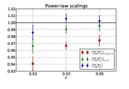
In Fig. (4.3) we plot the relativistic correlation function appearing in Eq. (2.1), , compensated for the expected scaling , with a linear vertical scale to help distinguish different power laws. We also plot the incompressible limit of that correlation function, obtained by setting (herein “the incompressible correlation”), as well as a non-relativistic but compressible version obtained by setting only (herein “the compressible correlation”). The former is equivalent to known results from incompressible Navier-Stokes turbulence (see Sec. (2.1.1)), while the latter can be obtained from the left-hand side of Eq. (2.1) using the non-relativistic perfect fluid energy-momentum tensor, which is just the relativistic one with . We use these comparisons to separately gauge the degree to which compressive and relativistic effects are important. In addition, we also include the predictions for each case, in matching colour, obtained from Eq. (2.1) and evaluations at and thereof. Error bars correspond to the statistical uncertainty .

For ease of comparison across cases, each plot has the same vertical axis range. As it is clear from the figure, we observe a progressive degradation of the scaling of the incompressible and compressible correlation functions as dissipation is weakened (and thus Mach number grows), while the relativistic one predicted in [2] outperforms. This is shown quantitatively in Fig. (4.4), where we display power law fits performed over the shaded interval of Fig. (4.3). The shaded interval is the same across all cases in order to make a fair comparison, and is chosen to capture the power law observed in the case (which has the narrowest scaling range). As dissipation is weakened, a monotonic shallowing of the best-fit power law is observed for both the incompressible and compressible correlation functions. This trend is more significant for the incompressible correlation function. The absolute performance of the relativistic correlation function is superior to the compressible and incompressible correlation functions across all cases, and its relative performance improves as dissipation is decreased (i.e. differences in best-fit power law become larger).
The relativistic correlation function, although exhibiting power-law scaling in all cases, nonetheless exhibits an increasing disagreement with the magnitude of the prediction in Eq. (2.1) (see Fig. (4.3)). In the most extreme case (, ), the overall magnitude is less than the prediction by . Our numerical ensemble of flows may be biased towards lower magnitudes, since runs with sufficiently large fluctuations from the random force can become numerically unstable and fail. As dissipation is weakened, this occurs more often. Thus, it is possible that the increasing disagreement of the magnitude of and is an artefact of this bias. A high-resolution shock-capturing implementation could determine whether this increasing disagreement is a real effect.
4.2 Direct-cascade simulation
To simulate the direct-cascade of a -dimensional conformal fluid, we instead use an external force with support only around , as described by Eq. (3.12). As in our inverse-cascade simulations, we use 4th-order numerical dissipation as in Sec. (3.2.3), with the choice . However, in contrast to our inverse-cascade simulations, here we use a large-scale dissipation mechanism known as 4th-order hypofriction, which takes the form of a term on the right-hand side of Eq. (3.10). We compute the inverse Laplacians spectrally, setting constant modes to zero. Such a term has power restricted to large scales, and terminates the brief inverse cascade from towards . We find the value to be adequate for preventing a build-up of energy (and eventual condensation) at large scales. An energy condensate would be characterized by continued energy growth and the emergence of two dominant vorticies of opposing parity superposed on a noisy flow (see eg. [53]). Statistical quantities are averaged over the shaded interval of time indicated in Fig. (4.5) (Left), which consists of snapshots separated by . The interval is chosen to maximize the number of snapshots available (to minimize statistical fluctuations), while remaining in a regime that roughly resembles a steady-state. Note that the measured correlations are not significantly affected if the temporal average begins slightly earlier or later. The average time step over this interval is , where is also averaged over the shaded interval. The injection rate of is measured initially to be . For reference, the characteristic time as per is , where we take since the maximum of the energy spectrum occurs at . The rms Mach number over the shaded interval is , once again indicating the weakly compressible regime.

In Fig. (4.5) (Left), we display the average Newtonian specific kinetic energy of the fluid as a function of time. As mentioned, we average various quantities over the shaded interval of time. The energy is beginning to plateau over this interval, however it continues to grow slowly. If evolved longer, the compressive component of the velocity begins to dominate over the curl-free part. To study such a regime more accurately, a Riemann solver would be desirable in order to more faithfully capture the dominant shockwave phenomena. Since we are instead using artificial high-order numerical dissipation, we choose to restrict our analysis to earlier times, when the compressive component of the velocity field is still subdominant ( of the total energy at a given scale - see Fig. (4.6) (Left)). Our high-order dissipation also results in large bottleneck effects at later times, which contaminate a rather large portion of the inertial range.
In Fig. (4.5) (Centre and Right), we display the probability distributions of the energy density (Centre, blue, solid) and Mach number (Right, blue, solid). For comparison, in both cases we also plot Gaussian distributions (black, dashed) with average and standard deviation matched to the data. Similar to the inverse-cascade simulations, the Gaussian provides a good fit to the Mach number pdf (although with weaker hints of a non-Gaussian tail in this case), whereas the energy density pdf exhibits a stronger, exponential tail towards smaller values.
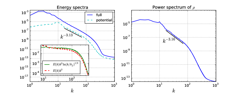
In Fig. (4.6) we display the power spectra of the velocity (Left) and energy density (Right). The full energy spectrum of the flow (blue, solid), together with the energy spectrum of the compressive, curl-free, potential part of the velocity (cyan, dashed). The latter is seen to be subdominant by a factor of over the range , which qualitatively corresponds to the direct-cascade interial range. The potential spectrum is fit by a power law over this range, while for the full spectrum we observe scaling with the multiplicative logarithmic correction . The inset shows the full spectrum compensated by with and without the logarithmic correction, with the presence of the logarithmic correction being favoured (flatter curve). In the literature, the presence of this correction seems to depend on several factors, including the length of time over which the average is taken, and the presence of large-scale dissipation [44, 54, 45, 55].
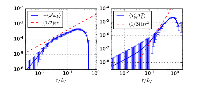
In Fig. (4.7), we display the two measured correlation functions for which we have predictions in the direct cascade (Eqs. (2.8) and (2.17)). Errors again correspond to the statistical uncertainty . We find reasonable agreement in the case of Eq. (2.8) (Left), and less so in the case of Eq. (2.17) (Right). The measured power laws are (Left) and , as compared to the predictions of and , respectively. However, we note that the non-trivial factors of (Left) and (Right) yield marked agreement in magnitude. We suspect that by decreasing contamination from our modified large- and small-scale dissipation mechanisms, agreement with our predictions would improve, since in our inverse-cascade simulations we found that removing large-scale dissipation altogether improved agreement with our predictions significantly. We also note that the statistical uncertainty at short length scales is large enough that the sign of the correlation functions is uncertain there. We estimate the quantity by its incompressible limit , with a further substitution of in place of (which improves agreement slightly). This estimate is justified by the fact that the correlation functions we measure do not differ significantly from their incompressible counterparts (i.e. setting ) in this regime.
Chapter 5 Discussion & Conclusions
As mentioned in Sec. (4.1), we observed that our energy spectra approach a scaling in the inverse-cascade range. We point out that it was observed in [51] that the incompressible case exhibits the same scaling provided large-scale friction is absent and the direct cascade is sufficiently resolved (, where we define ). It thus becomes a prescient question whether a sufficiently resolved direct cascade in the conformal fluid case will yield the same result. To answer this, we perform an ensemble of simulations with and , with a forcing profile given by Eq. (3.12). The resulting energy spectrum is displayed in Fig. (5.1), with the inset displaying the same spectrum compensated by either or . After filtering out the modes (i.e. all modes less than the maximum of the spectrum), the rms Mach number for this flow is . We perform this filtering so as to have a more fair comparison of rms Mach number with our inverse-cascade simulations in Sec. (4.1), which we remind were , , and . As evident from Fig. (5.1), the spectrum clearly favours a description in the inverse-cascade range, and not the Kolmogorov/Kraichnan description. The best-fit power law over the range yields .
Interestingly, we note in passing that this scaling of the energy spectrum would change the result of the purported calculation of the fractal dimension of a turbulent -dimensional AdS-black brane presented in [56] to (rather than ). An analysis of this will be the central topic in Part (IB).
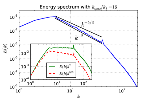
We also point out that, despite the narrow inverse-cascade range, we nonetheless observe a similarly narrow power law scaling in the same correlation functions analyzed in Sec. (4.1) (not shown). This suggests that the scaling relation Eq. (2.1) continues to hold with a more resolved direct-cascade range.
In Sec. (4.2), we observed hints of the predicted scaling of the correlation functions displayed in Fig. (4.7). By instead simulating an incompressible fluid (as per Sec. (3.2)), for which shockwave phenomena are not present, we can measure the incompressible limits of Eqs. (2.14) and (2.18) with greater statistical significance. Conformal fluids have been shown to possess a scaling limit to an incompressible Navier-Stokes fluid [57, 58]. We present the results of our simulation in Fig. (5.2) (Right). The enstrophy injection rate is set a priori to . We use 4th-order hypofriction and hyperviscosity , with and . The forcing profile is given by
| (5.1) |
and the injection scale is set to . The average specific kinetic energy is plotted as a function of time in Fig. (5.2) (Left), with the averaging interval shaded gray. The energy spectrum compensated by and is displayed in Fig. (5.2) (Centre), with the shaded envelopes indicating the statistical uncertainty . The logarithmic correction is clearly favoured. In Fig. (5.2) (Right), we plot the correlation functions and , together with their respective predictions in the direct cascade and . The agreement is very much improved over Fig. (4.7), which suggests that despite the low Mach number in our direct cascade simulation of the conformal fluid, that situation is nonetheless quite different from the incompressible case (at least insofar as the numerical challenges are greater in the former case, eg. small scales being contaminated by bottleneck effects).

Finally, at the beginning of this part in Fig. (IA) we display snapshots of the vorticity from several of our simulations. By doing so, we intend to provide intuition as to how the inverse and direct cascades appear in real space. In particular, the stretching and mixing of vorticity isolines characteristic of the direct-cascade range are readily identified as ‘turbulence’ qualitatively, where coherent features are seen over a variety of scales (see Fig. (IA) (Bottom Left) and (Bottom Right)). By contrast, the inverse-cascade range has a much noisier appearance, as in Fig. (IA) (Top Left). We have not observed an explicit acknowledgement of this qualitative fact in the literature, since numerical studies of the inverse-cascade range seldom include plots of the vorticity (eg. [1]). Unless the direct-cascade range is resolved, the turbulent flow qualitatively appears as random noise – but even if it is resolved, a clear hierarchy of scales is not apparent in the inverse-cascade range. In Fig. (IA) (Top Right) we show a mixed case with the forcing acting at an intermediate scale . This case is a simulation targeting the inverse-cascade range, but the direct-cascade range is just beginning to be resolved as well. Consequently, vorticity isoline mixing is beginning to be apparent, superposed on top of a more noisy structure.
Part IB Fractal dimension of turbulent black holes
Executive summary
The possibility of turbulent ringing of black holes has spurred recent interest and investigations. One question is how can we characterize their states, and [56] proposed using the concept of fractal dimension. We present numerical measurements of the fractal dimension of a turbulent asymptotically anti-deSitter black brane reconstructed from simulated boundary fluid data at the perfect fluid order using the fluid-gravity duality. We argue that the boundary fluid energy spectrum scaling as is a more natural setting for the fluid-gravity duality than the Kraichnan-Kolmogorov scaling of , but we obtain fractal dimensions for spatial sections of the horizon in both cases: and , respectively. These results are consistent with the upper bound of , thereby resolving the tension with the recent claim in [56] that . We offer a critical examination of the calculation which led to their result, and show that their proposed definition of fractal dimension performs poorly as a fractal dimension estimator on -dimensional curves with known fractal dimension. Finally, we describe how to define and in principle calculate the fractal dimension of spatial sections of the horizon in a covariant manner, and we speculate on assigning a ‘bootstrapped’ value of fractal dimension to the entire horizon when it is in a statistically quasi-steady turbulent state.
![[Uncaptioned image]](/html/1810.04594/assets/surfcontour_matchedcc.png)
Figure IB: Snapshot of a reconstructed black brane horizon from boundary fluid data.
Chapter 6 Introduction
In a certain regime, the existence of turbulence in the gravitational field was recently demonstrated in numerical simulations of a perturbed black brane in asymptotically anti-deSitter (AAdS) spacetime in [56]. Such behavior was expected on the basis of the work of [13] and the fluid-gravity duality, which gives an approximate dual description of the bulk geometry in terms of a conformal fluid living on the conformal boundary of the spacetime (see eg. [11, 59, 60], or [61] for a review and further references). This duality has opened the door to cross-pollination between the fields of gravity and fluid dynamics (eg. [62, 12, 13, 25, 63, 64, 56, 65, 66, 2, 67]), and even resulting in insights with potential relevance to gravitational wave astrophysics [68].
Interestingly, in [56] it was argued that a -dimensional AAdS-black brane spacetime in a turbulent quasi-steady state has an event horizon with fractal dimension . Although the intersection of the horizon with a spacelike slice has dimension , in a turbulent state one expects a bumpy horizon exhibiting approximate self-similarity over some range of scales, and therefore a fractal dimension in the range . Since the result of [56] lies above this range, it is in tension with this basic expectation. Indeed, since is Riemannian and connected, it can be regarded as a metric space where its distance function is defined as the infimum of lengths of paths connecting any two points. Therefore, since is embedded in it, its fractal dimension cannot exceed the dimension of [69].
In this work we begin in Chapter (7) with a review of the relevant calculation in [56], then in Sec. (7.1) we provide a critical examination. We argue that their calculation does not use their proposed definition of fractal dimension, and so the fact that their result exceeds the upper bound does not necessarily invalidate their definition. Nonetheless, in Sec. (7.1.1) we argue using well-understood test cases of statistically self-similar 1-dimensional curves embedded in the Euclidean plane that their proposed definition of fractal dimension is not reliable as a fractal dimension estimator. Next, in Chapter (8) we present an alternative numerical calculation of the fractal dimension of a turbulent black brane using simulated data of the dual turbulent fluid and the fluid-gravity duality at lowest (perfect fluid) order. We do so over the inverse-cascade range of a weakly-compressible conformal fluid with two sets of data corresponding Kraichnan-Kolmogorov scaling of the energy spectrum as well as the scaling which emerges as the direct-cascade becomes well-resolved (and in the absence of large-scale friction) [51, 67]. We obtain fractal dimensions of and for each case, respectively, thus removing the aforementioned tension concerning the claim that . Lastly, in Sec. (8.1) we describe what would be required to define, and in principle compute, the fractal dimension covariantly.
Chapter 7 Background
In this section we briefly review the argument presented in [56], specializing to the case of a -dimensional bulk spacetime. Further details can be found in that work.
In [56] it is proposed that the fractal dimension of the horizon be defined via the scaling of the horizon area course-grained on a scale . Writing the course-grained area as a Riemann sum of the intrinsic area elements , with and the intrinsic metric determinant evaluated at the point , one extracts the purported fractal dimension from the scaling . One can immediately see that this definition has some of the expected behaviour: i) if the intrinsic metric determinant is constant over the surface, then the course-grained area does not depend on so we must have (a smooth surface), ii) as the surface becomes rough (), the area grows faster as decreases (and indeed becomes infinite as ).
The calculation of the fractal dimension begins by considering the congruence of null geodesics generating the horizon. This is described by the Raychaudhuri equation in vacuum, which governs the evolution of the horizon area element ,
| (7.1) |
where is the null normal to the horizon, is a Lie derivative along , is the non-affinity of measured by the right-hand side of the geodesic equation , and is the shear. The regime of validity of the fluid-gravity duality is that of slowly-varying fields, so one expects the higher-order derivative terms and to be subleading with respect to both the right-hand side and the lower-order derivative term . Dropping those higher-order terms and integrating over the spatial section of the horizon yields an expression for the time rate of change of the horizon area ,
| (7.2) |
where is the isotropic power spectrum of the ‘rescaled’ shear , and the last equality follows from the Plancherel theorem. In [56] it was observed in full numerical simulations of a (3+1)-dimensional turbulent AAdS-black brane spacetime that , at least in the regime of the simulations, where is the isotropic velocity power spectrum of the boundary fluid. By assuming Kraichnan-Kolmogorov scaling over the inverse-cascade range, one has there. By inserting a large wavenumber cutoff in the wavenumber integral in Eq. (7.2) one finds for in a sufficiently wide inverse-cascade range. Matching this to the scaling finally yields .
One may object that the scaling is to be applied to , not . However, in the quasi-steady state of a turbulent fluid forced at scale with inertial range scaling extending to a large scale , the spectrum is well-approximated by piecewise power laws with the inertial range portion over unchanging except that decreases with time (see eg. [70]). I.e. the inertial range becomes larger with time, but the spectrum over that range does not change. Plugging such a piece-wise power-law into the right-hand side of Eq. (7.2) with UV cutoff allows one to perform both the wavenumber and time integration explicitly. Thus the piecewise power-law model of relevant to turbulent flows in quasi-steady state implies that and scale in the same way with the UV cutoff , for sufficiently large. In the following section, we identify other possible sources of problems with the calculation.
7.1 Critical examination of [56]
We begin by noting what it means in position space to insert the small-scale cutoff in the wavenumber integral in Eq. (7.2). In order to do this we must write explicitly [56]:
| (7.3) |
where is the Fourier transform of the rescaled shear, . Eq. (7.3) can be rewritten as
| (7.4) | |||||
Therefore the wavenumber integral in Eq. (7.2) is just the integral of over all of Fourier space. Furthermore, note that integrating over is the same as multiplying by a step function kernel and then integrating over , and writing it in this way allows us to see the meaning of the cutoff in position space as follows:
| (7.5) | |||||
where is the Bessel function of the first kind, and we have defined as a spatial coarse-graining operation at scale (in this case with an isotropic kernel ).
We thus arrive at our first concern: the relationship between Eq. (7.5) and the proposed coarse-graining is unclear. The latter is a Riemann sum, which if applied to the Raychaudhuri Eq. (7.2) would yield . The summand could be viewed as a coarse-graining of both factors of the rescaled shear , whereas in Eq. (7.5) only one factor of is coarse-grained. Thus, even if the scaling correctly captures the fractal dimension , it is unclear whether the calculation performed in [56] uses it.
7.1.1 Comparing methods on -dimensional test cases
Next, we argue that the Riemann sum approach is a poor fractal dimension estimator. We consider the 1-dimensional version of this, , applied to three different noise curves in the Euclidean plane whose fractal dimensions are known. We refer to this proposed method of determining the fractal dimension of a curve as the ‘intrinsic metric method’. Despite a strong resemblance, the intrinsic metric method of approximating the length of the curve is distinct from the ‘compass’ or ‘ruler’ method appearing in the pioneering study of coastline lengths [71], since the former involves approximating the curve by its tangents at the points , which are line segments of unequal length and whose end points do not necessarily lie on the curve. Each curve is defined by a function , and therefore has an intrinsic metric induced by the Euclidean metric of its embedding space whose determinant is . Thus we can compute coarse-grained versions of the length of the curve as and then compare with the expected scaling . For comparison, we estimate the fractal dimension of the same curves using the madogram method described in [72]. The madogram is defined as , where denotes a spatial average. The madogram is expected to scale as .
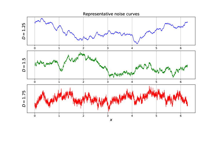
Fig. (7.1) shows a comparison between the intrinsic metric and madogram methods for estimating the fractal dimension of three noise curves with (blue), (green), (red). Such noise curves have power spectra scaling as for , , , respectively. For the range a topologically -dimensional surface has a fractal dimension related to the spectral exponent by the approximate relation [73]. For the surface is sufficiently smooth that the fractal dimension equals its topological dimension, , whereas for it saturates to . In Fig. (7.2) we display representative curves with fractal dimensions (blue, Top), (green, Middle), and (red, Bottom).
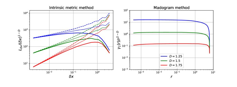
An ensemble of size is generated for each noise curve, and the estimators and are computed for each member and then averaged over the ensemble. In the intrinsic metric method, it is insufficient to attempt a single set of sampling locations for a given . Instead, we start with the zeroth set of sampling locations , but also try additional sets related to the first by a translation for the th set, for a total of sets. This results in length estimates for each , and we consider taking the minimum, maximum, or median length estimates, shown in Fig. (7.1) (Left) in thick solid, thin solid, and dashed curves, respectively. Such “shifts” are an essential part of many fractal dimension estimating algorithms. Box-counting, for example, requires finding the minimum number of boxes that cover the object, so many shifts of the box grid must be tried in order to obtain an accurate estimate. A priori we do not know whether to take the minimum, maximum, or median estimate of the length . Different methods for estimating the fractal dimension have different conventions, for example the ‘compass’ or ‘ruler’ dimension [71] takes the maximum length, ‘box-counting’ takes the minimum number of boxes [74], and ’line transect variogram’ methods applied to a surface take the median result from the transects [72]. However, as Fig. (7.1) (Left) shows, none of the three possibilities yield the expected scaling over any discernable range of . We note that taking the average or the median yields nearly identical curves (thin solid).
Chapter 8 Results
Using the numerical code described in [67] and Part (IA), we evolve a -dimensional conformal perfect fluid with equation of state on a -periodic domain with points. The energy momentum tensor of the fluid is , with and the Lorentz factor. The fluid is evolved from rest , , and turbulence is induced and sustained by a random external force with homogeneous, isotropic, Gaussian white-noise-in-time statistics. The external force has support in a narrow band of wavenumbers around . Further details can be found in [67].
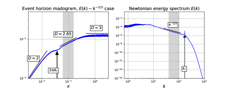
An inverse-cascade range develops, and since we do not implement any large-scale energy sinks, the resulting flow is referred to as being in a quasi-steady state [51]. For two separate cases with and , we generate an ensemble of flows and perform analysis on snapshots prior to the energy piling up at the scale of the box. As displayed in Fig. (8.1) (Right), the case yields an isotropic Newtonian specific kinetic energy spectrum , as found in [51] in the incompressible case and confirmed in [67] for a conformal fluid in the weakly-compressible regime.111It was found in [51] that the spectrum steepens to when , where and is the number of points on the grid. In our simulations this would correspond to , but in their case regular 2nd-order viscosity was used, whereas we use 4th-order dissipation. Thus, we are able to achieve the spectrum with a much larger because our dissipation operates at larger wavenumbers. The scaling is associated with both a well-resolved direct cascade and an absence of large-scale friction. Since the regime of validity of the fluid-gravity duality is that of an arbitrarily high Reynolds number and no large-scale friction, we argue that this spectrum corresponds to the natural setting for the dual spacetime. However, for comparison we also consider the case, where the force is active deeper into the dissipation range, and which yields the traditional Kraichnan-Kolmogorov scaling , as displayed in Fig. (8.2).
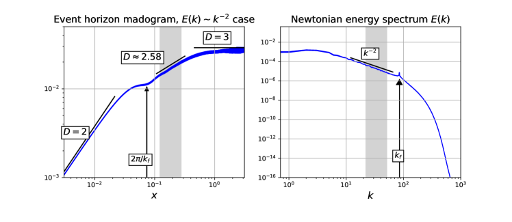
We applied the madogram method to - and -transects of the event horizon. The fractal dimension of the horizon is then obtained by extracting from the median madogram of each topologically -dimensional transect, and then writing . Such a prescription is valid for surfaces exhibiting statistical self-similarity, and its performance was evaluated extensively in [72]. In Figs. (8.1) and (8.2) (Left) we display the median madogram over all transects of the horizon (herein referred to as the ‘event horizon madogram’), as applied to the radial coordinate position of the event horizon, , for the perturbed boosted AAdS-black brane metric at perfect fluid order,
| (8.1) | |||||
where the indices run over the ‘boundary’ directions only, is the AdS length scale (which we set to 1), is the boost -velocity, and is the -dimensional Minkowski metric. For the -dimensional boundary conformal fluid, . The perturbations are imagined to be slowly-varying with respect to the boundary directions, which will solve Einstein’s equations with arbitrary accuracy in the perfect fluid limit if and evolve according to conformal hydrodynamics on the boundary. Error estimates have been obtained for solutions constructed from particular boundary fluid data in [56] via direct comparison with full GR simulations, showing agreement at the level (see also [65] for error estimates which do not use full GR simulations).
Fig. (8.1) shows the case with and Fig. (8.2) shows the case with . The thickness of each plot indicates the statistical uncertainty associated with the ensembles. At small scales , the horizons have fractal dimension , which agrees with their topological dimension. This is expected since rough structure does not persist down to arbitrarily small scales. For a range of scales greater than the forcing scale , power-law behavior is observed in both cases. A least-squares power-law fit over the grey shaded intervals yield a fractal dimension of and for the cases and , respectively, with uncertainties indicated. The corresponding fitting interval in Fourier space is indicated on the plots of the energy spectra (Right). The madograms saturate at at large scales, beyond the inertial range scale, which is due to the flow resembling white noise at those scales (i.e. constant).
8.1 Covariant construction of fractal dimension
Many methods exist for calculating the fractal dimension of a set embedded in an ambient metric space , where is a distance function which is symmetric and satisfies and the triangle inequality . See eg. [72] for a comparison of many fractal dimension estimator algorithms when the metric space is Euclidean, or [75, 74] for strictly mathematically equivalent definitions. For illustrative purposes, we will focus on the box-counting method in this section, where one defines to be the minimum number of boxes of size in the embedding space required to completely cover the set , and then computes the fractal dimension as . The box-counting method is known to be diffeomorphism-invariant but not homeomorphism-invariant [76] in the strict limit. The covering need not use boxes; indeed, any sets of diameter yield the same result [69].
In practical applications one does not take the limit, but instead fits a power-law to over some finite range . If the covering sets are not constructed covariantly, then any such fitting over would be subject to coordinate ambiguity, since the set in question could be made to appear smooth over the scale via a judicious choice of coordinates. In the example of a Brownian noise curve with , described by in Cartesian coordinates in Euclidean space, one could make the coordinate transformation (, ), where is with all modes outside the range of scales filtered out. Counting coordinate boxes over the scales would then give the incorrect result . Thus, it is important to construct the covering sets in a diffeomorphism-invariant way when performing a fit over the range of scales .
When defining fractal dimension over a Riemannian manifold, one natural covariant choice of covering sets are geodesic balls , constructed by taking the union of all geodesics of length emanating from the point . The event horizon on the slice is embedded isometrically both in and , where is the full spacetime metric and is the induced metric on . Since geodesic paths in need not be geodesic in , one is faced with the choice of whether to cover with geodesic balls in or in 222Since has a Lorentzian metric signature, a geodesic ball as defined above would contain the entire light cone of the central point since the length along null paths is zero. Thus, in this case we can instead define the geodesic ball as the union of only those spacelike geodesic paths of length emanating from which intersect at a point .. But note that the slice itself could be deformed at points off of to yield different geodesic paths while sharing the point set . Thus, constructing the geodesic balls in would yield a fractal dimension which is not solely a property of , but rather dependent on the arbitrary choice of slicing away from . For this reason, we advocate using geodesic balls constructed in the full spacetime (with a suitable redefinition - see footnote2).
Computed in this way, a geodesic ball-counting procedure over a range of scales would yield a fully covariant estimate of the fractal dimension of any given spatial section of the event horizon. Furthermore, recall that our ensembles of event horizons considered in Chapter (8) yield roughly the same fractal dimension. It is often observed that cross-sections of -dimensional fractals or statistically self-similar objects themselves have a fractal dimension of (see eg. [77] for geological examples). Given our measurement of in Chapter (8) for the case, this suggests that in a quasi-steady turbulent state the entire horizon can be assigned a fractal dimension of (or for the Kraichnan-Kolmogorov case ). However, the mathemetical meaning of this is not clear since is a null hypersurface embedded in a Lorentzian manifold , so there is difficulty in defining the diameter of covering sets in a covariant way.
Numerically implementing the procedure described in this section would be expensive, since one would have to integrate a large number of geodesics from a given point to construct a geodesic ball, do so for many geodesic balls to find a covering, and do this for many possible coverings to find the minimal one. In the current work we have not followed a covariant procedure like this. Many others have not either (eg. [78, 79, 80, 81, 82]), some opting instead to point out the diffeomorphism-invariance of box-counting in the limit while only fitting over a finite range . It would be interesting to see how much these results change when done covariantly.
Alternatively, it is plausible that the fractal dimension will not depend sensitively on the embedding space if, in a region around the surface, one has well-separated scales over which the surface and the embedding space vary. If this is true, once could obtain an approximate covariant result by embedding the surface isometrically in Euclidean space, and then applying a standard fractal dimension estimator. We attempted to embed the turbulent horizon isometrically in , without success. Indeed, the existence of such a (global) embedding is only guaranteed if the Gaussian curvature is positive over the entire surface, and may or may not exist otherwise. It has been observed [83] that even a sufficiently rapidly-rotating Kerr black hole horizon does not have a global embedding in , since the Gaussian curvature becomes negative at the poles. We have computed the Gaussian curvature using our fluid data from Chapter (8), and observed that it changes sign over the domain as rapidly as the external force. Thus, we believe it is highly unlikely that there exists a global embedding into for arbitrary turbulent horizons in the regime of the fluid-gravity duality, although Euclidean embeddings are guaranteed to exist in sufficiently high dimensions.
Chapter 9 Conclusions
In this work we provided a critical examination of the calculation in [56] which led to the claim that topologically -dimensional turbulent AAdS-black brane horizons embedded in a -dimensional Riemannian space have a fractal dimension , exceeding the upper bound of . We offered an alternative numerical computation of when , and discussed issues surrounding the covariance of that quantity.
In particular, we argued using well-understood test cases of -dimensional noise curves that the proposed definition of fractal dimension in [56], , when specialized to topologically -dimensional objects, performs poorly as a fractal dimension estimator. We emphasize that this is not a proof that the definition fails in the strict limit for genuine fractals, but since the proposed application is on statistically self-similar surfaces which do not exhibit rough structure down to arbitrarily small scales, the performance of this proposal as a fractal dimension estimator is relevant. Furthermore, we argued that the calculation in [56] may not be using their proposed definition at all (so their result of alone does not necessarily invalidate their proposed definition, hence our separate evaluation of the definition on noise curves of known fractal dimension).
Using simulated turbulent conformal fluid flows in the quasi-steady state regime, we constructed snapshots of the turbulent event horizon using the fluid-gravity duality at perfect fluid order. By applying a line transect madogram method [72] to the event horizon surface in boosted ingoing Finkelstein coordinates, we obtained a fractal dimension for spatial sections of the horizon of and for the cases with the boundary spectrum and , respectively. We argued that the former scaling, , is a more natural setting for the fluid-gravity duality since it corresponds to the regime of infinite Reynolds number without large-scale dissipation of energy [51, 67].
We also speculated that in the quasi-steady state regime, since the fractal dimension will statistically not depend on the particular time at which a spatial section of the horizon is considered, that the entire horizon could be assigned a ‘bootstrapped’ fractal dimension of , although the strict mathematical meaning of this is not clear. Furthermore, we have not shown that is invariant with respect to deformations of the spatial section of the horizon (when computed over an ensemble of horizons), since we have only considered constant time slices in the ingoing Finkelstein coordinate.
Part II Post-Newtonian approach to black hole-fluid systems
Executive summary
Many interesting astrophysical systems have a combination of very long characteristic times and important general relativistic effects. For a subset of these systems, propagating gravitational degrees of freedom are of subleading importance, and thus allow for approximate descriptions. In this part, we present our progress in implementing and testing a post-Newtonian gravity-hydrodynamics (PNGhydro) code in spherical symmetry. The post-Newtonian (PN) formalism was presented in [84] and is capable of describing the interaction between a black hole and a fluid up to 2.5 PN order. The equations governing the gravitational potentials are all elliptic, owing to the use of the Poisson gauge. This eliminates propagating degrees of freedom from the problem, and thus would be advantageous to implement in a numerical code for the study of systems requiring very long integration times, eg. tidal disruption events. We will also present a general relativistic hydrodynamics (GR fluid) code in spherical symmetry which we developed to provide a benchmark against which to measure the accuracy of the PNGhydro code. Since this is a proof-of-principle, we make no attempt to lower the computational cost of the PNGhydro code with respect to the GR fluid one.
![[Uncaptioned image]](/html/1810.04594/assets/x15.png)
Figure II: Preview of the numerical evolution of a fluid pulse, injected into the spacetime of a vacuum black hole of mass via the outer boundary.
Chapter 10 Introduction
Many astrophysical systems of interest involve relativistic gravitating fluids in a regime where the propagating degrees of freedom of the gravitational field are of secondary importance compared to the fluid physics and conservative gravitational effects. Among these are core-collapse supernovae (CCSNe) in the early post-bounce regime, where gravitational wave damping of modes excited by core bounce is outdone by other effects [85, 86], and tidal disruption of stars with low compactness by black holes (eg. [87, 88, 89]). Even in modern investigations, for the sake of finding cost reductions the former is often treated in Newtonian gravity [90, 91, 92] or with phenomenological general relativistic corrections [93, 94]. Tidal disruption events (TDEs) have the added complication of a black hole, which brings relativistic effects such as an innermost stable circular orbit (ISCO) and spin coupling. “Pseudo-Newtonian” treatments of black holes have been employed via phenomenological potentials [95, 96, 97, 98], not restricted to the tidal disruption context, or test-fluid evolutions on non-reactive black hole backgrounds with Newtonian self-gravity of the star [99].
In the TDE case, there is a large separation of scale between the characteristic speeds of gravity and hydrodynamics: the speed of light and the speed of sound, respectively. Degrees of freedom propagating at the speed of light require smaller time steps to resolve, and if such degrees of freedom are of subleading importance (as they typically are when the star has low compactness), then it is wasteful to resolve them. This problem is exacerbated by the fact that the orbital dynamics in a TDE occur over a large spatial scale, and especially by the fact that long integration times are required. The former can be addressed with mesh refinement techniques, but not the latter. For these reasons, a formalism which captures essential features of gravity, short of propagating effects, is desirable. This can be achieved through a post-Newtonian (PN) approximation.
Note that other approaches to simulating TDEs exist which do not use pseudo- or post-Newtonian treatments of gravity. For example, in [100, 101] the star is followed in Fermi normal coordinates on a fixed black hole background, allowing the tidal effects to be computed at various orders. Another strategy used in [102, 103] is to subtract the truncation error due to the dominant black hole background (whose analytic solution is known). While these approaches capture hydrodynamics and gravity, they lack the sophisticated microphysics of the pseudo-Newtonian codes which allow the computation of multi-wavelength electromagnetic emission and nuclear reactions (eg. [104, 105, 106]).
A PN formalism was presented in [107] which gives the dynamics in terms of Poisson equations. The purpose of this was for Newtonian gravity codes to easily include relativistic corrections, since they already solve Poisson equations. This formalism did not include black holes, and subsequent numerical implementations used massive point particles as stand-ins for black holes [108, 109] (see [110] for the inclusion of some spin effects). Producing sufficiently massive stars to represent neutron stars has been reported to be difficult in this formalism [84].
A similar PN formalism was written down to higher order in [84], and it can describe a fluid-black hole system. The mass-radius curve of cold equilibrium neutron stars represented by a polystopic perfect fluid with , was reproduced fairly well down to km radius in isotropic coordinates. Furthermore, the ISCO radius, when measured in a gauge-invariant manner as , is tracked well for spin parameters , whereas the pseudo-Newtonian potential of [95] does not depend on at all. In this formalism, the post-Newtonian potentials due to the Kerr black hole are given analytically. Owing to the use of the Poisson gauge, the hydrodynamic contribution to the potentials is determined by a set of elliptic partial differential equations, and thus has no propagation speeds. We reiterate that if implemented in a numerical code, this formalism would therefore allow the propagating degrees of freedom of the gravitational field to be ignored. Larger time steps would therefore be possible, reducing the cost of the long integrations required in tidal disruption systems. Furthermore the relativistic effects would be faithfully captured to the prescribed order, and the regime of validity of any integration would be known a priori. This is contrasted with pseudo-Newtonian approaches where some of the physics is captured but not others, and errors are not under control due to the lack of a systematic expansion.
In this part, we present our progress towards implementing a proof-of-principle of the formalism in [84] in a spherically-symmetric gravity-hydrodynamics code. We also develop a general relativistic hydrodynamics code (GR fluid) as a benchmark against which to test the post-Newtonian gravity-hydrodynamics (PNGhydro) code. Spherical symmetry eliminates the radiative dynamics and renders a subset of the PN potentials unnecessary, so this is not a full demonstration of the formalism, but it is a logical first step.
This part is organized as follows.
In Chapter (11) we provide extensive background material and discussion of our methods. This includes a discussion of the fluid equations in curved spacetime in Secs. (11.1), (11.2), and (11.3). The formulation of Einstein’s equation we use and the derivation of constraint-preserving boundary conditions are discussed in Secs. (11.4) and (11.5), respectively. We provide an overview of the PN formalism of [107, 84] in Sec. (11.6).
In Chapter (12) we present details of our numerical implementation. This includes a review of aspects of computational fluid dynamics in Secs. (12.1), (12.2), and (12.3). In Sec. (12.4) we describe our method of injecting fluid matter into the domain through the outer boundary, which eliminates the need for a numerical initial data solver. We describe the current state of our PNGhydro implementation in Sec. (12.5).
Chapter (13) contains a variety of code validations, including “artificial analytic convergence tests” (13.1), evolutions of a stable TOV star (13.2), injection of gauge and fluid pulses into a black hole spacetime (13.3), (13.4), and an independent residual test of the PN solver (13.5).
Finally, we present preliminary results and conclusions in Chapter (14).
Chapter 11 Background and methods
11.1 3+1 Form of the Fluid Equations
In this section, we present the hydrodynamic equations on an arbitrary background geometry in coordinate-free 3+1 form. This is for mainly for an illustration of how to go from covariant expressions to coordinate-free 3+1 form, and we will be very verbose. Although one can obtain a coordinate representation from this form, like the Valencia formulation [111] we describe in Sec. (11.2) and use in our code implementation, in practice we bypass this step by introducing coordinates right away. One may therefore skip this section without loss of continuity.
In terms of the stress energy tensor , rest mass density , and fluid 4-velocity , we begin with the general covariant form of the equations,
| (11.1) | |||||
| (11.2) |
where Eqs. (11.1) and (11.2) express the covariant conservation of stress-energy and baryon number, respectively. We introduce to our spacetime a spacelike foliation described by the timelike unit normal vector field to the hypersurfaces , intrinsic metric of the hypersurfaces , and extrinsic curvature of the hypersurfaces . We have chosen the mostly positive signature and defined the acceleration of the fundamental observers as . The foliation and some related quantities (to be used explicitly in later sections) are depicted in Fig. (11.1)
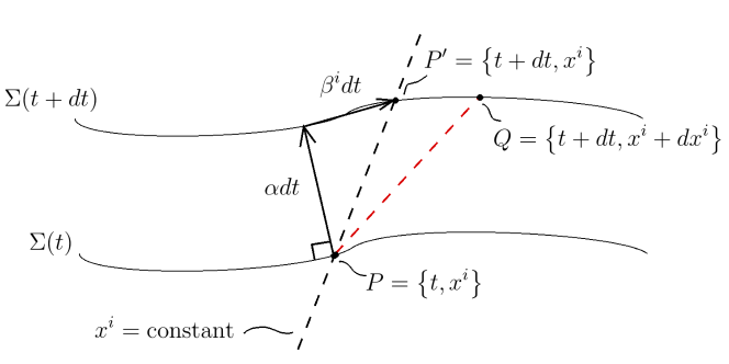
To obtain the 3+1 form of energy conservation, we must project Eq. (11.1) onto the direction as follows:
At this point let us define the energy density , the energy current , and the purely spatial projection of the stress-energy . We thus obtain
| (11.3) |
The first two terms include a full spacetime covariant derivative, which must be further decomposed as follows:
| (11.4) | |||||
Putting Eqs. (11.3) and (11.4) together, we obtain the final form of energy conservation,
| (11.5) |
Next, to obtain the 3+1 form of momentum conservation, we apply instead the projector to Eq. (11.1):
| (11.6) | |||||
Finally, we can also manipulate the scalar expression of baryon number conservation, Eq. (11.2), as follows:
Defining the Lorentz factor between the fundamental observers and the fluid velocity as and the spatial fluid velocity as , we go on to write
| (11.7) | |||||
This concludes the coordinate-free 3+1 decomposition of the hydrodynamic equations.
11.2 The Valencia formulation of hydrodynamics
We employ the Valencia formulation [111] of hydrodynamics in our numerical setup. This formulation is flux-conservative, and convenient for shock-capturing methods. We briefly describe the formulation here, following [112].
We will make use of the identity
| (11.8) |
as well as its generalizations to mixed rank-2 tensors,
| (11.9) |
and contravariant rank-2 tensors,
| (11.10) |
We assume a -dimensional split of spacetime, where is the lapse function, is the shift vector, and is the spatial metric whose determinant is related to the full spacetime metric via . Recall the Lorentz factor . With we have . The coordinate velocity of the fluid is related to its velocity in the frame of the fundamental (Eulerian) observers through the lapse and shift as . By applying Eq. (11.8) to local mass conservation and using the aforementioned relations, we obtain
| (11.11) | |||||
where we have defined the conservative variable .
Similarly for the spatial component of energy-momentum conservation, . First note that . Then using Eq. (11.9) and we can write
| (11.12) | |||||
where we have defined the conservative variable . Written in this way, this equation of motion has a source term coming from the spacetime curvature.
Lastly, the time component of the energy-momentum conservation we treat with indices up, , and some manipulation is required. First note that and . We prepare for the overall factors of by rewriting
Then, applying Eq. (11.10) to , we obtain
| (11.13) | |||||
where we have defined . It is advantageous to subtract Eq. (11.11) from Eq. (11.13) to obtain an equation of motion for instead, since the Newtonian limit of is [111] and thus will be numerically more accurate for non-relativistic flows. Doing so results in
| (11.14) |
We furthermore choose to absorb a portion of the spatial metric determinant into the definition of certain variables, resulting in densitized variables. With a spatial metric in spherical symmetry given by , the factor we absorb is . We densitize the primitive mass density , resulting in . This change propagates to and , via their definitions. Given an ideal fluid equation of state , this also results in and thus as well. For other equations of state not necessarily linear in , eg. polytropes , care must be taken to undensitize in a numerical code before using such a formula.
11.2.1 Specialization to spherical symmetry
In this section we specialize the system of hydrodynamic equations (11.11), (11.12), (11.14) to spherical symmetry. We will encounter some regularization issues at the origin, and will fix them with a clever rewriting of the equations.
In spherical symmetry the vector has only a radial component , so our densitized hydrodynamic variables are
| (11.15) | |||||
The equation of motion (11.11), (11.12), (11.14) become, respectively,
| (11.16) | |||||
| (11.17) | |||||
| (11.18) |
where the source terms and on the right-hand sides are given by
| (11.19) | |||||
| (11.20) | |||||
The first regularization issue concerns the derivative operators, which if evaluated naively at numerically would give an infinite result. We rewrite this operator as , which by the chain rule is equivalent.
The second regularization issue concerns the term in Eq. (11.19), which also presents a problem at the origin. The key fact to understand with a formally infinite term such as this is that it is merely a coordinate singularity. Thus, the mathematics should work out to eliminate the divergence, we just have to find the appropriate rewriting of the equation. We notice that a piece of the flux term on the left-hand side of Eq. (11.17) actually cancels the offending source term. Namely, we can rewrite Eq. (11.17) as
| (11.21) |
which eliminates the divergent source term on the right-hand side. This is called the flux-splitting method, since we have split the flux into two separate pieces in order to pull out the corresponding divergent term which appears in the source on the right-hand side.
11.3 Characteristic structure of hydrodynamics in curved spacetime
In this section we review the characteristic structure of hydrodynamics in general relativity, specialized to spherical symmetry and an ideal fluid equation of state , which yield significant simplifications. The characteristic structure of the system of Eqs. (11.11, 11.12, 11.14) in Sec. (11.2) were derived in the special relativistic case in [113], and then in the general relativistic case in [114]. We follow the latter reference here.
In spherical symmetry, the system of Eqs. (11.11, 11.12, 11.14) takes the form
| (11.22) |
whose principal part gives
| (11.23) |
The factor is a matrix containing the characteristic structure of the system. Its eigenvalues correspond to the characteristic speeds, and for an ideal fluid equation of state are given by
| (11.24) |
where is the sound speed, given in terms of the specific internal energy as . The eigenspeed corresponds to the material wave, whereas correspond to acoustic waves. Setting , , taking , and keeping lowest orders in yields the Newtonian expressions
| (11.25) |
A complete set of right-eigenvectors of corresponding to the eigenvalues in Eqs. (11.24) are
| (11.26) |
where the enthalpy is . The corresponding left-eigenvectors (i.e. the rows of the matrix ) are
| (11.27) |
The characteristic variables are obtained as follows. For clarity, first rewrite Eq. (11.23) as
| (11.28) |
where the subscripts denote partial differentiation, and the matrix . The matrix can be diagonalized so that , where and is the matrix whose columns are the right-eigenvectors of , . This gives
| (11.29) | |||||
In the last line we brought into the derivatives while ignoring the terms which would ordinarily compensate for this. Since this characteristic analysis assumes linearization on a background solution, those compensating terms are lower order (in the sense of characteristic analysis) because is built from the background solution and so no derivatives of the perturbation are present. This justifies ignoring the compensating terms when bringing into the derivatives.
We have decoupled the equations by transforming to the variables , known as the characteristic variables, and within this linear regime they propagate at the characteristic speeds given by Eq. (11.24). In our case of an ideal fluid, the characteristic variables are
| (11.30) |
11.4 Einstein-Christoffel formulation of general relativity
In this section we describe the Einstein-Christoffel formulation of general relativity [115], which we use in our simulations. This is a first-order formulation of general relativity, where the shift and densitized lapse are specified a priori and thus are treated as non-dynamical. After writing the general equations, we will specialize to spherical symmetry, largely following [116], and perfect fluid hydrodynamics. We use a -decomposition of spacetime, as described during the course of Secs. (11.1) and (11.2).
We begin with the Hamiltonian and momentum constraint equations, which follow from a full and partial projection of the Einstein equations
| (11.31) |
onto the normals to the foliation via contraction with and , respectively [112]:
| (11.32) | |||||
| (11.33) |
where and are the ADM energy density and current coming from matter sources, respectively. Observers moving orthogonally to the spacelike foliation will measure this energy density and current. The evolution equation for the extrinsic curvature of the foliation hypersurfaces is obtained via a full projection of Einstein’s equations (11.31) onto the hypersurfaces via contraction with :
| (11.34) | |||||
where is the spatial energy-momentum tensor and . The evolution of the intrinsic metric follows from the definition of the extrinsic curvature:
| (11.35) |
Specializing to spherical symmetry and perfect fluid hydrodynamics, we write
| (11.36) | |||||
| (11.37) |
where all fields depend on the coordinates only. Two auxiliary variables are used to reduce the system to first-order, which are
| (11.38) | |||||
| (11.39) |
The energy-momentum tensor of a perfect fluid reads , which gives the ADM matter sources as
| (11.40) | |||||
| (11.41) | |||||
| (11.42) |
The constraints Eqs. (11.32) and (11.33) become
| (11.43) | |||||
| (11.44) |
The definition of our auxiliary variables Eqs. (11.38) and (11.39) also constitute constraints, i.e.
| (11.45) | |||||
| (11.46) |
As mentioned earlier, the shift and the densitized lapse are taken to be specified a priori. The evolution equations for the intrinsic metric become
| (11.47) | |||||
| (11.48) |
The evolution equations for the extrinsic curvature become
| (11.49) | |||||
| (11.50) |
Our auxiliary variables and also have evolution equations, given as
| (11.51) | |||||
| (11.52) |
11.5 Constraint-preserving boundary conditions
The freedom in choosing boundary conditions is encapsulated in the choice of ingoing characteristic modes. However, only a subset of the possible choices will also satisfy the constraints of the theory. Without care, the boundary treatment can therefore introduce constraint violating dynamics onto the computational grid, which degrade the quality of the numerical solution. In the general simulation conditions of full dimensionality and arbitrary gauge choices, the negative impact of constraint-violating boundary conditions can be lessened through a variety of means. This includes pushing the boundary farther out into the asymptotically flat regime, which is feasible on a cost basis with mesh refinement techniques, but is still wasteful. Implementing constraint-preserving boundary conditions in such general situations can be quite complex, but in spherical symmetry it is more straightforward. We implement this in our GR fluid code, and describe how to do so in this section.
We can restrict our choice of boundary conditions to the narrower set of the constraint-preserving ones via an analysis of the characteristics of the system of constraints themselves. The constraints may possess ingoing characteristic modes, and by setting them to zero we can obtain the restrictions that we seek. In this section, we describe this procedure for the Einstein-Christoffel formulation of general relativity in spherical symmetry, following [116].
We begin by taking time derivatives of the constraints Eqs. (11.44) and (11.46). On the right-hand sides we can trade time derivatives for space derivatives using the equations of motion of the main variables, Eqs. (11.48), (11.50), and (11.52). Then one rewrites the space derivatives of the main variables in terms of the constraints themselves, and their space derivatives. Since we are only interested in the characteristics of the system, we can keep the principal parts and discard lower-order terms throughout this procedure, which greatly simplifies the calculation. The result, up to the principal part, is
| (11.53) | |||||
| (11.54) | |||||
| (11.55) | |||||
| (11.56) |
This system is of the form for a matrix , thus the characteristic variables can be found by multiplying on the left by the matrix whose rows are left-eigenvectors of . The characteristic variables and their speeds are
| (11.57) | |||||
| (11.58) | |||||
| (11.59) | |||||
| (11.60) |
The modes , , are all guaranteed ingoing for non-negative shift (which we will have in our chosen coordinates), so by setting them to zero we obtain the restrictions on our choice of boundary conditions such that no constraint-violating modes are being injected. may be ingoing or outgoing, but in the coordinates we use it will always be outgoing and thus must be left alone.
Setting , , to zero, writing the resulting expressions in terms of the main variables and their space derivatives, then trading space derivatives for time derivatives using the equations of motion of the main variables, Eqs. (11.48), (11.50), and (11.52), yields modified evolution equations which we implement on the boundary. This fixes a subset of the ingoing modes of the main variables. Namely, fixes , fixes , and fixes . The remaining ingoing mode is freely specifiable, and corresponds to a gauge freedom. This is all expressed via modified evolution equations for the main variables, as
| (11.61) | |||||
| (11.62) | |||||
| (11.63) | |||||
| (11.64) | |||||
11.6 Post-Newtonian formalism
The post-Newtonian (PN) approximation is a simultaneous expansion of the Einstein equations for weak gravity and slow speeds. The weak gravity condition can be understood as a linearization in perturbations on a flat background spacetime, i.e. when coordinates exist such that
| (11.65) |
where the second condition is understood to hold component-wise. Although in principle one has complete coordinate freedom, it is wise to restrict that freedom to those transformations which preserve Eq. (11.65) (called gauge transformations). PN theory considers in addition to this a slow-motion limit, where a characteristic velocity of the system in question is small compared to the speed of light.
In this section we give an overview of the PN formalism in [84]. We will focus on the broad strategy followed to 1 PN, with further details to be found in that work for obtaining 2 PN conservative effects + leading order dissipation (i.e. 2.5 PN).
We perturb the flat metric in Cartesian coordinates, and write its components as
| (11.66) |
The quantities are the PN potentials. The vector potential can be decomposed into gradient and divergence-free parts, as
| (11.67) |
The second term obeys . The tensor potential has its higher-order generalization of this,
| (11.68) |
with divergenceless, and traceless and obeying .
The Poisson gauge is given by
| (11.69) |
Notice these are 4 conditions, as one expects for a gauge choice. Based on the decompositions of and , this gauge enforces . Thus we replace with and with in Eqs. (11.66).
At linear order the perturbed Einstein equations in this gauge will result in elliptic equations for the potentials of the form , etc. with complicated right-hand sides. In spherical symmetry, since we can always choose coordinates which diagonalize the metric and render the spatial part conformally flat, we need only consider and . As we mentioned in the introduction, this means the dissipative sector is not active in our implementation, but implementing the formalism in spherical symmetry is a logical first step to take.
The PN equations are obtained by first projecting Einstein’s equation onto directions parallel and orthogonal to the fluid 4-velocity . We did a similar decomposition in Sec. (11.4) to obtain Hamiltonian and momentum constraints and evolution equations, using instead the normals to the timelike foliation of the spacetime . In the current PN context we impose the Poisson gauge and expand the projected Einstein equations in powers of . Further details of this procedure we leave to [107, 84].
At 1 PN order we have a further simplification coming from Einstein’s equations,
| (11.70) |
Thus we need only worry about a single potential at this order. It is governed by the elliptic equation
| (11.71) |
Here, are respectively the pressure, rest mass density, specific internal energy, and radial velocity of the perfect fluid in our system. Indices are raised and lowered with the flat metric, therefore we ignore the placement of spatial indices (but repeated indices still denote summation).
A black hole is included into this system in the following manner. We consider the limit of vanishing fluid variables, and call the resulting potential , which satisfies
| (11.72) |
We take to be a black hole in vacuum, to the given PN order. The expression for this can be obtained from the Kerr one appearing in [84] by setting the spin parameter to zero, and it reads
| (11.73) |
One then writes the fluid contribution to the potential as , defined by , and plugs this definition of into Eq. (11.71) and eliminates terms using Eq. (11.72), to obtain
| (11.74) | |||||
The black hole coupling enters through the term.
At the same order in the general case (i.e. not in spherical symmetry) one also has the split obtained in the same way, and its associated Poisson equation for the fluid part
| (11.75) |
Having given a broad overview of the strategy employed in this PN formalism, we leave further details to [84], including the extension to 2 PN in the conservative sector, as well as an elliptic treatment of the leading-order dissipative effects.
Chapter 12 Implementation
12.1 High-resolution shock capturing method
The treatment of fluids using finite differences and artificial viscosity that we used in Parts (IA) and (IB) is not well-suited for handling very large gradients, which occur in shockwaves or near the matter-vacuum interface at the surface of stars. Such a treatment is too dissipative to accurately capture these phenomena. In this part, since we seek to simulate isolated fluid bodies in vacuum, we therefore must use more advanced numerical methods to treat the fluid; namely, high-resolution shock capturing (HRSC) methods.
In HRSC methods one discretizes the fluid into finite volumes or cells. One works with fluid quantities that are averaged over both space and time over each cell, which allows for the representation of large gradients. General resources for these methods include [117, 118]. The relativistic case brings significant complications, and HRSC applications in special and general relativity are discussed in eg. [119, 120] and references therein. Further references on specific aspects will be given in subsequent sections.
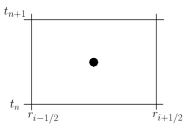
The HRSC picture begins by imagining the plane covered by rectangular cells whose spatial interfaces are spaced apart and reside at half-integer spatial index , and with temporal interfaces spaced apart residing at integer time index . We will work with a schematic equation of the form of Eq. (11.21) where there is a split flux,
| (12.1) |
where we have multiplied through by (which enters the time derivative at no cost), and where are understood to be densitized as in Sec. (11.2). The other hydrodynamic equations (11.16), (11.18) are also of this form if one sets the second flux to zero (and sets the source to zero in the case of Eq. (11.16)).
Integrating Eq. (12.1) over an arbitrary cell, we obtain
| (12.2) |
Note that since the fluid is on a curved spacetime, one should use the proper volume element . However, we can achieve the same result as Eq. (12.2) by pre-dividing by the spatial metric determinant prior to integration.
We now denote spatial averages with a bar, eg.
| (12.3) |
and temporal averages with a hat, eg.
| (12.4) |
One might object that the prefactor in the spatial average should instead be , since this is the inverse volume associated with the domain of integration. We will indeed make this replacement later. Although they differ at , the latter performs better near the origin [121].
We can evaluate certain integrals in Eq. (12.2) using the fundamental theorem of calculus, and the ones we cannot will be spatial or temporal averages so we will denote them using bars and hats. We obtain
| (12.5) |
So far, no approximations have been made, but we do so now. We first approximate the spatial average of the split flux term as
| (12.6) | |||||
where the subscripts , denote evaluation at the corresponding spatial locations. We evaluate spatial averages at cell centres , thus eg.
| (12.7) |
as well as evaluate temporal averages at time (also the cell centre). Eq. (12.5) then becomes
| (12.8) |
Rearranging and replacing , we finally obtain
| (12.9) | |||||
We thus see explicitly here that the evolution of the variable , averaged over the cell, is governed by a flux balance at the cell interfaces and the source terms averaged over the cell. This is why the flux-conservative form of hydrodynamics is convenient for HRSC methods.
Computation of the fluxes is a large subject. Since the variables are defined at cell centres, some interpolation of the variables to the cell interfaces must be done prior to computing the fluxes, and we describe the third-order interpolation we use in the next section (performed on the primitive variables). Let us denote the variables reconstructed from the cell-centred values to the left and right of the cell interface as , respectively. The fluxes themselves are computed using the Harten-Lax-van Leer-Einfeldt [122, 123] (HLLE) formula. If the analytic fluxes themselves are given as functions of as and , then the HLLE formula is given by
| (12.10) |
where are the maximum and minimum values of all the characteristic speeds at and and zero,
| (12.11) |
Since we have a split flux and we do not want to have the term appearing twice, we use for
| (12.12) |
12.2 The piecewise parabolic method
The piecewise parabolic method (PPM) is third-order method of determining the hydrodynamic variables at the cell interfaces, which performs well in reproducing sharp gradients such as the surface of a star. PPM was originally presented in [124]. Other accessible references are [125, 126], which we follow here. In this section, we will describe the method as applied to a uniform 1-dimensional grid, and the reconstruction will be on the primitive hydrodynamic variables.
The method begins with an estimation of the primitive variables at time index and cell interface position index via a quartic polynomial interpolation over the 4 nearest cell centres at position indices , , , :
| (12.13) |
This approximation is fourth-order accurate. However, slope limiters are applied to ensure that is bounded by the two values to the left and right of the interface, . To achieve this, let us first rewrite Eq. (12.13) as
| (12.14) |
where . We then bound by applying the slope limiter [127] to and ,
| (12.15) |
which then completes the estimate as
| (12.16) |
In the next step, we initialize the left and right limiting values at the right interface of cell , written as and , respectively, as
| (12.17) |
We then apply the following replacements, which ensure a monotonic profile for . The first is a reversion to first-order interpolation if the value in the cell centre, , is a maximum or minimum:
| (12.18) |
The second replacement adjusts one of the interface values in the event that an extremum exists within the cell. The result is that the extremum is moved to the opposite interface, and this is done in such a way that the cell-average value is preserved:
| (12.19) | |||
| (12.20) |
Due to these modifications, one order of accuracy is lost, and the method is nominally third-order in smooth regions of the flow away from extrema [126].
There exist additional dissipation and jump-discontinuity steepening algorithms, which we omit. The interested reader can consult the original work for those details [124].
12.3 Primitive variable recovery
The computation of the hydrodynamic fluxes appearing in Eqs. (11.11), (11.12), and (11.14) requires having the values of the primitive variables. In our numerical scheme the conservative variables are evolved, and after each time step the primitive variables must be recovered from the updated conservative variables. In Newtonian hydrodynamics, the conservative-to-primitive variable transformation is algebraic. In the relativistic case, this recovery is delicate due to the presence of the Lorentz factor, and in general a numerical root-finding algorithm must be employed. Using the equation of state, one can write down a function of some variable which depends on the primitive variables, such that the correct values of the primitive variables yield . For example, one could use the pressure and then the root-finding algorithm would find the value of which solves the appropriate equation , and following this the rest of the primitive variables can be computed algebraically.
Most recovery schemes require an initial guess for the root of . In this section we briefly review a bracketing scheme presented in the appendix of [128], which uses causality and energy conditions to calculated upper and lower bounds on the root of a certain function . Following this, the brackets can be narrowed until the root is known to within a desired tolerance. This method is deterministic, in the sense that the transformation is determined entirely by the hydrodynamic data at the current time step, and thus it is reproducible111Although one would also have to use the same error handling policy.. In particular, it does not require an initial guess being provided by eg. the primitive variable values at the previous time step. Here we follow [128] but specialize to the ideal fluid equation of state and spherical symmetry.
We choose our root-finding variable to be . Weighting by the Lorentz factor provides better handling of highly relativistic velocities since is not bounded from above. Using instead makes the recovery procedure vulnerable to numerical errors when .
Begin by defining some auxiliary quantities
| (12.21) |
One can show that , , , , and . We impose that the pressure cannot exceed the total energy density, that it cannot be negative, and that the speed of sound is real and causal:
| (12.22) | |||||
| (12.23) |
However, for the ideal fluid equation of state with , these conditions simply mean
| (12.24) | |||||
| (12.25) |
In the event that the conservative variables have taken on unphysical values, we would like to map them into physical values via an error handling policy. This requires knowing the physical bounds on the conservative variables. For example,
| (12.26) | |||||
Since and , we see that .
Next, one can show that and that . Since is non-decreasing with , we can explore its minimum values by setting , which yields . Thus, . By setting we can explore the maximum possible values of . This gives , which is non-decreasing in over the interval . In this case, to lowest non-trivial order in we have . Thus we have a final ordering inequality given by
| (12.27) |
Therefore . The other inequalities will be used to bracket the root of , to be defined later.
Prior to recovery of the primitive variables, we implement the adjustment policy described in [128], which makes the primitive recovery procedure safe but does not necessarily correspond to physical values. The policy is as follows. If , where is an artificially maintained lower bound on the rest mass density, then all variables are set to the artificial atmosphere values of , . We use a polytropic equation of state to determine , and set to that value as well. Next, if then we reset keeping and constant, which amounts to setting and adjusting such that . Furthermore, if then is rescaled such that , which amounts to setting .
For given values of and conservative variables, we can write and then the rest mass density and internal energy as
| (12.28) |
It is numerically more accurate in the Newtonian limit to replace with , and we do so. Once and are obtained, one can obtain via the equation of state and then the enthalpy . Then the velocity is recovered via
| (12.29) |
We find the root of the function
| (12.30) |
which comes from the definitions of our auxiliary quantities above, where we use . During recovery, Eqs. (12.28) may yield values outside of the physical range. Thus for a given value of (and given conservative variables), after computing the candidate values of and we map them into the physical range via
| (12.31) |
prior to computing . The bracketing Eq. (12.27) implies that the root of is bounded above and below by
| (12.32) |
With these bounds given, a root-finding algorithm such as bisection or regula falsi will converge to the solution. We use the Illinois algorithm, which is regula falsi with an additional conditional step designed to circumvent slowly-converging situations.
Once the recovery is finished, we impose the atmosphere values on any points with or , and adjust any velocities with to , where is a specified parameter (0.99 in our case).
12.4 Boundary injection of hydrodynamic pulse
Since we have done the work necessary to control the boundary conditions, we can obtain fully dynamical evolutions by using stationary black hole solutions as initial data and then inject matter into the domain through the outer boundary. In this section we will see that we can inject a hydrodynamic pulse by setting the velocity to zero at the outer boundary, and control the injection speed with the specific internal energy .
Looking at the hydrodynamic characteristic speeds Eq. (11.24) and setting the velocity to zero yields
| (12.33) |
With this choice, both and are ingoing modes. Whether is ingoing or outgoing depends on the sound speed (and coordinate conditions). With zero velocity the hydrodynamic characteristic variables Eq. (11.30) reduce to
| (12.34) |
Thus in this zero velocity limit the characteristic variables are degenerate, with the amplitude of the injected pulse controlled by while the injection speed is controlled by . We can control via through the relation
| (12.35) |
In simulations where the shift vector is zero, we will also prescribe a non-zero value of the velocity in order that the material wave velocity be nonzero and ingoing.
12.5 PN solver
After a hydrodynamic update, the metric variables are solved for via the PN Eqs. (11.74) and (11.75). Since the primitive hydrodynamic variables appear on the right-hand sides, a transformation from conservative to primitive variables is necessary before the PN equations can be solved. To do this, we use the procedure described above in Sec. (12.3).
However, this transformation itself requires the updated metric component for raising and lowering indices of and . Therefore we use the last available values of for the primitive variable recovery.
The PN equations (11.74) and (11.75) are reduced to first-order in space by defining
| (12.36) |
The Laplacian in spherical symmetry is , and the PN equations (11.74) and (11.75) become
| (12.37) | |||||
Eqs. (12.36) and (12.37) are integrated radially out from the origin using LSODA [129], which is implemented in Fortran in ODEPACK [130] and wrapped in Python in the Scipy package [131]. This routine takes internally defined steps, and we use linear interpolations of the right-hand sides to accommodate this. We use boundary conditions at the origin , since in spherical symmetry these variables have no information about material at greater radii. I.e. If there is no matter at greater radii, the integration should yield everywhere.
With this solution scheme, and treating the time derivative terms in Eqs. (12.37) with backward stencil finite differences, we experience the development of instabilities over time. This is due in part to the fact that we interpolate the right-hand sides in order to accommodate the internal steps of the solver. Resolving this issue will require more careful discretization of the equations, the use of a lower-order integration method less sensitive to interpolation errors, and possibly evolving the fluid on a finer grid than the PN potentials. Without having this issue resolved at our current stage, we instead turn off the time derivative terms entirely. We monitor those terms, computed during post-processing, to gauge how important they are, although the solution itself in this case is not correct so this monitoring is not necessarily reliable either.
Once and are solved for, they are added to (Eq. (11.73)) and . We also have . Using these potentials, the ADM variables are computed for use in the next time step in the hydrodynamic equations.
12.6 Further code details
We use a 3rd-order accurate Runge Kutta time stepping scheme that is total variation diminishing (TVD) [132], which means the point-to-point spatial variability of solutions does not increase in a global sense over time. For some variable governed by an equation for some operator , the scheme is presented as (eg. [133])
| (12.39) | |||||
Here, the superscripts n and n+1 denote times, whereas (1) and (2) denote intermediate values at substeps.
Spatial derivatives of graviational variables are performed with 2nd-order centred finite differences which reduce to 1st-order at boundaries such that they satisfy summation by parts [134]. This is required to avoid artificially injecting energy into the grid. In the interior of the grid, the difference operator is
| (12.40) |
while at left and right boundary points the difference operators are, respectively,
| (12.41) |
Here the subscripts j indexes spatial points.
For suppressing unresolved high-frequency, short-wavelength noise in the gravitational variables in the GR fluid code, we employ Kreiss-Oliger dissipation [42] that is 4th-order in the interior of the grid and 2nd-order at the boundaries [134]. This is essential for stability of the code. The choice of 4th-order dissipation does not affect the accuracy order of the derivative operator above. The dissipation term is
| (12.42) |
where we fix for all GR fluid simulations. This term is added to the right-hand side of the evolution equations for each variable.
Chapter 13 Code validation
13.1 Artificial analytic convergence test of the hydrodynamic solver
In this test, we perform an artificial analytic convergence test of the hydrodynamics solver. This means choosing arbitrary space- and time-dependent functions for the hydrodynamic variables, plugging them into the equations of motion to obtain new source terms, then including those new source terms on the right-hand side of the hydrodynamic evolution equations in the solver. This forces our arbitrary choice of functions to be an analytic solution to the new system, and we can perform convergence tests against this artificial analytic solution. The new source terms are computed independently from the code, so as not to contaminate the test with possible errors in the code itself, and the arbitrary functions we choose are demanding for the solver.
This test can be made as demanding as one wishes, unlike the options available via other analytic solutions which are often time-independent or special in some way. We choose to make the test very demanding by including time- and space-dependence in the fluid variables and the metric.
The artificial solution we choose is written as
| (13.1) | |||||
| (13.2) | |||||
| (13.3) |
where is the physical size of the domain, produces an oscillation in amplitude ( is the total integration time ), and produces an oscillation in position. These frequencies are chosen to have irrational ratios so that they are not commensurate [135]. As far as the physical appearance of this solution, it is a Gaussian pulse of width whose position is oscillating between , and with a rest mass density peak amplitude oscillating between . It is important to note that the way the pulse travels is not at all determined by our choice of , because a counteracting source term is added to the hydrodynamic equations which cancels its influence (to within the accuracy of the solver).
In order to test the dependence of the densitized variables coming directly from a varying metric, we also need to prescribe a time- and space-dependent metric (see Eqs. (11.19) and (11.20)). We therefore impose that the spacetime metric is that of a Schwarzschild black hole in isotropic coordinates, with a mass varying sinusoidally in time between with a frequency . This turns on terms in the hydrodynamic equations involving , , and their space and time derivatives.
We also note that since the tails of the pulse approach the atmosphere values, the atmosphere algorithm is employed heavily there, resulting in a particularly demanding test.
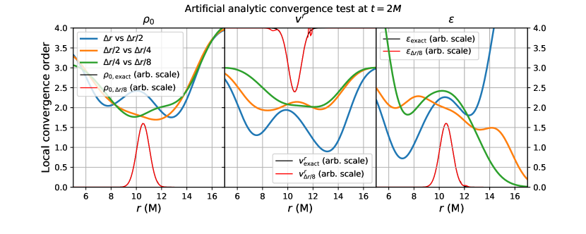
We display the results of this artificial analytic convergence test in Fig. (13.1). Local convergence factors are plotted versus radius at a representative time for the primitive hydrodynamic variables (Left), (Centre), and (Right). For a given resolution , the factors are given by
| (13.4) |
for , as an example, where the subscripts and denote the solution obtained with those resolutions. The absolute value is taken at a specified time. In Fig. (13.1) the fiducial resolution is . The convergence factors are also smoothed with a Gaussian of width , which removes uninformative very short-wavelength noise from the plots. We see convergence averaging around an order of in the bulk of the fluid pulse, consistent with the numerical methods. In the outer tails of the pulse, the convergence order observed is not representative of the method. We attribute this to the densities being extremely low there, comparable with the atmosphere value, and thus invocations of the atmosphere algorithm are more common.
It is important to keep in mind that this metric is not physical, but it does not have to be for this test. We are simply manufacturing enough dynamics in order to test the convergence of the hydrodynamic solver in a thorough way. The spacetime evolution equations are not employed in this test, rather the metric is prescribed at each time. The spacetime evolution will be tested in later sections.
13.2 TOV oscillations in the Cowling approximation
In this test, we evolve a TOV star with central density , obeying an initial equation of state with and adiabatic index , which yields a star with a radius km if we take . This choice of parameters has been used in the literature to test codes and the mode frequencies have been repeatedly obtained, eg. [136, 137, 138, 139]. They can also be obtained with perturbative calculations [140]. We perform this test in the Cowling approximation (fixed spacetime) in Schwarzschild-like coordinates. Performing this test with a dynamic spacetime requires regularization of the gravitational equations at the origin, which we have not implemented. In our main application we have the origin excised out of the grid due to a black hole there, so regularization is not an issue. Thus, this test should be regarded as a physical test of the hydrodynamic solver, without the time-dependent metric source terms being activated.
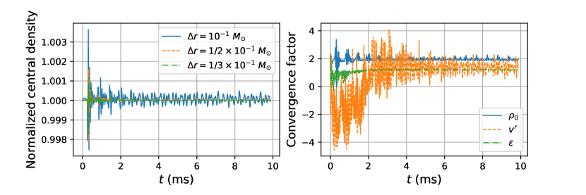
Fig. (13.2) displays the time progression of the normalized central density of the star for different resolutions (Left). Although the TOV solution is static, truncation errors during its numerical evolution excite the normal modes of the star. The global convergence factor in an norm sense is also displayed (Right) for the primitive hydrodynamic variables , , . The norm is taken over the entire interior of the star. We observe second-order convergence for the density, and degraded convergence of order for the remaining variables after ms. There is a transient phase during first ms when the velocity exhibits apparent non-convergence. We attribute this to the fact that the surface of the star is truncated at different radii for different resolutions, and each star must settle down from these slightly different initial configurations. Difficulties with the star-vacuum interface and the associated convergence issues are well-known for finite volume methods, see for example [142].
In Fig. (13.3) we display the frequency spectra of the central density of the star for different resolutions. To produce these plots, we first subtract from its average value over the whole duration ms. Secondly, since there exists an initial burst at visible in Fig. (13.2) (Left), we decrease its contamination of the spectra by multiplying the time series by a Gaussian window function . The offset of ms and width of ms are chosen simply to retain the central part of the time series while excluding the outer edges in a smooth manner. The windowed time series is more closely represented by a periodic function, and thus produces cleaner Fourier spectra. Similar methods are employed elsewhere, eg. [143, 139]. Then we compute the spectra and normalize them to 1. Also overlaid in Fig. (13.3) are vertical lines indicating the frequencies of the fundamental mode and its first six overtones , which were found in [137] to be kHz, respectively.
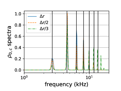
13.3 Ingoing gauge pulse
In this test, we inject a gauge pulse into the domain of a static black hole and observe whether the gauge-invariant Misner-Sharp mass is unaffected at the order expected from the numerical method used. This pulse is a purely coordinate degree of freedom, thus no physical quantities should vary.
The gauge pulse consists of a Gaussian superposed on top of the Painlevé-Gullstrand value of the characteristic variable at the outer boundary. We implement this at the level of the right-hand side of , which is zero in Painlevé-Gullstrand coordinates. The modified right-hand side is
| (13.5) |
We choose the pulse parameters to match those chosen in [116]. Namely, , , . Furthermore, the boundary is located at and we evolve until , using three different resolutions , , .
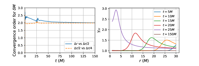
In Fig. (13.4) we plot the global convergence order for the Misner-Sharp mass in an norm sense (Left), and a time progression of from the most resolved run. The fiducial resolution is in the (Left) plot. The convergence order is observed to approach .
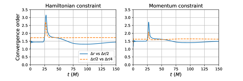
In Fig. (13.5), we display the convergence order of the constraints in an norm sense, yielding in the most-resolved case. A spike occurs when the gauge pulse exits the domain through the excision surface, where gradients are high and the errors grow.
13.4 Ingoing hydrodynamic and gauge pulses
In this test, we place the outer boundary at and evolve a black hole of initial mass until . A hydrodynamic pulse is injected through the outer boundary by imposing
| (13.6) |
which is a pulse profile with rise and fall, with a constant duration at max amplitude for a time . The specific internal energy is chosen to be
| (13.7) |
and the pressure is determined from the ideal gas equation of state with , and for simplicity. For these tests, we choose and , which gives a rise duration of , a constant duration of , followed by a fall duration of . The amplitude is chosen as . This pulse results in a final black hole mass of , a 21% increase.
In one case, we inject only the hydrodynamic pulse. In another more demanding case, we also inject the same gauge pulse defined in Sec. (13.3), but delayed so that the peak occurs at . This delay is done to reduce the overlap of the hydrodynamic and gauge pulses at the boundary, although the overlap is still non-zero there since the gauge pulse is Gaussian. The pulse is also different than the previous test in that it is injected at rather than , as in Sec. (13.3).
Fig. (13.6) shows a time progression of the areal radius of the apparent horizon (Left) and the rest mass density of the fluid (Right). Solid lines correspond to the case with an ingoing hydrodynamic pulse only, while dashed lines correspond to the case with consecutive hydrodynamic and gauge pulses. The apparent horizon radius is defined implicitly by , and is coordinate-dependent. The gauge pulse affects the evolution of the coordinates, so it is expected that it would produce a modified evolution of the apparent horizon. However, after the black hole has absorbed everything, both cases settle down to the same black hole mass (Left). There is a slight discrepancy apparent in the hydrodynamic pulse profile at between the two cases (Right). This is partly due to a disagreement between the radial coordinates in the two cases; plotting vs the areal radius for both cases increases the coincidence of the two pulse profiles. However this does not completely account for it, and the remaining disagreement we attribute to a combination of different hypersurface evolution and a physical difference between the injected hydrodynamic pulses arising from the non-zero overlap between the hydrodynamic and gauge pulses at the boundary (since the latter is a Gaussian and so never vanishes). Such an overlap modifies the lapse and at the outer boundary, which from Eq. (12.33) affects the fluid characteristic speeds there, which can result in a slightly different pulse profile. This small difference would magnify as the fluid enters the black hole around , where volume decreases and the fluid velocity reaches .
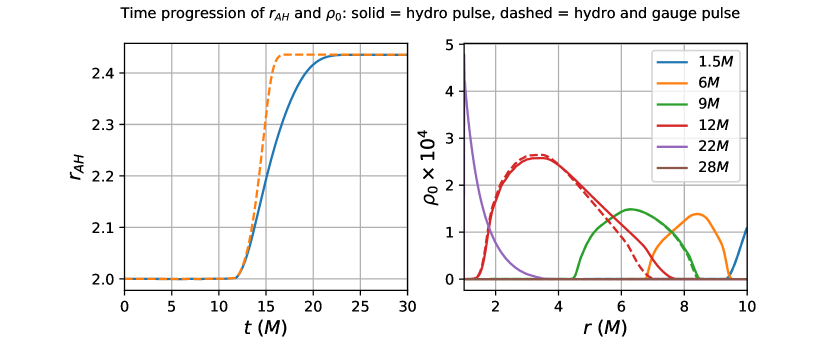
In Fig. (13.7) we plot the global convergence order in an -norm sense for the constraints. The analytic solution would have vanishing constraints, so this is an analytic convergence test rather than a self-convergence test. Again, solid lines correspond to the case with a hydrodynamic pulse only, whereas dashed lines also include the gauge pulse. When the error is dominated by the hydrodynamic solver, we obtain the expected convergence order of . We observe that when the gauge pulse propagates through the grid, the error changes significantly such that between the convergence order increases to . Note that this does not mean that the errors have decreased, only that the convergence order has increased; one expects that the errors are larger during this time, and some other truncation error term beyond the lowest one is momentarily dominant.
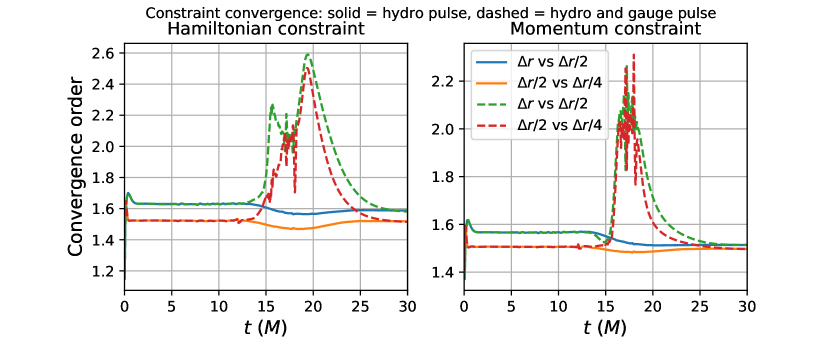
Finally, in Fig. (13.8) we display second-order convergence of the change in black hole mass between the beginning and end of the simulations. This is a test to see whether the black hole grows by the expected amount, based on how much fluid it absorbs. The difference we are plotting is
| (13.8) |
i.e. a comparison between the change in black hole mass according to the Misner-Sharp mass evaluated at the outer boundary at the initial and final times, and the total proper ADM mass of the hydrodynamic pulse,
| (13.9) |
at when it has first completely cleared the outer boundary. As expected, the errors are larger for the more demanding case with a large gauge pulse (orange circles).
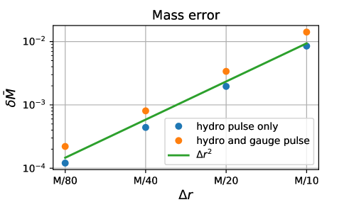
13.5 Hydrodynamic pulse with PN gravity
In this section we test the PNGhydro code with a fluid pulse initialized on the computational grid. We have a “PN black hole” of mass present (i.e. a black hole approximated to some PN order), and the computational domain extends out to . The black hole PN potentials are obtained from [144, 84] by setting the spin parameter to zero, since we are in spherical symmetry. This yields
| (13.10) | |||||
The initial profile of the fluid corresponds roughly to an ingoing pulse [145], which is conveniently specified and easily implemented in terms of the conservative variables as
| (13.11) | |||||
| (13.12) | |||||
| (13.13) |
The choice of is the crucial aspect of this choice which reduces the outgoing part of the pulse. This was observed in [145] in simulations, where an initially stationary pulse splits into ingoing and outgoing pieces with and , respectively. One expects this would be reflected at the level of the characteristic variables as well, as in Sec. (11.3).
We evolve this initial setup for a total time and perform an independent residual test on the simulation output. This means that we write an independent script, without any reference to the simulation code, which evaluates the left- and right-hand sides of the PN equations based on the code’s output. The difference between the left- and right-hand sides is analytically known to be zero by virtue of the equations. Thus, when computing convergence factors in an independent residual test, one only needs two resolutions. We denote the residual in eg. the case as
| (13.14) |
and the convergence factor will be
| (13.15) |
where by virtue of Eq. (11.74). This is therefore a form of an analytic convergence test. Our fiducial resolution is . We also only solve for the PN potential , which means we are restricting to coordinates where (which can always be chosen in spherical symmetry).
Fig. (13.9) shows the results of this test: (Left & Centre) show global self-convergence of the lapse and rest mass density to indicate a reference level of convergence. Self-convergence requires three resolutions, and we use . (Right) shows the independent residual test, yielding a convergence order .
Thus, although our solution method interpolates the right-hand side of Eq. (11.74) for the internal steps taken by ODEPACK (which introduces errors), we obtain reasonable results. We will improve the solution method in future efforts, but we present preliminary results with the current code below.
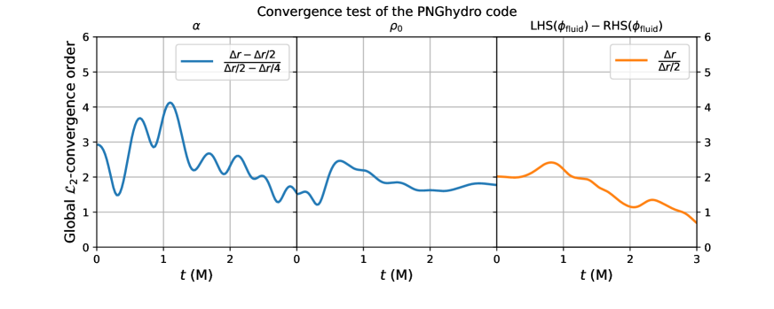
Chapter 14 Preliminary results & future work
Here we present preliminary results, wherein we simply compare the evolutions of the same system in both the GR fluid and PNGhydro codes. Since the black hole PN potentials in Eqs. (13.10) are just truncated expansions of a Schwarzschild black hole in isotropic coordinates, we use the exact black hole in isotropic coordinates as the initial data for the GR fluid run. We place the outer boundary at , use a resolution , and evolve for a total time of .
The rest mass boundary data as a function of time is given by Eq. (13.6), except with no constant duration at max amplitude (i.e. ), and with amplitude . This again is a rise and fall, and the parameter yields rise and fall times of , so that the pulse clears the boundary at . The specific internal energy at the boundary is chosen to be
| (14.1) |
As mentioned at the end of Sec. (12.4), since the shift vector is zero in isotropic coordinates, the material wave velocity () will be zero unless we choose a non-zero . We therefore prescribe the boundary value of in units of as
| (14.2) |
which thus turns off in a fashion commensurate with beginning at when the boundary rest mass reaches maximum amplitude. These boundary parameters result in the injection of a fluid pulse of total mass .
As in Sec. (13.5), we set , which corresponds to a coordinate choice. Since our goal is to test the PN formalism in a numerical implementation, we would ideally not make this choice, so that we can test all of the PN equations. However, given that our GR fluid implementation uses an a priori-specified shift vector, we cannot possibly specify the shift in accordance with what the PNGhydro evolution is representing since we do not know what it is. This difficulty only exists for this simple side-by-side comparison of the evolutions; in future explorations we will compare coordinate-invariant quantities so that these issues do not arise.

In Fig. (14.1) we display the temporal progression of the hydrodynamic quantities (Left), (Centre), and (Right). All quantities are plotted versus the areal radial coordinate, . In (Centre), we also display the rest mass density profiles at the bottom of the plot in dotted lines, so as to indicate where the bulk of the fluid is at each time. The kinked portions of the velocity occur at the bow of the pulse, where there exists a small shockwave with rest mass amplitude near the atmosphere level . At lesser radii the velocity increases, which is simply due to the atmosphere accreting towards the black hole. In (Right), the specific internal energy is observed to have poor agreement between the GR fluid and PNGhydro runs in the bulk of the pulse. However, the larger values in the shock-heating region of the aforementioned small shockwave agree well (large rectangular features).
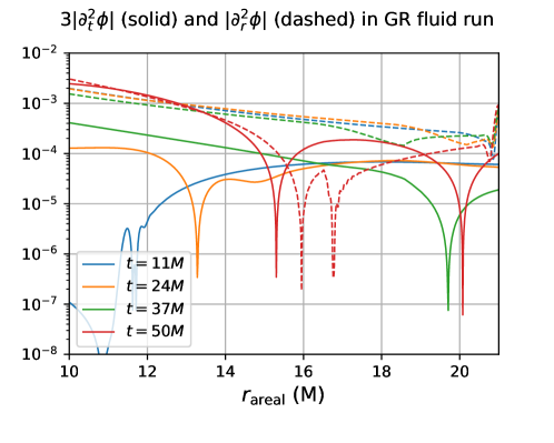
As we explained in Sec. (12.5), we have set the term to zero on the right-hand side of Eq. (11.74) due to numerical difficulties. In Fig. (14.3) we assess the degree to which this has affected the evolutions we obtained in this section. Using the GR fluid run, we transform from ADM metric variables Eq. (11.36) to the PN potentials Eq. (11.66). This yields PN potentials which are more accurate than the PNGhydro output would yield, since they come from solving the full Einstein equations without any PN approximations. We then numerically compute and using 2nd-order centred finite differences, in order to compare their magnitudes. We plot the absolute value of these derivatives in Fig. (14.3), and observe that at all times except the final time , the spatial derivatives have a larger magnitude than the time derivatives by a factor of . This gives a sense of how large the omitted term is on the right-hand side of Eq. (11.74) for this particular evolution.
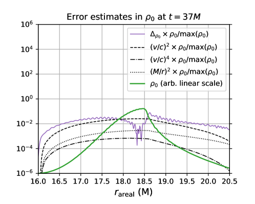
Lastly, in Fig. (14.3) we compare the relative error in at , defined via
| (14.3) |
and the expected error coming from the order at which the PN expansion has been truncated. Since the PN expansion is a simultaneous expansion in and , we plot various contributions in black: the 0PN error (i.e. the error expected if computations are done at 0PN), the 1PN error , and the 1PN error111 is in the context of circular orbital motion. However, our fluid is undergoing spherical collapse, so can differ significantly from . . All errors are normalized by in order to suppress the less important errors at the tails of the pulse, which can be quite large otherwise. The pulse profile itself is also shown on an arbitrary linear scale, to indicate its position and where the peak is. We see that the error in the pulse due to the PN treatment is well-matched by the 1PN compaction error near the peak of the pulse around . Elsewhere the error is larger, which we will investigate during future efforts to improve our PNGhydro code.
Once we have overcome the numerical difficulties in treating the time-derivative terms in the PN equations (11.74), (11.75), we will proceed to implement the higher order 2.5PN equations derived in [84]. It is these higher order approximations which have yielded a marked improvement in eg. the mass-radius curve for cold neutron stars [84]. Thus the prospect for improving pseudo-Newtonian simulation codes via this PN formalism remains an exciting possibility.
Part III Mode structure of rotating core-collapse supernovae
Executive summary
In this part, we show that asteroseismology of rotating core-collapse supernovae is possible with a multimessenger strategy. Using a standard stellar model with zero-age main sequence mass with rad/s pre-collapse central rotation, we show that an , oscillation mode of the newly-born rotating proto-neutron star with frequency Hz is responsible for a correlated peak emission frequency in both gravitational waves and neutrino luminosities. We achieve this by first identifying the mode in the non-rotating model via an eigenfunction matching procedure between the full nonlinear simulation and a perturbative calculation. Then we follow the mode along a sequence of rotating models by establishing the continuity of its eigenfunction. For an initial pre-collapse rotation rate of rad/s, the correlated frequency of gravitational wave and neutrino luminosity emerges. We show that the dominant angular harmonics of the emission pattern of neutrinos on the sky are consistent with the mode energy in a shell around the neutrinospheres, where km. Thus, the neutrinos carry information about the mode in the outer region of the proto-neutron star where km, whereas the gravitational waves probe the deep inner core km.
![[Uncaptioned image]](/html/1810.04594/assets/x30.png) Figure III: Preview of the , , mode, whose frequency mask is overlaid on the gravitational wave and neutrino spectrograms from our sequence of rotating models. The models are parameterized by pre-collapse rotation rad/s. Here we see that the mode is coincident with dominant bands in the rad/s case across all messengers.
Figure III: Preview of the , , mode, whose frequency mask is overlaid on the gravitational wave and neutrino spectrograms from our sequence of rotating models. The models are parameterized by pre-collapse rotation rad/s. Here we see that the mode is coincident with dominant bands in the rad/s case across all messengers.
Chapter 15 Introduction
The collapse and bounce of the iron cores of massive () stars and the possible ensuing supernovae are expected to produce detectable gravitational waves and neutrinos if they occur within or very near our galaxy. Indeed, neutrinos have already been detected from such an event, named SN1987A [146, 147]. Events with a successful explosion are called core-collapse supernovae (CCSNe). The electron-degenerate iron core collapses once it exceeds the Chandrasekhar limit, and unless it is very massive the collapse will be halted once the core reaches nuclear densities g and its equation of state stiffens. This sudden halting imparts momentum to the supersonically infalling stellar material, causing a powerful outward shockwave. Whether and how this shockwave and the subsequent dynamics results in a successful explosion is a central theme of research in this area.
In the event of a successful explosion, as in SN1987A, photons are also detectable. In contrast with photons, which are heavily reprocessed before freely streaming to an observer, the intervening stellar material between the core and an observer are transparent to gravitational waves. The star is also largely transparent to neutrinos, except for example within several dozens of kilometres of the centre of the core and within tens of milliseconds after core bounce, where scattering is still strong. Neutrinos and gravitational waves therefore offer deep probes of the central engine of a CCSN.
Interestingly, correlated frequencies between gravitational waves and neutrino luminosities have been observed in simulations within tens of milliseconds after core bounce in [148]. Similar correlations at later times have been reported in [149], likely due to the growth of the standing accretion-shock instability (SASI). These observations point towards a wealth of opportunity to probe specific aspects of the central dynamics occurring at different times, from tens of ms to several seconds and beyond.
Asteroseismology is the study of the interior structure of stars inferred from observations of its seismic oscillations. There have been some very recent efforts to use gravitational waves to do the same with CCSNe, so-called gravitational wave asteroseismology [150, 151, 152, 153]. The main strategy is to use data from numerical simulations as input for a perturbative mode calculation, where the simulated data serves as a background solution. The key point to note is that there is a separation of scale between the period of the modes of interest and the time scale over which the post-bounce CCSN background changes significantly. For example, towards the pessimistic end, a Hz mode has a period of ms, whereas the CCSN background changes over a timescale of several tens of ms. Therefore one expects to be able to treat the CCSN background as stationary for the purposes of a perturbative calculation at any instant of time. In [150] this was done using a perturbative Newtonian hydrodynamic scheme in an effort to generate a qualitative understanding of the gravitational wave emission due to the oscillations of a rotating proto-neutron star that were excited at bounce. Subsequently, [151] presented a similar effort using perturbative hydrodynamic calculations in the relativistic Cowling approximation. Shortly thereafter, and during the course of this work, [152] partially relaxed the Cowling approximation by allowing the lapse to vary, governed by the Poisson equation. They claimed an improved coincidence between their perturbative mode frequencies and certain emission features in the gravitational wave spectrograms from simulations. The Cowling approximation was then relaxed even further in [153], where the conformal factor of the spatial metric was allowed to vary as well, leaving only the shift vector fixed.
All of these studies, however, attempt to identify specific modes of oscillation of the system primarily by coincidence between perturbative mode frequencies and peaks in gravitational wave spectra, across time. This is potentially problematic for a number of reasons. Firstly, the approximations used in the perturbative calculations introduce errors in mode frequencies that can be quite significant, eg. several tens of percent in the case of lower order modes in the Cowling approximation. Secondly, any partial relaxation of the Cowling approximation presents difficulties with the interpretation of results, since this strategy neglects some terms at a given order but not others, and thus is not a priori under control. Thirdly, the approximations used in the simulations themselves introduce their own frequency errors. For example, as had motivated our efforts in Part (II) to improve gravity treatments in some codes, gravity is often treated in a pseudo-Newtonian manner in CCSN simulations by modifying the potential to mimic relativistic effects, as in [152, 94, 154]. The mode population in the vicinity of a given frequency bin in a gravitational wave spectrum can be rather dense, therefore all these sources of error serve to lower the significance of any given observed coincidence between perturbative and simulated mode frequencies. Indeed, the purported identification of a -mode in [154] required a post hoc modification of its frequency formula when matching to gravitational wave spectrograms from simulations.
We opt to take a different approach. Rather than looking for coincidence in mode frequencies, we look for coincidence in mode functions. This means comparing mode functions, obtained from perturbative calculations, with the velocity data from simulations, which are heavily post-processed using spectral filters and vector spherical harmonic decompositions. We will find that if a mode has an adequate excitation, its matching with candidate perturbative mode functions is unambiguous. Since this strategy does not use frequency-matching, we will also discover a shortcoming of our simulation code: the frequencies observed in our simulations are significantly overestimated, with the true values being at least % lower. This illustrates the power of matching in mode functions rather than mode frequencies, and bears out our concerns with focusing only on mode frequency coincidence as in [151, 152, 153].
We use the perturbative scheme in the relativistic Cowling approximation from [151], which applies only to spherical systems. Therefore we will only apply it to a non-rotating model in order to identify modes of oscillation that are excited at bounce and ring for ms. This identification serves to label the corresponding modes in the rotating models [155] whose mode functions deformed continuously with increasing rotation, picking up a mixed character in angular harmonics. We also simulate a sequence of rotating models with progressively larger pre-collapse rotations of rad/s. In order to follow the modes along this sequence, we take inspiration from the works of [136, 156, 157]. In [136], knowledge of the modes of the non-rotating star were combined with continuity in frequency to follow modes across such a sequence, whereas in [156, 157] continuity in mode functions was used. Continuity in mode function is more powerful than continuity in frequency, since separate modes can have very similar frequencies and thus would be degenerate in a continuity analysis. Thus we will chiefly use mode function continuity to follow modes along our sequence of rotating models.
A powerful method in [156] called mode recycling was used to converge toward the mode function of rotating stars. One simulates the star with an initial perturbation corresponding to an educated guess for the mode function of interest, which due to its inaccuracy will excite several unwanted modes. By applying spectral filters to the velocity field in the star, a more accurate trial mode function for the target mode can be extracted and used as an initial perturbation in a second simulation. This process is repeated until the initial perturbation results in a clean excitation of the target mode, with unwanted modes highly suppressed. The strategy of mode recycling is not available in our context, since our target modes are excited by core bounce, which we do not attempt to manipulate. Thus we rely strictly on mode function continuity, but we will employ a suite of known facts about the possible deformations of modes in the slow-rotation regime in order to bolster our analysis.
Our chief result will be the implication of an , mode with at least 2 radial nodes in the production of correlated gravitational waves and neutrinos in the rad/s model. In contrast with [148] where the neutrino treatment did not supply information about the emission pattern on the sky, our treatment does allow this. We will relate the dominant angular harmonics of the emission to the dominant energy harmonics in the mode function in the vicinity of the neutrinospheres. The causal explanation for the oscillations in the neutrino luminosity will be that the mode of the proto-neutron star, which in the rotating rad/s model has a mixed character in , is producing and variations in the shape of the neutrinospheres. Since the neutrinospheres are roughly the boundary between trapped and free-streaming neutrinos, this means that the region producing free-streaming neutrinos is undergoing variations in shape in accordance with the activity of the mode in the vicinity of the neutrinospheres, at km. This causes the oscillations in neutrino luminosity registered by an observer far away. We therefore find that detailed asteroseismology of CCSN is possible with joint detection of gravitational waves and neutrinos, where the neutrinos supply information from the neutrinosphere region km, and the gravitational waves supply information from deeper in, around km where the bulk of the mode energy resides.
This part is organized as follows. In the next section (15.1) we will review the necessary background material and terminology from the theory of oscillations of stars required to understand this work. Chapter (16) will contain a description of our simulation code in Sec. (16.1) and the perturbative schemes of [151, 152] in Sec. (16.2). We will describe the process of extracting modes from our simulations in Sec. (16.3). Mode tests of our perturbative schemes and our simulation code will be performed on a stable TOV star in Secs. (16.4) and (16.5), respectively. We will find that the scheme of [152], which we dub the partially relaxed Cowling approximation or simply the partial Cowling approximation, is significantly less accurate than the Cowling approximation itself for fundamental mode frequencies, and even fails to reproduce the correct radial order of high-order modes. In Chapter (17) we present our results concerning the , , mode and its associated signatures in gravitational waves and neutrinos for the model with pre-collapse rotation rad/s. We conclude in Chapter (18), and display mode-matching for many other modes in the non-rotating model in Appendix (A).
15.1 Background and terminology
In this section we review some basic facts and terminology surrounding the mode structure of stars which we will use in our analysis to characterize modes. We will follow [155].
Hydrodynamic perturbations consist of scalar and vector parts, which can be decomposed angularly using spherical harmonics . Scalar perturbations admit expansions in the spherical harmonic functions themselves, whereas vector perturbations admit expansions in vector spherical harmonics. The vector spherical harmonic basis is
| (15.1) |
In general the last two members of this basis will have both and components, but in axisymmetry () the situation simplifies: the vector spherical harmonic basis splits up into components,
| (15.2) |
In spherical symmetry, the modes of stars split up into separate spherical harmonics , with an additional radial order specified by , which is a count of the number of nodes in the radial part of the mode function. An -mode with no nodes () is called a fundamental mode, and its companions are called overtones. Furthermore, in spherical symmetry modes are degenerate in in the sense that modes with the same but different have the same frequency. Rotation breaks this degeneracy, and mode functions no longer split up into different but rather become superpositions of arbitrarily many different spherical harmonics. The possible deformations of axisymmetric modes of rotating stars (relative to the same modes in the non-rotating star) are tamed via their parity-definiteness, which we explain next.
There are different notions of parity which should be understood. A spherical harmonic function behaves under a parity transformation (or ) as
| (15.3) |
The first notion of parity is whether a sign change occurs under parity inversion. Thus, we say that has even parity for even and odd parity for odd . However, the even or odd parity of is not preserved when moving to the vector spherical harmonics; and will preserve the even or odd parity of , whereas will invert the parity due to the presence of the curl operation. Thus, for example, in axisymmetry if a mode function is a superposition of even- terms and odd- terms , then it has even parity. Conversely, if a mode function is a superposition of odd- terms and even- terms , then it has odd parity.
The second notion of parity is relative to . Namely, if a member of the vector spherical harmonic basis for a given has the same parity as , then it is said to have polar parity. Conversely, if the member has the opposite parity of , then it is said to have axial parity. Thus, for example, in axisymmetry a mode with definite even or odd parity could be a superposition of both polar and axial terms, but all axial terms will be and all polar terms will be .
As mentioned above, an important fact we will use in our analysis is that axisymmetric modes have definite even or odd parity. Thus, an axisymmetric mode of a rotating star cannot be a mixture of even- terms and , for example. In our simulations below, axisymmetry is enforced exactly, so we can use the parity-definiteness of axisymmetric modes to help determine whether two -terms are part of the same mode function.
There is a convention for labelling modes of rotating stars. First note that modes of rotating stars deform continuously as a function of the rotation rate . In most cases, a mode of a rotating star deforms to a single spherical harmonic in the limit111So-called hybrid modes have frequencies which go to zero in the non-rotating limit, while the eigenfunction is a superposition of different s [155]. The convention is to label the mode in the rotating case according to what it deforms to in the non-rotating limit. For example, the “fundamental mode” of a rotating star (a so-called quasi-radial mode) may in fact have terms in its mode function, which would allow it to radiate gravitational waves, and may in fact have radial nodes – but in the non-rotating limit it is purely and and nodeless. Note that strictly speaking one must specify a sequence of rotating stars in order to talk about a mode’s deformation as a function of , for example a sequence of fixed rest mass or of fixed central density, and one can observe different qualitative behavior of the modes along such sequences.
The deformations of mode functions of rotating stars are further restricted under the condition of slow rotation. Polar -modes of non-rotating stars receive deformations by axial -terms at such that is odd, and receive deformations at the next order by polar -terms such that is even. Conversely for axial -modes of non-rotating stars: polar deformations at with even, and axial deformations at with odd. Notice these deformations preserve even or odd parity.
Lastly, axial modes of non-rotating stars ( in axisymmetry) have zero frequency (stationary flows), and their frequency increases linearly with the rotation rate of the star in the slow-rotation limit. Such modes are called -modes since their oscillations are rotationally supported by the Coriolis force. In our simulations, such modes cannot be excited in the non-rotating case because the velocity in the direction is exactly zero, but they may be excited in rotating cases.
Chapter 16 Implementation
16.1 FLASH implementation [94]
We will be performing multi-physics simulations, which is necessary for the study of CCSN. To this end we use a mature, modular code base which has applications in many areas, which we describe now.
We use the FLASH111http://flash.uchicago.edu code [158, 159] version 4, which is a publicly available massively parallel modular code which simulates compressible Newtonian flows. It supports adaptive mesh refinement, and is applied in many distinct settings with various extensions. The development of FLASH has focused on modularity and extensibility, with application-specific enhancements made possible without an alteration of the core code.
In the hydrodynamics solver, the variable reconstruction at cell interfaces uses the piecewise parabolic method, as in Sec. (12.2). Since different flux formulae have different strengths and weaknesses, the fluxes are treated with a hybrid method which reverts to HLLE as the lower-accuracy option.
The gravity and hydrodynamics treatments are Newtonian, however an “effectively” general relativistic potential obtained through phenomenological considerations and tested in -dimensional CCSN evolutions has been introduced in [160, 161, 93] and implemented in FLASH in [94]. This is a correction to the monopole term in the potential, and helps to recover the structure of relativistic stars in spherical symmetry.
The neutrino physics is too costly to implement without approximations, since it involves solving the Boltzmann problem for a very large number of particles. Such a calculation is limited by the large dimensionality of phase space, and many different approximate treatments have been employed in the literature. We use one of the better treatments available, the M1 scheme [162], which evolves the moments of the neutrino distribution function with an analytic closure in which the first two moments (average and variance) carry all of the information. This treatment evolves neutrino fields on the computational grid, and thus allows us to extract the directional emission of neutrinos, which will play an important role in this work. Directional emission of neutrinos was not available in similar earlier studies due to the use of cruder neutrino treatments which yield only isotropic emission (the so-called leakage scheme) [148].
A full description of this code is beyond our scope, so we refer to the references [158, 159, 162, 94] for more details.
Seeing as our simulations use pseudo-Newtonian gravity, gravitational waves (GWs) are not actually present on the grid. We instead extract a GW signal using the quadrupole formula [163]. This approach has been tested in the context of rotating stellar core collapse in [164].
16.1.1 Stellar models
The models we evolve come from the widely used stellar evolution calculations of Woosley & Heger [165]; we use a star with zero-age main sequence mass. The SFHo equation of state [166] is used, which is a modern tabulated nuclear equation of state compatible with the constraints available from eg. astrophysical observations of neutron stars.
The Woosley & Heger models were obtained from 1-dimensional evolutions. We will be studying a sequence of rotating models, which are initialized with pre-collapse rotation by hand. The rotation law imposed is via the same prescription as in [167, 168, 148], namely
| (16.1) |
where is the cylindrical radial coordinate. This profile results in constant angular velocity on cylindrical shells. The parameter is roughly the radius at which differential rotation becomes important, and throughout our rotating models we set it to km. This profile will result in constant specific angular momentum on cylindrical shells with radius , which is a condition expected to hold for electron-degenerate cores [169] such as the iron core of a CCSN progenitor. Such cores would have a size comparable to the Earth, km, and thus the value of the parameter km is well within the core.
Our rotating models are then parameterized by the single quantity , which is the central value of the angular velocity. We will denote this parameter simply as , and our sequence of rotating models consists of the values rad/s.
16.2 Perturbative schemes
Here we summarize the perturbative system of equations of [152], which uses a partial Cowling approximation; the derivation can be found in that work. The system in the Cowling approximation (from [151]) can be obtained by setting the metric perturbation to zero.
The spacetime is assumed to be spherically-symmetric and presented in spatially conformally flat form with zero shift,
| (16.2) |
where is the lapse, is the conformal factor, and is the flat Euclidean metric in dimensions. A relativistic perfect fluid is perturbed on this spacetime, with energy-momentum tensor . The lapse is the only metric function permitted to vary, hence we refer to it as a partial Cowling approximation. By relating the gravitational potential to the lapse via , the Poisson equation is taken to relate the Eulerian perturbations of and :
| (16.3) |
Only polar perturbations are considered (no part), and the perturbed quantities are taken to be spherical harmonics with harmonic time dependence,
| (16.4) |
The perturbations are taken to be adiabatic, so that the Lagrangian perturbations and are related by . Here, is the adiabatic index and is the speed of sound.
Eq. (16.3) is reduced to two first-order equations by defining , which in spherical symmetry results in
| (16.5) | |||||
| (16.6) |
The equations for the perturbations , are given by
| (16.7) | |||||
| (16.8) |
where is the Brunt-Väisälä frequency
| (16.9) |
and is the Lamb frequency
| (16.10) |
The Brunt-Väisälä frequency is interpreted as the frequency with which a fluid element will oscillate in position after a small displacement, and thus is imaginary in regions of the fluid that are unstable to convective motion (i.e. where a small displacement results in fluid elements running away exponentially from their initial position). The Lamb frequency is related to the sound crossing time of the star, with a dependence on angular harmonic .
For a given frequency , the system of equations Eqs. (16.5), (16.6), (16.7), and (16.8) are integrated outwards from . The background is a spherically-averaged snapshot from full nonlinear simulations. Using the ODEPACK package [130], we start the integration from the first point where we choose to be a small number ( in our units). However, note that if is chosen too small, we find that the quality of solution can degrade for low . Quantities on the right-hand side are interpolated linearly when their value is requested between grid points. At , is determined by the regularity condition
| (16.11) |
Note this is different from the (incorrect) regularity condition reported in [151, 152], which was taken from the study [170] whose definition of differed by a factor of . It was subsequently corrected in [153]. We checked that the mode frequencies for a TOV star do not depend sensitively on this error, yielding at most a Hz difference for the frequencies reported in Table (16.1) of Sec. (16.4) below. It also does not significantly affect the mode functions we compute on the CCSN background in Chapter (17) and Appendix (A), up to a normalization.
The final specification is the outer boundary condition. Only those values of the frequency which satisfy the outer boundary condition will be regarded as eigenmodes of the system. In [152], they imposed that the Lagrangian perturbation of the pressure vanishes at the PNS surface, , corresponding to a free surface. This is equivalent to
| (16.12) |
This boundary condition is reasonable in the case of the study [152], where the focus is on timescales of hundreds of milliseconds after bounce when the PNS surface is narrowed to within a km range where the density drops rapidly and the anisotropic velocity [171],
| (16.13) |
rises rapidly (eg. [152, 154]). Here, denotes spherical averaging. In our case we instead focus on tens of milliseconds after bounce when the accretion rate is larger and thus the PNS surface is not as well-defined. Thus we opt to instead use a different outer boundary condition, namely
| (16.14) |
This was imposed at the spherically-averaged location of the stalled shockwave in [151]. For ease of analysis, we impose this condition at km. We checked how sensitive our results are to this choice by instead placing the outer boundary at the shockwave location km, defined as where the derivative of the radial velocity is maximally negative. This yielded only a few Hz change in frequency and an increase in the number of radial nodes by . The main effect is to move radial nodes in the outer regions and add in the latter km. We will be working with density-weighted velocity mode functions, therefore these outer regions are suppressed and our analysis is largely insensitive to the location of the outer boundary (modulo the node counts being underestimated by ).
16.3 Mode extraction from simulated data
To compare mode functions, the velocity field of the star is run through spectrogram filters which cut out the time-varying frequency peaks. In more detail: for each point in the star, and for each component of the velocity, one has a 1-dimensional time series from which a spectrogram is calculated. By looking at spectrograms from various points in the star, persistent frequency peaks are identified and masks are drawn to filter them. For each mask, the entire velocity field of the star is filtered. The resulting field is then decomposed angularly using vector spherical harmonics, which allows us to view temporal snapshots of the mode eigenfunctions, possibly contaminated by additional modes and nonlinear motions. These velocity snapshots can be compared to the mode eigenfunctions computed perturbatively. Although the perturbative eigenfunctions are displacement fields, their assumed harmonic time dependence in the ansatz (16.4) ensures that they will be proportional to their time derivatives (which is what we actually extract from the velocity data).
After identifying the modes in the non-rotating case, we can repeat the mode extraction in the rotating cases. This allows us to observe the progressive change in the mode eigenfunctions across the different rotation cases [155, 156].
We identify candidate mode frequency bands visually from the spectrograms of , , at various points within the proto-neutron star (PNS). Most bands have the majority of their energy concentrated within km. To accentuate where the energy resides in space, we analyse the mode functions with a density weight . This also has the benefit of suppressing the low-energy regions of the mode functions, where a reliable comparison with velocity data from our simulations becomes strained due to the presence of noise and/or nonlinear dynamics.
When identifying frequency bands, it is essential to sample many different points in the core, since different mode functions can have very weak activity at points in the star near their nodes. In addition, often a frequency band for a given rotation case is difficult to identify without also considering neighbouring rotation cases, where the band may be more easily identified. When a band is identified, a mask is drawn around it for the purpose of filtering the rest of the velocity field out, allowing for a targeted analysis of that band. Note that we do not draw band masks based on the gravitational wave spectrograms nor the neutrino luminosity spectrograms. This allows us to see whether a given feature in the signal spectrograms is due to a single band or a mixture of them, which is important for extracting detailed source information from the detected signals. This process of identifying bands and drawing masks around them is done manually, and thus relies on human judgement. Ideally one would design an algorithm to do this, for the sake of reproducibility. However, our conclusions below appear to be sound, and being the first to do this analysis we will leave further automation for future improvements.
In what follows, we will focus on several frequency bands which are coincident with observable features in the gravitational wave or neutrino luminosity spectrograms. We will attempt to implicate specific modes by following them along our sequence of rotating models. Continuity of the modes will be argued in part from a combination of:
-
1.
Reasonable shifts in frequency,
-
2.
Minimized deformations in mode functions,
-
3.
Consistent -mixing based on the definite even or odd parity of axisymmetric modes,
-
4.
Consistent decay rates among different which belong to the same mode,
-
5.
Consistent frequency among different which belong to the same mode, when the average frequency in the band mask is not changing too much in time.
All energies displayed as functions of time will be smoothed using a Gaussian window with ms width, which is an adequate window width for eliminating the oscillations of the energies since the window is wider than the longest mode period. This allows for a cleaner inspection of the relative energy levels among the different and their decay rates. Occasionally the velocity data will be similarly smoothed in space when appropriate (and this will be explicitly pointed out).
It is important to note that, although we will be referring to bands using their approximate frequencies from the simulation, based on our tests in Sec. (16.5) the true frequencies of all modes under consideration are expected to be lower. We will quote the Cowling frequency of the best-fit mode function when available, and that frequency should be regarded as closer to the true one (but still overestimated). This will have important implications for the detectability of the signal features we identify, since in general the lower frequency will be easier to detect, both for gravitational wave detectors with LIGO-like sensitivity as well as neutrino detectors which require higher event rates to resolve higher frequency oscillations in neutrino luminosity.
For a given and time in the simulations, all perturbative mode functions are computed in the range of frequencies Hz. The best match between all of the candidate perturbative mode functions and the velocity data can be found by normalizing them and measuring their difference. Suppose is the perturbative mode function for some and frequency and is the -component of the spectrogram-filtered velocity field from the simulation (for the band mask of interest). We compute a measure of difference via
| (16.15) |
where the sum is over radial points on the numerical grid, and then minimize over the perturbative modes (parameterized by a discrete set of frequencies which yield mode functions which satisfy the boundary conditions).
The snapshots from our simulations which we input into Eq. (16.15) are taken from within a few ms neighborhood of the time at which the perturbative calculation is performed. The snapshots are chosen to yield peak amplitude of the oscillation for and positive value near the origin. The moment of peak amplitude of the oscillation gives the sharpest picture of the mode function, which facilitates an accurate comparison with perturbation theory, and the positive value near the origin is in accordance with our choice of initial conditions at the first radial point in the perturbative calculations (see Sec. (16.2)). Both the velocity snapshots and the perturbative mode functions are normalized to facilitate a comparison of their shape.
Since our perturbative schemes are valid only for non-rotating models, we abandon it when establishing mode function continuity across different rotation models. For this, we also use a difference of the form of Eq. (16.15), except computed between simulation snapshots from neighbouring rotation cases (i.e. between and , for example). Further details of this procedure will be described in Chapter (17), since the procedure is more easily understood in the immediate context of the results.
16.4 Tests of perturbative schemes
In this section we test our implementation of the perturbative schemes of [151] and [152] on a stable TOV star with polytropic equation of state with , , and central density in geometrized units. This star has been used extensively as a test bed for numerical codes, eg. [136, 137, 138, 139]. The boundary condition we impose is , where is the stellar surface (using instead yields difference in mode frequencies). Finding such solutions amounts to a rootfinding problem in the frequency variable, i.e. finding the frequency whose corresponding mode satisfies the boundary condition. One can visualize this by plotting as a function of frequency, as in Fig. (16.1). The blue curve we obtained from our perturbative calculations, and the eigenfrequencies from the study [136] are indicated in orange crosses, coincident with the roots of .
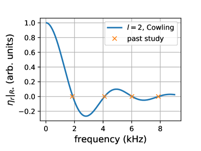
| From [136] (kHz) | 1.335 | 3.473 | 5.335 | 7.136 | 1.846 | 4.100 | 6.019 | 7.867 | 2.228 | 4.622 | 6.635 | 8.600 |
| From [157] (kHz) | - | - | - | - | 1.890 | 4.130 | - | - | - | - | - | - |
| Current work (kHz) | 1.376 | 3.469 | 5.336 | 7.141 | 1.881 | 4.104 | 6.028 | 7.866 | 2.255 | 4.640 | 6.647 | 8.535 |
| % diff. with [136] | 3.7 | 0.12 | 0.019 | 0.070 | 2.4 | 0.096 | 0.15 | 0.013 | 1.2 | 0.39 | 0.18 | 0.76 |
| % diff. with [157] | - | - | - | - | 0.48 | 0.63 | - | - | - | - | - | - |
Relative to the full Cowling approximation, the corrections obtained for the fundamental () mode frequencies for in [152] using the partially relaxed Cowling approximation are all upward, whereas the true frequencies have been found to be at lower values for a wide variety of modes and stars, eg. [137, 172, 173, 174, 175]. We also checked that this presumably erroneous upward correction for the fundamental modes occurs for as well. On the other hand, for all modes with that we checked for , the correction to the mode frequency supplied by the partial Cowling approximation is downward, as one would expect. This is shown for in Table (16.2), where the overtone frequencies are more correct than the fundamental ones, in comparison to the full Cowling approximation. The partial Cowling approximation also begins to fail to reproduce the correct number of nodes for modes with increasing and , and even to fail to reproduce modes at all (i.e. none satisfying the boundary condition at the surface of the star).
The erroneous upward correction of the fundamental mode frequencies in the partial Cowling approximation potentially calls into question the conclusion of [152] that the dominant gravitational wave emission is due to the fundamental (and ) mode, since that conclusion is based solely on the coincidence over time between that mode’s frequency (as computed in the partial Cowling approximation) and the peak emission in the gravitational wave spectrograms from simulations. A comparison between the perturbative eigenfunctions and the velocity data from simulations would conclusively identify the dominantly radiating mode. Hence we follow this eigenfunction-matching strategy in this work.
Our simulations extend only to ms after bounce, which is much shorter than the range of s considered in [152], so we cannot attempt to reproduce their mode identifications. However, rather than identify modes via coincident frequencies while ignoring the mode functions, we take the opposite approach by identifying modes via mode function matching while ignoring the mode frequencies. Given the errors introduced by the Cowling and partial Cowling approximations, as well as possible errors in the simulations arising from approximate treatments of the hydrodynamics and/or gravity, we advocate this approach since we believe it is less likely that these approximations would confuse modes at the level of the mode functions.
| From [156], GR CFC (kHz) | 1.586 | 3.726 | 2.440 | 4.896 |
| Current work, partial Cowling (kHz) | 2.496 | 3.777 | 3.047 | 4.999 |
| Current work, Cowling (kHz) | 1.881 | 4.104 | 2.565 | 5.112 |
| % diff. [156] vs partial Cowling | 57 | 1.4 | 25 | 2.1 |
| % diff. [156] vs Cowling | 19 | 10 | 5.1 | 4.4 |
16.5 TOV mode test in the FLASH implementation [94]
In this study we use the FLASH [158, 159] implementation of [94], which uses Newtonian hydrodynamics and a phenomenological effective gravitational potential developed in [160, 161, 93], designed to mimic general relativity in spherical symmetry. The neutrino physics is also implemented using the M1 scheme [162]. However, in this section we test only the Newtonian hydrodynamics and effective gravitational treatment in the context of the modes of oscillation of a stable TOV star. This test is particularly relevant to our study since we will be extracting the dominant modes of oscillation in core-collapse supernova simulations within this implementation.
A TOV migration test was carried out in [94], where a TOV star on the unstable branch is observed to migrate to the stable branch. The ensuing oscillations were observed to have a frequency higher than in the general relativistic case. In this section we extract the fundamental radial () and axisymmetric quadrupolar (, ) modes , and their overtones , , , , from the same stable TOV star studied in Secs. (13.2) (16.4) (central density , , ). To extract both radial and quadrupolar modes, we initialize the simulation with a velocity perturbation
| (16.16) |
(in units ), where is the radius of the star. This perturbation was used in [156] as a trial eigenfunction for the excitation of quadrupolar modes in rotating and non-rotating stars, but we find it also excites radial modes in our case. It comes from the vector spherical harmonic for , .
Mode identification proceeds via band-passing the velocity field around dominant frequency peaks in the simulations. The frequency peaks for the radial modes are identified from the central density evolution. Its average is subtracted and then the resulting time series is windowed using a Gaussian function, which enhances the peaks in the Fourier transform. The frequency peaks for the quadrupolar modes are instead extracted from the evolution of . We first subtract a Gaussian-smoothed version of itself to eliminate any secular variation, and the result is again windowed with a Gaussian and then its spectra are computed and averaged along a line with . These spectra are displayed in Fig. (16.2) (Left), with peaks labelled and indicated with vertical black solid lines.
After band-passing the velocity field about these frequency peaks, an angular decomposition into vector spherical harmonics is performed. This allows us to compute the total energy (integrated over time and space) in each poloidal number , i.e. the angular spectra of the frequency peaks. These spectra are displayed in Fig. (16.2) (Center), and serve to show the concentration of energy in for the radial modes and for the quadrupolar modes. A lone exception is the mode which we claim is the fundamental quadrupolar one, . It is contaminated by a strong part which appears nodeless. We verified that this frequency peak corresponds to a linear mode by increasing the perturbation strength by and observing the peak amplitude change linearly in response. However, the contamination did not disappear, and its energy scaled by the same factor as the part. This may have to do with the close proximity of the -mode frequency. Alternatively, it could mean that our FLASH implementation incorrectly reproduces the pure- character of mode functions of spherical stars. All the quadrupolar overtones, on the other hand, have dominant energy in .
The vector spherical harmonic decomposition also allows for the observation of the radial modefunction associated with a given and given frequency peak, and snapshots of these are displayed in Fig. (16.2). These radial mode functions reveal the node counts of the modes, which helps justify our mode identifications.

With the modes identified, the frequencies can now be compared with those obtained in the Cowling approximation and those obtained in full GR (in the conformal flatness approximation in the case of the non-radial modes). These comparisons are shown in Table (16.3). The mode frequencies extracted from the FLASH simulations are overestimated with respect to full GR in all cases. In comparison to the Cowling approximation, the FLASH simulations yield an improvement in the fundamental radial mode frequency (i.e. downward correction) only, but a worsening in the case of all other modes (i.e. upward correction).
These observations help to interpret the results of the current work, where we will be identifying the modes of oscillation in rotating CCSN simulations in FLASH with the expectation that the true frequencies are significantly lower than those observed in our simulations. We will see that the Cowling frequencies are lower than the simulation by a factor . As we saw in Sec. (11.2), the relativistic hydrodynamic fluxes contain factors of the lapse , which would serve to slow fluid motions inside a gravitational well. The FLASH implementation uses Newtonian hydrodynamics and therefore the lapse is absent. However, it seems that the overestimates of mode frequencies cannot be totally accounted for by the lapse, which only reaches a minimum of at the origin. This suggests the effective gravitational potential, also used in the FLASH implementation, is responsible for a large fraction of the error.
| From [156] & [137], GR CFC (kHz) | 1.442 | 3.955 | 5.916 | 1.586 | 3.726 | - | - |
| Current work, Cowling (kHz) | 2.696 | 4.534 | 6.346 | 1.881 | 4.104 | 6.028 | 7.866 |
| Current work, FLASH (kHz) | 2.174 | 5.522 | 8.295 | 2.024 | 5.122 | 7.920 | 10.593 |
| % diff. FLASH vs GR CFC | +51 | +40 | +40 | +28 | +37 | - | - |
| % diff. FLASH vs Cowling | -19 | +22 | +31 | +8 | +25 | +31 | +35 |
Chapter 17 Results & Discussion
17.1 , mode around Hz (Cowling)
In this section we implicate an , mode in producing prominent gravitational wave frequency peaks in all rad/s pre-collapse rotation cases, with coincident frequency peaks in the neutrino luminosities in a subset of cases. We will see that this mode picks up deformations consistent with expected leading order effects in rotation. The mode’s frequency in the simulation steadily rises across the sequence of rotating models, from Hz to Hz in the rad/s case where it is thoroughly mixed with many other and possibly other modes. The chief result will be the clean identification of peak frequencies of oscillation in gravitational waves and neutrino luminosities, both caused by the same mode whose frequency in the Cowling approximation is Hz, about lower than the simulation (and likely still overestimated).
17.1.1 rad/s model

This frequency band mask around Hz has most of its energy stored in between ms, with and containing second and third most energy (see Fig. (17.1) (Left)). We will argue that the component is its own mode, and that it is responsible for signal features in the rotating models as well as the non-rotating model. We will follow all the dominant modes in the band for as long as we can, and the will be followed across the entire sequence of models.
Firstly, we interpret these three dominant components as different modes based on a few known facts and observations which we already outlined in Secs. (15.1) and (16.3):
-
1.
Modes of spherical stars are pure spherical harmonics, so no mixing of ’s is expected. Although this simulation is not enforcing spherical symmetry exactly, the condition of zero rotation is enforced exactly, which means deformations of the proto-neutron star away from spherical are small. Thus, one does not expect any given mode to have -mixing so strong as to have comparable energy in different , as we observe in Fig. (17.1) (Left).
-
2.
The component is forbidden to be part of the or modes since it has odd parity in this non-rotating model (velocity has no part) whereas the components have even parity.
-
3.
The component, although having parity consistent with the component, does not manifest the same decay rate as the component in Fig. (17.1) (Left).
Next, we note that the gravitational wave emission observed within the band mask in Fig. (17.1) (Left) is certainly dominated by the component, since the gravitational wave signal itself was extracted using the quadrupole formula. Physically we expect this to be true as well, since the component has the most energy and is a vastly more efficient radiator of gravitational wave energy, being enhanced with respect to by a factor [176].
In Fig. (17.1) (Center & Right) we make direct comparisons between the velocity data and the perturbative mode functions computed at and ms on the CCSN background using the Cowling approximation. The first column compares the density-weighted radial mode functions , and the second column compares the non-radial functions . We observe a small change in both the perturbative and simulated mode functions between and ms, which illustrates the separation of scale between the oscillation period of the modes and the characteristic time over which the background changes. The inset zooms in on the low-energy region km to show any nodes which may be present there in the perturbative mode functions. In the case of the mode, we also display the velocity data smoothed using a Gaussian window of width km, since in this case the noise level is low enough to show a meaningful agreement with the perturbative mode function.
The mode displayed in Fig. (17.1) (Right) has , as compared with most other possibilities with , where the difference is defined in Eq. (16.15) and its surrounding discussion. We display the value of for all candidate modes for as a function of their frequencies in Fig. (17.2) (Left). The circles indicate the minima of , which occur for the best-fit modes.
In Fig. (17.2) (Right) we plot the node counts for all candidate modes as a function of their frequencies. The best-fit mode frequencies are indicated in vertical lines. Typically one expects -modes to have increasing frequency as increases, and the opposite behavior for -modes, with the fundamental mode living at the boundary of these two mode classes (see eg. [151, 153]). Since the best-fit modes occur near the boundary between these two behaviors in Fig. (17.2) (Right), we are unable to identify the modes as - or -modes on this basis.
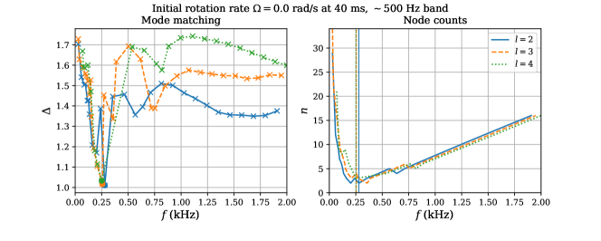
The best-matching perturbative mode at ms has a Cowling frequency of Hz, roughly lower than that observed in the simulation. We already showed in Sec. (16.5) that our FLASH implementation overestimates the frequencies of all modes with respect to the Cowling approximation (except the -mode). Furthermore, the Cowling approximation itself tends to overestimate the true frequency of modes. Thus, the Cowling value of Hz should be taken to be an upper bound on the true frequency of this mode. As discussed in Sec. (16.5), the lapse reaches a minimum value at the origin of , so its absence in the hydrodynamic equations does not completely account for the discrepancy. This suggests the effective gravitational potential accounts for a large fraction of it.
Neutrino emission for rad/s model
In Fig. (17.3) we display the sky-averaged neutrino lightcurves for the rad/s model (Left) along with the spherically-averaged neutrinosphere radii (Right, Top) and their spectra (Right, Bottom). The spectra are computed after subtracting a smoothing of , so as to accentuate any fluctuations about the mean that may be present. We observe no prominent frequency peak within the limits of the Hz band mask at ms (shown in black vertical lines).
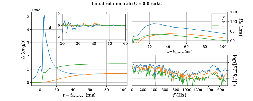
17.1.2 rad/s model

In the rad/s model, we have a slight change in the frequency mask as displayed in Fig. (17.4) (Left), but without well-separated energies between the different ’s. Nonetheless, comparison between the velocity data in the rad/s case and the perturbative mode functions from the rad/s case at ms still display good agreement.
In more detail: we begin with the mode function snapshots at ms from the rad/s model displayed in Fig. (17.1) (Centre & Right). For each band mask defined on the rad/s model, we do a search for the best-fit mode function snapshots for each of the modes separately, over a time interval of width ms centred on ms. This part of the search is required since there is no reason to expect the phase of each mode to remain the same across different rotation cases. Once the best-fit snapshots are found within each band mask, the best-fit across the band masks is computed, also using as described around Eq. (16.15). In this way, we obtain the band mask that is most likely to contain the mode, based on continuity of its mode function. We stress that this is done separately for each mode, since different mode frequencies will depend on differently and so there is no reason to expect them all to be contained in the same band mask as we move along the sequence of rotation models.
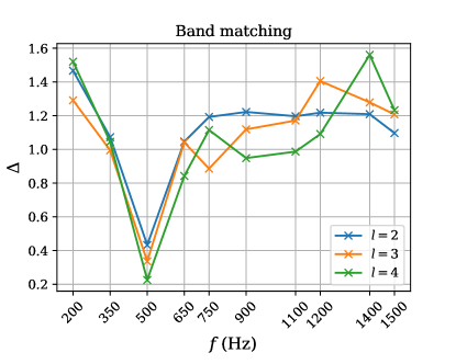
We display the best-fit values over the aforementioned time window for each band mask in the rad/s model in Fig. (17.5). Each tick label on the horizontal axis represents a band mask, and we see that is minimized distinctly for each of the modes at the Hz band mask. This means that each of those modes has happened to land in that mask for the rad/s model, although this was not guaranteed.
Neutrino emission for rad/s model
The neutrino luminosity spectrograms appear to have the beginnings of a frequency band coincident with the one currently under analysis. This will be more prominent in the next rotation rate of rad/s.
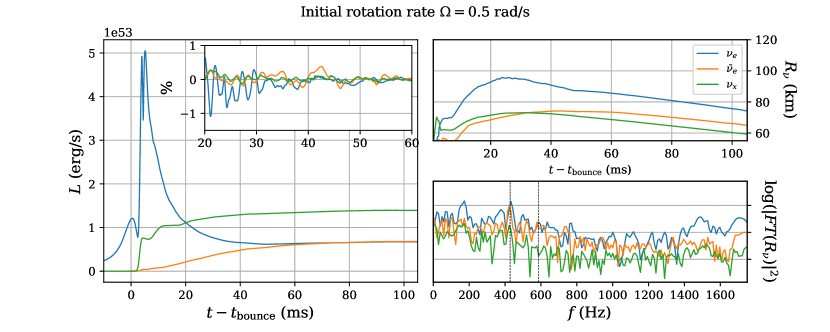
17.1.3 rad/s model
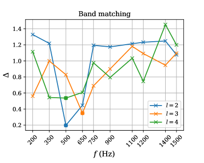
In Fig. (17.7) we display the band matching for the modes going from the rad/s models. The mode continues to be best-fit by the Hz band, whereas the mode has moved to the Hz band where it is a subdominant component. We thus stop following the mode. The mode has similar levels of fit between multiple bands, which signals that we have lost track of it. This occurs since, not only do modes deform as varies, but the excitation of them by the core bounce changes as well since the bounce proceeds differently. For example, the bounce occurs at the poles before the equator, and at different radii, since there is rotational support at the equator but not at the poles. This is at odds with the work of eg. [156] upon which our analysis is based, where the applied excitation of the star is under control and designed to excite specific modes. We thus also stop following the mode, and focus solely on the mode.

In the rad/s model, we continue to observe convincing continuity of the mode function in Fig. (17.8) (Right, Top Row). The frequency mask has shifted more than when going from rad/s, but it is still a modest shift with the masks overlapping in Fig. (17.8) (Left). At this rotation rate we observe a clear separation in the energy, energy, and the remaining poloidal numbers. We will now argue that the components are deformations of the mode we are following.
If the components are deformations of the mode, they must have the same (even) parity. Since are odd, only their components have even parity. We display the energy vs time in the components of in Fig. (17.8) (Center, Bottom), along with the components of (even parity) and component of (odd parity) for comparison. We observe that the even parity pieces have energies evolving with a unified exponential decay rate, whereas the odd parity , piece (which cannot be part of the mode) has noticeably different behaviour. Furthermore, since the band mask displayed in Fig. (17.8) (Left) has many frequency bins in it, one can check to see whether the even parity pieces () have the same frequency of oscillation as the even parity pieces (). This is confirmed, and displayed in Fig. (17.8) (Right, Bottom); we plot the frequency spectrum of the same energies, which without the smoothing performed in Fig. (17.8) (Center, Bottom) exhibit oscillations at twice the frequency of the underlying motion (and we compensate for this by rescaling the horizontal axis). We observe that the even parity parts of the components have peaks occurring at the same frequency (indicated with color-matching vertical lines). The odd parity , component, however, peaks Hz away.
Lastly, axial deformations () are the type of deformations of a polar () mode we would expect at first order in the rotation rate [155], as we described in Sec. (15.1). Rotational orders occur in powers of the ratio , where is the Keplerian orbital frequency . For the current model at ms, this ratio is when averaged over the inner km, where the bulk of the mode energy resides (see Fig. (17.8)). The energy ratio between the and parts of the mode at ms averages to a commensurate value, . These observations taken together tell us that we have correctly followed the mode from rad/s and that it has picked up axial deformations, and when following the mode further along our sequence of rotating models we will do the best-fit search according to snapshots of all the and components of the mode function.
The frequency mask is coincident with the peak gravitational wave emission, as seen in Fig. (17.8) (Left). It is also coincident with prominent frequency bands in the neutrino luminosity spectrograms, as we will describe next.
Neutrino emission for rad/s model
In Fig. (17.9) (Left) we plot the sky-averaged neutrino luminosities for electron neutrinos (blue), electron anti-neutrinos (orange), and the remaining flavours muon and tau are combined and denoted as (green). The muon and tau flavours are grouped together due to their similar behaviour at the typical energies of a CCSN system. Namely, their scattering cross-section with material in the system is significantly lower than for electron-flavour neutrinos since the muon and tau particles are too heavy to be produced in large numbers with the energy available.
The neutrino luminosities exhibit oscillatory behaviour, as shown in the inset of Fig. (17.9) (Left). There we have subtracted a Gaussian smoothing and normalized by the luminosity values at ms. The inset therefore displays the oscillations as a percentage of the luminosities. In Fig. (17.9) (Right, Top) we plot the spherically-averaged neutrinosphere radii vs time, defined as the radius at which the optical depth to infinity is . Roughly speaking, the stellar material is considered transparent to neutrinos outside of the neutrinosphere, although this is a heuristic notion because the transparency varies continuously and the neutrinosphere radius in fact depends on the energy of the neutrinos. Nonetheless, the neutrinosphere radius can be considered as tracking the the region producing free-streaming neutrinos. We see that the neutrinosphere radii also exhibit oscillations, and in Fig. (17.9) (Right, Bottom) we display Fourier spectra of them (with a Gaussian smoothing subtracted). Spectral peaks are seen within the range of frequencies covered by our Hz band mask, indicated in black dashed vertical lines. The coincidence in frequency between the neutrino luminosity oscillations, the neutrinosphere radii oscillations, and the mode under consideration suggest a cause for the former. Namely, that the , mode of the system is causing oscillations in the free-streaming neutrino emitting volume, which is impacting the neutrino lightcurves for an observer far away. If this is true, one expects an pattern of oscillatory emission on the sky, which we will show next.
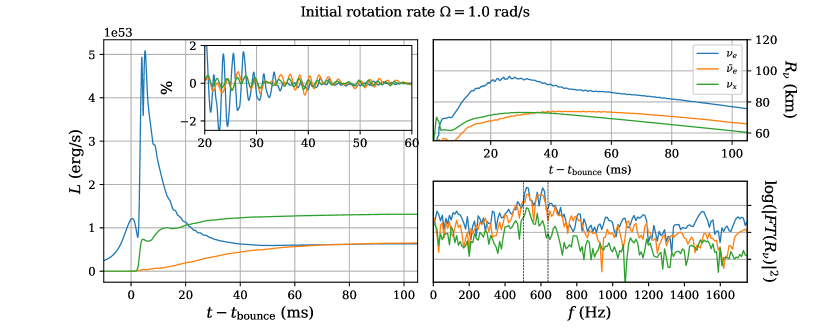
In Fig. (17.10) we display spectrograms of the neutrino luminosities with a smoothing subtracted (Top Row) for (Left), (Centre), and (Right), with the band mask of the mode overlaid. Also overlaid on the spectrograms are the spherical harmonic coefficients in absolute value for the neutrino luminosity pattern on the sky, Gaussian-smoothed in time with a ms window to eliminate oscillations. We observe that the emission pattern indeed has a strong component, along with a competing part. For comparison, we plot the energy in the radial part of the mode integrated over a km thick shell centred on the neutrinospheres (Bottom Row). We plot only the radial part since that is what would produce changes in the volume of the neutrino-emitting region. We see a similar level of excitation between the and components as in the neutrino emission pattern. This supports the notion that the mode we are following is producing an oscillatory variation in the neutrino-emitting volume, which then imprints on the neutrino lightcurves. We will also see that the mode in the next model in our sequence ( rad/s) has an deformation clearly identifiable at , which may explain the prevalence of the part in Fig. (17.10) in the outer km of the PNS where the neutrinosphere surfaces reside.
We have therefore implicated this mode as imprinting itself upon both the gravitational waves and the neutrino luminosities, producing peak oscillatory emission in both cases. The neutrinos carry information about the outer tails of the mode where km, whereas the gravitational waves probe the inner core.
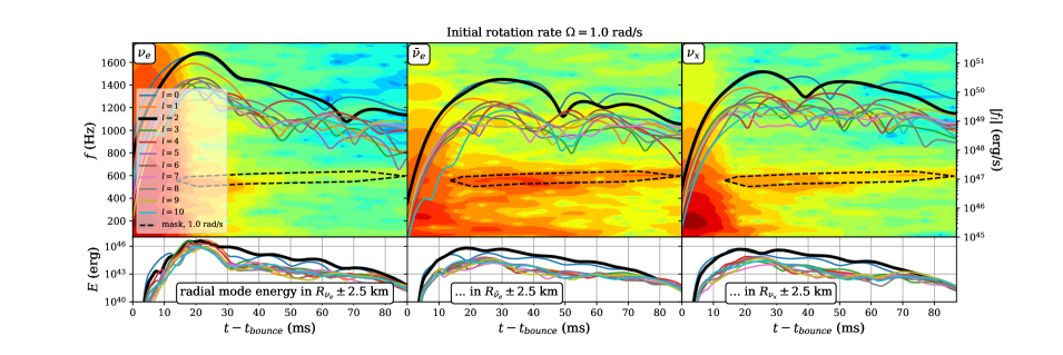
17.1.4 rad/s model
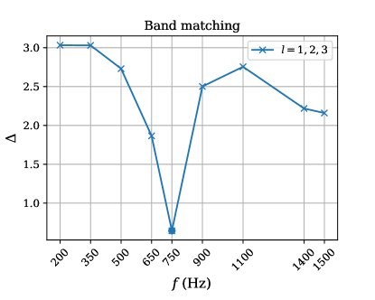
In Fig. (17.11) we display the band matching from rad/s models for the combination of the and parts, which to first-order in constitute the deformed mode that we are following. The mode has migrated from the Hz band to the Hz band, where is minimized distinctly.

In Fig. (17.12) (Left) we continue to see a similar distribution of energy as in the last rotation model, with dominant with deformations, and all other poloidal numbers subdominant. The current Hz mask continues to be coincident with an emission feature in the gravitational wave spectrogram, but the most dominant emission seems to occur at frequencies just below the mask. In Fig. (17.12) (Centre, Bottom) we again see the energies of the components of this deformed mode evolving in unison, as compared with the energy which is forbidden to be part of this mode by parity selection rules. As well we see again coincident frequency peaks in Fig. (17.12) (Right, Bottom), quite distinct from the spectrum. The average ratio of the and energies at ms has grown to , still commensurate with .
We even see evidence that an deformation has entered at . The peak frequency in Fig. (17.12) (Right, Bottom) is aligned with the rest of the components of the mode, and its energy evolution in Fig. (17.12) (Center, Bottom) is also commensurate. Furthermore, its energy at ms is of the energy in , which compares well with the expected order . Polar deformations such as this are expected at second order in rotation for the polar axisymmetric mode we are following [155]. The remaining poloidal numbers have energies about one order less than the energy at relative strength.
Neutrino emission for rad/s model
While the neutrino emission continues to exhibit oscillations in the rad/s model, it appears whiter in frequency than the rad/s model. This can be seen in the time domain in Fig. (17.13) (Left, Inset), and is also reflected in the frequency spectra of the neutrinosphere radii in (Right, Bottom). The Hz mask frequency bounds are again displayed in vertical black lines, where no remarkable peaks are apparent. Thus this mode does not appear to be coincident with a prominent modulation in the neutrino luminosities for this model.
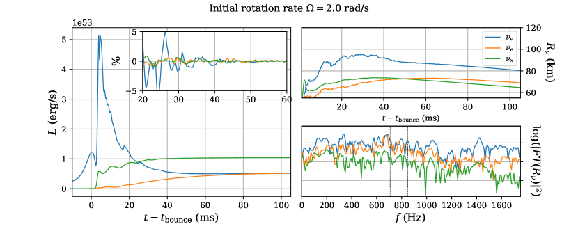
This is further demonstrated in Fig. (17.14), where the band mask does not surround any dominant emission, with the possible exception of . Nonetheless, the emission that does exist within the band mask still has a slight dominance in and (Top Row), in concert with the radial mode energy around the neutrinospheres (Bottom Row).
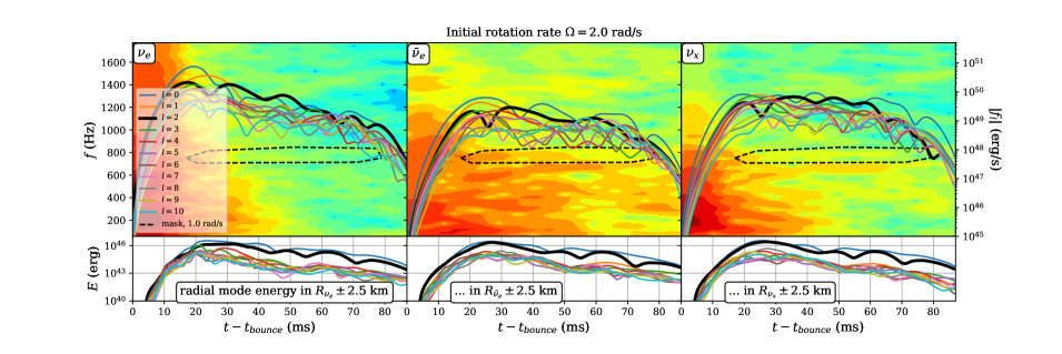
17.1.5 rad/s model
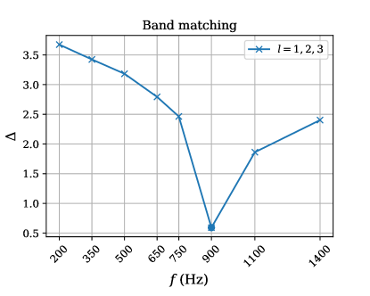
In Fig. (17.15) we continue to see this deformed mode migrate to higher frequencies, now falling within the Hz band for our most rapidly spinning rad/s model. However, as shown in Fig. (17.16) (Left), the energies in many different are becoming comparable. The ratio averaged over the inner km for this model is . We see in Fig. (17.16) (Centre, Bottom) that even the energy is evolving in unison with the mode we are following (although it cannot be part of the mode, by parity), and in Fig. (17.16) (Right, Bottom) we see the frequency peaks beginning to split apart.
Both of these facts are signalling that we are beginning to lose track of this mode, as other distinct oscillations are apparently excited as well. We interpret the unified evolution of the energy as arising from a common source, the strong rotational kinematics of the star. In order to separate the many modes that are present, one would need to do a perturbative calculation on this rapidly rotating background to obtain the mode functions, and do a large search for a best-fit combination of modes and amplitudes. This would be quite challenging, and is beyond our scope here.

Neutrino emission for rad/s model
The neutrino emission continues to have modulations with an incoherent appearance in time, and there are few if any distinguished peaks in the spectra of the neutrinosphere radii (see Fig. (17.17).
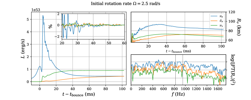
In Fig. (17.18) we see the Hz band mask for this model not enclosing anything remarkable in the neutrino spectrograms, with a partial exception for (Top Row). The emission pattern on the sky is well-mixed in (Top Row), and the radial mode energy around the neutrinosphere even more so (Bottom Row). Thus we cannot credibly claim any connection between the mode and the neutrino emission in this rapidly-rotating model.
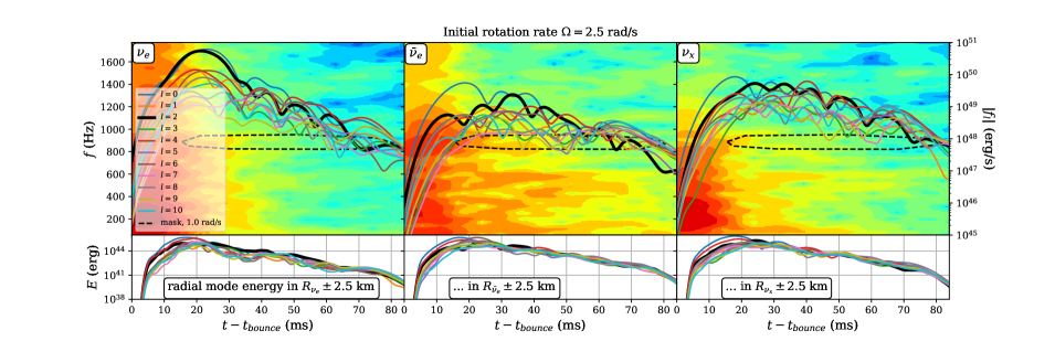
17.1.6 mode frequency for all models
Finally, we present the frequency of the mode, as extracted from the component, across all models in our sequence of rotating stars in Fig. (17.19). The ratio is computed at ms and averaged over the innermost km. The frequency of the mode decreases slightly from the rad/s model (first two points), and then rises monotonically along the sequence from the rad/s model onwards. The increase may be surprising, since the central density at ms decreases monotonically from across the rad/s models, and one expects mode frequencies to scale with (and therefore decrease) [155]. The opposite trend we see may be due to an additional limitation of our FLASH implementation to accurately reproduce mode frequencies of stars with rapid rotation.
We also plot a corrected version of the mode frequency trend in Fig. (17.19) (black), where we have multiplied all the frequencies by a factor , which is the correction required to scale the mode frequency in the non-rotating model to its best-fit Cowling value. We reiterate that the Cowling value is most likely an overestimate of the true frequency as well, as we saw in Sec. (16.4). Together with the a priori expectation that the mode frequency should be decreasing along a sequence of models with decreasing central density, one ought to regard the corrected curve in Fig. (17.19) as as upper bound on the true frequency for all models on the sequence.
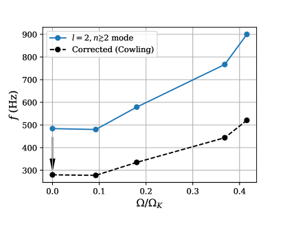
Chapter 18 Conclusion
In this part, we showed using a ZAMS model that detailed asteroseismology of the proto-neutron star at the centre of a rotating core-collapse supernovae is possible with both gravitational waves and neutrinos. These two messengers are complementary in that they carry information about certain linear modes of the core at different radii, with neutrinos probing the outer km and gravitational waves probing deeper in, km. The mechanism by which the linear modes of the core imprint themselves on the neutrino lightcurves appears to be that the neutrino-emitting volume undergoes deformations in time according to the frequency and angular harmonics of the modes in the vicinity of the neutrinospheres. The dominant angular harmonics are then reflected in the emission pattern of neutrinos on the sky.
As we saw in Chapter (17), many other spectral peaks exist both in gravitational wave and neutrino luminosity spectrograms along our entire sequence of rotating models. In Appendix (A) we show numerous additional modes matched between perturbation theory and our non-rotating model. The many modes that are active offer to explain the additional spectral peaks we observe along our rotating sequence.
We followed a strategy of mode function matching, rather than mode frequency matching as in [151, 152, 153]. This we believe is a more robust approach that is less susceptible to mode misidentification, especially given the approximations employed in both simulations and perturbative schemes. It is somewhat laborious work, but clearly a wealth of information can be extracted from any given model. A fully automated suite of algorithms would be desirable to hasten analysis and increase reproducibility.
Further investigation is necessary to fully understand the limitations of the FLASH implementation used in this work. We tested the accuracy of the implementation in reproducing modes of a non-rotating stable TOV star in Sec. (16.5) and found a systematic overestimation of the mode frequencies (except for the -mode). A question we were not able to answer is whether the modes (but particularly the -mode) are pure spherical harmonics. This can be answered by repeated rounds of mode recycling, which we have not done. Furthermore, the question of whether the FLASH implementation provides even lower quality of representation of mode frequencies for rapidly rotating stars we left completely open. However, we have some indication that the implementation performs poorly in this regime based on the trend of increasing frequency observed in Fig. (17.19), which is the opposite of what one would expect based on the decreasing central density of the proto-neutron star along the sequence of rotating models. Confirmation of this would require repeating a study such as [156] in our implementation, where the modes of stable rotating stars are extracted from nonlinear simulations with the aid of mode recycling. Confirming this would also bolster our tracking of the mode across the model sequence, since it would explain why the frequency would rise and by how much.
Appendix A Other modes in rad/s case
For the interested reader, in this appendix we show comparisons between the velocity data and perturbative mode functions for many other frequency bands we were able to identify. The purpose of this deluge of figures is to convey the following:
-
•
Identification of modes via a matching procedure between perturbative mode functions and velocity data from simulations is robust and repeatable, across a wide range of frequency spanning at least Hz.
-
•
The quality of a given mode match depends on its level of excitation, and the below figures have instances of very exceptional matches and rather poor ones. This is expected, since noise or nonlinear motion in the simulations would have a certain amplitude which the mode would need to rise above in order to be clearly identified. Thus the figures below should convey the range of quality of mode matches that can occur in a CCSN simulation.
-
•
The spectrograms in Fig. (III) have many additional features which we have not pinned on any mode. However, given our results, they very likely are due to other modes. The figures below show a wide range of possible candidates. In future work, we will repeat the analysis of Chapter (17) on the modes shown in the figures below, for the purpose of even more detailed asteroseismology.
-
•
For the mode we focused on in Chapter (17), we were not able to characterize it as a - or -mode (because its node count occurred so close to the boundary case). But in some instances below we can clearly characterize modes as -modes., particular towards the higher end of the frequency range we consider.
The figures below are of the same format as those presented (with more explanation) in Chapter (17), so we refer to that chapter as a prerequisite for understanding the ones below.
Hz band:

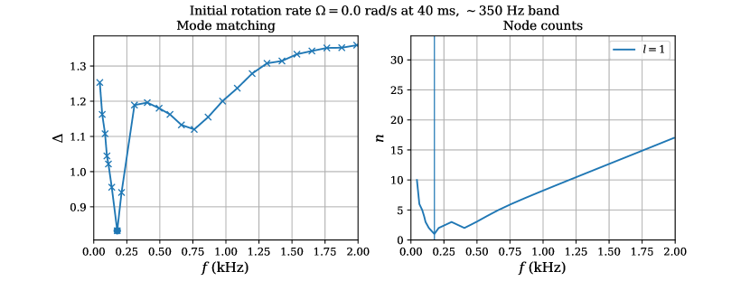
Hz band:

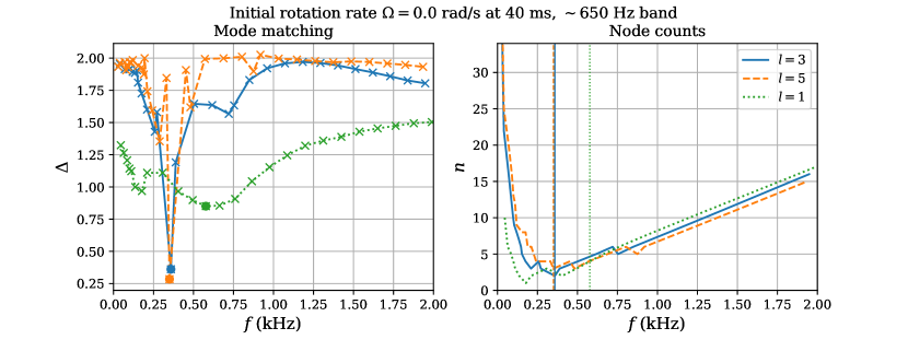
Hz band:

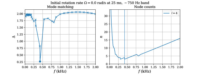
Hz band:

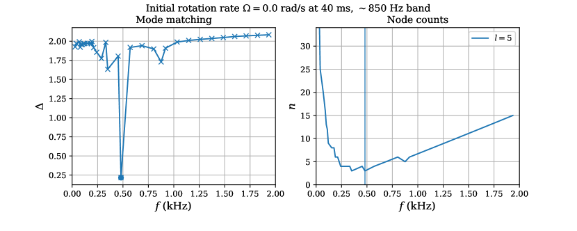
Hz band:

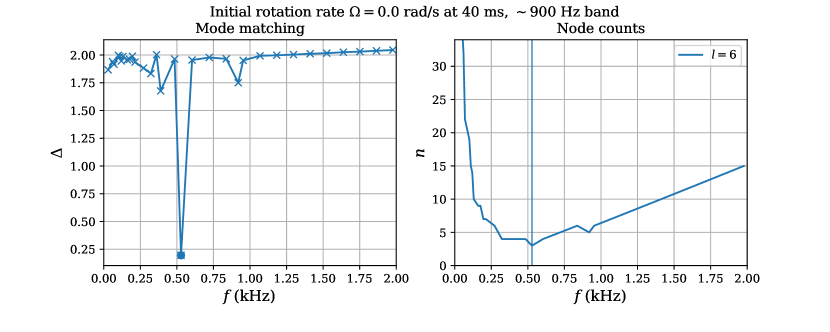
Hz band:

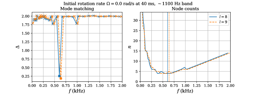
Hz band:

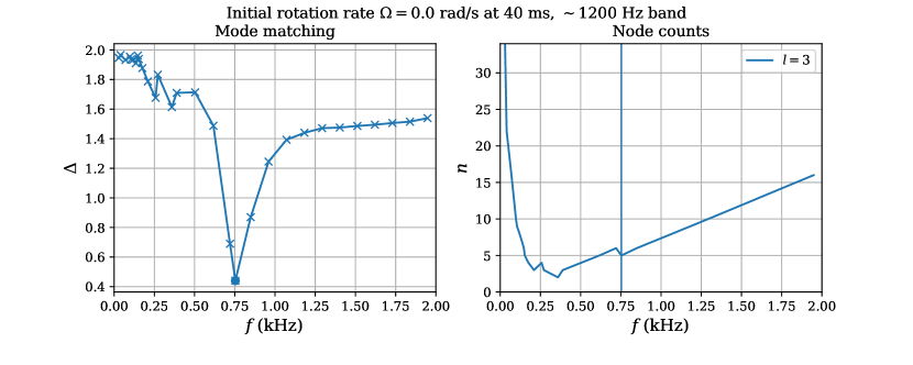
Hz band:

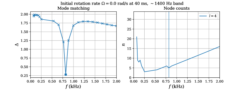
Hz band:

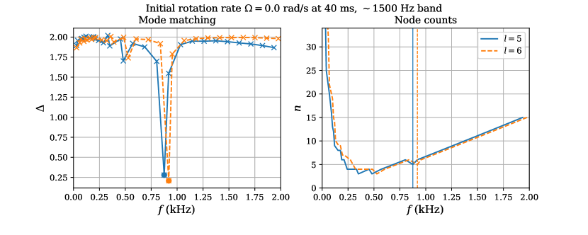
References
- Boffetta et al. [2000] G. Boffetta, A. Celani, and M. Vergassola, Phys. Rev. E 61, R29 (2000).
- Westernacher-Schneider et al. [2015] J. R. Westernacher-Schneider, L. Lehner, and Y. Oz, Journal of High Energy Physics 2015, 1 (2015).
- Rezzolla and Zanotti [2013] L. Rezzolla and O. Zanotti, Relativistic hydrodynamics (Oxford University Press, 2013).
- Gammie et al. [2003] C. F. Gammie, J. C. McKinney, and G. Toth, Astrophys. J. 589, 444 (2003), arXiv:astro-ph/0301509 [astro-ph] .
- Shibata and Sekiguchi [2005] M. Shibata and Y.-i. Sekiguchi, Phys. Rev. D72, 044014 (2005), arXiv:astro-ph/0507383 [astro-ph] .
- Baumgarte and Shapiro [2010] T. W. Baumgarte and S. L. Shapiro, Numerical Relativity: Solving Einstein’s Equations on the Computer (Cambridge University Press, New York, NY, USA, 2010).
- Lehner and Pretorius [2014] L. Lehner and F. Pretorius, Ann. Rev. Astron. Astrophys. 52, 661 (2014), arXiv:1405.4840 [astro-ph.HE] .
- Luzum and Romatschke [2008] M. Luzum and P. Romatschke, Phys. Rev. C78, 034915 (2008), [Erratum: Phys. Rev.C79,039903(2009)], arXiv:0804.4015 [nucl-th] .
- van der Schee et al. [2013] W. van der Schee, P. Romatschke, and S. Pratt, Phys. Rev. Lett. 111, 222302 (2013), arXiv:1307.2539 [nucl-th] .
- Baier et al. [2008] R. Baier, P. Romatschke, D. T. Son, A. O. Starinets, and M. A. Stephanov, JHEP 0804, 100 (2008), arXiv:0712.2451 [hep-th] .
- Bhattacharyya et al. [2008a] S. Bhattacharyya, V. E. Hubeny, S. Minwalla, and M. Rangamani, JHEP 0802, 045 (2008a), arXiv:0712.2456 [hep-th] .
- Eling et al. [2010] C. Eling, I. Fouxon, and Y. Oz, (2010), arXiv:1004.2632 [hep-th] .
- Carrasco et al. [2012] F. Carrasco, L. Lehner, R. C. Myers, O. Reula, and A. Singh, Phys. Rev. D86, 126006 (2012), arXiv:1210.6702 [hep-th] .
- Chesler and Yaffe [2013] P. M. Chesler and L. G. Yaffe, (2013), arXiv:1309.1439 [hep-th] .
- Galtier and Nazarenko [2017] S. Galtier and S. V. Nazarenko, (2017), arXiv:1703.09069 [gr-qc] .
- [16] J. Cayuso, N. Ortiz, and L. Lehner, To be submitted.
- R. Benzi and Chavarria [1995] C. B. R. Benzi, S. Ciliberto and G. R. Chavarria, Physica D 80, 385 (1995).
- Frisch [1996] U. Frisch, Turbulence, by Uriel Frisch, pp. 310. ISBN 0521457130. Cambridge, UK: Cambridge University Press, January 1996. 1 (1996).
- Dobler et al. [2003] W. Dobler, N. E. L. Haugen, T. A. Yousef, and A. Brandenburg, Physical Review E 68, 026304 (2003).
- Boffetta and Ecke [2012] G. Boffetta and R. E. Ecke, Annual Review of Fluid Mechanics 44, 427 (2012), http://www.annualreviews.org/doi/pdf/10.1146/annurev-fluid-120710-101240 .
- Cardy et al. [2008] J. Cardy, G. Falkovich, K. Gawedzki, S. Nazarenko, and O. Zaboronski, Non-equilibrium Statistical Mechanics and Turbulence, London Mathematical Society Le (Cambridge University Press, 2008).
- Fouxon and Oz [2010] I. Fouxon and Y. Oz, Phys. Lett. B694, 261 (2010), arXiv:0909.3574 [hep-th] .
- Eyink and Drivas [2017] G. L. Eyink and T. D. Drivas, ArXiv e-prints (2017), arXiv:1704.03541 [physics.flu-dyn] .
- Radice and Rezzolla [2013] D. Radice and L. Rezzolla, Astrophys. J. 766, L10 (2013), arXiv:1209.2936 [astro-ph.HE] .
- Green et al. [2014] S. R. Green, F. Carrasco, and L. Lehner, Phys. Rev. X4, 011001 (2014), arXiv:1309.7940 [hep-th] .
- Chandra et al. [2015] M. Chandra, C. F. Gammie, F. Foucart, and E. Quataert, Astrophys. J. 810, 162 (2015), arXiv:1508.00878 [astro-ph.HE] .
- Zrake and MacFadyen [2012] J. Zrake and A. I. MacFadyen, Astrophysical Journal 744, 32 (2012), arXiv:1108.1991 [astro-ph.HE] .
- Zrake and MacFadyen [2013] J. Zrake and A. I. MacFadyen, Astrophysical Journal Letters 763, L12 (2013), arXiv:1210.4066 [astro-ph.HE] .
- Zrake and East [2016] J. Zrake and W. E. East, The Astrophysical Journal 817, 89 (2016).
- Zhdankin et al. [2017] V. Zhdankin, G. R. Werner, D. A. Uzdensky, and M. C. Begelman, Phys. Rev. Lett. 118, 055103 (2017).
- Uzdensky [2017] D. A. Uzdensky, ArXiv e-prints (2017), arXiv:1703.04688 [astro-ph.HE] .
- Romatschke and Romatschke [2007] P. Romatschke and U. Romatschke, Phys. Rev. Lett. 99, 172301 (2007), arXiv:0706.1522 [nucl-th] .
- Heinz et al. [2012] U. Heinz, C. Shen, and H. Song, Proceedings, 19th International Conference on Particles and Nuclei (PANIC 11): Cambridge, USA, July 24-29, 2011, AIP Conf. Proc. 1441, 766 (2012), arXiv:1108.5323 [nucl-th] .
- Fukushima [2017] K. Fukushima, Rept. Prog. Phys. 80, 022301 (2017), arXiv:1603.02340 [nucl-th] .
- Bernard [1999] D. Bernard, Phys. Rev. E 60, 6184 (1999).
- Landau and Lifshitz [1987] L. D. Landau and E. M. Lifshitz, Fluid Mechanics (Butterworth-Heinemann, Oxford, UK, 1987).
- Honeycutt [1992] R. L. Honeycutt, Phys. Rev. A 45, 600 (1992).
- [38] “Intel mkl vector statistical library,” https://software.intel.com/en-us/node/521842, accessed: 2016-10-03.
- Mertens [2009] S. Mertens, ArXiv e-prints (2009), arXiv:0905.4238 [cond-mat.stat-mech] .
- Kraichnan [1967] R. H. Kraichnan, Physics of Fluids 10, 1417 (1967).
- Novikov [1965] E. Novikov, Sov. Phys. JETP 20, 1290 (1965).
- Gustafsson et al. [1995] B. Gustafsson, H. Kreiss, and J. Oliger, Time Dependent Problems and Difference Methods, A Wiley-Interscience Publication (Wiley, 1995).
- Courant et al. [1928] R. Courant, K. Friedrichs, and H. Lewy, Mathematische annalen 100, 32 (1928).
- Pasquero and Falkovich [2002] C. Pasquero and G. Falkovich, Phys. Rev. E 65, 056305 (2002).
- Chen et al. [2003] S. Chen, R. E. Ecke, G. L. Eyink, X. Wang, and Z. Xiao, Phys. Rev. Lett. 91, 214501 (2003).
- Borue [1994] V. Borue, Phys. Rev. Lett. 72, 1475 (1994).
- Kritsuk et al. [2007] A. G. Kritsuk, M. L. Norman, P. Padoan, and R. Wagner, The Astrophysical Journal 665, 416 (2007).
- Federrath [2013] C. Federrath, MNRAS 436, 1245 (2013), arXiv:1306.3989 [astro-ph.SR] .
- Falkovich [1994] G. Falkovich, Physics of Fluids 6, 1411 (1994).
- Biskamp et al. [1998] D. Biskamp, E. Schwarz, and A. Celani, Physical Review Letters 81, 4855 (1998).
- Scott [2007] R. K. Scott, Phys. Rev. E 75, 046301 (2007).
- Passot et al. [1995] T. Passot, E. Vazquez-Semadeni, and A. Pouquet, Astrophysical Journal 455, 536 (1995), astro-ph/9601182 .
- Chertkov et al. [2007] M. Chertkov, C. Connaughton, I. Kolokolov, and V. Lebedev, Phys. Rev. Lett. 99, 084501 (2007).
- Lindborg and Alvelius [2000] E. Lindborg and K. Alvelius, Physics of Fluids 12, 945 (2000), http://dx.doi.org/10.1063/1.870379 .
- Vallgren and Lindborg [2011] A. Vallgren and E. Lindborg, Journal of Fluid Mechanics 671, 168–183 (2011).
- Adams et al. [2014a] A. Adams, P. M. Chesler, and H. Liu, Phys. Rev. Lett. 112, 151602 (2014a), arXiv:1307.7267 [hep-th] .
- Bhattacharyya et al. [2009] S. Bhattacharyya, S. Minwalla, and S. R. Wadia, Journal of High Energy Physics 2009, 059 (2009).
- Fouxon and Oz [2008] I. Fouxon and Y. Oz, Phys. Rev. Lett. 101, 261602 (2008).
- Bhattacharyya et al. [2008b] S. Bhattacharyya, R. Loganayagam, I. Mandal, S. Minwalla, and A. Sharma, JHEP 0812, 116 (2008b), arXiv:0809.4272 [hep-th] .
- Van Raamsdonk [2008] M. Van Raamsdonk, JHEP 0805, 106 (2008), arXiv:0802.3224 [hep-th] .
- Hubeny et al. [2012] V. E. Hubeny, S. Minwalla, and M. Rangamani, in Black holes in higher dimensions (2012) pp. 348–383, [,817(2011)], arXiv:1107.5780 [hep-th] .
- Oz and Rabinovich [2011] Y. Oz and M. Rabinovich, JHEP 1102, 070 (2011), arXiv:1011.5895 [hep-th] .
- Eling and Oz [2013] C. Eling and Y. Oz, JHEP 1311, 079 (2013), arXiv:1308.1651 [hep-th] .
- Adams et al. [2012] A. Adams, P. M. Chesler, and H. Liu, (2012), arXiv:1212.0281 [hep-th] .
- Adams et al. [2014b] A. Adams, N. Benjamin, A. Moghaddam, and W. Musial, arXiv preprint arXiv:1411.2001 (2014b).
- Eling and Oz [2015] C. Eling and Y. Oz, JHEP 09, 150 (2015), arXiv:1502.03069 [nlin.CD] .
- Westernacher-Schneider and Lehner [2017] J. R. Westernacher-Schneider and L. Lehner, Journal of High Energy Physics 2017, 27 (2017).
- Yang et al. [2015] H. Yang, A. Zimmerman, and L. Lehner, Phys. Rev. Lett. 114, 081101 (2015), arXiv:1402.4859 [gr-qc] .
- Falconer [1986] K. J. Falconer, The geometry of fractal sets, Vol. 85 (Cambridge university press, 1986).
- Fontane et al. [2013] J. Fontane, D. G. Dritschel, and R. K. Scott, Physics of Fluids 25, 015101 (2013).
- Mandelbrot [1967] B. B. Mandelbrot, science 156, 636 (1967).
- Gneiting et al. [2012] T. Gneiting, H. Ševčíková, and D. B. Percival, Statistical Science , 247 (2012).
- Voss [1986] R. F. Voss, Physica Scripta 1986, 27 (1986).
- Barnsley [2014] M. F. Barnsley, Fractals everywhere (Academic press, 2014).
- Falconer [2004] K. Falconer, Fractal geometry: mathematical foundations and applications (John Wiley & Sons, 2004).
- Ott et al. [1984] E. Ott, W. Withers, and J. Yorke, Journal of Statistical Physics 36, 687 (1984).
- Turcotte [1997] D. L. Turcotte, Fractals and chaos in geology and geophysics (Cambridge university press, 1997).
- Cornish [1996] N. J. Cornish, arXiv preprint gr-qc/9602054 (1996).
- Cornish and Levin [1996] N. J. Cornish and J. J. Levin, Physical Review D 53, 3022 (1996).
- Cornish and Levin [1997] N. J. Cornish and J. J. Levin, Physical Review D 55, 7489 (1997).
- Frolov and Larsen [1999] A. V. Frolov and A. L. Larsen, Classical and Quantum Gravity 16, 3717 (1999).
- Lehner and Pretorius [2011] L. Lehner and F. Pretorius, arXiv preprint arXiv:1106.5184 (2011).
- Nollert and Herold [1996] H.-P. Nollert and H. Herold, in Relativity and Scientific Computing (Springer, 1996) pp. 330–351.
- Barausse and Lehner [2013] E. Barausse and L. Lehner, Physical Review D 88, 024029 (2013).
- Ott [2009] C. D. Ott, Classical and Quantum Gravity 26, 063001 (2009).
- Kotake [2013] K. Kotake, Comptes Rendus Physique 14, 318 (2013).
- Hills [1988] J. G. Hills, Nature 331, 687 (1988).
- Rees [1988] M. J. Rees, Nature 333, 523 (1988).
- Evans and Kochanek [1989] C. R. Evans and C. S. Kochanek, The Astrophysical Journal 346, L13 (1989).
- Dolence et al. [2015] J. C. Dolence, A. Burrows, and W. Zhang, The Astrophysical Journal 800, 10 (2015).
- Pan et al. [2016] K.-C. Pan, M. Liebendörfer, M. Hempel, and F.-K. Thielemann, The Astrophysical Journal 817, 72 (2016).
- Suwa et al. [2015] Y. Suwa, S. Yamada, T. Takiwaki, and K. Kotake, The Astrophysical Journal 816, 43 (2015).
- Marek et al. [2006] A. Marek, H. Dimmelmeier, H.-T. Janka, E. Müller, and R. Buras, Astronomy & Astrophysics 445, 273 (2006).
- O’Connor and Couch [2018] E. P. O’Connor and S. M. Couch, The Astrophysical Journal 854, 63 (2018).
- Paczynsky and Wiita [1980] B. Paczynsky and P. J. Wiita, Astronomy and Astrophysics 88, 23 (1980).
- Semerák and Karas [1999] O. Semerák and V. Karas, arXiv preprint astro-ph/9901289 (1999).
- Wegg [2012] C. Wegg, The Astrophysical Journal 749, 183 (2012).
- Tejeda and Rosswog [2013] E. Tejeda and S. Rosswog, Monthly Notices of the Royal Astronomical Society 433, 1930 (2013).
- Tejeda et al. [2017] E. Tejeda, E. Gafton, S. Rosswog, and J. C. Miller, Monthly Notices of the Royal Astronomical Society 469, 4483 (2017).
- Cheng and Evans [2013] R. M. Cheng and C. R. Evans, Physical Review D 87, 104010 (2013).
- Cheng and Bogdanović [2014] R. M. Cheng and T. Bogdanović, Physical Review D 90, 064020 (2014).
- East and Pretorius [2013] W. E. East and F. Pretorius, Physical Review D 87, 101502 (2013).
- East [2014] W. E. East, The Astrophysical Journal 795, 135 (2014).
- MacLeod et al. [2016] M. MacLeod, J. Guillochon, E. Ramirez-Ruiz, D. Kasen, and S. Rosswog, The Astrophysical Journal 819, 3 (2016).
- Kawana et al. [2018] K. Kawana, A. Tanikawa, and N. Yoshida, Monthly Notices of the Royal Astronomical Society 477, 3449 (2018).
- Tanikawa [2018] A. Tanikawa, The Astrophysical Journal 858, 26 (2018).
- Blanchet et al. [1990] L. Blanchet, T. Damour, and G. Schäefer, Monthly Notices of the Royal Astronomical Society 242, 289 (1990).
- Ayal et al. [2001] S. Ayal, T. Piran, R. Oechslin, M. Davies, and S. Rosswog, The Astrophysical Journal 550, 846 (2001).
- Ayal et al. [2000] S. Ayal, M. Livio, and T. Piran, The Astrophysical Journal 545, 772 (2000).
- Hayasaki et al. [2016] K. Hayasaki, N. Stone, and A. Loeb, Monthly Notices of the Royal Astronomical Society 461, 3760 (2016).
- Martí et al. [1991] J. M. Martí, J. M. Ibánez, and J. A. Miralles, Physical Review D 43, 3794 (1991).
- Alcubierre [2008] M. Alcubierre, Introduction to 3+1 Numerical Relativity, International Series of Monographs on Physics (OUP Oxford, 2008).
- Donat et al. [1998] R. Donat, J. A. Font, J. M. Ibánez, and A. Marquina, Journal of Computational Physics 146, 58 (1998).
- Ibáñez et al. [2001] J. M. Ibáñez, M. Aloy, J. Font, J. M. Martí, J. Miralles, and J. Pons, in Godunov Methods (Springer, 2001) pp. 485–496.
- Anderson and York Jr [1999] A. Anderson and J. W. York Jr, Physical Review Letters 82, 4384 (1999).
- Calabrese et al. [2002] G. Calabrese, L. Lehner, and M. Tiglio, Phys.Rev. D65, 104031 (2002), arXiv:gr-qc/0111003 [gr-qc] .
- LeVeque [1990] R. J. LeVeque, in Numerical Methods for Conservation Laws (Springer, 1990) pp. 122–135.
- LeVeque [2002] R. J. LeVeque, Finite volume methods for hyperbolic problems, Vol. 31 (Cambridge university press, 2002).
- Martí and Müller [2003] J. M. Martí and E. Müller, Living Reviews in Relativity 6, 7 (2003).
- Font [2008] J. A. Font, Living reviews in relativity 11, 7 (2008).
- Evans [1986] C. R. Evans, Dynamical spacetimes and numerical relativity , 3 (1986).
- Harten et al. [1983] A. Harten, P. D. Lax, and B. v. Leer, SIAM review 25, 35 (1983).
- Einfeldt [1988] B. Einfeldt, SIAM Journal on Numerical Analysis 25, 294 (1988).
- Colella and Woodward [1984] P. Colella and P. R. Woodward, Journal of Computational Physics 54, 174 (1984).
- Mignone et al. [2005] A. Mignone, T. Plewa, and G. Bodo, The Astrophysical Journal Supplement Series 160, 199 (2005).
- Laney [1998] C. B. Laney, Computational gasdynamics (Cambridge university press, 1998).
- Van Leer [1997] B. Van Leer, Journal of Computational Physics 135, 229 (1997).
- Galeazzi et al. [2013] F. Galeazzi, W. Kastaun, L. Rezzolla, and J. A. Font, Physical Review D 88, 064009 (2013).
- Petzold [1983] L. Petzold, SIAM journal on scientific and statistical computing 4, 136 (1983).
- Hindmarsh [1983] A. C. Hindmarsh, Scientific computing , 55 (1983).
- Jones et al. [01 ] E. Jones, T. Oliphant, P. Peterson, et al., “SciPy: Open source scientific tools for Python,” (2001–), [Online; accessed ¡today¿].
- Shu and Osher [1988] C.-W. Shu and S. Osher, Journal of computational physics 77, 439 (1988).
- Anderson et al. [2008] M. Anderson, E. W. Hirschmann, L. Lehner, S. L. Liebling, P. M. Motl, D. Neilsen, C. Palenzuela, and J. E. Tohline, Physical Review D 77, 024006 (2008).
- Calabrese et al. [2004] G. Calabrese, L. Lehner, O. Reula, O. Sarbach, and M. Tiglio, Class. Quant. Grav. 21, 5735 (2004), arXiv:gr-qc/0308007 [gr-qc] .
- Hilborn et al. [2000] R. C. Hilborn et al., Chaos and nonlinear dynamics: an introduction for scientists and engineers (Oxford University Press on Demand, 2000).
- Font et al. [2001] J. A. Font, H. Dimmelmeier, A. Gupta, and N. Stergioulas, Monthly Notices of the Royal Astronomical Society 325, 1463 (2001).
- Font et al. [2002] J. A. Font, T. Goodale, S. Iyer, M. Miller, L. Rezzolla, E. Seidel, N. Stergioulas, W.-M. Suen, and M. Tobias, Physical Review D 65, 084024 (2002).
- Baiotti et al. [2010] L. Baiotti, I. Hawke, P. J. Montero, and L. Rezzolla, arXiv preprint arXiv:1004.3849 (2010).
- Radice and Rezzolla [2011] D. Radice and L. Rezzolla, Physical Review D 84, 024010 (2011).
- Yoshida and Eriguchi [2001] S. Yoshida and Y. Eriguchi, Monthly Notices of the Royal Astronomical Society 322, 389 (2001).
- Kastaun [2006] W. Kastaun, Physical Review D 74, 124024 (2006).
- Schoepe et al. [2017] A. Schoepe, D. Hilditch, and M. Bugner, arXiv preprint arXiv:1712.09837 (2017).
- Agrež [2007] D. Agrež, IEEE Trans. Instrum. Meas 56, 2111 (2007).
- Hergt and Schäfer [2008] S. Hergt and G. Schäfer, Physical Review D 77, 104001 (2008).
- Neilsen [1999] D. W. Neilsen, Extremely Relativistic Fluids in Strong-Field Gravity, Ph.D. thesis, University of Texas at Austin (1999).
- Hirata et al. [1987] K. Hirata, T. Kajita, M. Koshiba, M. Nakahata, Y. Oyama, N. Sato, A. Suzuki, M. Takita, Y. Totsuka, T. Kifune, et al., Physical Review Letters 58, 1490 (1987).
- Bionta et al. [1991] R. Bionta, G. Blewitt, C. Bratton, D. Casper, A. Ciocio, R. Claus, B. Cortez, M. Crouch, S. Dye, S. Errede, et al., in Neutrinos And Other Matters: Selected Works of Frederick Reines (World Scientific, 1991) pp. 340–342.
- Ott et al. [2012] C. Ott, E. Abdikamalov, E. O’Connor, C. Reisswig, R. Haas, P. Kalmus, S. Drasco, A. Burrows, and E. Schnetter, Physical Review D 86, 024026 (2012).
- Kuroda et al. [2017] T. Kuroda, K. Kotake, K. Hayama, and T. Takiwaki, The Astrophysical Journal 851, 62 (2017).
- Fuller et al. [2015] J. Fuller, H. Klion, E. Abdikamalov, and C. D. Ott, Monthly Notices of the Royal Astronomical Society 450, 414 (2015).
- Torres-Forné et al. [2017] A. Torres-Forné, P. Cerdá-Durán, A. Passamonti, and J. A. Font, Monthly Notices of the Royal Astronomical Society 474, 5272 (2017).
- Morozova et al. [2018] V. Morozova, D. Radice, A. Burrows, and D. Vartanyan, arXiv preprint arXiv:1801.01914 (2018).
- Torres-Forné et al. [2018] A. Torres-Forné, P. Cerdá-Durán, A. Passamonti, M. Obergaulinger, and J. A. Font, arXiv preprint arXiv:1806.11366 (2018).
- Pan et al. [2018] K.-C. Pan, M. Liebendörfer, S. M. Couch, and F.-K. Thielemann, The Astrophysical Journal 857, 13 (2018).
- Friedman and Stergioulas [2013] J. L. Friedman and N. Stergioulas, Rotating relativistic stars (Cambridge University Press, 2013).
- Dimmelmeier et al. [2006] H. Dimmelmeier, N. Stergioulas, and J. A. Font, Monthly Notices of the Royal Astronomical Society 368, 1609 (2006).
- Gaertig and Kokkotas [2008] E. Gaertig and K. D. Kokkotas, Physical Review D 78, 064063 (2008).
- Fryxell et al. [2000] B. Fryxell, K. Olson, P. Ricker, F. Timmes, M. Zingale, D. Lamb, P. MacNeice, R. Rosner, J. Truran, and H. Tufo, The Astrophysical Journal Supplement Series 131, 273 (2000).
- Dubey et al. [2009] A. Dubey, K. Antypas, M. K. Ganapathy, L. B. Reid, K. Riley, D. Sheeler, A. Siegel, and K. Weide, Parallel Computing 35, 512 (2009).
- Keil [1997] W. Keil, PhD thesis, Technische Universitaet Muenchen, Munich, Germany, (1997) (1997).
- Rampp and Janka [2002] M. Rampp and H.-T. Janka, Astronomy & Astrophysics 396, 361 (2002).
- O’Connor [2015] E. O’Connor, The Astrophysical Journal Supplement Series 219, 24 (2015).
- Thorne [1980] K. S. Thorne, Reviews of Modern Physics 52, 299 (1980).
- Reisswig et al. [2011] C. Reisswig, C. D. Ott, U. Sperhake, and E. Schnetter, Physical Review D 83, 064008 (2011).
- Woosley and Heger [2007] S. Woosley and A. Heger, Physics Reports 442, 269 (2007).
- Steiner et al. [2013] A. W. Steiner, M. Hempel, and T. Fischer, The Astrophysical Journal 774, 17 (2013).
- Zwerger and Mueller [1997] T. Zwerger and E. Mueller, Astronomy and Astrophysics 320, 209 (1997).
- Ott et al. [2004] C. D. Ott, A. Burrows, E. Livne, and R. Walder, The Astrophysical Journal 600, 834 (2004).
- Tassoul [2015] J.-L. Tassoul, Theory of Rotating Stars.(PSA-1), Vol. 1 (Princeton University Press, 2015).
- Reisenegger and Goldreich [1992] A. Reisenegger and P. Goldreich, The Astrophysical Journal 395, 240 (1992).
- Takiwaki et al. [2012] T. Takiwaki, K. Kotake, and Y. Suwa, The Astrophysical Journal 749, 98 (2012).
- Cerdá-Durán et al. [2008] P. Cerdá-Durán, J. A. Font, L. Antón, and E. Müller, Astronomy & Astrophysics 492, 937 (2008).
- Zink et al. [2010] B. Zink, O. Korobkin, E. Schnetter, and N. Stergioulas, Physical Review D 81, 084055 (2010).
- Chirenti et al. [2015] C. Chirenti, G. H. de Souza, and W. Kastaun, Physical Review D 91, 044034 (2015).
- Mendes and Ortiz [2018] R. F. Mendes and N. Ortiz, Physical Review Letters 120, 201104 (2018).
- Thorne [1969] K. S. Thorne, The astrophysical journal 158, 997 (1969).