Deep learning with differential Gaussian process flows

Abstract

We propose a novel deep learning paradigm of differential flows that learn a stochastic differential equation transformations of inputs prior to a standard classification or regression function. The key property of differential Gaussian processes is the warping of inputs through infinitely deep, but infinitesimal, differential fields, that generalise discrete layers into a dynamical system. We demonstrate state-of-the-art results that exceed the performance of deep Gaussian processes and neural networks.

1 INTRODUCTION

Gaussian processes are a family of flexible kernel function distributions (Rasmussen and Williams, 2006). The capacity of kernel models is inherently determined by the function space induced by the choice of the kernel, where standard stationary kernels lead to models that underperform in practice. Shallow – or single – Gaussian processes are often suboptimal since flexible kernels that would account for the non-stationary and long-range connections of the data are difficult to design and infer. Such models have been proposed by introducing non-stationary kernels (Tolvanen et al., 2014; Heinonen et al., 2016), kernel compositions (Duvenaud et al., 2011; Sun et al., 2018), spectral kernels (Wilson et al., 2013; Remes et al., 2017), or by applying input-warpings (Snoek et al., 2014) or output-warpings (Snelson et al., 2004; Lázaro-Gredilla, 2012). Recently, Wilson et al. (2016) proposed to transform the inputs with a neural network prior to a Gaussian process model. The new neural input representation can extract high-level patterns and features, however, it employs rich neural networks that require careful design and optimization.

Deep Gaussian processes elevate the performance of Gaussian processes by mapping the inputs through multiple Gaussian process ’layers’ (Damianou and Lawrence, 2013; Salimbeni and Deisenroth, 2017), or as a network of GP nodes (Duvenaud et al., 2011; Wilson et al., 2012; Sun et al., 2018). However, deep GP’s result in degenerate models if the individual GP’s are not invertible, which limits their capacity (Duvenaud et al., 2014).

In this paper we propose a novel paradigm of learning continuous-time transformations or flows of the data instead of learning a discrete sequence of layers. We apply stochastic differential equation systems in the original data space to transform the inputs before a classification or regression layer. The transformation flow consists of an infinite path of infinitesimal steps. This approach turns the focus from learning iterative function mappings to learning input representations in the original feature space, avoiding learning new feature spaces.

Our experiments show state-of-the-art prediction performance on a number of benchmark datasets on classification and regression. The performance of the proposed model exceeds that of competing Bayesian approaches, including deep Gaussian processes.

2 BACKGROUND

We begin by summarising useful background of Gaussian processes and continuous-time dynamicals models.

2.1 Gaussian processes

Gaussian processes (GP) are a family of Bayesian models that characterise distributions of functions (Rasmussen and Williams, 2006). A Gaussian process prior on a function $f(\mathbf{x})$ over vector inputs $\mathbf{x}\in\mathbb{R}^{D}$,

$$f(\mathbf{x}) \sim\mathcal{GP}(0,K(\mathbf{x},\mathbf{x}^{\prime})),$$ (1)

defines a prior distribution over function values $f(\mathbf{x})$ whose mean and covariances are

$$\mathbb{E}[f(\mathbf{x})] =0$$ (2)

$$\operatorname{\textbf{cov}}[f(\mathbf{x}),f(\mathbf{x}^{\prime})] =K(\mathbf{x},\mathbf{x}^{\prime}).$$ (3)

A GP prior defines that for any collection of $N$ inputs, $\mathbf{X}=(\mathbf{x}_{1},\ldots,\mathbf{x}_{N})^{T}$, the corresponding function values $\mathbf{f}=(f(\mathbf{x}_{1}),\ldots,f(\mathbf{x}_{N}))^{T}\in\mathbb{R}^{N}$ are coupled to following the multivariate normal distribution

$$\mathbf{f}\sim\mathcal{N}(\mathbf{0},\mathbf{K}),$$ (4)

where $\mathbf{K}=(K(\mathbf{x}_{i},\mathbf{x}_{j}))_{i,j=1}^{N}\in\mathbb{R}^{N\times N}$ is the kernel matrix. The key property of GP’s is that output predictions $f(\mathbf{x})$ and $f(\mathbf{x}^{\prime})$ correlate depending on how similar are their inputs $\mathbf{x}$ and $\mathbf{x}^{\prime}$, as measured by the kernel $K(\mathbf{x},\mathbf{x}^{\prime})\in\mathbb{R}$.

We consider sparse Gaussian process functions by augmenting the Gaussian process with a small number $M$ of inducing ‘landmark’ variables $u=f(\mathbf{z})$ (Snelson and Ghahramani, 2006). We condition the GP prior with the inducing variables $\mathbf{u}=(u_{1},\ldots,u_{M})^{T}\in\mathbb{R}^{M}$ and $\mathbf{Z}=(\mathbf{z}_{1},\ldots,\mathbf{z}_{M})^{T}$ to obtain the GP posterior predictions at data points

$$\mathbf{f}|\mathbf{u};\mathbf{Z} \sim\mathcal{N}(\mathbf{Q}\mathbf{u},\mathbf{K}_{\mathbf{X}\mathbf{X}}-\mathbf{Q}\mathbf{K}_{\mathbf{Z}\mathbf{Z}}\mathbf{Q}^{T})$$ (5)

$$\mathbf{u} \sim\mathcal{N}(\mathbf{0},\mathbf{K}_{\mathbf{Z}\mathbf{Z}}),$$ (6)

where $\mathbf{Q}=\mathbf{K}_{\mathbf{X}\mathbf{Z}}\mathbf{K}_{\mathbf{Z}\mathbf{Z}}^{-1}$, and where $\mathbf{K}_{\mathbf{X}\mathbf{X}}\in\mathbb{R}^{N\times N}$ is the kernel between observed image pairs $\mathbf{X}\times\mathbf{X}$, the kernel $\mathbf{K}_{\mathbf{X}\mathbf{Z}}\in\mathbb{R}^{N\times M}$ is between observed images $\mathbf{X}$ and inducing images $\mathbf{Z}$, and kernel $\mathbf{K}_{\mathbf{Z}\mathbf{Z}}\in\mathbb{R}^{M\times M}$ is between inducing images $\mathbf{Z}\times\mathbf{Z}$. The inference problem of sparse Gaussian processes is to learn the parameters $\theta$ of the kernel (such as the lengthscale), and the conditioning inducing variables $\mathbf{u},\mathbf{Z}$.

2.2 Stochastic differential equations

Stochastic differential equations (SDEs) are an effective formalism for modelling continuous-time systems with underlying stochastic dynamics, with wide range of applications (Friedrich et al., 2011). We consider multivariate continuous-time systems governed by a Markov process $\mathbf{x}_{t}$ described by SDE dynamics

$$d\mathbf{x}_{t}={\boldsymbol{\mu}}(\mathbf{x}_{t})dt+\sqrt{{\boldsymbol{\Sigma}}(\mathbf{x}_{t})}dW_{t},$$ (7)

where $\mathbf{x}_{t}\in\mathbb{R}^{D}$ is the state vector of a $D$-dimensional dynamical system at continuous time $t\in\mathbb{R}$, ${\boldsymbol{\mu}}(\mathbf{x}_{t})\in\mathbb{R}^{D}$ is a deterministic state evolution vector field, $\sqrt{\Sigma(\mathbf{x}_{t})}\in\mathbb{R}^{D\times D}$ is the diffusion matrix field of the stochastic multivariate Wiener process $W_{t}\in\mathbb{R}^{D}$. The $\sqrt{\Sigma(\mathbf{x}_{t})}$ is the square root matrix of a covariance matrix $\Sigma(\mathbf{x}_{t})$, where we assume $\Sigma(\mathbf{x}_{t})=\sqrt{\Sigma(\mathbf{x}_{t})}\sqrt{\Sigma(\mathbf{x}_{t})}$ holds. A Wiener process has zero initial state $W_{0}=\mathbf{0}$, and independent, Gaussian increments $W_{t+s}-W_{t}\sim\mathcal{N}(\mathbf{0},sI_{D})$ over time with standard deviation $\sqrt{s}I_{D}$ (See Figure 1).

Figure 1: An example vector field defined by the inducing vectors (a) results in the ODE flow solutions (b) of a 2D system. Including the colored Wiener diffusion (c) leads to SDE trajectory distributions (d).

(a) Sparse GP

(b) Deep GP

(c) Differentially deep GP

Figure 2: The sparse Gaussian processes uncouples the observations through global inducing variables $\mathbf{u}_{g}$ (a). Deep Gaussian process is a hierarchical model with a nested composition of Gaussian processes introducing layer dependency. Layer-specific inducing variables $\mathbf{u}_{g}^{(\ell)}$ introduce conditional independence between function values $\mathbf{g}_{i}^{(\ell)}$ within each layer (b). In our formulation deepness is introduced as a temporal dependency across states $\mathbf{x}_{i}(t)$ (indicated by dashed line) with a GP prior over their differential function value $\mathbf{f}_{i}$ (c). Global inducing variables ${\mathbf{u}_{\mathbf{f}}}$ can be used to introduce conditional independence between differential function values at a particular time point.

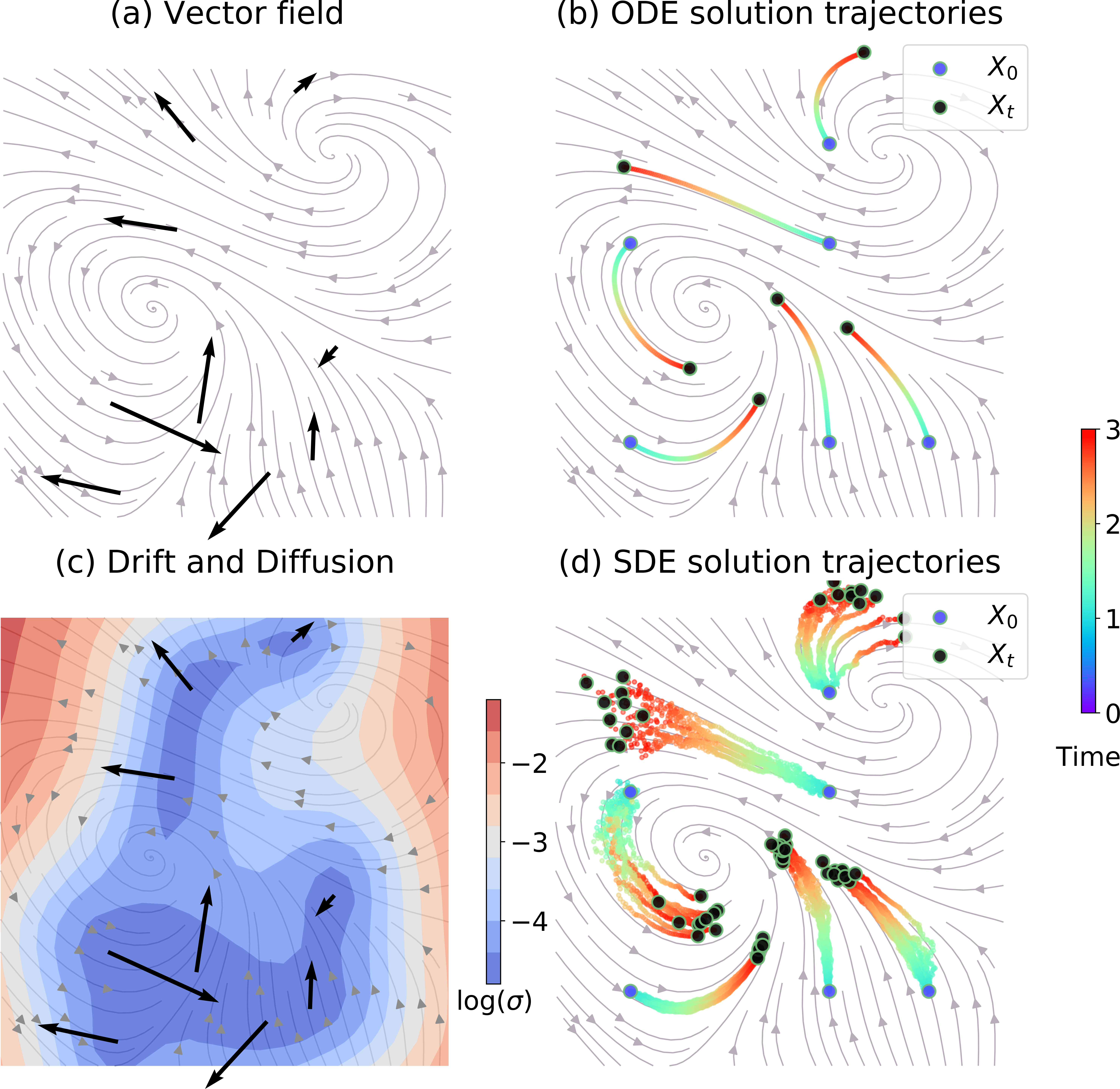
The SDE system (7) transforms states $\mathbf{x}_{t}$ forward in continuous time by the deterministic drift function ${\boldsymbol{\mu}}:\mathbb{R}^{D}\rightarrow\mathbb{R}^{D}$, while the diffusion ${\boldsymbol{\Sigma}}:\mathbb{R}^{D}\rightarrow\mathbb{R}^{D\times D}$ is the scale of the random Brownian motion $W_{t}$ that scatter the state $\mathbf{x}_{t}$ with random fluctuations. The state solutions of an SDE are given by the stochastic Itô integral (Oksendal, 2014)

$$\mathbf{x}_{t} =\mathbf{x}_{0}+\int_{0}^{t}{\boldsymbol{\mu}}(\mathbf{x}_{\tau})d\tau+\int_{0}^{t}\sqrt{{\boldsymbol{\Sigma}}(\mathbf{x}_{\tau})}dW_{\tau},$$ (8)

where we integrate the system state from an initial state $\mathbf{x}_{0}$ for time $t$ forward, and where $\tau$ is an auxiliary time variable. SDEs produce continuous, but non-smooth trajectories $\mathbf{x}_{0:t}$ over time due to the non-differentiable Brownian motion. This causes the SDE system to not have a time derivative $\frac{d\mathbf{x}_{t}}{dt}$, but the stochastic Itô integral (8) can still be defined.

The only non-deterministic part of the solution (8) is the Brownian motion $W_{\tau}$, whose random realisations generate path realisations $\mathbf{x}_{0:t}$ that induce state distributions

$$\mathbf{x}_{t}\sim p_{t}(\mathbf{x};{\boldsymbol{\mu}},{\boldsymbol{\Sigma}},\mathbf{x}_{0})$$ (9)

at any instant $t$, given the drift ${\boldsymbol{\mu}}$ and diffusion ${\boldsymbol{\Sigma}}$ from initial state $\mathbf{x}_{0}$. The state distribution is the solution to the Fokker-Planck-Kolmogorov (FPK) partial differential equation, which is intractable for general non-linear drift and diffusion.

In practise the Euler-Maruyama (EM) numerical solver can be used to simulate trajectory samples from the state distribution (Yildiz et al., 2018) (See Figure 1d). We assume a fixed time discretisation $t_{1},\ldots,t_{N}$ with $\Delta t=t_{N}/N$ being the time window (Higham, 2001). The EM method at $t_{k}$ is

$$\mathbf{x}_{k+1} =\mathbf{x}_{k}+{\boldsymbol{\mu}}(\mathbf{x}_{k})\Delta t+\sqrt{\Sigma(\mathbf{x}_{k})}\Delta W_{k},$$ (10)

where $\Delta W_{k}=W_{k+1}-W_{k}\sim\mathcal{N}(\mathbf{0},\Delta tI_{D})$ with standard deviation $\sqrt{\Delta t}$. The EM increments $\Delta\mathbf{x}_{k}=\mathbf{x}_{k+1}-\mathbf{x}_{k}$ correspond to samples from a Gaussian

$$\Delta\mathbf{x}_{k}\sim\mathcal{N}({\boldsymbol{\mu}}(\mathbf{x}_{k})\Delta t,\Sigma(\mathbf{x}_{k})\Delta t).$$ (11)

Then, the full $N$ length path is determined from the $N$ realisations of the Wiener process, each of which is a $D$-dimensional. More efficient high-order approximations have also been developed (Kloeden and Platen, 1992; Lamba et al., 2006).

SDE systems are often constructed by manually defining drift and diffusion functions to model specific systems in finance, biology, physics or in other domains (Friedrich et al., 2011). Recently, several works have proposed learning arbitrary drift and diffusion functions from data (Papaspiliopoulos et al., 2012; García et al., 2017; Yildiz et al., 2018).

3 DEEP DIFFERENTIAL GAUSSIAN PROCESS

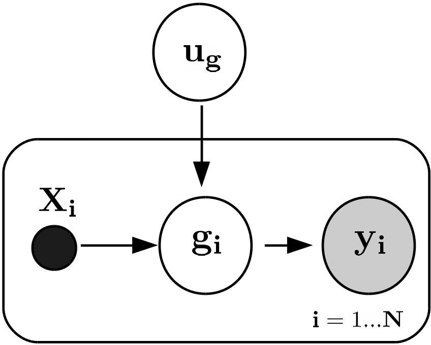
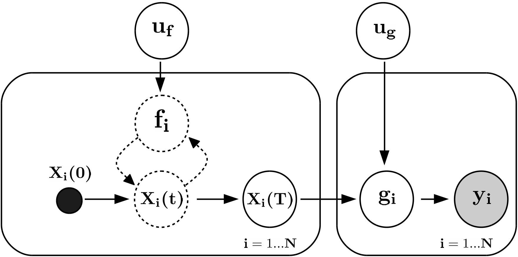
In this paper we propose a paradigm of continuous-time deep learning, where inputs $\mathbf{x}_{i}$ are not treated as constant, but are instead driven by an SDE system. We propose a continuous-time deep Gaussian process model through infinite, infinitesimal differential compositions, denoted as DiffGP. In DiffGP, a Gaussian process warps or flows an input $\mathbf{x}$ through an SDE system until a predefined time $T$, resulting in $\mathbf{x}(T)$, which is subsequently classified or regressed with a separate function. We apply the process to both train and test inputs. We impose GP priors on both the stochastic differential fields and the predictor function (See Figure 2). A key parameter of the differential GP model is the amount of simulation time $T$, which defines the length of flow and the capacity of the system, analogously to the number of layers in standard deep GPs or deep neural networks.

We assume a dataset of $N$ inputs $\mathbf{X}=(\mathbf{x}_{1},\ldots,\mathbf{x}_{N})^{T}\in\mathbb{R}^{N\times D}$ of $D$-dimensional vectors $\mathbf{x}_{i}\in\mathbb{R}^{D}$, and associated scalar outputs $\mathbf{y}=(y_{1},\ldots,y_{N})^{T}\in\mathbb{R}^{N}$ that can be continuous for a regression problem or categorical for classification, respectively. We redefine the inputs as temporal functions $\mathbf{x}:\mathcal{T}\rightarrow\mathbb{R}^{D}$ over time such that state paths $\mathbf{x}_{t}$ over time $t\in\mathcal{T}=\mathbb{R}_{+}$ emerge, where the observed inputs $\mathbf{x}_{i,t}\triangleq\mathbf{x}_{i,0}$ correspond to initial states $\mathbf{x}_{i,0}$ at time $0$. We classify or regress the final data points $\mathbf{X}_{T}=(\mathbf{x}_{1,T},\ldots,\mathbf{x}_{N,T})^{T}$ after $T$ time of an SDE flow with a predictor Gaussian process

$$g(\mathbf{x}_{T}) \sim\mathcal{GP}(0,K(\mathbf{x}_{T},\mathbf{x}^{\prime}_{T}))$$ (12)

to classify or regress the outputs $\mathbf{y}$. The framework reduces to a conventional Gaussian process with zero flow time $T=0$ (See Figure 2).

The prediction depends on the final dataset $\mathbf{X}_{T}$ structure, determined by the SDE flow $d\mathbf{x}_{t}$ from the original data $\mathbf{X}$. We consider SDE flows of type

$$d\mathbf{x}_{t}={\boldsymbol{\mu}}(\mathbf{x}_{t})dt+\sqrt{\Sigma(\mathbf{x}_{t})}dW_{t}$$ (13)

where

$${\boldsymbol{\mu}}(\mathbf{x}) =\mathbf{K}_{\mathbf{x}{\mathbf{Z}_{\mathbf{f}}}}\mathbf{K}_{{\mathbf{Z}_{\mathbf{f}}}{\mathbf{Z}_{\mathbf{f}}}}^{-1}\mathrm{vec}({\mathbf{U}_{\mathbf{f}}})$$ (14)

$${\boldsymbol{\Sigma}}(\mathbf{x}) =\mathbf{K}_{\mathbf{x}\mathbf{x}}-\mathbf{K}_{\mathbf{x}{\mathbf{Z}_{\mathbf{f}}}}\mathbf{K}_{{\mathbf{Z}_{\mathbf{f}}}{\mathbf{Z}_{\mathbf{f}}}}^{-1}\mathbf{K}_{{\mathbf{Z}_{\mathbf{f}}}\mathbf{x}}$$ (15)

are the vector-valued Gaussian process posteriors conditioned on equalities between $\mathbf{f}(\mathbf{z})$, inducing vectors ${\mathbf{U}_{\mathbf{f}}}=(\mathbf{u}_{1}^{f},\ldots,\mathbf{u}_{M}^{f})^{T}$ and inducing states ${\mathbf{Z}_{\mathbf{f}}}=(\mathbf{z}_{1}^{f},\ldots,\mathbf{z}_{M}^{f})$. These choices of drift and diffusion correspond to an underlying GP

$$\mathbf{f}(\mathbf{x}) \sim\mathcal{GP}(\mathbf{0},K(\mathbf{x},\mathbf{x}^{\prime}))$$ (16)

$$\mathbf{f}(\mathbf{x})|{\mathbf{U}_{\mathbf{f}}},{\mathbf{Z}_{\mathbf{f}}} \sim\mathcal{N}({\boldsymbol{\mu}}(\mathbf{x}),{\boldsymbol{\Sigma}}(\mathbf{x}))$$ (17)

where $K(\mathbf{x},\mathbf{x}^{\prime})\in\mathbb{R}^{D\times D}$ is a matrix-valued kernel of the vector field $\mathbf{f}(\mathbf{x})\in\mathbb{R}^{D}$, and $\mathbf{K}_{{\mathbf{Z}_{\mathbf{f}}}{\mathbf{Z}_{\mathbf{f}}}}=(K(\mathbf{z}_{i}^{f},\mathbf{z}_{j}^{f}))_{i,j=1}^{M}\in\mathbb{R}^{MD\times MD}$ block matrix of matrix-valued kernels (similarly for $\mathbf{K}_{\mathbf{x}{\mathbf{Z}_{\mathbf{f}}}}$).

The vector field $\mathbf{f}(\mathbf{x})$ is now a GP with deterministic conditional mean ${\boldsymbol{\mu}}$ and covariance ${\boldsymbol{\Sigma}}$ at every location $\mathbf{x}$ given the inducing variables. We encode the underlying GP field mean and covariance uncertainty into the drift and diffusion of the SDE flow (13). The Wiener process $W_{t}$ of an SDE samples a new fluctuation from the covariance ${\boldsymbol{\Sigma}}$ around the mean ${\boldsymbol{\mu}}$ at every instant $t$. This corresponds to an affine transformation

$$(\mathbf{f}(\mathbf{x})-{\boldsymbol{\mu}}(\mathbf{x}))\sqrt{\Delta t}+{\boldsymbol{\mu}}(\mathbf{x})\Delta t \sim\mathcal{N}({\boldsymbol{\mu}}(\mathbf{x})\Delta t,\Sigma(\mathbf{x})\Delta t),$$ (18)

which shows that samples from the vector field GP match the SDE Euler-Maruyama increment $\Delta\mathbf{x}_{k}$ distribution (11). The state distribution $p_{T}(\mathbf{x};{\boldsymbol{\mu}},{\boldsymbol{\Sigma}},\mathbf{x}_{0})$ can then be represented as $p(\mathbf{x}_{T}|{\mathbf{U}_{\mathbf{f}}})=\int p(\mathbf{x}_{T}|\mathbf{f})p(\mathbf{f}|{\mathbf{U}_{\mathbf{f}}})d\mathbf{f}$ where $p(\mathbf{x}_{T}|\mathbf{f})$ is an Dirac distribution of the end point of a single Euler-Maruyama simulated path, and where the vector field $p(\mathbf{f})$ is marginalized along the Euler-Maruyama path.

Our model corresponds closely to the doubly-stochastic deep GP, where the Wiener process was replaced by random draws from the GP posterior $\varepsilon^{l}\cdot\Sigma^{l}(\mathbf{f}^{l-1})$ per layer $l$ (Salimbeni and Deisenroth, 2017). In our approach the continuous time $t$ corresponds to continuously indexed states, effectively allowing infinite layers that are infinitesimal.

3.1 Spatio-temporal fields

Earlier we assumed a global, time-independent vector field $\mathbf{f}(\mathbf{x}_{t})$, which in the standard models would correspond to a single ‘layer’ applied recurrently over time $t$. To extend the model capacity, we consider spatio-temporal vector fields $\mathbf{f}_{t}(\mathbf{x}):=\mathbf{f}(\mathbf{x},t)$ that themselves evolve as a function of time, effectively applying a smoothly changing vector field ‘layer’ at every instant $t$. We select a separable spatio-temporal kernel $K((\mathbf{x},t),(\mathbf{x}^{\prime},t^{\prime}))=K(\mathbf{x},\mathbf{x}^{\prime})k(t,t^{\prime})$ that leads to an efficient Kronecker-factorised (Stegle et al., 2011) spatio-temporal SDE flow

$$\mathbf{f}_{t}(\mathbf{x})|({\mathbf{Z}_{\mathbf{f}}^{s}},{\mathbf{Z}_{\mathbf{f}}^{t}},{\mathbf{U}_{\mathbf{f}}}) \sim\mathcal{N}({\boldsymbol{\mu}}_{t}(\mathbf{x}),{\boldsymbol{\Sigma}}_{t}(\mathbf{x}))$$ (19)

$${\boldsymbol{\mu}}_{t}(\mathbf{x}) =\mathbf{C}_{\mathbf{x}{\mathbf{Z}_{\mathbf{f}}}}\mathbf{C}_{{\mathbf{Z}_{\mathbf{f}}}{\mathbf{Z}_{\mathbf{f}}}}^{-1}\mathrm{vec}({\mathbf{U}_{\mathbf{f}}})$$ (20)

$${\boldsymbol{\Sigma}}_{t}(\mathbf{x}) =\mathbf{C}_{\mathbf{x}\mathbf{x}}-\mathbf{C}_{\mathbf{x}{\mathbf{Z}_{\mathbf{f}}}}\mathbf{C}_{{\mathbf{Z}_{\mathbf{f}}}{\mathbf{Z}_{\mathbf{f}}}}^{-1}\mathbf{C}_{{\mathbf{Z}_{\mathbf{f}}}\mathbf{x}},$$ (21)

where $\mathbf{C}_{\mathbf{x}\mathbf{x}}=K_{\mathbf{x}\mathbf{x}}k_{tt}$, $\mathbf{C}_{\mathbf{x}\mathbf{Z}}=\mathbf{K}_{\mathbf{x}{\mathbf{Z}_{\mathbf{f}}^{s}}}\otimes\mathbf{K}_{t{\mathbf{Z}_{\mathbf{f}}^{t}}}$ and $\mathbf{C}_{{\mathbf{Z}_{\mathbf{f}}}{\mathbf{Z}_{\mathbf{f}}}}=\mathbf{K}_{{\mathbf{Z}_{\mathbf{f}}^{s}}{\mathbf{Z}_{\mathbf{f}}^{s}}}\otimes\mathbf{K}_{{\mathbf{Z}_{\mathbf{f}}^{t}}{\mathbf{Z}_{\mathbf{f}}^{t}}}$, and where the spatial inducing states are denoted by ${\mathbf{Z}_{\mathbf{f}}^{s}}$ and the temporal inducing times by ${\mathbf{Z}_{\mathbf{f}}^{t}}$. In practice we place usually only a few (e.g. 3) temporal inducing times equidistantly on the range $[0,T]$. This allows the vector field itself to curve smoothly throughout the SDE. We only have a single inducing matrix ${\mathbf{U}_{\mathbf{f}}}$ for both spatial and temporal dimensions.

Figure 3: (a)Illustration of samples from a 2D deep Gaussian processes prior. DGP prior exhibits a pathology wherein representations in deeper layers concentrate on low-rank manifolds.(b) Samples from a differentially deep Gaussian processes prior result in rank-preserving representations.(c) The continuous-time nature of the warping trajectories results from smooth drift and structured diffusion (d).

3.2 Stochastic variational inference

The differential Gaussian process is a combination of a conventional prediction GP $g(\cdot)$ with an SDE flow GP $\mathbf{f}(\cdot)$ fully parameterised by $\mathbf{Z},\mathbf{U}$ as well as kernel parameters $\theta$. We turn to variational inference to estimate posterior approximations $q({\mathbf{U}_{\mathbf{f}}})$ and $q(\mathbf{u}_{g})$ for both models.

We start by augmenting the predictor function $g$ with $M$ inducing locations ${\mathbf{Z}_{g}}=(\mathbf{z}_{g1},\ldots,\mathbf{z}_{gM})$ with associated inducing function values $g(\mathbf{z})=u$ in a vector ${\mathbf{u}_{g}}=(u_{g1},\ldots,u_{gM})^{T}\in\mathbb{R}^{M}$. We aim to learn the distribution of the inducing values $\mathbf{u}$, while learning point estimates of the inducing locations $\mathbf{Z}$, which we hence omit from the notation below. The prediction conditional distribution is (Titsias, 2009)

$$p({\mathbf{g}}|{\mathbf{u}_{g}},{\mathbf{X}_{T}}) =\mathcal{N}({\mathbf{g}}|\mathbf{Q}_{T}{\mathbf{u}_{g}},\mathbf{K}_{{\mathbf{X}_{T}}{\mathbf{X}_{T}}}-\mathbf{Q}_{T}\mathbf{K}_{{\mathbf{Z}_{g}}{\mathbf{Z}_{g}}}\mathbf{Q}_{T}^{T})$$ (22)

$$p({\mathbf{u}_{g}}) =\mathcal{N}({\mathbf{u}_{g}}|\mathbf{0},\mathbf{K}_{{\mathbf{Z}_{g}}{\mathbf{Z}_{g}}}),$$ (23)

where we denote $\mathbf{Q}_{T}=\mathbf{K}_{{\mathbf{X}_{T}}{\mathbf{Z}_{g}}}\mathbf{K}_{{\mathbf{Z}_{g}}{\mathbf{Z}_{g}}}^{-1}$.

The joint density of a single path and prediction of the augmented system is

$$p(\mathbf{y},{\mathbf{g}},{\mathbf{u}_{g}},{\mathbf{X}_{T}},\mathbf{f},{\mathbf{U}_{\mathbf{f}}})$$ (24)

$$=\underbrace{p(\mathbf{y}|{\mathbf{g}})}_{\text{likelihood}}\underbrace{p({\mathbf{g}}|{\mathbf{u}_{g}},{\mathbf{X}_{T}})p({\mathbf{u}_{g}})}_{\text{GP prior of $g(\mathbf{x})$}}\underbrace{p({\mathbf{X}_{T}}|\mathbf{f})}_{\text{SDE}}\underbrace{p(\mathbf{f}|{\mathbf{U}_{\mathbf{f}}})p({\mathbf{U}_{\mathbf{f}}})}_{\text{GP prior of $\mathbf{f}(\mathbf{x})$}}.$$

The joint distribution contains the likelihood term, the two GP priors, and the SDE term $p({\mathbf{X}_{T}}|\mathbf{f})$ representing the Euler-Maruyama paths of the dataset. The inducing vector field prior follows

$$p({\mathbf{U}_{\mathbf{f}}}) =\prod_{d=1}^{D}\mathcal{N}(\mathbf{u}_{\mathbf{f}d}|\mathbf{0},\mathbf{K}_{{\mathbf{Z}_{\mathbf{f}}}_{d}{\mathbf{Z}_{\mathbf{f}}}_{d}}),$$ (25)

where $\mathbf{u}_{\mathbf{f}d}=(\mathbf{u}_{1}^{f}(d)^{T},\ldots,\mathbf{u}_{M}^{f}(d))$ and ${\mathbf{Z}_{\mathbf{f}}}_{d}=(\mathbf{z}_{1}^{f}(d),\ldots,\mathbf{z}_{M}^{f}(d))^{T}$.

We consider optimizing the marginal likelihood

$$\log p(\mathbf{y}) =\log\mathbb{E}_{p({\mathbf{g}}|{\mathbf{X}_{T}})p({\mathbf{X}_{T}})}p(\mathbf{y}|{\mathbf{g}}),$$ (26)

where the $p({\mathbf{g}}|{\mathbf{X}_{T}})$ is a Gaussian process predictive distribution, and the state distribution $p({\mathbf{X}_{T}})$ marginalizes the trajectories,

$$p({\mathbf{X}_{T}}) =\iint p({\mathbf{X}_{T}}|\mathbf{f})p(\mathbf{f}|{\mathbf{U}_{\mathbf{f}}})p({\mathbf{U}_{\mathbf{f}}})d\mathbf{f}d{\mathbf{U}_{\mathbf{f}}},$$ (27)

with no tractable solution.

We follow stochastic variational inference (SVI) by Hensman et al. (2015), where standard variational inference (Blei et al., 2016) is applied to find a lower bound of the marginal log likelihood, or in other words model evidence. In particular, a variational lower bound for the evidence (26) without the state distributions has already been considered by Hensman et al. (2015), which tackles both problems of cubic complexity $O(N^{3})$ and marginalization of non-Gaussian likelihoods. We propose to include the state distributions by simulating Monte Carlo state trajectories.

We propose a complete variational posterior approximation over both $\mathbf{f}$ and $g$,

$$q({\mathbf{g}},{\mathbf{u}_{g}},{\mathbf{X}_{T}},\mathbf{f},{\mathbf{U}_{\mathbf{f}}}) =p({\mathbf{g}}|{\mathbf{u}_{g}},{\mathbf{X}_{T}})q({\mathbf{u}_{g}})$$ (28)

$$\qquad\cdot\>p({\mathbf{X}_{T}}|\mathbf{f})p(\mathbf{f}|{\mathbf{U}_{\mathbf{f}}})q({\mathbf{U}_{\mathbf{f}}})$$

$$q({\mathbf{u}_{g}}) =\mathcal{N}({\mathbf{u}_{g}}|{\mathbf{m}_{g}},{\mathbf{S}_{g}})$$ (29)

$$q({\mathbf{U}_{\mathbf{f}}}) =\prod_{d=1}^{D}\mathcal{N}(\mathbf{u}_{\mathbf{f}d}|\mathbf{m}_{\mathbf{f}d},\mathbf{S}_{\mathbf{f}d}),$$ (30)

where $\mathbf{M}_{\mathbf{f}}=(\mathbf{m}_{\mathbf{f}1},\ldots,\mathbf{m}_{\mathbf{f}D})$ and ${\mathbf{S}_{\mathbf{f}}}=(\mathbf{S}_{\mathbf{f}1},\ldots,\mathbf{S}_{\mathbf{f}D})$ collect the dimension-wise inducing parameters. We continue by marginalizing out inducing variables ${\mathbf{u}_{g}}$ and ${\mathbf{U}_{\mathbf{f}}}$ from the above joint distribution, arriving at the joint variational posterior

$$q({\mathbf{g}},{\mathbf{X}_{T}},\mathbf{f}) =q({\mathbf{g}}|{\mathbf{X}_{T}})p({\mathbf{X}_{T}}|\mathbf{f})q(\mathbf{f}),$$ (31)

where

$$q({\mathbf{g}}|{\mathbf{X}_{T}}) =\int p({\mathbf{g}}|{\mathbf{u}_{g}},{\mathbf{X}_{T}})q({\mathbf{u}_{g}})d{\mathbf{u}_{g}}$$ (32)

$$=\mathcal{N}({\mathbf{g}}|\mathbf{Q}_{T}{\mathbf{m}_{g}},\mathbf{K}_{{\mathbf{X}_{T}}{\mathbf{X}_{T}}}+\mathbf{Q}_{T}({\mathbf{S}_{g}}-\mathbf{K}_{{\mathbf{Z}_{g}}{\mathbf{Z}_{g}}})\mathbf{Q}_{T}^{T})$$ (33)

$$q(\mathbf{f}) =\int p(\mathbf{f}|{\mathbf{U}_{\mathbf{f}}})q({\mathbf{U}_{\mathbf{f}}})d{\mathbf{U}_{\mathbf{f}}}=\mathcal{N}(\mathbf{f}|{\boldsymbol{\mu}}_{q},{\boldsymbol{\Sigma}}_{q})$$ (34)

$${\boldsymbol{\mu}}_{q} =\mathbf{Q}_{\mathbf{f}}\mathrm{vec}(\mathbf{M}_{\mathbf{f}})$$ (35)

$${\boldsymbol{\Sigma}}_{q} =\mathbf{K}_{\mathbf{X}\mathbf{X}}+\mathbf{Q}_{\mathbf{f}}({\mathbf{S}_{\mathbf{f}}}-\mathbf{K}_{{\mathbf{Z}_{\mathbf{f}}}{\mathbf{Z}_{\mathbf{f}}}})\mathbf{Q}_{\mathbf{f}}^{T},$$ (36)

where $\mathbf{Q}_{\mathbf{f}}=\mathbf{K}_{\mathbf{X}{\mathbf{Z}_{\mathbf{f}}}}\mathbf{K}_{{\mathbf{Z}_{\mathbf{f}}}{\mathbf{Z}_{\mathbf{f}}}}^{-1}$. We plug the derived variational posterior drift ${\boldsymbol{\mu}}_{q}$ and diffusion ${\boldsymbol{\Sigma}}_{q}$ estimates to the final variational SDE flow

$$d\mathbf{x}_{t} ={\boldsymbol{\mu}}_{q}(\mathbf{x}_{t})dt+\sqrt{{\boldsymbol{\Sigma}}_{q}(\mathbf{x}_{t})}dW_{t},$$ (37)

which conveniently encodes the variational approximation of the vector field $\mathbf{f}$.

Now the lower bound for our differential deep GP model can be written as (detailed derivation is provided in the appendix)

$$\log p(\mathbf{y}) \geq\sum_{i=1}^{N}\bigg{\{}\frac{1}{S}\sum_{s=1}^{S}\underbrace{\mathbb{E}_{q({\mathbf{g}}|\mathbf{x}_{i,T}^{(s)})}\log p(y_{i}|g_{i})}_{\text{variational expected likelihood}}$$

$$-\underbrace{\operatorname{\textsc{kl}}[q({\mathbf{u}_{g}})||p({\mathbf{u}_{g}})]}_{\text{prior divergence of $g(x)$}}-\underbrace{\operatorname{\textsc{kl}}[q({\mathbf{U}_{\mathbf{f}}})||p({\mathbf{U}_{\mathbf{f}}})]}_{\text{prior divergence of $\mathbf{f}(x)$}}\bigg{\}},$$ (38)

which factorises over both data and SDE paths with unbiased samples $\mathbf{x}_{i,T}^{(s)}\sim p_{T}(\mathbf{x};{\boldsymbol{\mu}}_{q},{\boldsymbol{\Sigma}}_{q},\mathbf{x}_{i})$ by numerically solving the variational SDE (37) using the Euler-Maruyama method.

For likelihoods such as Gaussian for regression problems, we can further marginalize ${\mathbf{g}}$ from the lowerbound as shown by Hensman et al. (2013). For other intractable likelihoods, numerical integration techniques such as Gauss-Hermite quadrature method can be used (Hensman et al., 2015).

3.3 Rank pathologies in deep models

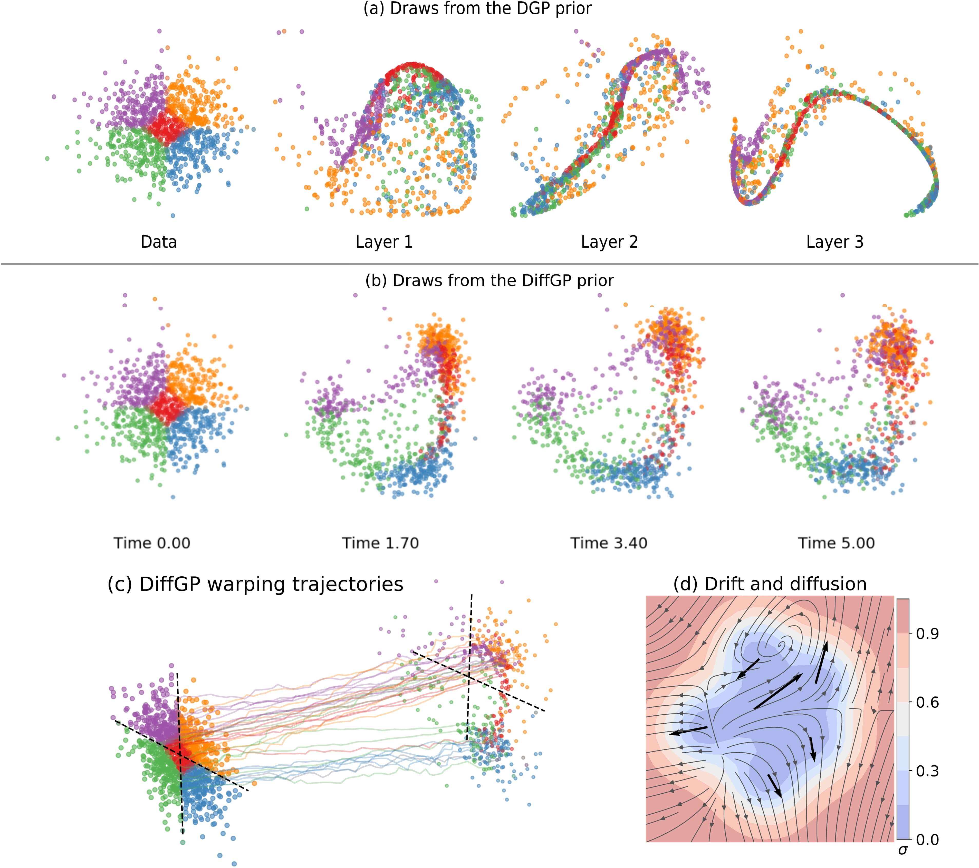
A deep Gaussian process $\mathbf{f}^{L}(\cdots\mathbf{f}^{2}(\mathbf{f}^{1}(\mathbf{x})))$ is a composition of $L$ Gaussian process layers $\mathbf{f}^{l}(\mathbf{x})$ (Damianou and Lawrence, 2013). These models typically lead to degenerate covariances, where each layer in the composition reduces the rank or degrees of freedom of the system (Duvenaud et al., 2014). In practice the rank reduces via successive layers mapping inputs to identical values (See Figure 3a), effectively merging inputs and resulting in a reduced-rank covariance matrix with repeated rows and columns. To counter this pathology Salimbeni and Deisenroth (2017) proposed pseudo-monotonic deep GPs by using identity mean function in all intermediate GP layers.

Unlike the earlier approaches, our model does not seem to suffer from this degeneracy. The DiffGP model warps the input space without seeking low-volume representations. In particular the SDE diffusion scatters the trajectories preventing both narrow manifolds and input merging. In practice, this results in a rank-preserving model (See Figure 3b-d). Therefore, we can use zero mean function for the Gaussian processes responsible for differential warpings.

4 EXPERIMENTS

		boston	energy	concrete	wine_red	kin8mn	power	naval	protein
	$N$	506	768	1,030	1,599	8,192	9,568	11,934	45,730
	$D$	13	8	8	22	8	4	26	9
Linear		4.24(0.16)	2.88(0.05)	10.54(0.13)	0.65(0.01)	0.20(0.00)	4.51(0.03)	0.01(0.00)	5.21(0.02)
BNN	$L=2$	3.01(0.18)	1.80(0.05)	5.67(0.09)	0.64(0.01)	0.10(0.00)	4.12(0.03)	0.01(0.00)	4.73(0.01)
Sparse GP	$M=100$	2.87(0.15)	0.78(0.02)	5.97(0.11)	0.63(0.01)	0.09(0.00)	3.91(0.03)	0.00(0.00)	4.43(0.03)
	$M=500$	2.73(0.12)	0.47(0.02)	5.53(0.12)	0.62(0.01)	0.08(0.00)	3.79(0.03)	0.00(0.00)	4.10(0.03)
Deep GP $M=100$	$L=2$	2.90(0.17)	0.47(0.01)	5.61(0.10)	0.63(0.01)	0.06(0.00)	3.79(0.03)	0.00(0.00)	4.00(0.03)
	$L=3$	2.93(0.16)	0.48(0.01)	5.64(0.10)	0.63(0.01)	0.06(0.00)	3.73(0.04)	0.00(0.00)	3.81(0.04)
	$L=4$	2.90(0.15)	0.48(0.01)	5.68(0.10)	0.63(0.01)	0.06(0.00)	3.71(0.04)	0.00(0.00)	3.74(0.04)
	$L=5$	2.92(0.17)	0.47(0.01)	5.65(0.10)	0.63(0.01)	0.06(0.00)	3.68(0.03)	0.00(0.00)	3.72(0.04)
DiffGP $M=100$	$T=1.0$	2.80(0.13)	0.49(0.02)	5.32(0.10)	0.63(0.01)	0.06(0.00)	3.76(0.03)	0.00(0.00)	4.04(0.04)
	$T=2.0$	2.68(0.10)	0.48(0.02)	4.96(0.09)	0.63(0.01)	0.06(0.00)	3.72(0.03)	0.00(0.00)	4.00(0.04)
	$T=3.0$	2.69(0.14)	0.47(0.02)	4.76(0.12)	0.63(0.01)	0.06(0.00)	3.68(0.03)	0.00(0.00)	3.92(0.04)
	$T=4.0$	2.67(0.13)	0.49(0.02)	4.65(0.12)	0.63(0.01)	0.06(0.00)	3.66(0.03)	0.00(0.00)	3.89(0.04)
	$T=5.0$	2.58(0.12)	0.50(0.02)	4.56(0.12)	0.63(0.01)	0.06(0.00)	3.65(0.03)	0.00(0.00)	3.87(0.04)

Table 1: Test RMSE values of 8 benchmark datasets (reproduced from Salimbeni & Deisenroth 2017). Uses random 90% / 10% training and test splits, repeated 20 times.

We optimize the inducing vectors, inducing locations, kernel lengthscales and signal variance of both the SDE function $\mathbf{f}$ equation (13) and the predictor function $g(\mathbf{x}_{T})$. We also optimize noise variance in problems with Gaussian likelihoods. The number of inducing points $M$ is manually chosen, where more inducing points tightens the variational approximation at the cost of additional computation. All parameters are jointly optimised against the evidence lower bound (38). The gradients of the lower bound back-propagate through the prediction function $g(\mathbf{x}_{T})$ and through the SDE system from $\mathbf{x}(T)$ back to initial values $\mathbf{x}(0)$. Gradients of an SDE system approximated by an EM method can be obtained with the autodiff differentiation of TensorFlow (Abadi et al., 2016). The gradients of continuous-time systems follow from forward or reverse mode sensitivity equations (Kokotovic and Heller, 1967; Raue et al., 2013; Fröhlich et al., 2017; Yildiz et al., 2018). We perform stochastic optimization with mini-batches and the Adam optimizer (Kingma and Ba, 2014) with a step size of 0.01. For numerical solutions of SDE, we use Euler-Maruyama solver with 20 time steps. Also, initializing parameters of $g(\cdot)$ with values learned through SGP results in early convergence; we initialize DiffGP training with SGP results and a very weak warping field ${\mathbf{U}_{\mathbf{f}}}\approx 0$ and kernel variance $\sigma_{f}^{2}\approx 0.01$. We use diagonal approximation of the ${\boldsymbol{\Sigma}}_{q}$. We also use GPflow (Matthews et al., 2017), a Gaussian processes framework built on TensorFlow in our implementation.

4.1 Step function estimation

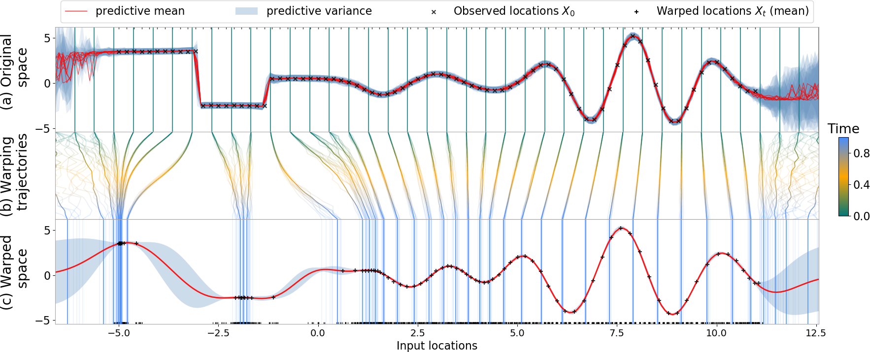
We begin by highlighting how the DiffGP estimates a signal with multiple highly non-stationary step functions. Figure 4 shows the univariate signal observations (top), the learned SDE flow (middle), and the resulting regression function on the end points $\mathbf{X}(t)$ (bottom). The DiffGP separates the regions around the step function such that the final regression function $g$ with a standard stationary Gaussian kernel can fit the transformed data $\mathbf{X}(t)$. The model then has learned the non-stationarities of the system with uncertainty in the signals being modelled by the inherent uncertainties arising from the diffusion.

Figure 4: Step function estimation: Observed input space (a) is transformed through stochastic continuous-time mappings (b) into a warped space (c). The stationary Gaussian process in the warped space gives a smooth predictive distribution corresponding to a highly non-stationary predictions in the original observed space.

4.2 UCI regression benchmarks

We compare our model on 8 regression benchmarks with the previously reported state-of-the-art results in (Salimbeni and Deisenroth, 2017). We test all the datasets on different flow time values from 1 to 5. We use the RBF kernel with ARD and 100 inducing points for both the differential Gaussian Process and the regression Gaussian Process. Each experiment is repeated 20 times with random 90% / 10% training and test splits. While testing, we compute predictive mean and predictive variance for each of the sample generated from (37), and compute the average of summary statistics (RMSE and log likelihood) over these samples. The mean and standard error of RMSE values are reported in Table 1.

On Boston, Concrete and Power datasets, where deep models show improvement over shallow models, our model outperforms previous best results of DGP. There is a small improvement by having a non-linear model on the Kin8mn dataset and our results match that of DGP. Energy and Wine are small datasets where single Gaussian Processes perform the best. As expected, both DiffGP and DGP recover the shallow model indicating no over-fitting. Regression task on the Protein dataset is aimed at predicting RMSD (Root Mean Squared Deviation) between modeled and native protein structures using 9 different properties of the modeled structures (Rana et al., 2015). We suspect DGP particularly performs better than DiffGP in the task because of its capability to model long-range correlations.

4.3 UCI classification benchmarks

We perform binary classification experiments on large-scale HIGGS and SUSY datasets with a data size in the order of millions. We use the AUC as the performance measure and compare the results with the previously reported results using DGP (Salimbeni and Deisenroth, 2017) and DNN (Baldi et al., 2014). The classification task involves identifying processes that produce Higgs boson and super-symmetric particles using data from Monte Carlo simulations. Previously, deep learning methods based on neural networks have shown promising results on these tasks (Baldi et al., 2014). On the HIGGS dataset, the proposed DiffGP model shows state-of-the-art (0.878) results, equal or even better than the earlier reported results using DGPs (0.877) and DNNs (0.876). On the SUSY dataset, we reach the performance of 4-hidden layer DGP (0.841) with non-temporal DiffGP (0.842). Considering the consistent improvement in the performance of DGP models with additional layers, we tried increasing the capacity of DiffGP model using the temporal extension proposed in Section 3.1. In particular, we used 100 spatial inducing vectors along with 3 temporal inducing vectors. The temporal DiffGP model gives an AUC of 0.878 on HIGGS and 0.846 on SUSY datasets matching the best reported results of DGP (see appendix for detailed comparison).

4.4 Importance of flow time

Figure 5: Concrete dataset: increasing the flow time variable $T$ improves the train and test errors (a,c) and likelihoods (b,d). The horizontal line indicates GP and DGP2 performance. The model convergence indicates the improved capacity upon increased flow time (e).

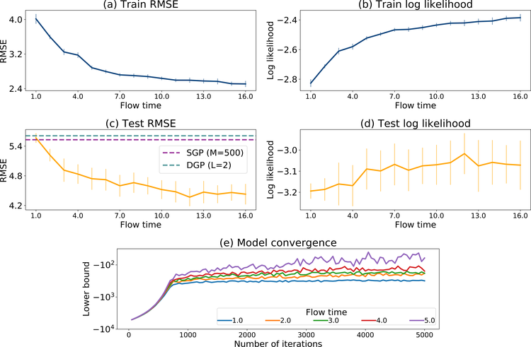
In this we experiment we study the SDE flow time parameter on Concrete dataset. Increasing integration time provides more warping flexibility to the SDE warping component. That is, with increase in the flow time, the SDE system can move observations further away from the initial state, however at the cost of exposing the state to more diffusion which acts as a principled regularization. Thus increasing time can lead to an increase in the model capacity without over-fitting. We empirically support this claim in the current experiment by fitting a regression model multiple times and maintaining same experimental setup, expect for the flow time. Figure 5 shows the variation in RMSE, log likelihood and the lower bound on marginal likelihood across different flow times. It can be seen that the improvement in the performance almost saturates near time = $10$.

5 DISCUSSION

We have proposed a novel paradigm, continuous-time Gaussian process deep learning. The proposed deferentially deep composition is a continuous-time approach wherein a Gaussian processes input locations are warped through stochastic and smooth differential equations. This results in a principled Bayesian approach with a smooth non-linear warping; the uncertainty through diffusion acts as a key regularizer.

We empirically show excellent results in various regression and classification tasks. Also, DGP with the model specification as proposed by Salimbeni and Deisenroth (2017), uses a total of $\mathcal{O}(LDM)$ number of inducing parameters for the regression results, where $L$ is the number of layers, $D$ is the input dimension, $M$ is the number of inducing points for each latent GP. In contrast, with a smaller number of inducing parameters $\mathcal{O}(DM)$, we arrive at similar or even better results.

The continuous-time deep model admits ‘decision-making paths’, where we can explicitly follow the transformation applied to a data point $\mathbf{x}_{i}$. Analyzing these paths could lead to a better interpretable model. However, modeling in the input space without intermediate low-dimensional latent representations presents scalability issues. We leave scaling the approach to high dimensions as future work, while we also intend to explore new optimisation modes, such as SG-MCMC (Ma et al., 2015) or Stein inference (Liu and Wang, 2016) in the future.

APPENDIX

A. Derivation of the stochastic variational inference

The differential Gaussian process is a combination of a conventional prediction GP $g(\cdot)$ with an SDE flow GP $\mathbf{f}(\cdot)$ fully parameterised by $\mathbf{Z},\mathbf{U}$ as well as kernel parameters $\theta$. We turn to variational inference to estimate posterior approximations $q({\mathbf{U}_{\mathbf{f}}})$ and $q(\mathbf{u}_{g})$ for both models.

Exact inference of Gaussian processes has a limiting complexity of $\mathcal{O}(N^{3})$. Instead, we apply stochastic variational inference (SVI) (Hensman et al., 2015), which has been demonstrated to scale GP’s up to a billion data points (Salimbeni and Deisenroth, 2017). We here summarise the SVI procedure following Hensman et al. (2015).

We start with the joint density of a single path and prediction of the augmented system

$$p(\mathbf{y},{\mathbf{g}},{\mathbf{u}_{g}},{\mathbf{X}_{T}},\mathbf{f},{\mathbf{U}_{\mathbf{f}}})=\underbrace{p(\mathbf{y}|{\mathbf{g}})}_{\text{likelihood}}\underbrace{p({\mathbf{g}}|{\mathbf{u}_{g}},{\mathbf{X}_{T}})p({\mathbf{u}_{g}})}_{\text{GP prior of $g(\mathbf{x})$}}\underbrace{p({\mathbf{X}_{T}}|\mathbf{f})}_{\text{SDE}}\underbrace{p(\mathbf{f}|{\mathbf{U}_{\mathbf{f}}})p({\mathbf{U}_{\mathbf{f}}})}_{\text{GP prior of $\mathbf{f}(\mathbf{x})$}}.$$ (39)

where we have augmented the predictor function $g$ with $M$ inducing locations ${\mathbf{Z}_{g}}=(\mathbf{z}_{g1},\ldots,\mathbf{z}_{gM})$ with associated inducing function values $g(\mathbf{z})=u$ in a vector ${\mathbf{u}_{g}}=(u_{g1},\ldots,u_{gM})^{T}\in\mathbb{R}^{M}$ with a GP prior. The conditional distribution is (Titsias, 2009)

$$p({\mathbf{g}}|{\mathbf{u}_{g}},{\mathbf{X}_{T}}) =\mathcal{N}({\mathbf{g}}|\mathbf{Q}_{T}{\mathbf{u}_{g}},\mathbf{K}_{{\mathbf{X}_{T}}{\mathbf{X}_{T}}}-\mathbf{Q}_{T}\mathbf{K}_{{\mathbf{Z}_{g}}{\mathbf{Z}_{g}}}\mathbf{Q}_{T}^{T})$$ (40)

$$p({\mathbf{u}_{g}}) =\mathcal{N}({\mathbf{u}_{g}}|\mathbf{0},\mathbf{K}_{{\mathbf{Z}_{g}}{\mathbf{Z}_{g}}}),$$ (41)

where we denote $\mathbf{Q}_{T}=\mathbf{K}_{{\mathbf{X}_{T}}{\mathbf{Z}_{g}}}\mathbf{K}_{{\mathbf{Z}_{g}}{\mathbf{Z}_{g}}}^{-1}$.

Similarly, the warping function $\mathbf{f}$ is augmented with inducing variables $\mathbf{u}_{\mathbf{f}d}=(\mathbf{u}_{1}^{f}(d)^{T},\ldots,\mathbf{u}_{M}^{f}(d))$ and inducing locations ${\mathbf{Z}_{\mathbf{f}}}_{d}=(\mathbf{z}_{1}^{f}(d),\ldots,\mathbf{z}_{M}^{f}(d))^{T}$.

$$p({\mathbf{U}_{\mathbf{f}}}) =\prod_{d=1}^{D}\mathcal{N}(\mathbf{u}_{\mathbf{f}d}|\mathbf{0},\mathbf{K}_{{\mathbf{Z}_{\mathbf{f}}}_{d}{\mathbf{Z}_{\mathbf{f}}}_{d}}),$$ (42)

The joint distribution (39) contains the likelihood term, the two GP priors, and the SDE term $p({\mathbf{X}_{T}}|\mathbf{f})$ representing the Euler-Maruyama paths of the dataset.

$$d\mathbf{x}_{t} ={\boldsymbol{\mu}}(\mathbf{x}_{t})dt+\sqrt{\Sigma(\mathbf{x}_{t})}dW_{t}$$ (43)

$${\boldsymbol{\mu}}(\mathbf{x}_{t}) =\mathbf{R}{\mathbf{U}_{\mathbf{f}}}$$ (44)

$${\boldsymbol{\Sigma}}(\mathbf{x}_{t}) =\mathbf{K}_{\mathbf{x}\mathbf{x}}-\mathbf{R}\mathbf{K}_{{\mathbf{Z}_{\mathbf{f}}}{\mathbf{Z}_{\mathbf{f}}}}\mathbf{R}$$ (45)

We consider optimizing the marginal likelihood

$$\log p(\mathbf{y}) =\log\mathbb{E}_{p({\mathbf{g}}|{\mathbf{X}_{T}})p({\mathbf{X}_{T}})}p(\mathbf{y}|{\mathbf{g}}),$$ (46)

$$p({\mathbf{g}}|{\mathbf{X}_{T}}) =\int p({\mathbf{g}}|{\mathbf{u}_{g}},{\mathbf{X}_{T}})p({\mathbf{u}_{g}})d{\mathbf{u}_{g}}$$ (47)

$$p({\mathbf{X}_{T}}) =\iint p({\mathbf{X}_{T}}|\mathbf{f})p(\mathbf{f}|{\mathbf{U}_{\mathbf{f}}})p({\mathbf{U}_{\mathbf{f}}})d\mathbf{f}d{\mathbf{U}_{\mathbf{f}}},$$ (48)

with no tractable solution due to the FPK state distribution $p({\mathbf{X}_{T}})$.

A variational lower bound for the evidence (46) without the state distributions has already been considered by Hensman et al. (2015). We propose to include the state distributions by simulating Monte Carlo state trajectories.

We propose a complete variational posterior approximation over both $\mathbf{f}$ and $g$,

$$q({\mathbf{g}},{\mathbf{u}_{g}},{\mathbf{X}_{T}},\mathbf{f},{\mathbf{U}_{\mathbf{f}}}) =p({\mathbf{g}}|{\mathbf{u}_{g}},{\mathbf{X}_{T}})q({\mathbf{u}_{g}})p({\mathbf{X}_{T}}|\mathbf{f})p(\mathbf{f}|{\mathbf{U}_{\mathbf{f}}})q({\mathbf{U}_{\mathbf{f}}})$$ (49)

$$q({\mathbf{u}_{g}}) =\mathcal{N}({\mathbf{u}_{g}}|{\mathbf{m}_{g}},{\mathbf{S}_{g}})$$ (50)

$$q({\mathbf{U}_{\mathbf{f}}}) =\prod_{d=1}^{D}\mathcal{N}(\mathbf{u}_{\mathbf{f}d}|\mathbf{m}_{\mathbf{f}d},\mathbf{S}_{\mathbf{f}d}),$$ (51)

where $\mathbf{M}_{\mathbf{f}}=(\mathbf{m}_{\mathbf{f}1},\ldots,\mathbf{m}_{\mathbf{f}D})$ and ${\mathbf{S}_{\mathbf{f}}}=(\mathbf{S}_{\mathbf{f}1},\ldots,\mathbf{S}_{\mathbf{f}D})$ collect the dimension-wise inducing parameters. We continue by marginalizing out inducing variables ${\mathbf{u}_{g}}$ and ${\mathbf{U}_{\mathbf{f}}}$ from the above joint distribution arriving at the joint variational posterior

$$q({\mathbf{g}},{\mathbf{X}_{T}},\mathbf{f}) =q({\mathbf{g}}|{\mathbf{X}_{T}})p({\mathbf{X}_{T}}|\mathbf{f})q(\mathbf{f}),$$ (52)

where

$$q({\mathbf{g}}|{\mathbf{X}_{T}}) =\int p({\mathbf{g}}|{\mathbf{u}_{g}},{\mathbf{X}_{T}})q({\mathbf{u}_{g}})d{\mathbf{u}_{g}}$$ (53)

$$=\mathcal{N}({\mathbf{g}}|\mathbf{Q}_{T}{\mathbf{m}_{g}},\mathbf{K}_{{\mathbf{X}_{T}}{\mathbf{X}_{T}}}+\mathbf{Q}_{T}({\mathbf{S}_{g}}-\mathbf{K}_{{\mathbf{Z}_{g}}{\mathbf{Z}_{g}}})\mathbf{Q}_{T}^{T})$$ (54)

$$q(\mathbf{f}) =\int p(\mathbf{f}|{\mathbf{U}_{\mathbf{f}}})q({\mathbf{U}_{\mathbf{f}}})d{\mathbf{U}_{\mathbf{f}}}$$ (55)

$$=\mathcal{N}(\mathbf{f}|{\boldsymbol{\mu}}_{q},{\boldsymbol{\Sigma}}_{q})$$

$${\boldsymbol{\mu}}_{q} =\mathbf{Q}_{\mathbf{f}}\mathbf{M}_{\mathbf{f}}$$ (56)

$${\boldsymbol{\Sigma}}_{q} =\mathbf{K}_{\mathbf{X}\mathbf{X}}+\mathbf{Q}_{\mathbf{f}}({\mathbf{S}_{\mathbf{f}}}-\mathbf{K}_{{\mathbf{Z}_{\mathbf{f}}}{\mathbf{Z}_{\mathbf{f}}}})\mathbf{Q}_{\mathbf{f}}^{T}$$ (57)

where $\mathbf{Q}_{\mathbf{f}}=\mathbf{K}_{\mathbf{X}{\mathbf{Z}_{\mathbf{f}}}}\mathbf{K}_{{\mathbf{Z}_{\mathbf{f}}}{\mathbf{Z}_{\mathbf{f}}}}^{-1}$. We plug the derived variational posterior drift ${\boldsymbol{\mu}}_{q}$ and diffusion ${\boldsymbol{\Sigma}}_{q}$ estimates to the SDE to arrive at the final variational SDE flow

$$d\mathbf{x}_{t} ={\boldsymbol{\mu}}_{q}(\mathbf{x}_{t})dt+\sqrt{{\boldsymbol{\Sigma}}_{q}(\mathbf{x}_{t})}dW_{t},$$ (58)

which conveniently encodes the variational approximation of $\mathbf{f}$.

Now the lower bound for our differential deep GP model can be written as

$$\log p(\mathbf{y}) \geq\int q({\mathbf{g}},{\mathbf{u}_{g}},{\mathbf{X}_{T}},\mathbf{f},{\mathbf{U}_{\mathbf{f}}})\log\frac{p(\mathbf{y},{\mathbf{g}},{\mathbf{u}_{g}},{\mathbf{X}_{T}},\mathbf{f},{\mathbf{U}_{\mathbf{f}}})}{q({\mathbf{g}},{\mathbf{u}_{g}},{\mathbf{X}_{T}},\mathbf{f},{\mathbf{U}_{\mathbf{f}}})}d{\mathbf{g}}d{\mathbf{u}_{g}}d{\mathbf{X}_{T}}d\mathbf{f}d{\mathbf{U}_{\mathbf{f}}}$$ (59)

$$\geq\int p({\mathbf{g}}|{\mathbf{u}_{g}},{\mathbf{X}_{T}})q({\mathbf{u}_{g}})p({\mathbf{X}_{T}}|\mathbf{f})p(\mathbf{f}|{\mathbf{U}_{\mathbf{f}}})q({\mathbf{U}_{\mathbf{f}}})\log\frac{p(\mathbf{y}|{\mathbf{g}})p({\mathbf{u}_{g}})p({\mathbf{U}_{\mathbf{f}}})}{q({\mathbf{u}_{g}})q({\mathbf{U}_{\mathbf{f}}})}d{\mathbf{g}}d{\mathbf{u}_{g}}d{\mathbf{X}_{T}}d\mathbf{f}d{\mathbf{U}_{\mathbf{f}}}$$ (60)

$$\geq\int q({\mathbf{g}}|{\mathbf{X}_{T}})q({\mathbf{X}_{T}})\log p(\mathbf{y}|{\mathbf{g}})d{\mathbf{g}}d{\mathbf{X}_{T}}-\operatorname{\textsc{kl}}[q({\mathbf{u}_{g}})||p({\mathbf{u}_{g}})]-\operatorname{\textsc{kl}}[q({\mathbf{U}_{\mathbf{f}}})||p({\mathbf{U}_{\mathbf{f}}})]$$ (61)

$$\geq\sum_{i=1}^{N}\bigg{\{}\frac{1}{S}\sum_{s=1}^{S}\underbrace{\mathbb{E}_{q({\mathbf{g}}|\mathbf{x}_{i,T}^{(s)})}\log p(y_{i}|g_{i})}_{\text{variational expected likelihood}}-\underbrace{\operatorname{\textsc{kl}}[q({\mathbf{u}_{g}})||p({\mathbf{u}_{g}})]}_{\text{$g(x)$ prior divergence}}-\underbrace{\operatorname{\textsc{kl}}[q({\mathbf{U}_{\mathbf{f}}})||p({\mathbf{U}_{\mathbf{f}}})]}_{\text{$\mathbf{f}(x)$ prior divergence}}\bigg{\}}.$$ (62)

B. Regression and classification benchmarks

		boston	energy	concrete	wine_red	kin8mn	power	naval	protein
	$N$	506	768	1,030	1,599	8,192	9,568	11,934	45,730
	$D$	13	8	8	22	8	4	26	9
Linear		4.24(0.16)	2.88(0.05)	10.54(0.13)	0.65(0.01)	0.20(0.00)	4.51(0.03)	0.01(0.00)	5.21(0.02)
BNN	$L=2$	3.01(0.18)	1.80(0.05)	5.67(0.09)	0.64(0.01)	0.10(0.00)	4.12(0.03)	0.01(0.00)	4.73(0.01)
Sparse GP	$M=100$	2.87(0.15)	0.78(0.02)	5.97(0.11)	0.63(0.01)	0.09(0.00)	3.91(0.03)	0.00(0.00)	4.43(0.03)
	$M=500$	2.73(0.12)	0.47(0.02)	5.53(0.12)	0.62(0.01)	0.08(0.00)	3.79(0.03)	0.00(0.00)	4.10(0.03)
Deep GP $M=100$	$L=2$	2.90(0.17)	0.47(0.01)	5.61(0.10)	0.63(0.01)	0.06(0.00)	3.79(0.03)	0.00(0.00)	4.00(0.03)
	$L=3$	2.93(0.16)	0.48(0.01)	5.64(0.10)	0.63(0.01)	0.06(0.00)	3.73(0.04)	0.00(0.00)	3.81(0.04)
	$L=4$	2.90(0.15)	0.48(0.01)	5.68(0.10)	0.63(0.01)	0.06(0.00)	3.71(0.04)	0.00(0.00)	3.74(0.04)
	$L=5$	2.92(0.17)	0.47(0.01)	5.65(0.10)	0.63(0.01)	0.06(0.00)	3.68(0.03)	0.00(0.00)	3.72(0.04)
DiffGP $M=100$	$T=1.0$	2.80(0.13)	0.49(0.02)	5.32(0.10)	0.63(0.01)	0.06(0.00)	3.76(0.03)	0.00(0.00)	4.04(0.04)
	$T=2.0$	2.68(0.10)	0.48(0.02)	4.96(0.09)	0.63(0.01)	0.06(0.00)	3.72(0.03)	0.00(0.00)	4.00(0.04)
	$T=3.0$	2.69(0.14)	0.47(0.02)	4.76(0.12)	0.63(0.01)	0.06(0.00)	3.68(0.03)	0.00(0.00)	3.92(0.04)
	$T=4.0$	2.67(0.13)	0.49(0.02)	4.65(0.12)	0.63(0.01)	0.06(0.00)	3.66(0.03)	0.00(0.00)	3.89(0.04)
	$T=5.0$	2.58(0.12)	0.50(0.02)	4.56(0.12)	0.63(0.01)	0.06(0.00)	3.65(0.03)	0.00(0.00)	3.87(0.04)

Table 2: Test RMSE values of 8 benchmark datasets (reproduced from from Salimbeni & Deisenroth 2017). Uses random 90% / 10% training and test splits, repeated 20 times.

		boston	energy	concrete	wine_red	kin8mn	power	naval	protein
	$N$	506	768	1,030	1,599	8,192	9,568	11,934	45,730
	$D$	13	8	8	22	8	4	26	9
Linear		-2.89(0.03)	-2.48(0.02)	-3.78(0.01)	-0.99(0.01)	0.18(0.01)	-2.93(0.01)	3.73(0.00)	-3.07(0.00)
BNN	$L=2$	-2.57(0.09)	-2.04(0.02)	-3.16(0.02)	-0.97(0.01)	0.90(0.01)	-2.84(0.01)	3.73(0.01)	-2.97(0.00)
Sparse GP	$M=100$	-2.47(0.05)	-1.29(0.02)	-3.18(0.02)	-0.95(0.01)	0.63(0.01)	-2.75(0.01)	6.57(0.15)	-2.91(0.00)
	$M=500$	-2.40(0.07)	-0.63(0.03)	-3.09(0.02)	-0.93(0.01)	1.15(0.00)	-2.75(0.01)	7.01(0.05)	-2.83(0.00)
Deep GP $M=100$	$L=2$	-2.47(0.05)	-0.73(0.02)	-3.12(0.01)	-0.95(0.01)	1.34(0.01)	-2.75(0.01)	6.76(0.19)	-2.81(0.00)
	$L=3$	-2.49(0.05)	-0.75(0.02)	-3.13(0.01)	-0.95(0.01)	1.37(0.01)	-2.74(0.01)	6.62(0.18)	-2.75(0.00)
	$L=4$	-2.48(0.05)	-0.76(0.02)	-3.14(9 .01)	-0.95(0.01)	1.38(0.01)	-2.74(0.01)	6.61(0.17)	-2.73(0.00)
	$L=5$	-2.49(0.05)	-0.74(0.02)	-3.13(0.01)	-0.95(0.01)	1.38(0.01)	-2.73(0.01)	6.41(0.28)	-2.71(0.00)
DiffGP $M=100$	$T=1.0$	-2.36(0.05)	-0.65(0.03)	-3.05(0.02)	-0.96(0.01)	1.36(0.01)	-2.75(0.01)	6.58(0.02)	-2.79(0.04)
	$T=2.0$	-2.32(0.04)	-0.63(0.03)	-2.96(0.02)	-0.97(0.02)	1.37(0.00)	-2.74(0.01)	6.26(0.03)	-2.78(0.04)
	$T=3.0$	-2.31(0.05)	-0.63(0.02)	-2.93(0.04)	-0.97(0.02)	1.37(0.01)	-2.72(0.01)	6.00(0.03)	-2.79(0.00)
	$T=4.0$	-2.33(0.06)	-0.65(0.02)	-2.91(0.04)	-0.98(0.02)	1.37(0.01)	-2.72(0.01)	5.86(0.02)	-2.78(0.00)
	$T=5.0$	-2.30(0.05)	-0.66(0.02)	-2.90(0.05)	-0.98(0.02)	1.36(0.01)	-2.72(0.01)	5.78(0.02)	-2.77(0.00)

Table 3: Test log likelihood values of 8 benchmark datasets (reproduced from from Salimbeni & Deisenroth 2017)

		SUSY	HIGGS
	$N$	5,500,000	11,000,000
	$D$	18	28
DNN		0.876	0.885
Sparse GP	$M=100$	0.875	0.785
	$M=500$	0.876	0.794
Deep GP $M=100$	$L=2$	0.877	0.830
	$L=3$	0.877	0.837
	$L=4$	0.877	0.841
	$L=5$	0.877	0.846
DiffGP $M=100$	$t=1.0$	0.878	0.840
	$t=3.0$	0.878	0.841
	$t=5.0$	0.878	0.842
DiffGP Temporal $M_{s}=100$ $M_{t}=3$
	$t=5.0$	0.878	0.846

Table 4: Test AUC values for large-scale classification datasets. Uses random 90% / 10% training and test splits.

References

- Abadi et al. (2016) Martín Abadi, Paul Barham, Jianmin Chen, Zhifeng Chen, Andy Davis, Jeffrey Dean, Matthieu Devin, Sanjay Ghemawat, Geoffrey Irving, Michael Isard, et al. Tensorflow: A system for large-scale machine learning. In OSDI, volume 16, pages 265–283, 2016.
- Baldi et al. (2014) Pierre Baldi, Peter Sadowski, and Daniel Whiteson. Searching for exotic particles in high-energy physics with deep learning. Nature Communications, 5:4308, 2014.
- Blei et al. (2016) D. Blei, A. Kucukelbir, and J. McAuliffe. Variational inference: A review for statisticians. Journal of the American Statistical Association, 112:859–877, 2016.
- Damianou and Lawrence (2013) Andreas Damianou and Neil Lawrence. Deep gaussian processes. In Artificial Intelligence and Statistics, pages 207–215, 2013.
- Duvenaud et al. (2014) David Duvenaud, Oren Rippel, Ryan Adams, and Zoubin Ghahramani. Avoiding pathologies in very deep networks. In Artificial Intelligence and Statistics, pages 202–210, 2014.
- Duvenaud et al. (2011) David K Duvenaud, Hannes Nickisch, and Carl E Rasmussen. Additive gaussian processes. In Advances in Neural Information Processing Systems, pages 226–234, 2011.
- Friedrich et al. (2011) Rudolf Friedrich, Joachim Peinke, Muhammad Sahimi, and M Reza Rahimi Tabar. Approaching complexity by stochastic methods: From biological systems to turbulence. Physics Reports, 506(5):87–162, 2011.
- Fröhlich et al. (2017) Fabian Fröhlich, Barbara Kaltenbacher, Fabian J. Theis, and Jan Hasenauer. Scalable parameter estimation for genome-scale biochemical reaction networks. PLOS Computational Biology, 13(1):1–18, 01 2017. doi: 10.1371/journal.pcbi.1005331.
- García et al. (2017) C. García, A. Otero, P. Felix, J. Presedo, and D. Marquez. Nonparametric estimation of stochastic differential equations with sparse Gaussian processes. Physical Review E, 96(2):022104, 2017.
- Heinonen et al. (2016) M. Heinonen, H. Mannerström, J. Rousu, S. Kaski, and H. Lähdesmäki. Non-stationary Gaussian process regression with Hamiltonian Monte Carlo. In AISTATS, volume 51, pages 732–740, 2016.
- Hensman et al. (2013) J. Hensman, N. Fusi, and N. Lawrence. Gaussian processes for big data. In Proceedings of the Twenty-Ninth Conference on Uncertainty in Artificial Intelligence, pages 282–290. AUAI Press, 2013.
- Hensman et al. (2015) J. Hensman, A. Matthews, and Z. Ghahramani. Scalable variational Gaussian process classification. In Artificial Intelligence and Statistics, pages 351–360, 2015.
- Higham (2001) Desmond Higham. An algorithmic introduction to numerical simulation of stochastic differential equations. SIAM Rev., 43:525–546, 2001.
- Kingma and Ba (2014) Diederik P Kingma and Jimmy Lei Ba. Adam: Amethod for stochastic optimization. In Proc. 3rd Int. Conf. Learn. Representations, 2014.
- Kloeden and Platen (1992) P.E. Kloeden and E. Platen. Numerical Solution of Stochastic Differential Equations. Applications of Mathematics. Springer-Verlag, 1992. ISBN 9783540540625. URL https://books.google.fi/books?id=7bkZAQAAIAAJ.
- Kokotovic and Heller (1967) P Kokotovic and J Heller. Direct and adjoint sensitivity equations for parameter optimization. IEEE Transactions on Automatic Control, 12(5):609–610, 1967.
- Lamba et al. (2006) H Lamba, Jonathan C Mattingly, and Andrew M Stuart. An adaptive euler–maruyama scheme for sdes: convergence and stability. IMA journal of numerical analysis, 27:479–506, 2006.
- Lázaro-Gredilla (2012) Miguel Lázaro-Gredilla. Bayesian warped gaussian processes. In Advances in Neural Information Processing Systems, pages 1619–1627, 2012.
- Liu and Wang (2016) Qiang Liu and Dilin Wang. Stein variational gradient descent: A general purpose bayesian inference algorithm. In Advances in Neural Information Processing Systems, pages 2378–2386, 2016.
- Ma et al. (2015) Yi-An Ma, Tianqi Chen, and Emily Fox. A complete recipe for stochastic gradient mcmc. In Advances in Neural Information Processing Systems, pages 2917–2925, 2015.
- Matthews et al. (2017) Alexander G. de G. Matthews, Mark van der Wilk, Tom Nickson, Keisuke. Fujii, Alexis Boukouvalas, Pablo León-Villagrá, Zoubin Ghahramani, and James Hensman. GPflow: A Gaussian process library using TensorFlow. Journal of Machine Learning Research, 18(40):1–6, apr 2017. URL http://jmlr.org/papers/v18/16-537.html.
- Oksendal (2014) B. Oksendal. Stochastic Differential Equations: An Introduction with Applications. Springer, 6th edition, 2014.
- Papaspiliopoulos et al. (2012) Omiros Papaspiliopoulos, Yvo Pokern, Gareth O Roberts, and Andrew M Stuart. Nonparametric estimation of diffusions: a differential equations approach. Biometrika, 99(3):511–531, 2012.
- Rana et al. (2015) Prashant Singh Rana, Harish Sharma, Mahua Bhattacharya, and Anupam Shukla. Quality assessment of modeled protein structure using physicochemical properties. Journal of bioinformatics and computational biology, 13(02):1550005, 2015.
- Rasmussen and Williams (2006) C.E. Rasmussen and K.I. Williams. Gaussian processes for machine learning. MIT Press, 2006.
- Raue et al. (2013) Andreas Raue, Marcel Schilling, Julie Bachmann, Andrew Matteson, Max Schelker, Daniel Kaschek, Sabine Hug, Clemens Kreutz, Brian D. Harms, Fabian J. Theis, Ursula Klingmüller, and Jens Timmer. Lessons learned from quantitative dynamical modeling in systems biology. PLOS ONE, 8(9):1–17, 2013.
- Remes et al. (2017) S. Remes, M. Heinonen, and S. Kaski. Non-stationary spectral kernels. Advances in Neural Information Processing Systems, 2017.
- Salimbeni and Deisenroth (2017) Hugh Salimbeni and Marc Deisenroth. Doubly stochastic variational inference for deep gaussian processes. In Advances in Neural Information Processing Systems, pages 4591–4602, 2017.
- Snelson and Ghahramani (2006) Edward Snelson and Zoubin Ghahramani. Sparse gaussian processes using pseudo-inputs. In Advances in Neural Information Processing Systems, pages 1257–1264, 2006.
- Snelson et al. (2004) Edward Snelson, Zoubin Ghahramani, and Carl E Rasmussen. Warped gaussian processes. In Advances in Neural Information Processing Systems, pages 337–344, 2004.
- Snoek et al. (2014) Jasper Snoek, Kevin Swersky, Rich Zemel, and Ryan Adams. Input warping for bayesian optimization of non-stationary functions. In International Conference on Machine Learning, pages 1674–1682, 2014.
- Stegle et al. (2011) Oliver Stegle, Christoph Lippert, Joris M Mooij, Neil D Lawrence, and Karsten M Borgwardt. Efficient inference in matrix-variate gaussian models with iid observation noise. In Advances in neural information processing systems, pages 630–638, 2011.
- Sun et al. (2018) S. Sun, G. Zhang, C. Wang, W. Zeng, J. Li, and R. Grosse. Differentiable compositional kernel learning for gaussian processes. In International Conference on Machine Learning, 2018.
- Titsias (2009) M. Titsias. Variational learning of inducing variables in sparse Gaussian processes. In Artificial Intelligence and Statistics, pages 567–574, 2009.
- Tolvanen et al. (2014) Ville Tolvanen, Pasi Jylänki, and Aki Vehtari. Expectation propagation for nonstationary heteroscedastic gaussian process regression. In Machine Learning for Signal Processing (MLSP), 2014 IEEE International Workshop on, pages 1–6. IEEE, 2014.
- Wilson et al. (2013) A. Wilson, E. Gilboa, A. Nehorai, and J. Cunningham. Fast multidimensional pattern extrapolation with gaussian processes. Artificial Intelligence and Statistics, 2013.
- Wilson et al. (2012) Andrew Gordon Wilson, David A Knowles, and Zoubin Ghahramani. Gaussian process regression networks. In Proceedings of the 29th International Coference on International Conference on Machine Learning, pages 1139–1146. Omnipress, 2012.
- Wilson et al. (2016) Andrew Gordon Wilson, Zhiting Hu, Ruslan Salakhutdinov, and Eric P Xing. Deep kernel learning. In Artificial Intelligence and Statistics, pages 370–378, 2016.
- Yildiz et al. (2018) Cagatay Yildiz, Markus Heinonen, Jukka Intosalmi, Henrik Mannerström, and Harri Lähdesmäki. Learning stochastic differential equations with gaussian processes without gradient matching. In Machine Learning in Signal Processing, 2018.