The impact of speckle disorder on a superfluid Fermi system

Abstract

Optical lattice experiments which probe the effect of disorder on superfluidity often use a speckle pattern for generating the disorder. Such speckle disorder is spatially correlated. While fermionic superfluidity in the presence of uncorrelated disorder is well studied, the impact of correlated disorder, particularly on thermal properties of the superfluid, is poorly understood. We provide a detailed study of the impact of speckle disorder, for varying speckle size and disorder magnitude, on the ground state and thermal properties of a Fermi superfluid. We work in the coupling regime of BCS-BEC crossover in a two dimensional lattice. For a fixed disorder strength, an increase in speckle size leads to smoothening of the self-consistent background potential, increase in the critical disorder needed for a superfluid-insulator transition, and an increase in superfluid $T_{c}$. Along with these hints at decrease in effective disorder, speckle correlations also suppress the superfluid gap and the gap formation temperature - effects normally associated with increasing disorder. We correlate these effects with the effective potential and the single particle localisation effects in the ground state.

I Introduction

Fermi superfluids with $s$-wave symmetry are robust to the presence of weak disorder anderson ; ag . In two dimensions, where all states are localised in the presence of arbitrarily weak disorder andloc-2d , and the non interacting system would be an insulator, the presence of pairing interaction leads to a superfluid (SF) state sit-revs . The interplay of disorder and pairing on the survival of a superfluid ground state has been extensively explored both theoretically ghosal-prb ; triv-1996 ; dag ; dubi ; bouadim and experimentally haviland-prl ; shahar-ovad ; escoffier-2004 ; baturina-2007 . Most of the earlier experiments are on the solid state, where multiple interactions may be at play, but artificially engineered optical lattices jaks ; ess ; bloch now provide a controlled option.

Weak coupling superfluidity in the presence of disorder was first examined by Anderson anderson , leading to what is called ‘Anderson’s theorem’ about the insensitivity of the SF state to weak disorder. This insight has been put on firmer ground by solution ghosal-prb of the Bogoliubov-de Gennes (BdG) equations for disordered SF’s, explicitly solving for the spatially modulated pairing amplitude. This leads to significant predictions about cluster formation and survival of the spectral gap across the disorder driven SF to insulator transition (SIT). Thermal effects can be reasonably accessed within the BdG scheme at weak coupling. Complications arise when one moves beyond the weak coupling ‘BCS’ window Meir1 ; Meir2 ; tarat1 ; tarat2 ; th-int-fermi4 .

For interactions beyond the BCS regime phase fluctuations of the order parameter, which are neglected in a BdG scheme, become significant. Disorder makes the phase stiffness spatially inhomogeneous, and worsens this situation. Phase fluctuation between weakly coupled clusters can destroy global coherence with SF order surviving in patches. This calls for an approach that treats thermal fluctuation of the order parameter in an inhomogeneous situation. Full quantum Monte Carlo triv-1996 ; bouadim accomplishes this, and we have shown earlier that a simpler method tarat1 ; tarat2 can also capture the thermal physics. The uncorrelated disorder problem is reasonably understood even beyond weak coupling.

It is interesting to ask how spatial correlations in the disorder - as in disordered optical lattices - modify the physics. The ‘speckle disorder’ in these systems is characterised by two parameters: the scale $V$ of potential fluctuations, and the correlation length, $\sigma$. Some of the effects of spatial correlations in the disorder have been probed by theory. For non interacting systems, transport in a speckle disorder potential requires revision of many results that exist in the case of uncorrelated disorder. Several studies have been done on this th-non-int1 ; th-non-int2 ; th-non-int3 ; th-non-int4 ; th-non-int5 ; th-non-int6 ; th-non-int7 ; th-non-int8 ; th-non-int9 modifying the Boltzmann equation and extending the self-consistent theory of localisation. For interacting systems we are aware of two kinds of theory, (i) those which examine th-int-bose1 ; th-int-bose2 ; th-int-bose3 bosonic superfluids in a speckle potential, with repulsive interactions present, and (ii) studies of Fermi systems th-int-fermi1 ; th-int-fermi2 ; th-int-fermi3 with repulsive interactions and speckle disorder. Those in (i) mainly use the Gross-Pitaevskii framework, focusing on the lowest self-consistent eigenstate, while (ii) uses dynamical mean field theory (DMFT).

Most of the optical lattice disorder experiments have been with bosons, mainly in the ‘non interacting’ regime exp-bose-non-int1 ; exp-bose-non-int2 ; exp-bose-non-int3 ; exp-bose-non-int4 with only a few probing interactions exp-bose-int1 ; exp-bose-int2 ; exp-bose-int3 . In the non-interacting problems, the trap is switched off and the Bose gas allowed to expand in the presence of speckle disorder. In one dimension (1D), even for weak disorder exp-bose-non-int1 ; exp-bose-non-int2 ; exp-bose-non-int3 the cloud stops expanding and forms a stationary localised wave. By fitting the stationary pattern a localisation length can be extracted, and is found to increase with speckle size. For bosons in 3D exp-bose-non-int4 . expansion yields a localised part and a diffusive part. For interacting bosons in a 3D optical lattice the effect of disorder on the condensate fraction has been probed exp-bose-int1 ; exp-bose-int2 .

There are experiments on fermions probing both the non interacting exp-fermi-non-int0 ; exp-fermi-non-int1 and interacting exp-fermi-int1 ; exp-fermi-int2 regimes. In the non-interacting regime localisation has been observed in a 3D disordered potentialexp-fermi-non-int0 . The dependence on the correlation length of disorder was studied by adjusting the aperture of the speckle focusing lens and the mean localisation length was seen to increase linearly with speckle correlation lengthexp-fermi-non-int1 . The effect of speckle disorder at fixed correlation length was studied on a strongly interacting Fermi superfluid exp-fermi-int2 and its properties investigated using high resolution in situ imaging and ‘conductance’ measurements.

To our knowledge, neither theory nor optical lattice experiments have probed Fermi superfluids with speckle disorder yet. However, with advances in cold atom technology such experiments cannot be far off.

This paper probes the effect of speckle correlated disorder on a Fermi superfluid by using the tools we had developed for uncorrelated disorder. We use the two dimensional attractive Hubbard model and work at a mean density $n=0.9$ per site and intermediate coupling, $U=4t$ (where the $T_{c}$ peaks as a function of coupling). Our main results are the following.

1. Superfluid-insulator boundary at $T=0$: The critical disorder for the superfluid to insulator transition footnote increases with speckle size $\sigma$: $V_{c}(\sigma)-V_{c}(0)\propto\sigma^{\alpha}$, where we estimate $2.0\lesssim\alpha\lesssim 2.5$.

2. Gap and coherence peak: At $T=0$, increasing the disorder at a fixed speckle size leads to suppression of the coherence peak and the gap. Increasing the speckle size at fixed disorder sharpens the coherence peaks but again suppresses the gap.

3. Critical temperature: At fixed disorder strength an increase in speckle size increases $T_{c}$. We find that for $V\lesssim V_{c}(0)$, $T_{c}(\sigma)-T_{c}(0)\propto\sigma^{\nu}$, where $\nu\sim 1$. Increasing $\sigma$ can convert an insulator to a superfluid. In such cases, where $V>V_{c}(0)$, we find $T_{c}(V,\sigma)\sim(\sigma-\sigma_{c})\theta(\sigma-\sigma_{c})$, where $\sigma_{c}$ depends on $V$.

4. Thermal pseudogap: While the $T_{c}$ increases with speckle size, the ‘gap temperature’ $T_{g}$ at which the low temperature gap converts to a pseudogap, reduces with increasing speckle size.

5. Spatial behaviour and localisation: At large speckle size the order parameter $\Delta_{i}$ in the ground state is small in the ‘hill’ and ‘valley’ regions of the effective potential and is large only over a small fraction of system volume. The phase stiffness coupling the $\Delta_{i}$ is however large due to the delocalisation promoted by the smooth potential.

The paper is organised as follows. In Section II we describe our model and method, including the strategy for generating the speckle disorder, the Monte Carlo method for solving the disordered Hubbard problem at finite temperature, and the various indicators in terms of which we characterise the disordered superfluid. Sections III-IV are the heart of the paper. Section III describes our ground state results within the Hartree-Fock-Bogoliubov-de Gennes (HFBdG) scheme, starting with the speckle correlation driven smoothening of the order parameter field, the possibility of an ‘insulator-superfluid transition’, and the unusual low energy features that emerge in the single particle density of states. Section IV is on the finite temperature results, incorporating the effect of thermal amplitude and phase fluctuations. It shows the increase in superfluid $T_{c}$ and the suppression of pseudogap temperature with speckle size. Section V tries to create an understanding of the results in terms of the Hartree renormalised effective potential, the fermionic eigenstates in that potential, and the effective - spatially inhomogeneous - phase stiffness that arises in the problem. Many of these require numerical calculations of their own, but have a simple connect with localisation theory and XY model physics. While the results in this section may provide some insight, the experimentally relevant results are all in Sections III-IV.

II Model and method

II.1 Model

We study the attractive Hubbard model in two dimensions (2D), in the presence of a speckle potential, $V_{i}$:

$$H=-t\sum_{<ij>}^{\sigma}c^{\dagger}_{i\sigma}c_{j\sigma}+\sum\limits_{i\sigma}(V_{i}-\mu)n_{i\sigma}-|U|\sum\limits_{i}n_{i\uparrow}n_{i\downarrow}$$

$t$ is the nearest neighbour hopping term, $U$ is the onsite attraction, $\mu$ the chemical potential. We set $t=1$ and fix the fermion density at $n\approx 0.9$. We set $U=4t$ where, for the 2D model at the density we use, the $T_{c}$ has a peak as a function of $U/t$. This is the crossover between the weak coupling BCS regime and the strong coupling BEC window and the coherence length is small enough for our system size $\sim 24\times 24$. In the discussion section we show a result on $T_{c}(U)$.

Figure 1: The speckle correlation function $(\langle V(\vec{x})V(\vec{x}+\vec{r})\rangle-\langle V(\vec{x})\rangle^{2}/\langle V(\vec{x})^{2}\rangle)$ for $V=1$, plotted as a function of $r/\sigma$, by actually sampling our disorder configurations. The function should be universal, and die off for $r/\sigma\gg 1$, but sampling on a $24\times 24$ lattice leads to the non universal features at large $\sigma$.

II.2 Speckle disorder

Speckle disorder is spatially correlated. We start by generating a spatially uncorrelated complex random field, $v_{i}=v_{1,i}+iv_{2,i}$, on the lattice. The $v_{a}$ are picked from independent gaussian distributions and $\langle v_{a,i}\rangle=0$ and $\langle v_{a,i}v_{b,j}\rangle=\delta_{ab}\delta_{ij}$, where $a,~{}b$ can take value 1 and 2. The speckle disorder variable is then defined as

$$V_{i}~{} = ~{}V_{0}|\sum\limits_{\vec{k}}v(\vec{k})W(\vec{k})~{}e^{i\vec{k}.\vec{r}_{i}}|^{2}$$ (1)

$$v({\vec{k}})~{} = ~{}{1\over L}\sum\limits_{i}v_{i}e^{-i\vec{k}.{\vec{R}}_{i}}$$ (2)

$$W(\vec{k}) = ~{}1~{}~{}(k<2\pi/\sigma)$$

$$= ~{}0~{}~{}(k>2\pi/\sigma)$$

$V_{0}>0$ and the potential $V_{i}$ is positive definite. It has a distribution $P(V)={1\over V_{0}}~{}e^{-V/V_{0}}$ and a correlation:

$$\langle V(\vec{x})V(\vec{x}+\vec{r})\rangle_{\vec{x}}=V^{2}(1+|\gamma(\vec{r})|^{2})$$

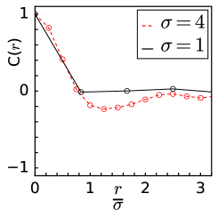
where $\gamma(\vec{r})=J_{1}({|\vec{r}|}/\sigma)/({|\vec{r}|}/\sigma)$ with $J_{1}$ the first order Bessel function and $\sigma$ the speckle size (correlation length). Fig.1 shows the two point function generated on our finite lattice, for two $\sigma$ values. At large $\sigma$ the long distance behaviour of the correlation function deviates from the ideal form on our $24\times 24$ lattice.

II.3 Monte Carlo strategy

The Hubbard interaction cannot be treated exactly so we follow the approach used in tarat1 . We write the partition function for the model as an imaginary time path integral:

$$Z = \int D(\overline{\psi},\psi)e^{-S[\overline{\psi},\psi]}$$ (4)

$$S = \int_{0}^{\beta}d\tau[\sum\limits_{i,\sigma}\overline{\psi}_{i,\sigma}\partial_{\tau}\psi_{i,\sigma}+H(\psi,{\bar{\psi}})]$$

The $\psi_{i}(\tau)$ are Grassmann fields. The quartic term in the action prevents exact evaluation of $Z$. To proceed it is usual to introduce auxiliary fields to ‘decouple’ the interaction. This Hubbard$-$Stratonovich transformation, in terms of (a) a complex scalar ‘pairing field’ $\Delta_{i}=|\Delta_{i}|e^{i\theta_{i}}$, and (b) a a real scalar field $\phi_{i}$, is accomplished by writing:

$$exp(U\int d\tau{\bar{\psi}}_{i\uparrow}(\tau){\psi}_{i\uparrow}(\tau){\bar{\psi}}_{i\downarrow}(\tau){\psi}_{i\downarrow}(\tau))$$ (5)

$$~{}~{}~{}~{}~{}~{}~{}~{}~{}~{}~{}~{}~{}~{}~{}~{}~{}~{}~{}~{}~{}~{}~{}~{}~{}~{}~{}~{}~{}~{}~{}~{}~{}~{}~{}~{}~{}~{}~{}~{}~{}~{}~{}~{}~{}~{}~{}~{}~{}~{}~{}~{}~{}~{}~{}~{}~{}~{}~{}=\int d{\Delta}_{i}d{\Delta}^{*}_{i}d\phi_{i}e^{-S_{HS}}$$ (6)

$$S_{HS}=\int d\tau[\rho_{i}\phi_{i}+(\psi_{i\uparrow}\psi_{i\downarrow}\Delta_{i}+h.c)+{1\over U}(|\Delta_{i}(\tau)|^{2}+\phi_{i}^{2})]$$

The action is now quadratic in the fermions. Quantum Monte Carlo (QMC) proceeds to sample the fields $\Delta_{i}(\tau),\phi_{i}(\tau)$, or their Matsubara components $\Delta_{i}(i\Omega_{n}),\phi_{i}(i\Omega_{n})$. We employ a ‘static path approximation’ (SPA) wherein these fields are assumed to be ‘$\tau$ independent’ (or, alternately, having only a $\Omega_{n}=0$ component), but fluctuating spatially. The SPA approach retains all the classical amplitude and phase fluctuations in the model and has been elaborately benchmarked in the BCS-BEC crossover problem. We show its match with QMC in the discussion section.

When the auxiliary fields are assumed to be static, $Z$ becomes:

$$Z~{}~{}~{} = ~{}\int{\cal D}\Delta{\cal D}\Delta^{*}{\cal D}\phi~{}Tr[e^{-\beta H_{eff}}]$$ (7)

$$H_{eff}~{} = H_{0}+H_{coup}+{1\over|U|}\sum\limits_{i}(|\Delta_{i}|^{2}+\phi_{i}^{2})$$ (8)

$$H_{0}~{}~{}~{} = -t\sum_{<ij>}^{\sigma}c^{\dagger}_{i\sigma}c_{j\sigma}+\sum\limits_{i\sigma}(V_{i}-{\mu})n_{i\sigma}$$ (9)

$$H_{coup} = ~{}~{}\sum_{i}(\Delta_{i}c^{\dagger}_{i\uparrow}c^{\dagger}_{i\downarrow}+h.c)+\sum_{i}\phi_{i}n_{i}$$

This is a model of quadratic fermions coupled to classical fields. The Boltzmann weight for the fields can be inferred from the top equation: $e^{-\beta H(\Delta,\Delta^{*},\phi)}\propto~{}Tr[e^{-\beta H_{eff}}]$. The strategy, like in QMC, would be to pick the auxiliary fields following their Boltzmann weight, solve the corresponding fermion problem, and average over configurations.

Consider the $T=0$ and the finite $T$ cases separately. (i) As $T\rightarrow 0$, the system is pushed towards the maximum probability configuration, i.e, the minimum of $H(\Delta,\Delta^{*},\phi)$. The conditions, ${\partial H}/{\partial\Delta_{i}}=0$, ${\partial H}/{\partial\phi_{i}}=0$, etc, define the usual mean field HFBdG ground state. (ii) At $T\neq 0$, the fields fluctuate and we generate the equilibrium $\{\Delta_{i},\phi_{i}\}$ configurations by using a Metropolis algorithm. For each attempted update of the $\Delta_{i},\phi_{i}$ we diagonalise the fermionic problem on a $8\times 8$ cluster around the update site and compute the energy cost of the move tca .

II.4 Indicators

We keep track of the following:

1. The ${\bf q}=(0,0)$ component of the pairing field structure factor,

   $$S({\bf q})={1\over N^{2}}\sum_{ij}\langle\Delta^{\ast}_{i}\Delta_{j}\rangle e^{i{\bf q}.(\vec{r}_{i}-\vec{r}_{j})}$$

   both to determine the presence of superfluidity and also to locate the $T_{c}$ scale. Angular brackets indicate thermal average.

2. The overall density of states:

   $$~{}~{}N(\omega)=\frac{1}{N}\sum_{n}\langle|u_{n}|^{2}\delta(\omega-E_{n})+|v_{n}|^{2}\delta(\omega+E_{n})\rangle$$

   The $u_{n}$ and $v_{n}$ are components of the HFBdG eigenfunctions, and $E_{n}$ are the eigenvalues, in individual equilibrium $(\Delta_{i},\phi_{i})$ configurations. Since the configurations arise following a Boltzmann weight, thermal average is same as average over equilibrium configurations.

3. Localisation effects are tracked via the inverse participation ratio. For a normalised state $|n\rangle$, the inverse participation ratio (IPR) is $P(n)=\sum_{i}|\langle i|n\rangle|^{4}$. Averaged over an energy interval this leads to:

   $$P(\omega)={1\over N(\omega)}\sum_{n}\delta(\omega-\epsilon_{n})P(n)$$

   $P(\omega)$ is a inverse measure of the number of sites over which eigenstates at energy $\omega$ are spread.

Figure 2: Maps for spatial patterns in the ground state. The top row shows the disorder potential $V_{i}$ for fixed $V$ and four speckle sizes $\sigma$. Patterns for different $V$ can be generated by simply scaling these up. Notice the more random $V_{i}$ landscape at small $\sigma$ and the progressively smoother variation at larger $\sigma$. The lower set of panels shows the amplitude $|\Delta_{i}|$ for varying $V$ and $\sigma$. From the top row down $V=0.5t,~{}1.5t,~{}2.5t$. The small $V$ large $\sigma$ pattern has the strongest order while the large $V$ small $\sigma$ panel has the weakest order. Spatially, $|\Delta_{i}|$ anti-correlates with the extremes in $V_{i}$.

III Ground state

The ground state of disordered superfluids is characterised by two spatially varying averages, $\langle n_{i}\rangle$ and $\langle c^{\dagger}_{i\uparrow}c^{\dagger}_{i\downarrow}\rangle$. They are related, in our approach, to the fields $\phi_{i}$ and $\Delta_{i}$. At $T=0$ within our scheme (and mean field theory) the phase $\theta_{i}$ is same at every site. Let us start with the spatial behaviour.

III.1 Spatial behaviour

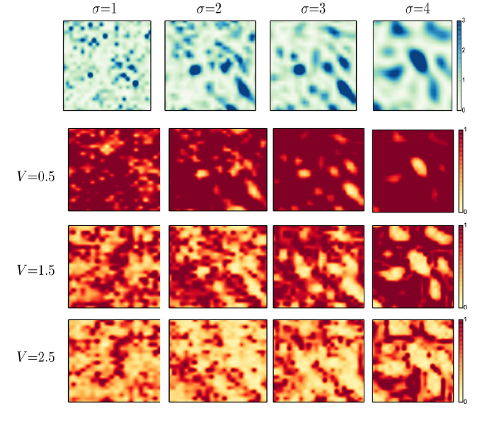
Fig.2 shows the spatial behaviour in the ground state for changing speckle size and disorder strength. The top row shows the pattern of the bare disorder $V_{i}$ for fixed $V$ and four speckle sizes. Realisations with larger $V$, but same $\sigma$, can be generated by simply scaling the potential in the top row.

As expected, the $V_{i}$ shows a rapid site to site variation at $\sigma=1$ and a progressively smoother, island like structure, at $\sigma=4$. The lower set of panels shows the amplitude, $|\Delta_{i}|$, of the pairing field that emerges for different combinations of $V$ and $\sigma$. The $V$ values are chosen to capture behaviour at weak disorder $(V=0.5t)$, close to critical $(V=1.5t)$, and in the insulating regime $(V=2.5t)$ in the uncorrelated limit. Expectedly, the $|\Delta_{i}|$ is large and quasi homogeneous at small $V$ and large $\sigma$ (top right) and rapidly varying and of small average value when $V$ is large and $\sigma$ is small (bottom left). The $|\Delta_{i}|$ also ‘anti correlates’ with the extremes $V_{i}$, since these regions - with $n_{i}$ close to $0$ or $2$ - suppress charge fluctuation.

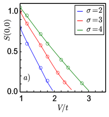
While it seems that an increase in $V$ can be ‘compensated’ by an increase in $\sigma$, to retain the same degree of overall order, the situation is more subtle. From Fig.3(a) we located $(V,\sigma)$ pairs where the overall magnitude of the order is same at $T=0$. The pair ($V=1.5t,\sigma=2$) and ($V=2.5t,\sigma=4$) above satisfy this. Spatial similarity? The small $V$ small $\sigma$ pattern, while inhomogeneous, has a more ‘space filling’ character in the order parameter compared to the large $V$ large $\sigma$ case where a small fraction of the total area has large $\Delta_{i}$ and large areas have $\Delta_{i}\rightarrow 0$. The large hills and valleys created by the strong $V$ large $\sigma$ make the $\Delta_{i}$ pattern more filamentary. An increase in $\sigma$ is not simply like a decrease in $V$.

III.2 Phase diagram

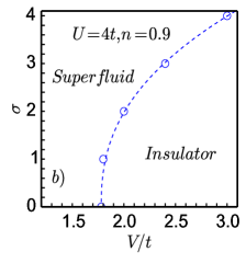
While the local distribution follows $P(v)\propto e^{-v/V}$, the introduction of a correlation length $\sigma$ makes the critical disorder $V_{c}$ dependent on $\sigma$. Fig.3(a) shows how the SF order parameter at $T=0$ (obtained by extrapolating the finite $T$ result) falls with $V/t$ for different $\sigma$. The intersection of these lines with the $x$ axis maps out $V_{c}(\sigma)$.

Fig.3.(b) shows the $V-\sigma$ ground state phase diagram obtained by the method above. For uncorrelated exponential disorder we find $V_{c}\sim 1.8t$. With increase in $\sigma$ the $V_{c}$ increases - widening the SF window - and we find that $V_{c}(\sigma)-V_{c}(0)\propto\sigma^{\alpha}$ with $\alpha\sim 2.4$. We call the phase without SF order an ‘insulator’ since it has an interaction induced gap in the spectrum.

Figure 3: Order in the ground state: (a). The superfluid order parameter, i.e, the pairing field structure factor $S({\bf q}=(0,0))$, extrapolated down to $T=0$, as a function of disorder strength $V$ at various speckle size $\sigma$. The critical disorder for SF to insulator transition increases with $\sigma$. (b) The ground state phase diagram at $U=4t$ and $n=0.9$ that emerges from the data in panel (a). The dotted line is a fit $V_{c}(\sigma)-V_{c}(0)\propto\sigma^{2.4}$.

Figure 4: Density of states in the ground state. Panels (a)-(c) show the DOS at three strengths of disorder $V$ and for four $\sigma$ at each $V$. Increase in $\sigma$ sharpens the coherence peak but also suppresses the gap. Panels (d)-(f) show the same data as in (a)-(c) now highlighting the variation with $V$ at fixed $\sigma$. Here increasing $V$ suppresses both the coherence peak and the gap.

III.3 Density of states

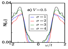
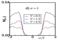
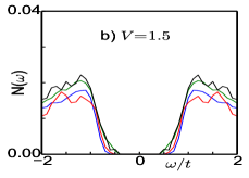
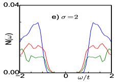
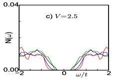
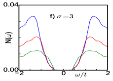
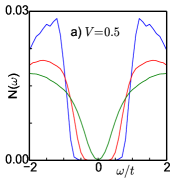
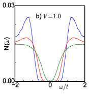
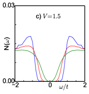
We now examine the DOS in the ground state for varying $V$ and $\sigma$, Fig.4. The left column shows results at fixed $V$, while the right column shows the same data organised in terms of fixed $\sigma$. Panel (a) shows the $\sigma$ dependence at weak disorder. There are three effects that emerge on increasing $\sigma$: (i) the ‘coherence peak’ sharpens, (ii) the gap in the DOS reduces, and (iii) the rise from the gap edge to the coherence peak shows a reducing slope - unlike the sharp rise that one sees in a clean system. Panels (b) and (c) show behaviour similar to (a) except for an overall suppression in magnitude (the bandwidths are much larger here) and a rather tenuous coherence feature.

Figure 5: Variation of the superfluid $T_{c}$ with disorder and speckle correlation length. (a) Disorder dependence for various $\sigma$. At $V=0$ we have the ‘clean’ $T_{c}$. The rate of fall with $V$ decreases with increasing $\sigma$. (b) Firm lines: $T_{c}$ for varying $\sigma$ and three values of $V$. Dotted lines: $T_{g}$ - low $T$ gap to high $T$ pseudogap crossover temperature.

Figure 6: Speckle size and temperature dependence of $\Delta_{0}.\Delta_{i}$ at strong disorder. $\Delta_{0}$ is the pairing field at a reference (corner) site. The overlap is based on a single MC configuration at $V=2t$ and the $\sigma,T$ indicated. Increasing $\sigma$ augments intersite correlation, with the largest $\sigma$ lowest $T$ panel (top right) having the strongest correlation. Bottom row: Density of states at $V=2t$, showing $\sigma$ and $T$ dependence. At low $\sigma$ the low $T$ state shows no coherence peak, and a broad gap that smears out with increasing $T$. At $\sigma=4$ there is a reasonable coherence feature, and a smaller gap at low $T$. The gap fills more quickly with rising $T$ than at $\sigma=1$. The behaviour in panels (b)-(c) interpolate between (a) and (d).

Feature (i) above would be expected also in terms of a decrease in the effective disorder, (ii) and (iii) however contradict that interpretation. As we will see, an increase in $\sigma$ does not make the $|\Delta_{i}|$ large and homogeneous, it makes the $|\Delta_{i}|$ distribution very broad, with large weight at small $|\Delta|$. This leads to the low energy weight and unusual shape in $N(\omega)$.

The disorder dependence at fixed $\sigma$ is more traditional. Increasing $V$ suppresses the coherence peak and increases low energy spectral weight - effectively reducing the gap. The feature is visible in panels (d)-(f).

IV Thermal fluctuations

To understand how speckle correlations affect the $T_{c}$ and spectral properties we do a Monte Carlo on $H_{eff}$, annealing the variables $\phi_{i}$ and $\Delta_{i}$, which now pick up a distribution at each site. We compute spatial correlations and DOS averaged over equilibrium configurations.

IV.1 Phase diagram

Tracking the ordering peak, $S({\bf q}=0)$ in the pairing structure factor allows us to locate a transition scale. For our density and interaction choice that scale is $\sim 0.13t$ in the clean limit. We choose several $V$ for $\sigma=1-4$, and about 10 realisations for each $(V,\sigma)$ combination, and cool the system from high temperature. We save equilibrium configurations of $\{\Delta_{i},\phi_{i}\}$, the pairing structure factor $S({\bf q})$, and the DOS.

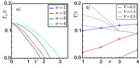
The $T_{c}$ scale that emerges is shown in Fig.5. Panel (a) shows the $V$ dependence for different $\sigma$ while panel (b) shows the $\sigma$ dependence at fixed $V$. In (a) all the $T_{c}$ curves start at the clean value when $V=0$. The drop with $V/t$ is relatively quick at $\sigma=1$, hitting $T_{c}=0$ at $V\sim 1.8t$, while at $\sigma=4$ the fall is much slower and the critical disorder is $V\sim 3t$. These numbers lead to the phase diagram in Fig.3.

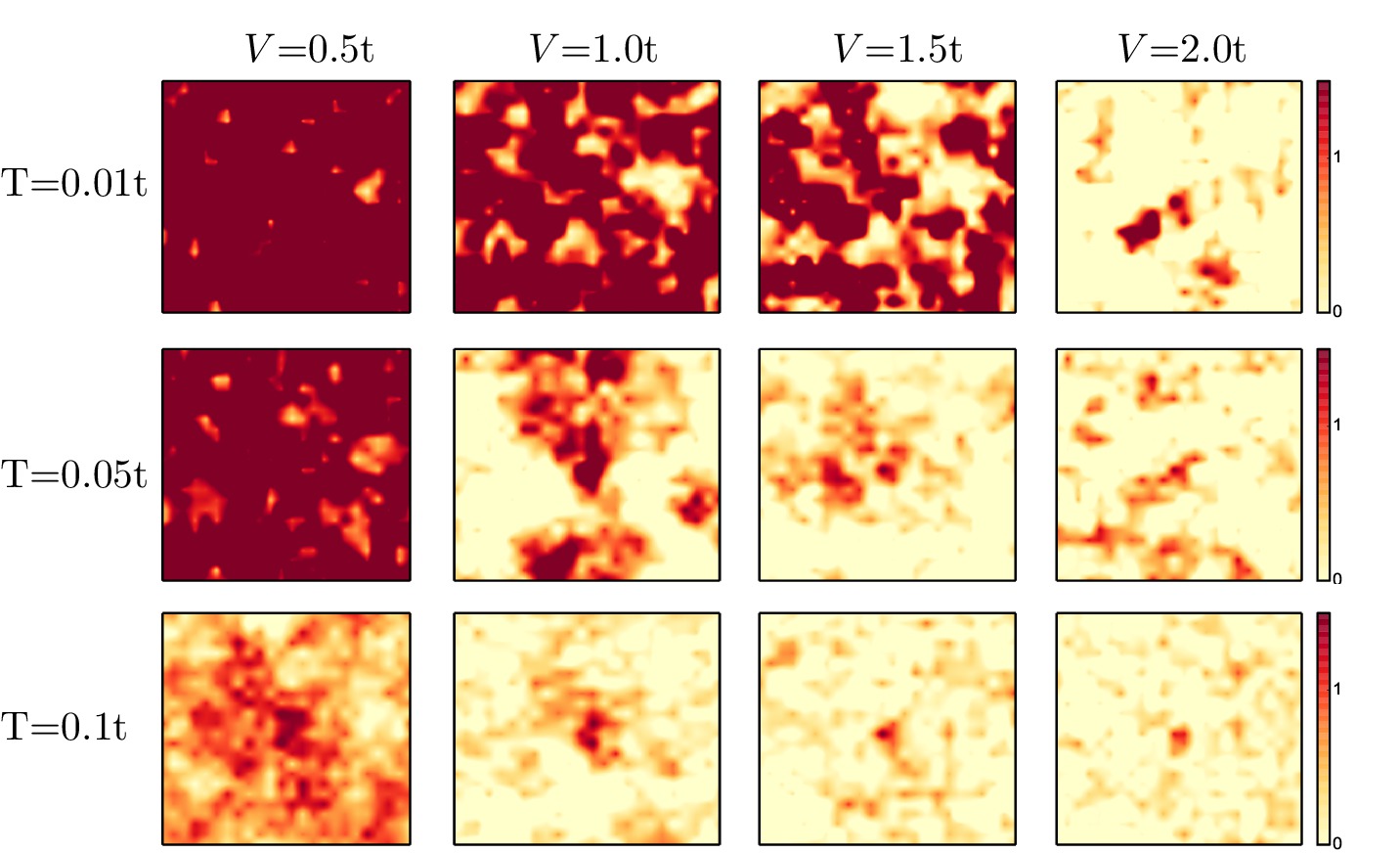
Panel (b) shows the effect of increasing $\sigma$ on the $T_{c}$, for fixed values of $V$. At weak disorder, $V=0.5t$, the $T_{c}$ rises slowly with increasing $\sigma$ and tends to reach the clean limit value for $\sigma\gtrsim 4$. At $V=1.5t$, where for uncorrelated disorder the system is close to a SF-insulator transition, increasing $\sigma$ leads to a quicker rise in $T_{c}$. The third case, at $V=2.5t$ is the most interesting. Here the system remains insulating upto $\sigma\sim 3$ and only at $\sigma=4$ do we see a small finite $T_{c}$. This is a speckle size induced insulator to SF transition - the bottom right panel in Fig.2 suggests that this occurs via percolation. The dotted lines indicate a crossover from the low $T$ ‘gapped’ regime to a higher $T$ pseudogap regime. The corresponding $T_{g}$ scale reduces with increasing $\sigma$.

   

Figure 7: Disorder and temperature dependence of $\Delta_{0}.\Delta_{i}$ at moderate speckle size, $\sigma=2$. At fixed temperature along the row the correlation decreases with increase in $V$. The correlation is strongest at $V=0.5t$ and $T=0.01t$ and decreases with increasing $V$ or $T$. Bottom row: DOS at $\sigma=2$, showing $V$ and $T$ dependence. The suppression in coherence peak is seen with increasing temperature and disorder strength. The gap in the density of states reduces with increasing temperature. This effect is more pronounced at small disorder strength.

IV.2 Variation in speckle size

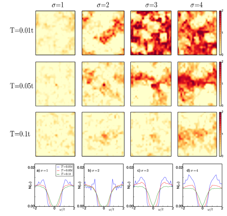
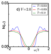
Fig.6 shows the spatial correlations of the pairing field at $V=2t$ (where the uncorrelated disorder problem would be insulating) for four speckle sizes and three temperatures. To keep track of both amplitude and phase correlations we plot the scalar $C_{i}={\Delta}_{0}.{\Delta}_{i}$, where ${\vec{R}}_{0}$ is a reference (corner) site and ${\vec{R}}_{i}$ is the site under consideration, treating $\Delta$ like a two dimensional ‘vector’. At the lowest $T$ there is hardly any pairing correlation at $\sigma=1$, some trace at $\sigma=2$, and percolative patterns at $\sigma=3-4$. Naturally the finite $T$ systems at $\sigma=1,2$ do not have any SF correlations, the $\sigma=3$ system seems to lose global correlation at $T<0.05t$, while the $\sigma=4$ system loses its order somewhere between $T=0.05t$ and $T=0.1t$. One can draw a $T_{c}(\sigma)$ plot akin to Fig.5(b) that shows the onset of SF order for $\sigma>2$ and a gradual enhancement of $T_{c}$ with $\sigma$. With increase in $\sigma$ the low $T$ gap in the DOS reduces while the coherence peak sharpens. Increase in $T$ leads to a quicker closure of the gap in the large $\sigma$ system.

IV.3 Variation in disorder strength

Fig.7 shows data that is complementary to Fig.6, now focusing on results at a fixed speckle size $\sigma=2$. As expected the low $T$ system shows SF order for $V\lesssim 1.5t$ and insulating character for $V=2t$. The $V=2t$ system continues to remain insulating at all $T$ while the weaker disorder cases show a fragmentation of the spatial order, and its loss at a scale $T_{c}(V)$, with increasing $T$. The associated $T_{c}$ are given in Fig.5(a).

The change in DOS with $V$ and $T$ is as anticipated. At low $V$ the low $T$ DOS has a large gap with sharp edge and reasonable coherence peaks. With increasing $T$ there is a transfer of weight to low energy and a smearing of the coherence feature. With increase in $V$ the low $T$ DOS shows a smaller gap and for $V\gtrsim 1.5t$ no coherence peaks are visible. However, the transfer of spectral weight to low frequency, due to increasing $T$, is weaker in the larger $V$ case compared to weak disorder.

Figure 8: Maps for the effective potential $V_{eff}$ for varying speckle size and disorder strength. The disorder is $V=0.5t,~{}1.5t,~{}2.5t$ from top to bottom, while the speckle size is $\sigma=1,~{}2,~{}3,~{}4$ from left to right. The bottom left panel - large $V$ and small $\sigma$ - has the most fluctuating pattern while the top right panel - small $V$ and large $\sigma$ - has the smoothest profile.

V Discussion

Having seen the results of increasing speckle size on the ground state and thermal properties of the superfluid, we want to suggest how these effects arise from the renormalised effective potential that emerges in this problem.

V.1 Understanding the ground state

V.1.1 Nature of the effective disorder

From previous studies on uncorrelated disorderghosal-prb we know that the presence of the Hartee term in HFBdG Hamiltonian enhances the effect of disorder. At $U\gg t$ and in the presence of disorder the density field become strongly inhomogeneous due to the Hartree feedback from the interaction term. As a result, the effective potential to which the fermions react is not $V_{i}$ but $V_{eff}=V_{i}+\phi_{i}=V_{i}+{U\over 2}\langle n_{i}\rangle.$ In contrast to a weakly interacting system with uncorrelated disorder the pairing in the present problem would involve fermions in an effective potential that is (i) strongly renormalised due to the large $U$, and (ii) spatially correlated due to the fermionic feedback and finite $\sigma$. The combination of $V$ and $U$ enhances localisation, while increasing $\sigma$ at fixed $(V,U)$ weakens localisation. These effects in turn impact on the phase stiffness which dictates the $T_{c}$ scales of the superfluid tarat-arx .

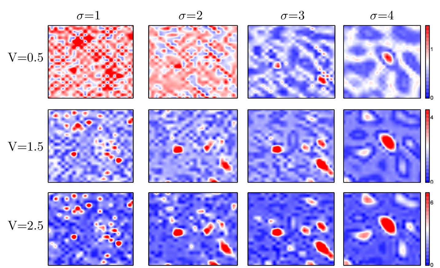
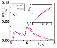
With this in mind, Fig.8 shows maps of the effective potential $V_{eff}$ for varying $V$ and $\sigma$. The $\phi$ that enters $V_{eff}$ is obtained via the full HFBdG minimisation. As expected the $V_{eff}$ at small $\sigma$ is rapidly fluctuating while at large $\sigma$ the variation is much smoother. The main impact of $\phi_{i}$ is to increase the width of the effective disorder leaving the spatial correlation more or less as in $V_{i}$. This is borne out by comparing Fig.8 with the top row in Fig.2.

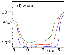
We show the distribution of $V_{eff}$ at three values of $V$ in Fig.9(a)-(c), comparing results at $\sigma=1$ and $\sigma=4$. The distributions show marginally greater weight at large $V_{eff}$ for the larger $\sigma$ case.The inset of Fig.9(c) compares the standard deviation $\delta V_{eff}=\sqrt{\braket{V_{eff}(\vec{r})^{2}}-\braket{V_{eff}(\vec{r})}^{2}}$ for two values of $\sigma$. The $\delta V_{eff}$ at $\sigma=4$ is only slightly larger than that at $\sigma=1$. We conclude that the local distribution of $V_{eff}$ is mainly independent of speckle size.

   

 

Figure 9: (a)-(c) shows $P(V_{eff})$ at $V=0.5t,1.5t,2.5$, respectively, comparing $\sigma=1$ with $\sigma=4$. Inset of Panel (c) shows the variance $\delta V_{eff}$ with respect to $V$ at $\sigma=1,4$. At a given $V$ the variance is slightly larger at $\sigma=4$ compared to $\sigma=1$. (d) The normalised $C(\vec{r})$ as a function of disorder for two speckle sizes. The behaviour suggests that the spatial correlation in $V_{eff}$ is dictated by just $\sigma$ and is unaffected $V$.

Figure 10: The distribution of $|\Delta_{i}|$ in the ground state comparing the $\sigma$ dependence at $V=0.5t,1.5t,2.5t$. At larger $V$ the effect of $\sigma$ is to create a distribution with large weight at low amplitude.

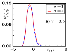
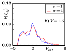
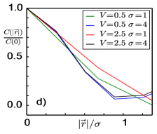
To characterise the spatial correlations in $V_{eff}$ panels 9(d) show the plot of

$$C(|\vec{r}|)=\braket{V_{eff}(\vec{x}+\vec{r})V_{eff}(\vec{x})}-\braket{V_{eff}(\vec{x})}^{2}$$

for speckle sizes 1 and 4. These indicate that the spatial correlations depend on $\sigma$ but are essentially $V$ independent. Overall, Fig.9 suggests that the strength of $V_{eff}$ is dictated by $V$ and $U$ while the correlations in $V_{eff}$ are dictated by $\sigma$ only.

 

Figure 11: DOS and IPR in the background of the bare disorder, $V_{i}$. The DOS naturally broadens with $V$ but is not very sensitive to $\sigma$. The IPR however is sensitive to $\sigma$ and shows weaker localisation (smaller IPR) at larger $\sigma$.

Figure 12: DOS and IPR in the presence of the effective disorder $V_{i}^{eff}=V_{i}+\phi_{i}$. We have ignored the pairing effects in this calculation. The $V_{i}^{eff}$ problem has larger bandwidth, due to the larger effective disorder, and greater localisation compared to the bare disorder. The IPR is much larger than in the $V_{i}$ problem, and much larger at $\sigma=1$ compared to $\sigma=4$.

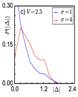
V.1.2 Order parameter in the ground state

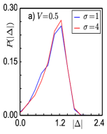
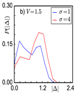
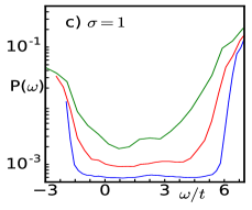
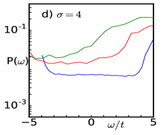
Fig.10 shows the distribution of $|\Delta_{i}|$ in the ground state for three values of $V$ and two speckle size. While $\sigma$ has little effect in the distribution at $V=0.5t$, there is a distinct $\sigma$ dependence at larger disorder - for a given $V$ the distribution at larger $\sigma$ has much greater weight at low amplitude. This correlates with the behaviour of the spatial patterns and the DOS that we have seen earlier.

V.1.3 Localisation effects

While the $V_{eff}$ and the resulting $\Delta_{i}$ control features like the DOS, to understand intersite coupling between the $\Delta_{i}$ we need to understand the spatial extent of the wavefunctions in the $V_{eff}$ background.

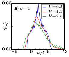
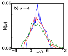
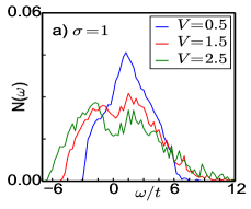
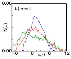
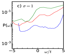
First the case of bare disorder, to set a reference. Fig.11 shows the DOS (upper row) and the IPR (lower row) in the presence of only $V_{i}$. The model is solved with $U$ set to zero. We show results for $V=0.5t,1.5t,2.5t$ and $\sigma=1,4$. Since $P(v)\sim e^{-v/V}$ has a finite positive mean the DOS and IPR plots are asymmetric about $\omega=0$. The greater width of the disorder distribution at larger $V$ leads to a correspondingly broader DOS. Comparing panels (a) and (b) the speckle size does not make a significant difference to the DOS. The IPR shows a more significant $\sigma$ dependence, particularly at large $V$. At $V=0.5t$ the IPR at the band center is $\ll 10^{-3}$, suggesting a localisation length $>\sqrt{10^{3}}$, larger than our system size $(24\times 24)$. At $V=2.5t$, however, there is a visible difference between the band center IPR at $\sigma=1$ and $\sigma=4$. Nevertheless the numbers for the IPR are still $\sim 10^{-3}$, indicating a large localisation length.

Fig.12 shows results on the DOS and IPR based on a $V_{eff}$ extracted from the solution of the HFBdG equation. The effective model that is solved to obtain the results in the figure is

$$H=-t\sum_{<ij>}c^{\dagger}_{i}c_{j}+\sum_{i}V^{eff}_{i}n_{i}$$

As in Fig.11 the disorder values are $0.5t,~{}1.5t,~{}2.5t$. The fermions are subject to a larger effective disorder than in Fig.11. As a result the weight spreads over a larger frequency window. Here again the the effect of disorder is somewhat weaker in (b) compared to (a).

The most interesting feature is the contrast between the IPR in Fig.11 with that in Fig.12. Note the following: (i) the IPR in the $V_{eff}$ problem, near $\omega=0$ or near the band edges, is at least an order of magnitude larger than the corresponding value in the bare disorder problem, and (ii) between Fig.12(c) and Fig.12(d) the larger $\sigma$ case shows a clearly smaller IPR. For example around $\omega=0$ the IPR at $V=2.5t$ and $\sigma=1$ is $\sim 2\times 10^{-1}$, while at $\sigma=4$ the corresponding IPR is $\sim 3\times 10^{-2}$. The associated ‘localisation length’ would be $\sim 2$ lattice spacings at $\sigma=1$ and $\sim 5$ lattice spacings at $\sigma=4$. These are well below our system size, and significantly different from one another. This feature of the single particle eigenfunctions enters the fermionic Green’s function $G_{ij}(i\omega_{n})$ and through that the phase stiffness and $T_{c}$ scales. We discuss this next.

V.2 Estimating the phase coupling and $T_{c}$ scales

To understand the intersite coupling between the pairing fields we derive an effective XY model and benchmark it with respect to full MC results. A study of the couplings $J_{ij}$ of this model with disorder and speckle size provides some insight on the phase transitions we observe in the parent problem. Postponing a detailed justification to the Appendix, the approximate model we use is of the form:

$$H_{XY} = -\sum_{ij}J_{ij}cos(\theta_{i}-\theta_{j})$$ (10)

$$J_{ij}~{} = ~{}J_{ij}^{0}\Delta_{i0}\Delta_{j0}$$ (11)

(12)

$$J_{ij}^{0}~{} = {1\over\beta}\sum_{n}[F_{ij}(i\omega_{n})F_{ji}(i\omega_{n})+G_{ij\uparrow}(i\omega_{n})G_{ij\downarrow}(-i\omega_{n})]$$

Figure 13: (a) The comparison of $T_{c}$ scales in the clean limit, between full QMC, our MC result (SPA) and the XY model in the text. We operate near the peak $T_{c}$, the BCS-BEC crossover regime. The SPA well approximates the QMC answer. The XY model also succeeds in capturing the non-monotonic dependence of $T_{c}$ on $U/t$. (b) Sum of nearest neighbour XY couplings versus sum of all couplings including nearest neighbour. For small to moderate $U$ the model has significant long range couplings and it is only at very large $U$ that it can be truncated to nearest neighbour.

Figure 14: Comaparison of $T_{c}$ scales obtained from exact MC with the XY model for two speckle sizes. Fig a) shows the comparison for speckle size 1 and Fig b) shows the comparison for speckle size 4. The difference in the results of the two calculation increases with decrease of disorder.

The $\Delta_{i0}$, etc, are the pairing field amplitude in the $T=0$ HFBdG state. $G_{ij}$ is the ‘normal’ Green’s function and $F_{ij}$ is the ‘anomalous’ Green’s function computed on the HFBdG state. Via these Green’s functions $J_{ij}$ contains information about excitations on the HFBdG ground state. Note that $J_{ij}$ is not limited to nearest neighbours.

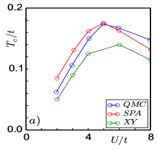
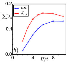
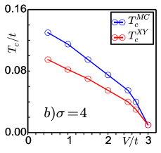
First a benchmark in the ‘clean’ problem. Fig.13(a) compares the $T_{c}$ scales obtained from the full MC with results from $H_{XY}$ as $U/t$ is varied across the BCS to BEC crossover. Given that no explicit finite temperature corrections have been included in the parameters of $H_{XY}$, the match is reasonable - and gets better at large $U$. Fig.13(b) focuses on the couplings that contribute to the $T_{c}$. At weak to intermediate coupling, in this clean limit, couplings beyond nearest neighbour have significant weight. This is demonstrated by the difference between the blue and red curves, for the NN coupling and the sum of all couplings, respectively. However when $U/t\gg 1$ the nearest neighbour coupling dominates.

Figure 15: Distribution of nearest neighbour bonds, averaged over the system and disorder configurations (a) $\sigma=1$ and (b) $\sigma=4$. With increase in disorder strength distribution becomes broad and peak of the distribution shifts to small values of $J_{nn}$. At the same disorder the peak is $P(J_{nn})$ is at a larger $J_{nn}$ at larger $\sigma$. This is the origin of the larger $T_{c}$.

At small $U$, one can drop the dependence of the $J_{ij}^{0}$ on the $\Delta_{i0}$ so the overall $J_{ij}\propto\Delta^{2}$. This vanishes as $U/t\rightarrow 0$. At large $U$, $J_{ij}^{0}\sim{1\over\Delta^{3}}$ so $J_{ij}\sim{1\over\Delta}\sim 1/U$ capturing the large $U$ asymptote. The model interpolates between the small $U$ and large $U$ limits.

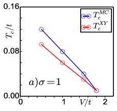
Now disorder. We use the approach above to compute $J_{ij}$. In presence of disorder effective $J_{ij}$ become inhomogeneous. Fig.14 compares the results of the full MC with that of $H_{XY}$ for two speckle sizes. There is a discrepancy at small disorder, traceable to the clean results at intermediate $U$, Fig.13 (we are working at $U=4t$), but the match improves at large disorder.

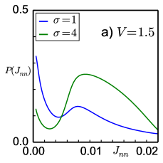
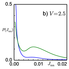
To understand the effect of disorder on the $J_{ij}$ we plot the distribution of nearest neighbour bond $J_{nn}$ for speckle sizes $\sigma=1,~{}4$ in Fig.15. At both $V=1.5t$ and $2.5t$ the $P(J)$ has a strong peak at low $J$ when $\sigma$ is small. By contrast most of the weight at large $\sigma$ is concentrated at intermediate $J$. The $P(J)$ forms an interesting counterpoint to the $P(|\Delta|)$ that we have seen before. The large $\sigma$ system has relatively smaller number of large $\Delta_{i}$ sites coupled strongly and - referring to the spatial maps - in a percolative pattern.

V.3 Connection to cold atomic experiments

To the extent we know, superfluidity of fermions in an optical lattice has not been observed yet, although superfluidity in the ‘continuum’, i.e, in a trap has been achieved. This is related to the lower $T_{c}$ (and entropy level) needed to achieve lattice superfluidity. Given this, there are no experiments yet that test out the effect of disorder, speckle or otherwise, on lattice Fermi superfluids. However, most of the qualitative features that we observe on increasing speckle size, e.g, the increase in $T_{c}$, the increase in low energy spectral weight, and the weakening localisation, are not lattice specific features. These effects should be visible in the continuum case as well.

Specifically, (i) The change in $T_{c}$ on increasing speckle size can be studied by tracking the condensate fraction via time of flight measurements. Such measurements are standard in clean superfluids and can be adapted to the disordered case 5 ; 6 ; 7 ; 8 . (ii) The suppression of the gap in the global DOS on increasing speckle size can be probed via radio frequency (RF) spectroscopy, already used in several cold atom experiments 9 ; 10 ; 12 . In fact there is now a proposal to measure the local DOS via an “energy-resolved atomic scanning probe” 16 . If such a method is implemented it would directly visualise the order parameter variation across the speckle disordered sample. (iii) Localisation effects in the disordered potential, and their weakening with increasing speckle size, can be probed via ‘expansion’ of the disordered gas on removing the trapping potentialexp-fermi-non-int0 ; exp-fermi-non-int1 . (iv) We did not consider transport effects since our degrees of freedom were supposed to be neutral (atoms). However, mass transport measurements in such disordered superfluids are already possible exp-fermi-int2 , and the impact of increasing speckle size at fixed disorder would be fascinating to observe.

VI Conclusion

We studied the speckle disorder driven superfluid-insulator transition for intermediate coupling fermions in a two dimensional lattice. The speckle disorder has an exponential on site distribution, and a correlation length $\sigma$. We observe the increase of the superfluid window at $T=0$, as well as increase in $T_{c}$, with increasing speckle size. In contrast to the disorder driven superfluid to insulator transition, which is well studied, we mapped out a speckle size driven insulator to superfluid transition. While some of the effects of increasing speckle size are crudely like a decrease in disorder, the underlying physics is more complex and contradicts this naive expectation.

Growing speckle size at strong disorder leads to an energy landscape with large scale undulations. In such a background the pairing amplitude is large only in a small fraction of sites. The small amplitude on the rest of the sites leads to suppression of the overall spectral gap, unlike what one would expect from an effective decrease in disorder. The smooth background leads to greater delocalisation of single particle states which generate an effective intersite coupling that grows with speckle size. This compensates for having fewer sites having a large $\Delta_{i}$ and leads to a higher $T_{c}$. The variation in the superfluid window with speckle size, the increase in $T_{c}$, and the unusual low energy spectral feature, are testable predictions from our work.

Acknowledgements: We acknowledge use of the HPC Clusters at HRI and thank Sauri Bhattacharyya for a reading of the manuscript. AJ thanks an Infosys grant for support.

Appendix A Derivation of the effective XY model

We outline here the derivation of effective model. The partition function of the fermion-auxiliary field model is given by

$$Z = \int D[\Delta,\Delta^{*}]D[\phi]D[\psi,\overline{\psi}]e^{-S_{eff}}$$ (13)

$$S_{eff} = \int_{0}^{\beta}d\tau[\sum\limits_{i,\sigma}\overline{\psi}_{i,\sigma}{\partial_{\tau}}\psi_{i,\sigma}+H_{eff}]$$ (14)

$$H_{eff}~{} = H_{0}+H_{coup}+{1\over|U|}\sum\limits_{i}(|\Delta_{i}|^{2}+\phi_{i}^{2})$$ (15)

$$H_{0}~{}~{}~{} = -t\sum_{<ij>}^{\sigma}{\bar{\psi}}_{i\sigma}\psi_{j\sigma}+\sum\limits_{i\sigma}(V_{i}-{\mu}){\bar{\psi}}_{i\sigma}{\psi}_{i\sigma}$$ (16)

$$H_{coup} = ~{}~{}~{}~{}\sum_{i}(\Delta_{i}{\bar{\psi}}_{i\uparrow}{\bar{\psi}}_{i\downarrow}+h.c)+\sum_{i}\phi_{i}\rho_{i}$$

Now we approximate $\phi_{i}=\phi_{0,i}$ where $\phi_{0i}$ is the $T=0$ saddle point value of $\phi$ field and similarly we approximate $\Delta_{i}=\Delta_{0i}+\delta\Delta_{i}$ where $\Delta_{0i}$ is the $T=0$ saddle point value of $\Delta$ field. $S_{eff}$ can be rewritten as

$$S_{eff} \approx S_{1}+S_{2}+S_{3}+S_{4}$$ (17)

$$S_{1} = \int_{0}^{\beta}d\tau\sum\limits_{i,\sigma}\overline{\psi}_{i,\sigma}({\partial_{\tau}}-\mu)\psi_{i,\sigma}+\sum_{i}(\Delta_{0i}\overline{\psi}_{i\uparrow}\overline{\psi}_{i\downarrow}+h.c)$$ (18)

$$+ \sum_{i}\phi_{0i}n_{i}+H_{0i}+{1\over|U|}\sum\limits_{i}(|\Delta_{0i}|^{2}+\phi_{0i}^{2})$$ (19)

$$S_{2} = \int_{0}^{\beta}\sum_{i}(\delta\Delta_{i}\overline{\psi}_{i\uparrow}\overline{\psi}_{i\downarrow}+h.c)$$ (20)

$$S_{3} = {\beta\over|U|}\sum\limits_{i}(\delta\Delta^{*}_{i}\Delta_{0i}+\delta\Delta_{i}\Delta_{0i}^{*})$$ (21)

$$S_{4} = {\beta\over|U|}\sum\limits_{i}\delta\Delta^{*}_{i}\delta\Delta_{i}$$

The original partition function is approximated by

$$Z\approx\int D[\delta\Delta,\delta\Delta^{*}]D[{\psi},\overline{{\psi}}]e^{-S_{1}-S_{3}-S_{4}}(\sum\limits_{n}{(-S_{2})^{n}\over n!})$$ (22)

$$= \int D[\delta\Delta,\delta\Delta^{*}]D[{\psi},\overline{{\psi}}]e^{-S_{1}-S_{3}-S_{4}}(1-S_{2}+{(S_{2})^{2}\over 2!}+...)$$

$$= \int D[\delta\Delta,\delta\Delta^{*}]Tr[e^{-\beta H_{f}}]e^{-S_{3}-S_{4}}(1-\braket{S_{2}}+{\braket{S_{2}^{2}}\over 2!}+...)$$

where

$\int D[c,\overline{c}]e^{-S_{1}}=Tr[e^{-\beta H_{f}}]$

$$H_{f} = H_{0}+\sum_{i}((\Delta_{0i}c^{\dagger}_{i\uparrow}c^{\dagger}_{i\downarrow}+h.c)+\phi_{0i}n_{i})$$ (24)

$$+{1\over|U|}\sum\limits_{i}(|\Delta_{0i}|^{2}+\phi_{0i}^{2})$$

Now

$$\int D[c,\overline{c}]e^{-S_{1}}S_{2} = \braket{S_{2}}$$ (25)

$$S_{3}-\braket{S_{2}} = 0$$

$$Z\approx\int D[\delta\Delta,\delta\Delta^{*}]Tr[e^{-\beta H_{f}}]e^{-S_{4}}(1+{\braket{S_{2}^{2}}-\braket{S_{2}}^{2}\over 2!}+...)$$

$${\braket{S_{2}^{2}}-\braket{S_{2}}^{2}\over 2!}={1\over 2!}\int_{0}^{\beta}d\tau_{1}d\tau_{2}\sum_{ij}X_{ij}(\tau_{1},\tau_{2})$$

$$X_{ij}(\tau_{1},\tau_{2}) = -\delta\Delta_{i}\delta\Delta_{j}F_{ij}(\tau_{1}-\tau_{2})F_{ji}(\tau_{2}-\tau_{1})$$

$$-\delta\Delta_{i}^{*}\delta\Delta_{j}^{*}F_{ji}(\tau_{1}-\tau_{2})F_{ij}(\tau_{2}-\tau_{1})$$

$$+\delta\Delta_{i}^{*}\delta\Delta_{j}G_{ij\uparrow}(\tau_{1}-\tau_{2})G_{ij\downarrow}(\tau_{1}-\tau_{2})$$

$$+\delta\Delta_{i}\delta\Delta_{j}^{*}G_{ji\downarrow}(\tau_{2}-\tau_{1})G_{ji\uparrow}(\tau_{2}-\tau_{1})$$

$F_{ij}(\tau_{2}-\tau_{1}))=Tr[e^{-\beta H_{eff}}T_{\tau}c^{\dagger}_{i\uparrow}(\tau_{2})c^{\dagger}_{j\downarrow}(\tau_{1})]/Tr[e^{-\beta H_{eff}}]$

$G_{ij\sigma}(\tau_{2}-\tau_{1}))=Tr[e^{-\beta H_{eff}}T_{\tau}c_{i\sigma}(\tau_{2})c^{\dagger}_{j\sigma}(\tau_{1})]/Tr[e^{-\beta H_{eff}}]$

Let’s assume small angular fluctuations $\delta\Delta_{i}=\iota\theta\Delta_{0i}$

${\braket{S_{2}^{2}}-\braket{S_{2}}^{2}\over 2!}=\beta\sum\limits_{ij}\theta_{i}\theta_{j}\Delta_{0i}\Delta_{0j}J_{ij}$

$J_{ij}^{0}={1\over\beta}\sum\limits_{n}[F_{ij}(\iota\omega_{n})F_{ji}(\iota\omega_{n})+G_{ij\uparrow}(\iota\omega_{n})G_{ij\downarrow}(-\iota\omega_{n})]$

$$J_{ij}^{0} = \sum\limits_{n1,n2}{(u_{n1}^{i*}v_{n1}^{j}u_{n2}^{i*}v_{n2}^{j}+v_{n1}^{i}u_{n1}^{j*}v_{n2}^{i}u_{n2}^{j*}\over E_{n1}+E_{n2}}$$

$$+{u_{n1}^{i}u_{n1}^{j*}u_{n2}^{i}u_{n2}^{j*}+v_{n1}^{i*}v_{n1}^{j}v_{n2}^{i*}v_{n2}^{j}\over E_{n1}+E_{n2}})$$

where $E_{n1}$ and $E_{n2}$ are eigenvalues and $u_{n}$ and $v_{n}$ are eigenvectors of HBDG problem in presence of $\Delta_{0i}$ and $\phi_{0i}$.

${\braket{S_{2}^{2}}-\braket{S_{2}}^{2}\over 2!}\approx-\beta\sum\limits_{ij}\Delta_{0i}\Delta_{0j}J_{ij}^{0}(1-\cos({\theta_{i}-\theta_{j}}))$

$$Z_{approx}\approx Tr[e^{-\beta H_{f}}]e^{-\beta\sum\limits_{ij}\Delta_{0i}\Delta_{0j}J_{ij}^{0}(1-\cos({\theta_{i}-\theta_{j}}))}$$

So the effective model for phase fluctuations over the ground state has the form:

$$H_{XY}=\sum\limits_{ij}\Delta_{0i}\Delta_{0j}J_{ij}^{0}(1-\cos({\theta_{i}-\theta_{j}}))$$

Subtracting a constant, this is the form used in the text.

References

- (1) P. W. Anderson, J. Phys. Chem. Solids 11, 26 195921.
- (2) A. A. Abrikosov and L. P. Gorkov, Zh. Eksp. Teor. Fiz. 36, 319 (1959).
- (3) E. Abrahams, P. W. Anderson, D. C. Licciardello, and T. V. Ramakrishnan, Phys. Rev. Lett. 42, 673 (1979).
- (4) For reviews, see A. M. Goldman and N. Markovic, Phys. Today 51, No 11, 39 (1998), D. Belitz and T. Kirkpatrick, Rev. Mod. Phys. 66, 261 (1994), M. V. Sadovskii, Phys. Rep. 282, 225 (1997), V. F. Gantmakher and V. T. Dolgopolov, Phys. Usp. 53, 3-53 (2010).
- (5) A. Ghosal, M. Randeria and N. Trivedi, Phy. Rev. B 65, 014501 (2001)
- (6) N. Trivedi, R. T. Scalettar and M. Randeria, Phys. Rev. B 54, 3756 (1996).
- (7) M. Mayr, G. Alvarez, C.Sen and E.Dagotto, Phys. Rev. Lett. 94, 217001 (2005).
- (8) Y. Dubi, Y. Meir and Y. Avishai, Nature, 449, 876 (2007).
- (9) K. Bouadim, Y. L. Loh, M. Randeria and N. Trivedi, Nature Phys. 7, 884 (2011)
- (10) D. B. Haviland, Y. Liu and A. M. Goldman, Phys. Rev. Lett. 62, 2180 (1989).
- (11) D. Shahar and Z. Ovadyahu, Phys. Rev. B 46, 10917 (1992).
- (12) W. Escoffier, C. Chapelier, N. Hadacek, and J.-C. Villégier, Phys. Rev. Lett. 93, 217005 (2004).
- (13) T. I. Baturina, A. Yu. Mironov, V. M. Vinokur, M. R. Baklanov, and C. Strunk, Phys. Rev. Lett. 99, 257003 (2007).
- (14) D. Jaksch, C. Bruder, J. I. Cirac, C. W. Gardiner, and P. Zoller, Phys. Rev. Lett. 81, 3108 (1998).
- (15) T. Esslinger, Annu. Rev. Condens. Matter Phys. 1, 129 (2010).
- (16) I. Bloch, Nature Phys. 1, 23 (2005).
- (17) A. Erez and Y. Meir, Phys. Rev. Lett. 111, 187002 (2013).
- (18) A. Erez and Y. Meir, Phys. Rev. B 88, 184510 (2013).
- (19) S. Tarat and P. Majumdar, Eur. Phys. J. B (2015) 88: 68
- (20) S. Tarat and P. Majumdar, Europhys. Lett. 105 (2014) 67002.
- (21) F. Palestini and G. C. Strinati, Phys. Rev. B 88, 174504 (2013)
- (22) R. C. Kuhn, C. Miniatura, D. Delande, O. Sigwarth and C. A. Muller, Phys. Rev. Lett. 95, 250403 (2005).
- (23) R. C. Kuhn, O. Sigwarth, C. Miniatura, D. Delande and C. A. Muller, New Journal of Physics 9 (2007) 161.
- (24) Serpil Sucu, Saban Aktas, S. Erol Okan, Zehra Akdeniz and Patrizia Vignolo, Phys. Rev. A84, 065602 (2011).
- (25) Marie Piraud, Luca Pezze and Laurent Sanchez-Palencia, Europhys. Lett., 99 (2012) 50003.
- (26) M Piraud, L Pezze and L Sanchez-Palencia, New Journal of Physics 15 (2013) 075007.
- (27) Dominique Delande and Giuliano Orso, Phys. Rev. Lett. 113, 060601 (2014).
- (28) E. Fratini and S. Pilati, Phys. Rev. A92, 063621 (2015).
- (29) W. Morong and B. DeMarco, Phys. Rev. A92, 023625 (2015).
- (30) Michael Pasek, Giuliano Orso, and Dominique Delande, Phys. Rev. Lett. 118, 170403 (2017).
- (31) F. Kruger, J. Wu, and P. Phillips, Phys. Rev. B 80, 094526 (2009).
- (32) U. Bissbort, R. Thomale, and W. Hofstetter, Phys. Rev. A 81, 063643 (2010).
- (33) S. Pilati, S. Giorgini, and N. Prokof’ev Phys. Rev. Lett. 102, 150402 (2009)
- (34) D. Semmler, J. Wernsdorfer, U. Bissbort, K. Byczuk, and W. Hofstetter, Phys. Rev. B82, 235115 (2010).
- (35) V. W. Scarola and B. DeMarco, Phys. Rev. A92, 053628 (2015).
- (36) S. Pilati and E. Fratini, Phys. Rev. A 93, 051604(R)(2016)
- (37) L. Sanchez-Palencia, D. Clement, P. Lugan, P. Bouyer, G. V. Shlyapnikov, and A. Aspect, Phys. Rev. Lett. 98, 210401 (2007).
- (38) Juliette Billy, Vincent Josse, Zhanchun Zuo, Alain Bernard, Ben Hambrecht, Pierre Lugan, David Clement, Laurent Sanchez-Palencia, Philippe Bouyer, Alain Aspect, Nature, Vol 453, 12 June 2008, 891.
- (39) Giacomo Roati, Chiara D’Errico, Leonardo Fallani, Marco Fattori, Chiara Fort, Matteo Zaccanti, Giovanni Modugno, Michele Modugno, Massimo Inguscio, Nature, Vol 453, 12 June 2008, 895.
- (40) F. Jendrzejewski, A. Bernard, K. Müller, P. Cheinet, V. Josse, M. Piraud, L. Pezze, L. Sanchez-Palencia, A. Aspect and P. Bouyer, Nature Phys, Vol 8, MAY 2012, 398.
- (41) L. Fallani, J. E. Lye, V. Guarrera, C. Fort, and M. Inguscio, Phys. Rev. Lett. 98, 130404 (2007).
- (42) M. White, M. Pasienski, D. McKay, S. Q. Zhou, D. Ceperley, and B. DeMarco, Phys. Rev. Lett. 102, 055301 (2009).
- (43) M. Pasienski, D. McKay, M. White, and B. DeMarco, Nature Phys, Vol 6, September 2010, 677.
- (44) S. S. Kondov, W. R. McGehee, J. J. Zirbel, B. DeMarco, Science 334, 66 (2011)
- (45) W. R. McGehee, S. S. Kondov, W. Xu, J. J. Zirbel, and B. DeMarco, Phys. Rev. Lett. 111, 145303 (2013).
- (46) S. S. Kondov, W. R. McGehee, W. Xu, and B. DeMarco, Phys. Rev. Lett. 114, 083002 (2015).
- (47) Sebastian Krinner, David Stadler, Jakob Meineke, Jean-Philippe Brantut, and Tilman Esslinger, Phys. Rev. Lett. 115, 045302 (2015).
- (48) Strictly speaking there is no superfluid-insulator transition at within the HFBdG scheme since quantum phase fluctuations are absent. However, at any small finite thermal fluctuations can cause a SIT.
- (49) S. Kumar and P. Majumdar, Eur. Phys. J. B, 50, 571 (2006).
- (50) S. Tarat and P. Majumdar, arXiv:1406.5423v1, supplementary material.
- (51) C. A. Regal, M. Greiner, D. S. Jin, Phys. Rev. Lett. 92, 040403 (2004)
- (52) M. W. Zwierlein, C. A. Stan, C. H. Schunck, S. M. F. Raupach, A. J. Kerman, and W. Ketterle , Phys. Rev. Lett. 92, 120403 (2004)
- (53) Qijin Chen, C. A. Regal, M. Greiner, D. S. Jin, and K. Levin, Phys. Rev. A 73, 041601(R) (2006)
- (54) Yasuhisa Inada, Munekazu Horikoshi, Shuta Nakajima, Makoto Kuwata-Gonokami, Masahito Ueda, and Takashi Mukaiyama, Phys. Rev. Lett. 101, 180406 (2008)
- (55) C. Chin, M. Bartenstein A. Altmeyer, S. Riedl, S. Jochim, J. Hecker Denschlag, R. Grimm , Science 305, 1128 (2004).
- (56) André Schirotzek, Yong-il Shin, Christian H. Schunck, and Wolfgang Ketterle, Phys. Rev. Lett. 101, 140403(2008)
- (57) Y. Shin, C. H. Schunck, A. Schirotzek, and W. Ketterle, Phys. Rev. Lett. 99, 090403 (2007)
- (58) D. Gruss, C.-C. Chien, M. Di Ventra, and M. Zwolak, New Journal of Physics 20, 115005 (2018)