Deep convolutional Gaussian processes
Abstract
We propose deep convolutional Gaussian processes, a deep Gaussian process architecture with convolutional structure. The model is a principled Bayesian framework for detecting hierarchical combinations of local features for image classification. We demonstrate greatly improved image classification performance compared to current Gaussian process approaches on the MNIST and CIFAR-10 datasets. In particular, we improve CIFAR-10 accuracy by over 10 percentage points.
1 Introduction
Gaussian processes (GPs) are a family of flexible function distributions defined by a kernel function (Rasmussen and Williams, 2006). The modeling capacity is determined by the chosen kernel. Standard stationary kernels lead to models that underperform in practice. Shallow – or single layer – Gaussian processes are often sub-optimal since flexible kernels that would account for non-stationary patterns and long-range interactions in the data are difficult to design and infer (Wilson et al., 2013; Remes et al., 2017). Deep Gaussian processes boost performance by modelling networks of GP nodes (Duvenaud et al., 2011; Sun et al., 2018) or by mapping inputs through multiple Gaussian process ’layers’ (Damianou and Lawrence, 2013; Salimbeni and Deisenroth, 2017). While more flexible and powerful than shallow GPs, deep Gaussian processes result in degenerate models if the individual GP layers are not invertible, which limits their potential (Duvenaud et al., 2014).
Convolutional neural networks (CNN) are a celebrated approach for image recognition tasks with superior performance (Mallat, 2016). These models encode a hierarchical translation-invariance assumption into the structure of the model by applying convolutions to extract increasingly complex patterns through the layers.
While neural networks have achieved unparalleled results on many tasks, they have their shortcomings. Effective neural networks require large number of parameters that require careful optimisation to prevent overfitting. Neural networks can often leverage a large number of training data to counteract this problem. Developing methods that are better regularized and can incorporate prior knowledge would allow us to deploy machine learning methods in domains where massive amounts of data is not available. Conventional neural networks do not provide reliable uncertainty estimates on predictions, which are important in many real world applications.
The deterministic CNN’s have been extended into the probabilistic domain with weight uncertainties (Blundell et al., 2015). Gal and Ghahramani (2016) explored the Bayesian connections of the dropout technique. Neural networks are known to converge to Gaussian processes at the limit of infinite layer width (MacKay, 1992; Williams, 1997; Lee et al., 2017). Garriga-Alonso et al. (2018) derive a kernel which is equivalent to residual CNNs with a certain prior over the weights. Wilson et al. (2016b) proposed a hybrid deep kernel learning approach, where a feature-extractor deep neural network is stacked with a Gaussian process predictor layer, learning the neural network weights by variational inference (Wilson et al., 2016a).
Recently Van der Wilk et al. (2017) proposed the first convolution-based Gaussian process for images with promising performance. They proposed a weighted additive model where Gaussian process responses over image subpatches are aggregated for image classification. The convolutional Gaussian process is unable to model pattern combinations due to its restriction to a single layer. Very recently Kumar et al. (2018) applied convolutional kernels in a deep Gaussian process, however they were unable to significantly improve upon the shallow convolutional GP model.
In this paper we propose a deep convolutional Gaussian process, which iteratively convolves several GP functions over the image. We learn multimodal probabilistic representations that encode combinations of increasingly complex pattern combinations as a function of depth. Our model is a fully Bayesian kernel method with no neural network component. On the CIFAR-10 dataset, deep convolutions increase the current state-of-the-art GP predictive accuracy from 65% to 76%. Our model demonstrates how a purely GP based approach can reach the performance of hybrid neural network GP models.
2 Background
In this section we provide an overview of the main methods our work relies upon. We consider supervised image classification problems with examples each associated with a label . We assume images as 3D tensors of size over channels, where RGB color images have color channels.
2.1 Discrete convolutions
A convolution as used in convolutional neural networks takes a signal, two dimensional in the case of an image, and a tensor valued filter to produce a new signal (Goodfellow et al., 2016). The filter is moved across the signal and at each step taking a dot product with the corresponding section in the signal. The resulting signal will have a high value where the signal is similar to the filter, zero where it’s orthogonal to the filter and a low value where it’s very different from the filter. A convolution of a two dimensional image and a convolutional filter is defined:
| (1) |
and is in . Here and define the size of the convolutional filter. Typical values could be or . Typically multiple convolutional filters are used, each convolved over the input to produce several output signals which are stacked together.
By default the convolution is defined over every location of the image. Sometimes one might use only every other location. This is referred to as the stride. A stride of 2 means only every other location is taken in the output.
2.2 Primer on Gaussian processes
Gaussian processes are a family of Bayesian models that characterize distributions of functions (Rasmussen, 2004). A zero-mean Gaussian process prior on latent function ,
| (2) |
defines a prior distribution over function values with mean and covariance:
| (3) | ||||
| (4) |
A GP prior defines that for any collection of inputs , the corresponding function values
follow a multivariate Normal distribution
| (5) |
is the kernel matrix encoding the function covariances. A key property of GPs is that output predictions and correlate according to the similarity of the inputs and as defined by the kernel .
Low-rank Gaussian process functions are constructed by augmenting the Gaussian process with a small number of inducing variables , and to obtain the Gaussian function posterior
| (6) |
where is the kernel between observed image pairs , the kernel is between observed images and inducing images , and kernel is between inducing images . (Snelson and Ghahramani, 2006)
2.3 Variational inference
Exact inference in a GP entails optimizing the evidence which has a limiting cubic complexity and is in general intractable. We tackle this restriction by applying stochastic variational inference (SVI) (Hensman et al., 2015a).
We define a variational approximation
| (7) | ||||
| (8) | ||||
with free variational parameters and a matrix to be optimised. It can be shown that minimizing the Kullback-Leibler divergence between the approximative posterior and the true posterior is equivalent to maximizing the evidence lower bound (ELBO) (Blei et al., 2017)
| (9) |
The variational expected likelihood in can be computed using numerical quadrature approaches (Hensman et al., 2015b).
3 Deep convolutional Gaussian process
In this section we introduce the deep convolution Gaussian process. We stack multiple convolutional GP layers followed by a GP classifier with a convolutional kernel.
3.1 Convolutional GP layers
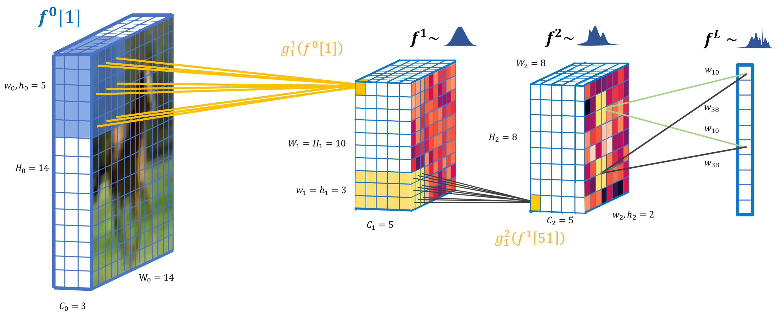
We assume an image representation of width and height pixels at layer . We collect channels into a 3D tensor , where the channels are along the depth axis. The input image is the sized representation of the original image with C color channels. For instance MNIST images are of size pixels and have a single grayscale channel.
We decompose the 3D tensor into patches containing all depth channel. and are the height and width of the image patch at layer . We index patches by . and denotes the height and width of the output of layer . We compose a sequence of layers that map the input image to the label :
| (10) |
Layers with are random variables with probability densities .
We construct the layers by applying convolutions of patch response functions over the input one patch at a time producing the next layer representation:
| (11) |
Each individual patch response is a pixel stack. By repeating the patch responses over the patches we form a new representation (See Figure 1).
We model the patch responses at each of the first layers as independent GPs with shared prior
| (12) |
for . The kernel measures the similarity of two image patches. The standard property of Gaussian processes implies that the functions output similar responses for similar patches.


For example, on MNIST where images have size using patches of size , a stride of 1 and patch response functions, we obtain a representation of size after the first layer (height and width ). This is passed on to the next layer which produces an output of size .
We follow the sparse GP approach of Hensman et al. (2015a) and augment each patch response function by a set of inducing patches in the patch space with corresponding responses . Each layer contains inducing patches which are shared among the patch response functions within that layer. Each patch response function has separate inducing responses which associate outputs to each inducing patch. We collect these into a matrix .
The conditional patch responses are
| (13) | ||||
where the covariance between the input and the inducing variables are
a matrix of size that measures the similarity of all patches against all filters . We set the base kernel to be the RBF kernel. For each of the patch response functions we obtain one output image channel.
In contrast to neural networks, the Gaussian process convolutions induce probabilistic layer representations. The first layer is a Gaussian directly from (13), while the following layers follow non-Gaussian distributions since we map all realisations of the random input into Gaussian outputs .
3.2 Final classification layer
As the last layer of our model we aggregate the output of the convolutional layers using a GP with a weighted convolutional kernel as presented by Van der Wilk et al. (2017). We set a GP prior on the last layer patch response function
| (14) |
with weights for each patch response. We get an additive GP
where the kernel is the weighted average patch similarity of the final tensor representation . . The matrix collects all patch similarities . The last layer has one response GP per output class .
As with the convolutional layers the inducing points live in the patch space of instead of in the image space. The inter-domain kernel is
| (15) | ||||
| (16) |
The kernel collects all patch similarities of a single image compared against inducing points . The covariance between inducing points is simply . We have now defined all kernels necessary to evaluate and optimize the variational bound (9).
3.3 Doubly stochastic variational inference
| Inducing | Test accuracy | ||||
| Gaussian process models | Layers | points | MNIST | CIFAR-10 | Reference |
| RBF AutoGP | Krauth et al. (2017) | ||||
| Multi-channel conv GP | Van der Wilk et al. (2017) | ||||
| DeepCGP | 98.38 | 58.65 | current work | ||
| DeepCGP | 99.24 | 73.85 | ” | ||
| DeepCGP | 99.44 | 75.89 | ” | ||
| Neural network models | Layers | # params | |||
| Deep kernel learning | 5 | 2.3M .. 4.6M | Wilson et al. (2016a) | ||
| DenseNet | 250 | 15.3M | N/A | Huang et al. (2017) | |
The deep convolutional Gaussian process is an instance of a deep Gaussian process with the convolutional kernels and patch filter inducing points. We follow the doubly stochastic variational inference approach of Salimbeni and Deisenroth (2017) for model learning. The key idea of doubly stochastic inference is to draw samples from the Gaussian
| (17) |
through the deep system for a single input image .
The inducing points of each layer are independent. We assume a factorised likelihood
| (18) |
and a true joint density
| (19) | ||||
| (20) |
The evidence framework MacKay (1992) considers optimizing the evidence,
| (21) |
Following the variational approach we assume a variational joint model
| (22) | ||||
| (23) |
The distribution of the layer predictions depends on current layer inducing points and representation at the previous layer. By marginalising the variational approximation we arrive at the factorized variational posterior of the last layer for individual data point ,
| (24) |
where we integrate all paths through the layers defined by the filters , and the parameters . Finally, the doubly stochastic evidence lower bound (ELBO) is
| (25) | ||||
The variational expected likelihood is computed using a Monte Carlo approximation yielding the first source of stochasticity. The whole lower bound is optimized using stochastic gradient descent yielding the second source of stochasticity.
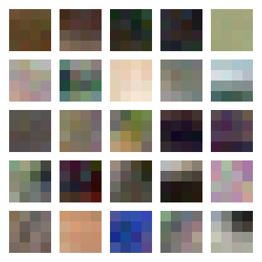
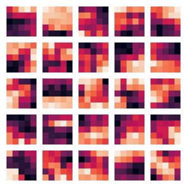
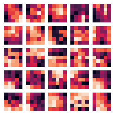
The Figure 2 visualises representations of CIFAR-10 images over the deep convolutional GP model. Figure 3 visualises the patch and filter spaces of the three layers, indicating high overlap. Finally, Figure 4 shows example filters learned on the CIFAR-10 dataset, which extract image features.
Optimization
All parameters , , , the base kernel RBF lengthscales and variances and the patch weights for the last layer are learned using stochastic gradient Adam optimizer (Kingma and Ba, 2014) by maximizing the likelihood lower bound. We use one shared base kernel for each layer.
4 Experiments
We compare our approach on the standard image classification benchmarks of MNIST and CIFAR-10 (Krizhevsky and Hinton, 2009), which have standard training and test folds to facilitate direct performance comparisons. MNIST contains 60,000 training examples of sized grayscale images of 10 hand-drawn digits, with a separate 10,000 validation set. CIFAR-10 contains 50,000 training examples of RGB colour images of size from 10 classes, with 5,000 images per class. The images represents objects such as airplanes, cats or horses. There is a separate validation set of 10,000 images. We preprocess the images for zero mean and unit variance along the color channel.
We compare our model primarily against the original shallow convolutional Gaussian process (Van der Wilk et al., 2017), which is currently the only convolutional Gaussian process based image classifier. We also consider the performance of the hybrid neural network GP approach of Wilson et al. (2016a). For completeness we report the performance of a state-of-the-art CNN method DenseNet (Huang et al., 2017).
Implementation.
Our TensorFlow (Abadi et al., 2016) implementation is compatible with the GPflow framework
(Matthews et al., 2017) and freely available online 111https://github.com/kekeblom/DeepCGP. We leverage GPU accelerated computation, 64bit floating point precision, and employ a minibatch size of 32.
We start the Adam learning rate at and multiply it by every 100,000 optimization steps until the learning rate reaches 1e-5. We use inducing points at each layer. We set a stride of for the first layer and for all other layers. The convolutional filter size is 5x5 on all layers except for the first layer on CIFAR-10 where it is 4x4. This is to make use of all the image pixels using a stride of 2.
Parameter initialization.
Inducing points are initialized by running -means with clusters on image patches from the training set. The variational means are initialised to zero. are initialised to a tiny variance kernel prior following Salimbeni and Deisenroth (2017), except for the last layer where we use . For models deeper than two layers, we employ iterative optimisation where the first layers and layer are initialised to the learned values of an model, while the one additional layer added before the classification layer is initialised to default values.
4.1 MNIST and CIFAR-10 results
Table 1 shows the classification accuracy on MNIST and CIFAR-10. Adding a convolutional layer to the weighted convolutional kernel GP improves performance on CIFAR-10 from 58.65% to 73.85%. Adding another convolutional layer further improves the accuracy to 75.9%. On MNIST the performance increases from error to error with the three-layer deep convolutional GP.
The deep kernel learning method uses a fully connected five-layer DNN instead of a CNN, and performs similarly to our model, but with much more parameters.
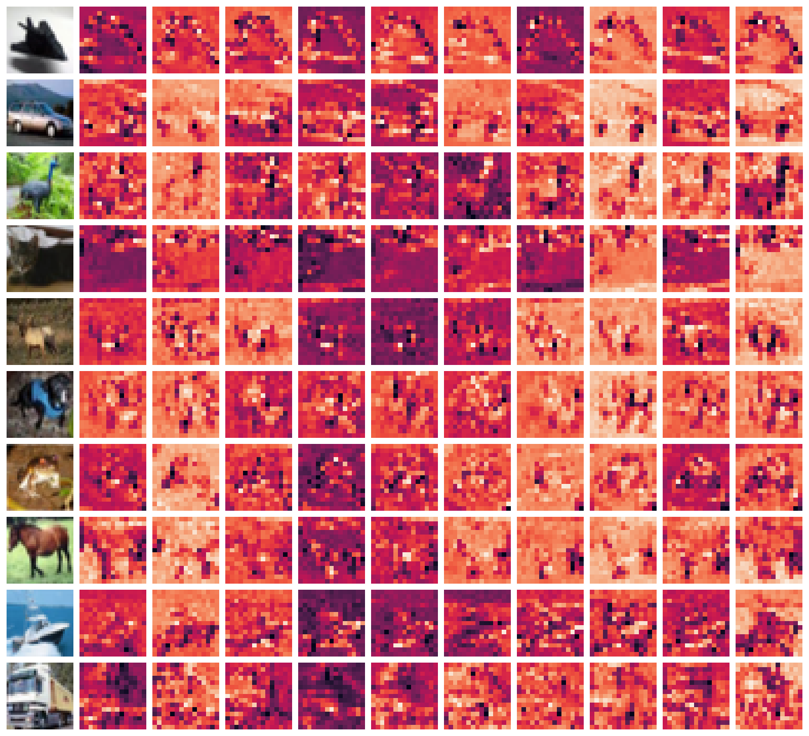
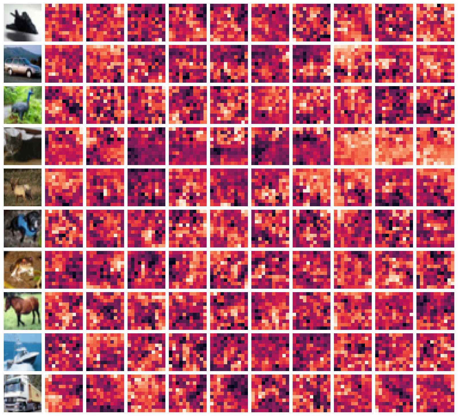
Figure 5 shows a single sample for 10 image class examples (rows) over the 10 patch response channels (columns) for the first layer (panel a) and second layer (panel b). The first layer indicates various edge detectors, while the second layer samples show the complexity of pattern extraction. The row object classes map to different kinds of representations, as expected.
Figure 2 shows UMAP embedding McInnes and Healy (2018) visualisations of the image space of CIFAR-10 along with the structure of the layer representations for three layers. The original images do not naturally cluster into the 10 classes (a). The DCGP model projects the images to circle shape with some class coherence in the intermediate layers, while the last layer shows the classification boundaries. An accompanying Figure 4 shows the learned inducing filters and layer patches on CIFAR-10. Some regions of the patch space are not covered by filters, indicating uninformative representations.
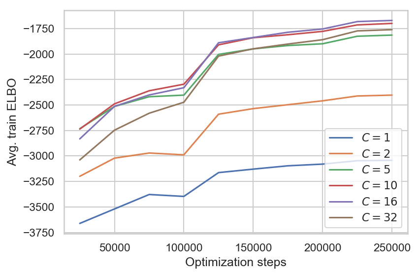
Figure 6 shows the effect of different channel numbers on a two layer model. The ELBO increases up to response channels, while starts to decrease with channels. A model with approximately channels indicates best performance.
5 Conclusions
We presented a new type of deep Gaussian process with convolutional structure. The convolutional GP layers gradually linearize the data using multiple filters with nonlinear kernel functions. Our model greatly improves test results on the compared classification benchmarks compared to other GP-based approaches, and approaches the performance of hybrid neural-GP methods. The performance of our model seems to improve as more layers are added.
We did not experiment with using a stride of 1 at the first layer. Neither did we try models with 4 or more layers. The added complexity comes with an increased computational cost and we were thus limited from experimenting with these improvements. We believe that both of these enhancements would increase performance.
Deep Gaussian process models lead to degenerate covariances, where each layer in the composition reduces the rank or degrees of freedom of the system (Duvenaud et al., 2014). In practise the rank reduces via successive layers mapping inputs to identical values, effectively merging inputs and resulting in rank-reducing covariance matrix with repeated rows and columns. To counter this pathology Salimbeni and Deisenroth (2017) proposed rank-preserving deep model by pseudo-monotonic layer mappings with GP priors with identity means . In contrast we employ zero-mean patch response functions. Remarkably we do not experience rank degeneracy, possibly due to the multiple channel mappings and the convolution structure.
There are several avenues for improved efficiency and modelling capacity. The Stochastic Gradient Hamiltonian Monte Carlo approach (Ma et al., 2015) has proven efficient in deep GPs (Havasi et al., 2018) and in GANs (Saatci and Wilson, 2017). Another avenue for improvement lies in kernel interpolation techniques (Wilson and Nickisch, 2015; Evans and Nair, 2018) which would make inference and prediction faster. We leave these directions for future work.
Acknowledgements
We thank Michael Riis Andersen for his invaluable comments and helpful suggestions.
References
- Abadi et al. (2016) Martín Abadi, Paul Barham, Jianmin Chen, Zhifeng Chen, Andy Davis, Jeffrey Dean, Matthieu Devin, Sanjay Ghemawat, Geoffrey Irving, Michael Isard, et al. Tensorflow: a system for large-scale machine learning. In OSDI, volume 16, pages 265–283, 2016.
- Blei et al. (2017) David M Blei, Alp Kucukelbir, and Jon D McAuliffe. Variational inference: A review for statisticians. Journal of the American Statistical Association, 112(518):859–877, 2017.
- Blundell et al. (2015) Charles Blundell, Julien Cornebise, Koray Kavukcuoglu, and Daan Wierstra. Weight uncertainty in neural networks. In International Conference on International Conference on Machine Learning, pages 1613–1622, 2015.
- Damianou and Lawrence (2013) Andreas Damianou and Neil Lawrence. Deep gaussian processes. In AISTATS, pages 207–215, 2013.
- Duvenaud et al. (2014) David Duvenaud, Oren Rippel, Ryan Adams, and Zoubin Ghahramani. Avoiding pathologies in very deep networks. In AISTATS, pages 202–210, 2014.
- Duvenaud et al. (2011) David K Duvenaud, Hannes Nickisch, and Carl E Rasmussen. Additive gaussian processes. In Advances in neural information processing systems, pages 226–234, 2011.
- Evans and Nair (2018) Trefor W Evans and Prasanth B Nair. Scalable gaussian processes with grid-structured eigenfunctions (GP-GRIEF). In International Conference on Machine Learning, 2018.
- Gal and Ghahramani (2016) Yarin Gal and Zoubin Ghahramani. Dropout as a bayesian approximation: Representing model uncertainty in deep learning. In International Conference on Machine Learning, pages 1050–1059, 2016.
- Garriga-Alonso et al. (2018) Adrià Garriga-Alonso, Laurence Aitchison, and Carl Edward Rasmussen. Deep convolutional networks as shallow gaussian processes. arXiv preprint arXiv:1808.05587, 2018.
- Goodfellow et al. (2016) Ian Goodfellow, Yoshua Bengio, Aaron Courville, and Yoshua Bengio. Deep learning, volume 1. MIT press Cambridge, 2016.
- Havasi et al. (2018) Marton Havasi, José Miguel Hernández Lobato, and Juan José Murillo Fuentes. Inference in deep gaussian processes using stochastic gradient hamiltonian monte carlo. arXiv preprint arXiv:1806.05490, 2018.
- Hensman et al. (2015a) James Hensman, Alexander G de G Matthews, and Zoubin Ghahramani. Scalable variational gaussian process classification. In AISTATS, pages 351–360, 2015a.
- Hensman et al. (2015b) James Hensman, Alexander G de G Matthews, and Zoubin Ghahramani. Scalable variational gaussian process classification. In AISTATS, 2015b.
- Huang et al. (2017) Gao Huang, Zhuang Liu, Laurens Van Der Maaten, and Kilian Q Weinberger. Densely connected convolutional networks. In CVPR, volume 1, page 3, 2017.
- Kingma and Ba (2014) Diederik P Kingma and Jimmy Lei Ba. Adam: Amethod for stochastic optimization. In Proc. 3rd Int. Conf. Learn. Representations, 2014.
- Krauth et al. (2017) Karl Krauth, Edwin V Bonilla, Kurt Cutajar, and Maurizio Filippone. Autogp: Exploring the capabilities and limitations of Gaussian process models. In Uncertainty in Artificial Intelligence, Sydney, Australia, 08 2017. URL http://www.eurecom.fr/publication/5038.
- Krizhevsky and Hinton (2009) Alex Krizhevsky and Geoffrey Hinton. Learning multiple layers of features from tiny images. Technical report, Citeseer, 2009.
- Kumar et al. (2018) Vinayak Kumar, Vaibhav Singh, PK Srijith, and Andreas Damianou. Deep gaussian processes with convolutional kernels. arXiv preprint arXiv:1806.01655, 2018.
- Lee et al. (2017) Jaehoon Lee, Yasaman Bahri, Roman Novak, Samuel S Schoenholz, Jeffrey Pennington, and Jascha Sohl-Dickstein. Deep neural networks as gaussian processes. arXiv preprint arXiv:1711.00165, 2017.
- Ma et al. (2015) Yi-An Ma, Tianqi Chen, and Emily Fox. A complete recipe for stochastic gradient mcmc. In Advances in Neural Information Processing Systems, pages 2917–2925, 2015.
- MacKay (1992) David JC MacKay. A practical bayesian framework for backpropagation networks. Neural computation, 4:448–472, 1992.
- Mallat (2016) Stéphane Mallat. Understanding deep convolutional networks. Phil. Trans. R. Soc. A, 374(2065):20150203, 2016.
- Matthews et al. (2017) Alexander G. de G. Matthews, Mark van der Wilk, Tom Nickson, Keisuke. Fujii, Alexis Boukouvalas, Pablo León-Villagrá, Zoubin Ghahramani, and James Hensman. GPflow: A Gaussian process library using TensorFlow. Journal of Machine Learning Research, 18(40):1–6, apr 2017. URL http://jmlr.org/papers/v18/16-537.html.
- McInnes and Healy (2018) L. McInnes and J. Healy. UMAP: Uniform Manifold Approximation and Projection for Dimension Reduction. ArXiv e-prints, February 2018.
- Rasmussen (2004) Carl Edward Rasmussen. Gaussian processes in machine learning. In Advanced lectures on machine learning, pages 63–71. Springer, 2004.
- Rasmussen and Williams (2006) Carl Edward Rasmussen and Christopher KI Williams. Gaussian process for machine learning. MIT press, 2006.
- Remes et al. (2017) Sami Remes, Markus Heinonen, and Samuel Kaski. Non-stationary spectral kernels. In Advances in Neural Information Processing Systems, pages 4642–4651, 2017.
- Saatci and Wilson (2017) Yunus Saatci and Andrew G Wilson. Bayesian gan. In Advances in neural information processing systems, pages 3622–3631, 2017.
- Salimbeni and Deisenroth (2017) Hugh Salimbeni and Marc Deisenroth. Doubly stochastic variational inference for deep gaussian processes. In Advances in Neural Information Processing Systems, pages 4588–4599, 2017.
- Snelson and Ghahramani (2006) Edward Snelson and Zoubin Ghahramani. Sparse gaussian processes using pseudo-inputs. In Advances in neural information processing systems, pages 1257–1264, 2006.
- Sun et al. (2018) S. Sun, G. Zhang, C. Wang, W. Zeng, J. Li, and R. Grosse. Differentiable compositional kernel learning for gaussian processes. In ICML, 2018.
- Van der Wilk et al. (2017) Mark Van der Wilk, Carl Edward Rasmussen, and James Hensman. Convolutional gaussian processes. In Advances in Neural Information Processing Systems, pages 2849–2858, 2017.
- Williams (1997) Christopher KI Williams. Computing with infinite networks. In Advances in Neural Information Processing Systems, pages 295–301, 1997.
- Wilson et al. (2013) A. Wilson, E. Gilboa, A. Nehorai, and J. Cunningham. Fast multidimensional pattern extrapolation with gaussian processes. AISTATS, 2013.
- Wilson and Nickisch (2015) Andrew Wilson and Hannes Nickisch. Kernel interpolation for scalable structured gaussian processes (kiss-gp). In International Conference on Machine Learning, pages 1775–1784, 2015.
- Wilson et al. (2016a) Andrew G Wilson, Zhiting Hu, Ruslan R Salakhutdinov, and Eric P Xing. Stochastic variational deep kernel learning. In Advances in Neural Information Processing Systems, pages 2586–2594, 2016a.
- Wilson et al. (2016b) Andrew Gordon Wilson, Zhiting Hu, Ruslan Salakhutdinov, and Eric P Xing. Deep kernel learning. In AISTATS, pages 370–378, 2016b.