Planet Occurrence Rate Density Models Including Stellar Effective Temperature
Abstract
We present planet occurrence rate density models fit to Kepler data as a function of semi-major axis, planetary radius, and stellar effective temperature. We find that occurrence rates for M type stars with lower effective temperature do not follow the same trend as F, G, and K type stars when including a polynomial function of effective temperature in an occurrence rate density model and a better model fit includes a break in effective temperature. Our model fit for M type stars consists of power laws on semi-major axis and planetary radius. Our model fit for F, G, and K type stars consists of power laws on semi-major axis and planetary radius broken at 2.771 and a quadratic function of stellar effective temperature. Our models show agreement with published occurrence rate studies and are the first to explicitly include stellar effective temperature as a variable. By introducing stellar effective temperature into our occurrence rate density models, we enable more accurate occurrence rate predictions for individual stars in mission simulation and science yield calculations for future and proposed exoplanet finding missions.
1 Introduction
Exoplanet-finding surveys have shown that planets are common (Winn & Fabrycky, 2015; Winn, 2018). From these surveys the occurrence rate of planets may be inferred by applying a completeness or detection efficiency correction (correcting for observational or algorithmic biases which led to missed detections of real planets, e.g. Christiansen et al. (2015)) to the number of planets discovered with properties binned in a specified range (typically mass and orbital period for radial velocity, as in Cumming et al. (2008), or planet radius and period for transit surveys, as in Howard et al. (2012)). Accurately determining occurrence rates requires a large sample of target stars, planet detections, and knowledge of specific instrument effects (Tabachnik & Tremaine, 2002; Youdin, 2011; Batalha, 2014). A model fit to occurrence rate densities can then be used to interpolate or extrapolate occurrence rates for a desired range of parameters (Catanzarite & Shao, 2011; Traub, 2011; Biller et al., 2013; Kopparapu et al., 2013; Petigura et al., 2013a; Burke et al., 2015). For direct imaging surveys, such as the proposed Wide-Field Infrared Survey Telescope’s (WFIRST) Coronagraph Instrument (Spergel et al., 2015), these occurrence rate densities can be used to generate planet populations for completeness studies (Brown, 2005; Brown & Soummer, 2010; Garrett & Savransky, 2016), exoplanet yield maximization (Stark et al., 2014), or full mission simulations (Savransky & Garrett, 2015).
The earliest models for planet occurrence rate densities were based on radial velocity surveys. Tabachnik & Tremaine (2002) fit a joint power-law model to the occurrence rate densities of the 72 planets detected up to that point via the radial velocity method with and days, where is the mass of the planet and is the orbital period. Cumming et al. (2008) established a benchmark model for occurrence rates by fitting a joint power law to occurrence rate densities for and days from a radial velocity survey consisting of 600 F, G, K, and M type stars monitored over eight years. Howard et al. (2010a) extended the results of Cumming et al. (2008) to lower masses by fitting a joint power law to the occurrence rate densities of planets for 166 G and K type stars with and days. Bryan et al. (2016) fit a power law on mass, , and semi-major axis, , to data collected at the Keck Observatory as a part of the California Planet Study (Howard et al., 2010b).
The Kepler mission (Batalha, 2014; Borucki, 2017) has yielded thousands of planet discoveries via the transit method and enabled investigation of occurrence rates of Earth-like planets. Many studies have fit occurrence rate density models to various period and radius ranges, stellar types, and Kepler data releases. Youdin (2011), Burke et al. (2015), and Mulders et al. (2018) fit occurrence rate densities on period and planetary radius, , jointly. A number of studies fit occurrence rate densities only dependent on period (Howard et al., 2012; Catanzarite & Shao, 2011; Traub, 2011; Dong & Zhu, 2013; Petigura et al., 2013b; Silburt et al., 2015) or planetary radius (Howard et al., 2012; Catanzarite & Shao, 2011; Morton & Swift, 2014). Primarily, these models have been power laws, however, Berta et al. (2013) fit a joint model which has power law and sigmoid terms and Morton & Swift (2014) used a weighted kernel density estimation (wKDE) approach. A summary of these models based on period and planetary radius along with the fit type, period and planetary radius ranges, stellar spectral type, and Kepler release data is given in Table LABEL:tab:literature. Models based on Kepler data are not restricted to period and planetary radius. Recently, Pascucci et al. (2018) fit broken power laws to occurrence rate density dependent on planet-to-star mass ratio for F, G, K, and M type stars using Kepler Q1-Q17 data.
Direct imaging surveys are sensitive to large planets at large separations from their host stars (Bowler & Nielsen, 2018) and complement other exoplanet detection techniques. Although fewer detections have been made via direct imaging, it has been shown that occurrence rate models from radial velocity or transit surveys cannot be extrapolated to the region probed by direct imaging and constraints on the occurrence rates at wide separations have been determined (Lafreniere et al., 2007; Nielsen et al., 2008; Nielsen & Close, 2010; Biller et al., 2013; Wahhaj et al., 2013; Brandt et al., 2014; Vigan et al., 2017). These constraints have been used to synthesize models from microlensing, radial velocity, and direct imaging surveys (Clanton & Gaudi, 2014, 2016).
All of the occurrence rate models mentioned are only dependent on planet and orbital properties. However, occurrence rates are dependent on stellar properties like metallicity and effective temperature (Winn, 2018; Mulders, 2018). Marcy et al. (2005) showed that planet occurrence rises with stellar metalicity. Radial velocity surveys have shown that giant planet occurrence rates are associated with higher stellar metallicity (Gonzalez, 1997; Santos et al., 2004; Valenti & Fischer, 2005; Mayor et al., 2011; Reffert et al., 2015) while smaller planets are not (Sousa et al., 2008; Buchhave et al., 2012; Beaugé & Nesvornỳ, 2012). Schlaufman (2018) found this association with high metallicity to be weaker. For periods shorter than 10 days, small planets are associated with higher metallicities (Mulders et al., 2016; Petigura et al., 2018; Wilson et al., 2018). Zhu et al. (2016) found that the planet-metallicity correlation for small planets could be the same as that for giant planets. Using Kepler data, Petigura et al. (2018) fit an occurrence rate density model to period and stellar metallicity.
Kepler data has been used to investigate the effect of stellar effective temperature, , on planet occurrence rates. Traub (2011) found that for periods less than 42 days, the occurrence rates for terrestrial planets are roughly the same, ice giants vary by a factor of two, and gas giants rapidly drop with for F, G, and K type stars. Howard et al. (2012) and Mulders et al. (2015a, b) found that smaller planets occur more frequently around stars with lower . Dressing & Charbonneau (2013, 2015) supported this finding by investigating the occurrence rates of small planets around M dwarfs. Fressin et al. (2013) investigated the effect of stellar mass, which is related to , on the occurrence rate of planets in various radius bins, and found that giant planet (6–22) occurrence rates increase with for M, K, and G type stars and then decrease with for F type stars. The same work found no dependence on for large Neptunes (4–6) and small Neptunes (2–4).
We present planet occurrence rate density models fit to previous occurrence rate calculations from the Kepler literature and data from NASA’s Exoplanet Program Analysis Group (ExoPAG) Science Analysis Group 13111https://exoplanets.nasa.gov/exep/exopag/sag/ (hereafter SAG13) which include the planet parameters of semi-major axis, , and planetary radius, , while also incorporating (Section 2). We discuss our data selection (Section 3), model fitting process (Section 4), and results (Section 5). Finally, we compare our models to data from the literature (Section 6).
2 Planet Occurrence Rate Models with Stellar Effective Temperature
Mulders et al. (2015a) showed that by stretching the semi-major axis and multiplying the overall occurrence rate by a fractional value dependent on , the occurrence rates of 1–4 planets for M, K, and G type stars collapse onto the occurrence rates of F stars (see Mulders et al. (2015a) Figure 4). The scaling relationship between semi-major axis and stellar mass for the cutoff of occurrence rates near a period of 10 days for different spectral type stars is given by (Mulders et al., 2015a; Lee & Chiang, 2017). Since stellar mass can be represented as a function of , we represent both the semi-major axis stretching and overall occurrence rate scaling as a single function of . We wish to reference our model to solar and Earth values, so we normalize by , , and . We define
| (1) |
to work with numerical values on a similar scale. We define the dependent portion of our occurrence rate density model as a power series with as many terms as necessary in
| (2) |
Our simple occurrence rate density model is given as
| (3) |
where , , , as well as the values and number of terms in are determined by fitting the model to data. In addition to this simple model, we investigate a break radius model similar to Burke et al. (2015)
| (4) |
where the break radius, , as well as two sets of constants for and are determined via fitting to data.
3 Data Selection
We seek occurrence rate data binned on a wide range of planet properties (orbital period and planetary radius) and . The SAG13 effort collected tables of occurrence rates from Kepler data and defined a standard grid of planetary radius, orbital period, and stellar type. The occurrence rates came from data and models from peer-reviewed publications (Petigura et al., 2013a; Foreman-Mackey et al., 2014; Burke et al., 2015; Dressing & Charbonneau, 2015; Mulders et al., 2015b, a, 2016; Traub, 2016; Fulton et al., 2017) and unpublished tables generated by Natalie Batalha, Ruslan Belikov, Joseph Catanzarite, Will Farr, and Ravi Kopparapu using the Q1-Q16 or Q1-Q17 planet candidates, DR24 star properties catalog, and Kepler completeness curves released in the fall of 2015.
The SAG13 standard planetary radius-period grid consists of uniformly spaced bins in log radius and period, where the th planet radius bin is given by
| (5) |
(bin edges ) and the th orbital period bin given by
| (6) |
(bin edges days). Unless otherwise indicated, the stellar types are grouped as
| (7) |
For G type stars, the SAG13 group found the sample geometric mean and variance from all of the submissions in each bin of the period-radius grid. They then performed three least-squares fits of joint power laws broken by radius of the form
| (8) |
The mean occurrence rate values were used to generate a “baseline” fit, the mean minus the standard deviation generated a “pessimistic” fit, and the mean plus the standard deviation generated an “optimistic” fit. The break between the two pieces of the power law was chosen to be 3.4 to align with Burke et al. (2015) and for similar reasons. The parameter values found by least-squares are shown in Table 1 where the set of , , and correspond to the parameters for and the other parameters correspond to . It should be noted that the SAG13 power laws may not hold if extrapolated to regions where Kepler has poor reliability and completeness, including long period and/or small planets. In particular, a power law in period with will violate the Hill stability criterion for a large enough period, so any extrapolation must either truncate the power law for some large , or set .
| Pessimistic | Baseline | Optimistic | |
|---|---|---|---|
| 0.138 | 0.38 | 1.06 | |
| 0.72 | 0.73 | 0.78 | |
| 0.204 | 0.26 | 0.32 | |
| 0.51 | 0.59 | 0.67 | |
| 0.277 | -0.19 | -0.68 | |
| -1.56 | -1.18 | -0.82 |
The likelihood function we use for our model fits requires knowledge of the occurrence rate uncertainty. Many of the data tables from SAG13 do not include uncertainty information on the occurrence rates, so we use the subset of SAG13 data tables that includes occurrence rate 1 uncertainty information. We select the SAG13 data from the folders “Natalie9p1” (hereafter “Batalha”, asymmetric uncertainties for M, K, and G type stars), “Mulders” (symmetric uncertainties for M, K, G, and F type stars), and “Burke” (asymmetric uncertainties for M and GK type stars). “Batalha,” contributed by Natalie Batalha, contains unpublished occurrence rate tables using the Q1-Q16 Kepler planet catalog (Mullally et al., 2015), DR24 star properties (Huber et al., 2014), and the completeness calculation of Christiansen et al. (2015) with the analytic approximation to the window function given by Burke et al. (2015). “Mulders,” contributed by Gijs Mulders, also uses the Q1-Q16 Kepler planet catalog (Mullally et al., 2015), DR24 star properties (Huber et al., 2014), and the completeness calculation of Christiansen et al. (2015) as described in Mulders et al. (2015b) and Mulders et al. (2015a). “Burke,” contributed by Chris Burke, follows Burke et al. (2015) in using the Q1-Q16 Kepler planet catalog (Mullally et al., 2015) and pipeline completeness model from Christiansen et al. (2015). We do not include published data from Fressin et al. (2013) or Christiansen et al. (2015) because the range in those studies combine F, G, and K type stars. We use the data from Dressing & Charbonneau (2015) for M type stars as independent test data and do not include it in the data set for model fitting.
We note that we selected community-sourced data from SAG13 using Kepler DR24 results and do not use the most recent and comprehensive Kepler planet catalog (Thompson et al., 2018), revised stellar properties (Mathur et al., 2017; Berger et al., 2018), Kepler pipeline (Jenkins, 2017), detection efficiencies (Christiansen, 2017), or Robovetter vetting process (Coughlin, 2017) from DR25. Kopparapu et al. (2018) used the planet list from Thompson et al. (2018), stellar properties from Mathur et al. (2017), and completeness calculations with KeplerPORT (Burke & Catanzarite, 2017) to compare DR25 based occurrence rates with SAG13 occurrence rates. The SAG13 occurrence rates (Table 3 from Kopparapu et al. (2018)) and DR25 based occurrence rates (Table 4 from Kopparapu et al. (2018)) are consistent and the DR25 occurrence rates are within the uncertainties of the baseline SAG13 occurrence rates. Because the data we selected comes from SAG13, the comparison done by Kopparapu et al. (2018) shows that our model fits will be within the uncertainty of Kepler DR25 based occurrence rates.
We assume that the uncertainties on occurrence rates are symmetric and Gaussian so that we may use a Gaussian likelihood function. When the uncertainties on occurrence rates from the data are asymmetric , we use data where the uncertainties are within 20% of each other (Chen & Kipping, 2016). We take the average of the remaining asymmetric uncertainties (Weiss & Marcy, 2014; Wolfgang et al., 2016) to give the standard deviation of the occurrence rates. We find no significant difference in our model fits when using data where the asymmetric uncertainties are within 10% or 20%, however, using the 20% limit includes more data. We also remove cases where the lower bound on the occurrence rate uncertainty would result in an occurrence rate of zero. These cuts remove 13% of the data but result in symmetric uncertainties which may be used with a Gaussian likelihood function.
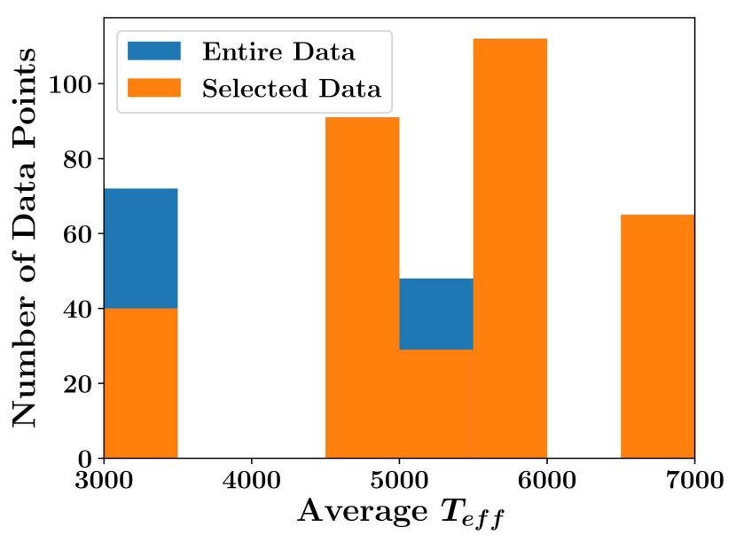
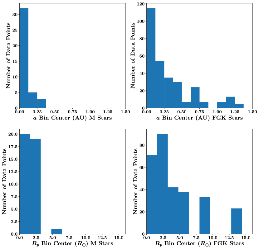
For each of the occurrence rate data tables grouped by stellar spectral type in “Batalha,” “Mulders,” and “Burke,” we take the arithmetic average of the bin edges given in the meta-data, or take the arithmetic average of the SAG13 standard stellar spectral type bin edges when not given in the meta-data, and use these average values as inputs to our occurrence rate density models. Figure 1 shows the distribution of average for the entire data set and the selected data set. For each data set, we convert period bins to semi-major axis bins by finding the average stellar mass using the mass- relation from Pecaut & Mamajek (2013)222http://www.pas.rochester.edu/~emamajek/EEM_dwarf_UBVIJHK_colors_Teff.txt. Figure 2 shows the distributions of the selected semi-major axis and planet radius split between M type stars and F, G, and K type stars. Table 2 provides an overall summary of the entire data set and selected data. Since Kepler’s objective is to determine the frequency of Earth-sized planets in the habitable zone of sun-like stars (Batalha, 2014; Borucki, 2017), it is unsurprising that our selected data is concentrated near sun-like stars with small, close-in planets.
| Source | (K) | Spectral Type | (AU) | Data Points | |
| Batalha | M | 10 (10) | |||
| K | 34 (34) | ||||
| G | 40 (40) | ||||
| Mulders | M | 27 (27) | |||
| K | 57 (57) | ||||
| G | 72 (72) | ||||
| F | 65 (65) | ||||
| Burke | M | 35 (3) | |||
| GK | 48 (29) | ||||
| Total | 388 (337) |
4 Fitting Planet Occurrence Rate Models
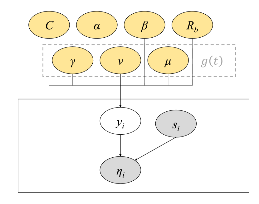
We use Bayesian parameter estimation with Markov Chain Monte Carlo (MCMC) sampling to evaluate the posterior distribution of our model parameters via the Python package emcee (Foreman-Mackey et al., 2013)333https://github.com/dfm/emcee. The hierarchical model for our occurrence rate density model is shown in Figure 3. To sample from the posterior distribution, we require a likelihood function and prior. We assume a Gaussian likelihood function where the log-likelihood is given by
| (9) |
where is the occurrence rate from the data, is the 1 error bar from the data, and
| (10) |
is the occurrence rate determined from our model for occurrence rate density integrated over the lower and upper bin edges from the data. Our priors for both the simple and break radius models are given by
| (11) |
where denotes a uniform distribution. Occurrence rates by definition are non-negative, so we sample to ensure this constraint. The power law indices for period and planetary radius from the literature tend to fall in the range of (-1,1), so we expand these limits to (-2,2) in our prior distributions. We set the limits of the prior to the full range of in our data set. We have no knowledge of the constants in , so the limits on their prior distributions are wide. The values of from our data are limited to (-0.6,0.3) and the (linear coefficient), (quadratic coefficient), and (cubic coefficient) terms have increasingly wide prior distribution limits.
We first perform a minimization for the model parameters to find initial values for the walkers in emcee (Foreman-Mackey et al., 2013). For each set of posterior samples, we run 500 walkers for each parameter. The walkers must be initialized with differing values (Goodman & Weare, 2010; Foreman-Mackey et al., 2013), so we initialized each walker in the neighborhood of the minimization result by taking the minimization result and adding times a random sample of a zero mean Gaussian with standard deviation of one. We discard a “burn-in” set of samples of 1000 steps and run 1000 additional steps to generate the final set of 500,000 samples for each parameter. The code generating this data, “burn-in” samples, and final posterior samples can be found in the github repository dgarrett622/Occurrence.
5 Results
To evaluate the goodness of fit for our models, we report values of , , and the Bayesian Information Criterion (BIC) (Schwarz et al., 1978),
| (12) |
evaluated at the median value of each parameter, where is the total number of data points and is the number of parameters in the model. The model with the lowest BIC is preferred and differences larger than 10 are very strong, six to 10 are strong, two to six are positive, and zero to two are not significant (Kass & Raftery, 1995). We note that BIC performs better as a selection metric when (Schwarz et al., 1978). When the number of model parameters is large, BIC has the potential to give a lower value due to over-fitting.
We first investigate the simple models with no break radius fit to all of the selected data. We find the model fit parameters for the simple model with no dependence on (SMAll), linear dependence on (SMtAll), quadratic dependence on (SMt2All), and cubic dependence on (SMt3All). We report the 16th, 50th, and 84th percentiles for each of the parameters from their marginalized distributions as well as , , and BIC goodness of fit values for the 50th percentile model parameter values in Table 3. It is clear from the reduction in and BIC from SMAll to SMtAll that including in the model results in a better fit. From Table 3, it appears that including more terms in also results in better fits to the data.
| SMAll | SMAll | SM2All | SM3All | |
| -407.6 | -150.1 | -147.2 | -138.9 | |
| 3795 | 3280 | 3274 | 3257 | |
| 832.7 | 323.5 | 323.4 | 312.9 |
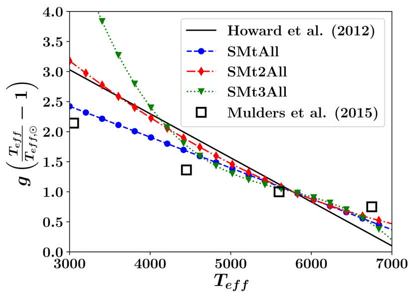
To determine which of the simple models is the best fit to available data, we compare our fit results to Howard et al. (2012) and Mulders et al. (2015a) in Figure 4. We normalize Equation 9 from Howard et al. (2012) (relating overall planet occurrence rates and ) such that it is 1 when . We take the values scaling the overall occurrence rates from Figure 4 of Mulders et al. (2015a) (for 1–4) and renormalize to G type stars to better represent our results normalized to solar . Howard et al. (2012) fit their Equation 9 to planet occurrence rate data for planets up to 0.25 AU and 2–4. The data for our model fits extend beyond their semi-major axis range and include a wider range for planetary radius, so it is unsurprising that our results give a different relation. However, as in Figure 8 of Howard et al. (2012) we find that overall planet occurrence rates decrease with increasing . SMtAll, SMt2All, and SMt3All diverge from each other for but converge for . This indicates that a break in may facilitate a better fit to the data.
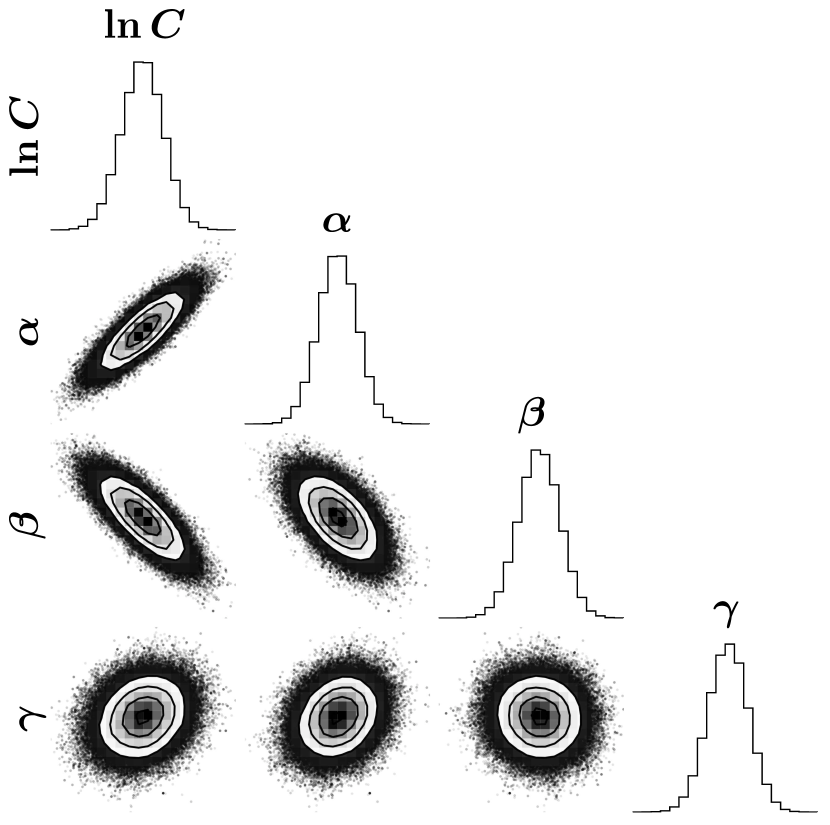
Although it has the best BIC value (Table 3), we do not consider the SMt3All model to be the preferred model because of the higher potential for over-fitting and large divergence from SMtAll and SMt2All (Figure 4). SMtAll and SMt2All are in the neighborhood of both Howard et al. (2012) and Mulders et al. (2015a) and have very nearly the same BIC. Because of this, we select the simpler SMtAll model as the preferred simple model fit to all of the selected data. We present a corner plot (Foreman-Mackey, 2016)444https://github.com/dfm/corner.py of the SMtAll model in Figure 5.
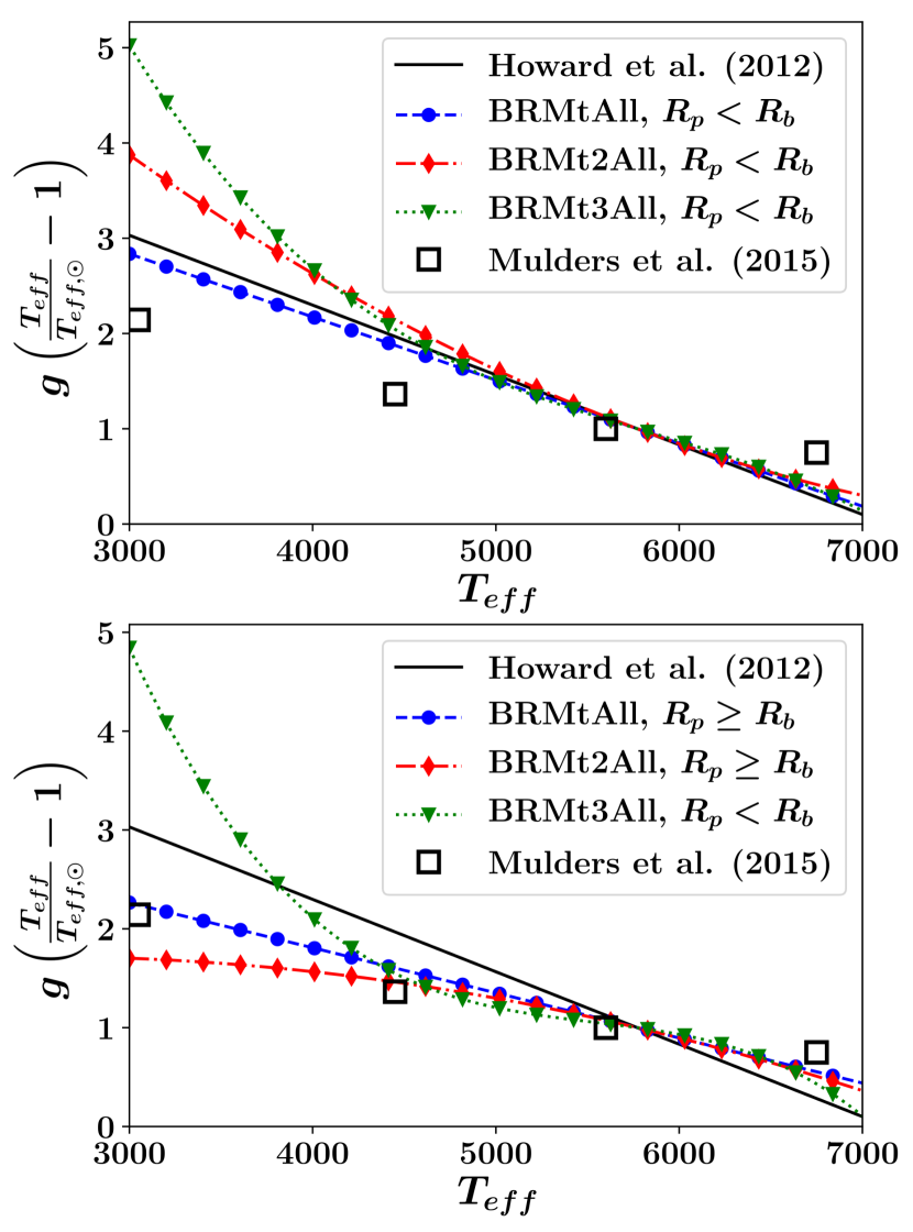
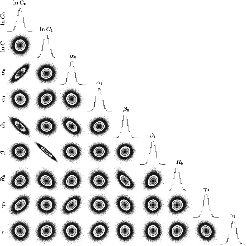
The break radius models fit to all of the selected data with no dependence on (BRMAll), linear dependence on (BRMtAll), quadratic dependence on (BRMt2All), and cubic dependence on (BRMt3All) follow similar trends to the simple models. We report the model parameter values at the 16th, 50th, and 84th percentile as well as the goodness of fit values evaluated at the model parameter 50th percentile values in Table 4. By any of the goodness of fit measures, the break radius model is a better fit than the equivalent version of the simple model. As with the simple models, the break radius models fit the data better when is included. We compare the break radius model fits to Howard et al. (2012) and Mulders et al. (2015a) in Figure 6. The top panel of Figure 6 shows our break radius models for and we see the same trend of decreasing occurrence rates with increasing as Howard et al. (2012). We also note that the BRMtAll model closely reproduces the result from Howard et al. (2012) for planets with . Howard et al. (2012) found that occurrence rates for planets larger than 4 have no correlation with . In the bottom panel of Figure 6 we find that occurrence rate decreases for increasing for planets larger than our break radius which does include some planets with , so we cannot make a direct comparison to the Howard et al. (2012) finding. As with the simple models, we also see the divergence of BRMtAll, BRMt2All, and BRMt3All near 4500 K. We find that the break radius for the BRMAll model is 3.027 which compares favorably to SAG13 (3.4) and Burke et al. (2015) (3.3) results. From Figure 6 and Table 4, the model which best matches the Mulders et al. (2015a) result and is preferred by BIC is BRMtAll. We present the corner plot of the BRMtAll model in Figure 7
| BRMAll | BRMAll | BRM2All | BRM3All | |
| -253.9 | 111.6 | 116.2 | 120.0 | |
| 3487 | 2756 | 2747 | 2739 | |
| 548.6 | -170.9 | -168.3 | -164.4 |
[ht]
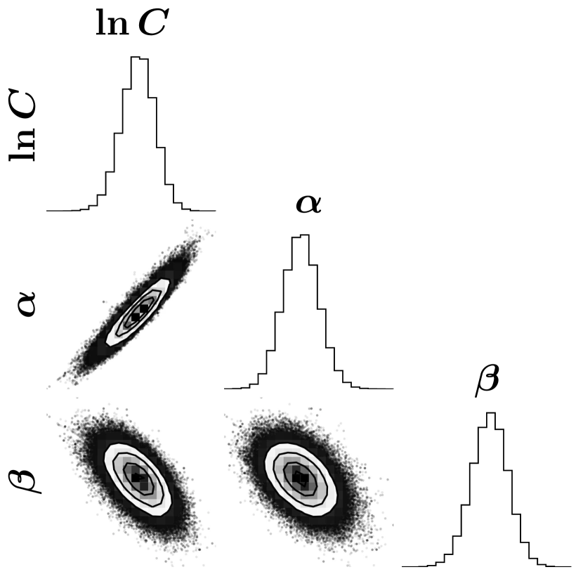
We split the data to investigate the divergence at lower seen in Figure 4 and Figure 6. We split the data for the M type stars from the data for the F, G, and K type stars. For the M type star sample, we are left with SAG13 data from “Batalha” (10 data points), “Mulders” (27 data points), and “Burke” (3 data points). Unfortunately, using the simple arithmetic mean of the bin edges from the meta-data results in the “Batalha” and “Mulders” data sets having the same average while the “Burke” data set has a different average but only three data points (as seen in Table 2). Because of this, we do not have sufficient data points to perform fits including for the M type star data set alone. We perform a simple model fit (SMM) to get the model parameter values at the 16th, 50th, and 84th percentile of their marginalized distributions and goodness of fit values as , , , , , and BIC = -118.4. We fit a break radius model to this data, however, there is no indication that a break radius model is better than the simple model. We note that the data for M type stars included in our model fitting contain very few planets larger than the break radii () determined by the model fits using the M, K, G, and F type star data (see Figure 2). This is likely the reason that a break radius model is not preferred over the simple model. A corner plot for the SMM model is given in Figure 8.
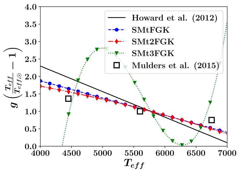
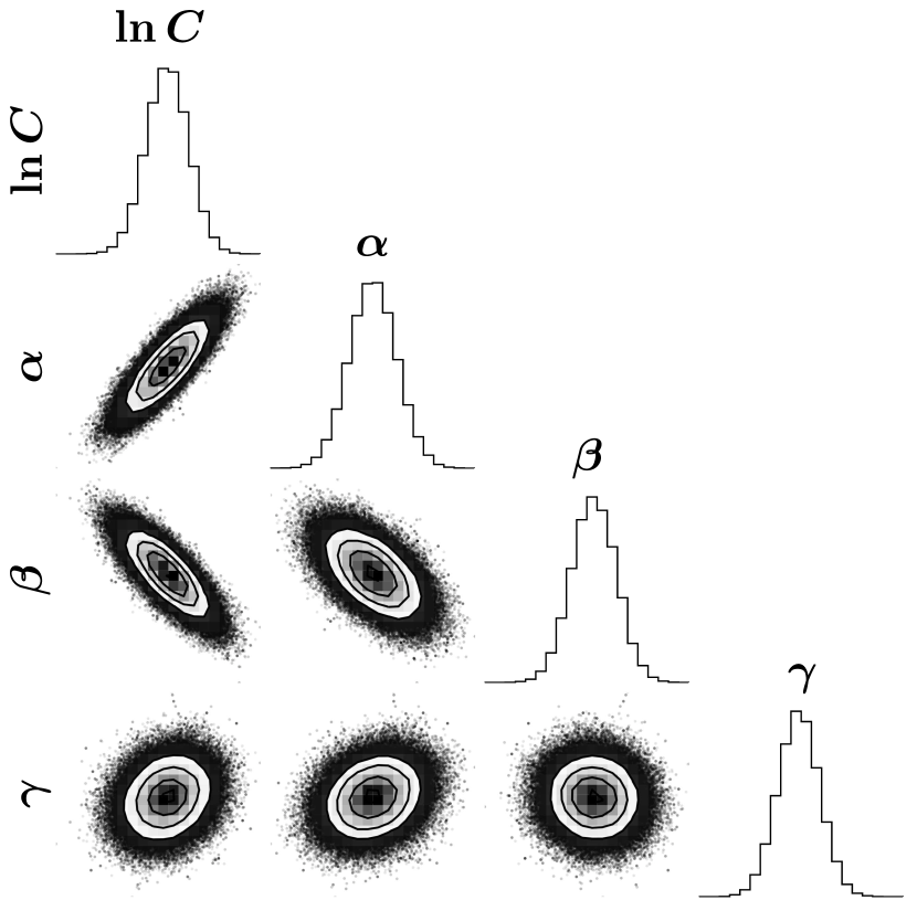
We present results for the simple models fit to the F, G, and K type star data with no break radius and no dependence on (SMFGK), linear dependence on (SMtFGK), quadratic dependence on (SMt2FGK), and cubic dependence on (SMt3FGK). We report the 16th, 50th, and 84th percentiles for each of the model parameters from their marginalized distributions as well as , , and BIC in Table 5. Similar trends are seen in the simple models for the F, G, and K type fits as for the simple models fit to the entire selected data set. We again plot the comparison to Howard et al. (2012) and Mulders et al. (2015a) in Figure 9 to determine which model is most accurate. The SMtFGK and SMt2FGK models show close agreement. Just as with the simple models fit to all of the selected data, the SMt3FGK model has a higher potential for over-fitting and shows large divergence from the other models and the data from Howard et al. (2012) and Mulders et al. (2015a) (Figure 9). Because of this, we do not select the SMt3FGK model as the preferred model even though it has the best BIC value (Table 5). Of the remaining models the one preferred by BIC is the SMtFGK model. We give a corner plot (Foreman-Mackey, 2016) of the SMtFGK model in Figure 10.
| SMFGK | SMFGK | SM2FGK | SM3FGK | |
| -395.2 | -164.6 | -163.9 | -96.50 | |
| 3560 | 3098 | 3097 | 2962 | |
| 807.5 | 352.0 | 356.3 | 227.2 |
[ht]
The break radius models fit to the F, G, and K type star data with no dependence on (BRMFGK), linear dependence on (BRMtFGK), quadratic dependence on (BRMt2FGK), and cubic dependence on (BRMt3FGK) follow similar trends to previous models. We report the model parameter values at the 16th, 50th, and 84th percentile values in Table 6. The break radius models are again better than the simple models fit to this data. We compare the break radius models for this data set to Howard et al. (2012) and Mulders et al. (2015a) in Figure 11. The top panel of Figure 11 shows our break radius models for and the bottom panel shows our break radius models for . The BRMtFGK and BRMt2FGK models closely reproduce the result from Howard et al. (2012) for . We find the break radius for the BRMFGK model is 3.060 which again compares favorably to SAG13 and Burke et al. (2015).
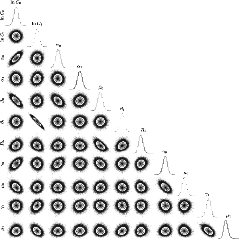
Even though the BIC value for the BRMt3FGK model is lower than the other models, we do not select it as the preferred model. As before, the BRMt3FGK model has a higher potential for over-fitting and exhibits large divergence from the other models and the data from Howard et al. (2012) and Mulders et al. (2015a). Visually, the BRMtFGK and BRMt2FGK give comparable results, however, the BRMt2FGK model is very strongly preferred by BIC. We give a corner plot (Foreman-Mackey, 2016) of the BRMt2FGK model in Figure 12.
| BRMFGK | BRMFGK | BRM2FGK | BRM3FGK | |
| -242.6 | 84.74 | 85.58 | 263.7 | |
| 3254 | 2600 | 2598 | 2242 | |
| 525.0 | -118.2 | -108.5 | -453.3 |
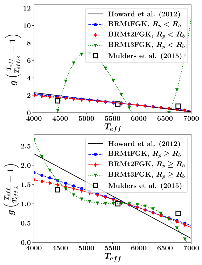
Visually comparing Figure 6 and Figure 11 show that the F, G, K type star data better reproduce the Howard et al. (2012) and Mulders et al. (2015a) results. Comparing Table 4 and Table 6 values show that the greatest differences in all of the parameters are in the coefficients. Comparing the SMM fit to the SMFGK fit and the SMAll fit shows a significant difference in the parameters. This indicates that the occurrence rate density function for M type stars must be different than F, G, and K type stars when considering only semi-major axis, planetary radius, and .
Our best-fit model is given as
| (13) |
where
| (14) |
and the numerical values are the 50th percentile values from the SMM and BRMt2FGK models. There is strong evidence that M type stars have more planets on short orbital periods (Mulders et al., 2015b; Burke et al., 2015) than F, G, and K type stars, so it is reasonable that occurrence rate density at 3900 K is piecewise continuous. Our analytical best fit model has the benefit that simple analytical conditional probability densities may be formed which allow planet samples to be generated quickly by Gibbs sampling (Gelfand & Smith, 1990) with self-written code or existing packages like BUGS (Lunn et al., 2009) or JAGS (Plummer, 2003). Sampling from published occurrence rates as in Barclay et al. (2018) requires an assumption of how planets are distributed within each bin (e.g. uniform or log-uniform), whereas sampling from our analytical best-fit model requires no such assumption.
6 Discussion
We now compare our model fits to literature data. Kopparapu et al. (2018) noted that combinations of SAG13 occurrence rate data tend to fall between Petigura et al. (2013a) at the low end and Burke et al. (2015) at the high end. The low end occurrence rate calculations from Petigura et al. (2013a) were based on an early and incomplete planet catalog. The high end occurrence rate calculations from Burke et al. (2015) considered many additional factors affecting occurrence rates and are more robust. We included the SAG13 data from Burke in our model fits, so we anticipate that our results derived from our model fits, will be close to those of Burke et al. (2015).
We first compare our fit results to Dressing & Charbonneau (2015) occurrence rates for M stars to highlight the break in the trend for stars with lower . Dressing & Charbonneau (2015) updated the results of Dressing & Charbonneau (2013) and gave slightly higher values for the occurrence rates. A comparison of our model fits to Dressing & Charbonneau (2015) is shown in Table LABEL:tab:dressing. We report the occurrence rates calculated at the 50th percentile model parameter values and include the 16th and 84th percentile values as our uncertainty estimate. The SMtAll model underpredicts the Dressing & Charbonneau (2015) occurrence rates by a factor between three and seven. The BRMtAll model performs better than the SMtAll model, but still underpredicts the Dressing & Charbonneau (2015) occurrence rates by a factor of two to five. The uncertainty levels of the SMM model overlap with those from Dressing & Charbonneau (2015) to give our best fit to the M type star data. This shows that the dependence on we assumed must have a break to accommodate M type stars with lower .
We compare our models to habitable zone occurrence rates reported by SAG13 and Burke et al. (2015). The habitable zone was calculated for a solar twin () from Kopparapu et al. (2013). These occurrence rates are given for a conservative (338–792 days or 0.95–1.68 AU) and an optimistic (237–864 days or 0.75–1.78 AU) estimate of the habitable zone. This comparison is shown in Table LABEL:tab:habitable. Our BRMt2FGK results are higher than the SAG13 and Burke et al. (2015) results but are still within the uncertainty ranges, thus showing agreement with these results.
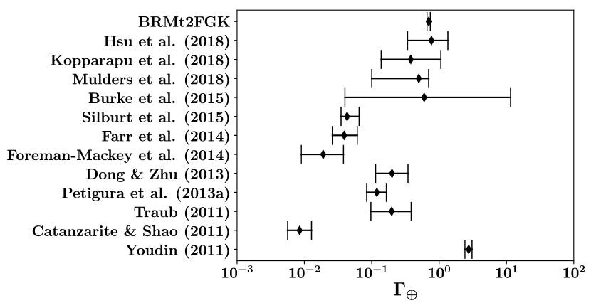
Our final comparison is to (Youdin, 2011; Foreman-Mackey et al., 2014; Burke et al., 2015) results from a number of studies where
| (15) |
We perform a change of variables to get our models in the proper form
| (16) |
For sun-like stars, this evaluates to
| (17) |
Figure 13 shows a comparison of our results to the literature and is similar to figures found in Foreman-Mackey et al. (2014) and one generated by Leslie Rogers (included in the SAG13 close-out presentation). We present results for our BRMt2FGK model. The error bars for our model are based on the 16% and 84% values of . The values from Hsu et al. (2018) when scaled to the appropriate units are . The Kopparapu et al. (2018) values are the reported which represent the SAG13 baseline, pessimistic, and optimistic cases. The values from Mulders et al. (2018) reflect the 1 values from the fitted parameters. The values from Burke et al. (2015) represent the allowable range. The Foreman-Mackey et al. (2014) values are the reported values. The Dong & Zhu (2013) values come from an extrapolation of the 1–2 fits where the error bars are given by the 1 values reported in their Table 2 and scaled to the appropriate units. The Petigura et al. (2013a) values reflect the reported . The Traub (2011) values come from an extrapolation of Equation 2 (including the factor ) and the error bars come from Traub (2011) Equation 6 and Equation 7. The Catanzarite & Shao (2011) values come from an extrapolation of the power law fit to period and the error bars reflect the 1 values on the power law index. The values from Youdin (2011) are the reported .
We see that from the BRMt2FGK model compares favorably with the values from Hsu et al. (2018), Kopparapu et al. (2018), Mulders et al. (2018), and Burke et al. (2015) and is well within the allowable range. All of the ranges from the literature fall within the allowable range of Burke et al. (2015) except for the ranges from Foreman-Mackey et al. (2014) and Catanzarite & Shao (2011). Burke et al. (2015) noted that there is overlap in the upper tail of from Foreman-Mackey et al. (2014) to the allowable range. Foreman-Mackey et al. (2014) used the same inputs as Petigura et al. (2013a) but found a steeper fall off of occurrence rates at longer periods. Foreman-Mackey et al. (2014) also found that accounting for uncertainty on planet radii led to a systematically lower value than Petigura et al. (2013a). Burke et al. (2015) noted that further work is needed to determine whether the differences between the Foreman-Mackey et al. (2014) result and the others from the literature come from differing inputs or methodology. Catanzarite & Shao (2011) fit a power law model on orbital period for occurrence rate data for 2–4 planets with periods up to 132 days. The values reported here come from their single power law fit and extrapolated to a planetary radius (unaccounted for in their power law model on period) of and period of one year. Because we extrapolate both planetary radius and period to get , it is understandable that Catanzarite & Shao (2011) is an outlier.
Our result shows the smallest error bars on because the only source of uncertainty from our model fits reduced to Equation 17 is in the term. The set up of our models was specifically chosen (transforming values to where results in ) to be most accurate for sun-like stars. When including the 16th and 84th percentile values for the BRMt2FGK model , , and . Although we sampled the posterior distribution of , these values show that propagating to results in narrow 1 error bars.
7 Conclusions
We have presented models for planet occurrence rate density based on previous occurrence rate calculations consisting of power laws on semi-major axis and planetary radius and a polynomial function of stellar . We found that M type stars do not follow the same relation on as F, G, and K type stars. We found that the best model fit to the M type star data was the SMM model, a power law on semi-major axis and planetary radius. We found that the best model fit to the F, G, and K type star data was the BRMt2FGK model, power laws broken at 2.771 with a quadratic function of . Our models give occurrence rates that are comparable with other published results and explicitly include stellar effective temperature as a variable. By explicitly including stellar effective temperature in our models, we are able to fit a wider range of occurrence rate data than previously published models.
By including more than just planetary physical and orbital parameters, our models are a step toward a more complete model of planet occurrence rates. The next step will be to create a model including additional stellar parameters which affect occurrence rates. Using our models in mission simulation or science yield calculations will give more accurate occurrence rates for individual stars by considering their individual stellar effective temperatures in the generation of planet samples instead of treating all stars the same. This will lead to more accurate science yield estimations for future and proposed exoplanet finding missions like HabEx and LUVOIR.
References
- Barclay et al. (2018) Barclay, T., Pepper, J., & Quintana, E. V. 2018, arXiv preprint arXiv:1804.05050
- Batalha (2014) Batalha, N. M. 2014, Proceedings of the National Academy of Sciences, 111, 12647
- Beaugé & Nesvornỳ (2012) Beaugé, C., & Nesvornỳ, D. 2012, The Astrophysical Journal, 763, 12
- Berger et al. (2018) Berger, T. A., Huber, D., Gaidos, E., & van Saders, J. L. 2018, arXiv preprint arXiv:1805.00231
- Berta et al. (2013) Berta, Z. K., Irwin, J., & Charbonneau, D. 2013, The Astrophysical Journal, 775, 91
- Biller et al. (2013) Biller, B. A., Liu, M. C., Wahhaj, Z., et al. 2013, The Astrophysical Journal, 777, 160
- Borucki (2017) Borucki, W. J. 2017, Proceedings of the American Philosophical Society, 161, 38
- Bowler & Nielsen (2018) Bowler, B. P., & Nielsen, E. L. 2018, arXiv preprint arXiv:1802.10132
- Brandt et al. (2014) Brandt, T. D., McElwain, M. W., Turner, E. L., et al. 2014, The Astrophysical Journal, 794, 159
- Brown (2005) Brown, R. A. 2005, The Astrophysical Journal, 624, 1010
- Brown & Soummer (2010) Brown, R. A., & Soummer, R. 2010, The Astrophysical Journal, 715, 122
- Bryan et al. (2016) Bryan, M. L., Knutson, H. A., Howard, A. W., et al. 2016, The Astrophysical Journal, 821, 89
- Buchhave et al. (2012) Buchhave, L. A., Latham, D. W., Johansen, A., et al. 2012, Nature, 486, 375
- Burke & Catanzarite (2017) Burke, C., & Catanzarite, J. 2017, Kepler Science Document, Tech. rep., KSCI-19111-002 ed RH Michael and MB Natalie
- Burke et al. (2015) Burke, C. J., Christiansen, J. L., Mullally, F., et al. 2015, The Astrophysical Journal, 809, 8
- Catanzarite & Shao (2011) Catanzarite, J., & Shao, M. 2011, The Astrophysical Journal, 738, 151
- Chen & Kipping (2016) Chen, J., & Kipping, D. 2016, The Astrophysical Journal, 834, 17
- Christiansen (2017) Christiansen, J. L. 2017, Kepler Science Document, KSCI-19110-001, Edited by Michael R. Haas and Natalie M. Batalha
- Christiansen et al. (2015) Christiansen, J. L., Clarke, B. D., Burke, C. J., et al. 2015, The Astrophysical Journal, 810, 95
- Clanton & Gaudi (2014) Clanton, C., & Gaudi, B. S. 2014, The Astrophysical Journal, 791, 91
- Clanton & Gaudi (2016) —. 2016, The Astrophysical Journal, 819, 125
- Coughlin (2017) Coughlin, J. L. 2017, Kepler Science Document, KSCI-19114-002, Edited by Natalie Batalha and Michael R. Haas
- Cumming et al. (2008) Cumming, A., Butler, R. P., Marcy, G. W., et al. 2008, Publications of the Astronomical Society of the Pacific, 120, 531
- Dong & Zhu (2013) Dong, S., & Zhu, Z. 2013, The Astrophysical Journal, 778, 53
- Dressing & Charbonneau (2013) Dressing, C. D., & Charbonneau, D. 2013, The Astrophysical Journal, 767, 95
- Dressing & Charbonneau (2015) —. 2015, The Astrophysical Journal, 807, 45
- Foreman-Mackey (2016) Foreman-Mackey, D. 2016, The Journal of Open Source Software, 2016
- Foreman-Mackey et al. (2013) Foreman-Mackey, D., Hogg, D. W., Lang, D., & Goodman, J. 2013, Publications of the Astronomical Society of the Pacific, 125, 306
- Foreman-Mackey et al. (2014) Foreman-Mackey, D., Hogg, D. W., & Morton, T. D. 2014, The Astrophysical Journal, 795, 64
- Fressin et al. (2013) Fressin, F., Torres, G., Charbonneau, D., et al. 2013, The Astrophysical Journal, 766, 81
- Fulton et al. (2017) Fulton, B. J., Petigura, E. A., Howard, A. W., et al. 2017, The Astronomical Journal, 154, 109
- Garrett & Savransky (2016) Garrett, D., & Savransky, D. 2016, The Astrophysical Journal, 828, 20
- Gelfand & Smith (1990) Gelfand, A. E., & Smith, A. F. 1990, Journal of the American statistical association, 85, 398
- Gonzalez (1997) Gonzalez, G. 1997, Monthly Notices of the Royal Astronomical Society, 285, 403
- Goodman & Weare (2010) Goodman, J., & Weare, J. 2010, Communications in applied mathematics and computational science, 5, 65
- Howard et al. (2010a) Howard, A. W., Marcy, G. W., Johnson, J. A., et al. 2010a, Science, 330, 653
- Howard et al. (2010b) Howard, A. W., Johnson, J. A., Marcy, G. W., et al. 2010b, The Astrophysical Journal, 721, 1467
- Howard et al. (2012) Howard, A. W., Marcy, G. W., Bryson, S. T., et al. 2012, The Astrophysical Journal Supplement Series, 201, 15
- Hsu et al. (2018) Hsu, D. C., Ford, E. B., Ragozzine, D., & Morehead, R. C. 2018, The Astronomical Journal, 155, 205
- Huber et al. (2014) Huber, D., Aguirre, V. S., Matthews, J. M., et al. 2014, The Astrophysical Journal Supplement Series, 211, 2
- Jenkins (2017) Jenkins, J. M. 2017, Kepler Science Document, KSCI-19081-002, Edited by Dwight Sanderfer, Michael R. Haas, and Natalie M. Batalha
- Kass & Raftery (1995) Kass, R. E., & Raftery, A. E. 1995, Journal of the american statistical association, 90, 773
- Kopparapu et al. (2013) Kopparapu, R. K., Ramirez, R., Kasting, J. F., et al. 2013, The Astrophysical Journal, 765, 131
- Kopparapu et al. (2018) Kopparapu, R. K., Hébrard, E., Belikov, R., et al. 2018, The Astrophysical Journal, 856, 122
- Lafreniere et al. (2007) Lafreniere, D., Doyon, R., Marois, C., et al. 2007, The Astrophysical Journal, 670, 1367
- Lee & Chiang (2017) Lee, E. J., & Chiang, E. 2017, The Astrophysical Journal, 842, 40
- Lunn et al. (2009) Lunn, D., Spiegelhalter, D., Thomas, A., & Best, N. 2009, Statistics in medicine, 28, 3049
- Marcy et al. (2005) Marcy, G., Butler, R. P., Fischer, D., et al. 2005, Progress of Theoretical Physics Supplement, 158, 24
- Mathur et al. (2017) Mathur, S., Huber, D., Batalha, N. M., et al. 2017, The Astrophysical Journal Supplement Series, 229, 30
- Mayor et al. (2011) Mayor, M., Marmier, M., Lovis, C., et al. 2011, arXiv preprint arXiv:1109.2497
- Morton & Swift (2014) Morton, T. D., & Swift, J. 2014, The Astrophysical Journal, 791, 10
- Mulders (2018) Mulders, G. D. 2018, in Handbook of Exoplanets, ed. H. J. Deeg & J. A. Belmonte (Cham: Springer International Publishing), 1–26. https://doi.org/10.1007/978-3-319-30648-3_153-1
- Mulders et al. (2015a) Mulders, G. D., Pascucci, I., & Apai, D. 2015a, The Astrophysical Journal, 798, 112
- Mulders et al. (2015b) —. 2015b, The Astrophysical Journal, 814, 130
- Mulders et al. (2018) Mulders, G. D., Pascucci, I., Apai, D., & Ciesla, F. J. 2018, The Astronomical Journal, 156, 20
- Mulders et al. (2016) Mulders, G. D., Pascucci, I., Apai, D., Frasca, A., & Molenda-Żakowicz, J. 2016, The Astronomical Journal, 152, 187
- Mullally et al. (2015) Mullally, F., Coughlin, J. L., Thompson, S. E., et al. 2015, The Astrophysical Journal Supplement Series, 217, 31
- Nielsen & Close (2010) Nielsen, E. L., & Close, L. M. 2010, The Astrophysical Journal, 717, 878
- Nielsen et al. (2008) Nielsen, E. L., Close, L. M., Biller, B. A., Masciadri, E., & Lenzen, R. 2008, The Astrophysical Journal, 674, 466
- Pascucci et al. (2018) Pascucci, I., Mulders, G. D., Gould, A., & Fernandes, R. 2018, The Astrophysical Journal Letters, 856, L28
- Pecaut & Mamajek (2013) Pecaut, M. J., & Mamajek, E. E. 2013, The Astrophysical Journal Supplement Series, 208, 9
- Petigura et al. (2013a) Petigura, E. A., Howard, A. W., & Marcy, G. W. 2013a, Proceedings of the National Academy of Sciences, 110, 19273
- Petigura et al. (2013b) Petigura, E. A., Marcy, G. W., & Howard, A. W. 2013b, The Astrophysical Journal, 770, 69
- Petigura et al. (2018) Petigura, E. A., Marcy, G. W., Winn, J. N., et al. 2018, The Astronomical Journal, 155, 89
- Plummer (2003) Plummer, M. 2003, in Proceedings of the 3rd International Workshop on Distributed Statistical Computing
- Reffert et al. (2015) Reffert, S., Bergmann, C., Quirrenbach, A., Trifonov, T., & Künstler, A. 2015, Astronomy & Astrophysics, 574, A116
- Santos et al. (2004) Santos, N. C., Israelian, G., & Mayor, M. 2004, Astronomy & Astrophysics, 415, 1153
- Savransky & Garrett (2015) Savransky, D., & Garrett, D. 2015, Journal of Astronomical Telescopes, Instruments, and Systems, 2, 011006
- Schlaufman (2018) Schlaufman, K. C. 2018, The Astrophysical Journal, 853, 37
- Schwarz et al. (1978) Schwarz, G., et al. 1978, The annals of statistics, 6, 461
- Silburt et al. (2015) Silburt, A., Gaidos, E., & Wu, Y. 2015, The Astrophysical Journal, 799, 180
- Sousa et al. (2008) Sousa, S., Santos, N., Mayor, M., et al. 2008, Astronomy & Astrophysics, 487, 373
- Spergel et al. (2015) Spergel, D., Gehrels, N., Baltay, C., et al. 2015, arXiv preprint arXiv:1503.03757
- Stark et al. (2014) Stark, C. C., Roberge, A., Mandell, A., & Robinson, T. D. 2014, The Astrophysical Journal, 795, 122
- Tabachnik & Tremaine (2002) Tabachnik, S., & Tremaine, S. 2002, Monthly Notices of the Royal Astronomical Society, 335, 151
- Thompson et al. (2018) Thompson, S. E., Coughlin, J. L., Hoffman, K., et al. 2018, The Astrophysical Journal Supplement Series, 235, 38. http://stacks.iop.org/0067-0049/235/i=2/a=38
- Traub (2011) Traub, W. A. 2011, The Astrophysical Journal, 745, 20
- Traub (2016) —. 2016, arXiv preprint arXiv:1605.02255
- Valenti & Fischer (2005) Valenti, J. A., & Fischer, D. A. 2005, The Astrophysical Journal Supplement Series, 159, 141
- Vigan et al. (2017) Vigan, A., Bonavita, M., Biller, B., et al. 2017, Astronomy & Astrophysics, 603, A3
- Wahhaj et al. (2013) Wahhaj, Z., Liu, M. C., Nielsen, E. L., et al. 2013, The Astrophysical Journal, 773, 179
- Weiss & Marcy (2014) Weiss, L. M., & Marcy, G. W. 2014, The Astrophysical Journal Letters, 783, L6
- Wilson et al. (2018) Wilson, R. F., Teske, J., Majewski, S. R., et al. 2018, The Astronomical Journal, 155, 68
- Winn (2018) Winn, J. N. 2018, arXiv preprint arXiv:1801.08543
- Winn & Fabrycky (2015) Winn, J. N., & Fabrycky, D. C. 2015, Annual Review of Astronomy and Astrophysics, 53
- Wolfgang et al. (2016) Wolfgang, A., Rogers, L. A., & Ford, E. B. 2016, The Astrophysical Journal, 825, 19
- Youdin (2011) Youdin, A. N. 2011, The Astrophysical Journal, 742, 38
- Zhu et al. (2016) Zhu, W., Wang, J., & Huang, C. 2016, The Astrophysical Journal, 832, 196