AMICO galaxy clusters in KiDS-DR3: sample properties and selection function
Abstract
We present the first catalogue of galaxy cluster candidates derived from the third data release of the Kilo Degree Survey (KiDS-DR3). The sample of clusters has been produced using the Adaptive Matched Identifier of Clustered Objects (AMICO) algorithm. In this analysis AMICO takes advantage of the luminosity and spatial distribution of galaxies only, not considering colours. In this way, we prevent any selection effect related to the presence or absence of the red-sequence in the clusters. The catalogue contains candidate galaxy clusters in the redshift range down to with a purity approaching % over the entire redshift range. In addition to the catalogue of galaxy clusters we also provide a catalogue of galaxies with their probabilistic association to galaxy clusters. We quantify the sample purity, completeness and the uncertainties of the detection properties, such as richness, redshift, and position, by means of mock galaxy catalogues derived directly from the data. This preserves their statistical properties including photo- uncertainties, unknown absorption across the survey, missing data, spatial correlation of galaxies and galaxy clusters. Being based on the real data, such mock catalogues do not have to rely on the assumptions on which numerical simulations and semi-analytic models are based on. This paper is the first of a series of papers in which we discuss the details and physical properties of the sample presented in this work.
keywords:
galaxies: clusters: general – cosmology: observations – large-scale structure of Universe1 Introduction
clusters of galaxies are one of the fundamental probes to study the nature of dark matter and dark energy (Umetsu et al., 2014; Planck Collaboration et al., 2016b; Sartoris et al., 2016; de Haan et al., 2016; Wang et al., 2016; Smith et al., 2016; Giocoli et al., 2018; Schellenberger & Reiprich, 2017; Corasaniti et al., 2018), gravity itself (Llinares & Mota, 2013; L’Huillier et al., 2017), to constrain neutrino masses (Costanzi et al., 2013; Roncarelli et al., 2015) as well as the far universe and the early stages of star and galaxy formation when used as gravitational lensing telescopes (Zheng et al., 2012; Coe et al., 2013; Bradley et al., 2014; Kelly et al., 2015; Rydberg et al., 2018). There are many ways to identify galaxy clusters: through the X-ray emission (Böhringer et al., 2004; Pace et al., 2008; Piffaretti et al., 2011; Merloni et al., 2012; Clerc et al., 2014), the comptonization of the Cosmic Microwave Background photons by the hot plasma they contain (Reichardt et al., 2013; Planck Collaboration et al., 2016a; Hilton et al., 2018), the gravitational lensing distortion they induce on background galaxies (Maturi et al., 2005; Pace et al., 2007; Bellagamba et al., 2011) and the optical emission of their population of galaxies. Various methods have been proposed and used for their detection in photometric catalogue of galaxies. For instance wavelength filters (Gonzalez, 2014; Benoist, 2014), friend-of-friends (Farrens et al., 2011), methods based on Voronoi tessellation (Iovino, 2014), minimal spanning trees (Adami & Mazure, 1999), red-sequenced finders (Rykoff et al., 2014; Licitra et al., 2016) and matched optimal filters (Bellagamba et al., 2011; Bellagamba et al., 2018, Adam et al. in prep.).
In this work, we searched for galaxy clusters in the third data release of the Kilo Degrees Survey (KiDS-DR3, de Jong et al., 2017). With respect to our previous study on the second data release (Radovich et al., 2016, 2017), the analysis presented here benefits of a larger survey area, better data quality, and significant improvements in the cluster detection algorithm. For this task we use the Adaptive Matched Identifier of Clustered Objects algorithm (AMICO, Bellagamba et al., 2018), an optimal matched filter which takes advantage of the known statistical properties of the field galaxies and of galaxy clusters. Even if AMICO can deal with an arbitrary number of quantities describing galaxies, in this specific application we consider their spatial coordinates, magnitude, and photo- only. We deliberately avoided the use of their colors to aim at a selection function minimally sensitive to the presence (or absence) of the red-sequence of clusters.
To derive the uncertainty on the properties of the detections, the purity and the completeness of the sample we realized a series of realistic mock catalogues of galaxies based on the real KiDS data. In doing so, we took care to preserve the actual masked areas in the data, all photometric and photo- properties of the galaxies, as well as their large scale correlation and the correlation of clusters among themselves and inside large scale structures.
The structure of the paper is as follows. In Section (2) we describe the data set. In Section (3) we summarize the characteristics of the detection algorithm and the new features used specifically for this work. The catalogue of galaxy clusters and the comparison with existing catalogues are presented in Sections (4) and (5), respectively. The uncertainties on the detection properties, the completeness and purity of the sample are quantified in Section (6). Finally the conclusions are summarized in Section (7).
2 The data sets
We analysed the galaxy catalogue coming from the KiDS Data Release 3 (de Jong et al., 2017) obtained with the OmegaCAM wide-field imager (Kuijken, 2011) mounted at the VLT Survey Telescope, a 2.6m telescope sited at the Paranal Observatory (VST; Capaccioli & Schipani, 2011). OmegaCAM contains a mosaic of 32 science CCDs offering a field of view of 1 deg2 with a resolution of 0.21 arcsec/pixel. The data cover an area of about 440 split into two main stripes, one equatorial (KiDS-N) and one centred around the South Galactic Pole (KiDS-S). The galaxy catalogue provides the coordinates, the 2 arcsec aperture photometry in four bands (u, g, r, i) and photometric redshifts for all galaxies down to the limiting magnitudes of 24.3, 25.1, 24.9 and 23.8 in the four bands, respectively. We selected all galaxies with magnitude for a total of about million objects.
The photometric redshifts of the galaxies have been obtained with BPZ, a Bayesian photo- estimator based on a template-fitting method (Benítez, 2000; de Jong et al., 2017). BPZ returns a photo- posterior probability distribution function which is fully exploited by AMICO (see below). Other two sets of photometric redshifts obtained via Machine-Learning techniques, MLPQNA and ANNz2, are available in KiDS-DR3 (de Jong et al., 2017; Bilicki et al., 2018). An extensive analysis of the probability distribution functions derived for these two sets will be presented in Amaro et al (2018): since it was still in progress when our cluster catalog was derived, we opted to use the well tested BPZ photometric redshifts. In next releases we will also investigate the usage of Machine-Learning photometric redshifts.
3 AMICO: the detection algorithm
For the detection of the galaxy clusters we used the AMICO code (Bellagamba et al., 2018). In this section we briefly summarize its main concepts and the features recently implemented and adopted in the following analysis.
3.1 Linear optimal matched filtering
AMICO is based on a linear optimal matched filter approach (Maturi et al., 2005, 2007; Viola et al., 2010; Bellagamba et al., 2011). Within this framework, the data, , are modelled as the superimposition of the signal we are interested in, i.e. the galaxy clusters signal , and a noise component, , describing the contamination given by the field galaxies. The filter itself is a kernel used to convolve the data and it is derived through a constrained minimization procedure aiming at estimating the signal amplitude, , which is unbiased and with minimum variance. Despite the fact AMICO can deal with an arbitrary number of galaxy properties we restrict ourself to the simple case in which the data points, , are individual galaxies, labelled with , characterized by sky coordinates, , an r-band magnitude, , and a photometric redshift distribution, . The aforementioned convolution returning an estimate for is evaluated on a three-dimensional grid (,), with resolution of across the sky and in redshift, and is discretized to deal with counts of galaxies:
| (1) |
Here, and describe the properties of the field and cluster galaxies at redshift , respectively, as it will be detailed in Section (3.4); the factor takes care of the filter normalization and is a background subtraction term quantifying the average contribution of the field galaxies to the total signal amplitude. The expected r.m.s. of the amplitude is given by
| (2) |
where the first term refers to the stochastic fluctuations of the background and the second one is related to the Poissonian fluctuations given by the galaxies of a cluster with amplitude . The factors , , and are properties of the filter and solely depend on the cluster111We base the redshift distribution of the model on the average of the input galaxies as detailed in Bellagamba et al. (2018). and field models. The definition of is given in Bellagamba et al. (2018), while the new definitions of and , implementing the new features of the algorithm, are given in Section (3.2).
Once the amplitude has been evaluated for all angular and redshift positions, the first cluster candidate is then identified as the location with the largest likelihood,
| (3) |
and positive amplitude. Here, is a constant of no relevance that we no further discuss. With a cluster detection at hand, labelled with , we evaluate the probability of all galaxies in that region of being its members,
| (4) |
Here,
| (5) |
is the probability of the -th galaxy to belong to the field. In general, a galaxy can be associated to more detections because they can overlap. We store the information of all cluster members down to a membership probabilistic association of .
To proceed with the search of further clusters, we remove from the amplitude map the contribution of the last found detection, re-evaluate the likelihood and variance to finally identify a new candidate as done with the previous one. The removal of a detection is done by taking advantage of the membership probabilistic association of the galaxies to a detection, , as follows
| (6) |
This signal subtraction facilitates a better identification of objects which might be blended with those with larger amplitudes. We refer to this process as “cleaning”. This iterative process proceeds down to a desired minimum signal-to-noise ratio, , that in this work is set to .
| name | description |
|---|---|
| amplitude, natural output of the filter | |
| apparent richness, number of visible galaxies | |
| intrinsic richness, as but for and |
3.2 New features of the algorithm
In order to correctly normalise the amplitude and estimate its uncertainty , AMICO calculates the quantities and , which depend on the properties of the redshift probability distributions of the galaxy sample. In Bellagamba et al. (2018), this was done by introducing , the typical redshift probability distribution for a galaxy which lies at redshift , computed as
| (7) |
where is the most probable redshift for the -th galaxy. In this analysis, we refined this treatment in two ways. First of all, we computed the photo- properties as a function of the -band magnitude to capture the different precision of photo-s depending on the quality of the galaxy photometry. Then, we replaced with two different statistics and defined by
| (8) |
and
| (9) |
where means that the sum runs only on the galaxies whose peak corresponds to . In practice, describes the typical that peaks at , while describes the probability distribution for the peak, , of a galaxy that is located at redshift . Together, they allow to measure the typical precision of the redshift probability distribution as a function of , but also the small-scale features of the -peaks distribution, removing the smoothing that is implicit in Equation (7). With these two new quantities, the constants and can be now defined as
| (10) |
and
| (11) |
3.3 Mass proxies and cluster richness
As discussed in Section (3.1), the natural output of the linear optimal matched filter is the amplitude, , expressed by Equation (6). In this Section, we derive two other mass proxies based on the probabilistic membership association of the galaxies to detections (Equation 4). The first one is the apparent richness that is defined as the sum of the probabilities of all galaxies associated to the detection,
| (12) |
This quantity represents the number of visible galaxies belonging to a detection. Clearly, this number depends on the cosmic distance at which a cluster is located so that is a redshift dependent quantity. In fact, the further the cluster, the smaller the number of visible members. The advantage of this definition with respect to the amplitude is that it is related to a direct observable, namely the number of visible galaxies.
The second mass proxy here used is the intrinsic richness defined in a similar fashion but by summing over the galaxies brighter than and within the virial radius, ,
| (13) |
The radial cut and are parameters of the model we used for the construction of the filter, see Section (3.4), that we adopt for internal consistency. Obviously each detection has its own and we could scale the radial cut-off with the detection amplitude or apparent richness , but this would lead to an additional stochastic scatter given by the uncertainty of these quantities. Note that these definitions depend on the conversion from angular to physical distances and therefore imply the assumption of a specific cosmological model222We assume a CDM cosmological model with , , through out the paper.. Despite that, is a nearly redshift independent quantity which can better characterize the clusters mass. This is because the threshold is well below the magnitude limit for the galaxy sample for the entire redshift range considered in this work. In Table (1), we list the mass proxies provided by AMICO and delivered with the catalogue of galaxy clusters.
3.4 Model description: cluster and field galaxies
The cluster model, , describes the expected galaxy distribution as a function of distance from the centre, , and -band magnitude, , for a cluster at redshift . In this work, the cluster model is constructed from a luminosity function and a radial profile as
| (14) |
where we made implicit the dependence on the redshift . The parameters for these distributions are taken from the analysis of a sample of Sunyaev Zel’dovich detected clusters observed by the Dark Energy Survey (DES; Hennig et al., 2017; Zenteno et al., 2016). These clusters cover a redshift range , which is broadly comparable to ours, and their detection via the Sunyaev Zel’dovich effect (SZ, hereafter) avoids any selection bias related to the optical properties of the galaxies in clusters, which could introduce systematics in the detection process.
In particular, the luminosity function follows a Schechter function (Schechter, 1976)
| (15) |
Note that we only use the shape of the distribution and not the normalization since the latter is absorbed by the constants during the filter construction. The typical magnitude as a function of redshift is derived from a stellar population evolutionary model with a decaying starburst at redshift = 3 (decay time = 0.4 Gyr) and a Chabrier initial mass function (IMF; Bruzual & Charlot, 2003). This model has been described and confirmed in DES data by Zenteno et al. (2016) where they also derived a mean faint-end slope of , which we adopt.
For the radial profile we assume an Navarro-Frenk-White profile (NFW; Navarro et al., 1997)
| (16) |
where the scale radius depends on the concentration via . Hennig et al. (2017) found the NFW distribution is a good description of the observed cluster profiles, with a mean = 3.59. For our cluster model we used this value and an corresponding to a mass = , typical for the cluster sample we want to target. The normalisation parameter is such that the total number of galaxies inside and below is coherent with the relation with found by Hennig et al. (2017). For a mass = , this corresponds to = 22.9.
The field galaxies distribution can be approximated by the total distribution in the galaxy sample, as the cluster component is small. For each redshift , we build weighing each galaxy with its redshift probability distribution .
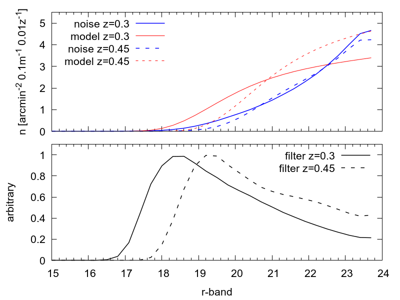
For illustration purposes, we show in the top panel of Figure (1) the luminosity function of both field galaxies and cluster members at redshift (solid lines) and (dashed lines). The magnitude dependence of the algorithm filter resulting from the use of these luminosity functions is shown in the bottom panel of the same figure. Such filter turns out to be a band-pass filter with gives more weight to the galaxies with a certain luminosity on the bright end side, the higher the redshift, the larger the magnitude which the filter peaks at.
4 Clusters detectitons and galaxy members
In this section we describe the catalogue of galaxy clusters detected in the KiDS-DR3 with the AMICO code. We provide the main statistical properties of the sample and present few examples of detections.
4.1 The catalog of galaxy clusters
The survey covers a total area of deg2 but we rejected all galaxies falling in those regions severely affected by satellite tracks, haloes produced by bright stars, and image artefacts in general, leaving us with deg2 (“Primary halo” masks, see de Jong et al., 2015). The remaining galaxies have been used to produce an initial set of detections down to as explained in Section (3). This first sample of detections has been then filtered out by rejecting all objects falling in the more restrictive masks used for the weak lensing analysis (“Secondary/tertiary halo” masks, see de Jong et al., 2015). The final effective area is of deg2, i.e. % of the total area of the survey. All detections with have been used for the construction of the mock simulations discussed in Section (6.1), but for the final catalogue of clusters we kept only those with obtaining a final sample with objects333The catalogue is available on request.. This buffer in is necessary for constructing reliable mock catalogues and derive solid statistical properties for our cluster sample as it will be detailed in Section (6.1.2). The entries of the catalogue are specified in Table (3). For all 6972 objects falling in the redshift range , we also provide mass estimates obtained via stacked weak-gravitational lensing (Bellagamba et al. submitted).
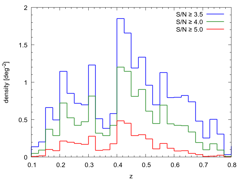
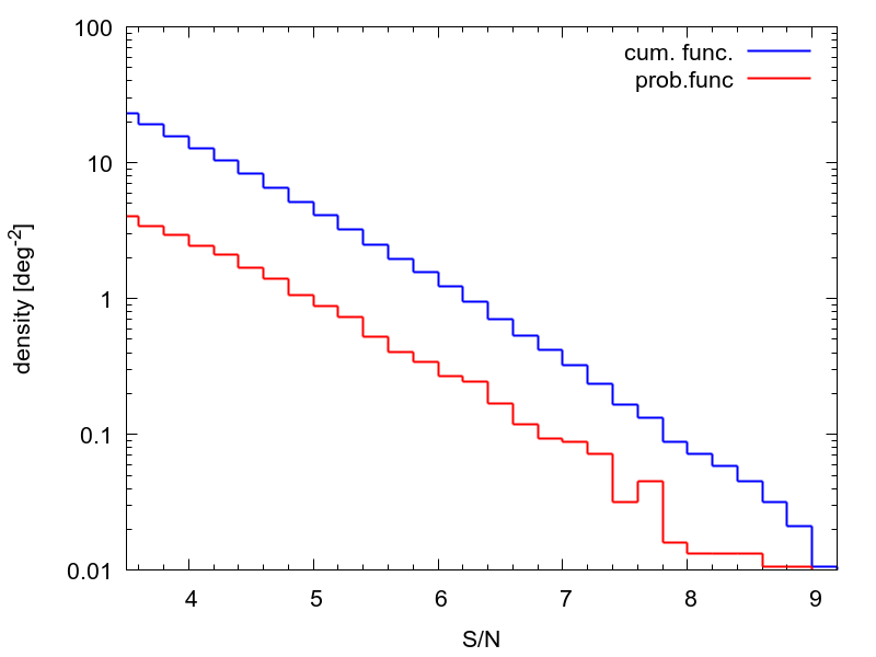
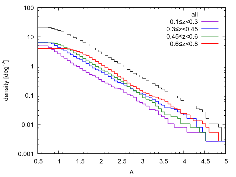
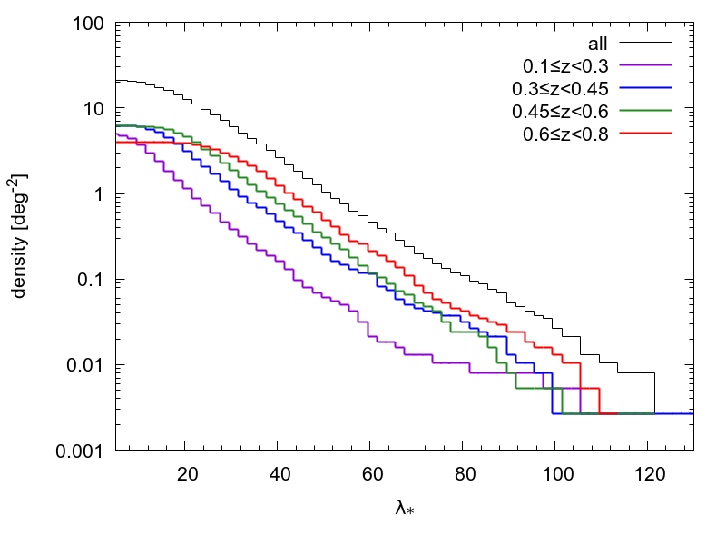
In Figure (2) we summarize the main statistical properties of the detections listed in the catalogue by showing their number density as a function of redshift (top left panel), signal-to-noise ratio (top right panel), amplitude and intrinsic richness (left and right bottom panels, respectively). The drop in density at is due to problems in the returned photometric redshift due to the shape of the g and r filters, resulting in a not optimal covering of the break at that redshift (see e.g., Padmanabhan et al., 2005).
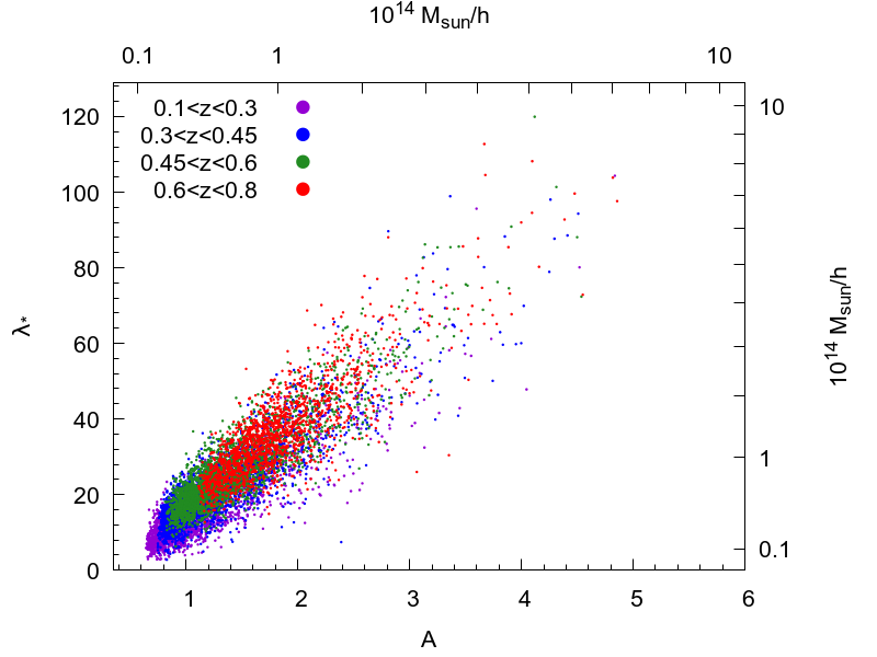
Finally, Figure (3) shows the amplitude against the intrinsic richness for the galaxy clusters falling in four different redshift bins. The mass indicated on the secondary axes is derived from the scaling relations of and based on weak-lensing measurements and based on a fiducial value of (Bellagamba et al. submitted). We can safely show the mass based on a scaling relation computed at a specific redshift because of its small redshift dependence.
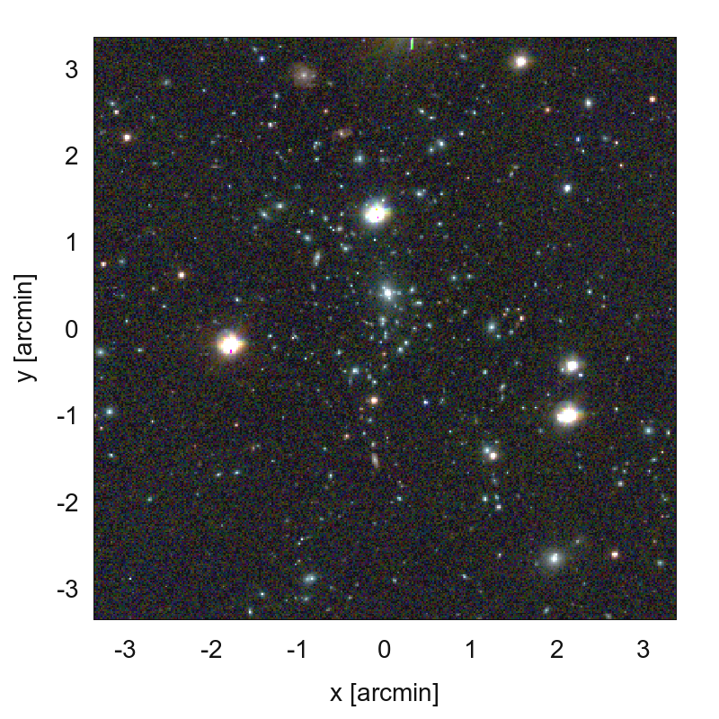
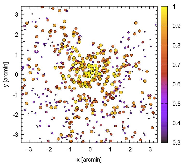
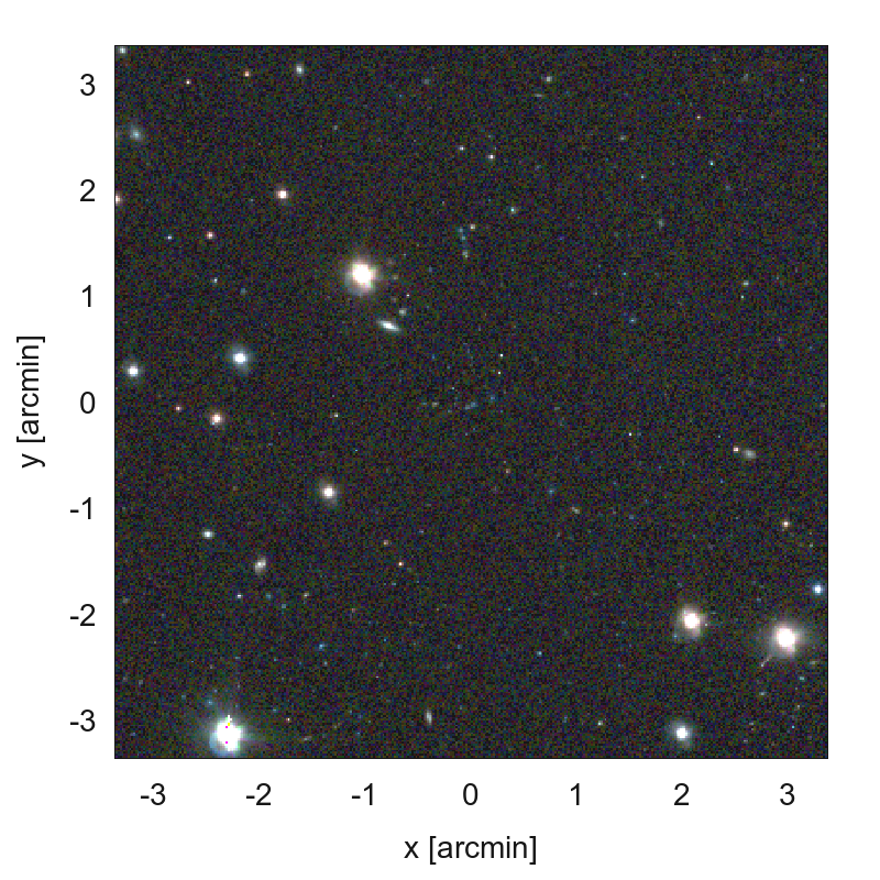
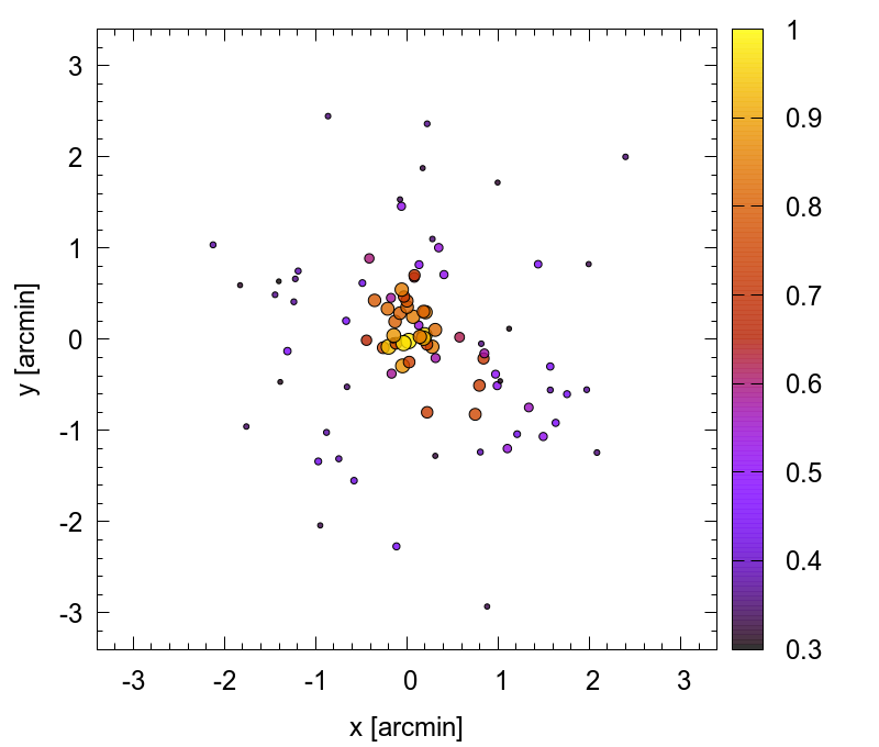
As an example of detections, we show in the left panels of Figure (4) the image cut-outs of a rich cluster, with , at relatively low redshift, , and an intermediate one, with , at a higher redshift, . The first cluster has been detected with while the second one with . Both cut-outs are of arcsec in size. In the corresponding right panels we show how the AMICO code “sees” the same two clusters. The circles mark the position of the galaxies visible in the image cut-outs with size and color related to their probabilistic association to the detection. The plot shows clearly the depenence of membership probabilistic association with the angular distance from the detection center. However, the value of has also a dependence on magnitude and on the of the galaxy (see eq. 4). Other examples are shown in Appendix (A).
4.2 The catalogue of cluster members
As discussed in Section (3.1), AMICO returns a probabilistic association of galaxies to cluster candidates, see Equatiton (4). Using this information, we present a catalogue of cluster members with a maximum of twenty associations to clusters, labelled with , as well as their probability to be field galaxies, . We note that in the catalogue we do not apply any cut in membership probability. This catalogue can be used to study the properties of clusters, galaxy formation, help in the removal of the foreground for weak-lensing studies, improve the strong lensing estimates derived with photometric based algorithms (Stapelberg et al., 2017; Carrasco et al., 2018), among many other applications.
5 Correlation with other data sets
In this section we compare our sample with other catalogues of galaxy clusters published in the literature. A positive match between one of our detections and one of the other entries occurs if they lay within and Mpc/h one from the other.
5.1 RedMaPPer optically-selected clusters
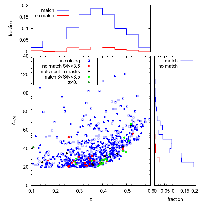
We compared our detections with the cluster candidates listed in Rykoff et al. (2014). This catalogue has been obtained by running the redMaPPer algorithm on the Sloan Digital Sky Survey Data Release 8 (SDSS-DR8) and contains entries within the redshift range . Of the 681 detections falling in the un-masked regions of KiDS-DR3 data, 624, i.e. , find a match. Of the remaining 57 detections, 20 have been detected by AMICO with a signal-to noise ratio in the range below our restrictive threshold of , while other 13 satisfy the matching criteria but lay inside a KiDS masked area. The remaining 24, i.e. less then of the redMaPPer sample, do not have a counterpart with . These redMaPPer cluster candidates have a richness measured by redMaPPer, , close to the detection limit of this algorithm as illustrated in Figure (5). Since the KiDS and the SDSS data sets are very different in terms of depth and image quality, no further comparison would be meaningful.
| ID | RA | DEC | ID | RA | DEC | z |
|---|---|---|---|---|---|---|
| 11 | 358.351 | -33.2932 | 7485 | 358.385 | -33.2837 | 0.67 |
| 19 | 350.538 | -34.5752 | 6948 | 350.468 | -34.6173 | 0.23 |
| 39 | 354.054 | -32.1343 | 7226 | 354.053 | -32.1320 | 0.41 |
| 41 | 342.976 | -33.3942 | 6473 | 342.963 | -33.4027 | 0.24 |
| 44 | 356.853 | -31.1509 | 7361 | 356.884 | -31.1470 | 0.45 |
| 48 | 341.633 | -32.2011 | 6295 | 341.717 | -32.2280 | 0.50 |
| 50 | 351.169 | -30.6511 | 7002 | 351.156 | -30.6723 | 0.31 |
| 59 | 340.637 | -30.3150 | 6241 | 340.618 | -30.4084 | 0.24 |
| 1033 | 39.6692 | -30.8391 | 7601 | 39.6215 | -30.8968 | 0.55 |
| 1606 | 216.108 | -2.73976 | 4120 | 216.089 | -2.83463 | 0.77 |
5.2 Planck SZ-selected clusters
Of all clusters listed in the second Planck catalogue of Sunyaev-Zeldovich sources (Planck Collaboration et al., 2016a), 19 fall in the area we processed and all of them have been detected by AMICO. The redshift of 10 of these objects has not been reported in the literature to our knowledge and for this we list in Table (2) our estimate as measured with the AMICO code. Note that the cluster with ID has not been detected with redMaPPer because located at a redshift, , which exceeds their maximum limit.
5.3 MCXC X-ray selected clusters
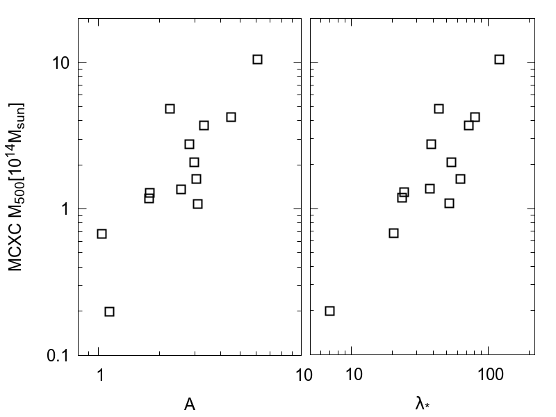
We then compared our mass proxies with the X-rays mass estimates listed in the Meta-Catalog of X-ray detected Clusters of galaxies (MCXC; Piffaretti et al., 2011). The MCXC catalogue comprises X-rays selected clusters collected in archival data and includes the ROSAT All Sky Survey-based (NORAS, REFLEX, BCS, SGP, NEP, MACS, and CIZA) and serendipitous cluster catalogues (160SD, 400SD, SHARC, WARPS, and EMSS) for a total of 1743 objects. Since the data have been taken with different instruments and exposure times, they have been homogenized in order to provide a coherent picture for this sample. All 13 clusters of the MCXC catalogue falling in the KiDS-DR3 foot-print have been identified by AMICO. In Figure (6) we compare our two mass proxies, and , with the value of derived with the X-Rays observations. A well defined correlation is evident.
5.4 GAMA spectroscopy
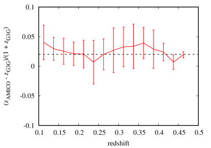
We finally used the GAMA-I galaxy group catalogue (G3C; Driver et al., 2009, 2011; Liske et al., 2015) to verify the redshift estimate of the clusters provided by the AMICO code. GAMA is a highly complete spectroscopic survey up to a Petrosian r-band magnitude of and comprises galaxies, of which belong to galaxy groups identified with a friends-of-friends (FoF) algorithm in the redshift range (Robotham et al., 2011). In Figure (7) we plot the relative scatter between the redshift estimates of the groups as measured by AMICO and those listed in the G3C catalogue. A clear bias, well described by , emerges from this comparison. This bias corresponds to what was found by de Jong et al. (2017) when comparing KiDS photo-zs with GAMA spec-z (See their table 8). Since the sample of the G3C is limited to , we can not draw any conclusions for clusters at higher redshifts. More details regarding this bias and how we deal with it will be given in Section (6.2) together with an extensive discussion of all other uncertainties.
6 Assessing the quality of the detections
In this section, we describe a method to produce realistic mock catalogues, constructed from the real data themselves, that we use to estimate the uncertainties of the quantities characterizing the detections as well as the purity and completeness of the entire sample.
6.1 Mock simulations
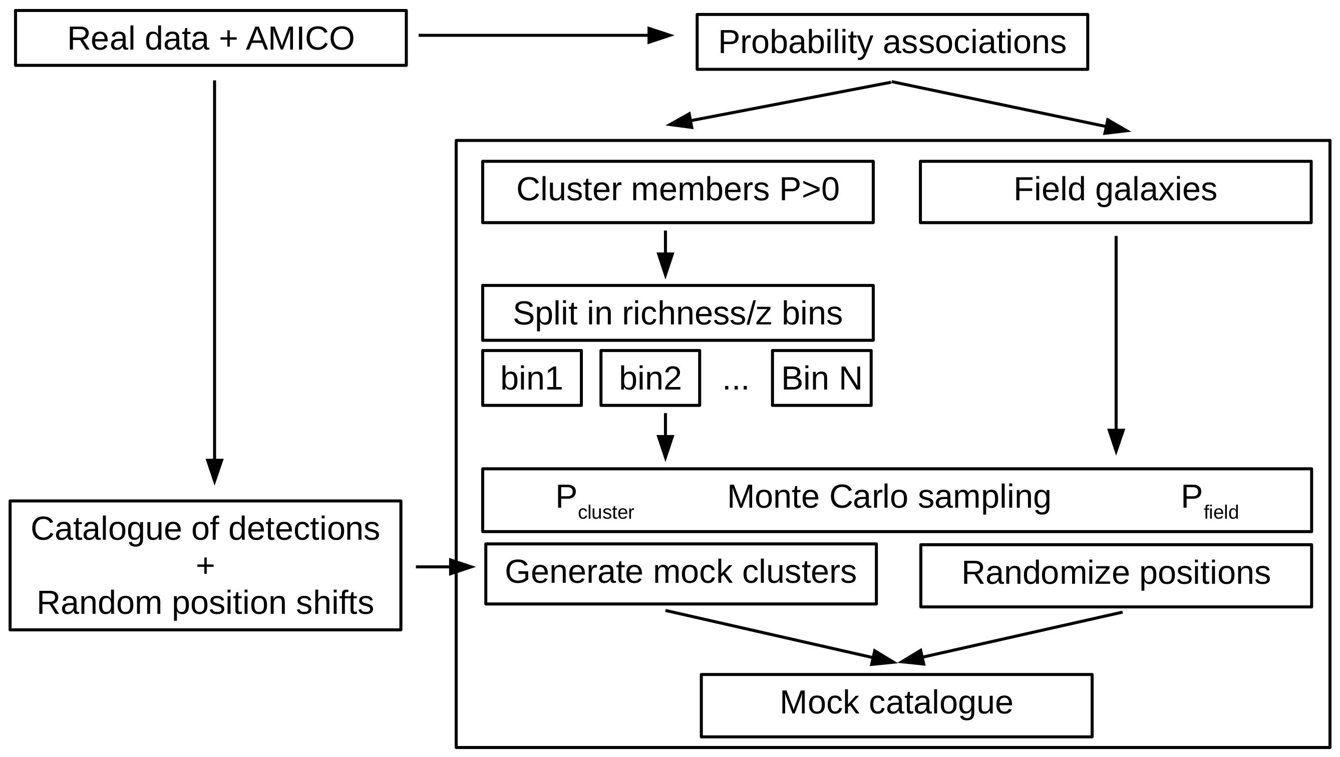
We base our mocks on the original KiDS-DR3 data rather then on numerical simulations to minimize the number of assumptions and to account for all expected and unexpected properties of the survey across the sky, such as photometric and phot-z uncertainties, absorption, masks, variation in depth as well as the clustering of galaxies etc. The central idea of the mocks rely on a Monte Carlo extraction of the galaxies based on their probabilistic association to the entries in our cluster sample, Equation (4), and to the field, Equation (5). A scheme with all steps involved in the mock generation is shown in Figure (8).
In the following, we describe the procedure to create the mock field population, Section (6.1.1), and the mock clusters, Section (6.1.2). We will discuss several aspects related to the methodology in Section (6.1.3).
6.1.1 Mock field galaxies
The field galaxies are extracted from the KiDS data catalogue via a Monte Carlo sampling based on the probability, . In detail, for each galaxy we extract a uniform random number between 0 and 1, and assign the galaxy to the field if . For example, a galaxy with has the chance to be extracted and associated to the field. All observed properties of these galaxies are preserved except for their position in the sky which is slightly perturbed by introducing a random angular displacement. The maximum random displacement is a free parameter which we set to Mpc/h. This scale is large enough to dump the presence of clusters which might have not been detected by the algorithm but is small enough to preserve the correlation of the Large Scale Structures (LSS).
6.1.2 Mock galaxy clusters
To generate the mock clusters we started by defining bins of apparent richness and redshift in which to collect all galaxies associated to clusters. All galaxies with have been considered and those with more than one cluster association have been attributed to more than one bin accordingly. In this way, each bin contains all galaxies potentially belonging to clusters with the richness and redshift defining the bin itself. Each mock cluster is then generated by randomly extracting galaxies out of the corresponding bin via a Monte Carlo sampling based on their cluster membership probability (see Equation 4) and accounting for the presence of the masked areas in the actual survey The number of members for each cluster is given by which is in fact the number of visible galaxies for that cluster. In short, the resulting mock cluster is a random realization based on the overall statistical properties of all original detections with similar and .
The mock clusters are then injected into the field mantaining the angular position, apparent richness and redshift of all cluster detections with found in the original catalogue. In this way, we avoid any assumption and rely solely on the statistics of the data in terms of the correlation of clusters with the LSS and of clusters with clusters, as well as blending, missing data, non uniform absorption across the survey, photometric and photo- uncertainties. Clearly, clusters which are far and/or small enough to have are not generated in our mocks but this does not have a substantial impact on the results because the final catalogue is limited to the detections with . In fact, even if objects with lower would be generated in the mocks, their probability to exceed the threshold when measured in the mocks would be very small so that their contribution to the final sample would anyway be negligible.
In total, the simulations contains mock-clusters over fields covering a total area of deg2.
6.1.3 Further considerations
This mock generation has the advantage of fully preserving all statistical properties of the original data catalogue by construction. The overall process boils down to a data bootstrapping based on the probabilities and which by construction sum up to unity. In other words, the mock catalogue is a random realization based on the original data and only the labelling of the galaxies (cluster members or field galaxies) mildly depends on the assumed initial model.
The only assumption within this procedure is hidden in the membership probabilistic association which directly depends on the cluster model used to define the filter, see Equation (4). In spite of that, such dependency of the mock clusters on the assumed model is softened by the fact that the mock generation goes through the original catalogue once more after the detection process has been completed. This reiteration through the data helps to recover the radial density distribution and luminosity function of the actual clusters because the galaxies are used with their real magnitude and spatial distribution thus mitigating the model assumptions. For example, let us consider an extreme case in which we assume the density radial profile of clusters to be flat. In this scenario, the function describing the membership probabilistic association of galaxies to clusters has no dependency on the galaxies position. Consequently, galaxies with different distances from the cluster center are equally likely to be extracted during the Monte Carlo sampling but the pool of galaxies out of which we extract the members has a population which follows the actual density of galaxies, for the simple reason that these are the actual galaxies in the data. Therefore, there are more galaxies close to the center to be sampled then in the outskirts and hence the mock clusters will have a radial density profile closer to the data than to the initial assumption. The mock clusters are not a mere representation of the model.
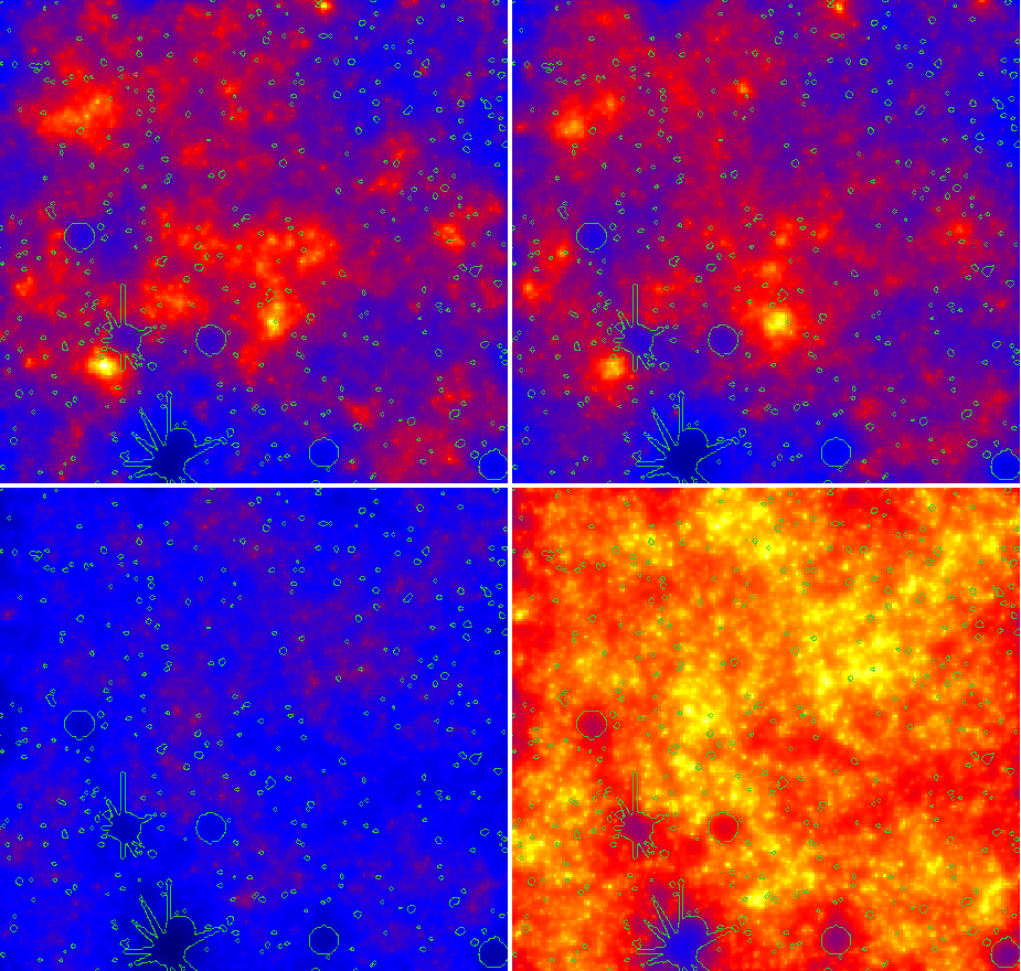
We show in the top left panel of Figure (9) the amplitude map for a slice at redshift resulting from the analysis of about 1 deg2 per side of the real KiDS data (top left panel). The green contour lines outline the areas masking the artefacts caused by bright stars and image defects in general. In the top right panel, we show the same analysis but performed on the corresponding mock catalogue of galaxies. All main features are clearly preserved and the small differences between the left and right maps are due both to the displacement of the galaxy positions, and to the Monte-Carlo sampling process. In practice, our mock map is a realization of the population of galaxies, statistically independent from the original. In the two bottom panels of the same figure, we plot with two different color scales the contribution to the amplitude of the mock field galaxies alone. The two top panels and bottom left one have the same color scale, while in the right bottom panel we stretched the contrast to better highlight the details such as the LSS pattern.
6.2 Uncertainties on the detections properties
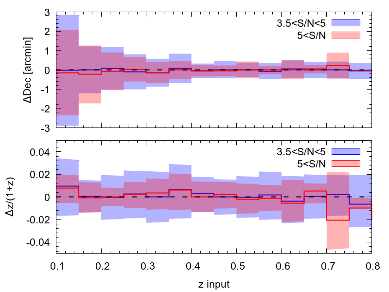
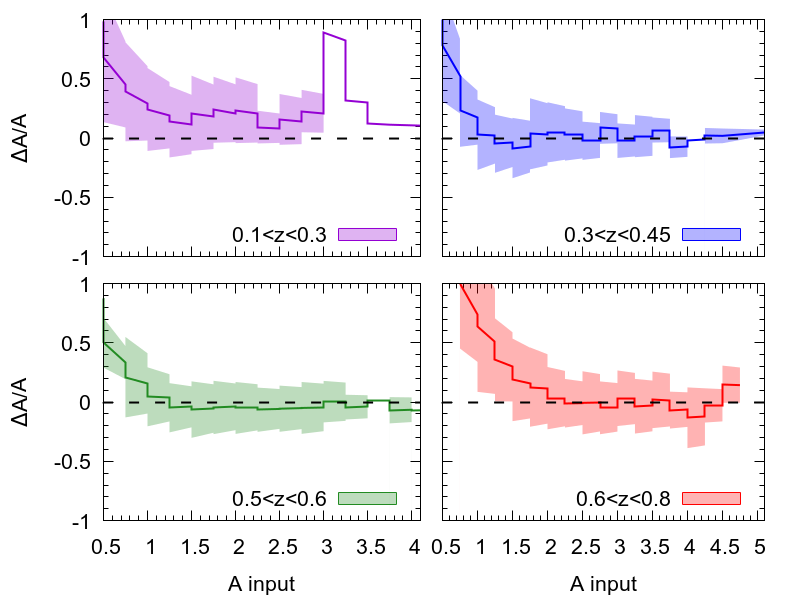
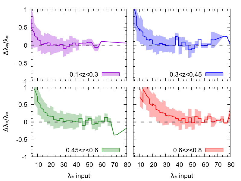
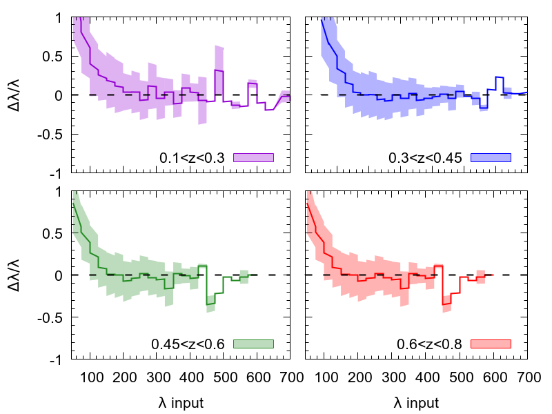
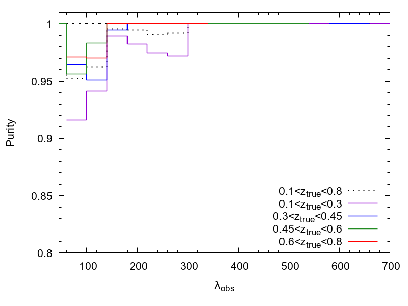
The uncertainties on the properties of the detections (position, redshift, amplitude, richness, etc…) are evaluated through the analysis of the mock catalogues by running on them the AMICO code as done with the real data and comparing the measured values with the expected ones. The errors (1 uncertainties) estimated in this way are listed in the final catalogue of detections. One detection is assigned to one mock cluster present in the simulations if they lay within a cylinder of in radius and of in length. The detections without a match are considered as spurious and allow us to derive the purity of the sample. The results are presented in Figure (10) and are discussed below.
Angular position: the scatter along the declination, , of the detections is larger for clusters at lower redshift because of their larger angular extension which does not allow for a well defined localization of their center. At higher redshift, , the angular resolution is dictated by the pixels size we have chosen for the maps produced by AMICO, that is of arcmin. The scatter along R.A. is completely analogous and because of this we do not shown it.
Redshift: the relative scatter in redshift is constant over the whole redshift interval and it amounts to , which is smaller then the one of the galaxy population (de Jong et al., 2017). The known bias of the galaxies photo- already discussed in de Jong et al. (2017) surely affects the redshift estimates of the detections but this does not show up in the top left panel of Figure (10). This is because the reference redshift of the mock clusters has been taken from the data and is therefore dragged by the very same bias. Nevertheless, this test serves to estimate the redshift uncertainty in a reliable way and shows that AMICO returns unbiased results with respect to the input photo- catalogue. We decided not to apply any correction to the redshifts of our sample to leave it as a separate step as more data against with to calibrate become available with time and the understanding of the photo- of the galaxies improves. The final redshift correction is thus left to the user but, based on the analysis discussed in Section (5.4), we suggest to apply the following relation to our sample in agreement with de Jong et al. (2017). Our approach differs from the one adopted in redMaPPer where such calibration against external spectroscopic data is done internally (Rykoff et al., 2014).
Amplitude: the relative scatter of the amplitude is almost constant over the whole range of values and in all four redshift intervals displayed in the top right four panels of Figure (10). At , the amplitude is biased down to a minimum value, which grows with redshift, below which the sample becomes incomplete and the Malmquist bias manifests itself as expected. In contrast, the amplitude of the lower redshift bin is biased high. We verified that this is not due to the masks which are more relevant for the lower redshift clusters because of their larger angular extension. The origin of this amplitude bias is not completely understood;
Richness: similar considerations hold for the intrinsic richness and apparent richness except for the fact that these quantities are unbiased at all redshifts.
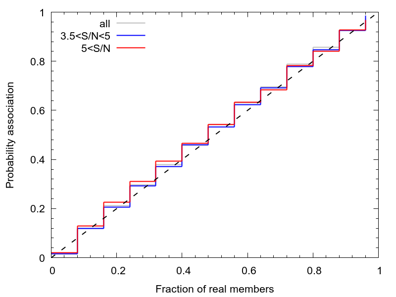
Membership probabilistic association: in Figure (11) we show the fraction of real members as a function of the measured probabilistic association of the galaxies to clusters (see Equation 4). Two different intervals of signal-to-noise ratio, that are and , are shown. The correlation well satisfies the identity proving that the association of galaxies to clusters is reliably estimated.
6.3 Purity and completeness
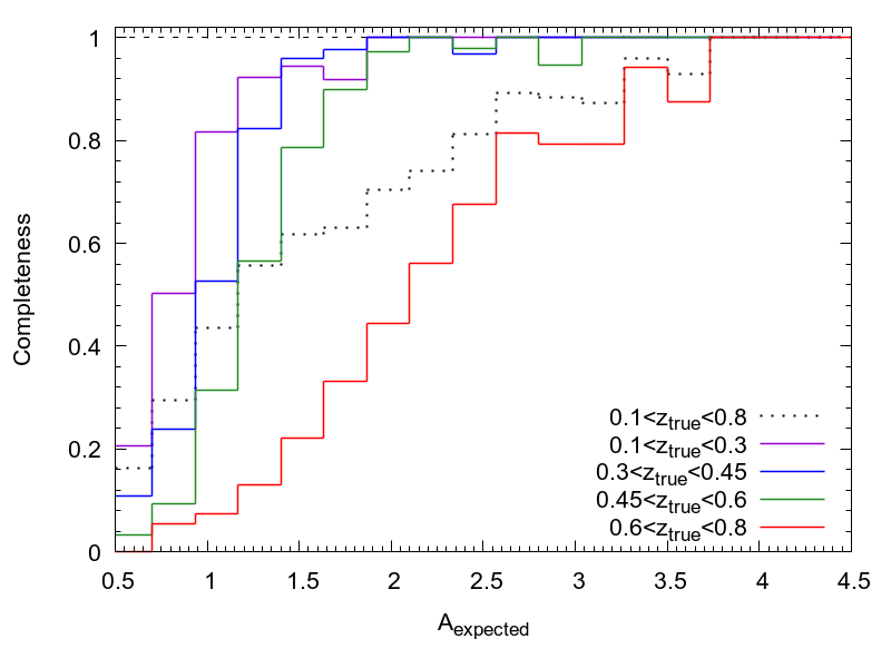
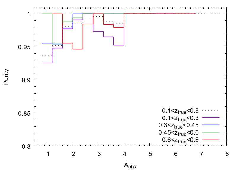
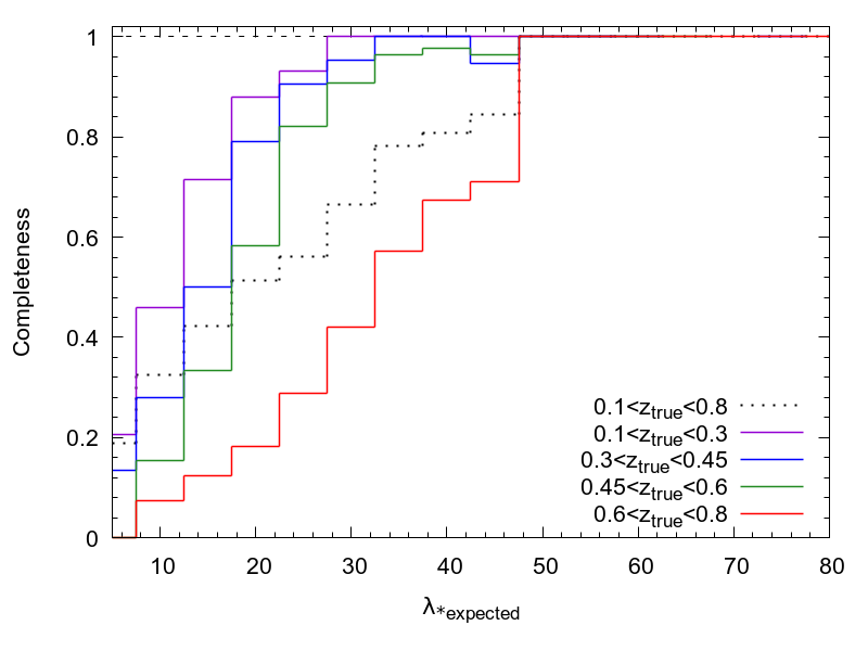
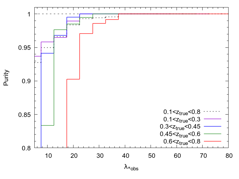
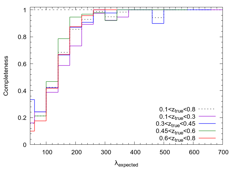
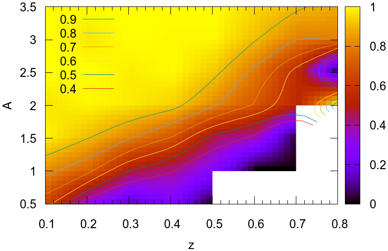
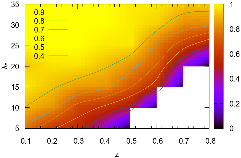
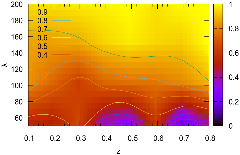
The completeness and the purity of the final sample are shown in Figure (12). The purity is a measure of the contamination level of the cluster sample and is defined as the fraction of detection successfully matched with the clusters in the simulations over the total number of detections. This is shown in the right panels of Figure (12). The sample purity is extremely high. The completeness, shown in the left panels, is defined as the fraction of detections with the fraction of mock clusters with a given amplitude or richness which have been detected correctly identified as clusters over the total number of mock clusters in the simulations. The minimum amplitude and intrinsic richness for which the sample is complete grows with redshift. This is because these two quantities are direct estimates of the clusters mass and, clearly, the larger is the redshift, the larger is the minimum mass for a cluster to be detected above a fixed minimum signal-to-noise ratio, that is in our case. This is not the case for the apparent richness, , because it quantifies the number of galaxies visible in a cluster that is mostly determined by the depth of the data. This missing or weak redshift dependence makes a better probe for cosmological studies. In Figure (13), we show the completeness as a function of redshift for different levels of amplitude , intrinsic richness , and apparent richness . Note that the completeness is measured not by setting a fixed mass threshold for all redshifts but instead it refers to a richness limit which on average grows with redshift. This definition is a consequence on how the mocks have been constructed. The population of clusters below such threshold is observationally un-accessible and could only be evaluated by assuming, for example, a mass function and a model relating dark matter haloes to visible galaxies, but such a study is not of our interest because fully model-dependent. What this method is aiming at is a model-independent selection function, related to completeness and purity, based on observables only that can then be used to investigate, for instance, the cosmological model or the star formation history. In fact, the mass proxies discussed in this paper can be related to actual masses for a direct comparison with theoretical models thanks to the scaling relations based on weak-lensing mass measurements derived in Bellagamba et al. submitted.
| NAME | unique identification name: AMICO-KIDS3-# |
|---|---|
| ID | unique identification number |
| FIELD | identification number ot the tile in which the detection has been found |
| XPIX, YPIX, ZPIX | the indexes of the pixel of the amplitude map in which the detection falls |
| XSKY, YSKY, ZSKY | sky coordinates R.A., Dec. and the redshift corresponding to XPIX, YPIX and ZPIX |
| A | amplitude, , as defined in Equation (6) |
| LAMBDA | apparent richness, , as defined in Equation (12) |
| LAMBDASTAR | intrinsic richness, , as defined in Equation (13) |
| XPIX_ERR, YPIX_ERR, ZPIX_ERR | 1 error of the position in pixel units |
| XSKY_ERR, YSKY_ERR, ZSKY_ERR | 1 error of the position in R.A., Dec. and the redshift |
| A_ERR | 1 error of the amplitude defined in Equation (2) |
| LAMBDA_ERR | 1 error of based on the mock catalogues |
| LAMBDASTAR_ERR | 1 error of based on the mock catalogues |
| SN | signal-to-noise ratio based on the amplitude, AMPLITUDE, and its r.m.s, A_ERR |
| LIKELIHOOD | likelihood derived in Equation (3) |
| MASKFRAC | fraction of the detection which is masked |
| ID_LITERATURE | identification number for those clusters already listed in the literature |
7 Conclusions
We detected galaxy clusters in the KiDS-DR3 data with the AMICO code. In the analysis, we avoided those regions of the sky affected by the presence of artefacts produced, for example, by bright stars and image artefacts, thus covering an effective area of deg2. With respect to our previous study of the KiDS-DR2 (Radovich et al., 2017), the work presented here takes advantage of the improvements with respect to the standard matched filter method introduced with the AMICO detection algorithm (Bellagamba et al., 2018), such as the cleaning procedure, a probability redshift distribution of the filter which now depends on the individual magnitude of the galaxies and a more robust approach to deal with possible biases in the galaxies photo-s. We detected galaxy clusters over a redshift range of with a minimum signal-to-noise ratio of . The catalog lists for each detection its unique identification number, sky position, redshift, amplitude , intrinsic richness , apparent richness , signa-to-noise ratio, likelihood , masked fraction, full probability redshift distribution and its name in the literature if present. In the process we also derived the probabilistic association of galaxies to each cluster, a useful information to study galaxy formation or help in the removal of the foreground for weak-lensing studies, just to mention some applications.
We compared our sample to public and private catalogues of galaxy clusters overlapping our fields, in particular: (1) we matched the cluster candidates detected by the redMaPPer algorithm on the Sloan Digital Sky Survey Data Release 8 (SDSS-DR8); (2) we detected all 19 Planck SZ-selected clusters present in our sky area and provide, for the first time, a redshift estimate for 10 of these objects; (3) we used the X-rays derived masses listed in the MCXC sample of clusters to test our mass proxies. Even if the set of common objects is not large enough to definitive conclusive results, the clear correlation we find is extremely encouraging; (4) finally, we used the GAMA-I galaxy group catalogue (G3C) to verify our redshift estimate. This allowed us to confirm the already known photo- bias affecting the KiDS data and derived the required calibration for its correction.
Finally, we proposed a new methodology based on the galaxy membership probabilistic association provided by AMICO to create realistic mock catalogues and use them to evaluate the uncertainties of all the properties of the detections, such as their angular position in the sky, redshift, and mass proxies. Most importantly, we use this method to derive the selection function of the sample in a fully model independent way. As it turned out, the sample has an extremely high purity, approaching % over the whole redshift range. This method provides the first step towards the measure of cosmological parameters through the use of photometrically selected galaxy clusters.
The catalogue of clusters and of the cluster members will be made publicly available but they can already be requested after submitting a proposal.
Appendix A Some example of detections
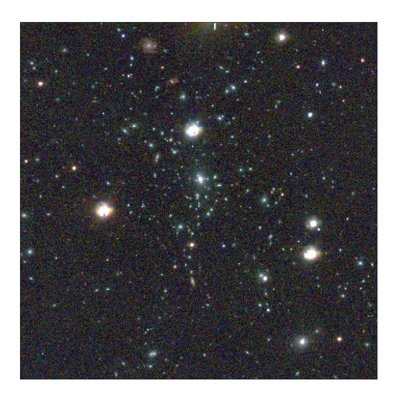
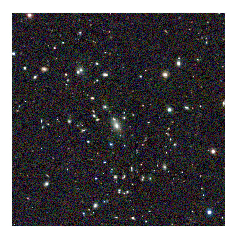
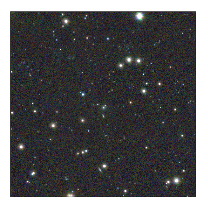
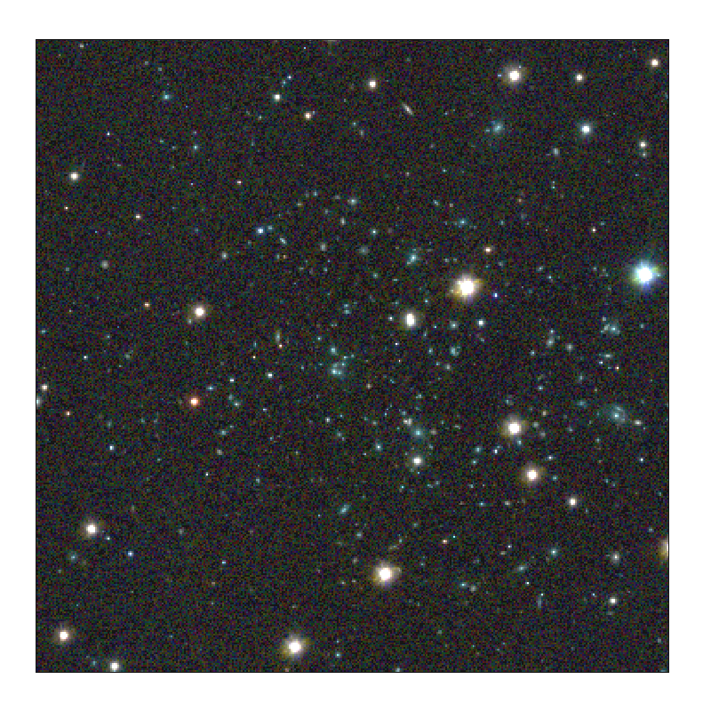
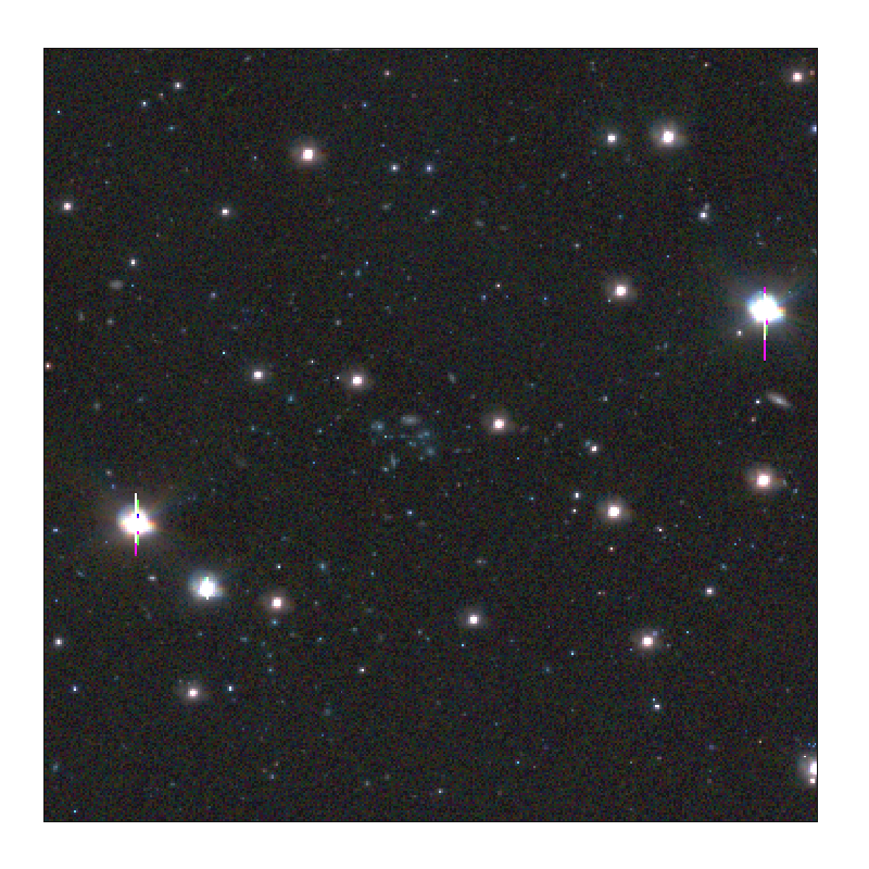
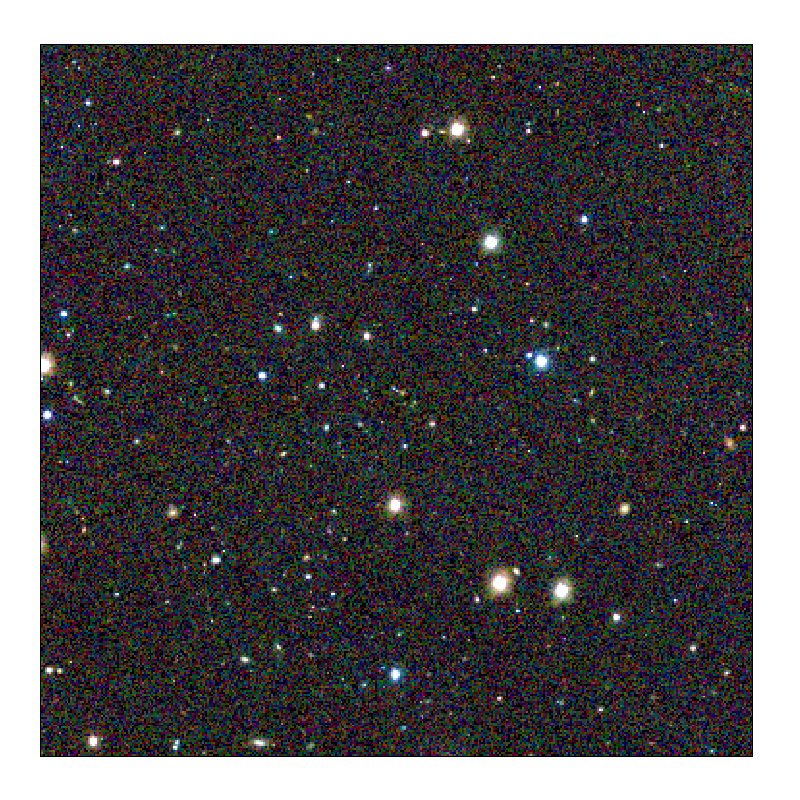
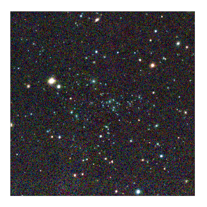
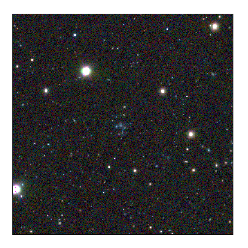
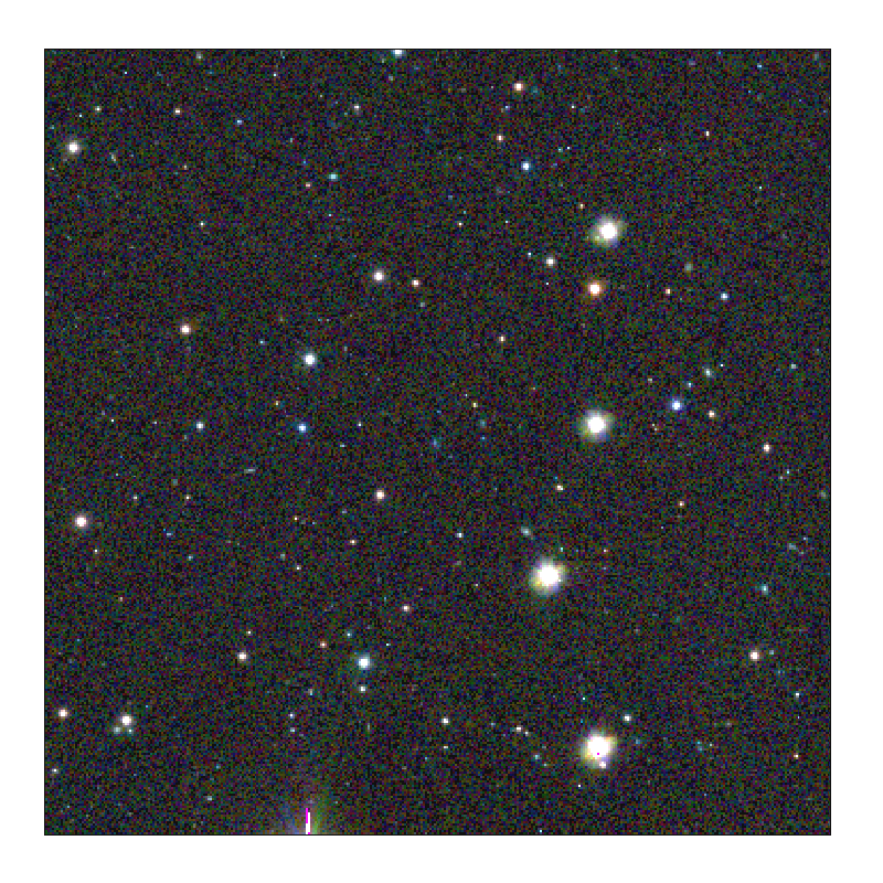
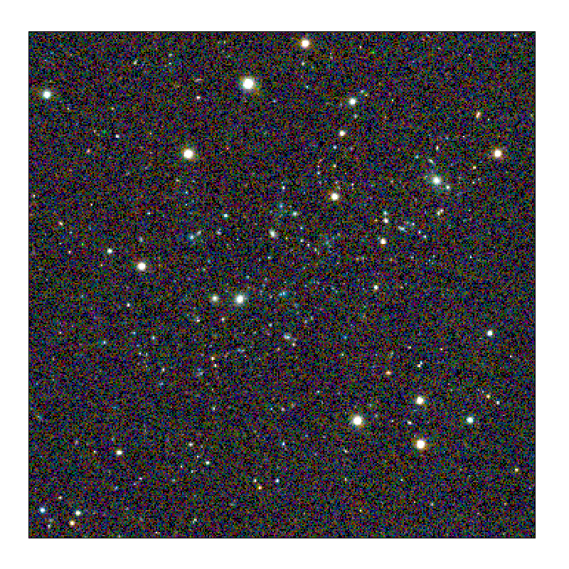
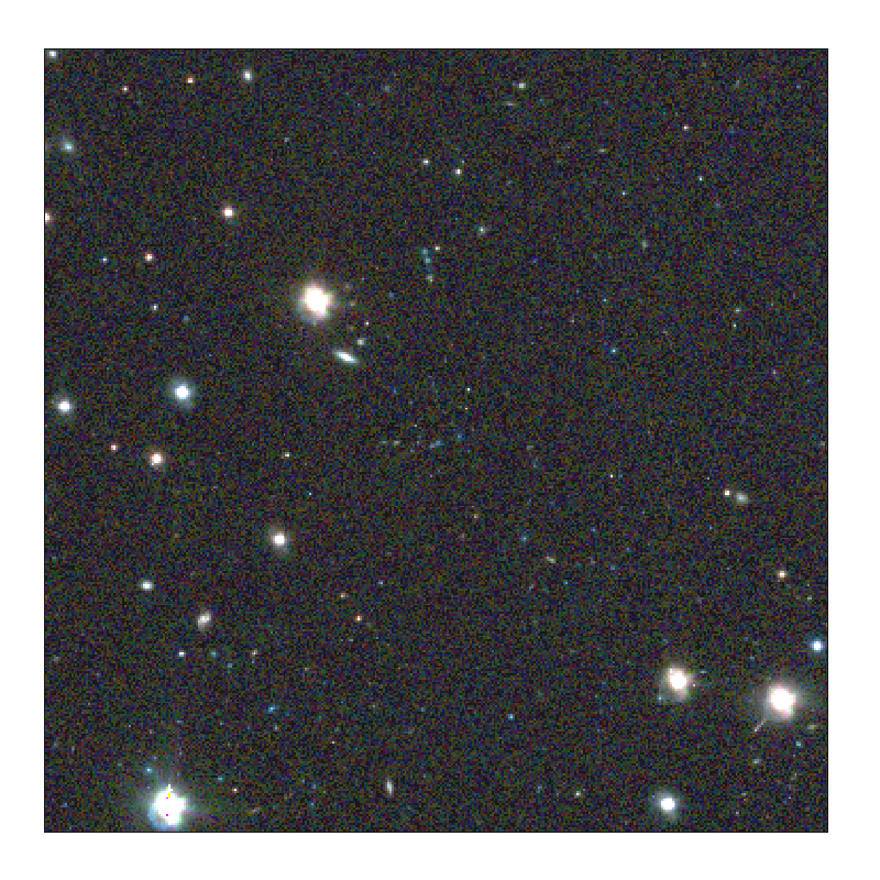
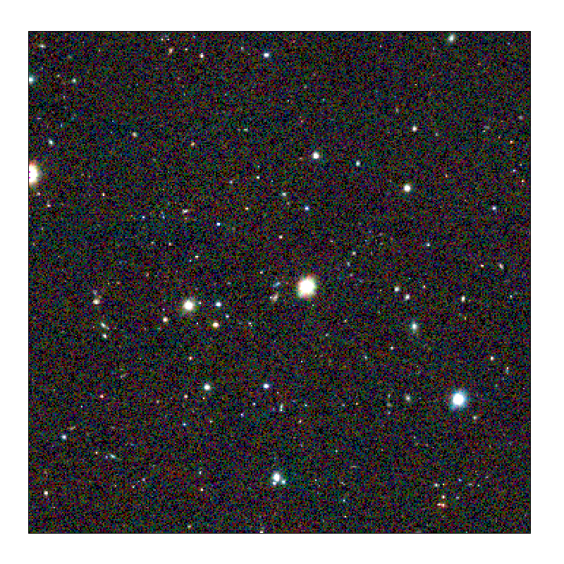
Here we show a sample of 12 detections located at four different redshifts (, , and , rows from top to bottom), and three different intrinsic richnesses (, and , column from left to right). All cut-outs are of arcsec in size.
Acknowledgements
This work was supported by the Collaborative Research Center TR33 ’The Dark Universe’. FB, MRo and LM thank the support from the grants ASI n.I/023/12/0 “Attivitá relative alla fase B2/C per la missione Euclid” and PRIN MIUR 2015 “Cosmology and Fundamental Physics: Illuminating the Dark Universe with Euclid”. MS acknowledges financial support from the contracts ASI-INAF I/009/10/0, NARO15 ASI-INAF I/037/12/0, ASI 2015-046-R.0, and ASI-INAF n.2017-14-H.0.
References
- Adami & Mazure (1999) Adami C., Mazure A., 1999, A&AS, 134, 393
- Amaro et al (2018) Amaro, V., Cavuoti S. ,Brescia M., Vallucci C. , Longo M., et al, 2018, MNRAS
- Bellagamba et al. (2011) Bellagamba F., Maturi M., Hamana T., Meneghetti M., Miyazaki S., Moscardini L., 2011, MNRAS, 413, 1145
- Bellagamba et al. (2018) Bellagamba F., Roncarelli M., Maturi M., Moscardini L., 2018, MNRAS, 473, 5221
- Benítez (2000) Benítez N., 2000, ApJ, 536, 571
- Benoist (2014) Benoist C., 2014, in Building the Euclid Cluster Survey - Scientific Program, proceedings of a conference held July 6-11 2014 at the Sexten Center for Astrophysics. Online at "http://www.sexten-cfa.eu/images/stories/conferenze2014/buildingclusters/Building_program_talks.pdf" id.8. p. 8
- Bilicki et al. (2018) Bilicki M., et al., 2018, A&A, 616, A69
- Böhringer et al. (2004) Böhringer H., et al., 2004, A&A, 425, 367
- Bradley et al. (2014) Bradley L. D., et al., 2014, ApJ, 792, 76
- Bruzual & Charlot (2003) Bruzual G., Charlot S., 2003, MNRAS, 344, 1000
- Capaccioli & Schipani (2011) Capaccioli M., Schipani P., 2011, The Messenger, 146, 2
- Carrasco et al. (2018) Carrasco M., Stapelberg S., Maturi M., Bartelmann M., Seidel G., Erben T., 2018, preprint, (arXiv:1807.03793)
- Clerc et al. (2014) Clerc N., et al., 2014, MNRAS, 444, 2723
- Coe et al. (2013) Coe D., et al., 2013, ApJ, 762, 32
- Corasaniti et al. (2018) Corasaniti P. S., Ettori S., Rasera Y., Sereno M., Amodeo S., Breton M.-A., Ghirardini V., Eckert D., 2018, ApJ, 862, 40
- Costanzi et al. (2013) Costanzi M., Villaescusa-Navarro F., Viel M., Xia J.-Q., Borgani S., Castorina E., Sefusatti E., 2013, J. Cosmology Astropart. Phys., 12, 012
- Driver et al. (2009) Driver S. P., et al., 2009, Astronomy and Geophysics, 50, 5.12
- Driver et al. (2011) Driver S. P., et al., 2011, MNRAS, 413, 971
- Farrens et al. (2011) Farrens S., Abdalla F. B., Cypriano E. S., Sabiu C., Blake C., 2011, MNRAS, 417, 1402
- Giocoli et al. (2018) Giocoli C., Moscardini L., Baldi M., Meneghetti M., Metcalf R. B., 2018, MNRAS, 478, 5436
- Gonzalez (2014) Gonzalez A., 2014, in Building the Euclid Cluster Survey - Scientific Program, proceedings of a conference held July 6-11 2014 at the Sexten Center for Astrophysics. Online at "http://www.sexten-cfa.eu/images/stories/conferenze2014/buildingclusters/Building_program_talks.pdf", id.7. p. 7
- Hennig et al. (2017) Hennig C., et al., 2017, MNRAS, 467, 4015
- Hilton et al. (2018) Hilton M., et al., 2018, ApJS, 235, 20
- Iovino (2014) Iovino A., 2014, in Building the Euclid Cluster Survey - Scientific Program, proceedings of a conference held July 6-11 2014 at the Sexten Center for Astrophysics. Online at "http://www.sexten-cfa.eu/images/stories/conferenze2014/buildingclusters/Building_program_talks.pdf", id.5. p. 5
- Kelly et al. (2015) Kelly P. L., et al., 2015, Science, 347, 1123
- Kuijken (2011) Kuijken K., 2011, The Messenger, 146, 8
- L’Huillier et al. (2017) L’Huillier B., Winther H. A., Mota D. F., Park C., Kim J., 2017, MNRAS, 468, 3174
- Licitra et al. (2016) Licitra R., Mei S., Raichoor A., Erben T., Hildebrandt H., 2016, MNRAS, 455, 3020
- Liske et al. (2015) Liske J., et al., 2015, MNRAS, 452, 2087
- Llinares & Mota (2013) Llinares C., Mota D. F., 2013, Physical Review Letters, 110, 151104
- Maturi et al. (2005) Maturi M., Meneghetti M., Bartelmann M., Dolag K., Moscardini L., 2005, A&A, 442, 851
- Maturi et al. (2007) Maturi M., Schirmer M., Meneghetti M., Bartelmann M., Moscardini L., 2007, A&A, 462, 473
- Merloni et al. (2012) Merloni A., et al., 2012, preprint, (arXiv:1209.3114)
- Navarro et al. (1997) Navarro J. F., Frenk C. S., White S. D. M., 1997, ApJ, 490, 493
- Pace et al. (2007) Pace F., Maturi M., Meneghetti M., Bartelmann M., Moscardini L., Dolag K., 2007, A&A, 471, 731
- Pace et al. (2008) Pace F., Maturi M., Bartelmann M., Cappelluti N., Dolag K., Meneghetti M., Moscardini L., 2008, A&A, 483, 389
- Padmanabhan et al. (2005) Padmanabhan N., et al., 2005, MNRAS, 359, 237
- Piffaretti et al. (2011) Piffaretti R., Arnaud M., Pratt G. W., Pointecouteau E., Melin J.-B., 2011, A&A, 534, A109
- Planck Collaboration et al. (2016a) Planck Collaboration et al., 2016a, A&A, 594, A13
- Planck Collaboration et al. (2016b) Planck Collaboration et al., 2016b, A&A, 594, A24
- Radovich et al. (2016) Radovich M., Puddu E., Bellagamba F., Moscardini L., Roncarelli M., Getman F., Grado A., 2016, The Universe of Digital Sky Surveys, 42, 189
- Radovich et al. (2017) Radovich M., et al., 2017, A&A, 598, A107
- Reichardt et al. (2013) Reichardt C. L., et al., 2013, ApJ, 763, 127
- Robotham et al. (2011) Robotham A. S. G., et al., 2011, MNRAS, 416, 2640
- Roncarelli et al. (2015) Roncarelli M., Carbone C., Moscardini L., 2015, MNRAS, 447, 1761
- Rydberg et al. (2018) Rydberg C.-E., Whalen D. J., Maturi M., Collett T., Carrasco M., Magg M., Klessen R. S., 2018, preprint, (arXiv:1805.02662)
- Rykoff et al. (2014) Rykoff E. S., et al., 2014, ApJ, 785, 104
- Sartoris et al. (2016) Sartoris B., et al., 2016, MNRAS, 459, 1764
- Schechter (1976) Schechter P., 1976, ApJ, 203, 297
- Schellenberger & Reiprich (2017) Schellenberger G., Reiprich T. H., 2017, MNRAS, 471, 1370
- Smith et al. (2016) Smith G. P., et al., 2016, MNRAS, 456, L74
- Stapelberg et al. (2017) Stapelberg S., Carrasco M., Maturi M., 2017, preprint, (arXiv:1709.09758)
- Umetsu et al. (2014) Umetsu K., et al., 2014, ApJ, 795, 163
- Viola et al. (2010) Viola M., Maturi M., Bartelmann M., 2010, MNRAS, 403, 859
- Wang et al. (2016) Wang B., Abdalla E., Atrio-Barandela F., Pavón D., 2016, Reports on Progress in Physics, 79, 096901
- Zenteno et al. (2016) Zenteno A., et al., 2016, MNRAS, 462, 830
- Zheng et al. (2012) Zheng W., et al., 2012, Nature, 489, 406
- de Haan et al. (2016) de Haan T., et al., 2016, ApJ, 832, 95
- de Jong et al. (2015) de Jong J. T. A., et al., 2015, A&A, 582, A62
- de Jong et al. (2017) de Jong J. T. A., et al., 2017, A&A, 604, A134