Doubly Semi-Implicit Variational Inference


Dmitry Molchanov1,2,∗                        Valery Kharitonov2,∗                        Artem Sobolev1                        Dmitry Vetrov1,2

dmolch111@gmail.com           kharvd@gmail.com           asobolev@bayesgroup.ru       vetrovd@yandex.ru 1 Samsung AI Center Moscow 2 Samsung-HSE Laboratory, National Research University Higher School of Economics Equal contribution

Abstract

We extend the existing framework of semi-implicit variational inference (SIVI) and introduce doubly semi-implicit variational inference (DSIVI), a way to perform variational inference and learning when both the approximate posterior and the prior distribution are semi-implicit. In other words, DSIVI performs inference in models where the prior and the posterior can be expressed as an intractable infinite mixture of some analytic density with a highly flexible implicit mixing distribution. We provide a sandwich bound on the evidence lower bound (ELBO) objective that can be made arbitrarily tight. Unlike discriminator-based and kernel-based approaches to implicit variational inference, DSIVI optimizes a proper lower bound on ELBO that is asymptotically exact. We evaluate DSIVI on a set of problems that benefit from implicit priors. In particular, we show that DSIVI gives rise to a simple modification of VampPrior, the current state-of-the-art prior for variational autoencoders, which improves its performance.

1 INTRODUCTION

Bayesian inference is an important tool in machine learning. It provides a principled way to reason about uncertainty in parameters or hidden representations. In recent years, there has been great progress in scalable Bayesian methods, which made it possible to perform approximate inference for large-scale datasets and deep learning models.

One of such methods is variational inference (VI) [3], which is an optimization-based approach. Given a probabilistic model p(x,z)=p(x|z)p(z)𝑝𝑥𝑧𝑝conditional𝑥𝑧𝑝𝑧p(x,z)=p(x\,|\,z)p(z), where x𝑥x are observed data and z𝑧z are latent variables, VI seeks to maximize the evidence lower bound (ELBO).

(ϕ)=𝔼qϕ(z)[logp(x|z)]KL(qϕ(z)p(z)),italic-ϕsubscript𝔼subscript𝑞italic-ϕ𝑧delimited-[]𝑝conditional𝑥𝑧KLconditionalsubscript𝑞italic-ϕ𝑧𝑝𝑧\mathcal{L}(\phi)=\mathbb{E}_{q_{\phi}(z)}[\log p(x\,|\,z)]-{\mathrm{KL}}(q_{\phi}(z)\,\|\,p(z)), (1)

where qϕ(z)subscript𝑞italic-ϕ𝑧q_{\phi}(z) approximates the intractable true posterior distribution p(z|x)𝑝conditional𝑧𝑥p(z\,|\,x). The parametric approximation family for qϕsubscript𝑞italic-ϕq_{\phi} is chosen in such a way, that we can efficiently estimate (ϕ)italic-ϕ\mathcal{L}(\phi) and its gradients w.r.t. ϕitalic-ϕ\phi.

Such approximations to the true posterior are often too simplistic. There exists a variety of ways to extend the variational family to mitigate this. They can be divided roughly into two main groups: those that require the probability density function of the approximate posterior to be analytically tractable (which we will call explicit models) [30, 12, 9, 5, 36, 38, 6, 27, 20] and those that do not (implicit models) [11, 22, 37, 17, 21, 31, 40]. For latter, we only assume that it is possible to sample from such distributions, whereas the density may be inaccessible.

Not only approximate posteriors but also priors in such models are often chosen to be very simple to make computations tractable. This can lead to overregularization and poor hidden representations in generative models such as variational autoencoders (VAE, [15]) [10, 35, 1]. In Bayesian neural networks, a standard normal prior is the default choice, but together with the mean field posterior, it can lead to overpruning and consequently underfitting [39]. To overcome such problem in practice, one usually scales the KL divergence term in the expression for ELBO or truncates the variances of the approximate posterior [24, 19, 18].

Another way to overcome this problem is to consider more complicated prior distributions, e.g. implicit priors. For example, hierarchical priors usually impose an implicit marginal prior when hyperparameters are integrated out. To perform inference in such models, one often resorts to joint inference over both parameters and hyperparameters, even though we are only interested in the marginal posterior over parameters of the model. Another example of implicit prior distributions is the optimal prior for variational autoencoders. It can be shown that the aggregated posterior distribution is the optimal prior for VAE [10], and it can be regarded as an implicit distribution. The VampPrior model [35] approximates this implicit prior using an explicit discrete mixture of Gaussian posteriors. However, this model can be further improved if we consider an arbitrary trainable semi-implicit prior.

In this paper, we extend the recently proposed framework of semi-implicit variational inference (SIVI) [40] and consider priors and posteriors that are defined as semi-implicit distributions. By “semi-implicit” we mean distributions that do not have a tractable PDF (i.e. implicit), but that can be represented as a mixture of some analytically tractable density with a flexible mixing distribution, either explicit or implicit.

Our contributions can be summarized as follows. Firstly, we prove that the SIVI objective is actually a lower bound on the true ELBO, which allows us to sandwich the ELBO between an upper bound and a lower bound which are both asymptotically exact. Secondly, we propose doubly semi-implicit variational inference (DSIVI), a general-purpose framework for variational inference and variational learning in the case when both the posterior and the prior are semi-implicit. We construct a SIVI-inspired asymptotically exact lower bound on the ELBO for this case, and use the variational representation of the KL divergence to obtain the upper bound. Finally, we consider a wide range of applications where semi-implicit distributions naturally arise, and show how the use of DSIVI in these settings is beneficial.

2 PRELIMINARIES

Consider a probabilistic model defined by its joint distribution p(x,z)=p(x|z)p(z)𝑝𝑥𝑧𝑝conditional𝑥𝑧𝑝𝑧p(x,z)=p(x\,|\,z)p(z), where variables x𝑥x are observed, and z𝑧z are the latent variables. Variational inference is a family of methods that approximate the intractable posterior distribution p(z|x)𝑝conditional𝑧𝑥p(z\,|\,x) with a tractable parametric distribution qϕ(z)subscript𝑞italic-ϕ𝑧q_{\phi}(z). To do so, VI methods maximize the evidence lower bound (ELBO):

logp(x)(ϕ)=𝔼qϕ(z)logp(x|z)p(z)qϕ(z)maxϕ.𝑝𝑥italic-ϕsubscript𝔼subscript𝑞italic-ϕ𝑧𝑝conditional𝑥𝑧𝑝𝑧subscript𝑞italic-ϕ𝑧subscriptitalic-ϕ\log p(x)\geq\mathcal{L}(\phi)=\mathbb{E}_{q_{\phi}(z)}\log\frac{p(x\,|\,z)p(z)}{q_{\phi}(z)}\to\max_{\phi}. (2)

The maximum of the evidence lower bound corresponds to the minimum of the KL-divergence KL(qϕ(z)p(z|x)){\mathrm{KL}}(q_{\phi}(z)\,\|\,p(z\,|\,x)) between the variational distribution qϕ(z)subscript𝑞italic-ϕ𝑧q_{\phi}(z) and the exact posterior p(z|x)𝑝conditional𝑧𝑥p(z\,|\,x). In the more general variational learning setting, the prior distribution may also be a parametric distribution pθ(z)subscript𝑝𝜃𝑧p_{\theta}(z) [11]. In this case, one would optimize the ELBO w.r.t. both the variational parameters ϕitalic-ϕ\phi and the prior parameters θ𝜃\theta, thus performing approximate maximization of the marginal likelihood p(x|θ)𝑝conditional𝑥𝜃p(x\,|\,\theta).

The common way to estimate the gradient of this objective is to use the reparameterization trick [15]. The reparameterization trick recasts the sampling from the parametric distribution qϕ(z)subscript𝑞italic-ϕ𝑧q_{\phi}(z) as the sampling of non-parametric noise εp(ε)similar-to𝜀𝑝𝜀\varepsilon\sim p(\varepsilon), followed by a deterministic parametric transformation z=f(ε,ϕ)𝑧𝑓𝜀italic-ϕz=f(\varepsilon,\phi). Still, such gradient estimator requires log-densities of both the prior distribution p(z)𝑝𝑧p(z) and the approximate posterior qϕ(z)subscript𝑞italic-ϕ𝑧q_{\phi}(z) in closed form. Several methods have been proposed to overcome this limitation [27, 21, 31]. However, such methods usually provide a biased estimate of the evidence lower bound with no practical way of estimating the introduced bias.

The reparameterizable distributions with no closed-form densities are usually referred to as implicit distributions. In this paper we consider the so-called semi-implicit distributions that are defined as an implicit mixture of explicit conditional distributions:

qϕ(z)=qϕ(z|ψ)qϕ(ψ)𝑑ψ.subscript𝑞italic-ϕ𝑧subscript𝑞italic-ϕconditional𝑧𝜓subscript𝑞italic-ϕ𝜓differential-d𝜓q_{\phi}(z)=\int q_{\phi}(z\,|\,\psi)q_{\phi}(\psi)\,d\psi. (3)

Here, the conditional distribution qϕ(z|ψ)subscript𝑞italic-ϕconditional𝑧𝜓q_{\phi}(z\,|\,\psi) is explicit. However, when its condition ψ𝜓\psi follows an implicit distribution qϕ(ψ)subscript𝑞italic-ϕ𝜓q_{\phi}(\psi), the resulting marginal distribution qϕ(z)subscript𝑞italic-ϕ𝑧q_{\phi}(z) is implicit. We will refer to qϕ(ψ)subscript𝑞italic-ϕ𝜓q_{\phi}(\psi) as the mixing distribution, and to ψ𝜓\psi as the mixing variables.

Note that we may easily sample from semi-implicit distributions: in order to sample z𝑧z from qϕ(z)subscript𝑞italic-ϕ𝑧q_{\phi}(z), we need to first sample the mixing variable ψqϕ(ψ)similar-to𝜓subscript𝑞italic-ϕ𝜓\psi\sim q_{\phi}(\psi), and then sample z𝑧z from the conditional qϕ(z|ψ)subscript𝑞italic-ϕconditional𝑧𝜓q_{\phi}(z\,|\,\psi). Further in the text, we will assume this sampling scheme when using expectations 𝔼zqϕ(z)subscript𝔼similar-to𝑧subscript𝑞italic-ϕ𝑧\mathbb{E}_{z\sim q_{\phi}(z)} over semi-implicit distributions. Also note that an arbitrary implicit distribution can be represented in a semi-implicit form: qϕ(z)=δ(zz)qϕ(z)𝑑zsubscript𝑞italic-ϕ𝑧𝛿𝑧superscript𝑧subscript𝑞italic-ϕsuperscript𝑧differential-dsuperscript𝑧q_{\phi}(z)=\int\delta(z-z^{\prime})q_{\phi}(z^{\prime})\,dz^{\prime}.

3 RELATED WORK

There are several approaches to inference and learning in models with implicit distributions.

One approach is commonly referred to as hierarchical variational inference or auxiliary variable models. It allows for inference with implicit approximate posteriors qϕ(z)subscript𝑞italic-ϕ𝑧q_{\phi}(z) that can be represented as a marginal distribution of an explicit joint distribution qϕ(z)=qϕ(z,ψ)𝑑ψsubscript𝑞italic-ϕ𝑧subscript𝑞italic-ϕ𝑧𝜓differential-d𝜓q_{\phi}(z)=\int q_{\phi}(z,\psi)\,d\psi. The ELBO is then bounded from below using a reverse variational model rω(ψ|z)qϕ(ψ|z)subscript𝑟𝜔conditional𝜓𝑧subscript𝑞italic-ϕconditional𝜓𝑧r_{\omega}(\psi\,|\,z)\approx q_{\phi}(\psi\,|\,z) [27, 29, 19]. This method does not allow for implicit prior distributions, requires access to the explicit joint density qϕ(z,ψ)subscript𝑞italic-ϕ𝑧𝜓q_{\phi}(z,\psi) and has no way to estimate the increased inference gap, introduced by the imperfect reverse model. However, recently proposed deep weight prior [2] provides a new lower bound, suitable for learning hierarchical priors in a similar fashion.

Another family of models uses an optimal discriminator to estimate the ratio of implicit densities r(z)=qϕ(z)pθ(z)𝑟𝑧subscript𝑞italic-ϕ𝑧subscript𝑝𝜃𝑧r(z)=\frac{q_{\phi}(z)}{p_{\theta}(z)} [21, 22, 11]. This is the most general approach to inference and learning with implicit distributions, but it also optimizes a biased surrogate ELBO, and the induced bias cannot be estimated. Also, different authors report that the performance of this approach is poor if the dimensionality of the implicit densities is high [32, 37]. This is the only approach that allows to perform variational learning (learning the parameters θ𝜃\theta of the prior distribution pθ(z)subscript𝑝𝜃𝑧p_{\theta}(z)). However, it is non-trivial and requires differentiation through a series of SGD updates. This approach has not been validated in practice yet and has only been proposed as a theoretical concept [11]. On the contrary, DSIVI provides a lower bound that can be directly optimized w.r.t. both the variational parameters ϕitalic-ϕ\phi and the prior parameters θ𝜃\theta, naturally enabling variational learning.

Kernel implicit variational inference (KIVI) [31] is another approach that uses kernelized ridge regression to approximate the density ratio. It is reported to be more stable than the discriminator-based approaches, as the proposed density ratio estimator can be computed in closed form. Still, this procedure introduces a bias that is not addressed. Also, KIVI relies on adaptive contrast that does not allow for implicit prior distributions [21, 31].

There are also alternative formulations of variational inference that are based on different divergences. One example is operator variational inference [26] that uses the Langevin-Stein operator to design a new variational objective. Although it allows for arbitrary implicit posterior approximations, the prior distribution has to be explicit.

4 DOUBLY SEMI-IMPLICIT VARIATIONAL INFERENCE

In this section, we will describe semi-implicit variational inference, study its properties, and then extend it for the case of semi-implicit prior distributions.

4.1 Semi-Implicit Variational Inference

Semi-implicit variational inference [40] considers models with an explicit joint distribution p(x,z)𝑝𝑥𝑧p(x,z) and a semi-implicit approximate posterior qϕ(z)subscript𝑞italic-ϕ𝑧q_{\phi}(z), as defined in Eq. (3). The basic idea of semi-implicit variational inference is to approximate the semi-implicit approximate posterior with a finite mixture:

qϕ(z)subscript𝑞italic-ϕ𝑧\displaystyle q_{\phi}(z) =qϕ(z|ψ)qϕ(ψ)𝑑ψabsentsubscript𝑞italic-ϕconditional𝑧𝜓subscript𝑞italic-ϕ𝜓differential-d𝜓absent\displaystyle=\int q_{\phi}(z\,|\,\psi)q_{\phi}(\psi)\,d\psi\approx (4)
1Kk=1Kqϕ(z|ψk),ψkqϕ(ψ).formulae-sequenceabsent1𝐾superscriptsubscript𝑘1𝐾subscript𝑞italic-ϕconditional𝑧superscript𝜓𝑘similar-tosuperscript𝜓𝑘subscript𝑞italic-ϕ𝜓\displaystyle\approx\frac{1}{K}\sum_{k=1}^{K}q_{\phi}(z\,|\,\psi^{k}),\ \ \ \psi^{k}\sim q_{\phi}(\psi).

SIVI provides an upper bound ¯Kq¯K+1qsubscriptsuperscript¯𝑞𝐾subscriptsuperscript¯𝑞𝐾1\overline{\mathcal{L}}^{q}_{K}\geq\overline{\mathcal{L}}^{q}_{K+1}\geq\mathcal{L}, and a surrogate objective ¯Kqsubscriptsuperscript¯𝑞𝐾\underline{\mathcal{L}}^{q}_{K} that both converge to ELBO as K𝐾K goes to infinity (¯q=¯q=subscriptsuperscript¯𝑞subscriptsuperscript¯𝑞\underline{\mathcal{L}}^{q}_{\infty}=\overline{\mathcal{L}}^{q}_{\infty}=\mathcal{L}):

¯Kq=𝔼qϕ(z)logp(x|z)p(z)subscriptsuperscript¯𝑞𝐾limit-fromsubscript𝔼subscript𝑞italic-ϕ𝑧𝑝conditional𝑥𝑧𝑝𝑧\displaystyle\overline{\mathcal{L}}^{q}_{K}=\mathbb{E}_{q_{\phi}(z)}\log{p(x\,|\,z)p(z)}- (5)
𝔼ψ0..Kqϕ(ψ)𝔼zqϕ(z|ψ0)log1Kk=1Kqϕ(z|ψk),\displaystyle-\mathbb{E}_{\psi^{0..K}\sim q_{\phi}(\psi)}\mathbb{E}_{z\sim q_{\phi}(z\,|\,\psi^{0})}\log{\frac{1}{K}\sum_{k=1}^{K}q_{\phi}(z\,|\,\psi^{k})},
¯Kq=𝔼qϕ(z)logp(x|z)p(z)subscriptsuperscript¯𝑞𝐾limit-fromsubscript𝔼subscript𝑞italic-ϕ𝑧𝑝conditional𝑥𝑧𝑝𝑧\displaystyle\underline{\mathcal{L}}^{q}_{K}=\mathbb{E}_{q_{\phi}(z)}\log{p(x\,|\,z)p(z)}- (6)
𝔼ψ0..Kqϕ(ψ)𝔼zqϕ(z|ψ0)log1K+1k=0Kqϕ(z|ψk).\displaystyle-\mathbb{E}_{\psi^{0..K}\sim q_{\phi}(\psi)}\mathbb{E}_{z\sim q_{\phi}(z\,|\,\psi^{0})}\log{\frac{1}{K+1}\sum_{k=0}^{K}q_{\phi}(z\,|\,\psi^{k})}.

The surrogate objective ¯Kqsubscriptsuperscript¯𝑞𝐾\underline{\mathcal{L}}^{q}_{K} is then used for optimization.

4.2 SIVI Lower Bound

Although it was shown that ¯0qsubscriptsuperscript¯𝑞0\underline{\mathcal{L}}^{q}_{0} is a lower bound for ELBO, it has not been clear whether this holds for arbitrary K𝐾K, and whether maximizing ¯Kqsubscriptsuperscript¯𝑞𝐾\underline{\mathcal{L}}^{q}_{K} leads to a correct procedure. Here, we show that ¯Kqsubscriptsuperscript¯𝑞𝐾\underline{\mathcal{L}}^{q}_{K} is indeed a lower bound on ELBO \mathcal{L}.

Theorem 1.

Consider \mathcal{L} and ¯Kqsubscriptsuperscript¯𝑞𝐾\underline{\mathcal{L}}^{q}_{K} defined as in Eq. (2) and (6). Then ¯Kqsubscriptsuperscript¯𝑞𝐾\underline{\mathcal{L}}^{q}_{K} converges to \mathcal{L} from below as K𝐾K\to\infty, satisfying ¯Kq¯K+1qsubscriptsuperscript¯𝑞𝐾subscriptsuperscript¯𝑞𝐾1\underline{\mathcal{L}}^{q}_{K}\leq\underline{\mathcal{L}}^{q}_{K+1}\leq\mathcal{L}, and

¯Kq=𝔼ψ0..Kqϕ(ψ)𝔼qϕK(z|ψ0..K)logp(x|z)p(z)qϕK(z|ψ0..K),\displaystyle\underline{\mathcal{L}}^{q}_{K}=\mathbb{E}_{\psi^{0..K}\sim q_{\phi}(\psi)}\mathbb{E}_{q_{\phi}^{K}(z\,|\,\psi^{0..K})}\log{\frac{p(x\,|\,z)p(z)}{q_{\phi}^{K}(z\,|\,\psi^{0..K})}}, (7)
where qϕK(z|ψ0..K)=1K+1k=0Kqϕ(z|ψk).\displaystyle\text{where }q_{\phi}^{K}(z\,|\,\psi^{0..K})=\frac{1}{K+1}\sum_{k=0}^{K}q_{\phi}(z\,|\,\psi^{k}). (8)

The proof can be found in Appendix A.

It can be seen from Eq. (7) that the surrogate objective ¯Kqsubscriptsuperscript¯𝑞𝐾\underline{\mathcal{L}}^{q}_{K} proposed by [40] is actually the ELBO for a finite mixture approximation qϕK(z|ψ0,,ψK)superscriptsubscript𝑞italic-ϕ𝐾conditional𝑧superscript𝜓0superscript𝜓𝐾q_{\phi}^{K}(z\,|\,\psi^{0},\dots,\psi^{K}), that is averaged over all such mixtures (averaged over samples of ψ0,,ψKqϕ(ψ)similar-tosuperscript𝜓0superscript𝜓𝐾subscript𝑞italic-ϕ𝜓\psi^{0},\dots,\psi^{K}\sim q_{\phi}(\psi)).

4.3 Semi-Implicit Priors

Inspired by the derivation of the SIVI upper bound, we can derive the lower bound ¯Kpsubscriptsuperscript¯𝑝𝐾\underline{\mathcal{L}}^{p}_{K} for the case of semi-implicit prior distributions. Right now, for simplicity, assume an explicit approximate posterior qϕ(z)subscript𝑞italic-ϕ𝑧q_{\phi}(z), and a semi-implicit prior pθ(z)=pθ(z|ζ)pθ(ζ)𝑑ζsubscript𝑝𝜃𝑧subscript𝑝𝜃conditional𝑧𝜁subscript𝑝𝜃𝜁differential-d𝜁p_{\theta}(z)=\int p_{\theta}(z|\zeta)p_{\theta}(\zeta)\,d\zeta

¯Kp=𝔼qϕ(z)logp(x|z)𝔼ζ1..Kpθ(ζ)𝔼qϕ(z)logqϕ(z)1Kk=1Kpθ(z|ζk),\displaystyle\begin{multlined}\underline{\mathcal{L}}^{p}_{K}=\mathbb{E}_{q_{\phi}(z)}\log{p(x\,|\,z)}-\\ -\mathbb{E}_{\zeta^{1..K}\sim p_{\theta}(\zeta)}\mathbb{E}_{q_{\phi}(z)}\log\frac{q_{\phi}(z)}{\frac{1}{K}\sum_{k=1}^{K}p_{\theta}(z\,|\,\zeta^{k})},\end{multlined}\underline{\mathcal{L}}^{p}_{K}=\mathbb{E}_{q_{\phi}(z)}\log{p(x\,|\,z)}-\\ -\mathbb{E}_{\zeta^{1..K}\sim p_{\theta}(\zeta)}\mathbb{E}_{q_{\phi}(z)}\log\frac{q_{\phi}(z)}{\frac{1}{K}\sum_{k=1}^{K}p_{\theta}(z\,|\,\zeta^{k})}, (11)
¯Kp¯K+1p¯p=.subscriptsuperscript¯𝑝𝐾subscriptsuperscript¯𝑝𝐾1subscriptsuperscript¯𝑝\displaystyle\underline{\mathcal{L}}^{p}_{K}\leq\underline{\mathcal{L}}^{p}_{K+1}\leq\underline{\mathcal{L}}^{p}_{\infty}=\mathcal{L}. (12)

This bound has the same properties: it is non-decreasing in K𝐾K and is asymptotically exact. To see why ¯Kpsubscriptsuperscript¯𝑝𝐾\underline{\mathcal{L}}^{p}_{K}\leq\mathcal{L}, one just needs to apply the Jensen’s inequality for the logarithm:

𝔼ζ1..Kpθ(ζ)𝔼qϕ(z)log1Kk=1Kpθ(z|ζk)𝔼qϕ(z)log𝔼ζ1..Kpθ(ζ)1Kk=1Kpθ(z|ζk)==𝔼qϕ(z)logpθ(z).\begin{multlined}\mathbb{E}_{\zeta^{1..K}\sim p_{\theta}(\zeta)}\mathbb{E}_{q_{\phi}(z)}\log{\frac{1}{K}\sum_{k=1}^{K}p_{\theta}(z\,|\,\zeta^{k})}\leq\\[-5.0pt] \begin{aligned} &\leq\mathbb{E}_{q_{\phi}(z)}\log{\mathbb{E}_{\zeta^{1..K}\sim p_{\theta}(\zeta)}\frac{1}{K}\sum_{k=1}^{K}p_{\theta}(z\,|\,\zeta^{k})}=\\ &=\mathbb{E}_{q_{\phi}(z)}\log{p_{\theta}(z)}.\end{aligned}\end{multlined}\mathbb{E}_{\zeta^{1..K}\sim p_{\theta}(\zeta)}\mathbb{E}_{q_{\phi}(z)}\log{\frac{1}{K}\sum_{k=1}^{K}p_{\theta}(z\,|\,\zeta^{k})}\leq\\[-5.0pt] \begin{aligned} &\leq\mathbb{E}_{q_{\phi}(z)}\log{\mathbb{E}_{\zeta^{1..K}\sim p_{\theta}(\zeta)}\frac{1}{K}\sum_{k=1}^{K}p_{\theta}(z\,|\,\zeta^{k})}=\\ &=\mathbb{E}_{q_{\phi}(z)}\log{p_{\theta}(z)}.\end{aligned} (13)

To show that this bound is non-decreasing in K𝐾K, one can refer to the proof of proposition 3 in the SIVI paper [40, Appendix A].

Note that it is no longer possible to use the same trick to obtain the upper bound. Still, we can obtain an upper bound using the variational representation of the KL-divergence [25]:

KL(qϕ(z)pθ(z))==1+supg:domz{𝔼qϕ(z)g(z)𝔼pθ(z)eg(z)}1+supη{𝔼qϕ(z)g(z,η)𝔼pθ(z)eg(z,η)},KLconditionalsubscript𝑞italic-ϕ𝑧subscript𝑝𝜃𝑧1subscriptsupremum:𝑔dom𝑧subscript𝔼subscript𝑞italic-ϕ𝑧𝑔𝑧subscript𝔼subscript𝑝𝜃𝑧superscript𝑒𝑔𝑧1subscriptsupremum𝜂subscript𝔼subscript𝑞italic-ϕ𝑧𝑔𝑧𝜂subscript𝔼subscript𝑝𝜃𝑧superscript𝑒𝑔𝑧𝜂\displaystyle\begin{multlined}{\mathrm{KL}}(q_{\phi}(z)\,\|\,p_{\theta}(z))=\\ =1+\sup_{g:\mathrm{dom}\,z\to\mathbb{R}}\left\{\mathbb{E}_{q_{\phi}(z)}g(z)-\mathbb{E}_{p_{\theta}(z)}e^{g(z)}\right\}\geq\\ \geq 1+\sup_{\eta}\left\{\mathbb{E}_{q_{\phi}(z)}g(z,\eta)-\mathbb{E}_{p_{\theta}(z)}e^{g(z,\eta)}\right\},\end{multlined}{\mathrm{KL}}(q_{\phi}(z)\,\|\,p_{\theta}(z))=\\ =1+\sup_{g:\mathrm{dom}\,z\to\mathbb{R}}\left\{\mathbb{E}_{q_{\phi}(z)}g(z)-\mathbb{E}_{p_{\theta}(z)}e^{g(z)}\right\}\geq\\ \geq 1+\sup_{\eta}\left\{\mathbb{E}_{q_{\phi}(z)}g(z,\eta)-\mathbb{E}_{p_{\theta}(z)}e^{g(z,\eta)}\right\}, (17)
¯ηp=𝔼qϕ(z)logp(x|z)1𝔼qϕ(z)g(z,η)+𝔼pθ(z)eg(z,η).subscriptsuperscript¯𝑝𝜂subscript𝔼subscript𝑞italic-ϕ𝑧𝑝conditional𝑥𝑧1subscript𝔼subscript𝑞italic-ϕ𝑧𝑔𝑧𝜂subscript𝔼subscript𝑝𝜃𝑧superscript𝑒𝑔𝑧𝜂\displaystyle\begin{multlined}\overline{\mathcal{L}}^{p}_{\eta}=\mathbb{E}_{q_{\phi}(z)}\log{p(x\,|\,z)}-\\ -1-\mathbb{E}_{q_{\phi}(z)}g(z,\eta)+\mathbb{E}_{p_{\theta}(z)}e^{g(z,\eta)}.\end{multlined}\overline{\mathcal{L}}^{p}_{\eta}=\mathbb{E}_{q_{\phi}(z)}\log{p(x\,|\,z)}-\\ -1-\mathbb{E}_{q_{\phi}(z)}g(z,\eta)+\mathbb{E}_{p_{\theta}(z)}e^{g(z,\eta)}. (20)

Here we substitute the maximization over all functions with a single parametric function. In order to obtain a tighter bound, we can minimize this bound w.r.t. the parameters η𝜂\eta of function g(z,η)𝑔𝑧𝜂g(z,\eta).

Note that in order to find the optimal value for η𝜂\eta, one does not need to estimate the entropy term or the likelihood term of the objective:

η=argminη[𝔼qϕ(z)g(z,η)+𝔼pθ(z)eg(z,η)].superscript𝜂subscript𝜂subscript𝔼subscript𝑞italic-ϕ𝑧𝑔𝑧𝜂subscript𝔼subscript𝑝𝜃𝑧superscript𝑒𝑔𝑧𝜂\eta^{*}=\arg\min_{\eta}\left[-\mathbb{E}_{q_{\phi}(z)}g(z,\eta)+\mathbb{E}_{p_{\theta}(z)}e^{g(z,\eta)}\right]. (21)

This allows us to obtain a lower bound on the KL-divergence between two arbitrary (semi-)implicit distributions, and, consequently, results in an upper bound on the ELBO.

4.4 Final Objective

We can combine the bounds for the semi-implicit posterior and the semi-implicit prior to obtain the final lower bound

¯¯K1,K2q,p=𝔼qϕ(z)logp(x|z)𝔼ψ0..K1qϕ(ψ)𝔼qϕ(z|ψ0)log1K1+1k=0K1qϕ(z|ψk)+\begin{split}&\underline{\underline{\mathcal{L}}}_{K_{1},K_{2}}^{q,p}=\mathbb{E}_{q_{\phi}(z)}\log{p(x\,|\,z)}-\\ &-\mathbb{E}_{\psi^{0..K_{1}}\sim q_{\phi}(\psi)}\mathbb{E}_{q_{\phi}(z\,|\,\psi^{0})}\log\frac{1}{K_{1}+1}\sum_{k=0}^{K_{1}}q_{\phi}(z\,|\,\psi^{k})+\\ \end{split}
+𝔼ζ1..K2pθ(ζ)𝔼qϕ(z)log1K2k=1K2pθ(z|ζk),\begin{split}&+\mathbb{E}_{\zeta^{1..K_{2}}\sim p_{\theta}(\zeta)}\mathbb{E}_{q_{\phi}(z)}\log\frac{1}{K_{2}}\sum_{k=1}^{K_{2}}p_{\theta}(z\,|\,\zeta^{k}),\end{split} (22)

and the upper bound

¯ηq,p=𝔼qϕ(z)logp(x|z)1𝔼qϕ(z)g(z,η)+𝔼pθ(z)eg(z,η).superscriptsubscript¯𝜂𝑞𝑝subscript𝔼subscript𝑞italic-ϕ𝑧𝑝conditional𝑥𝑧1subscript𝔼subscript𝑞italic-ϕ𝑧𝑔𝑧𝜂subscript𝔼subscript𝑝𝜃𝑧superscript𝑒𝑔𝑧𝜂\begin{split}\overline{{\mathcal{L}}}_{\eta}^{q,p}=&\mathbb{E}_{q_{\phi}(z)}\log{p(x\,|\,z)}-\\ &-1-\mathbb{E}_{q_{\phi}(z)}g(z,\eta)+\mathbb{E}_{p_{\theta}(z)}e^{g(z,\eta)}.\end{split} (23)

The lower bound ¯¯K1,K2q,psuperscriptsubscript¯¯subscript𝐾1subscript𝐾2𝑞𝑝\underline{\underline{\mathcal{L}}}_{K_{1},K_{2}}^{q,p} is non-decreasing in both K1subscript𝐾1K_{1} and K2subscript𝐾2K_{2}, and is asymptotically exact:

¯¯K1,K2q,p¯¯K1+1,K2q,p,superscriptsubscript¯¯subscript𝐾1subscript𝐾2𝑞𝑝superscriptsubscript¯¯subscript𝐾11subscript𝐾2𝑞𝑝\displaystyle\underline{\underline{\mathcal{L}}}_{K_{1},K_{2}}^{q,p}\leq\underline{\underline{\mathcal{L}}}_{K_{1}+1,K_{2}}^{q,p},\ \ ¯¯K1,K2q,p¯¯K1,K2+1q,p,superscriptsubscript¯¯subscript𝐾1subscript𝐾2𝑞𝑝superscriptsubscript¯¯subscript𝐾1subscript𝐾21𝑞𝑝\displaystyle\ \ \ \underline{\underline{\mathcal{L}}}_{K_{1},K_{2}}^{q,p}\leq\underline{\underline{\mathcal{L}}}_{K_{1},K_{2}+1}^{q,p}, (24)
limK1,K2subscriptsubscript𝐾1subscript𝐾2\displaystyle\lim_{K_{1},K_{2}\to\infty} ¯¯K1,K2q,p=.superscriptsubscript¯¯subscript𝐾1subscript𝐾2𝑞𝑝\displaystyle\underline{\underline{\mathcal{L}}}_{K_{1},K_{2}}^{q,p}=\mathcal{L}. (25)

We use the lower bound for optimization, whereas the upper bound may be used to estimate the gap between the lower bound and the true ELBO. The final algorithm for DSIVI is presented in Algorithm 1. Unless stated otherwise, we use 1 MC sample to estimate the gradients of the lower bound (see Algorithm 1 for more details). In the case where the prior distribution is explicit, one may resort to the upper bound ¯Kqsuperscriptsubscript¯𝐾𝑞\overline{\mathcal{L}}_{K}^{q}, proposed in SIVI [40].

Algorithm 1 Doubly semi-implicit VI (and learning)
SI posterior qϕ(z)=qϕ(z|ψ)qϕ(ψ)𝑑ψsubscript𝑞italic-ϕ𝑧subscript𝑞italic-ϕconditional𝑧𝜓subscript𝑞italic-ϕ𝜓differential-d𝜓q_{\phi}(z)=\int q_{\phi}(z\,|\,\psi)q_{\phi}(\psi)\,d\psi
SI prior pθ(z)=pθ(z|ζ)pθ(ζ)𝑑ζsubscript𝑝𝜃𝑧subscript𝑝𝜃conditional𝑧𝜁subscript𝑝𝜃𝜁differential-d𝜁p_{\theta}(z)=\int p_{\theta}(z\,|\,\zeta)p_{\theta}(\zeta)\,d\zeta
explicit log-likelihood logp(x|z)𝑝conditional𝑥𝑧\log p(x\,|\,z)
Variational inference (find ϕitalic-ϕ\phi) and learning (find θ𝜃\theta)
for t1𝑡1t\leftarrow 1 to T𝑇T do
     ψ0,,ψK1qϕ(ψ)similar-tosuperscript𝜓0superscript𝜓subscript𝐾1subscript𝑞italic-ϕ𝜓\psi^{0},\dots,\psi^{K_{1}}\sim q_{\phi}(\psi) \triangleright Reparameterization
     ζ1,,ζK2pθ(ζ)similar-tosuperscript𝜁1superscript𝜁subscript𝐾2subscript𝑝𝜃𝜁\zeta^{1},\dots,\zeta^{K_{2}}\sim p_{\theta}(\zeta) \triangleright Reparameterization
     zqϕ(z|ψ0)similar-to𝑧subscript𝑞italic-ϕconditional𝑧superscript𝜓0z\sim q_{\phi}(z\,|\,\psi^{0}) \triangleright Reparameterization
     Estimate LLHlogp(x|z)similar-to-or-equalssubscript𝐿𝐿𝐻𝑝conditional𝑥𝑧L_{LH}\simeq\log p(x\,|\,z)
     LElog1K1+1k=0K1qϕ(z|ψk)subscript𝐿𝐸1subscript𝐾11superscriptsubscript𝑘0subscript𝐾1subscript𝑞italic-ϕconditional𝑧superscript𝜓𝑘L_{E}\leftarrow-\log\frac{1}{K_{1}+1}\sum_{k=0}^{K_{1}}q_{\phi}(z\,|\,\psi^{k})
     LCElog1K2k=1K2pθ(z|ζk)subscript𝐿𝐶𝐸1subscript𝐾2superscriptsubscript𝑘1subscript𝐾2subscript𝑝𝜃conditional𝑧superscript𝜁𝑘L_{CE}\leftarrow-\log\frac{1}{K_{2}}\sum_{k=1}^{K_{2}}p_{\theta}(z\,|\,\zeta^{k})
     ¯¯^K1,K2q,pLLH+LELCEsuperscriptsubscript^¯¯subscript𝐾1subscript𝐾2𝑞𝑝subscript𝐿𝐿𝐻subscript𝐿𝐸subscript𝐿𝐶𝐸\hat{\underline{\underline{\mathcal{L}}}}_{K_{1},K_{2}}^{q,p}\leftarrow L_{LH}+L_{E}-L_{CE}
     Use ϕ¯¯^K1,K2q,psubscriptitalic-ϕsuperscriptsubscript^¯¯subscript𝐾1subscript𝐾2𝑞𝑝\nabla_{\phi}\hat{\underline{\underline{\mathcal{L}}}}_{K_{1},K_{2}}^{q,p} to update ϕitalic-ϕ\phi
     if Variational learning then
         Use θ¯¯^K1,K2q,psubscript𝜃superscriptsubscript^¯¯subscript𝐾1subscript𝐾2𝑞𝑝\nabla_{\theta}\hat{\underline{\underline{\mathcal{L}}}}_{K_{1},K_{2}}^{q,p} to update θ𝜃\theta
     end if
end for
Upper bound
for t1𝑡1t\leftarrow 1 to T𝑇T do
     zqϕ(z)similar-to𝑧subscript𝑞italic-ϕ𝑧z\sim q_{\phi}(z) \triangleright Reparameterization
     zpθ(z)similar-tosuperscript𝑧subscript𝑝𝜃𝑧z^{\prime}\sim p_{\theta}(z) \triangleright Reparameterization
     Lg(z,η)+eg(z,η)𝐿𝑔𝑧𝜂superscript𝑒𝑔superscript𝑧𝜂L\leftarrow-g(z,\eta)+e^{g(z^{\prime},\eta)}
     Use ηLsubscript𝜂𝐿-\nabla_{\eta}L to update η𝜂\eta
end for
Estimate ¯¯K1,K2q,psuperscriptsubscript¯¯subscript𝐾1subscript𝐾2𝑞𝑝{\underline{\underline{\mathcal{L}}}}_{K_{1},K_{2}}^{q,p} and ¯ηq,psuperscriptsubscript¯𝜂𝑞𝑝{\overline{\mathcal{L}}}_{\eta}^{q,p} using Eq. (22) and (23)
return ϕ,θ,η,¯¯K1,K2q,p,¯ηq,pitalic-ϕ𝜃𝜂superscriptsubscript¯¯subscript𝐾1subscript𝐾2𝑞𝑝superscriptsubscript¯𝜂𝑞𝑝\phi,\theta,\eta,{\underline{\underline{\mathcal{L}}}}_{K_{1},K_{2}}^{q,p},\overline{{\mathcal{L}}}_{\eta}^{q,p}

5 APPLICATIONS

In this section we describe several settings that can benefit from semi-implicit prior distributions.

5.1 VAE with Semi-Implicit Priors

The default choice of the prior distribution p(z)𝑝𝑧p(z) for the VAE model is the standard Gaussian distribution. However, such choice is known to over-regularize the model [35, 8].

It can be shown that the so-called aggregated posterior distribution is the optimal prior distribution for a VAE in terms of the value of ELBO [10, 35]:

p(z)=1Nn=1Nqϕ(z|xn),superscript𝑝𝑧1𝑁superscriptsubscript𝑛1𝑁subscript𝑞italic-ϕconditional𝑧subscript𝑥𝑛p^{*}(z)=\frac{1}{N}\sum_{n=1}^{N}q_{\phi}(z\,|\,x_{n}), (26)

where the summation is over all training samples xnsubscript𝑥𝑛x_{n}, n=1,,N𝑛1𝑁n=1,\dotsc,N. However, this extreme case leads to overfitting [10, 35], and is highly computationally inefficient. A possible middle ground is to consider the variational mixture of posteriors prior distribution (the VampPrior) [35]:

pVamp(z)=1Kk=1Kqϕ(z|uk).superscript𝑝𝑉𝑎𝑚𝑝𝑧1𝐾superscriptsubscript𝑘1𝐾subscript𝑞italic-ϕconditional𝑧subscript𝑢𝑘p^{Vamp}(z)=\frac{1}{K}\sum_{k=1}^{K}q_{\phi}(z\,|\,u_{k}). (27)

The VampPrior is defined as a mixture of K𝐾K variational posteriors qϕ(z|uk)subscript𝑞italic-ϕconditional𝑧subscript𝑢𝑘q_{\phi}(z\,|\,u_{k}) for a set of inducing points {uk}k=1Ksuperscriptsubscriptsubscript𝑢𝑘𝑘1𝐾\{u_{k}\}_{k=1}^{K}. These inducing points may be learnable (an ordinary VampPrior) or fixed at a random subset of the training data (VampPrior-data). The VampPrior battles over-regularization by considering a flexible empirical prior distribution, being a mixture of fully-factorized Gaussians, and by coupling the parameters of the prior distribution and the variational posteriors.

There are two ways to improve this technique by using DSIVI. We can regard the aggregated posterior p(z)superscript𝑝𝑧p^{*}(z) as a semi-implicit distribution:

p(z)=1Nn=1Nqϕ(z|xn)=qϕ(z|x)pdata(x)𝑑x.superscript𝑝𝑧1𝑁superscriptsubscript𝑛1𝑁subscript𝑞italic-ϕconditional𝑧subscript𝑥𝑛subscript𝑞italic-ϕconditional𝑧𝑥subscript𝑝𝑑𝑎𝑡𝑎𝑥differential-d𝑥p^{*}(z)=\frac{1}{N}\sum_{n=1}^{N}q_{\phi}(z|x_{n})=\int q_{\phi}(z|x)p_{data}(x)dx. (28)

Next, we can use it as a semi-implicit prior and exploit the lower bound, presented in Section 4.3:

¯Kp=1Nn=1N𝔼qϕ(z|xn)[logp(xn|z)qϕ(z|xn)++𝔼u1..Kpdata(x)log1Kk=1Kqϕ(z|uk)].\begin{multlined}\underline{\mathcal{L}}_{K}^{p}=\frac{1}{N}\sum_{n=1}^{N}\mathbb{E}_{q_{\phi}(z\,|\,x_{n})}\left[\log\frac{p(x_{n}\,|\,z)}{q_{\phi}(z\,|\,x_{n})}+\right.\\ \left.+\mathbb{E}_{u_{1..K}\sim p_{data}(x)}\log\frac{1}{K}\sum_{k=1}^{K}q_{\phi}(z\,|\,u_{k})\right].\end{multlined}\underline{\mathcal{L}}_{K}^{p}=\frac{1}{N}\sum_{n=1}^{N}\mathbb{E}_{q_{\phi}(z\,|\,x_{n})}\left[\log\frac{p(x_{n}\,|\,z)}{q_{\phi}(z\,|\,x_{n})}+\right.\\ \left.+\mathbb{E}_{u_{1..K}\sim p_{data}(x)}\log\frac{1}{K}\sum_{k=1}^{K}q_{\phi}(z\,|\,u_{k})\right]. (29)

Note that the only difference from the training objective of VampPrior-data is that the inducing points uksubscript𝑢𝑘u_{k} are not fixed, but are resampled at each estimation of the lower bound. As we show in the experiments, such reformulation of VampPrior-data drastically improves its test log-likelihood.

We can also consider an arbitrary semi-implicit prior distribution:

pθSI(z)=pθ(z|ζ)pθ(ζ)𝑑ζ.superscriptsubscript𝑝𝜃𝑆𝐼𝑧subscript𝑝𝜃conditional𝑧𝜁subscript𝑝𝜃𝜁differential-d𝜁p_{\theta}^{SI}(z)=\int p_{\theta}(z\,|\,\zeta)p_{\theta}(\zeta)\,d\zeta. (30)

For example, we consider a fully-factorized Gaussian conditional prior pθ(z|ζ)=𝒩(z|ζ,diag(σ2))subscript𝑝𝜃conditional𝑧𝜁𝒩conditional𝑧𝜁diagsuperscript𝜎2p_{\theta}(z\,|\,\zeta)=\mathcal{N}(z\,|\,\zeta,\mathrm{diag}(\sigma^{2})) with mean ζ𝜁\zeta and trainable variances σj2superscriptsubscript𝜎𝑗2\sigma_{j}^{2}. The implicit generator pθ(ζ)subscript𝑝𝜃𝜁p_{\theta}(\zeta) can be parameterized by an arbitrary neural network with weights θ𝜃\theta that transforms a standard Gaussian noise ε𝜀\varepsilon to mixing parameters ζ𝜁\zeta. As we show in the experiments, such semi-implicit posterior outperforms VampPrior even though it does not couple the parameters of the prior and the variational posteriors.

We can also apply the importance-weighted lower bound [4] similarly to the importance weighted SIVAE [40], and obtain IW-DSIVAE, a lower bound on the IWAE objective for a variational autoencoder with a semi-implicit prior and a semi-implicit posterior. The exact expression for this lower bound is presented in Appendix B.

5.2 Variational Inference with Hierarchical Priors

A lot of probabilistic models use hierarchical prior distributions: instead of a non-parametric prior p(w)𝑝𝑤p(w) they use a parametric conditional prior p(w|α)𝑝conditional𝑤𝛼p(w\,|\,\alpha) with hyperparameters α𝛼\alpha, and a hyperprior over these parameters p(α)𝑝𝛼p(\alpha). A discriminative model with such hierarchical prior may be defined as follows [23, 33, 34, 7, 31, 18]:

p(t,w,α|x)=p(t|x,w)p(w|α)p(α).𝑝𝑡𝑤conditional𝛼𝑥𝑝conditional𝑡𝑥𝑤𝑝conditional𝑤𝛼𝑝𝛼p(t,w,\alpha\,|\,x)=p(t\,|\,x,w)p(w\,|\,\alpha)p(\alpha). (31)

A common way to perform inference in such models is to approximate the joint posterior qϕ(w,α)p(w,α|Xtr,Ttr)subscript𝑞italic-ϕ𝑤𝛼𝑝𝑤conditional𝛼subscript𝑋𝑡𝑟subscript𝑇𝑡𝑟q_{\phi}(w,\alpha)\approx p(w,\alpha\,|\,X_{tr},T_{tr}) given the training data (Xtr,Ttr)subscript𝑋𝑡𝑟subscript𝑇𝑡𝑟(X_{tr},T_{tr}) [7, 31, 18]. Then the marginal approximate posterior qϕ(w)=qϕ(w,α)𝑑αsubscript𝑞italic-ϕ𝑤subscript𝑞italic-ϕ𝑤𝛼differential-d𝛼q_{\phi}(w)=\int q_{\phi}(w,\alpha)\,d\alpha is used to approximate the predictive distribution on unseen data p(t|x,Xtr,Ttr)𝑝conditional𝑡𝑥subscript𝑋𝑡𝑟subscript𝑇𝑡𝑟p(t\,|\,x,X_{tr},T_{tr}):

p(t|x,Xtr,Ttr)=p(t|x,w)p(w|Xtr,Ttr)𝑑w==p(t|x,w)p(w,α|Xtr,Ttr)𝑑α𝑑wp(t|x,w)qϕ(w,α)𝑑α𝑑w==p(t|x,w)qϕ(w)𝑑w.𝑝conditional𝑡𝑥subscript𝑋𝑡𝑟subscript𝑇𝑡𝑟𝑝conditional𝑡𝑥𝑤𝑝conditional𝑤subscript𝑋𝑡𝑟subscript𝑇𝑡𝑟differential-d𝑤missing-subexpressionabsent𝑝conditional𝑡𝑥𝑤𝑝𝑤conditional𝛼subscript𝑋𝑡𝑟subscript𝑇𝑡𝑟differential-d𝛼differential-d𝑤absentmissing-subexpressionabsent𝑝conditional𝑡𝑥𝑤subscript𝑞italic-ϕ𝑤𝛼differential-d𝛼differential-d𝑤absentmissing-subexpressionabsent𝑝conditional𝑡𝑥𝑤subscript𝑞italic-ϕ𝑤differential-d𝑤\begin{multlined}p(t\,|\,x,X_{tr},T_{tr})=\int p(t\,|\,x,w)p(w\,|\,X_{tr},T_{tr})\,dw=\\ \begin{aligned} &=\int p(t\,|\,x,w)\int p(w,\alpha\,|\,X_{tr},T_{tr})\,d\alpha\,dw\approx\\ &\approx\int p(t\,|\,x,w)\int q_{\phi}(w,\alpha)d\alpha\,dw=\\ &=\int p(t\,|\,x,w)q_{\phi}(w)\,dw.\end{aligned}\end{multlined}p(t\,|\,x,X_{tr},T_{tr})=\int p(t\,|\,x,w)p(w\,|\,X_{tr},T_{tr})\,dw=\\ \begin{aligned} &=\int p(t\,|\,x,w)\int p(w,\alpha\,|\,X_{tr},T_{tr})\,d\alpha\,dw\approx\\ &\approx\int p(t\,|\,x,w)\int q_{\phi}(w,\alpha)d\alpha\,dw=\\ &=\int p(t\,|\,x,w)q_{\phi}(w)\,dw.\end{aligned} (32)

The inference is performed by maximization of the following variational lower bound:

joint(ϕ)=𝔼qϕ(w,α)logp(t|x,w)p(w|α)p(α)qϕ(w,α).superscript𝑗𝑜𝑖𝑛𝑡italic-ϕsubscript𝔼subscript𝑞italic-ϕ𝑤𝛼𝑝conditional𝑡𝑥𝑤𝑝conditional𝑤𝛼𝑝𝛼subscript𝑞italic-ϕ𝑤𝛼\mathcal{L}^{joint}(\phi)=\mathbb{E}_{q_{\phi}(w,\alpha)}\log\frac{p(t\,|\,x,w)p(w\,|\,\alpha)p(\alpha)}{q_{\phi}(w,\alpha)}. (33)

We actually are not interested in the joint posterior qϕ(w,α)subscript𝑞italic-ϕ𝑤𝛼q_{\phi}(w,\alpha), and we only need it to obtain the marginal posterior qϕ(w)subscript𝑞italic-ϕ𝑤q_{\phi}(w). In this case we can reformulate the problem as variational inference with a semi-implicit prior p(w)=p(w|α)p(α)𝑑α𝑝𝑤𝑝conditional𝑤𝛼𝑝𝛼differential-d𝛼p(w)=\int p(w\,|\,\alpha)p(\alpha)\,d\alpha and a semi-implicit posterior qϕ(w)=qϕ(w|α)qϕ(α)𝑑αsubscript𝑞italic-ϕ𝑤subscript𝑞italic-ϕconditional𝑤𝛼subscript𝑞italic-ϕ𝛼differential-d𝛼q_{\phi}(w)=\int q_{\phi}(w\,|\,\alpha)q_{\phi}(\alpha)\,d\alpha:

marginal(ϕ)=𝔼qϕ(w)logp(t|x,w)p(w)qϕ(w).superscript𝑚𝑎𝑟𝑔𝑖𝑛𝑎𝑙italic-ϕsubscript𝔼subscript𝑞italic-ϕ𝑤𝑝conditional𝑡𝑥𝑤𝑝𝑤subscript𝑞italic-ϕ𝑤\mathcal{L}^{marginal}(\phi)=\mathbb{E}_{q_{\phi}(w)}\log\frac{p(t\,|\,x,w)p(w)}{q_{\phi}(w)}. (34)

Then it can be shown that optimization of the second objective results in a better fit of the marginal posterior:

Theorem 2.

Let ϕjsubscriptitalic-ϕ𝑗\phi_{j} and ϕmsubscriptitalic-ϕ𝑚\phi_{m} maximize jointsuperscript𝑗𝑜𝑖𝑛𝑡\mathcal{L}^{joint} and marginalsuperscript𝑚𝑎𝑟𝑔𝑖𝑛𝑎𝑙\mathcal{L}^{marginal} correspondingly. Then

KL(qϕm(w)p(w|Xtr,Ttr))KL(qϕj(w)p(w|Xtr,Ttr)).{\mathrm{KL}}(q_{\phi_{m}}(w)\,\|\,p(w\,|\,X_{tr},T_{tr}))\leq\\ {\mathrm{KL}}(\,q_{\phi_{j}}(w)\,\,\|\,p(w\,|\,X_{tr},T_{tr})). (35)

The proof can be found in Appendix C.

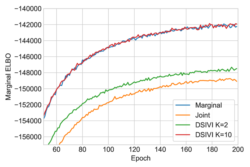
It means that if the likelihood function does not depend on the hyperparameters α𝛼\alpha, it is beneficial to consider the semi-implicit formulation instead of the joint formulation of variational inference even if the approximation family stays exactly the same. In the experiments, we show that the proposed DSIVI procedure matches the performance of direct optimization of marginalsuperscript𝑚𝑎𝑟𝑔𝑖𝑛𝑎𝑙\mathcal{L}^{marginal}, whereas joint VI performs much worse.

6 EXPERIMENTS

6.1 Variational Inference with Hierarchical Priors

We consider a Bayesian neural network with a fully-factorized hierarchical prior distribution with a Gaussian conditional p(wij|αij)=𝒩(wij| 0,αij1)𝑝conditionalsubscript𝑤𝑖𝑗subscript𝛼𝑖𝑗𝒩conditionalsubscript𝑤𝑖𝑗 0superscriptsubscript𝛼𝑖𝑗1p(w_{ij}\,|\,\alpha_{ij})=\mathcal{N}(w_{ij}\,|\,0,\alpha_{ij}^{-1}) and a Gamma hyperprior over the inverse variances p(αij)=Gamma(αij| 0.5,2)𝑝subscript𝛼𝑖𝑗Gammaconditionalsubscript𝛼𝑖𝑗0.52p(\alpha_{ij})=\mathrm{Gamma}(\alpha_{ij}\,|\,0.5,2). Such hierarchical prior induces a fully-factorized Student’s t-distribution with one degree of freedom as the marginal prior p(wij)=t(wij|ν=1)𝑝subscript𝑤𝑖𝑗𝑡conditionalsubscript𝑤𝑖𝑗𝜈1p(w_{ij})=t(w_{ij}\,|\,\nu=1). Note that in this case, we can estimate the marginal evidence lower bound directly. We consider a fully-connected neural network with two hidden layers of 300 and 100 neurons on the MNIST dataset [16]. We train all methods with the same hyperparameters: we use batch size 200, use Adam optimizer [13] with default parameters, starting with learning rate 103superscript10310^{-3}, and train for 200 epochs, using linear learning rate decay.

We consider three different ways to perform inference in this model, the marginal inference, the joint inference, and DSIVI, as described in Section 5.2. For joint inference, we consider a fully-factorized joint approximate posterior qϕ(w,α)=qϕ(w)qϕ(α)subscript𝑞italic-ϕ𝑤𝛼subscript𝑞italic-ϕ𝑤subscript𝑞italic-ϕ𝛼q_{\phi}(w,\alpha)=q_{\phi}(w)q_{\phi}(\alpha), with qϕ(w)subscript𝑞italic-ϕ𝑤q_{\phi}(w) being a fully-factorized Gaussian, and qϕ(α)subscript𝑞italic-ϕ𝛼q_{\phi}(\alpha) being a fully-factorized Log-Normal distribution. Such joint approximate posterior induces a fully-factorized Gaussian marginal posterior qϕ(w)subscript𝑞italic-ϕ𝑤q_{\phi}(w). Therefore, we use a fully-factorized Gaussian posterior for the marginal inference and DSIVI. Note that in this case, only the prior distribution is semi-implicit. All models have been trained with the local reparameterization trick [14].

We perform inference using these three different variational objectives, and then compare the true evidence lower bound marginalsuperscript𝑚𝑎𝑟𝑔𝑖𝑛𝑎𝑙\mathcal{L}^{marginal} on the training set. As the marginal variational approximation is the same in all four cases, the training ELBO can act as a proxy metric for the KL-divergence between the marginal approximate posterior and the true marginal posterior. The results are presented in Figure 1. DSIVI with as low as K=10𝐾10K=10 samples during training exactly matches the performance of the true marginal variational inference, whereas other approximations fall far behind. All three methods achieve 97.798.0%97.7percent98.097.7-98.0\% test set accuracy, and the test log-likelihood is approximately the same for all methods, ranging from 830830-830 to 855855-855. However, the difference in the marginal ELBO is high. The final values of the ELBO, its decomposition into train log-likelihood and the KL term, and the test log-likelihood are presented in Table 2 in Appendix C.
Refer to caption
Figure 1: Variational inference with a hierarchical prior. Models are trained using different variational objectives. The estimates of the marginal evidence lower bound are presented in this plot.

6.2 Comparison to Alternatives

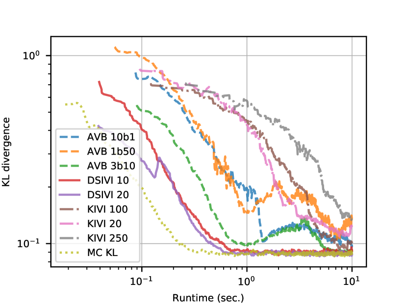
We compare DSIVI to other methods for implicit VI on a toy problem of approximating a centered standard Student’s t-distribution p(z)𝑝𝑧p(z) with 1 degrees of freedom with a Laplace distribution qϕ(z)subscript𝑞italic-ϕ𝑧q_{\phi}(z) by representing them as scale mixtures of Gaussians. Namely, we represent p(z)=𝒩(z| 0,α1)Gamma(α| 0.5,2)𝑑α𝑝𝑧𝒩conditional𝑧 0superscript𝛼1Gammaconditional𝛼0.52differential-d𝛼p(z)=\int\mathcal{N}(z\,|\,0,\alpha^{-1})\mathrm{Gamma}(\alpha\,|\,0.5,2)\,d\alpha, and qϕ(z)=𝒩(z|μ,τ)Exp(τ|λ)𝑑τsubscript𝑞italic-ϕ𝑧𝒩conditional𝑧𝜇𝜏Expconditional𝜏𝜆differential-d𝜏q_{\phi}(z)=\int\mathcal{N}(z\,|\,\mu,\tau)\mathrm{Exp}(\tau\,|\,\lambda)\,d\tau. We train all methods by minimizing the corresponding approximations to the KL-divergence KL(qϕ(z)p(z))KLconditionalsubscript𝑞italic-ϕ𝑧𝑝𝑧{\mathrm{KL}}(q_{\phi}(z)\,\|\,p(z)) w.r.t. the parameters μ𝜇\mu and λ𝜆\lambda of the approximation qϕ(z)subscript𝑞italic-ϕ𝑧q_{\phi}(z).

As baselines, we use prior methods for implicit VI: Adversarial Variational Bayes (AVB) [21], which is a discriminator-based method, and Kernel Implicit Variational Inference (KIVI) [31]. For AVB we fix architecture of the “discriminator” neural network to have 2 hidden layers with 3 and 4 hidden units with LeakyReLU (α=0.2𝛼0.2\alpha=0.2) activation, and for KIVI we use fixed λ=0.001𝜆0.001\lambda=0.001 with varying number of samples. For AVB we tried different numbers of training samples and optimization steps to optimize the discriminator at each step of optimizing over ϕitalic-ϕ\phi. We used Adam optimizer with learning rate 102superscript10210^{-2} and one MC sample to estimate gradients w.r.t. ϕitalic-ϕ\phi.

We report the KL-divergence KL(qϕ(z)p(z))𝐾𝐿conditionalsubscript𝑞italic-ϕ𝑧𝑝𝑧KL(q_{\phi}(z)\,\|\,p(z)), estimated using 10000 MC samples averaged over 10 runs. The results are presented in Figure 2. DSIVI converges faster, is more stable, and only has one hyperparameter, the number of samples K𝐾K in the DSIVI objective.

Refer to caption
Figure 2: Comparison of different techniques for (semi-)implicit VI. “KIVI K” corresponds to KIVI, K being the number of MC samples, used to approximate KL divergence; “DSIVI K” corresponds to DSIVI with K=K; “AVB MbK” corresponds to AVB with M updates of discriminator per one update of ϕitalic-ϕ\phi and K MC samples to estimate the discriminator’s gradients. “MC KL” corresponds to direct stochastic minimization of the KL divergence.

6.3 Sequential Approximation

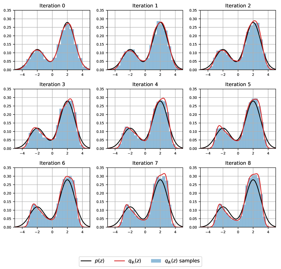
We illustrate the expressiveness of DSIVI with implicit prior and posterior distributions on the following toy problem. Consider an explicit distribution p(z)𝑝𝑧p(z). We would like to learn a semi-implicit distribution qϕ1(z)=𝔼qϕ1(ψ)[qϕ1(z|ψ)]subscript𝑞subscriptitalic-ϕ1𝑧subscript𝔼subscript𝑞subscriptitalic-ϕ1𝜓delimited-[]subscript𝑞subscriptitalic-ϕ1conditional𝑧𝜓q_{\phi_{1}}(z)=\mathbb{E}_{q_{\phi_{1}}(\psi)}[q_{\phi_{1}}(z\,|\,\psi)] to match p(z)𝑝𝑧p(z). During the first step, we apply DSIVI to tune the parameters ϕ1subscriptitalic-ϕ1\phi_{1} so as to minimize KL(qϕ1(z)p(z))KLconditionalsubscript𝑞subscriptitalic-ϕ1𝑧𝑝𝑧{\mathrm{KL}}(q_{\phi_{1}}(z)\,\|\,p(z)). Then, we take the trained semi-implicit qϕ1(z)subscript𝑞subscriptitalic-ϕ1𝑧q_{\phi_{1}}(z) as a new target for z𝑧z and tune ϕ2subscriptitalic-ϕ2\phi_{2} minimizing KL(qϕ2(z)qϕ1(z))KLconditionalsubscript𝑞subscriptitalic-ϕ2𝑧subscript𝑞subscriptitalic-ϕ1𝑧{\mathrm{KL}}(q_{\phi_{2}}(z)\,\|\,q_{\phi_{1}}(z)). After we repeat the iterative process k𝑘k times, qϕk(z)subscript𝑞subscriptitalic-ϕ𝑘𝑧q_{\phi_{k}}(z) obtained through minimization of KL(qϕk(z)qϕk1(z))KLconditionalsubscript𝑞subscriptitalic-ϕ𝑘𝑧subscript𝑞subscriptitalic-ϕ𝑘1𝑧{\mathrm{KL}}(q_{\phi_{k}}(z)\,\|\,q_{\phi_{k-1}}(z)) should still match p(z)𝑝𝑧p(z).

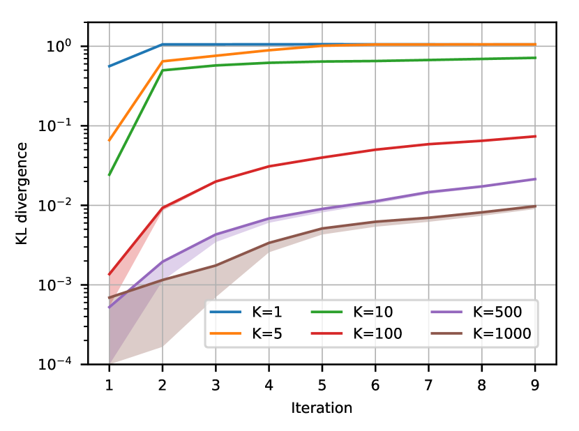
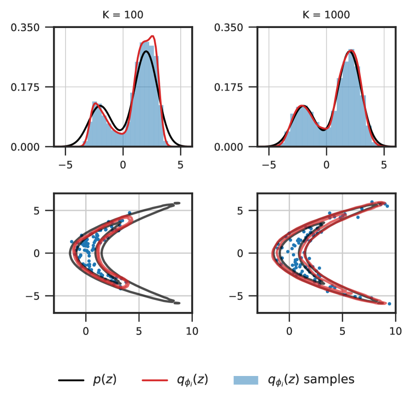
In our experiments, we follow [40] and model qϕi(ψ)subscript𝑞subscriptitalic-ϕ𝑖𝜓q_{\phi_{i}}(\psi) by a multi-layer perceptron (MLP) with layer widths [30,60,30] with ReLU activations and a ten-dimensional standard normal noise as its input. We also fix all conditionals qϕi(z|ψ)=𝒩(z|ψ,σ2I)subscript𝑞subscriptitalic-ϕ𝑖conditional𝑧𝜓𝒩conditional𝑧𝜓superscript𝜎2𝐼q_{\phi_{i}}(z\,|\,\psi)=\mathcal{N}(z\,|\,\psi,\sigma^{2}I), σ2=0.1superscript𝜎20.1\sigma^{2}=0.1. We choose p(z)𝑝𝑧p(z) to be either a one-dimensional mixture of Gaussians or a two-dimensional “banana” distribution. In Figure 3 we plot values of KL(qϕi(z)p(z))KLconditionalsubscript𝑞subscriptitalic-ϕ𝑖𝑧𝑝𝑧{\mathrm{KL}}(q_{\phi_{i}}(z)\,\|\,p(z)), i=1,,9𝑖19i=1,\dotsc,9 for different values of K1=K2=Ksubscript𝐾1subscript𝐾2𝐾K_{1}=K_{2}=K (see Algorithm 1) when p(z)𝑝𝑧p(z) is a one-dimensional mixture of Gaussians (see Appendix D for a detailed description and additional plots). In Figure 4 we plot the approximate PDF of qϕk(z)subscript𝑞subscriptitalic-ϕ𝑘𝑧q_{\phi_{k}}(z) after 9 steps for different values of K𝐾K. As we can see, even though both “prior” and “posterior” distributions are semi-implicit, the algorithm can still accurately learn the original target distribution after several iterations.
Refer to caption
Figure 3: Sequential approximation. Area is shaded between lower and upper bounds of KL(qϕi(z)p(z))KLconditionalsubscript𝑞subscriptitalic-ϕ𝑖𝑧𝑝𝑧{\mathrm{KL}}(q_{\phi_{i}}(z)\,\|\,p(z)) for different training values of K1=K2=Ksubscript𝐾1subscript𝐾2𝐾K_{1}=K_{2}=K, and the solid lines represent the corresponding upper bounds. During evaluation, K=104𝐾superscript104K=10^{4} is used. Here p(z)𝑝𝑧p(z) is a one dimensional Gaussian mixture (see Appendix D for details.) Lower is better.
Refer to caption
Figure 4: Learned probability distributions qϕk(z)subscript𝑞subscriptitalic-ϕ𝑘𝑧q_{\phi_{k}}(z) after 9 iterations of sequential approximation for K1=K2=100subscript𝐾1subscript𝐾2100K_{1}=K_{2}=100 and 100010001000 (red), and the two original priors p(z)𝑝𝑧p(z) (black). During evaluation, K=104𝐾superscript104K=10^{4}.

6.4 VAE with Semi-Implicit Optimal Prior

We follow the same experimental setup and use the same hyperparameters, as suggested for VampPrior [35]. We consider two architectures, the VAE and the HVAE (hierarchical VAE, [35]), applied to the MNIST dataset with dynamic binarization [28]. In both cases, all distributions (except the prior) have been modeled by fully-factorized neural networks with two hidden layers of 300 hidden units each. We used 40-dimensional latent vectors z𝑧z (40-dimensional z1subscript𝑧1z_{1} and z2subscript𝑧2z_{2} for HVAE) and Bernoulli likelihood with dynamic binarization for the MNIST dataset. As suggested in the VampPrior paper, we used 500 pseudo-inputs for VampPrior-based models in all cases (higher number of pseudo-inputs led to overfitting). To measure the performance of all models, we bound the test log-likelihood with the IWAE objective [4] with 5000 samples for the VampPrior-based methods, and estimate the corresponding IW-DSIVAE lower bound with K=20000𝐾20000K=20000 for the DSIVI-based methods (see Appendix B for more details).

Table 1: We compare VampPrior with its semi-implicit modifications, DSIVI-agg and DSIVI-prior. We report the the IWAE objective Ssuperscript𝑆\mathcal{L}^{S} for VampPrior-data, and the corresponding lower bound ¯Kp,Ssuperscriptsubscript¯𝐾𝑝𝑆\underline{\mathcal{L}}_{K}^{p,S} for DSIVI-based methods (see Appendix B). Only the prior distribution is semi-implicit.
Method LL
VAE+VampPrior-data 85.0585.05-85.05
VAE+VampPrior 82.3882.38-82.38
VAE+DSIVI-prior (K=2000) 82.27absent82.27\geq-82.27
VAE+DSIVI-agg (K=500) 83.02absent83.02\geq-83.02
VAE+DSIVI-agg (K=5000) 82.16absent82.16\geq\mathbf{-82.16}
HVAE+VampPrior-data 81.7181.71-81.71
HVAE+VampPrior 81.2481.24-81.24
HVAE+DSIVI-agg (K=5000) 81.09absent81.09\geq\mathbf{-81.09}

We consider two formulations, described in Section 5.1: DSIVI-agg stands for the semi-implicit formulation of the aggregated posterior (28), and DSIVI-prior stands for a general semi-implicit prior (30). For the DSIVI-prior we have used a fully-factorized Gaussian conditional p(z|ζ)=𝒩(z|ζ,diag(σ2))𝑝conditional𝑧𝜁𝒩conditional𝑧𝜁diagsuperscript𝜎2p(z\,|\,\zeta)=\mathcal{N}(z\,|\,\zeta,\mathrm{diag}(\sigma^{2})), where the mixing parameters ζ𝜁\zeta are the output of a fully-connected neural network with two hidden layers with 300 and 600 hidden units respectively, applied to a 300-dimensional standard Gaussian noise ϵitalic-ϵ\epsilon. The first and second hidden layers were followed by ReLU non-linearities, and no non-linearities were applied to obtain ζ𝜁\zeta. We did not use warm-up [35] with DSIVI-prior.

The results are presented in Table 1. DSIVI-agg is a simple modification of VampPrior-data that significantly improves the test log-likelihood, and even outperforms the VampPrior with trained inducing inputs. DSIVI-prior outperforms VampPrior even without warm-up and without coupling the parameters of the prior and the variational posteriors.

7 CONCLUSION

We have presented DSIVI, a general-purpose framework that allows to perform variational inference and variational learning when both the approximate posterior distribution and the prior distribution are semi-implicit. DSIVI provides an asymptotically exact lower bound on the ELBO, and also an upper bound that can be made arbitrarily tight. It allows us to estimate the ELBO in any model with semi-implicit distributions, which was not the case for other methods. We have shown the effectiveness of DSIVI applied to a range of problems, e.g. models with hierarchical priors and variational autoencoders with semi-implicit empirical priors. In particular, we show how DSIVI-based treatment improves the performance of VampPrior, the current state-of-the-art prior distribution for VAE.

ACKNOWLEDGMENTS

We would like to thank Arsenii Ashukha and Kirill Neklyudov for valuable discussions. Dmitry Molchanov and Valery Kharitonov were supported by Samsung Research, Samsung Electronics.

References

  • [1] A. Alemi, B. Poole, I. Fischer, J. Dillon, R. A. Saurous, and K. Murphy. Fixing a broken elbo. In International Conference on Machine Learning, pages 159–168, 2018.
  • [2] A. Atanov, A. Ashukha, K. Struminsky, D. Vetrov, and M. Welling. The deep weight prior. In International Conference on Learning Representations, 2019.
  • [3] D. M. Blei, A. Kucukelbir, and J. D. McAuliffe. Variational inference: A review for statisticians. Journal of the American Statistical Association, 112(518):859–877, 2017.
  • [4] Y. Burda, R. Grosse, and R. Salakhutdinov. Importance weighted autoencoders. arXiv preprint arXiv:1509.00519, 2015.
  • [5] R. J. Giordano, T. Broderick, and M. I. Jordan. Linear response methods for accurate covariance estimates from mean field variational bayes. In Advances in Neural Information Processing Systems, pages 1441–1449, 2015.
  • [6] S. Han, X. Liao, D. Dunson, and L. Carin. Variational gaussian copula inference. In Artificial Intelligence and Statistics, pages 829–838, 2016.
  • [7] J. M. Hernández-Lobato and R. Adams. Probabilistic backpropagation for scalable learning of bayesian neural networks. In International Conference on Machine Learning, pages 1861–1869, 2015.
  • [8] I. Higgins, L. Matthey, A. Pal, C. Burgess, X. Glorot, M. Botvinick, S. Mohamed, and A. Lerchner. β𝛽\beta-vae: Learning basic visual concepts with a constrained variational framework. 2016.
  • [9] M. D. Hoffman and D. M. Blei. Structured stochastic variational inference. In Artificial Intelligence and Statistics, 2015.
  • [10] M. D. Hoffman and M. J. Johnson. Elbo surgery: yet another way to carve up the variational evidence lower bound. In Workshop in Advances in Approximate Bayesian Inference, NIPS, 2016.
  • [11] F. Huszár. Variational inference using implicit distributions. arXiv preprint arXiv:1702.08235, 2017.
  • [12] T. S. Jaakkola and M. I. Jordan. Improving the mean field approximation via the use of mixture distributions. In Learning in graphical models, pages 163–173. Springer, 1998.
  • [13] D. P. Kingma and J. Ba. Adam: A method for stochastic optimization. arXiv preprint arXiv:1412.6980, 2014.
  • [14] D. P. Kingma, T. Salimans, and M. Welling. Variational dropout and the local reparameterization trick. In Advances in Neural Information Processing Systems, pages 2575–2583, 2015.
  • [15] D. P. Kingma and M. Welling. Auto-encoding variational bayes. arXiv preprint arXiv:1312.6114, 2013.
  • [16] Y. LeCun, L. Bottou, Y. Bengio, and P. Haffner. Gradient-based learning applied to document recognition. Proceedings of the IEEE, 86(11):2278–2324, 1998.
  • [17] Y. Li and R. E. Turner. Gradient estimators for implicit models. arXiv preprint arXiv:1705.07107, 2017.
  • [18] C. Louizos, K. Ullrich, and M. Welling. Bayesian compression for deep learning. In Advances in Neural Information Processing Systems, pages 3288–3298, 2017.
  • [19] C. Louizos and M. Welling. Multiplicative normalizing flows for variational bayesian neural networks. arXiv preprint arXiv:1703.01961, 2017.
  • [20] L. Maaløe, C. K. Sønderby, S. K. Sønderby, and O. Winther. Auxiliary deep generative models. In M. F. Balcan and K. Q. Weinberger, editors, Proceedings of The 33rd International Conference on Machine Learning, volume 48 of Proceedings of Machine Learning Research, pages 1445–1453, New York, New York, USA, 20–22 Jun 2016. PMLR.
  • [21] L. Mescheder, S. Nowozin, and A. Geiger. Adversarial variational bayes: Unifying variational autoencoders and generative adversarial networks. ICML, 2017.
  • [22] S. Mohamed and B. Lakshminarayanan. Learning in implicit generative models. arXiv preprint arXiv:1610.03483, 2016.
  • [23] R. M. Neal. Bayesian learning for neural networks, volume 118. 1995.
  • [24] K. Neklyudov, D. Molchanov, A. Ashukha, and D. P. Vetrov. Structured bayesian pruning via log-normal multiplicative noise. In Advances in Neural Information Processing Systems, pages 6775–6784, 2017.
  • [25] X. Nguyen, M. J. Wainwright, and M. I. Jordan. Estimating divergence functionals and the likelihood ratio by convex risk minimization. IEEE Transactions on Information Theory, 56(11):5847–5861, 2010.
  • [26] R. Ranganath, D. Tran, J. Altosaar, and D. Blei. Operator variational inference. In Advances in Neural Information Processing Systems, pages 496–504, 2016.
  • [27] R. Ranganath, D. Tran, and D. Blei. Hierarchical variational models. In International Conference on Machine Learning, pages 324–333, 2016.
  • [28] R. Salakhutdinov and I. Murray. On the quantitative analysis of deep belief networks. In Proceedings of the 25th international conference on Machine learning, pages 872–879. ACM, 2008.
  • [29] T. Salimans, D. Kingma, and M. Welling. Markov chain monte carlo and variational inference: Bridging the gap. In International Conference on Machine Learning, pages 1218–1226, 2015.
  • [30] L. K. Saul and M. I. Jordan. Exploiting tractable substructures in intractable networks. In Advances in neural information processing systems, pages 486–492, 1996.
  • [31] J. Shi, S. Sun, and J. Zhu. Kernel implicit variational inference. arXiv preprint arXiv:1705.10119, 2017.
  • [32] M. Sugiyama, T. Suzuki, and T. Kanamori. Density ratio estimation in machine learning. Cambridge University Press, 2012.
  • [33] M. Tipping. Sparse Bayesian Learning and the Relevance Vector Machine. 1:211–244, 2000.
  • [34] M. Titsias and M. Lázaro-Gredilla. Doubly stochastic variational bayes for non-conjugate inference. In International Conference on Machine Learning, pages 1971–1979, 2014.
  • [35] J. M. Tomczak and M. Welling. Vae with a vampprior. arXiv preprint arXiv:1705.07120, 2017.
  • [36] D. Tran, D. Blei, and E. M. Airoldi. Copula variational inference. In Advances in Neural Information Processing Systems, pages 3564–3572, 2015.
  • [37] D. Tran, R. Ranganath, and D. Blei. Hierarchical implicit models and likelihood-free variational inference. In Advances in Neural Information Processing Systems, pages 5523–5533, 2017.
  • [38] D. Tran, R. Ranganath, and D. M. Blei. The variational gaussian process. ICLR, 2016.
  • [39] B. Trippe and R. Turner. Overpruning in variational bayesian neural networks. arXiv preprint arXiv:1801.06230, 2018.
  • [40] M. Yin and M. Zhou. Semi-implicit variational inference. In Proceedings of the 35th International Conference on Machine Learning, volume 80, pages 5660–5669. PMLR, 2018.

Appendix A Proof of the SIVI Lower Bound for Semi-Implicit Posteriors

Theorem 1.

Consider \mathcal{L} and ¯Kqsuperscriptsubscript¯𝐾𝑞\underline{\mathcal{L}}_{K}^{q} defined as in Eq. (2) and (6). Then ¯Kqsuperscriptsubscript¯𝐾𝑞\underline{\mathcal{L}}_{K}^{q} converges to \mathcal{L} from below as K𝐾K\to~{}\infty, satisfying ¯Kq¯K+1qsuperscriptsubscript¯𝐾𝑞superscriptsubscript¯𝐾1𝑞\underline{\mathcal{L}}_{K}^{q}\leq\underline{\mathcal{L}}_{K+1}^{q}\leq\mathcal{L}, and

¯Kq=𝔼ψ0..Kqϕ(ψ)𝔼qϕK(z|ψ0..K)logp(x|z)p(z)qϕK(z|ψ0..K),\displaystyle\underline{\mathcal{L}}_{K}^{q}=\mathbb{E}_{\psi^{0..K}\sim q_{\phi}(\psi)}\mathbb{E}_{q_{\phi}^{K}(z\,|\,\psi^{0..K})}\log{\frac{p(x\,|\,z)p(z)}{q_{\phi}^{K}(z\,|\,\psi^{0..K})}}, (36)
where qϕK(z|ψ0..K)=1K+1k=0Kqϕ(z|ψk).\displaystyle\text{where }q_{\phi}^{K}(z\,|\,\psi^{0..K})=\frac{1}{K+1}\sum_{k=0}^{K}q_{\phi}(z\,|\,\psi^{k}). (37)
Proof.

For brevity, we denote 𝔼ψ0..Kqϕ(ψ)\mathbb{E}_{\psi^{0..K}\sim q_{\phi}(\psi)} as 𝔼ψ0..K\mathbb{E}_{\psi^{0..K}} and 𝔼zqϕK(z|ψ0..K)\mathbb{E}_{z\sim q_{\phi}^{K}(z\,|\,\psi^{0..K})} as 𝔼z|ψ0..K\mathbb{E}_{z\,|\,\psi^{0..K}}. First, notice that due to the symmetry in the indices, the regularized lower bound ¯Kqsuperscriptsubscript¯𝐾𝑞\underline{\mathcal{L}}_{K}^{q} does not depend on the index in the conditional qϕ(z|ψi)subscript𝑞italic-ϕconditional𝑧superscript𝜓𝑖q_{\phi}(z\,|\,\psi^{i}):

¯Kqsuperscriptsubscript¯𝐾𝑞\displaystyle\underline{\mathcal{L}}_{K}^{q} =𝔼ψ0..K𝔼z|ψ0logp(x,z)qϕK(z|ψ0..K)=\displaystyle=\mathbb{E}_{\psi^{0..K}}\mathbb{E}_{z\,|\,\psi^{0}}\log\frac{p(x,z)}{q_{\phi}^{K}(z\,|\,\psi^{0..K})}= (38)
=𝔼ψ0..K𝔼z|ψilogp(x,z)qϕK(z|ψ0..K).\displaystyle=\mathbb{E}_{\psi^{0..K}}\mathbb{E}_{z\,|\,\psi^{i}}\log\frac{p(x,z)}{q_{\phi}^{K}(z\,|\,\psi^{0..K})}. (39)

Therefore, we can rewrite ¯Kqsuperscriptsubscript¯𝐾𝑞\underline{\mathcal{L}}_{K}^{q} as follows:

¯Kq=1K+1i=0K¯Kq=superscriptsubscript¯𝐾𝑞1𝐾1superscriptsubscript𝑖0𝐾superscriptsubscript¯𝐾𝑞absent\displaystyle\underline{\mathcal{L}}_{K}^{q}=\frac{1}{K+1}\sum_{i=0}^{K}\underline{\mathcal{L}}_{K}^{q}= (40)
=1K+1i=0K𝔼ψ0..K𝔼z|ψilogp(x,z)qϕK(z|ψ0..K)=\displaystyle=\frac{1}{K+1}\sum_{i=0}^{K}\mathbb{E}_{\psi^{0..K}}\mathbb{E}_{z\,|\,\psi^{i}}\log\frac{p(x,z)}{q_{\phi}^{K}(z\,|\,\psi^{0..K})}= (41)
=𝔼ψ0..K𝔼z|ψ0..Klogp(x,z)qϕK(z|ψ0..K).\displaystyle=\mathbb{E}_{\psi^{0..K}}\mathbb{E}_{z\,|\,\psi^{0..K}}\log\frac{p(x,z)}{q_{\phi}^{K}(z\,|\,\psi^{0..K})}. (42)

Note that it is just the value of the evidence lower bound with the approximate posterior qϕK(z|ψ0..K)q_{\phi}^{K}(z\,|\,\psi^{0..K}), averaged over all values of ψ0..K\psi^{0..K}. We can also use that 𝔼ψ0..KqϕK(z|ψ0..K)=qϕ(z)\mathbb{E}_{\psi^{0..K}}q_{\phi}^{K}(z\,|\,\psi^{0..K})=q_{\phi}(z) to rewrite the true ELBO in the same expectations:

=𝔼qϕ(z)logp(x,z)qϕ(z)=subscript𝔼subscript𝑞italic-ϕ𝑧𝑝𝑥𝑧subscript𝑞italic-ϕ𝑧absent\displaystyle\mathcal{L}=\mathbb{E}_{q_{\phi}(z)}\log\frac{p(x,z)}{q_{\phi}(z)}= (43)
=𝔼ψ0..K𝔼z|ψ0..Klogp(x,z)qϕ(z).\displaystyle=\mathbb{E}_{\psi^{0..K}}\mathbb{E}_{z\,|\,\psi^{0..K}}\log\frac{p(x,z)}{q_{\phi}(z)}. (44)

We want to prove that ¯Kqsuperscriptsubscript¯𝐾𝑞\mathcal{L}\geq\underline{\mathcal{L}}_{K}^{q}. Consider their difference ¯Kqsuperscriptsubscript¯𝐾𝑞\mathcal{L}-\underline{\mathcal{L}}_{K}^{q}:

¯Kq=superscriptsubscript¯𝐾𝑞absent\displaystyle\mathcal{L}-\underline{\mathcal{L}}_{K}^{q}= (45)
=𝔼ψ0..K𝔼z|ψ0..KlogqϕK(z|ψ0..K)qϕ(z)=\displaystyle=\mathbb{E}_{\psi^{0..K}}\mathbb{E}_{z\,|\,\psi^{0..K}}\log\frac{q_{\phi}^{K}(z\,|\,\psi^{0..K})}{q_{\phi}(z)}= (46)
=𝔼ψ0..KKL(qϕK(z|ψ0..K)qϕ(z))0.\displaystyle=\mathbb{E}_{\psi^{0..K}}{\mathrm{KL}}\left(q_{\phi}^{K}(z\,|\,\psi^{0..K})\,\|\,q_{\phi}(z)\right)\geq 0. (47)

We can use the same trick to prove that this bound is non-decreasing in K𝐾K. First, let’s use the symmetry in the indices once again, and rewrite ¯Kqsuperscriptsubscript¯𝐾𝑞\underline{\mathcal{L}}_{K}^{q} and ¯K+1qsuperscriptsubscript¯𝐾1𝑞\underline{\mathcal{L}}_{K+1}^{q} in the same expectations:

¯Kq=𝔼ψ0..K𝔼z|ψ0..Klogp(x,z)qϕK(z|ψ0..K)=\displaystyle\underline{\mathcal{L}}_{K}^{q}=\mathbb{E}_{\psi^{0..K}}\mathbb{E}_{z\,|\,\psi^{0..K}}\log\frac{p(x,z)}{q_{\phi}^{K}(z\,|\,\psi^{0..K})}= (48)
=𝔼ψ0..K+1𝔼z|ψ0..Klogp(x,z)qϕK(z|ψ0..K),\displaystyle=\mathbb{E}_{\psi^{0..K+1}}\mathbb{E}_{z\,|\,\psi^{0..K}}\log\frac{p(x,z)}{q_{\phi}^{K}(z\,|\,\psi^{0..K})}, (49)
¯K+1q=𝔼ψ0..K+1𝔼z|ψ0logp(x,z)qϕK+1(z|ψ0..K+1)=\displaystyle\underline{\mathcal{L}}_{K+1}^{q}=\mathbb{E}_{\psi^{0..K+1}}\mathbb{E}_{z\,|\,\psi^{0}}\log\frac{p(x,z)}{q_{\phi}^{K+1}(z\,|\,\psi^{0..K+1})}= (50)
=𝔼ψ0..K+1𝔼z|ψ0..Klogp(x,z)qϕK+1(z|ψ0..K+1).\displaystyle=\mathbb{E}_{\psi^{0..K+1}}\mathbb{E}_{z\,|\,\psi^{0..K}}\log\frac{p(x,z)}{q_{\phi}^{K+1}(z\,|\,\psi^{0..K+1})}. (51)

Then their difference would be equal to the expected KL-divergence, hence being non-negative:

¯K+1q¯Kq=superscriptsubscript¯𝐾1𝑞superscriptsubscript¯𝐾𝑞absent\displaystyle\underline{\mathcal{L}}_{K+1}^{q}-\underline{\mathcal{L}}_{K}^{q}= (52)
=𝔼ψ0..K+1𝔼z|ψ0..KlogqϕK(z|ψ0..K)qϕK+1(z|ψ0..K+1)=\displaystyle=\mathbb{E}_{\psi^{0..K+1}}\mathbb{E}_{z\,|\,\psi^{0..K}}\log\frac{q_{\phi}^{K}(z\,|\,\psi^{0..K})}{q_{\phi}^{K+1}(z\,|\,\psi^{0..K+1})}= (53)
=𝔼ψ0..K+1KL(qϕK(z|ψ0..K)qϕK+1(z|ψ0..K+1)))\displaystyle=\mathbb{E}_{\psi^{0..K+1}}{\mathrm{KL}}\left(q_{\phi}^{K}(z\,|\,\psi^{0..K})\,\|\,q_{\phi}^{K+1}(z\,|\,\psi^{0..K+1}))\right)
0.absent0\displaystyle\geq 0.

Appendix B Importance Weighted Doubly Semi-Implicit VAE

The standard importance-weighted lower bound for VAE is defined as follows:

logp(x)S=𝔼z1..Sqϕ(z)log1Si=1Sp(x|zi)p(zi)qϕ(zi|x)\log p(x)\geq\mathcal{L}^{S}=\mathbb{E}_{z^{1..S}\sim q_{\phi}(z)}\log\frac{1}{S}\sum_{i=1}^{S}\frac{p(x\,|\,z^{i})p(z^{i})}{q_{\phi}(z_{i}\,|\,x)} (54)

We propose IW-DSIVAE, a new lower bound on the IWAE objective, that is suitable for VAEs with semi-implicit priors and posteriors:

¯¯K1,K2q,p,S=𝔼ψ1..K1qϕ(ψ)𝔼ζ1..K2pθ(ζ)[𝔼(z1,ψ^1),,(zS,ψ^S)qϕ(z,ψ)[log1Si=1Sp(x|zi)1K2k=1K2pθ(zi|ζk)1K1+1(qϕ(zi|ψ^i)+k=1K1qϕ(zi|ψk))]].\displaystyle\begin{multlined}\underline{\underline{\mathcal{L}}}_{K_{1},K_{2}}^{q,p,S}=\mathbb{E}_{\psi^{1..K_{1}}\sim q_{\phi}(\psi)}\mathbb{E}_{\zeta^{1..K_{2}}\sim p_{\theta}(\zeta)}\left[\phantom{\frac{1}{S}}\right.\\ \mathbb{E}_{(z^{1},\hat{\psi}^{1}),\dots,(z^{S},\hat{\psi}^{S})\sim q_{\phi}(z,\psi)}\left[\phantom{\frac{1}{S}}\right.\\ \left.\left.\log\frac{1}{S}\sum_{i=1}^{S}\frac{p(x\,|\,z^{i})\frac{1}{K_{2}}\sum_{k=1}^{K_{2}}p_{\theta}(z^{i}\,|\,\zeta^{k})}{\frac{1}{K_{1}+1}(q_{\phi}(z^{i}\,|\,\hat{\psi}^{i})+\sum_{k=1}^{K_{1}}q_{\phi}(z^{i}\,|\,\psi^{k}))}\right]\right].\end{multlined}\underline{\underline{\mathcal{L}}}_{K_{1},K_{2}}^{q,p,S}=\mathbb{E}_{\psi^{1..K_{1}}\sim q_{\phi}(\psi)}\mathbb{E}_{\zeta^{1..K_{2}}\sim p_{\theta}(\zeta)}\left[\phantom{\frac{1}{S}}\right.\\ \mathbb{E}_{(z^{1},\hat{\psi}^{1}),\dots,(z^{S},\hat{\psi}^{S})\sim q_{\phi}(z,\psi)}\left[\phantom{\frac{1}{S}}\right.\\ \left.\left.\log\frac{1}{S}\sum_{i=1}^{S}\frac{p(x\,|\,z^{i})\frac{1}{K_{2}}\sum_{k=1}^{K_{2}}p_{\theta}(z^{i}\,|\,\zeta^{k})}{\frac{1}{K_{1}+1}(q_{\phi}(z^{i}\,|\,\hat{\psi}^{i})+\sum_{k=1}^{K_{1}}q_{\phi}(z^{i}\,|\,\psi^{k}))}\right]\right]. (58)

This objective is a lower bound on the IWAE objective (¯¯K1,K2q,p,SSsuperscriptsubscript¯¯subscript𝐾1subscript𝐾2𝑞𝑝𝑆superscript𝑆\underline{\underline{\mathcal{L}}}_{K_{1},K_{2}}^{q,p,S}\leq\mathcal{L}^{S}), is non-decreasing in both K1subscript𝐾1K_{1} and K2subscript𝐾2K_{2}, and is asymptotically exact (¯¯,q,p,S=Ssuperscriptsubscript¯¯𝑞𝑝𝑆superscript𝑆\underline{\underline{\mathcal{L}}}_{\infty,\infty}^{q,p,S}=\mathcal{L}^{S}).

Appendix C Variational inference with hierarchical priors

Theorem 2.

Consider two different variational objectives jointsuperscript𝑗𝑜𝑖𝑛𝑡\mathcal{L}^{joint} and marginalsuperscript𝑚𝑎𝑟𝑔𝑖𝑛𝑎𝑙\mathcal{L}^{marginal}. Then

joint(ϕ)=𝔼qϕ(w,α)logp(t|x,w)p(w|α)p(α)qϕ(w,α)superscript𝑗𝑜𝑖𝑛𝑡italic-ϕsubscript𝔼subscript𝑞italic-ϕ𝑤𝛼𝑝conditional𝑡𝑥𝑤𝑝conditional𝑤𝛼𝑝𝛼subscript𝑞italic-ϕ𝑤𝛼\displaystyle\mathcal{L}^{joint}(\phi)=\mathbb{E}_{q_{\phi}(w,\alpha)}\log\frac{p(t\,|\,x,w)p(w\,|\,\alpha)p(\alpha)}{q_{\phi}(w,\alpha)} (59)
marginal(ϕ)=𝔼qϕ(w)logp(t|x,w)p(w)qϕ(w)superscript𝑚𝑎𝑟𝑔𝑖𝑛𝑎𝑙italic-ϕsubscript𝔼subscript𝑞italic-ϕ𝑤𝑝conditional𝑡𝑥𝑤𝑝𝑤subscript𝑞italic-ϕ𝑤\displaystyle\mathcal{L}^{marginal}(\phi)=\mathbb{E}_{q_{\phi}(w)}\log\frac{p(t\,|\,x,w)p(w)}{q_{\phi}(w)} (60)

Let ϕjsubscriptitalic-ϕ𝑗\phi_{j} and ϕmsubscriptitalic-ϕ𝑚\phi_{m} maximize jointsuperscript𝑗𝑜𝑖𝑛𝑡\mathcal{L}^{joint} and marginalsuperscript𝑚𝑎𝑟𝑔𝑖𝑛𝑎𝑙\mathcal{L}^{marginal} correspondingly. Then qϕm(w)subscript𝑞subscriptitalic-ϕ𝑚𝑤q_{\phi_{m}}(w) is a better fit for the marginal posterior that qϕj(w)subscript𝑞subscriptitalic-ϕ𝑗𝑤q_{\phi_{j}}(w) in terms of the KL-divergence:

KL(qϕm(w)p(w|Xtr,Ttr))KL(qϕj(w)p(w|Xtr,Ttr)){\mathrm{KL}}(q_{\phi_{m}}(w)\,\|\,p(w\,|\,X_{tr},T_{tr}))\leq\\ {\mathrm{KL}}(\,q_{\phi_{j}}(w)\,\,\|\,p(w\,|\,X_{tr},T_{tr})) (61)
Proof.

Note that maximizing marginal(ϕ)superscript𝑚𝑎𝑟𝑔𝑖𝑛𝑎𝑙italic-ϕ\mathcal{L}^{marginal}(\phi) directly minimizes KL(qϕ(w)p(w|Xtr,Ttr)){\mathrm{KL}}(q_{\phi}(w)\,\|\,p(w\,|\,X_{tr},T_{tr})), as marginal(ϕ)+KL(qϕ(w)p(w|Xtr,Ttr))=const\mathcal{L}^{marginal}(\phi)+{\mathrm{KL}}(q_{\phi}(w)\,\|\,p(w\,|\,X_{tr},T_{tr}))=const. The sought-for inequality (61) then immediately follows from marginal(ϕm)marginal(ϕj)superscript𝑚𝑎𝑟𝑔𝑖𝑛𝑎𝑙subscriptitalic-ϕ𝑚superscript𝑚𝑎𝑟𝑔𝑖𝑛𝑎𝑙subscriptitalic-ϕ𝑗\mathcal{L}^{marginal}(\phi_{m})\geq\mathcal{L}^{marginal}(\phi_{j}). ∎

To see the cause of this inequality more clearly, consider joint(ϕ)superscript𝑗𝑜𝑖𝑛𝑡italic-ϕ\mathcal{L}^{joint}(\phi):

joint(ϕ)=𝔼qϕ(w,α)logp(t|x,w)p(w|α)p(α)qϕ(w,α)=superscript𝑗𝑜𝑖𝑛𝑡italic-ϕsubscript𝔼subscript𝑞italic-ϕ𝑤𝛼𝑝conditional𝑡𝑥𝑤𝑝conditional𝑤𝛼𝑝𝛼subscript𝑞italic-ϕ𝑤𝛼absent\displaystyle\mathcal{L}^{joint}(\phi)=\mathbb{E}_{q_{\phi}(w,\alpha)}\log\frac{p(t\,|\,x,w)p(w\,|\,\alpha)p(\alpha)}{q_{\phi}(w,\alpha)}= (62)
=𝔼qϕ(w)logp(t|x,w)KL(qϕ(w,α)p(w,α))=absentsubscript𝔼subscript𝑞italic-ϕ𝑤𝑝conditional𝑡𝑥𝑤KLconditionalsubscript𝑞italic-ϕ𝑤𝛼𝑝𝑤𝛼absent\displaystyle=\mathbb{E}_{q_{\phi}(w)}\log p(t\,|\,x,w)-{\mathrm{KL}}(q_{\phi}(w,\alpha)\,\|\,p(w,\alpha))= (63)
=𝔼qϕ(w)logp(t|x,w)KL(qϕ(w)p(w))absentsubscript𝔼subscript𝑞italic-ϕ𝑤𝑝conditional𝑡𝑥𝑤limit-fromKLconditionalsubscript𝑞italic-ϕ𝑤𝑝𝑤\displaystyle=\mathbb{E}_{q_{\phi}(w)}\log p(t\,|\,x,w)-{\mathrm{KL}}(q_{\phi}(w)\,\|\,p(w))- (64)
𝔼qϕ(w)KL(qϕ(α|w)p(α|w))=\displaystyle-\mathbb{E}_{q_{\phi}(w)}{\mathrm{KL}}(q_{\phi}(\alpha\,|\,w)\,\|\,p(\alpha\,|\,w))= (65)
=marginal(ϕ)𝔼qϕ(w)KL(qϕ(α|w)p(α|w))\displaystyle=\mathcal{L}^{marginal}(\phi)-\mathbb{E}_{q_{\phi}(w)}{\mathrm{KL}}(q_{\phi}(\alpha\,|\,w)\,\|\,p(\alpha\,|\,w)) (66)

If jointsuperscript𝑗𝑜𝑖𝑛𝑡\mathcal{L}^{joint} and marginalsuperscript𝑚𝑎𝑟𝑔𝑖𝑛𝑎𝑙\mathcal{L}^{marginal} coincide, the inequality (61) becomes an equality. However, jointsuperscript𝑗𝑜𝑖𝑛𝑡\mathcal{L}^{joint} and marginalsuperscript𝑚𝑎𝑟𝑔𝑖𝑛𝑎𝑙\mathcal{L}^{marginal} only coincide if the reverse posterior qϕ(α|w)subscript𝑞italic-ϕconditional𝛼𝑤q_{\phi}(\alpha\,|\,w) is an exact match for the reverse prior p(α|w)𝑝conditional𝛼𝑤p(\alpha\,|\,w). Due to the limitations of the approximation family of the joint posterior, this is not the case in many practical applications. In many cases [7, 18] the joint approximate posterior is modeled as a factorized distribution qϕ(w,α)=qϕ(w)qϕ(α)subscript𝑞italic-ϕ𝑤𝛼subscript𝑞italic-ϕ𝑤subscript𝑞italic-ϕ𝛼q_{\phi}(w,\alpha)=q_{\phi}(w)q_{\phi}(\alpha). Therefore in the case of the joint variational inference, we optimize a lower bound on the marginal ELBO and therefore obtain a sub-optimal approximation.

Table 2: The values of the marginal ELBO, the train negative log-likelihood, the KL-divergence between the marginal posterior qϕ(w)subscript𝑞italic-ϕ𝑤q_{\phi}(w) and the marginal prior pϕ(w)subscript𝑝italic-ϕ𝑤p_{\phi}(w), and the test-set accuracy and negative log-likelihood for different inference procedures for a model with a standard Student’s prior. The predictive distribution during test-time was estimated using 200 samples from the marginal posterior qϕ(w)subscript𝑞italic-ϕ𝑤q_{\phi}(w)
Train Test
Method ELBO NLL KL Acc. NLL
Marginal 1.42×𝟏𝟎𝟓1.42superscript105\mathbf{-1.42\times 10^{5}} 7.2×1037.2superscript1037.2\times 10^{3} 1.35×1051.35superscript1051.35\times 10^{5} 97.8097.8097.80 855855855
Joint 1.48×1051.48superscript105-1.48\times 10^{5} 6.7×1036.7superscript1036.7\times 10^{3} 1.42×1051.42superscript1051.42\times 10^{5} 97.7497.7497.74 831831831
DSIVI(K=2) 1.47×1051.47superscript105-1.47\times 10^{5} 7.0×1037.0superscript1037.0\times 10^{3} 1.41×1051.41superscript1051.41\times 10^{5} 97.7597.7597.75 846846846
DSIVI(K=10) 1.42×𝟏𝟎𝟓1.42superscript105\mathbf{-1.42\times 10^{5}} 7.2×1037.2superscript1037.2\times 10^{3} 1.35×1051.35superscript1051.35\times 10^{5} 97.7697.7697.76 843843843

Appendix D Toy data for sequential approximation

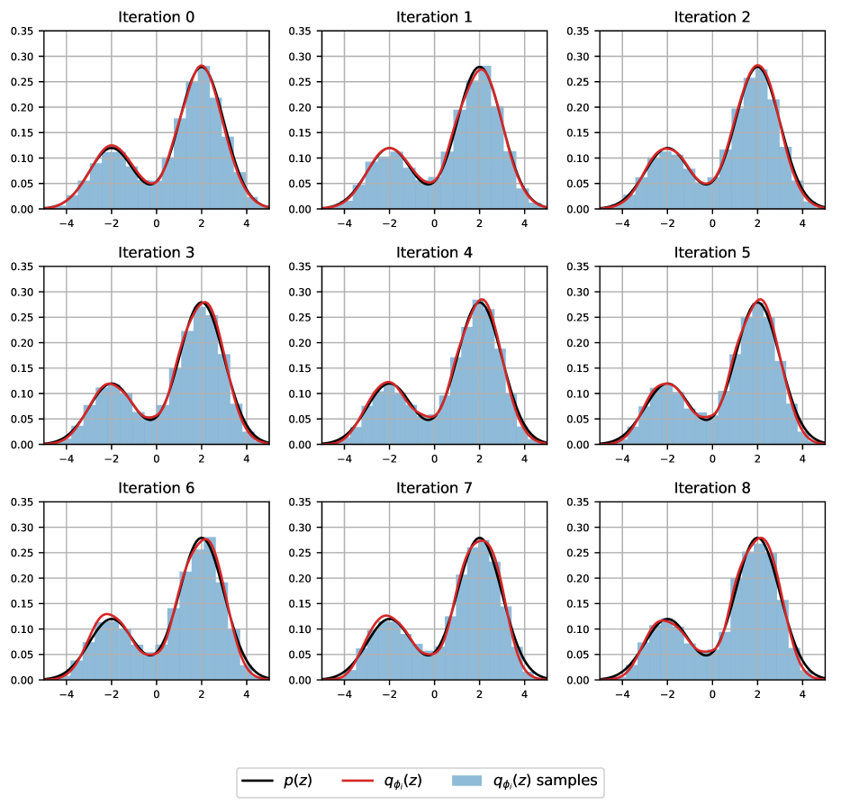
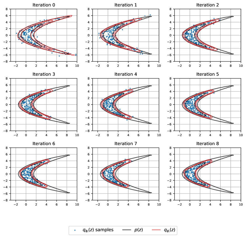
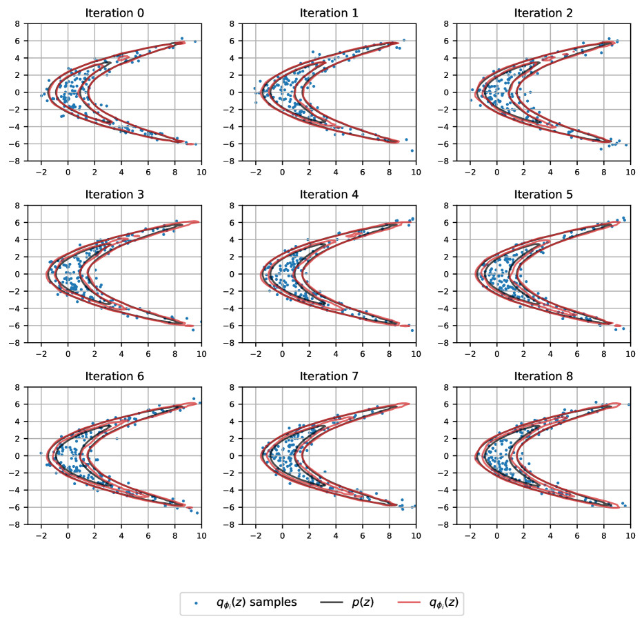
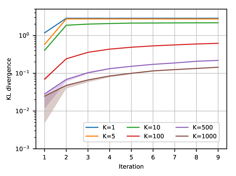
For sequential approximation toy task, we follow [40] and use the following target distributions. For one-dimensional Gaussian mixture, p(z)=0.3𝒩(z|2,1)+0.7𝒩(z| 2,1)𝑝𝑧0.3𝒩conditional𝑧210.7𝒩conditional𝑧21p(z)=0.3\mathcal{N}(z\,|\,{-2},1)+0.7\mathcal{N}(z\,|\,2,1). For the “banana” distribution, p(z1,z2)=𝒩(z1|z22/4,1)𝒩(z2| 0,4)𝑝subscript𝑧1subscript𝑧2𝒩conditionalsubscript𝑧1superscriptsubscript𝑧2241𝒩conditionalsubscript𝑧2 04p(z_{1},z_{2})=\mathcal{N}(z_{1}\,|\,z_{2}^{2}/4,1)\mathcal{N}(z_{2}\,|\,0,4).

For both target distributions, we optimize the objective using Adam optimizer with initial learning rate 102superscript10210^{-2} and decaying it by 0.50.50.5 every 500 steps. On each iteration of sequential approximation, we train for 5000 steps. We reinitialize all trainable parameters and optimizer statistics before each iteration. Before each update of the parameters, we average 200 Monte Carlo samples of the gradients. During evaluation, we used 105superscript10510^{5} Monte Carlo samples to estimate the expectations involved in the lower and upper bounds on KL divergence.
Refer to caption
Figure 5: Sequential approximation. Area is shaded between lower and upper bounds of KL(qϕi(z)p(z))KLconditionalsubscript𝑞subscriptitalic-ϕ𝑖𝑧𝑝𝑧{\mathrm{KL}}(q_{\phi_{i}}(z)\,\|\,p(z)) for different training values of K1=K2=Ksubscript𝐾1subscript𝐾2𝐾K_{1}=K_{2}=K, and the solid lines represent the corresponding upper bounds. During evaluation, K=104𝐾superscript104K=10^{4} is used. Here p(z)𝑝𝑧p(z) is a two-dimensional “banana“. Lower is better.
Refer to caption
Figure 6: Learned distributions after each iteration for Gaussian mixture target distribution, K=100𝐾100K=100 during training.
Refer to caption
Figure 7: Learned distributions after each iteration for Gaussian mixture target distribution, K=1000𝐾1000K=1000 during training.
Refer to caption
Figure 8: Learned distributions after each iteration for “banana” target distribution, K=100𝐾100K=100 during training.
Refer to caption
Figure 9: Learned distributions after each iteration for “banana” target distribution, K=1000𝐾1000K=1000 during training.