Interpretable Convolutional Neural Networks via Feedforward Design
Abstract
The model parameters of convolutional neural networks (CNNs) are determined by backpropagation (BP). In this work, we propose an interpretable feedforward (FF) design without any BP as a reference. The FF design adopts a data-centric approach. It derives network parameters of the current layer based on data statistics from the output of the previous layer in a one-pass manner. To construct convolutional layers, we develop a new signal transform, called the Saab (Subspace approximation with adjusted bias) transform. It is a variant of the principal component analysis (PCA) with an added bias vector to annihilate activation’s nonlinearity. Multiple Saab transforms in cascade yield multiple convolutional layers. As to fully-connected (FC) layers, we construct them using a cascade of multi-stage linear least squared regressors (LSRs). The classification and robustness (against adversarial attacks) performances of BP- and FF-designed CNNs applied to the MNIST and the CIFAR-10 datasets are compared. Finally, we comment on the relationship between BP and FF designs.
keywords:
Interpretable machine learning, convolutional neural networks, principal component analysis, linear least-squared regression, cross entropy, dimension reduction.1 Introduction
Convolutional neural networks (CNNs) have received a lot of attention in recent years due to their outstanding performance in numerous applications. We have also witnessed the rapid development of advanced CNN models and architectures such as the generative adversarial networks (GANs) [1], the ResNets [2] and the DenseNet [3].
A great majority of current CNN literature are application-oriented, yet efforts are made to build theoretical foundation of CNNs. Cybenko [4] and Hornik et al. [5] proved that the multi-layer perceptron (MLP) is a universal approximator in late 80s. Recent studies on CNNs include: visualization of filter responses at various layers [6, 7, 8], scattering networks [9, 10, 11], tensor analysis [12], generative modeling [13], relevance propagation [14], Taylor decomposition [15], multi-layer convolutional sparse modeling [16] and over-parameterized shallow neural network optimization [17].
More recently, CNN’s interpretability has been examined by a few researchers from various angles. Examples include interpretable knowledge representations [18], critical nodes and data routing paths identification [19], the role of nonlinear activation [20], convolutional filters as signal transforms [21, 22], etc. Despite the above-mentioned efforts, it is still challenging to provide an end-to-end analysis to the working principle of deep CNNs.
Given a CNN architecture, the determination of network parameters can be formulated as a non-convex optimization problem and solved by backpropagation (BP). Yet, since non-convex optimization of deep networks is mathematically intractable [17], a new methodology is adopted in this work to tackle the interpretability problem. That is, we propose an interpretable feedforward (FF) design without any BP and use it as a reference. The FF design adopts a data-centric approach. It derives network parameters of the current layer based on data statistics from the output of the previous layer in a one-pass manner. This complementary methodology not only offers valuable insights into CNN architectures but also enriches CNN research from the angles of linear algebra, statistics and signal processing.
To appreciate this work, a linear algebra viewpoint on machine learning is essential. An image, its class label and intermediate representations are all viewed as high-dimensional vectors residing in certain vector spaces. For example, consider the task of classifying a set of RGB color images of spatial resolution into classes. The input vectors are of dimension . Each desired output is the unit dimensional vector in a 10-dimensional (10D) space. To map samples from the input space to the output space, we conduct a sequence of vector space transformations. Each layer provides one transformation. A dimension of a vector space can have one of three meanings depending on the context: a representation unit, a feature or a class label. The term “dimension” provides a unifying framework for the three different concepts in traditional pattern recognition.
In our interpretation, each CNN layer corresponds to a vector space transformation. To take computer vision applications as an example, CNNs provide a link from the input image/video space to the output decision space. The output can be an object class (e.g., object classification), a pixel class (e.g., semantic segmentation) or a pixel value (e.g. depth estimation, single image super-resolution, etc.) The training data provide a sample distribution in the input space. We use the input data distribution to determine a proper transformation to the output space. The transformation is built upon two well-known ideas: 1) dimension reduction through subspace approximations and/or projections, and 2) training sample clustering and remapping. The former is used in convolutional layers construction (e.g., filter weights selection and max pooling) while the latter is adopted to build FC layers. They are elaborated a little more below.
The convolutional layers offer a sequence of spatial-spectral filtering operations. Spatial resolutions become coarser along this process gradually. To compensate for the loss of spatial resolution, we convert spatial representations to spectral representations by projecting pixels in a window onto a set of pre-selected spatial patterns obtained by the principal component analysis (PCA). The transformation enhances discriminability of some dimensions since a dimension with a larger receptive field has a better chance to “see” more. We develop a new transform, called the Saab (Subspace approximation with adjusted bias) transform, in which a bias vector is added to annihilate nonlinearity of the activation function. The Saab transform is a variant of PCA, and it contributes to dimension reduction.
The FC layers provide a sequence of operations that involve “sample clustering and high-to-low dimensional mapping”. Each dimension of the output space corresponds to a ground-truth label of a class. To accommodate intra-class variability, we create sub-classes of finer granularity and assign pseudo labels to sub-classes. Consider a three-level hierarchy – the feature space, the sub-class space and the class space. We construct the first FC layer from the feature space to the sub-class space using a linear least-squared regressor (LSR) guided by pseudo-labels. For the second FC layer , we treat pseudo-labels as features and conduct another LSR guided by true labels from the sub-class space to the class space. A sequence of FC layers actually corresponds to a multi-layer perceptron (MLP). To the best of our knowledge, this is the first time to construct an MLP in an FF manner using multi-stage cascaded LSRs. The FF design not only reduces dimensions of intermediate spaces but also increases discriminability of some dimensions gradually. Through transformations across multiple layers, it eventually reaches the output space with strong discriminability.
LeNet-like networks are chosen to illustrate the FF design methodology for their simplicity. Examples of LeNet-like networks include the LeNet-5 [23] and the AlexNet [24]. They are often applied to object classification problems such as recognizing handwritten digits in the MNIST dataset and 1000 object classes in the ImageNet dataset. The classification and robustness (against adversarial attacks) performances of BP- and FF-designed CNNs on the MNIST and the CIFAR-10 datasets are reported and compared. It is important to find a connection between the BP and the FF designs. To shed light on their relationship, we measure cross-entropy values at dimensions of intermediate vector spaces (or layers).
The rest of this paper is organized as follows. The related background is reviewed in Sec. 2. The FF design of convolutional layers is described in Sec. 3. The FF design of FC layers is presented in Sec. 4. Experimental results for the MNIST and the CIFAR-10 datasets are given in Sec. 5. Follow-up discussion is made in Sec. 6. Finally, concluding remarks are drawn in Sec. 7.
2 Background
2.1 Computational neuron
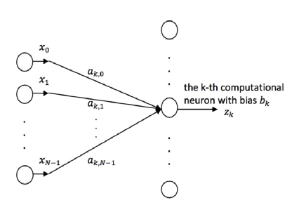
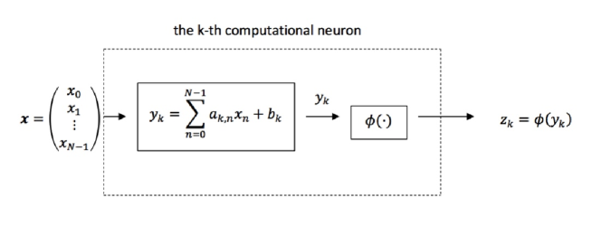
The computational neuron serves as the basic building element of CNNs. As shown in Fig. 1, it consists of two stages: 1) affine computation and 2) nonlinear activation. The input is an -dimensional random vector . The th neuron has filter weights that can be expressed in vector form as , and one bias term . The affine computation is
| (1) |
where is the filter weight vector associated with the th neuron. With the ReLU nonlinear activation function, the output after ReLU can be written as
| (2) |
In the following discussion, we assume that input is a zero-mean random vector and the set of filter weight vectors is normalized to to be with unit length (i.e. ). The filter weight vectors are adjustable in the training yet they are given and fixed in the testing. To differentiate the two situations, we call them anchor vectors in the testing case. Efforts have been made to explain the roles played by anchor vector and nonlinear activation in [20, 21, 22].
(a)
(b)
2.2 Linear space spanned by anchor vectors
It is easier to explain the role of anchor vectors by setting the bias term to zero. This constraint will be removed in Sec. 3. If , Eq. (1) reduces to . Suppose that there are anchor vectors with in a convolutional layer. One can examine the role of each anchor vector individually and all anchor vectors jointly. They lead to two different interpretations.
-
1.
A set of parallel correlators [20, 21]
If the correlation between and is weak (or strong), response will have a small (or large) magnitude. Thus, each anchor vector can be viewed as a correlator or a matched filter. We can use a set of correlators to extract pre-selected patterns from input by thresholding . These correlators can be determined by BP. In a FF design, one can apply the -means algorithm to input samples to obtain clusters and set their centroids to . -
2.
A set of unit vectors that spans a linear subspace [22]
By considering the following set of equations jointly:(3) the output vector, , is the projection of the input vector onto a subspace spanned by , . One can get an approximate to in the space spanned by anchor vectors from the projected output . With this interpretation, we can use the principal component analysis (PCA) to find a subspace and determine the anchor vector set accordingly.
The above two interpretations allow us to avoid the BP training procedure for filter weights in convolutional layers. Instead, we can derive anchor vectors from the statistics of input data. That is, we can compute the covariance matrix of input vectors and use the eigenvectors as the desired anchor vectors . This is a data-centric approach. It is different from the traditional BP approach that is built upon the optimization of a cost function defined at the system output.
2.3 Role of nonlinear activation
The need of nonlinear activation was first explained in [20]. The main result is summarized below. Consider two inputs and with the simplifying assumption:
| (4) |
The two inputs, and , are negatively correlated. For example, if is a pattern composed by three vertical stripes with the middle one in black and two side ones in white, then is also a three-vertical-stripe pattern with the middle one in white and two side ones in black. They are different patterns, yet one can be confused for the other if there is no ReLU. To show this, we first compute their corresponding outputs
| (5) | |||||
| (6) |
where and appear in the th element as shown above. Vectors and will serve as inputs to the next stage. The outgoing links from the th node can take positive or negative weights. If there is no ReLU, a node at the second layer cannot differentiate whether the input is or since the following two situations yield the same output:
-
(a)
a positive correlation () followed by a positive outgoing link from node ; and
-
(b)
a negative correlation () followed by a negative outgoing link from node .
Similarly, the following two situations will also yield the same output:
-
(a)
a positive correlation () followed by a negative outgoing link from node ; and
-
(b)
a negative correlation () followed by a positive outgoing link from node .
This is called the sign confusion problem. The ReLU operator plays the role of a rectifier that eliminates case (b). In the example, input will be blocked by the system. A trained CNN has its preference on images over their foreground/background reversed ones. A classification example conducted on the original and reversed MNIST datasets was given in [20] to illustrate this point.
To resolve the sign confusion problem, a PCA variant called the Saak transform was proposed in [22]. The Saak transform augments transform kernel with its negative , leading to transform kernels in total. Any input vector, , will have a positive/negative correlation pair with kernel pair . When a correlation is followed by ReLU, one of the two will go through while the other will be blocked. In other words, the Saak transform splits positive/negative correlations, , into positive/negative two channels. To resolve the sign confusion problem, it pays the price of doubled spectral dimensions. In the following section, we will introduce another PCA variant called the Saab (Subspace approximation with adjusted bias) transform. The Saab transform can address the sign confusion problem and avoid the spectral dimension doubling problem at the same time.
3 Feedforward design of convolutional layers
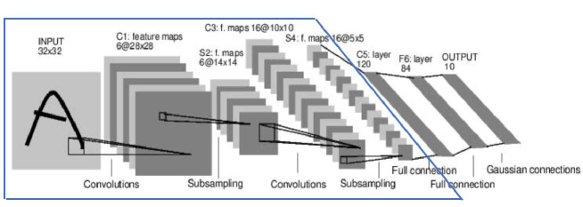
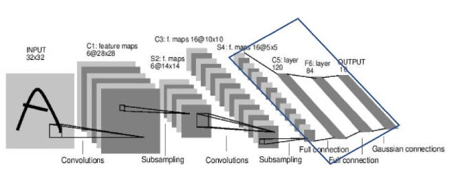
In this section, we study the construction of convolutional layers in the LeNet-5 as shown in the enclosed parallelogram in Fig. 2. We first examine the spatial-spectral filtering in Sec. 3.1. The Saab transform and its bias selection is studied in Sec. 3.2. Then, we discuss the max pooling operation in Sec. 3.3. Finally, we comment on the effect of cascaded convolutional layers in Sec. 3.4.
3.1 Spatial-spectral filtering
There is a clear distinction between representations and features in traditional image processing. Image representations are obtained by transforms such as the Fourier transform, the discrete Cosine transform and the wavelet transform, etc. Image transforms are invertible. Image features are extracted by detectors such as those for edges, textures and salient points. The distinction between image representations and image features is blurred in CNNs as mentioned in Sec. 1. An input image goes through a sequence of vector space transformations. Each dimension of intermediate spaces can be viewed as either a representation or a feature. The cascade of spatial-spectral filtering and spatial pooling at a convolutional layer provides an effective way in extracting discriminant dimensions. Without loss of generality, we use the LeNet-5 applied to the MNIST dataset as an illustrative example.
It is not a good idea to conduct pixel-wise image comparison to recognize handwritten digits since there exists a wide range of varieties in the spatial domain for the same digit. Besides, the pixel-wise comparison operation is sensitive to small translation and rotation. For example, if we shift the same handwritten digit image “1” horizontally by several pixels, the original and shifted images will have poor match in the spatial domain. A better way is to consider the neighborhood of a pixel, and find a spectral representation for the neighborhood. For example, we use a patch of size centered at a target pixel as its neighborhood. The stroke inside a patch is a 2D pattern. We can use PCA to find a set of dominant stroke patterns (called anchor vectors) to form a vector space and represent any neighborhood pattern as a linear combination of anchor vectors.
In the multi-stage design, the convolutional layers provide a sequence of spatial-spectral transformations that convert an input image to its joint spatial-spectral representations layer by layer. Spatial resolutions become lower gradually. To compensate the spatial resolution loss, we trade spatial representations for spectral representations by projecting local spatial-spectral cuboids onto PCA-based kernels. The main purpose is to enhance discriminability of some dimensions. Generally, a spatial-spectral component with a larger receptive field has a better chance to be discriminant since it can “see” more. Another advantage of the PCA-based subspace approximation is that it does not demand image labels.
One related question is whether to conduct the transform in overlapping or non-overlapping windows. Signal transforms are often conducted in non-overlapping windows for computational and storage efficiency. For example, the block discrete Cosine transform (DCT) is adopted in image/video compression. For the same reason, the Saak transform in [22] is conducted on non-overlapping windows.However, the LeNet-5 uses overlapping windows. The MNIST dataset contains gray-scale images of dimension . At the first convolutional layer, the LeNet-5 has 6 filters of size with stride equal to one. The output image cuboid has a dimension of by taking the boundary effect into account. If we ignore the boundary effect and apply spatial-spectral filtering operations at every pixel, the output data dimension is enlarged by a factor of with respect to the input. This redundant representation seems to be expensive in terms of higher computational and storage resources. However, it has one advantage. That is, it provides a richer feature set for selection. Redundancy is controlled by the stride parameter in CNN architecture specification.
3.2 Saab transform and bias selection
We repeat the affine transform in Eq. (1) below:
| (7) |
The Saab transform is nothing but a specific way in selecting anchor vector and bias term . They are elaborated in this subsection.
Anchor vectors selection. By following the treatment in [20, 21, 22], we first set and divide anchor vectors into two categories:
-
1.
DC anchor vector .
-
2.
AC anchor vectors , .
The terms “DC” and “AC” are borrowed from circuit theory, and they denote the “direct current” and the “alternating current”, respectively. Based on the two categories of anchor vectors, we decompose the input vector space, , into the direct sum of two subspaces:
| (8) |
where is the subspace spanned by the DC anchor and and is the subspace spanned by the AC anchors. They are called the DC and AC subspaces accordingly. For any vector , we can project to to get its DC component. That is, we have
| (9) |
Subspace is the orthogonal complement to in . We can express the AC component of as
| (10) |
Clearly, we have and . We conduct the PCA on all possible and, then, choose the first principal components as AC anchor vectors , .
Bias selection. Each bias term, , in Eq. (7), provides one extra degree of freedom per neuron for the end-to-end penalty minimization in the BP design. Since it plays no role in linear subspace approximation, it was ignored in [20, 21, 22]. Here, the bias term is leveraged to overcome the sign confusion problem in the Saab transform. We impose two constraints on the bias terms.
-
(B1)
Positive response constraint
We choose the th bias, , to guarantee the th response a non-negative value. Mathematically, we have(11) for all input .
-
(B2)
Constant bias constraint
We demand that all bias terms are equal; namely,(12)
Due to Constraint (B1), we have
| (13) |
That is, we have the same output with or without the ReLU operation. This simplifies our CNN analysis greatly since we remove nonlinearity introduced by the activation function. Under Constraint (B2), we only need to determine a single bias value (rather than different bias values). It makes the Saab transform design easier. Yet, there is a deeper meaning in (B2).
Let lie in the AC subspace of the input space, . We can re-write Eq. (7) in vector form as
| (14) |
where is the unit constant-element vector in the output space . The first term in Eq. (14) is zero due to the assumption. The second and third terms lie in the AC and DC subspaces of the output space, , respectively. In other words, the introduction of the constant-element bias vector has no impact on the AC subspace but the DC subspace when multiple affine transforms are in cascade. It is essential to impose (B2) so that the multi-stage Saab transforms in cascade are mathematically tractable. That is, the constant-element bias vector always lies in the DC subspace, . It is completely decoupled from and its PCA. We conduct PCA on the AC subspace, , layer by layer to obtain AC anchor vectors at each layer.
The addition of a constant-element bias vector to the transformed output vector is nothing but shift each output response by a constant amount. We derive a lower bound on this amount in the appendix. The bias selection rule can be stated below.
-
1.
Bias selection rule
All bias terms should be equal (i.e., ), and they should meet the following constraint:(15) where is an input vector and is the dimension of the output space .
3.3 Spatial pooling
Rationale of maximum pooling. Spatial pooling helps reduce computational and storage resources. However, this cannot explain a common observation: “Why maximum pooling outperforms the average pooling?” Here, we interpret the pooling as another filtering operation that preserves significant patterns and filters out insignificant ones. Fig. 3 shows four spatial locations, denoted by A, B, C, D, in a representative non-overlapping block. Suppose that filters are used to generate responses at each location. Then, we have a joint spatial-spectral response vector of dimension . Pooling is used to reduce the spatial dimension of this response vector from to so that the new response vector is of dimension . It is performed at each spectral component independently. Furthermore, all response values are non-negative due to the ReLU function.
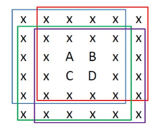
Instead of viewing convolution and pooling operations as two individual ones, we examine them as a whole. The new input is the union of the four neighborhoods, which is a patch of size . The compound operations, consisting of convolution and pooling, is to project the enlarged neighborhood patch of dimension to a subspace of dimension spanned by anchor vectors (or filters). The convolution-plus-pooling operations is equivalent to:
-
1.
Projecting a patch of size to any smaller one of size centered at locations A-D with zero padding in uncovered areas;
-
2.
Projecting the patch of size to all anchor vectors.
Each spectral component corresponds to a visual pattern. For a given pattern, we have four projected values obtained at locations A, B, C, D. By maximum pooling, we choose the maximum value among the four. That is, we search the target visual pattern in a slightly larger window (i.e. of size ) and use the maximum response value to indicate the best match within this larger window.
On the other hand, infrequent visual patterns that are less relevant to the target task will be suppressed by the compound operation of spatial-spectral filtering (i.e. the Saab transform) and pooling. The convolutional kernels of the Saab transform are derived from the PCA. The projection of these patterns on anchor vectors tend to generate small response values and they will be removed after pooling.
The same principle can be generalized to pooling in deeper layers. A spatial location in a deep layer corresponds to a receptive field in the input source image. The deeper the layer the larger the receptive field. A spectral component at a spatial location can be interpreted as a projection to a dominant visual pattern inside its receptive field. A block in a deep layer correspond to the union of four overlapping receptive fields, each of which is associated with one spatial location. To summarize, the cascade of spatial-spectral filtering and maximum pooling can capture “visually similar but spatially displaced” patterns.
3.4 Multi-layer compound filtering
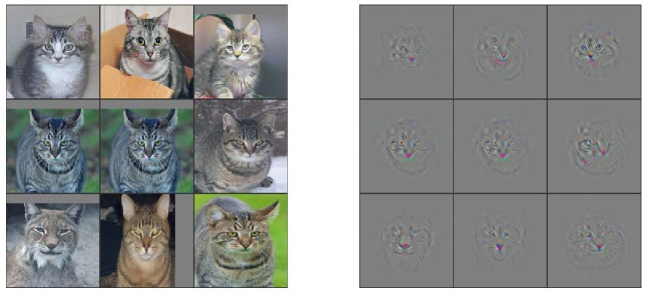
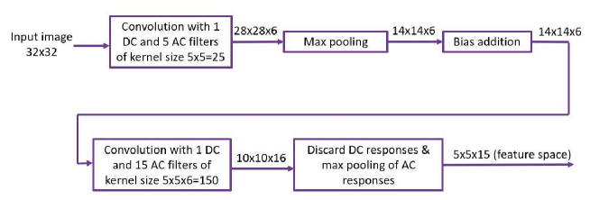
The cascade of multiple convolutional layers can generate a rich set of image patterns of various scales as object signatures. We call them compound filters. One can obtain interesting compound filters through the BP design. To give an example, we show the nine top-ranked images that have the strongest responses with respect to a certain convolutional filter (called the cat face filter) in the 5th convolutional layer of the AlexNet [24] and their corresponding filter responses in Fig. 4. We see cat face contours clearly in the right subfigure. They are of size around . The compound filtering effect is difficult to implement using a single convolutional layer (or a single-scale dictionary). In the FF design, a target pattern is typically represented as a linear combination of responses of a set of orthogonal PCA filters. These responses are signatures of the corresponding receptive field in the input image. There is no need to add the bias term in the last convolutional layer since a different design methodology is adopted for the construction of FC layers. The block-diagram of the FF design of the first two convolutional layers of the LeNet-5 is shown in Fig. 5.
4 Feedforward design of FC layers
The network architecture the LeNet-5 is shown in Fig. 6, where FC layers enclosed by a blue parallelogram. The input to the first FC layer consists of data cuboids of dimension indicated by S4 in the figure. The output layer contains 10 output nodes, which can be expressed as a 10-dimensional vector. There are two hidden layers between the input and the output of dimensions 120 and 84, respectively. We show how to construct FC layers using a sequence of label-guided linear least-squared regressors.
4.1 Least-squared regressor (LSR)
In the FF design, each FC layer is treated as a linear least-squared regressor. The output of each FC layer is a one-hot vector whose elements are all set to zero except for one element whose value is set to one. The one-hot vector is typically adopted in the output layer of CNNs. Here, we generalize the concept and use it at the output of each FC layer. There is one challenge in this generalization. That is, there is no label associated with an input vector when the output is one of the hidden layers. To address it, we conduct the k-means clustering on the input, and group them into clusters where is the number of output nodes. Then, each input has two labels – the original class label and the new cluster label. We combine the class and the cluster labels to create pseudo-labels for each input. Then, we can set up a linear least-squared regression problem using the one-hot vector defined by pseudo-labels at this layer. Then, we can conduct the label-guided linear least-squared regression in multiple stages (or multi-layers).
To derive a linear least-squared regressor, we set up a set of linear equations that relates the input and the output variables. Suppose that and are input and output vectors. That is, we have
| (16) |
where , , , are scalars to account for bias terms. After nonlinear activation, each FC layer is a rectified linear least-squared regressor.
There are three FC layers in cascade in the LeNet-5.
-
1.
First FC layer (or Stage I): and .
-
2.
Second FC layer (or Stage II): and .
-
3.
Third FC layer (or Stage III): and .
The input data to the first FC layer is a data cuboid of dimension since the DC responses are removed (or dropped out). The output data of the third FC layer is the following ten one-hot vector of dimension :
| (17) |
Each one-hot vector denotes the label of a hand-written digit. For example, we can use the above ten one-hot vector to denote digits “0”, “1”, , “9”, respectively.
By removing the two middle hidden layers of dimensions 120 and 84 and conducting the linear least-squared regression on the input feature vector of dimension 375 with 10 one-hot vectors as the desired output directly, this is nothing but traditional one-stage least-squared regression. However, its performance is not very good. The advantage of introducing hidden layers and the way to generate more pseudo-labels will be discussed below.
4.2 Pseudo-labels generation
To build least-squared regressors in Stages I and II, we need to define labels for input. Here, we consider the combination of two factors: the original label (denoted by ) and the auxiliary label (denoted by i, ii, , x, xi, xii, etc.) of an input data sample. Each input training sample has its own original label. To create its auxiliary label, we conduct the k-means clustering algorithm on training samples of the same class. For example, we can divide samples of the same digit into 12 clusters to generate 12 pseudo classes. The centroid of a class provides a representative sample for that class. The reason to generate pseudo classes is to capture the diversity of a single class with more representative samples, say, from one to twelve in the LeNet-5.
As a result, we can set up 120 linear equations to map samples in the input feature space to 120 one-hot vectors, which form the output feature space. A one-hot vector is a unit vector in an orthogonal feature space. Ideally, an LSR is constructed to map all samples in a pseudo-class to the unit vector of the target dimension and block the mapping of these samples to other unit vectors. This is difficult to achieve in practice since its performance is highly correlated with the feature distribution in the input space. If two pseudo classes have strong overlaps in the feature space (say, some 7’s and 9’s are visually similar), we expect a significant projection of samples in one pseudo class to the one-hot vector of another pseudo-class, vice versa. This is called “leakage” (with respect to the original pseudo class) or “interference” (with respect to other pseudo classes).
The output of the last convolutional layer has a physical explanation in the FF design. It is a spatial-spectral transform of an input image. It provides a feature vector for the classifier in later layers. Once it is fed to the FC layer, a mathematical model is used to align the input and output feature spaces by mapping samples from a pseudo class to one of orthogonal unit vectors that span the output feature space. The purpose of feature space alignment is to lower the cross-entropy value and produce more discriminant features. Thus, the cascade of LSRs conducted in multiple FC layers is nothing but a sequential feature space alignment procedure. In contrast, BP-designed CNNs do not have such a clear cut in roles played by the convolutional and the FC layers.
5 Experimental Results
We will show experimental results conducted on two popular datasets: the MNIST dataset111http://yann.lecun.com/exdb/mnist/ and the CIFAR-10 dataset 222https://www.cs.toronto.edu/ kriz/cifar.html. Our implementation codes are available in the GitHub website.
Network architectures. The LeNet-5 architecture targets at gray-scale images only. Since the CIFAR-10 dataset is a color image dataset, we need to modify the network architecture slightly. The parameters of the original and the modified LeNet-5 are compared in Table 1. Note that the modified LeNet-5 keeps the architecture of two convolutional layers and three FC layers, which include the last output layer. The modification is needed since the input images are color images in the CIFAR-10 dataset. We use more filters at all layers, which are chosen heuristically.
| Architecture | Original LeNet-5 | Modified LeNet-5 |
|---|---|---|
| 1st Conv Layer Kernel Size | ||
| 1st Conv Layer Kernel No. | ||
| 2nd Conv Layer Kernel Size | ||
| 2nd Conv Layer Kernel No. | ||
| 1st FC Layer Filter No. | ||
| 2nd FC Layer Filter No. | ||
| Output Node No. |
| Datasets | MNIST | CIFAR-10 |
|---|---|---|
| FF | 97.2% | 62% |
| Hybrid | 98.4% | 64% |
| BP | 99.9% | 68% |
Classification performance. The testing accuracies of the BP and the FF designs for the MNIST and the CIFAR-10 datasets are compared in Table 2. Besides, we introduce a hybrid design that adoptes the FF design in the first two convolutional layers to extract features. Then, it uses the multi-layer perceptron (MLP) the last three FC layers with a built-in BP mechanism.
By comparing the FF and the Hybrid designs, we observe the performance degradation due to a poorer decision subnet without BP optimization. We see a drop of 1.2% and 2% in classification accuracies for MNIST and CIFAR-10, respectively. Next, we can see the performance degradation primarily due to a poorer feature extraction subnet without BP optimization. We see a drop of 1.5% and 4% for MNIST and CIFAR-10, respectively. Performance degradation due to the FF design is well expected. The performance gaps between the FF and the BP designs for MNIST and CIFAR-10 are, respectively, 2.7% and 6%.
| Attacks | CNN Design | MNIST | CIFAR-10 |
| FGS | BP | 6 % | 15 % |
| FGS | FF | 56 % | 21 % |
| BIM | BP | 1 % | 12 % |
| BIM | FF | 46 % | 31 % |
| Deepfool | BP | 2 % | 15 % |
| Deepfool | FF | 96 % | 59 % |
| Attacks | CNN Design | MNIST | CIFAR-10 |
| FGS | BP | 34 % | 11 % |
| FGS | FF | 4 % | 6 % |
| BIM | BP | 57 % | 14% |
| BIM | FF | 1 % | 12 % |
| Deepfool | BP | 97 % | 68 % |
| Deepfool | FF | 2 % | 16 % |
Robustness against adversarial attacks. Adversarial attacks have been extensively examined since the pioneering study in [25]. We examine three attacks: the fast gradient sign (FGS) method [26], the basic iterative method (BIM) [27] and the Deepfool method [28].
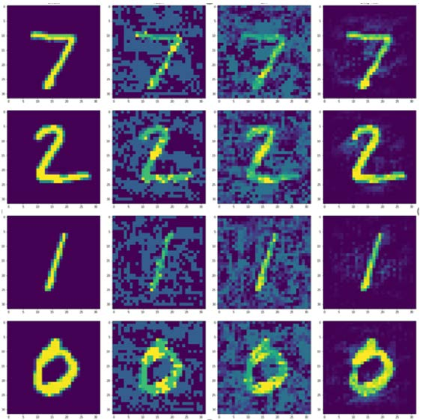
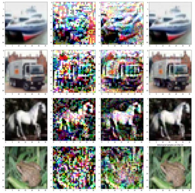
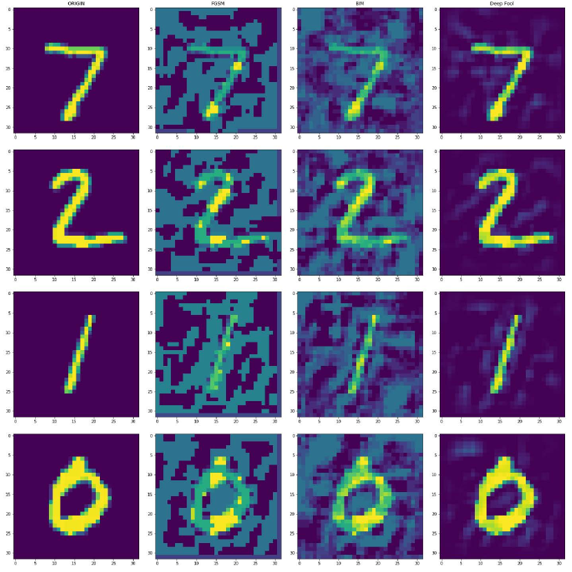
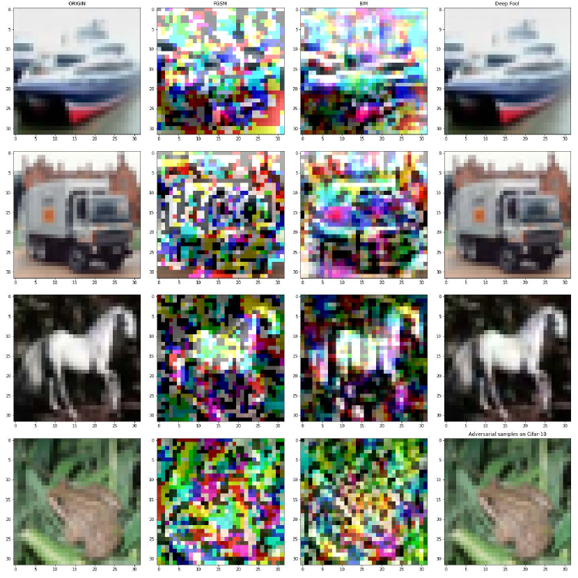
We generate adversarial attacks targeting at the BP and the FF designs individually. Exemplary attacked images targeting at BP and FF designs are shown in Fig. 8 and Fig. 9, respectively. As shown in Figs. 8 and 9, the Deepfool provides attacks of least visual distortion. The quality of the FGS- and BIM-attacked images is poor. Since one can develop algorithms to filter out poor quality images, we should be more concerned with the Deepfool attack.
The classification accuracies of BP and FF designs against attacked images are compared in Tables 3 and 4. The classification performance of BP and FF designs degrades significantly against their individual attacks. This example indicates that, once CNN model parameters are known, one can design powerful adversarial attacks to fool the recognition system yet high-quality adversarial attacks have little effect on the HVS. The fact that CNNs are vulnerable to adversarial attacks of good visual quality has little to do model parameters selection methodologies. It is rooted in the end-to-end interconnection architecture of CNNs. To mitigate catastrophic performance degradation caused by adversarial attacks, one idea is to consider multiple models as explained below.
Robustness enhancement via ensemble methods. One can generate different FF-designed CNN models using multiple initializations for the k-means clustering in the multi-stage LSR models. For example, we construct the following three FF-designed CNNs that share the same convolutional layer but different FC layers.
-
1.
FF-1: Adopt the k-means++ initialization [29] in the k-means clustering;
-
2.
FF-2: Adopt the random initialization in the k-means clustering;
-
3.
FF-3: Cluster five digits into 13 clusters and the other five digits into 11 clusters in the design of the first AC layer (with 120 output dimensions) and adopt the k-means++ initialization.
| MNIST | FF-1 | FF-2 | FF-3 |
| Deepfool attacking FF-1 | 2% | 79% | 81% |
| Deepfool attacking FF-2 | 78% | 2% | 81% |
| Deepfool attacking FF-3 | 79% | 80% | 2% |
| CIFAR-10 | FF-1 | FF-2 | FF-3 |
|---|---|---|---|
| Deepfool attacking FF-1 | 16% | 47% | 48% |
| Deepfool attacking FF-2 | 49% | 17% | 49% |
| Deepfool attacking FF-3 | 48% | 49% | 15% |
If the model parameters of the three FF designs are known, attackers can design adversarial attacks by targeting at each of them individually. The test accuracies of FF-1, FF-2 and FF-3 against the Deepfool attack for the MNIST and the CIFAR-10 datasets are given in Tables 5 and 6, respectively. We see that an adversarial attack is primarily effective against its target design. To enhance robustness, we may adopt an ensemble method by fusing their classification results (e.g., majority voting, bagging, etc.). This is a rich topic that goes beyond the scope of this work. We will report our further investigation in a separate paper. Although the ensemble method applies to both BP and FF designs, the cost of building an ensemble system of multiple FF networks is significantly lower than that of multiple BB networks.
6 Discussion
Some follow-up discussion comments are provided in this section. First, comparisons between FF and BP designs are made in Sec. 6.1. Then, further insights into the BP and FF designs are given in Sec. 6.2.
6.1 General comparison
| Design | BP | FF |
|---|---|---|
| Principle | System optimization centric | Data statistics centric |
| Math. Tools | Non-convex optimization | Linear algebra and statistics |
| Interpretability | Difficult | Easy |
| Modularity | No | Yes |
| Robustness | Low | Low |
| Ensemble Learning | Higher Complexity | Lower Complexity |
| Training Complexity | Higher | Lower |
| Architecture | End-to-end network | More flexible |
| Generalizability | Lower | Higher |
| Performance | State-of-the-art | To be further explored |
The properties of FF and BP designs are compared in various aspects in Table 7. They are elaborated below.
Principle. The BP design is centered on three factors: a set of training and testing data, a selected network architecture and a selected cost function at the output end for optimization. Once all three are decided, the BP optimization procedure is straightforward. The datasets are determined by applications. Most research contributions come from novel network architectures and new cost functions that achieve improved target performance. In contrast, the FF design exploits data statistics (i.e. the covariance matrix) to determine a sequence of spatial-spectral transformations in convolutional layers with two main purposes – discriminant dimension generation and dimension reduction. The PCA-based convolution and maximum spatial pooling can be well explained accordingly. No data labels are needed in the FF design of convolutional layers. After that, the FC layers provide sequential LSR operations to enable a multi-stage decision process. Data labels are needed in the FF design of FC layers. They are used to form clusters of data of the same class to build the LSR models. Clustering is related to the sample distribution in a high-dimensional space. It is proper to examine clustering and LSR from a statistical viewpoint.
Mathematical Tools. The BP design relies on the stochastic gradient descent technique in optimizing a pre-defined cost function. When a CNN architecture is deeper, the vanishing gradient problem tends to occur. Several advanced network architectures such as the ResNets [2] were proposed to address this issue. The mathematical tool used in this work is basically linear algebra. We expect statistics to play a significant role when our focus moves to training data collection and labeling for a certain task.
Interpretability. As stated in Sec. 1, interpretability of CNNs based on the BP design (or CNN/BP in short) was examined by researchers, e.g., [18, 19]. Although these studies do shed light on some properties of CNN/BP, a full explanation of CNN/BP is very challenging. CNNs based on the FF design (or CNN/FF in short) are mathematically transparent. Since the filter weights selection strategy in CNN/FF is different from that in CNN/BP, our understanding of CNN/FF is not entirely transferable to that of CNN/BP. However, we can still explain the benefit of the multi-layer CNN architecture. Furthermore, the connection between FF and BP designs will be built by studying cross-entropy values of intermediate layers in Sec. 6.2.
Modularity. The BP design relies on the input data and the output labels. The model parameters at each layer are influenced by the information at both ends. Intuitively speaking, the input data space has stronger influence on parameters of shallower layers while the output decision space has has stronger impact on parameters of deeper layers. Shallower and deeper layers capture low-level image features and semantic image information, respectively. The whole network design is end-to-end tightly coupled. The FF design decouples the whole network into two modules explicitly. The subnet formed by convolutional layers is the data representation (or feature extraction) module that has nothing to do with decision labels. The subnet formed by FC layers is the decision module that builds a connection between the extracted feature space and the decision label space. This decoupling strategy is in alignment with the traditional pattern recognition paradigm that decomposes a recognition system into the “feature extraction” module and the ‘classification/regression” module.
Robustness. We showed that both BP and FF designs are vulnerable to adversarial attacks in Sec. 5 when the network model is fixed and known to attackers. We provided examples to illustrate that adversarial attacks lead to catastrophic performance degradation for its target network but not others. This suggests the adoption of an ensemble method by fusing results obtained by multiple FF networks. The cost of generating multiple network models by changing the initialization schemes for the k-means clustering in the FC layers is very low. This is an interesting topic worth further investigation.
Training Complexity. The BP is an iterative optimization process. The network processes all training samples once in an epoch. Typically, it demands tens or hundreds of epochs for the network to converge. The FF design is significantly faster than the BP design based on our own experience. We do not report the complexity number here since our FF design is not optimized and the number could be misleading. Instead, we would like to say that it is possible to reduce complexity in the FF design using statistics. That is, both PCA and LSR can be conducted on a small set of training data (rather than all training data). Take the filter design of the first convolutional layer as an example. The input samples of the CIFAR-10 dataset are patches of size . We need to derive a covariance matrix of dimension to conduct the PCA. It is observed that the covariance matrix converges quickly with hundreds of training images, which is much less than 50,000 training images in the CIFAR-10 dataset. One reason is that each training image provides training patches. Furthermore, there exists an underlying correlation structure between training images and patches in the dataset. Both high dimensional covariance matrix estimation [30] and regression analysis with selected samples [31] are topics in statistics. Powerful tools developed therein can be leveraged to lower the complexity of the FF design.
Architecture. The BP design has a constraint on the network architecture; i.e. to enable end-to-end BP optimization. Although we apply the FF design to CNNs here, the FF design is generally applicable without any architectural constraint. For example, we can replace the FC layers with the random forest (RF) and the support vector machine (SVM) classifiers.
Generalizability. There is a tight coupling between the data space and the decision space in the BP design. As a result, even with the same input data space, we need to design different networks for different tasks. For example, if we want to conduct object segmentation, classification and tracking as well as scene recognition and depth estimation simultaneously for a set of video clips, we need to build multiple CNNs based on the BP design (i.e., one network for one task) since the cost function for each task is different. In contrast, all tasks can share the same convolutional layers in the FF design since they only depend on the input data space. After that, we can design different FC layers for different tasks. Furthermore, we can fuse the information obtained by various techniques conveniently in the FF design. For example, features obtained by traditional image processing techniques such as edge and salient points (e.g. SIFT features) can be easily integrated with FF-based CNN features without building larger networks that combine smaller networks to serve different purposes.
Performance. The BP design offers state-of-the-art performances for many datasets in a wide range of application domains. There might be a perception that the performance of the BP design would be difficult to beat since it adopts an end-to-end optimization process. However, this would hold under one assumption. That is, the choice of the network architecture and the cost function is extremely relevant to the desired performance metric (e.g., the mean Average Precision in the object detection problem). If this is not the case, the BP design will not guarantee the optimal performance. The FF design is still in its infancy and more work remains to be done in terms of target performance. One direction for furthermore performance boosting is to exploit ensemble learning. This is particularly suitable for the FF design since it is easier to adopt multiple classifiers after the feature extraction stage accomplished by multiple convolutional layers.
6.2 Further Insights
Degree of Freedom and Overfitting. The number of CNN parameters is often larger than that of training data. This could lead to overfitting. The random dropout scheme [32] provides an effective way to mitigate overfitting. We should point out that the number of CNN model parameters is not the same as its degree of freedom in the FF design. This is because that the FF design is a sequential process. Filter weights are determined layer by layer sequentially using PCA or LSR. Since the output from the previous layer serves as the input to the current layer, filter weights of deeper layers are dependent on those of shallower layers.
Furthermore, PCA filters are determined by the covariance matrix of the input of the current layer. They are correlated. The LeNet-5 has two convolutional layers. The inputs of the first and the second convolutional layers have a dimension of and , respectively. Thus, the covariance matrices are of dimension and , respectively. Once these two covariance matrices are estimated, we can find the corresponding PCA filters accordingly.
As to FC layers, the dimension of the linear LSR matrix is roughly equal to the product of the input vector dimension and the output vector dimension. For example, for the first FC layer of the LeNet-5, the number of parameters of its LSR model is equal to
| (18) |
where the DC channel is removed. It is less than 60,000 training images in the MNIST dataset. The parameter numbers of the second FC layer and the output layer are equal to and , respectively.
Discriminability of dimensions. To understand the differences between the BP and the FF designs, it is valuable to study the discriminant power of dimensions of various layers. The cross-entropy function provides a tool to measure the discriminability of a random variable by considering the probability distributions of two or multiple object classes in this random variable. The lower the cross entropy, the higher its discriminant power. It is often adopted as a cost function at the output of a classification system. The BP algorithm is used to lower the cross entropy of the system so as to boost its classification performance. We use the cross-entropy value to measure the discriminant power of dimensions of an intermediate space.
By definition, the cross-entropy function can be written as
| (19) |
where is the sample index, is the total number of data samples, and is the loss of the th sample in form of
| (20) |
where is the class index, is the total number of object classes, is the probability for the th sample in class and is a binary indicator ( or ). We have if it is a correct classification. Otherwise, . In practice, we only need to sum up all correct classifications in computing .
To compute the cross-entropy value in Eq. (19), we adopt the k-means clustering algorithm, partition samples in the target dimension into intervals, and use the majority voting rule to predict its label in each interval. The majority voting rule is adopted due to its simplicity. Since we have the ground-truth of all training samples, we know whether they are correctly classified. Consequently, the correct classification probability, , can be computed based on the classification results in all intervals.
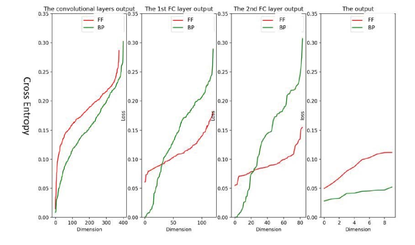
Without loss of generality, we use the LeNet-5 applied to the MNIST dataset as an example and plot rank-ordered cross-entropy values of four vector spaces in Fig. 10. They are: the output of the second convolutional layer (of dimension ), the first and the second FC layers and the output layer. The dimensions of the last three are 120, 84 and 10, respectively. We omit the plot of cross-entropy values of the first layers since each dimension corresponds to a local receptive field and their discriminant power is quite weak.
We see from Fig. 10 that the cross-entropy values of the FF design are higher than those of the BP design at the output of the 2nd convolutional layers as shown in the leftmost subfigure. This is because the FF design does not use any label information in the convolutional layer. Thus, the discriminability of dimensions (or features) of the FF design is poorer. The cross-entropy values of the FF design in the middle two subfigures are much flatter than those of the BP design. Its discriminant power is more evenly distributed among different dimensions of the first and the second FC layers. The distributions of cross-entropy values of the BP design are steeper with a larger dynamic range. The BP design has some favored dimensions, which are expected to play a significant role in inference in the BP-designed network. The cross-entropy values continue to go lower from the shallow to the deep layers, and they become the lowest at the output layer. We also see that the difference between the first and the second FC layers is not significant. Actually, the removal of the second FC layer has only a small impact to the final classification performance.
Signal representation and processing. We may use an analogy to explain the cross-entropy plots of the BP algorithm. For a given terrain specified by a random initialization seed, the BP procedure creates a narrow low-cross-entropy path that connects the input and the output spaces through iterations. Such a path is critical to the performance in the inference stage.
| Representation | BP | FF |
|---|---|---|
| Analogy | Matched Filtering | Projection onto Linear Space |
| Search | Iterative optimization | PCA and LSR |
| Sparsity | Yes | No |
| Redundancy | Yes | No |
| Orthogonality | No | Yes |
| Signal Correlation | Stronger | Weaker |
| Data Flow | Narrow-band | Broad-band |
We compare the BP and the FF designs from the signal representation and processing viewpoint in Table 8. The BP design uses an iterative optimization procedure to find a set of matched filters for objects based on the frequency of visual patterns and labels. When cat faces appear very frequently in images labeled by the cat category, the system will gradually able to extract cat face contours to represent the cat class effectively. The FF design does not leverage labels in finding object representations but conducts the PCA. As a result, it uses values projected onto the subspace formed by principal components for signal representation. The representation units are orthogonal to each other in each layer. The representation framework is neither sparse nor redundant. Being similar to the sparse representation, the BP design has a built-in dictionary. As compared to the traditional sparse representation, it has a much richer set of atoms by leveraging the cascade of multi-layer filters. The representation framework is sparse and redundant. Signal correlation is stronger in the BP design and weaker in the FF design. Finally, the representation can be viewed as narrow-band and broad-band signals in the BP and FF designs, respectively.
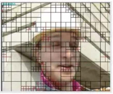
Heterogeneous spatial-spectral filtering. Although CNNs have multiple filters at a convolutional layer, they apply to all spatial locations. It is designed to capture the same pattern in different locations. However, it is not effective for large images with heterogeneous regions. As shown in Fig. 11, an image can be segmented into homogeneous regions with the HEVC coding tool [33]. Codebooks of PCA filters of different sizes can be developed in the FF design. PCA filters of the first convolutional layers describe the pixel combination rules while those of the second, third and higher convolutional layers characterize the combination rules of input spatial-spectral cuboids. The segmentation-guided FF-CNN design is natural and interesting.
7 Conclusion and Future Work
An interpretable CNN design based on the FF methodology was proposed in this work. It offers a complementary approach in CNN filter weights selection. We conducted extensive comparison between these two design methodologies. The new FF design sheds light on the traditional BP design.
As future extensions, it is worthwhile to develop an ensemble method to improve classification performance and tackle with adversarial attacks as discussed in Sec. 5. It will be interesting to provide an interpretable design for advanced CNN architectures such as ResNet, DenseNet and GANs. Furthermore, it is beneficial to introduce more statistical tools. Today’s CNN research has focused much on better and better performances for benchmark datasets with more and more complicated network architectures with respect to target applications. Yet, it is equally important to examine the setup of a CNN solution from the data viewpoint. For a given application or task, what data to collect? What data to label? How many are sufficient? Statistics is expected to play a key role in answering these questions.
The FF design methodology is still in its infancy. Our work aims at basic CNN research. It is of exploratory nature. By providing a new research and development topic with preliminary experimental results, we hope that it will inspire more follow-up work along this direction.
Appendix: Bias Selection
We use and to denote input and output flattened AC random vectors defined on 3D cuboids with two spatial dimensions and one spectral dimension. Anchor vectors, , , are the unit-length vectors obtained by the principal component analysis of and used in the Saab transform from to . We would like to add a sufficiently large bias to guarantee that all response elements are non-negative.
The correlation output between and anchor vector can be written as
| (21) |
Clearly, is in the AC subspace of since is in the AC subspace of . Let be the constant-element unit vector in . We add a constant displacement vector of length to and get a shifted output vector whose elements are
| (22) |
To ensure that is non-negative, we demand
| (23) |
The displacement length, , can be easily bound by using the following inequality:
| (24) |
Since , we have
| (25) |
By combining Eqs. (23) and (25), we obtain
| (26) |
Finally, we have the lower bound on as
| (27) |
This result is repeated in Eq. (15). Without loss of generality, we choose
| (28) |
where is a small positive number in our experiment.
Acknowledgment
This material is partially based on research sponsored by DARPA and Air Force Research Laboratory (AFRL) under agreement number FA8750-16-2-0173. The U.S. Government is authorized to reproduce and distribute reprints for Governmental purposes notwithstanding any copyright notation thereon. The views and conclusions contained herein are those of the authors and should not be interpreted as necessarily representing the official policies or endorsements, either expressed or implied, of DARPA and Air Force Research Laboratory (AFRL) or the U.S. Government. The authors would also like to give thanks to Dr. Pascal Frossard and Dr. Mauro Barni for their valuable comments to the draft of this work.
References
- [1] I. Goodfellow, J. Pouget-Abadie, M. Mirza, B. Xu, D. Warde-Farley, S. Ozair, A. Courville, Y. Bengio, Generative adversarial nets, in: Advances in neural information processing systems, 2014, pp. 2672–2680.
- [2] K. He, X. Zhang, S. Ren, J. Sun, Deep residual learning for image recognition, in: The IEEE Conference on Computer Vision and Pattern Recognition (CVPR), 2016.
- [3] G. Huang, Z. Liu, K. Q. Weinberger, L. van der Maaten, Densely connected convolutional networks, in: Proceedings of the IEEE conference on computer vision and pattern recognition, 2017.
- [4] G. Cybenko, Approximation by superpositions of a sigmoidal function, Mathematics of Control, Signals and Systems 2 (4) (1989) 303–314.
- [5] K. Hornik, M. Stinchcombe, H. White, Multilayer feedforward networks are universal approximators, Neural Networks 2 (5) (1989) 359–366.
- [6] K. Simonyan, A. Vedaldi, A. Zisserman, Deep inside convolutional networks: visualising image classification models and saliency maps, arXiv preprint arXiv:1312.6034.
- [7] M. D. Zeiler, R. Fergus, Visualizing and understanding convolutional networks, in: European Conference on Computer Vision, Springer, 2014, pp. 818–833.
- [8] B. Zhou, A. Khosla, A. Lapedriza, A. Oliva, A. Torralba, Object detectors emerge in deep scene CNNs, arXiv preprint arXiv:1412.6856.
- [9] S. Mallat, Group invariant scattering, Communications on Pure and Applied Mathematics 65 (10) (2012) 1331–1398.
- [10] J. Bruna, S. Mallat, Invariant scattering convolution networks, IEEE transactions on pattern analysis and machine intelligence 35 (8) (2013) 1872–1886.
- [11] T. Wiatowski, H. Bölcskei, A mathematical theory of deep convolutional neural networks for feature extraction, arXiv preprint arXiv:1512.06293.
- [12] N. Cohen, O. Sharir, A. Shashua, On the expressive power of deep learning: a tensor analysis, arXiv preprint arXiv:1509.05009 556.
- [13] J. Dai, Y. Lu, Y.-N. Wu, Generative modeling of convolutional neural networks, arXiv preprint arXiv:1412.6296.
- [14] S. Bach, A. Binder, G. Montavon, F. Klauschen, K.-R. Müller, W. Samek, On pixel-wise explanations for non-linear classifier decisions by layer-wise relevance propagation, PloS one 10 (7) (2015) e0130140.
- [15] G. Montavon, S. Bach, A. Binder, W. Samek, K.-R. Müller, Explaining nonlinear classification decisions with deep Taylor decomposition, arXiv preprint arXiv:1512.02479.
- [16] J. Sulam, V. Papyan, Y. Romano, M. Elad, Multi-layer convolutional sparse modeling: Pursuit and dictionary learning, arXiv preprint arXiv:1708.08705.
- [17] M. Soltanolkotabi, A. Javanmard, J. D. Lee, Theoretical insights into the optimization landscape of over-parameterized shallow neural networks, IEEE Transactions on Information Theory.
- [18] Q. Zhang, Y. Nian Wu, S.-C. Zhu, Interpretable convolutional neural networks, arXiv preprint arXiv:1710.00935.
- [19] Y. Wang, H. Su, B. Zhang, X. Hu, Interpret neural networks by identifying critical data routing paths, in: Proceedings of the IEEE Conference on Computer Vision and Pattern Recognition, 2018, pp. 8906–8914.
- [20] C.-C. J. Kuo, Understanding convolutional neural networks with a mathematical model, Journal of Visual Communication and Image Representation 41 (2016) 406–413.
- [21] C.-C. J. Kuo, The CNN as a guided multilayer RECOS transform [lecture notes], IEEE Signal Processing Magazine 34 (3) (2017) 81–89.
- [22] C.-C. J. Kuo, Y. Chen, On data-driven Saak transform, Journal of Visual Communication and Image Representation 50 (2018) 237–246.
- [23] Y. LeCun, L. Bottou, Y. Bengio, P. Haffner, Gradient-based learning applied to document recognition, Proc. IEEE 86 (11) (1998) 2278–2324.
- [24] A. Krizhevsky, I. Sutskever, G. E. Hinton, Imagenet classification with deep convolutional neural networks, in: F. Pereira, C. J. C. Burges, L. Bottou, K. Q. Weinberger (Eds.), Advances in Neural Information Processing Systems 25, Curran Associates, Inc., 2012, pp. 1097–1105.
- [25] C. Szegedy, W. Zaremba, I. Sutskever, J. Bruna, D. Erhan, I. Goodfellow, R. Fergus, Intriguing properties of neural networks, arXiv preprint arXiv:1312.6199.
- [26] I. J. Goodfellow, J. Shlens, C. Szegedy, Explaining and harnessing adversarial examples, arXiv preprint arXiv:1412.6572.
- [27] A. Kurakin, I. Goodfellow, S. Bengio, Adversarial examples in the physical world, arXiv preprint arXiv:1607.02533.
- [28] S.-M. Moosavi-Dezfooli, A. Fawzi, P. Frossard, Deepfool: a simple and accurate method to fool deep neural networks, in: Proceedings of the IEEE Conference on Computer Vision and Pattern Recognition, 2016, pp. 2574–2582.
- [29] D. Arthur, S. Vassilvitskii, k-means++: The advantages of careful seeding, in: Proceedings of the eighteenth annual ACM-SIAM symposium on Discrete algorithms, Society for Industrial and Applied Mathematics, 2007, pp. 1027–1035.
- [30] J. Fan, Y. Fan, J. Lv, High dimensional covariance matrix estimation using a factor model, Journal of Econometrics 147 (1) (2008) 186–197.
- [31] A. C. Cameron, P. K. Trivedi, Regression analysis of count data, Vol. 53, Cambridge university press, 2013.
-
[32]
N. Srivastava, G. Hinton, A. Krizhevsky, I. Sutskever, R. Salakhutdinov,
Dropout: A simple way to
prevent neural networks from overfitting, Journal of Machine Learning
Research 15 (2014) 1929–1958.
URL http://jmlr.org/papers/v15/srivastava14a.html - [33] G. J. Sullivan, J.-R. Ohm, W.-J. Han, T. Wiegand, et al., Overview of the high efficiency video coding(hevc) standard, IEEE Transactions on circuits and systems for video technology 22 (12) (2012) 1649–1668.