Classical benchmarking of Gaussian Boson Sampling on the Titan supercomputer

Abstract

Gaussian Boson Sampling is a model of photonic quantum computing where single-mode squeezed states are sent through linear-optical interferometers and measured using single-photon detectors. In this work, we employ a recent exact sampling algorithm for GBS with threshold detectors to perform classical simulations on the Titan supercomputer. We determine the time and memory resources as well as the amount of computational nodes required to produce samples for different numbers of modes and detector clicks. It is possible to simulate a system with 800 optical modes postselected on outputs with 20 detector clicks, producing a single sample in roughly two hours using $40\%$ of the available nodes of Titan. Additionally, we benchmark the performance of GBS when applied to dense subgraph identification, even in the presence of photon loss. We perform sampling for several graphs containing as many as 200 vertices. Our findings indicate that large losses can be tolerated and that the use of threshold detectors is preferable over using photon-number-resolving detectors postselected on collision-free outputs.

I Introduction

The first generation of programmable quantum devices is emerging. This has led to an increased interest to understand their practical applications and their potential to surpass the capabilities of traditional computers preskill2018quantum ; harrow2017quantum . Classical simulation algorithms play an important role in this development: they can be used to benchmark the correctness of quantum algorithms and to set the bar of performance for quantum computers pednault2017breaking ; chen201864 ; zulehner2018advanced ; biamonte2018quantum ; chen2018classical .

In photonic quantum computing, boson sampling is a sub-universal model where indistinguishable single photons are sent through linear optics interferometers and their output ports are recorded using single-photon detectors aaronson2011computational ; spring2012boson ; broome2013photonic ; tillmann2013experimental . Despite its conceptual simplicity, it is believed that simulating the behavior of a boson sampling device requires exponential time on a classical computer aaronson2011computational ; aaronson2013bosonsampling . This standard boson sampling model requires single-photon sources, which are challenging to realize experimentally at a large scale. Consequently, other variants of boson sampling have been proposed where the inputs are squeezed states, which are more amenable to implement in practice. Examples of these models include scattershot boson sampling lund2014boson ; bentivegna2015experimental ; latmiral2016towards and Gaussian Boson Sampling (GBS) hamilton2017gaussian ; kruse2018detailed . Notably, it has been shown that GBS has applications in quantum chemistry huh2015boson ; clements2017experimental ; sparrow2018simulating , optimization arrazola2018using ; arrazola2018quantum , and graph theory bradler2017gaussian .

Alongside these theoretical and experimental developments, significant progress has been made in designing classical algorithms for simulating boson sampling. In Ref. neville2017classical , a Markov chain Monte Carlo algorithm for approximate boson sampling was introduced, capable of significantly outperforming strategies based on a brute force calculation of the probability distribution. This result was improved in Ref. clifford2018classical , where an exact boson sampling algorithm was proposed having the same asymptotic complexity as the algorithm of Ref. neville2017classical , but lower runtime for fixed problem sizes.

Both of these algorithms rely on special properties of the matrix permanent, which characterizes the probability distribution of standard boson sampling with single-photon inputs. These algorithms have not been extended to other boson sampling models, whose probability distributions are described by different matrix functions. Instead, Ref. quesada2018gaussian introduced a physically-motivated and exact classical algorithm for GBS with threshold detectors. These are detectors that register a click when one or more photons are observed, but are incapable of resolving photon number. The GBS distribution with threshold detectors approximates conventional GBS with photon-number-resolving detectors when the probability of more than one photon reaching a given port is small, i.e., so that samples are collision free.

In this work, we employ the classical algorithm of Ref. quesada2018gaussian to perform classical simulation of GBS with threshold detectors. We determine the time and memory resources as well as the amount of computational nodes required to produce samples for different numbers of optical modes and detector clicks. The computational resources required to implement the algorithm increase exponentially with the number of detector clicks and polynomially with the number of modes. Therefore, for large system sizes, the simulation becomes intractable for traditional desktop computers. For such simulations, we employ the Titan supercomputer housed at Oak Ridge National Laboratories. We employ distributed memory parallelization using the message passing interface (MPI) protocol together with OpenMP multi-threading for increased performance, thus fully exploiting the capabilities of the supercomputer. This allows us to push the limits of a full simulation of GBS for a system of 800 modes, postselecting on outcomes with 20 detector clicks using 240,000 CPU cores, producing a single sample in roughly two hours.

Additionally, we employ our simulations to study the performance of a recently proposed method of using GBS for dense subgraph identification (arrazola2018using, ). We first study a small graph of 30 vertices with a planted densest subgraph of 10 vertices. Our simulation results show that using threshold detectors significantly increases the performance compared to photon-number-resolving detectors that are postselected on collision-free samples. This indicates that threshold detectors, besides being experimentally appealing due to their low cost and room-temperature operation, can lead to better results for specific applications. We also simulate sampling from this graph in the presence of photon loss. We find that significant improvement compared to classical sampling remains even in the presence of losses as large as 6 dB. Finally, we use our simulations to find dense subgraphs of a graph of 200 nodes from the DIMACS dataset johnson1996cliques .

The paper is organized as follows. In section II, we briefly review the algorithm introduced in Ref. quesada2018gaussian for GBS with threshold detectors. In section III, we analyze the memory and runtime requirements of the algorithm and discuss the benchmarking results using the Titan supercomputer to produce samples of various system sizes. In section IV, we employ the simulations for dense subgraph identification. We conclude with a discussion of our results in section V.

II The Algorithm

In this section, we detail the classical algorithm introduced in Ref. quesada2018gaussian to simulate GBS with threshold detectors. Consider a GBS device with $\ell$ modes. The main idea of the algorithm is that, even though the positive-operator valued measure (POVM) element representing a click is non-Gaussian, it can be written as the difference of two Gaussian operators. Thus, whenever the POVM element corresponding to a click is applied to a Gaussian state, it is possible to represent the conditional state of the remaining modes as the difference of two Gaussian states. Given the linearity of the action of the measurements on a quantum state, the aforementioned result generalizes to a linear combination of several Gaussian states when more clicks are detected.

Before presenting the algorithm in detail, we introduce useful notation related to Gaussian states. An $\ell$-mode Gaussian state is uniquely characterized by a $2\ell\times 2\ell$ covariance matrix $\bm{V}$ and a vector of means $\bm{\bar{r}}$. These quantities are defined as the following expectation values on the Gaussian state $\rho$:

$$\bm{V}_{ij} =\frac{1}{2}\langle\Delta\hat{r}_{i}\Delta\hat{r}_{j}+\Delta\hat{r}_{i}\Delta\hat{r}_{j}\rangle_{\rho},$$ (1a)

$$\Delta\hat{\bm{r}} =\hat{\bm{r}}-\bar{\bm{r}},$$ (1b)

$$\bar{\bm{r}} =\langle\hat{\bm{r}}\rangle_{\rho}=\text{Tr}\left(\hat{\bm{r}}\rho\right),$$ (1c)

$$\bm{\hat{r}} =(\hat{x}_{1},\hat{p}_{1},\ldots,\hat{x}_{\ell},\hat{p}_{\ell})^{T}~{},$$ (1d)

where $\hat{x}_{j}$ and $\hat{p}_{k}$ are the canonical quadratures of the modes satisfying the commutation relation $[\hat{x}_{j},\hat{p}_{k}]=2i\delta_{j,k}$, where we have set $\hbar=2$. Having set up the notation for covariance matrices, we write $\rho(\bm{V},\bm{\bar{r}})$ to identify the Gaussian state with covariance matrix $\bm{V}$ and vector of means $\bm{\bar{r}}$.

The algorithm is based on a sequence of measurements on the output ports of the device. Each time a mode is measured, the new state is computed via the following update rule. Upon measuring the $\ell^{\text{th}}$ mode of an $\ell$-mode state that is a linear combination of $M$ Gaussian states, we obtain an $\ell-1$ mode state. If a click is recorded, the new state can be expressed as a linear combination of $2M$ Gaussian states. If no click is recorded, it is a linear combination of $M$ Gaussian states. Thus, each click gives rise to a doubling of the number of states that must be recorded. Sequential measurements on all modes then gives a string of click events, namely a measurement sample. More precisely, the update rule proceeds as follows:

• Input: an $\ell$-mode state

  $$\rho_{\ell}={\sum_{k=1}^{M}}a_{k}\rho_{\ell,k}(\bm{V}_{k},\bm{\bar{r}}_{k}),$$ (2)

  that is a linear combination of Gaussian states $\rho_{\ell,k}(\bm{V}_{k},\bm{\bar{r}}_{k})$.

• For each element of the linear combination $k$, decompose the covariance matrix as

  $$\bm{V}_{k} {\to}\begin{bmatrix}\noindent\bm{V}_{A,k}&\bm{V}_{AB,k}\\ \bm{V}_{AB,k}^{T}&\bm{V}_{B,k}\end{bmatrix},\ \bm{\bar{r}}_{k}\to\begin{bmatrix}\bm{\bar{r}}_{A,k}\\ \bm{\bar{r}}_{B,k}\end{bmatrix},$$ (3)

  where $\bm{V}_{A,k}$ is a $2(\ell-1)\times 2(\ell-1)$ matrix describing modes 1 to $\ell-1$ and $\bm{V}_{AB,k}$ is a $2(\ell-1)\times 2$ matrix describing the correlations between modes 1 to $\ell-1$ and mode $\ell$. Finally, $\bm{V}_{B,k}$ is a $2\times 2$ matrix describing mode $\ell$, the mode being measured.

• Calculate the update rules for the case where no click is detected

  $$\bm{V}_{A,k}^{\prime} \to\bm{V}_{A,k}-\bm{V}_{AB,k}(\bm{V}_{B,k}+\operatorname{\mathbbm{1}}_{2})^{-1}\bm{V}_{AB,k}^{T},$$ (4a)

  $$\bm{\bar{r}}_{A,k}^{\prime} \to\bm{\bar{r}}_{A,k}-\bm{V}_{AB,k}(\bm{V}_{B,k}+\operatorname{\mathbbm{1}}_{2})^{-1}\bm{\bar{r}}_{B,k}.$$ (4b)

• Calculate the click probability:

  $$p=\sum_{k=1}^{M}a_{k}q_{k},\text{ with }q_{k}=\frac{2e^{-\bm{\bar{r}}_{B,k}^{T}(\bm{V}_{B,k}+\operatorname{\mathbbm{1}}_{2})^{-1}\bm{\bar{r}}_{B,k}}}{\sqrt{\text{det}\left(\bm{V}_{B,k}+\operatorname{\mathbbm{1}}_{2}\right)}}.$$ (5)

• Flip a coin with bias $p$

• If a click is obtained, then

  $$\rho_{\ell-1}\to \sum_{k=1}^{M}a_{k}\frac{\rho_{\ell-1,k}(\bm{V}_{A,k},\bm{\bar{r}_{A,k}})-q_{k}\rho_{\ell-1,k}(\bm{V}_{A,k}^{\prime},\bm{\bar{r}}_{A,k}^{\prime})}{1-p}$$ (6)

  otherwise

  $$\rho_{\ell-1}\to\sum_{k=1}^{M}\left(\frac{a_{k}q_{k}}{p}\right)\rho_{\ell-1,k}(\bm{V}_{A,k}^{\prime},\bm{\bar{r}}{A,k}^{\prime}).$$ (7)

• At the end of this update rule, we end up with an $\ell-1$ mode state. If no click is recorded, the state is described as a linear combination of $M$ Gaussian states. If a click is recorded, the $\ell-1$-mode state is described using $2M$ Gaussian states.

If the initial state is just a Gaussian state then $M=1$. As the algorithm progresses and $m$ clicks are detected, $2^{m}$ Gaussian states are required to describe the conditional state since each click doubles the number of Gaussian states in the linear combination. As shown in Ref. quesada2018gaussian , when $m$ clicks are detected, the complexity of the algorithm is $O(\ell^{2}2^{m})$ for a system of $\ell$ modes. Thus, this algorithm is best suited to simulating settings involving a large number of modes and comparatively few detector clicks.

III Benchmarking

Figure 1: Memory (left panel) and Titan compute nodes (right panel) required to generate a sample, plotted with respect to the number of steps $k$ in the algorithm for a device with $\ell=800$ modes and $m=20$ clicks. Each curve corresponds to a different random sample and jumps in each curve mark a click. Typically $10^{3}-10^{4}$ GB of memory and $10^{2}-10^{4}$ Titan compute nodes are needed to simulate samples with 20 clicks in a device with 800 modes.

Before discussing the numerical implementation of the algorithm, we estimate the associated computational resource requirements. Recall that the algorithm is based on sequential measurements, each one yielding a new conditional state for a subsequent measurement. Therefore, advancing to the next step requires storing the covariance matrix and the mean vector associated to the updated conditional state as well as evaluating the probability of click in the next measurement. Since the number of Gaussian states required to represent this conditional state increases exponentially with the number of clicks observed, the memory to store them and compute time to evaluate their sum also scales exponentially.

All numerical computations discussed in this paper are performed using the Titan supercomputer housed at the Oak Ridge National Laboratory. Titan is equipped with 18,688 compute nodes, each having 16 CPU cores and 32 gigabytes of memory. Hence with a total of 299,008 CPU cores and 598,016 gigabytes of memory it has a 27 petaFLOPS of theoretical peak performance titan . In the following we discuss the memory and runtime requirements for the algorithm.

Figure 2: Histogram of walltimes (left panel) and average CPU hours (right panel) to simulate samples with various number of clicks $m$ and modes $\ell=2m^{2}$. As shown in the left panel the walltime for a given number of clicks can vary depending on when the clicks are observed during the execution of the algorithms. If more clicks are observed earlier in the process, the walltime is higher. The average CPU hours, as shown in the right panel increases exponentially. Therefore, the algorithm discussed in this paper becomes intractable, even with supercomputers, for click sizes around $m=25$ when $\ell=2m^{2}$.

III.1 Memory

Consider an $\ell$-mode Gaussian initial state with covariance matrix $V$ of size $2\ell\times 2\ell$. For benchmarking purposes, we consider input states with 8 dB of squeezing and a linear optical network described by unitaries drawn from the Haar measure. For concreteness, we start the measurement at the $\ell$-th mode. After measurement of this mode, we obtain the conditional state of the remaining $\ell-1$ modes for the next measurement. If no click is observed, the conditional state remains Gaussian for the remaining modes with an updated covariance matrix of size $2(\ell-1)\times 2(\ell-1)$. On the other hand, if a click is observed, the conditional state for the remaining modes is given by a linear combination of two separate Gaussian states with covariance matrices of sizes $2(\ell-1)\times 2(\ell-1)$. Hence, each time a click is observed in the sequence of measurements, the number of covariance matrices needed to characterize the conditional state doubles. After $m$ clicks have been recorded at the $k$-th step, the state for the next step will be given by $2^{m}$ covariance matrices, each of size $2(\ell-k)\times 2(\ell-k)$. At this stage we need to store as many as $4(\ell-k)^{2}\times 2^{m}$ matrix elements to represent the state. Furthermore, numerical simulations show that to obtain an accurate estimate of the probabilities, it is necessary to work with quad precision, which requires 16 bytes of memory to store one floating point number. Therefore, the total memory (in gigabytes) to store the covariance matrices corresponding to the state at the $k$-th step is:

$$\mathbb{M}_{k}(m) =\eta\times 4(\ell-k)^{2}\times 2^{m}\times 16/2^{30}~{}~{}{\rm gigabytes}$$

$$=\eta~{}2^{m-24}(\ell-k)^{2}~{}~{}{\rm gigabytes},$$ (8)

where $\eta\approx 2$ is an overhead factor introduced to account for the temporary variables created during the execution of the algorithm.

Eq. (III.1) dictates that the memory requirement increases exponentially with $m$. For large enough $m$ and $\ell$, a local desktop computer is not sufficient to run the algorithm, since a large memory capacity is required. In order to overcome this issue, we use a distributed memory parallel implementation of the algorithm where covariance matrices are allocated over multiple compute nodes of a supercomputer (or a compute cluster). The evaluation of the sum in Eq. (5) is distributed over multiple compute nodes where each one performs a partial sum. Subsequently, at each step of the algorithm we accumulate different partial sums using the message passing interface (MPI) protocol. In addition, we employ OpenMP multithreading for enhanced speed in evaluating the partial sum at each node. Hence, the required computational resources in terms of number of compute nodes is decided by the memory requirement of the problem and the available memory at each node of the cluster. If each compute node has $\mu$ gigabytes of memory, the number $N$ of compute nodes required is at least

$$N=\frac{\mathbb{M}_{k}}{\mu},$$ (9)

where $\mathbb{M}_{k}$ is the memory needed at step $k$ during the computation. Each compute node of the Titan supercomputer has memory of $\mu=32$ gigabytes and 16 cores.

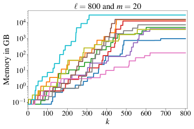
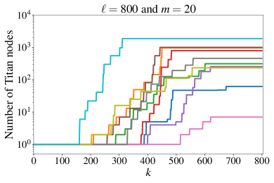
Let us consider a GBS device with 800 modes. Figure 1 shows the memory and number of Titan nodes $N$ used as we progress through different steps of the algorithm. We consider 10 different random samples with 20 clicks in each sample. Each time a click is observed, the number of covariance matrices double and so does the memory needed to store them. This is marked by jumps in each curve. A total of roughly $10^{4}-10^{5}$ GB of memory and $10^{3}-10^{4}$ nodes, each with 16 processors, are needed to generate a typical sample with 20 clicks in an 800-mode device.

It is noteworthy that the memory requirements are higher for samples in which more clicks appear in earlier steps of the algorithm. Therefore, for a sample of $m$ clicks, the memory requirement would be highest if all clicks appear in the first $m$ steps. Consider the following two scenarios for a system of $\ell$ modes: (i) all $m$ clicks are observed in the last $m$ modes, and (ii) all $m$ clicks are observed in the first $m$ modes. In the former situation, because no doubling of the number of covariance matrices occurs for the first $\ell-m$ modes, we only need to store a single covariance matrix at each step. Moreover, since the size of this matrix is equal to the number of remaining modes, it decreases with each measurement. Once clicks are detected, the number of covariance matrices increases exponentially, but they are small in size. Conversely, in the latter case, after measuring the first $m$ modes we already need to deal with an exponential number of large covariance matrices, which requires significantly more memory.

III.2 Runtime

Figure 3: Requirements for memory and appropriate number of Titan nodes (left panel) as well as associated CPU hours and walltimes for various values of $m$ (right panel), with $\ell=2m^{2}$, for extreme samples where all the clicks appear in the first $m$ of $\ell$ steps of the algorithm. It is evident from the left panel that in order to meet the memory requirements of the simulations, an increasingly large number of Titan nodes are required for larger $m$, i.e., they both scale exponentially with $m$. The total associated CPU hours (blue diamond curve in the right panel) also scales exponentially. Using the appropriate numbers of Titan nodes, the large simulations (with $m>12$) can be carried out in walltime of approximately two hours. Note that there are 18,688 compute nodes available on Titan supercomputer which can simulate these extreme samples of up to $m=22$ with $\ell=2m^{2}$.

The runtime of the algorithm is dominated by the requirement to access and process the covariance matrices stored in memory during the execution of the algorithm. Thus, runtime also scales exponentially with the number of clicks, with variations around the average runtime arising from whether most clicks are detected early or late in the algorithm. For benchmarking purposes, we fix the output in advance to have the desired number of clicks. From the perspective of the algorithm, this means that instead of flipping a coin with bias $p$ as in Eq. (5), we set the outcome of this coin flip beforehand to a desired value. This allows us to more efficiently study the properties of the algorithm without the need to wait until a sample of the desired click size is randomly obtained.

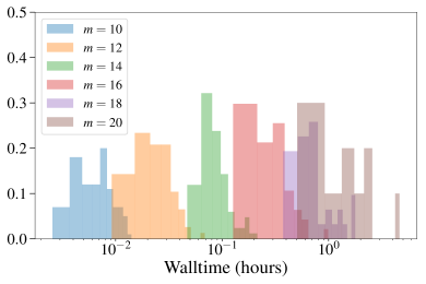
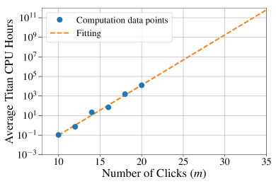
Fig. 2 shows histograms of walltimes (real user time between start and end of the simulation) to obtain a sample of various numbers of clicks $m$. Here the position of the clicks was chosen uniformly at random. For each value of $m$, there is a distribution of walltimes: higher walltimes correspond to the cases for which most of the clicks are observed earlier in the execution of the algorithm. The right panel of Fig. 2 shows the average CPU hours as a function of number of clicks $m$. It is evident that on average the CPU hours scale exponentially. A fit to these runtimes indicate that simulations of samples with $m=30$ require $10^{9}$ CPU hours, which is equivalent to the entire Titan supercomputer running for approximately five months, assuming the availability of sufficient memory.

III.3 Worst-case setting

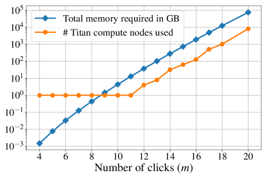
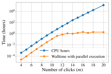
We now consider the memory and runtime requirements in the worst-case scenario of all $m$ clicks appearing in the first $m$ modes. Fig. 3 shows the computing resources needed to generate samples with different values of $m$, with $\ell=2m^{2}$. Tables 1 and LABEL:tab:run provide supporting numbers. Note that $\ell=2m^{2}$ is the regime of small collision probability aaronson2011computational , where the effect of threshold detectors is minor compared to photon-number-resolving detectors quesada2018gaussian . The left panel shows the memory and Titan nodes used for the simulations and the right panel shows the CPU hours and the walltime when appropriate number of compute nodes are utilized for parallel execution of the algorithm.

Table 1: Maximum memory needed to simulate one GBS sample for different number of modes $\ell$ and clicks $m$, where we fix $\ell=2m^{2}$.

$\ell$	$m$	Memory (GB)
50	5	0.008
200	10	4.407
450	15	739.16
800	20	76050

Table 2: Maximum runtime to simulate one sample for a device with $\ell=2m^{2}$.

$\ell$	$m$	Titan nodes	CPU hours	Walltime (hours)
200	10	1	1.81	0.11
288	12	4	21.86	0.68
392	14	32	250.17	0.97
512	16	128	2,028.91	1.98
624	18	1024	15,612.79	1.90
800	20	8192	239,773.95	1.83

It is evident from the left panel that in order to meet the memory requirements of the simulations, an exponentially large number of compute nodes are needed. The walltime for running the algorithm can be brought down to approximately two hours by using the appropriate number of compute nodes. For $m=20$ and $\ell=800$, a total of 8192 Titan nodes (131,072 processors) were employed – which is approximately 40% of the available CPUs on Titan – running for two hours. Hence, a total of 240,000 CPU hours and approximately 100,000 gigabytes of memory were consumed (see Table LABEL:tab:run). Therefore, a simulation of this algorithm with $m>22$ and $\ell=2m^{2}$ would be beyond the current capabilities the Titan supercomputer.

In the following section, we use the algorithm to generate samples for manageable problem sizes and study the application of these samples to dense subgraph identification.

IV Application: Dense subgraph identification

We study an NP-Hard optimization task known as the densest $k$-subgraph problem: given a graph $G$ with $n$ vertices, find the subgraph of size $k<n$ with the largest number of edges feige2001dense . This problem has a connection to clustering tasks that aim at finding highly correlated subsets of data, with applications in a wide range of fields such as as data mining kumar1999trawling ; angel2012dense ; beutel2013copycatch ; chen2012dense , bioinformatics fratkin2006motifcut ; saha2010dense , and finance arora2011computational .

It was shown in Refs. arrazola2018using ; arrazola2018quantum that GBS can be employed to enhance classical algorithms for the densest $k$-subgraph problem. The main insight of this approach is that, using the encoding technique of Ref. bradler2017gaussian , a GBS device can be configured to sample subgraphs in such a way that the probability of observing each subgraph is directly correlated with its density. This leads to a sampling device that selects dense subgraphs with high probability, thus aiding in their identification. In this setting, the number of modes is equal to the number of vertices in the graph and subgraphs are identified by postselecting on collision-free samples and assigning vertices corresponding to the modes where clicks were detected.

Classical simulation algorithms can be used to quantitatively benchmark the improvement that can be attained when using GBS to find dense subgraphs. Previous simulation techniques were limited to graphs of a few dozen vertices and were incapable of including the effects of experimental imperfections such as photon loss arrazola2018using . Here, we employ the algorithm of Ref. quesada2018gaussian to simulate threshold GBS for a variety of instances.

Figure 4: Using random search to find a dense $10$-vertex subgraph of the planted $30$ vertex graph in Sec. IV.1. Here, the number of edges in the densest found subgraph is plotted against the number of samples. Each line corresponds to taking samples from a different underlying distribution, as summarized by the legend. Results are averaged over a minimum of $20$ runs to reduce statistical effects. We see that, in the loss-free regime, random search using threshold GBS outperforms the strategy of postselecting on collision-free outputs from PNRs in conventional GBS, being able to find the densest subgraph ($42$ edges - dashed black horizontal line) after approximately $600$ samples. Moreover, threshold GBS is still advantageous in the lossy regime, outperforming uniform random sampling for all loss levels considered and even performing as well as loss-free GBS.

IV.1 Random graph with planted subgraph

We study the random graph of 30 vertices presented in Ref. arrazola2018using , which is built as follows. First, a random graph of 20 vertices was created, where each edge was added with probability $p=0.5$. Second, a planted random graph of 10 vertices was constructed with probability $q=0.875$ of adding each edge. Finally, eight vertices were selected uniformly at random in both graphs and an edge was added between them to define a full graph of 30 vertices. This resulting graph has the property that the planted subgraph has the largest density among subgraphs of size 10, even though its vertices have a smaller degree than the average for the full graph. This makes the densest subgraph difficult to identify for algorithms based on vertex degree.

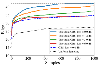
We study the performance of random search algorithms for identifying the planted subgraph, where the strategy is to randomly sample subgraphs and select the densest among all outputs. We compare three different strategies: (i) uniform sampling, (ii) GBS postselected on collision-free outcomes, i.e., outcomes where not more than one photon is detected in each mode, and (iii) GBS with threshold detectors. For threshold GBS, we also investigate the effect of losses, sampling with loss values of $1.2$dB ($25\%$), $3.0$dB ($50\%$), and $6.0$dB ($75\%$). Note that the ability to simulate losses is a unique feature of the algorithm of Ref. quesada2018gaussian .

The results are summarized in Fig. 4. As expected, both loss-free versions of GBS with photon-number-resolving (PNR) and threshold detectors outperform uniform sampling. Interestingly, GBS with threshold detectors performs noticeably better than PNR-based GBS with collision-free postselection. Indeed, threshold GBS consistently finds the planted graph after a few hundred samples. The effect of a threshold detector is equivalent to a post-processing of the PNR outputs where events with two or more photons detected in a mode are considered as a single click in those modes. Thus, our results indicate that retaining collision outputs is beneficial for the purpose of dense subgraph identification, a task that is done automatically by threshold detectors. Moreover, a performance advantage persists for threshold GBS even in the lossy regime. Here, even with a loss of $6.0$dB, threshold GBS is comparable to PNR-based GBS with postselection and no losses.

In this example, we are interested in finding the densest subgraph of 10 vertices. The proportion of $10$ click samples depends on the amount of loss, and we postselect on $4\times 10^{6}$ samples yielding: $4.1\%$ of samples for no losses, $3.2\%$ for $1.2$ dB loss, $2.0\%$ for $3.0$ dB loss, and $0.5\%$ for $6.0$ dB loss. Simulation of each of these cases needed approximately 1000 CPU hours and was completed in less than half an hour using 150 Titan compute nodes each having 16 CPU cores.

Figure 5: Enhancing random search using threshold GBS for dense subgraph identification in the brock200_2 graph johnson1996cliques of Sec. IV.2. Here, the number of edges in the densest found $12$ vertex subgraph is plotted against the number of samples, and lines correspond to sampling from different distributions. Results are averaged over $10$ independent runs. We see that samples from threshold GBS (solid blue line) allow random search to outperform uniform sampling (dashed gray line). The densest subgraph of size $12$ is known to be complete, with $66$ edges, motivating the use of more advanced heuristics and the combination with threshold GBS. It took $30$ gigabytes of memory for each samples, and in total 45,000 core hours to generate 260,000 samples of which we postselect approximately 10,000 samples with 12 clicks.

IV.2 DIMACS graph

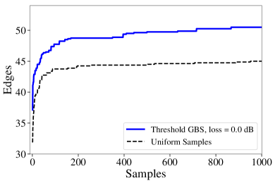
We now investigate the performance of GBS with threshold detectors for dense subgraph identification for a much larger graph of $200$ vertices. We use the brock200_2 graph johnson1996cliques of the DIMACS dataset and search for the densest subgraph with $12$ vertices. The maximum clique, i.e., the largest complete subgraph, of this graph is known to be dimension $12$, meaning that the densest subgraph has $66$ edges. For a graph of this size, it is intractable to perform a brute force GBS postselected on collision-free outcomes.

We use approximately $30$ gigabytes of memory for each sample and a total of $45,000$ core hours to generate $260,000$ samples. Out of these, $9000$ samples with $12$ clicks were postselected , which we use to compare the performance of random search using GBS with threshold detectors to uniform random search. The results are shown in Fig. 5. Here it can also be seen that, as expected, threshold GBS enhances random search. This simple sampling strategy, however, is unable to find the optimum subgraph of $66$ vertices, showcasing the increased difficulty of dense subgraph identification for large graphs. In such cases, it is preferable to combine GBS with more advanced heuristics arrazola2018using .

V Conclusion

Our results constitute the largest simulation of GBS with threshold detectors to date. We have thus set a first goalpost for experiments aiming to build quantum devices capable of outperforming classical algorithms: they must be able to generate enough squeezing to observe more than 20 clicks on average over systems of several hundred modes. The difficulty of classically simulating GBS depends both on the expected number of clicks and the number of modes. The number of clicks in our simulations could thus have in principle been increased at the expense of a smaller number of modes. Regardless, fixing the number of modes as $\ell=2m^{2}$, simulating a sample with $m>22$ clicks is beyond the current capabilities of the Titan supercomputer.

The simulation algorithm of Ref. quesada2018gaussian is ideally suited for benchmarking near-term devices. First, it is an exact sampling algorithm: it generates samples from the GBS distribution, not an approximate one. Second, the algorithm can natively incorporate the effect of experimental imperfections, making it ideal to verify that the physical devices are working adequately and to test the performance of GBS for practical applications, namely identifying dense subgraph.

Currently, the bottleneck of the classical algorithm presented here is the memory usage, which restricts the maximum number of clicks that can be simulated for a given number of modes. Finding more efficient methods of memory allocation or altogether new algorithms is necessary to push simulation capabilities even further. Indeed, it is an important open question whether existing algorithms for boson sampling with indistinguishable single photons can be extended to GBS, where squeezed vacuum inputs are used. These techniques include an approximate algorithm neville2017classical and an exact sampling algorithm clifford2018classical . The complexity of these algorithms is determined by hardness of computing the permanent of a matrix of size given by the number of photons and using supercomputers one can simulate a boson sampling event for approximately 50 photons neville2017classical ; wu2016computing . For GBS, the complexity is determined by the hafnian of matrices with sizes equal to the number of clicks in the sample. Based on the results reported in Ref. bjorklund2018faster , computing the hafnian of a $54\times 54$ matrix requires approximately 1000 seconds on a supercomputer. Therefore, if the techniques of Refs. neville2017classical ; clifford2018classical could be extended to GBS, limits of simulations presented here can be potentially pushed further. So far such an extension is still an open problem.

A python version of the code designed to run on local desktop computers is available at torcode . Optimized code to run large simulations on a supercomputer can be made available upon written request to the authors.

References

- (1) J. Preskill, “Quantum Computing in the NISQ era and beyond”, Quantum 2 (2018) 79.
- (2) A. W. Harrow and A. Montanaro, “Quantum computational supremacy”, Nature 549 (2017), no. 7671, 203.
- (3) E. Pednault, J. A. Gunnels, G. Nannicini, L. Horesh, T. Magerlein, E. Solomonik, and R. Wisnieff, “Breaking the 49-qubit barrier in the simulation of quantum circuits”, arXiv:1710.05867, 2017.
- (4) Z.-Y. Chen, Q. Zhou, C. Xue, X. Yang, G.-C. Guo, and G.-P. Guo, “64-qubit quantum circuit simulation”, Science Bulletin, 2018.
- (5) A. Zulehner and R. Wille, “Advanced simulation of quantum computations”, IEEE Transactions on Computer-Aided Design of Integrated Circuits and Systems, 2018.
- (6) J. D. Biamonte, M. E. Morales, and D. E. Koh, “Quantum supremacy lower bounds by entanglement scaling”, arXiv:1808.00460, 2018.
- (7) J. Chen, F. Zhang, M. Chen, C. Huang, M. Newman, and Y. Shi, “Classical simulation of intermediate-size quantum circuits”, arXiv:1805.01450, 2018.
- (8) S. Aaronson and A. Arkhipov, “The computational complexity of linear optics”, in “Proceedings of the forty-third annual ACM symposium on Theory of computing”, pp. 333–342, ACM. 2011.
- (9) J. B. Spring, B. J. Metcalf, P. C. Humphreys, W. S. Kolthammer, X.-M. Jin, M. Barbieri, A. Datta, N. Thomas-Peter, N. K. Langford, D. Kundys, et al., “Boson sampling on a photonic chip”, Science, 2012 1231692.
- (10) M. A. Broome, A. Fedrizzi, S. Rahimi-Keshari, J. Dove, S. Aaronson, T. C. Ralph, and A. G. White, “Photonic boson sampling in a tunable circuit”, Science 339 (2013), no. 6121, 794–798.
- (11) M. Tillmann, B. Dakić, R. Heilmann, S. Nolte, A. Szameit, and P. Walther, “Experimental boson sampling”, Nature Photonics 7 (2013), no. 7, 540.
- (12) S. Aaronson and A. Arkhipov, “Bosonsampling is far from uniform”, arXiv:1309.7460, 2013.
- (13) A. Lund, A. Laing, S. Rahimi-Keshari, T. Rudolph, J. L. O’Brien, and T. Ralph, “Boson sampling from a gaussian state”, Physical Review Letters 113 (2014), no. 10, 100502.
- (14) M. Bentivegna, N. Spagnolo, C. Vitelli, F. Flamini, N. Viggianiello, L. Latmiral, P. Mataloni, D. J. Brod, E. F. Galvão, A. Crespi, et al., “Experimental scattershot boson sampling”, Science Advances 1 (2015), no. 3, e1400255.
- (15) L. Latmiral, N. Spagnolo, and F. Sciarrino, “Towards quantum supremacy with lossy scattershot boson sampling”, New Journal of Physics 18 (2016), no. 11, 113008.
- (16) C. S. Hamilton, R. Kruse, L. Sansoni, S. Barkhofen, C. Silberhorn, and I. Jex, “Gaussian boson sampling”, Physical Review Letters 119 (2017), no. 17, 170501.
- (17) R. Kruse, C. S. Hamilton, L. Sansoni, S. Barkhofen, C. Silberhorn, and I. Jex, “A detailed study of gaussian boson sampling”, arXiv:1801.07488, 2018.
- (18) J. Huh, G. G. Guerreschi, B. Peropadre, J. R. McClean, and A. Aspuru-Guzik, “Boson sampling for molecular vibronic spectra”, Nature Photonics 9 (2015), no. 9, 615.
- (19) W. R. Clements, J. J. Renema, A. Eckstein, A. A. Valido, A. Lita, T. Gerrits, S. W. Nam, W. S. Kolthammer, J. Huh, and I. A. Walmsley, “Experimental quantum optical approximation of vibronic spectroscopy”, arXiv:1710.08655, 2017.
- (20) C. Sparrow, E. Martín-López, N. Maraviglia, A. Neville, C. Harrold, J. Carolan, Y. N. Joglekar, T. Hashimoto, N. Matsuda, J. L. O’Brien, et al., “Simulating the vibrational quantum dynamics of molecules using photonics”, Nature 557 (2018), no. 7707, 660.
- (21) J. M. Arrazola and T. R. Bromley, “Using gaussian boson sampling to find dense subgraphs”, Phys. Rev. Lett. 121 Jul (2018) 030503.
- (22) J. M. Arrazola, T. R. Bromley, and P. Rebentrost, “Quantum approximate optimization with gaussian boson sampling”, Phys. Rev. A 98 Jul (2018) 012322.
- (23) K. Brádler, P.-L. Dallaire-Demers, P. Rebentrost, D. Su, and C. Weedbrook, “Gaussian boson sampling for perfect matchings of arbitrary graphs”, arXiv:1712.06729, 2017.
- (24) A. Neville, C. Sparrow, R. Clifford, E. Johnston, P. M. Birchall, A. Montanaro, and A. Laing, “Classical boson sampling algorithms with superior performance to near-term experiments”, Nature Physics 13 (2017), no. 12, 1153.
- (25) P. Clifford and R. Clifford, “The classical complexity of boson sampling”, in “Proceedings of the Twenty-Ninth Annual ACM-SIAM Symposium on Discrete Algorithms”, pp. 146–155, SIAM. 2018.
- (26) N. Quesada, J. M. Arrazola, and N. Killoran, “Gaussian boson sampling using threshold detectors”, arXiv:1807.01639, 2018.
- (27) D. S. Johnson and M. A. Trick, “Cliques, coloring, and satisfiability: second dimacs implementation challenge, october 11-13, 1993”, American Mathematical Society, 1996.
- (28) Oak Ridge National Laboratory. https://www.olcf.ornl.gov/olcf-resources/compute-systems/titan/.
- (29) U. Feige, D. Peleg, and G. Kortsarz, “The dense k-subgraph problem”, Algorithmica 29 (2001), no. 3, 410–421.
- (30) R. Kumar, P. Raghavan, S. Rajagopalan, and A. Tomkins, “Trawling the web for emerging cyber-communities”, Computer Networks 31 (1999), no. 11-16, 1481–1493.
- (31) A. Angel, N. Sarkas, N. Koudas, and D. Srivastava, “Dense subgraph maintenance under streaming edge weight updates for real-time story identification”, Proceedings of the VLDB Endowment 5 (2012), no. 6, 574–585.
- (32) A. Beutel, W. Xu, V. Guruswami, C. Palow, and C. Faloutsos, “Copycatch: stopping group attacks by spotting lockstep behavior in social networks”, in “Proceedings of the 22nd international conference on World Wide Web”, pp. 119–130, ACM. New York, 2013.
- (33) J. Chen and Y. Saad, “Dense subgraph extraction with application to community detection”, IEEE Transactions on Knowledge and Data Engineering 24 (2012), no. 7, 1216–1230.
- (34) E. Fratkin, B. T. Naughton, D. L. Brutlag, and S. Batzoglou, “Motifcut: regulatory motifs finding with maximum density subgraphs”, Bioinformatics 22 (2006), no. 14, e150–e157.
- (35) B. Saha, A. Hoch, S. Khuller, L. Raschid, and X.-N. Zhang, “Dense subgraphs with restrictions and applications to gene annotation graphs”, in “Annual International Conference on Research in Computational Molecular Biology”, pp. 456–472, Springer. Berlin, 2010.
- (36) S. Arora, B. Barak, M. Brunnermeier, and R. Ge, “Computational complexity and information asymmetry in financial products”, Communications of the ACM 54 (2011), no. 5, 101–107.
- (37) J. Wu, Y. Liu, B. Zhang, X. Jin, Y. Wang, H. Wang, and X. Yang, “Computing permanents for boson sampling on tianhe-2 supercomputer”, arXiv preprint arXiv:1606.05836, 2016.
- (38) A. Björklund, B. Gupt, and N. Quesada, “A faster hafnian formula for complex matrices and its benchmarking on the titan supercomputer”, arXiv:1805.12498, 2018.
- (39) B. Gupt, “Torontonian sampling code”. https://github.com/XanaduAI/torontonian-sampling, 2018.