\newcites

appReferences

Model-Protected Multi-Task Learning

Jian Liang, Ziqi Liu, Jiayu Zhou, Xiaoqian Jiang, Changshui Zhang, , Fei Wang J. Liang and C. Zhang are with the Department of Automation, Tsinghua University, State Key Laboratory of Intelligent Technologies and Systems, Tsinghua National Laboratory for Information Science and Technology, Beijing, 100084, China.
E-mail: {liangjian12,zcs}@{mails,mail}.tsinghua.edu.cn. Z. Liu was with the Department of Computer Science, Xi’an Jiaotong University, Xi’an, 710049, China. J. Zhou is with the Department of Computer Science and Engineering, Michigan State University, East Lansing, MI, 48824, USA. X. Jiang is with the Department of Biomedical Informatics, University of California, San Diego, La Jolla, CA, 92093, USA. F. Wang is with the Department of Healthcare Policy and Research, Weill Cornell Medical College, New York City, NY, 10065, USA.Manuscript received April 19, 2005; revised August 26, 2015.
Abstract

Multi-task learning (MTL) refers to the paradigm of learning multiple related tasks together. In contrast, in single-task learning (STL) each individual task is learned independently. MTL often leads to better trained models because they can leverage the commonalities among related tasks. However, because MTL algorithms can “leak” information from different models across different tasks, MTL poses a potential security risk. Specifically, an adversary may participate in the MTL process through one task and thereby acquire the model information for another task. The previously proposed privacy-preserving MTL methods protect data instances rather than models, and some of them may underperform in comparison with STL methods. In this paper, we propose a privacy-preserving MTL framework to prevent information from each model leaking to other models based on a perturbation of the covariance matrix of the model matrix. We study two popular MTL approaches for instantiation, namely, learning the low-rank and group-sparse patterns of the model matrix. Our algorithms can be guaranteed not to underperform compared with STL methods. We build our methods based upon tools for differential privacy, and privacy guarantees, utility bounds are provided, and heterogeneous privacy budgets are considered. The experiments demonstrate that our algorithms outperform the baseline methods constructed by existing privacy-preserving MTL methods on the proposed model-protection problem.

Index Terms:
Multi-Task Learning, Model Protection, Differential Privacy, Covariance Matrix, Low-rank Subspace Learning.

1 Introduction

Multi-task learning (MTL) [13] refers to the paradigm of learning multiple related tasks together. In contrast, single-task learning (STL) refers to the paradigm of learning each individual task independently. MTL often leads to better trained models because the commonalities among related tasks may assist in the learning process for each specific task. For example, an infant’s ability to recognize a cat might help in developing the ability to recognize a dog. In recent years, MTL has received considerable interest in a broad range of application areas, including computer vision [48, 75], natural language processing [2] and health informatics [64, 68]. The key to MTL is to relate learning tasks via a shared representation, which, in turn, benefits the tasks to be learned. Each possible shared representation encodes certain assumptions regarding task relatedness. Because MTL approaches explore and leverage the commonalities among related tasks within the learning process, either explicitly or implicitly, they pose a potential security risk. Specifically, an adversary may participate in the MTL process through a participating task, thereby acquiring the model information for another task. A predictive model may identify a causality between system inputs and outputs. Knowledge of the causality makes it possible or easier for an adversary to change a system input to trigger an irrational or even harmful output, which can be regarded as a generalized adversarial attack. The system could be a predictive system for traffic-sign recognition or face identification, as studied by recent adversarial-attack approaches [65, 51, 46, 72, 57, 56, 52]. Pointed out by Finlayson et al. [27], adversarial attacks on medical machine learning are increasingly rampant and easy to implement (e.g., by simply rotating a picture to upload to a specific angle), especially on medical fraud which is a $250 billion industry. Therefore, model-information leakage during an MTL process could realize or escalate such adversarial attacks to increase irrational medical costs or insurances. In addition, the aforementioned system could well be a real human body. For example, consider personalized predictive modeling [53, 74], which has become a fundamental methodology in health informatics. This type of modeling builds a custom-made model for each patient. In modern health informatics, such a model may include patient disease conditions/causes (e.g., which foods can induce an allergic reaction in a patient). If such information were to be leaked, an adversary might use the information to deliberately introduce the food into a patient meal to trigger an allergic reaction, which could be disastrous.

Because of the concerns discussed above, a secure training strategy must be developed for MTL approaches to prevent information from each model leaking to other models. In this paper, we propose a model-protected multi-task learning (MP-MTL) approach that enables the joint learning of multiple related tasks while simultaneously preventing model leakage for each task. We use tools of differential privacy [23] which provides a strong, cryptographically motivated definition of privacy based on rigorous mathematical theory and has recently received significant research attention due to their robustness to known attacks [17, 28]. This scheme is useful when one wishes to prevent potential attackers from acquiring information on any element of the input dataset based on a change in the output distribution.
Refer to caption
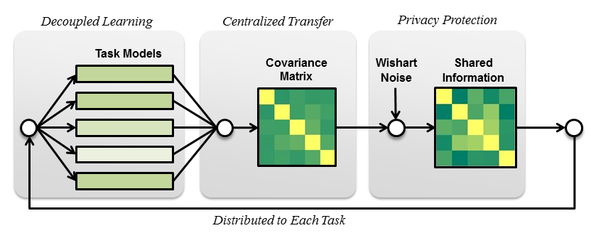
Figure 1: Model-protected multi-task learning framework. The solution process is a recursive two-step procedure. The first step is a decoupled learning procedure in which the model parameters for each task are estimated independently using the precomputed shared information among tasks. The second step is a centralized transfer procedure in which the information shared among tasks is extracted for distribution to each task for the decoupled learning procedure in the next step. The shared information is extracted from the tasks’ covariance matrix, into which Wishart noise is introduced to ensure model security.

To focus on the main issue, our MP-MTL method is designed simply based on linear multi-task models [39, 49]. We assume that the model parameters are learned by minimizing an objective that combines an average empirical prediction loss and a regularization term. The regularization term captures the commonalities among the different tasks and couples their model parameters. The solution process for this type of MTL method can be viewed as a recursive two-step procedure. The first step is a decoupled learning procedure in which the model parameters of each task are estimated independently using some precomputed shared information among tasks. The second step is a centralized transfer procedure in which some of the information shared among tasks is extracted for distribution to each task for the decoupled learning procedure in the next step. Our MP-MTL mechanism protects the models by adding perturbations during the second step. Note that we assume a curator that collects models for joint learning but never needs to collect task data. We develop a rigorous mathematical definition of the MP-MTL problem and propose an algorithmic framework to obtain the solution. We add perturbations to the covariance matrix of the parameter matrix because the tasks’ covariance matrix is widely used as a fundamental source from which to extract useful knowledge to share among tasks [49, 77, 39, 6, 79, 64], which is the key observation that enables the proposed framework. The usage of the perturbed covariance matrix depends on the specific MTL method applied. Consequently, our technique can cover a wide range of MTL algorithms and is generally applicable for many optimization schemes, such as proximal gradient methods [39, 49], alternating methods [6] and Frank-Wolfe methods [37]. We introduce Wishart noise into the covariance matrix to ensure model security. Fig. 1 illustrates the key ideas of the main framework.

We further develop two concrete approaches as instantiations of our framework, each of which transforms an existing MTL algorithm into a private version. Specifically, we consider two popular types of basic MTL models: 1) a model that learns a low-rank subspace by means of a trace norm penalty [39] and 2) a model that performs shared feature selection by means of a group-1subscript1\ell_{1} (2,1subscript21\ell_{2,1} norm) penalty [49]. We first choose to learn a low-rank subspace of the model matrix because it is typical to learn a shared representation, which is the key to relate tasks in MTL. In addition, it is also typical to learn correlated but different parameters for multiple models that share the same model structure, which is also commonly-encountered in MTL. In fact, it is a typical/mainstream approach in MTL, as stated by Zhang and Yang [76] in their MTL survey as well as by Su et al. [63] and Gu et al. [32]; (see, e.g., Ando and Zhang [4]Chen et al. [18]Xu and Lafferty [71]Han and Zhang [35], and Zhen et al. [78]). On the other hand, learning a shared feature selection is also typical in MTL and can be regarded as learning a specific type of low-rank subspace. In both cases, we instantiate our framework by approximating proximal gradient descent methods, which were presented by Ji and Ye [39] and Liu et al. [49]. The covariance matrix is used to build a linear transform matrix used to project the models into new feature subspaces; then, the most useful subspaces are selected. The projection matrix is related to the generalized inverse of the singular value matrix (or the diagonal matrix) of the perturbed covariance matrix for the instantiation with a trace norm penalty (or the instantiation with a group-1subscript1\ell_{1} penalty). Wishart noise is positive definite; thus, it renders the singular values of the perturbed covariance matrix “larger” and those of the generalized inverse “smaller”. Consequently, under a high noise level, the projection matrix tends to be an identity matrix that shares no information between models but keeps the models intact. This means that our algorithms will not underperform in comparison with STL methods under high noise levels; hence, participation in the joint learning process has no negative effect on training any task model. Approximating the proximal operators with Wishart noise makes it possible for the added noise to destroy the covariance matrix without destroying the projected models, which is a key observation that enables the proposed instantiated algorithms.

We provide privacy guarantees. Utility analyses are also presented for both convex and strongly convex prediction loss functions and for both the basic and accelerated proximal-gradient methods. Furthermore, we consider heterogeneous privacy budgets for different iterations of our algorithms and present a utility analysis for privacy-budget allocation. We also validate the effectiveness of our approach on both benchmark and real-world datasets.

Our proposed MP-MTL algorithms fall into a larger scope of differentially private MTL algorithms (i.e., MTL algorithms with randomness added using differential privacy tools). Within this scope, to the best of our knowledge, we are the first to present a utility analysis for heterogeneous tasks. In contrast, the distributed tasks studied by Pathak et al. [58] are homogeneous (i.e., the coding procedures for both features and targets are the same for different tasks). To our knowledge, we are also the first to provide privacy guarantees for heterogeneous tasks and for loss functions without closed-form solutions (e.g., logistic loss).

Since our method are the first to address the model-protected problem in MTL setting, we construct baseline MP-MTL methods for comparison by exploiting existing privacy-preserving MTL methods, which are referred to as instance-protected multi-task learning (IP-MTL) methods because they protect the security only of data instances rather than that of models. The IP-MTL methods are transformed into their respective MP-MTL methods by directly enforcing the group privacy [23] of the entire dataset coming from a single learning task. The experimental results demonstrate that our proposed algorithms outperform the constructed baseline MP-MTL methods.

The contributions of this paper are highlighted as follows.

  • We are the first to propose and address the model-protection problem in an MTL setting.

  • We develop a general algorithmic framework to solve the MP-MTL problem to obtain secure estimates of the model parameters. We derive concrete instantiations of our algorithmic framework for two popular types of MTL models, namely, models that learn the low-rank and group-sparse patterns of the model matrix. By approximating the proximal operators with Wishart noise, we can guarantee that our algorithms will not underperform in comparison with STL methods under high noise levels.

  • We provide privacy guarantees. We also present utility analyses for both convex and strongly convex prediction loss functions and for both the basic and accelerated proximal-gradient methods. Heterogeneous privacy budgets are considered for different iterations of our algorithms, and a utility analysis for privacy-budget allocation is presented.

  • Within the larger scope of differentially private MTL algorithms, to the best of our knowledge, we are the first to provide privacy guarantees for heterogeneous tasks and for loss functions without closed-form solutions. We are also the first to present utility analyses for heterogeneous tasks and the first to present allocation strategies for heterogeneous privacy budgets.

  • For comparison, we construct baseline MP-MTL methods using IP-MTL methods (i.e., existing privacy-preserving MTL methods). The experiments demonstrate that our proposed algorithms significantly outperform the baseline methods.

The remainder of this paper is organized as follows. Section 2 discusses related works and definitions of differential privacy. Section 3 introduces the background on MTL problems and the definition of the proposed model-protection problem. The algorithmic framework and concrete instantiations of the proposed MP-MTL method are presented in Section 4, along with the analyses of utility and privacy-budget allocation. Section 5 presents an empirical evaluation of the proposed approaches, and Section 6 provides conclusions.

2 Related Works

2.1 Privacy-preserving MTL Approaches

Few privacy-preserving MTL approaches have been proposed to date [50, 10, 58, 61, 34]. Moreover, such approaches protect only the security of data instances rather than that of models. A typical focus of research is distributed learning [50, 10], in which the datasets for different tasks are distributively located. The local task models are trained independently using their own datasets before being aggregated and injected with useful knowledge shared across tasks. Such a procedure mitigates the privacy problem by updating each local model independently. However, these methods do not provide theoretical privacy guarantees.

Pathak et al. [58] proposed a differentially private aggregation (DP-AGGR) method in a distributed learning scheme with privacy guarantees in which they first trained local models distributively and then averaged the models of the tasks before adding noise based on the output perturbation method of [21]. The final solution for each task is the averaged model. However, because this method performs only averaging, it has a limited ability to address more complicated task relations such as low-rank [4], group-sparse [66], clustered [31] or graph-based [77] task structures.

Gupta et al. [34] proposed a differentially private multi-task relationship learning (DP-MTRL) method to transform the multi-task relationship learning proposed by Zhang and Yeung [77] into a differentially private version. They adopts the output perturbation method. However, their method requires a closed-form solution (obtained by minimizing the least-square loss function) to achieve a theoretical privacy guarantee; thus, it cannot guarantee privacy for methods such as logistic regression, which requires iterative optimization procedures. Moreover, their privacy-preserving MTL methods underperformed on their synthetic datasets compared with non-private STL methods (which can guarantee optimal privacy against cross-task information leakage), which suggests that there is no reason to use their proposed methods. In addition, they did not study the additional privacy leakage that occurs due to the iterative nature of their algorithm (see Kairouz et al. [42]), and they did not study the utility bound for their method.

The approaches of both Pathak et al. [58] and Gupta et al. [34] protect a single data instance instead of the model of each task, and they involve adding noise directly to the models, which is unnecessary to avoid information leakage across tasks—and may jeopardize the utility of the algorithms.

2.2 Related Works of Differential Privacy

Several related definitions of privacy are listed as follows.

Joint differential privacy. In a game theory setting, Kearns et al. [45] and Kearns et al. [44] proposed to guarantee that for each player, the output to other players reveals little input information about that player. Except for the details of game theory, such as player type, this definition can be regarded as identical to the privacy constraint used in our proposed MP-MTL algorithms.

One-analyst-to-many-analyst privacy. In a database query setting, Hsu et al. [36] proposed a method for protecting the privacy of all the queries of one analyst from other analysts. They also proposed a related privacy called one-query-to-many-analyst privacy. Both privacy definitions can be regarded as identical to the privacy constraints used in our proposed MP-MTL and our defined IP-MTL algorithms, respectively, except for the details of database query.

Roughly speaking, the above approaches and this paper adopt the same privacy constraints but work in different specific fields. This paper leverages these concepts to propose a method to handle the model-protection problem in an MTL setting.

Differential privacy for streams. This definition considers continual/iterative observations, and was proposed by Chan et al. [14] and Dwork et al. [22]. Because machine learning algorithms are generally iterative, this paper also involves the concept of iteration in the definitions of MP-MTL and IP-MTL algorithms, and it simply aims to directly use composition theorems of differential privacy to bound the total privacy-budgets.

Local private learning algorithms. This definition was proposed by Kasiviswanathan et al. [43] to characterize that each individual’s data are added independent randomness before further processing. Algorithms that accomplish this task are referred to as input perturbation. The idea can be adopted to propose possible solutions to the MP-MTL problem. For example, independent randomness can be added to each task model. Both DP-MTRL and DP-AGGR can be regarded as examples, although they protect data instances rather than models. However, because local private learning algorithms have some limitations (e.g., they may require exponentially more data than do general private algorithms  [43]), we did not adopt this idea when constructing our MP-MTL method.

Secure multi-party computation (SMC). In Section 1, we assume the use of a trusted curator that collects the task models, and this assumption raises privacy concerns in untrusted curator settings. Such concerns are related to the demand for SMC [58, 29], the purpose of which is to avoid the leakage of data instances to the curator. We present an extended framework that considers SMC in the supplementary material.

In addition to the above related definitions, the sample-aggregate framework proposed by Nissim et al. [55] is also related. This framework first randomly partitions a database into multiple small databases, executes the same algorithms on all the sub-databases, aggregates all the outputs, and finally adds randomness according to the smooth sensitivity of the aggregation function. For model-protection, this framework may be applicable for homogeneous tasks (which is the setting considered by DP-AGGR) to extend their method for empirical risk minimization: instead of data instances, tasks can be randomly partitioned into groups to perform the above procedures. However, applying this framework to heterogeneous tasks is not trivial. The framework may also be applied to improve the utility of DP-AGGR by smooth sensitivity.

2.3 Methods that Privately Release the Covariance Matrix

Several methods have been proposed to privately release the covariance matrix [41, 24, 11]. Considering an additive noise matrix, based on our utility analysis, the overall utility of the MTL algorithm depends on the spectral norm of the noise matrix. A list of the bounds on the spectral norms of additive noise matrices can be found in Jiang et al. [41]. We choose to add Wishart noise [41] to the covariance matrix for four reasons: (1) For a given privacy budget, this type of noise matrix has a better spectral-norm bound than does a Laplace noise matrix [41]. (2) Unlike a Gaussian noise matrix, which enables an (ϵ,δ)italic-ϵ𝛿(\epsilon,\delta)-private method with a positive δ𝛿\delta, this approach enables an (ϵ,0)italic-ϵ0(\epsilon,0)-private method and can be used to build an iterative algorithm that is entirely (ϵ,0)italic-ϵ0(\epsilon,0)-private, which provides a stronger privacy guarantee. (3) Unlike the Gaussian and Laplace noise matrices cases, the Wishart noise matrix is positive definite and can be exploited to guarantee that our method will not underperform compared with STL methods under high noise levels. (4) This approach allows arbitrary changes to any task, unlike the method of Blocki et al. [11].

3 Preliminaries and the Proposed Problem

In this section, we first introduce the MTL background and then introduce the definition of model-protection problems for MTL.

The notations and symbols that will be used throughout the paper are summarized in Table I.

Table I: Notations and Symbols
[k]delimited-[]𝑘[k] the index set {1,2,,k}12𝑘\{1,2,\cdots,k\}
[i]delimited-[]𝑖[-i] the index set with index i𝑖i removed
\|\cdot\|_{*} the trace norm of a matrix (sum of the singular values of the matrix)
2,1\|\cdot\|_{2,1} the 2,1subscript21\ell_{2,1} norm of a matrix (sum of the 2subscript2\ell_{2} norms of the row vectors of the matrix)
tr()tr{\rm tr(\cdot)} the trace of a matrix (sum of the diagonal elements of the matrix)
σj()subscript𝜎𝑗\sigma_{j}(\cdot) the j𝑗j-th largest singular value of a matrix, j[m]𝑗delimited-[]𝑚j\in[m]

Extensive MTL studies have been conducted on linear models using regularized approaches. The basic MTL algorithm that we consider in this paper is as follows:

𝐖^=argmin𝐖i=1mi(𝐗i𝐰i,𝐲i)+λg(𝐖),^𝐖subscript𝐖superscriptsubscript𝑖1𝑚subscript𝑖subscript𝐗𝑖subscript𝐰𝑖subscript𝐲𝑖𝜆𝑔𝐖\widehat{\mathbf{W}}=\arg\min_{\mathbf{W}}\sum\nolimits_{i=1}^{m}\mathcal{L}_{i}(\mathbf{X}_{i}\mathbf{w}_{i},\mathbf{y}_{i})+\lambda g(\mathbf{W}), (1)

where m𝑚m is the number of tasks. The datasets for the tasks are denoted by 𝒟m=(𝐗m,𝐲m)={(𝐗1,𝐲1),,(𝐗m,𝐲m)}superscript𝒟𝑚superscript𝐗𝑚superscript𝐲𝑚subscript𝐗1subscript𝐲1subscript𝐗𝑚subscript𝐲𝑚\mathcal{D}^{m}=(\mathbf{X}^{m},\mathbf{y}^{m})=\{(\mathbf{X}_{1},\mathbf{y}_{1}),\ldots,(\mathbf{X}_{m},\mathbf{y}_{m})\}, where for each i[m]𝑖delimited-[]𝑚i\in[m], 𝒟i=(𝐗i,𝐲i)subscript𝒟𝑖subscript𝐗𝑖subscript𝐲𝑖\mathcal{D}_{i}=(\mathbf{X}_{i},\mathbf{y}_{i}), where 𝐗ini×dsubscript𝐗𝑖superscriptsubscript𝑛𝑖𝑑\mathbf{X}_{i}\in\mathbb{R}^{n_{i}\times d} and 𝐲ini×1subscript𝐲𝑖superscriptsubscript𝑛𝑖1\mathbf{y}_{i}\in\mathbb{R}^{n_{i}\times 1} denote the data matrix and target vector of the i𝑖i-th task with nisubscript𝑛𝑖n_{i} samples and dimensionality d𝑑d, respectively. isubscript𝑖\mathcal{L}_{i} is the prediction loss function for the i𝑖i-th task. In this paper, we focus on linear MTL models in which 𝐰isubscript𝐰𝑖\mathbf{w}_{i} denotes the model/predictor for task i𝑖i and 𝐖=[𝐰1,𝐰2,,𝐰m]d×m𝐖subscript𝐰1subscript𝐰2subscript𝐰𝑚superscript𝑑𝑚\mathbf{W}=[\mathbf{w}_{1},\mathbf{w}_{2},\cdots,\mathbf{w}_{m}]\in\mathbb{R}^{d\times m} is the model parameter matrix. g()𝑔g(\cdot) is a regularization term that represents the structure of the information shared among the tasks, for which λ𝜆\lambda is a pre-fixed hyper-parameter. As a special case, STL can be described by (1) with λ=0𝜆0\lambda=0.

The key to MTL is to relate the tasks via a shared representation, which, in turn, benefits the tasks to be learned. Each possible shared representation encodes certain assumptions regarding task relatedness.

A typical/mainstream assumption is that the tasks share a latent low-rank subspace, as stated by Zhang and Yang [76] in their survey on MTL, and also by Su et al. [63] and Gu et al. [32]; see, e.g., Ando and Zhang [4]Chen et al. [18]Xu and Lafferty [71]Han and Zhang [35], and Zhen et al. [78]. The formulation leads to a low-rank structure of the model matrix. Because optimization problems involving rank functions are intractable, a trace-norm penalty is typically used [3, 39, 59], as in the following problem, which will be referred to as the trace-norm-regularized MTL problem.

min𝐖i=1mi(𝐗i𝐰i,𝐲i)+λ𝐖.subscript𝐖superscriptsubscript𝑖1𝑚subscript𝑖subscript𝐗𝑖subscript𝐰𝑖subscript𝐲𝑖𝜆subscriptnorm𝐖\min_{\mathbf{W}}\ \sum\nolimits_{i=1}^{m}\mathcal{L}_{i}(\mathbf{X}_{i}\mathbf{w}_{i},\mathbf{y}_{i})+\lambda\|\mathbf{W}\|_{*}. (2)

Another typical assumption is that all tasks share a subset of important features. Such task relatedness can be captured by imposing a group-sparse penalty on the predictor matrix to select shared features across tasks [66, 70, 49]. One commonly used group-sparse penalty is the group 1subscript1\ell_{1} penalty [49, 54], as in the following problem, which will be referred to as the group-1subscript1\ell_{1}-regularized MTL problem.

min𝐖i=1mi(𝐗i𝐰i,𝐲i)+λ𝐖2,1.subscript𝐖superscriptsubscript𝑖1𝑚subscript𝑖subscript𝐗𝑖subscript𝐰𝑖subscript𝐲𝑖𝜆subscriptnorm𝐖21\min_{\mathbf{W}}\ \sum\nolimits_{i=1}^{m}\mathcal{L}_{i}(\mathbf{X}_{i}\mathbf{w}_{i},\mathbf{y}_{i})+\lambda\|\mathbf{W}\|_{2,1}. (3)

Next, we present a compact definition of the model-protection problem in the context of MTL and discuss the general approach without differential privacy. As (1) shows, as a result of the joint learning process, 𝐰^jsubscript^𝐰𝑗\widehat{\mathbf{w}}_{j} may contain some information on 𝐰^isubscript^𝐰𝑖\widehat{\mathbf{w}}_{i}, for i,j[m]𝑖𝑗delimited-[]𝑚i,j\in[m] and ij𝑖𝑗i\neq j, making it possible for the owner of task j𝑗j to use such information to attack task i𝑖i. Thus, we define the model-protection problem as follows.

Definition 1 (Model-protection Problem for MTL).

The model-protection problem for MTL has three objectives:

1) to minimize the information on 𝐰^isubscript^𝐰𝑖\widehat{\mathbf{w}}_{i} that can be inferred from 𝐰^[i]subscript^𝐰delimited-[]𝑖\widehat{\mathbf{w}}_{[-i]}, for all i[m]𝑖delimited-[]𝑚i\in[m];

2) to maximize the prediction performance of 𝐰^isubscript^𝐰𝑖\widehat{\mathbf{w}}_{i}, for all i[m]𝑖delimited-[]𝑚i\in[m]; and

3) to share useful predictive information among tasks.

Now, consider such a procedure in which a trusted curator collects independently-trained models, denoted by 𝐰1,,𝐰msubscript𝐰1subscript𝐰𝑚\mathbf{w}_{1},\ldots,\mathbf{w}_{m}, for all tasks without their associated data to be used as input. After the joint learning process, the curator outputs the updated models, denoted by 𝐖^^𝐖\widehat{\mathbf{W}}, and sends each updated model to each task privately. The model collection and joint learning processes are performed alternately.

We note that the trace-norm-regularized MTL problem and the group-1subscript1\ell_{1}-regularized MTL problem are unified in the multi-task feature learning framework, which is based on the covariance matrix of the tasks’ predictors [7, 25, 8]. Many other MTL methods also fall under this framework, such as learning clustered structures among tasks [31, 79] and inferring task relations [77, 26, 12]. As such, we note that the tasks’ covariance matrix constitutes a major source of shared knowledge in MTL methods; hence, it is regarded as the primary target for model protection.

Therefore, we address the model-protection problem by rephrasing the first objective in Definition 1 as follows: to minimize the changes in 𝐰^[i]subscript^𝐰delimited-[]𝑖\widehat{\mathbf{w}}_{[-i]} and the tasks’ covariance matrix (𝐖^𝐖^T^𝐖superscript^𝐖T\widehat{\mathbf{W}}\widehat{\mathbf{W}}^{\rm T} or 𝐖^T𝐖^superscript^𝐖T^𝐖\widehat{\mathbf{W}}^{\rm T}\widehat{\mathbf{W}}) when task i𝑖i participates in the joint learning process for all i[m]𝑖delimited-[]𝑚i\in[m]. Thus, the model for this new task is protected.

Then, we find that the concept of differential privacy (minimizing the change in the output distribution) can be adopted to further rephrase this objective as follows: to minimize the changes in the distribution of 𝐰^[i]subscript^𝐰delimited-[]𝑖\widehat{\mathbf{w}}_{[-i]} and the tasks’ covariance matrix when task i𝑖i participates in the joint learning process for all i[m]𝑖delimited-[]𝑚i\in[m].

In differential privacy, algorithms are randomized by introducing some type of perturbation.

Definition 2 (Randomized Algorithm).

A randomized algorithm 𝒜:𝒟θ𝒞:𝒜𝒟𝜃𝒞\mathcal{A}:\mathcal{D}\rightarrow\theta\in\mathcal{C} is built by introducing some type of perturbation into some mapping 𝒟θ𝒞𝒟𝜃𝒞\mathcal{D}\rightarrow\theta\in\mathcal{C}. Algorithm 𝒜𝒜\mathcal{A} outputs 𝒜(𝒟)=θ𝒜𝒟𝜃\mathcal{A}(\mathcal{D})=\theta with a density p(𝒜(𝒟)=θ)𝑝𝒜𝒟𝜃p(\mathcal{A}(\mathcal{D})=\theta) for each θ𝒞𝜃𝒞\theta\in\mathcal{C}. The probability space is over the perturbation introduced into algorithm 𝒜𝒜\mathcal{A}.

In this paper, 𝒜𝒜\mathcal{A} denotes some randomized machine learning estimator, and 𝜽𝜽\theta denotes the model parameters that we wish to estimate. Perturbations can be introduced into the original learning system via the (1) input data [47, 9], (2) model parameters [15, 40], (3) objective function [16, 73], or (4) optimization process [62, 69].

The formal definition of differential privacy is as follows.

Definition 3 (Dwork et al. [23]).

A randomized algorithm 𝒜𝒜\mathcal{A} provides (ϵ,δ)italic-ϵ𝛿(\epsilon,\delta)-differential privacy if, for any two adjacent datasets 𝒟𝒟\mathcal{D} and 𝒟superscript𝒟\mathcal{D}^{\prime} that differ by a single entry and for any set 𝒮𝒮\mathcal{S},

(𝒜(𝒟)𝒮)exp(ϵ)(𝒜(𝒟)𝒮)+δ,𝒜𝒟𝒮italic-ϵ𝒜superscript𝒟𝒮𝛿\displaystyle\mathbb{P}(\mathcal{A}(\mathcal{D})\in\mathcal{S})\leq\exp(\epsilon)\mathbb{P}(\mathcal{A}(\mathcal{D}^{\prime})\in\mathcal{S})+\delta,

where 𝒜(𝒟)𝒜𝒟\mathcal{A}(\mathcal{D}) and 𝒜(𝒟)𝒜superscript𝒟\mathcal{A}(\mathcal{D}^{\prime}) are the outputs of 𝒜𝒜\mathcal{A} on the inputs 𝒟𝒟\mathcal{D} and 𝒟superscript𝒟\mathcal{D}^{\prime}, respectively.

The privacy loss pair (ϵ,δ)italic-ϵ𝛿(\epsilon,\delta) is referred to as the privacy budget/loss, and it quantifies the privacy risk of algorithm 𝒜𝒜\mathcal{A}. The intuition is that it is difficult for a potential attacker to infer whether a certain data point has been changed in (or added to) the dataset 𝒟𝒟\mathcal{D} based on a change in the output distribution. Consequently, the information of any single data point is protected.

Furthermore, note that differential privacy is defined in terms of application-specific adjacent input databases. In our setting, these are each task’s model and dataset pair, which are treated as a “single entry” by Definition 3.

Several mechanisms exist for introducing a specific type of perturbation. A typical type is calibrated to the sensitivity of the original “unrandomized” machine learning estimator f:𝒟𝜽d:𝑓𝒟𝜽superscript𝑑f:\mathcal{D}\rightarrow\mbox{\boldmath$\theta$}\in\mathbb{R}^{d}. The sensitivity of an estimator is defined as the maximum change in its output due to a replacement of any single data instance.

Definition 4 (Dwork et al. [23]).

The sensitivity of a function f:𝒟d:𝑓𝒟superscript𝑑f:\mathcal{D}\rightarrow\mathbb{R}^{d} is defined as

S(f)=max𝒟,𝒟f(𝒟)f(𝒟)𝑆𝑓subscript𝒟superscript𝒟norm𝑓𝒟𝑓superscript𝒟\displaystyle S(f)=\max_{\mathcal{D},\mathcal{D}^{\prime}}\|f(\mathcal{D})-f(\mathcal{D}^{\prime})\|

for all datasets 𝒟𝒟\mathcal{D} and 𝒟superscript𝒟\mathcal{D}^{\prime} that differ by at most one instance, where \|\cdot\| is specified by a particular mechanism. For example, the Gaussian mechanism [24] requires the 2subscript2\ell_{2} norm, and the Laplace mechanism [23] requires the 1subscript1\ell_{1} norm.

The use of additive noise such as Laplace  [23] or Gaussian noise [24] with a standard deviation proportional to S(f)𝑆𝑓S(f) is a common practice for guaranteeing private learning. In this paper, we adopt the Wishart noise for covariance matrices [41], which is defined as follows.

Definition 5 (Gupta and Nagar [33]).

A d×d𝑑𝑑d\times d random symmetric positive definite matrix 𝐄𝐄\mathbf{E} is said to have a Wishart distribution 𝐄Wd(ν,𝐕)similar-to𝐄subscript𝑊𝑑𝜈𝐕\mathbf{E}\sim W_{d}(\nu,\mathbf{V}) if its probability density function is

p(𝐄)=|𝐄|(νd1)/2exp(tr(𝐕1𝐄)/2)2νd2|𝐕|1/2Γd(ν/2),𝑝𝐄superscript𝐄𝜈𝑑12trsuperscript𝐕1𝐄2superscript2𝜈𝑑2superscript𝐕12subscriptΓ𝑑𝜈2p(\mathbf{E})=\frac{|\mathbf{E}|^{(\nu-d-1)/2}\exp(-\rm tr(\mathbf{V}^{-1}\mathbf{E})/2)}{2^{\frac{\nu d}{2}}|\mathbf{V}|^{1/2}\Gamma_{d}(\nu/2)},

where ν>d1𝜈𝑑1\nu>d-1 and 𝐕𝐕\mathbf{V} is a d×d𝑑𝑑d\times d positive definite matrix.

Because machine learning schemes are usually presented as sequential paradigms with multiple iterations and usually output multiple variables simultaneously, several differential privacy properties are particularly useful for ensuring privacy in machine learning, such as post-processing immunity, group privacy, composition properties and adaptive composition. The details of these properties are introduced in the supplementary material.

4 Methodology

We present our methodology in this section: the modeling of and rationale for our MP-MTL framework, two instantiations and utility analyses. Regarding the theoretical results, we present only the main results; the detailed derivations are included in the provided supplementary material.

4.1 The General MP-MTL Framework

Consider an MTL algorithm 𝒜𝒜\mathcal{A} with T𝑇T iterations. For t=1,,T𝑡1𝑇t=1,\ldots,T, a trusted curator collects the models of m𝑚m tasks, respectively, denoted by 𝐰1(t1),,𝐰m(t1)superscriptsubscript𝐰1𝑡1superscriptsubscript𝐰𝑚𝑡1\mathbf{w}_{1}^{(t-1)},\ldots,\mathbf{w}_{m}^{(t-1)}. Then, a model-protection and shared-information-extraction procedure is performed, and the updated models 𝐰^1(t),,𝐰^m(t)superscriptsubscript^𝐰1𝑡superscriptsubscript^𝐰𝑚𝑡\hat{\mathbf{w}}_{1}^{(t)},\ldots,\hat{\mathbf{w}}_{m}^{(t)} are output and sent back to their respective tasks.

Remark 1.

Note that in each iteration, the curator collects only the models. The dataset for each task can be regarded as the input for the entire MTL algorithm, but it is not the input for the curator.

In such a setting, for each i[m]𝑖delimited-[]𝑚i\in[m], we wish to protect the dataset 𝒟i=(𝐗i,𝐲i)subscript𝒟𝑖subscript𝐗𝑖subscript𝐲𝑖\mathcal{D}_{i}=(\mathbf{X}_{i},\mathbf{y}_{i}) of task i𝑖i and its entire input model-sequence (𝐰i(0),,𝐰i(T1))superscriptsubscript𝐰𝑖0superscriptsubscript𝐰𝑖𝑇1(\mathbf{w}_{i}^{(0)},...,\mathbf{w}_{i}^{(T-1)}) (denoted by 𝐰i(0:T1)superscriptsubscript𝐰𝑖:0𝑇1\mathbf{w}_{i}^{(0:T-1)} for short). For the i𝑖i-th task, the entire output model-sequence of other tasks, 𝐰^[i](1:T)superscriptsubscript^𝐰delimited-[]𝑖:1𝑇\hat{\mathbf{w}}_{[-i]}^{(1:T)}, is the view of a potential adversary (i.e., the information that the adversary can acquire to infer the unique information of task i𝑖i). Note that although the output model-sequence of each task is what we ultimately wish to protect, the unique information within each task is contained in the task’s dataset and input model-sequence, which are actually protected.

The idea for using differental privacy tools is as follows. For simpilicity, we assume that T=1𝑇1T=1 and omit the iteration-step indices. Let 𝒟~={(𝐰1,𝒟1),,(𝐰m,𝒟m)}~𝒟subscript𝐰1subscript𝒟1subscript𝐰𝑚subscript𝒟𝑚\widetilde{\mathcal{D}}=\{(\mathbf{w}_{1},\mathcal{D}_{1}),\ldots,(\mathbf{w}_{m},\mathcal{D}_{m})\} be an augmented dataset; i.e., let (𝐰i,𝒟i)subscript𝐰𝑖subscript𝒟𝑖(\mathbf{w}_{i},\mathcal{D}_{i}) be treated as the i𝑖i-th “data instance” of the augmented dataset 𝒟~~𝒟\widetilde{\mathcal{D}}, for all i[m]𝑖delimited-[]𝑚i\in[m]. Thus, the m𝑚m datasets and m𝑚m models associated with the m𝑚m tasks are transformed into a single dataset 𝒟~~𝒟\widetilde{\mathcal{D}} with m𝑚m “data instances”. Then, we define m𝑚m outputs 𝜽=(θ1,,θm)𝜽subscript𝜃1subscript𝜃𝑚\mbox{\boldmath$\theta$}=(\theta_{1},\ldots,\theta_{m}) such that for each i[m]𝑖delimited-[]𝑚i\in[m], θi𝒞isubscript𝜃𝑖subscript𝒞𝑖\theta_{i}\in\mathcal{C}_{i} denotes the view of an adversary for task i𝑖i, which includes 𝐰^[i]subscript^𝐰delimited-[]𝑖\hat{\mathbf{w}}_{[-i]}. Thus, an (ϵ,δ)italic-ϵ𝛿(\epsilon,\delta) - MP-MTL algorithm 𝒜()𝒜\mathcal{A}(\mathcal{B}) should satisfy the following m𝑚m inequalities. For each i[m]𝑖delimited-[]𝑚i\in[m], for all neighboring datasets 𝒟~~𝒟\widetilde{\mathcal{D}} and 𝒟~superscript~𝒟\widetilde{\mathcal{D}}^{\prime} that differ by the i𝑖i-th “data instance”, and for any set 𝒮iCisubscript𝒮𝑖subscript𝐶𝑖\mathcal{S}_{i}\subseteq C_{i}, we have

(θi𝒮i=𝒟~)eϵ(θi𝒮i=𝒟~)+δ.subscript𝜃𝑖conditionalsubscript𝒮𝑖~𝒟superscript𝑒italic-ϵsubscript𝜃𝑖conditionalsubscript𝒮𝑖superscript~𝒟𝛿\begin{split}\mathbb{P}&(\theta_{i}\in\mathcal{S}_{i}\mid\mathcal{B}=\widetilde{\mathcal{D}})\leq e^{\epsilon}\mathbb{P}(\theta_{i}\in\mathcal{S}_{i}\mid\mathcal{B}=\widetilde{\mathcal{D}}^{\prime})+\delta.\end{split} (4)

We formally define an MP-MTL algorithm as follows.

Definition 6 (MP-MTL).

Let 𝒜𝒜\mathcal{A} be a randomized MTL algorithm with a number of iterations T𝑇T. In the first iteration, 𝒜𝒜\mathcal{A} performs the mapping (𝐖(0)d×m,𝒟m)θ1𝒞1superscript𝐖0superscript𝑑𝑚superscript𝒟𝑚subscript𝜃1subscript𝒞1(\mathbf{W}^{(0)}\in\mathbb{R}^{d\times m},\mathcal{D}^{m})\rightarrow\theta_{1}\in\mathcal{C}_{1}, where θ1subscript𝜃1\theta_{1} includes 𝐖^(1)d×msuperscript^𝐖1superscript𝑑𝑚\widehat{\mathbf{W}}^{(1)}\in\mathbb{R}^{d\times m}. For t=2,,T𝑡2𝑇t=2,\ldots,T, in the t𝑡t-th iteration, 𝒜𝒜\mathcal{A} performs the mapping (𝐖(t1)d×m,𝒟m,θ1,,θt1)θt𝒞tsuperscript𝐖𝑡1superscript𝑑𝑚superscript𝒟𝑚subscript𝜃1subscript𝜃𝑡1subscript𝜃𝑡subscript𝒞𝑡(\mathbf{W}^{(t-1)}\in\mathbb{R}^{d\times m},\mathcal{D}^{m},\theta_{1},\ldots,\theta_{t-1})\rightarrow\theta_{t}\in\mathcal{C}_{t}, where θtsubscript𝜃𝑡\theta_{t} includes 𝐖^(t)d×msuperscript^𝐖𝑡superscript𝑑𝑚\widehat{\mathbf{W}}^{(t)}\in\mathbb{R}^{d\times m}. Then, 𝒜𝒜\mathcal{A} is an (ϵ,δ)italic-ϵ𝛿(\epsilon,\delta) - MP-MTL algorithm if for all i[m]𝑖delimited-[]𝑚i\in[m], for all t[T]𝑡delimited-[]𝑇t\in[T], and for neighboring input pairs (𝐖(t1),𝒟m)superscript𝐖𝑡1superscript𝒟𝑚(\mathbf{W}^{(t-1)},\mathcal{D}^{m}) and ((𝐖)(t1),(𝒟)m)superscriptsuperscript𝐖𝑡1superscriptsuperscript𝒟𝑚((\mathbf{W}^{\prime})^{(t-1)},(\mathcal{D}^{\prime})^{m}) that differ only by the i𝑖i-th task such that 𝐰i(t1)(𝐰i)(t1)superscriptsubscript𝐰𝑖𝑡1superscriptsubscriptsuperscript𝐰𝑖𝑡1\mathbf{w}_{i}^{(t-1)}\neq(\mathbf{w}^{\prime}_{i})^{(t-1)} or 𝒟i𝒟isubscript𝒟𝑖subscriptsuperscript𝒟𝑖\mathcal{D}_{i}\neq\mathcal{D}^{\prime}_{i}, the following holds for some constants ϵ,δ0italic-ϵ𝛿0\epsilon,\delta\geq 0 and for any set 𝒮d×(m1)×T𝒮superscript𝑑𝑚1𝑇\mathcal{S}\subseteq\mathbb{R}^{d\times(m-1)\times T}:

(𝐰^[i](1:T)𝒮t=1Tt=(𝐖(t1),𝒟m,𝜽1:t1))eϵ(𝐰^[i](1:T)𝒮t=1Tt=((𝐖)(t1),(𝒟)m,𝜽1:t1))+δ,superscriptsubscript^𝐰delimited-[]𝑖:1𝑇𝒮superscriptsubscript𝑡1𝑇subscript𝑡superscript𝐖𝑡1superscript𝒟𝑚subscript𝜽:1𝑡1superscript𝑒italic-ϵsuperscriptsubscript^𝐰delimited-[]𝑖:1𝑇conditional𝒮superscriptsubscript𝑡1𝑇subscript𝑡superscriptsuperscript𝐖𝑡1superscriptsuperscript𝒟𝑚subscript𝜽:1𝑡1𝛿\begin{split}\mathbb{P}(&\hat{\mathbf{w}}_{[-i]}^{(1:T)}\in\mathcal{S}\mid\bigcap_{t=1}^{T}\mathcal{B}_{t}=(\mathbf{W}^{(t-1)},\mathcal{D}^{m},\mbox{\boldmath$\theta$}_{1:t-1}))\\ \leq&e^{\epsilon}\mathbb{P}(\hat{\mathbf{w}}_{[-i]}^{(1:T)}\in\mathcal{S}\mid\bigcap_{t=1}^{T}\mathcal{B}_{t}=((\mathbf{W}^{\prime})^{(t-1)},(\mathcal{D}^{\prime})^{m},\mbox{\boldmath$\theta$}_{1:t-1}))\\ &+\delta,\end{split} (5)

where for all t[T]𝑡delimited-[]𝑇t\in[T], tsubscript𝑡\mathcal{B}_{t} denotes the input for the t𝑡t-th iteration and

𝜽1:t1=subscript𝜽:1𝑡1absent\displaystyle\mbox{\boldmath$\theta$}_{1:t-1}= ,\displaystyle\emptyset, t=1𝑡1t=1
𝜽1:t1=subscript𝜽:1𝑡1absent\displaystyle\mbox{\boldmath$\theta$}_{1:t-1}= θ1,θ2,,θt1,subscript𝜃1subscript𝜃2subscript𝜃𝑡1\displaystyle\theta_{1},\theta_{2},\cdots,\theta_{t-1}, t2𝑡2t\geq 2.

Note that in Definition 6, we view the model sequence 𝐰^[i](1:T)superscriptsubscript^𝐰delimited-[]𝑖:1𝑇\hat{\mathbf{w}}_{[-i]}^{(1:T)} as a single output of the algorithm for each task i[m]𝑖delimited-[]𝑚i\in[m]. The definition of neighboring inputs allows the model and dataset for any task to change in all rounds of the iterative optimization rather than in only a single round. Definition 6 defines a privacy constraint for MTL algorithms. Roughly speaking, this privacy constraint can be regarded as identical to joint differential privacy [45, 44] or to one-analyst-to-many-analyst privacy [36], despite detailed differences between MTL, game theory, and database queries.

STL can easily be shown to be optimal for avoiding information leakage across tasks because the individual task models are learned independently.

Claim 1.

Any STL algorithm that learns each task independently is a (0,0)00(0,0) - MP-MTL algorithm.

From this claim, we learn that when no information sharing occurs across tasks, no leakage can occur across tasks.

Our MP-MTL framework is elaborated in Algorithm 1, which considers heterogeneous privacy budgets for different iteration steps. To maintain the total privacy budget below than a specified value using the adaptive composition theorem provided by Kairouz et al. [42], we define a composition bound of a series of privacy budgets as follows (the equation is taken directly from Theorem 3.5 of Kairouz et al. [42]):

Definition 7 (Composition Bound of Privacy Budgets).

For an integer T1𝑇1T\geq 1, a series of privacy budgets, ϵ1,,ϵT0subscriptitalic-ϵ1subscriptitalic-ϵ𝑇0\epsilon_{1},\ldots,\epsilon_{T}\geq 0, a specified privacy loss δ0𝛿0\delta\geq 0, the composition bound of {ϵt}subscriptitalic-ϵ𝑡\{\epsilon_{t}\} is defined as CB({ϵt},δ)𝐶𝐵subscriptitalic-ϵ𝑡𝛿CB(\{\epsilon_{t}\},\delta), which equals

min{t=1Tϵt,t=1T(eϵt1)ϵt(eϵt+1)+t=1T2ϵt2log(1δ),t=1T(eϵt1)ϵt(eϵt+1)+t=1T2ϵt2log(e+t=1Tϵt2δ)}.superscriptsubscript𝑡1𝑇subscriptitalic-ϵ𝑡superscriptsubscript𝑡1𝑇superscript𝑒subscriptitalic-ϵ𝑡1subscriptitalic-ϵ𝑡superscript𝑒subscriptitalic-ϵ𝑡1superscriptsubscript𝑡1𝑇2superscriptsubscriptitalic-ϵ𝑡21𝛿superscriptsubscript𝑡1𝑇superscript𝑒subscriptitalic-ϵ𝑡1subscriptitalic-ϵ𝑡superscript𝑒subscriptitalic-ϵ𝑡1superscriptsubscript𝑡1𝑇2superscriptsubscriptitalic-ϵ𝑡2𝑒superscriptsubscript𝑡1𝑇superscriptsubscriptitalic-ϵ𝑡2𝛿\begin{split}&\min\biggl{\{}\sum_{t=1}^{T}\epsilon_{t},\sum_{t=1}^{T}\frac{(e^{\epsilon_{t}}-1)\epsilon_{t}}{(e^{\epsilon_{t}}+1)}+\sqrt{\sum_{t=1}^{T}2\epsilon_{t}^{2}\log\biggl{(}\frac{1}{\delta}\biggr{)}},\\ &\sum_{t=1}^{T}\frac{(e^{\epsilon_{t}}-1)\epsilon_{t}}{(e^{\epsilon_{t}}+1)}+\sqrt{\sum_{t=1}^{T}2\epsilon_{t}^{2}\log\biggl{(}e+\frac{\sqrt{\sum_{t=1}^{T}\epsilon_{t}^{2}}}{\delta}\biggr{)}}\biggr{\}}.\end{split} (6)

In Algorithm 1, as mentioned in Section 3, we choose to protect the tasks’ covariance matrix, which is denoted by 𝚺=𝐖𝐖T𝚺superscript𝐖𝐖T\mbox{\boldmath$\Sigma$}=\mathbf{W}\mathbf{W}^{\rm T} or 𝚺=𝐖T𝐖𝚺superscript𝐖T𝐖\mbox{\boldmath$\Sigma$}=\mathbf{W}^{\rm T}\mathbf{W}, depending on the MTL method selected. As previously stated, Wishart noise [41] is added. Fig. 1 illustrates the key concepts of the framework. In detail, Step 1 of Algorithm 1 ensures that the total privacy budgets satisfy the specified values ϵitalic-ϵ\epsilon and δ𝛿\delta, respectively. The purpose of norm clipping in Step 3 is simply to render the models in a bounded space, which help us compute a proper noise scale to add to satisfy the privacy constraint defined in Definition 6. Step 4 extracts the shared information between tasks—the tasks’ covariance matrix. Step 5 adds a perturbation into the shared information. Step 6 further extracts useful information from the perturbed covariance matrix. Step 7 sends the extracted useful information to each task to perform decoupled learning. If no noise is added, Steps 4–7 could be a proximal gradient descent step, i.e., first performing a proximal operator step and then taking a gradient descent step; see, e.g., Ji and Ye [39] and Liu et al. [49]. This framework is generally applicable for many optimization schemes, such as proximal gradient methods [39, 49], alternating methods [6] and Frank-Wolfe methods [37].

Note that we mainly provided theoretical and experimental results for the 𝐖𝐖Tsuperscript𝐖𝐖T\mathbf{W}\mathbf{W}^{\rm T} type of covariance matrix. Nonetheless, the 𝐖T𝐖superscript𝐖T𝐖\mathbf{W}^{\rm T}\mathbf{W} type of covariance matrix can be regarded as a natural alternative, since it was successfully used by Zhang and Yeung [77] (as a non-private method), Gupta et al. [34] (as a differentially private method), and all the subsequent MTL methods to learn relationships between tasks (see, e.g., the task-relation learning approaches introduced by Zhang and Yang [76] in Section 2.4 of their survey on MTL). Therefore, we included it in our framework.

Remark 2.

In Algorithm 1, a curator who collects models and performs centralized transfer needs to run only Steps 4–6 and does not need to collect the datasets (𝐗m,𝐲m)superscript𝐗𝑚superscript𝐲𝑚(\mathbf{X}^{m},\mathbf{y}^{m}), which are used only in STL algorithms.

Algorithm 1 MP-MTL framework
0:  Datasets (𝐗m,𝐲m)={(𝐗1,𝐲1),,(𝐗m,𝐲m)}superscript𝐗𝑚superscript𝐲𝑚subscript𝐗1subscript𝐲1subscript𝐗𝑚subscript𝐲𝑚(\mathbf{X}^{m},\mathbf{y}^{m})=\{(\mathbf{X}_{1},\mathbf{y}_{1}),\ldots,(\mathbf{X}_{m},\mathbf{y}_{m})\}, where i[m],𝐗ini×dformulae-sequencefor-all𝑖delimited-[]𝑚subscript𝐗𝑖superscriptsubscript𝑛𝑖𝑑\forall i\in[m],\ \mathbf{X}_{i}\in\mathbb{R}^{n_{i}\times d} and 𝐲ini×1subscript𝐲𝑖superscriptsubscript𝑛𝑖1\mathbf{y}_{i}\in\mathbb{R}^{n_{i}\times 1}. Privacy loss ϵ,δ0italic-ϵ𝛿0\epsilon,\delta\geq 0. Number of iterations T𝑇T. Initial shared information matrix 𝐌(0)superscript𝐌0\mathbf{M}^{(0)}. Initial task models 𝐖(0)superscript𝐖0\mathbf{W}^{(0)}, which can be acquired via arbitrary STL methods.
0:  𝐖^(1:T)superscript^𝐖:1𝑇\widehat{\mathbf{W}}^{(1:T)} .
1:  Set {ϵt}subscriptitalic-ϵ𝑡\{\epsilon_{t}\} such that CB({ϵt},δ)ϵ𝐶𝐵subscriptitalic-ϵ𝑡𝛿italic-ϵCB(\{\epsilon_{t}\},\delta)\leq\epsilon, where CB({ϵt},δ)𝐶𝐵subscriptitalic-ϵ𝑡𝛿CB(\{\epsilon_{t}\},\delta) is the composition bound of {ϵt}subscriptitalic-ϵ𝑡\{\epsilon_{t}\}.
2:  for t=1:T:𝑡1𝑇t=1:T do
3:     Norm clipping: 𝐰~i(t1)=𝐰i(t1)/max(1,𝐰i(t1)2K)superscriptsubscript~𝐰𝑖𝑡1superscriptsubscript𝐰𝑖𝑡11subscriptnormsuperscriptsubscript𝐰𝑖𝑡12𝐾\tilde{\mathbf{w}}_{i}^{(t-1)}={\mathbf{w}}_{i}^{(t-1)}/\max(1,\frac{\|{\mathbf{w}}_{i}^{(t-1)}\|_{2}}{K}), for all i[m]𝑖delimited-[]𝑚i\in[m]. Let 𝐖^(0)=𝐖~(0)superscript^𝐖0superscript~𝐖0\widehat{\mathbf{W}}^{(0)}=\widetilde{\mathbf{W}}^{(0)}.
4:     𝚺~(t)=𝐖~(t1)(𝐖~(t1))Tsuperscript~𝚺𝑡superscript~𝐖𝑡1superscriptsuperscript~𝐖𝑡1T\widetilde{\mbox{\boldmath$\Sigma$}}^{(t)}=\widetilde{\mathbf{W}}^{(t-1)}(\widetilde{\mathbf{W}}^{(t-1)})^{\rm T} (or 𝚺~(t)=(𝐖~(t1))T𝐖~(t1)superscript~𝚺𝑡superscriptsuperscript~𝐖𝑡1Tsuperscript~𝐖𝑡1\widetilde{\mbox{\boldmath$\Sigma$}}^{(t)}=(\widetilde{\mathbf{W}}^{(t-1)})^{\rm T}\widetilde{\mathbf{W}}^{(t-1)}).
5:     𝚺(t)=𝚺~(t)+𝐄superscript𝚺𝑡superscript~𝚺𝑡𝐄\mbox{\boldmath$\Sigma$}^{(t)}=\widetilde{\mbox{\boldmath$\Sigma$}}^{(t)}+\mathbf{E}, where 𝐄Wd(d+1,K22ϵt𝐈d)similar-to𝐄subscript𝑊𝑑𝑑1superscript𝐾22subscriptitalic-ϵ𝑡subscript𝐈𝑑\mathbf{E}\sim W_{d}(d+1,\frac{K^{2}}{2\epsilon_{t}}\mathbf{I}_{d}) (or 𝐄Wm(m+1,K22ϵt𝐈m)similar-to𝐄subscript𝑊𝑚𝑚1superscript𝐾22subscriptitalic-ϵ𝑡subscript𝐈𝑚\mathbf{E}\sim W_{m}(m+1,\frac{K^{2}}{2\epsilon_{t}}\mathbf{I}_{m})) is a sample from the Wishart distribution, 𝐈dsubscript𝐈𝑑\mathbf{I}_{d} denotes the d×d𝑑𝑑d\times d identity matrix, and diag()diag\mbox{diag}(\cdot) transforms a vector into a diagonal matrix.
6:     Perform an arbitrary mapping f:𝚺(1:t)𝐌(t):𝑓superscript𝚺:1𝑡superscript𝐌𝑡f:\mbox{\boldmath$\Sigma$}^{(1:t)}\rightarrow\mathbf{M}^{(t)}, e.g., take the diagonal elements of 𝚺(t)superscript𝚺𝑡\mbox{\boldmath$\Sigma$}^{(t)} or the singular value decomposition of 𝚺(t)superscript𝚺𝑡\mbox{\boldmath$\Sigma$}^{(t)}.
7:     𝐰^i(t)=𝒜st,i(𝐌(t),𝐰~i(0:t1),𝐗i,𝐲i)superscriptsubscript^𝐰𝑖𝑡subscript𝒜st𝑖superscript𝐌𝑡superscriptsubscript~𝐰𝑖:0𝑡1subscript𝐗𝑖subscript𝐲𝑖\hat{\mathbf{w}}_{i}^{(t)}=\mathcal{A}_{\mbox{st},i}(\mathbf{M}^{(t)},\tilde{\mathbf{w}}_{i}^{(0:t-1)},\mathbf{X}_{i},\mathbf{y}_{i}), for all i[m]𝑖delimited-[]𝑚i\in[m], where 𝒜st,isubscript𝒜st𝑖\mathcal{A}_{\mbox{st},i} is an arbitrary STL algorithm for the i𝑖i-th task and the 𝐰~i(0:t1)superscriptsubscript~𝐰𝑖:0𝑡1\tilde{\mathbf{w}}_{i}^{(0:t-1)} are used for initialization.
8:     Set the input for the next iteration: 𝐖(t)=𝐖^(t)superscript𝐖𝑡superscript^𝐖𝑡\mathbf{W}^{(t)}=\widehat{\mathbf{W}}^{(t)}.
9:  end for

4.2 Instantiations of the MP-MTL Framework

In this section, we instantiate our MP-MTL framework (described in Algorithm 1) by approximating the proximal gradient descent methods presented by Ji and Ye [39] and Liu et al. [49] for the trace-norm-regularized MTL problem and the group-1subscript1\ell_{1}-regularized MTL problem, respectively. Both proximal gradient descent methods solve the respective MTL problems by alternately performing a proximal operator step and a gradient descent step. Taking the trace-norm-regularized MTL problem as an example, the loss function, iisubscript𝑖subscript𝑖\sum_{i}\mathcal{L}_{i}, is minimized by the gradient descent steps, while the regularization term, the trace-norm, is minimized by the proximal operator steps. The proximal operator minimizes the regularization term, keeping the variable near the result of a previous gradient descent step. Specifically, we instantiate Steps 4–7 of Algorithm 1 by approximating a proximal gradient descent step, i.e., first performing a proximal operator step and then taking a gradient descent step. It is similar for the group-1subscript1\ell_{1}-regularized MTL problem but the difference lies in the instantiations of Step 6 of Algorithm 1 because different regularization terms lead to different optimal solutions for the proximal operators. Note that both instantiations use the 𝐖𝐖Tsuperscript𝐖𝐖T\mathbf{W}\mathbf{W}^{\rm T} type of covariance matrix, which is required by the optimal solutions [39, 49].

First, we instantiate the MP-MTL framework for the trace-norm-regularized MTL problem, as shown in Algorithm 2. Generally speaking, the algorithm uses an accelerated proximal gradient method. Steps 49 approximate the following proximal operator [39]:

𝐖^(t1)=argmin𝐖12η𝐖𝐖~(t1)F2+λ𝐖,superscript^𝐖𝑡1subscript𝐖12𝜂superscriptsubscriptnorm𝐖superscript~𝐖𝑡1𝐹2𝜆subscriptnorm𝐖\displaystyle\widehat{\mathbf{W}}^{(t-1)}=\arg\min_{\mathbf{W}}\frac{1}{2\eta}\|\mathbf{W}-\widetilde{\mathbf{W}}^{(t-1)}\|_{F}^{2}+\lambda\|\mathbf{W}\|_{*}, (7)

where 𝐖~(t1)superscript~𝐖𝑡1\widetilde{\mathbf{W}}^{(t-1)} can be regarded as the result of the gradient descent step in the previous iteration, assuming K𝐾K is sufficiently large. In detail, Steps 6–8 of Algorithm 2 instantiate Step 6 of Algorithm 1 by constructing a projection matrix, 𝐌(t)=𝐔𝐒ηλ𝐔Tsuperscript𝐌𝑡subscript𝐔𝐒𝜂𝜆superscript𝐔T\mathbf{M}^{(t)}=\mathbf{U}\mathbf{S}_{\eta\lambda}\mathbf{U}^{\rm T}, from the result of singular vector decomposition of the perturbed covariance matrix. Steps 9–11 of Algorithm 2 instantiate Step 7 of Algorithm 1 by first projecting the models (in Step 9) and then performing accelerated gradient descent.
Refer to caption
(a) Before MTL
Refer to caption
(b) After MTL with model leakage
Refer to caption
(c) After MTL with model protection
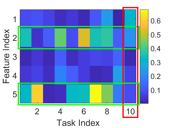
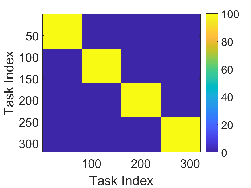
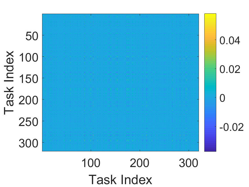
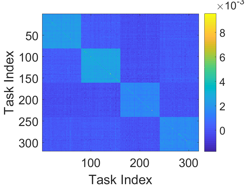
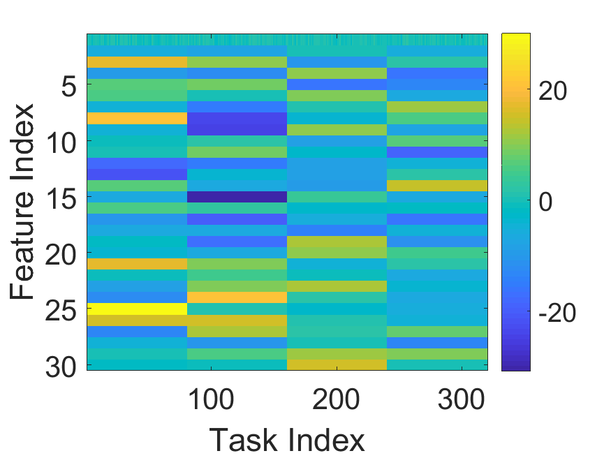
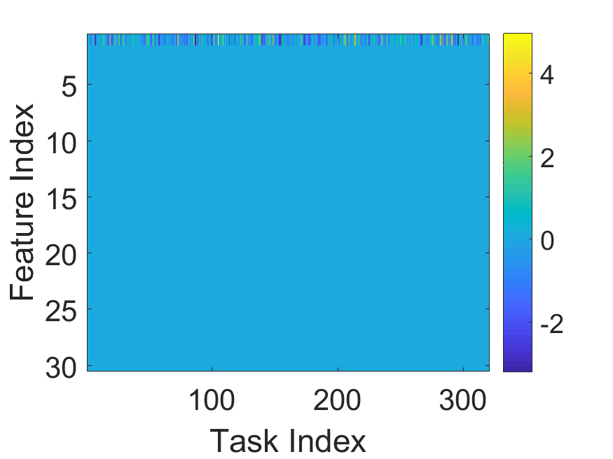
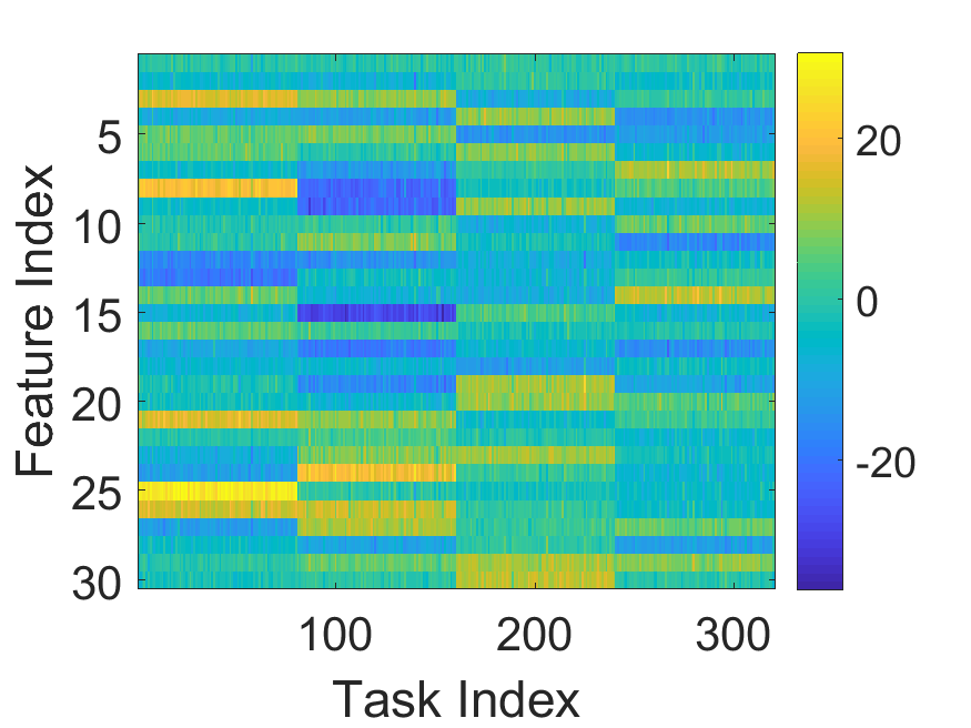
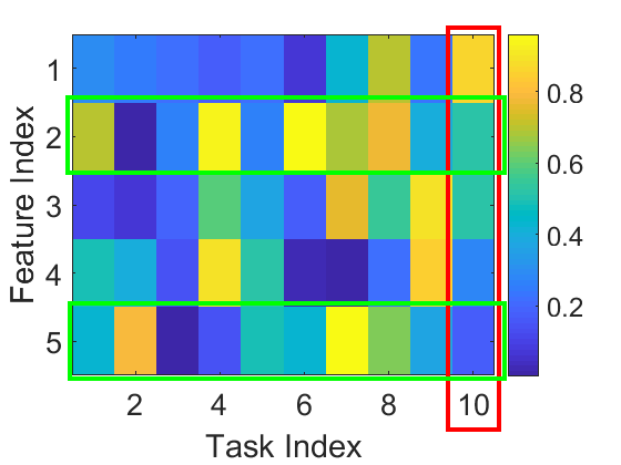
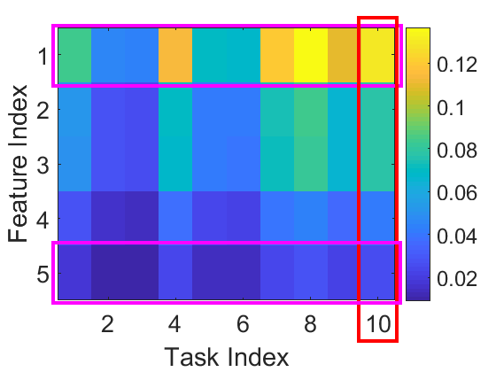
Figure 2: Examples of model leakage and model protection showing model matrices, where columns correspond to tasks and rows correspond to features. The columns shown have been divided by their respective 2subscript2\ell_{2} norms.

We provide a running example for model leakage and model protection under different settings of Algorithm 2, as shown in Fig. 2. We generate models for m=10𝑚10m=10 tasks, in which the data dimension is d=5𝑑5d=5. The 10th task (the rightmost one), is an anomaly task that requires privacy protection. In Fig. 2 (a), the matrix denoted by 𝐖(0)superscript𝐖0\mathbf{W}^{(0)} is first generated from an i.i.d. uniform distribution 𝒰(0,1)𝒰01\mathcal{U}(0,1). Then, the rightmost column is multiplied by 100100100. For MTL with model leakage, we execute Algorithm 2, setting T=1,η=1,ϵ1=ϵ=1e40,δ=0,K=1005formulae-sequenceformulae-sequence𝑇1formulae-sequence𝜂1subscriptitalic-ϵ1italic-ϵ1𝑒40formulae-sequence𝛿0𝐾1005T=1,\eta=1,\epsilon_{1}=\epsilon=1e40,\delta=0,K=100\sqrt{5} and λ=50𝜆50\lambda=50. It can be regarded that the noise matrix 𝐄𝐄\mathbf{E} is not added, since ϵ1much-greater-thanitalic-ϵ1\epsilon\gg 1. The output model matrix 𝐖^(1)superscript^𝐖1\widehat{\mathbf{W}}^{(1)} is shown in Fig. 2 (b), in which the 10th task results in significantly influences on the parameters of other models: other models’ parameters are similar to those of the 10th task, e.g., for each task, the first feature is the biggest, and the fifth feature is the smallest. For MTL with model protection, we execute Algorithm 2 with the same setting as above except that we set ϵ1=ϵ=0.1subscriptitalic-ϵ1italic-ϵ0.1\epsilon_{1}=\epsilon=0.1. The output model matrix 𝐖^(1)superscript^𝐖1\widehat{\mathbf{W}}^{(1)} is shown in Fig. 2 (c), in which the influences from the 10th task are not significant: other models’ parameters are not similar to those of the 10th task. Meanwhile, for 𝐖(0)superscript𝐖0\mathbf{W}^{(0)}, shown in Fig. 2 (a), for tasks 1-9, the 2subscript2\ell_{2} norms of the second and the fifth rows are the two largest ones; these are clearly shown in Fig. 2 (c). This result means the shared information between tasks is to use the second and the fifth features, which is successfully extracted by the MTL method with model protection.

Algorithm 2 MP-MTL Low-rank Estimator
0:  Datasets (𝐗m,𝐲m)={(𝐗1,𝐲1),,(𝐗m,𝐲m)}superscript𝐗𝑚superscript𝐲𝑚subscript𝐗1subscript𝐲1subscript𝐗𝑚subscript𝐲𝑚(\mathbf{X}^{m},\mathbf{y}^{m})=\{(\mathbf{X}_{1},\mathbf{y}_{1}),\ldots,(\mathbf{X}_{m},\mathbf{y}_{m})\}, where i[m],𝐗ini×dformulae-sequencefor-all𝑖delimited-[]𝑚subscript𝐗𝑖superscriptsubscript𝑛𝑖𝑑\forall i\in[m],\ \mathbf{X}_{i}\in\mathbb{R}^{n_{i}\times d} and 𝐲ini×1subscript𝐲𝑖superscriptsubscript𝑛𝑖1\mathbf{y}_{i}\in\mathbb{R}^{n_{i}\times 1}. Privacy loss ϵ,δ0italic-ϵ𝛿0\epsilon,\delta\geq 0. Number of iterations T𝑇T. Step size η𝜂\eta. Regularization parameter λ>0𝜆0\lambda>0. Norm clipping parameter K>0𝐾0K>0. Acceleration parameters {βt}subscript𝛽𝑡\{\beta_{t}\}. Initial task models 𝐖(0)superscript𝐖0\mathbf{W}^{(0)}.
0:  𝐖^(1:T)superscript^𝐖:1𝑇\widehat{\mathbf{W}}^{(1:T)} .
1:  Set {ϵt}subscriptitalic-ϵ𝑡\{\epsilon_{t}\} such that CB({ϵt},δ)ϵ𝐶𝐵subscriptitalic-ϵ𝑡𝛿italic-ϵCB(\{\epsilon_{t}\},\delta)\leq\epsilon, where CB({ϵt},δ)𝐶𝐵subscriptitalic-ϵ𝑡𝛿CB(\{\epsilon_{t}\},\delta) is the composition bound of {ϵt}subscriptitalic-ϵ𝑡\{\epsilon_{t}\}.
2:  for t=1:T:𝑡1𝑇t=1:T do
3:     Norm clipping: 𝐰~i(t1)=𝐰i(t1)/max(1,𝐰i(t1)2K)superscriptsubscript~𝐰𝑖𝑡1superscriptsubscript𝐰𝑖𝑡11subscriptnormsuperscriptsubscript𝐰𝑖𝑡12𝐾\tilde{\mathbf{w}}_{i}^{(t-1)}={\mathbf{w}}_{i}^{(t-1)}/\max(1,\frac{\|{\mathbf{w}}_{i}^{(t-1)}\|_{2}}{K}), for all i[m]𝑖delimited-[]𝑚i\in[m]. Let 𝐖^(0)=𝐖~(0)superscript^𝐖0superscript~𝐖0\widehat{\mathbf{W}}^{(0)}=\widetilde{\mathbf{W}}^{(0)}.
4:      𝚺~(t)=𝐖~(t1)(𝐖~(t1))Tsuperscript~𝚺𝑡superscript~𝐖𝑡1superscriptsuperscript~𝐖𝑡1T\widetilde{\mbox{\boldmath$\Sigma$}}^{(t)}=\widetilde{\mathbf{W}}^{(t-1)}(\widetilde{\mathbf{W}}^{(t-1)})^{\rm T}.
5:     𝚺(t)=𝚺~(t)+𝐄superscript𝚺𝑡superscript~𝚺𝑡𝐄\mbox{\boldmath$\Sigma$}^{(t)}=\widetilde{\mbox{\boldmath$\Sigma$}}^{(t)}+\mathbf{E}, where 𝐄Wd(d+1,K22ϵt𝐈d)similar-to𝐄subscript𝑊𝑑𝑑1superscript𝐾22subscriptitalic-ϵ𝑡subscript𝐈𝑑\mathbf{E}\sim W_{d}(d+1,\frac{K^{2}}{2\epsilon_{t}}\mathbf{I}_{d}) is a sample from the Wishart distribution.
6:     Perform singular vector decomposition: 𝐔𝚲𝐔T=𝚺(t)𝐔𝚲superscript𝐔Tsuperscript𝚺𝑡\mathbf{U}\mbox{\boldmath$\Lambda$}\mathbf{U}^{\rm T}={\mbox{\boldmath$\Sigma$}}^{(t)}.
7:     Let 𝐒ηλsubscript𝐒𝜂𝜆\mathbf{S}_{\eta\lambda} be a diagonal matrix, and let 𝐒ηλ,ii=max{0,1ηλ/𝚲ii}subscript𝐒𝜂𝜆𝑖𝑖01𝜂𝜆subscript𝚲𝑖𝑖\mathbf{S}_{\eta\lambda,ii}=\max\{0,1-\eta\lambda/\sqrt{\mbox{\boldmath$\Lambda$}_{ii}}\}, for i=1,,min{d,m}𝑖1𝑑𝑚i=1,\ldots,\min\{d,m\}.
8:     𝐌(t)=𝐔𝐒ηλ𝐔Tsuperscript𝐌𝑡subscript𝐔𝐒𝜂𝜆superscript𝐔T\mathbf{M}^{(t)}=\mathbf{U}\mathbf{S}_{\eta\lambda}\mathbf{U}^{\rm T}.
9:     Let 𝐰^i(t)=𝐌(t)𝐰~i(t1)superscriptsubscript^𝐰𝑖𝑡superscript𝐌𝑡superscriptsubscript~𝐰𝑖𝑡1\hat{\mathbf{w}}_{i}^{(t)}=\mathbf{M}^{(t)}\tilde{\mathbf{w}}_{i}^{(t-1)}, for all i[m]𝑖delimited-[]𝑚i\in[m].
10:     Let 𝒛i(t)=𝐰^i(t)+βt(𝐰^i(t)𝐰^i(t1))superscriptsubscript𝒛𝑖𝑡superscriptsubscript^𝐰𝑖𝑡subscript𝛽𝑡superscriptsubscript^𝐰𝑖𝑡superscriptsubscript^𝐰𝑖𝑡1{\mbox{\boldmath$z$}}_{i}^{(t)}=\hat{\mathbf{w}}_{i}^{(t)}+\beta_{t}(\hat{\mathbf{w}}_{i}^{(t)}-\hat{\mathbf{w}}_{i}^{(t-1)}), for all i[m]𝑖delimited-[]𝑚i\in[m].
11:     Let 𝐰i(t)=𝒛i(t)ηi(𝐗i𝒛i(t),𝐲i)𝒛i(t)superscriptsubscript𝐰𝑖𝑡superscriptsubscript𝒛𝑖𝑡𝜂subscript𝑖subscript𝐗𝑖superscriptsubscript𝒛𝑖𝑡subscript𝐲𝑖superscriptsubscript𝒛𝑖𝑡{\mathbf{w}}_{i}^{(t)}={\mbox{\boldmath$z$}}_{i}^{(t)}-\eta\frac{\partial\mathcal{L}_{i}(\mathbf{X}_{i}{\mbox{\boldmath$z$}}_{i}^{(t)},\mathbf{y}_{i})}{\partial{\mbox{\boldmath$z$}}_{i}^{(t)}}, for all i[m]𝑖delimited-[]𝑚i\in[m].
12:  end for

Second, we instantiate the MP-MTL framework for the group-1subscript1\ell_{1}-regularized MTL problem defined in (3), as shown in Algorithm 3. Steps 48 approximate the following proximal operator [49]:

𝐖^(t1)=argmin𝐖12η𝐖𝐖~(t1)F2+λ𝐖2,1.superscript^𝐖𝑡1subscript𝐖12𝜂superscriptsubscriptnorm𝐖superscript~𝐖𝑡1𝐹2𝜆subscriptnorm𝐖21\displaystyle\widehat{\mathbf{W}}^{(t-1)}=\arg\min_{\mathbf{W}}\frac{1}{2\eta}\|\mathbf{W}-\widetilde{\mathbf{W}}^{(t-1)}\|_{F}^{2}+\lambda\|\mathbf{W}\|_{2,1}. (8)

The only difference between Algorithm 3 and Algorithm 2 is the way they obtain the projection matrix 𝐌(t)superscript𝐌𝑡\mathbf{M}^{(t)} for the models (see the differences between Steps 6–8 of Algorithm 2 and Steps 6–7 of Algorithm 3). Because Algorithm 3 minimizes the group-sparse penalty, it focuses on only the diagonal elements of the perturbed covariance matrix.

The error bounds for the proximal operator approximations are provided in Section 4.4.

Algorithm 3 MP-MTL Group-sparse Estimator
0:  Datasets (𝐗m,𝐲m)={(𝐗1,𝐲1),,(𝐗m,𝐲m)}superscript𝐗𝑚superscript𝐲𝑚subscript𝐗1subscript𝐲1subscript𝐗𝑚subscript𝐲𝑚(\mathbf{X}^{m},\mathbf{y}^{m})=\{(\mathbf{X}_{1},\mathbf{y}_{1}),\ldots,(\mathbf{X}_{m},\mathbf{y}_{m})\}, where i[m],𝐗ini×dformulae-sequencefor-all𝑖delimited-[]𝑚subscript𝐗𝑖superscriptsubscript𝑛𝑖𝑑\forall i\in[m],\ \mathbf{X}_{i}\in\mathbb{R}^{n_{i}\times d} and 𝐲ini×1subscript𝐲𝑖superscriptsubscript𝑛𝑖1\mathbf{y}_{i}\in\mathbb{R}^{n_{i}\times 1}. Privacy loss ϵ,δ0italic-ϵ𝛿0\epsilon,\delta\geq 0. Number of iterations T𝑇T. Step size η𝜂\eta. Regularization parameter λ>0𝜆0\lambda>0. Norm clipping parameter K>0𝐾0K>0. Acceleration parameters {βt}subscript𝛽𝑡\{\beta_{t}\}. Initial task models 𝐖(0)superscript𝐖0\mathbf{W}^{(0)}.
0:  𝐖^(1:T)superscript^𝐖:1𝑇\widehat{\mathbf{W}}^{(1:T)} .
1:  Set {ϵt}subscriptitalic-ϵ𝑡\{\epsilon_{t}\} such that CB({ϵt},δ)ϵ𝐶𝐵subscriptitalic-ϵ𝑡𝛿italic-ϵCB(\{\epsilon_{t}\},\delta)\leq\epsilon, where CB({ϵt},δ)𝐶𝐵subscriptitalic-ϵ𝑡𝛿CB(\{\epsilon_{t}\},\delta) is the composition bound of {ϵt}subscriptitalic-ϵ𝑡\{\epsilon_{t}\}.
2:  for t=1:T:𝑡1𝑇t=1:T do
3:     Norm clipping: 𝐰~i(t1)=𝐰i(t1)/max(1,𝐰i(t1)2K)superscriptsubscript~𝐰𝑖𝑡1superscriptsubscript𝐰𝑖𝑡11subscriptnormsuperscriptsubscript𝐰𝑖𝑡12𝐾\tilde{\mathbf{w}}_{i}^{(t-1)}={\mathbf{w}}_{i}^{(t-1)}/\max(1,\frac{\|{\mathbf{w}}_{i}^{(t-1)}\|_{2}}{K}), for all i[m]𝑖delimited-[]𝑚i\in[m]. Let 𝐖^(0)=𝐖~(0)superscript^𝐖0superscript~𝐖0\widehat{\mathbf{W}}^{(0)}=\widetilde{\mathbf{W}}^{(0)}.
4:     𝚺~(t)=𝐖~(t1)(𝐖~(t1))Tsuperscript~𝚺𝑡superscript~𝐖𝑡1superscriptsuperscript~𝐖𝑡1T\widetilde{\mbox{\boldmath$\Sigma$}}^{(t)}=\widetilde{\mathbf{W}}^{(t-1)}(\widetilde{\mathbf{W}}^{(t-1)})^{\rm T}.
5:     𝚺(t)=𝚺~(t)+𝐄superscript𝚺𝑡superscript~𝚺𝑡𝐄\mbox{\boldmath$\Sigma$}^{(t)}=\widetilde{\mbox{\boldmath$\Sigma$}}^{(t)}+\mathbf{E}, where 𝐄Wd(d+1,K22ϵt𝐈d)similar-to𝐄subscript𝑊𝑑𝑑1superscript𝐾22subscriptitalic-ϵ𝑡subscript𝐈𝑑\mathbf{E}\sim W_{d}(d+1,\frac{K^{2}}{2\epsilon_{t}}\mathbf{I}_{d}) is a sample of the Wishart distribution.
6:     Let 𝐒ηλsubscript𝐒𝜂𝜆\mathbf{S}_{\eta\lambda} be a diagonal matrix, where for i=1,,d𝑖1𝑑i=1,\ldots,d, 𝐒ηλ,ii=max{0,1ηλ/|𝚺ii(t)|}subscript𝐒𝜂𝜆𝑖𝑖01𝜂𝜆superscriptsubscript𝚺𝑖𝑖𝑡\mathbf{S}_{\eta\lambda,ii}=\max\{0,1-\eta\lambda/\sqrt{|{\mbox{\boldmath$\Sigma$}}_{ii}^{(t)}|}\}.
7:     𝐌(t)=𝐒ηλsuperscript𝐌𝑡subscript𝐒𝜂𝜆\mathbf{M}^{(t)}=\mathbf{S}_{\eta\lambda}.
8:     Let 𝐰^i(t)=𝐌(t)𝐰~i(t1)superscriptsubscript^𝐰𝑖𝑡superscript𝐌𝑡superscriptsubscript~𝐰𝑖𝑡1\hat{\mathbf{w}}_{i}^{(t)}=\mathbf{M}^{(t)}\tilde{\mathbf{w}}_{i}^{(t-1)}, for all i[m]𝑖delimited-[]𝑚i\in[m].
9:     Let 𝒛i(t)=𝐰^i(t)+βt(𝐰^i(t)𝐰^i(t1))superscriptsubscript𝒛𝑖𝑡superscriptsubscript^𝐰𝑖𝑡subscript𝛽𝑡superscriptsubscript^𝐰𝑖𝑡superscriptsubscript^𝐰𝑖𝑡1{\mbox{\boldmath$z$}}_{i}^{(t)}=\hat{\mathbf{w}}_{i}^{(t)}+\beta_{t}(\hat{\mathbf{w}}_{i}^{(t)}-\hat{\mathbf{w}}_{i}^{(t-1)}), for all i[m]𝑖delimited-[]𝑚i\in[m].
10:     Let 𝐰i(t)=𝒛i(t)ηi(𝐗i𝒛i(t),𝐲i)𝒛i(t)superscriptsubscript𝐰𝑖𝑡superscriptsubscript𝒛𝑖𝑡𝜂subscript𝑖subscript𝐗𝑖superscriptsubscript𝒛𝑖𝑡subscript𝐲𝑖superscriptsubscript𝒛𝑖𝑡{\mathbf{w}}_{i}^{(t)}={\mbox{\boldmath$z$}}_{i}^{(t)}-\eta\frac{\partial\mathcal{L}_{i}(\mathbf{X}_{i}{\mbox{\boldmath$z$}}_{i}^{(t)},\mathbf{y}_{i})}{\partial{\mbox{\boldmath$z$}}_{i}^{(t)}}, for all i[m]𝑖delimited-[]𝑚i\in[m].
11:  end for

We use the following result to show that under high noise levels, our algorithms share no information between models but keep the models intact; thus, they degrade to STL methods but in such a way they do not underperform compared with STL methods.

Proposition 1.

For Algorithm 2, the projection matrix 𝐔𝐒ηλ𝐔Tsubscript𝐔𝐒𝜂𝜆superscript𝐔T\mathbf{U}\mathbf{S}_{\eta\lambda}\mathbf{U}^{\rm T} degrades to an identity matrix, and the algorithm degrades to an STL algorithm with no random perturbation if the smallest singular value of 𝐄𝐄\mathbf{E} satisfies σd(𝐄)=Cλ2subscript𝜎𝑑𝐄𝐶superscript𝜆2\sigma_{d}(\mathbf{E})=C\lambda^{2} for a sufficiently large C>0𝐶0C>0.

For Algorithm 3, the projection matrix 𝐒ηλsubscript𝐒𝜂𝜆\mathbf{S}_{\eta\lambda} degrades to an identity matrix, and the algorithm degrades to an STL algorithm with no random perturbation if the smallest diagonal element of 𝐄𝐄\mathbf{E} satisfies minj𝐄jj=Cλ2subscript𝑗subscript𝐄𝑗𝑗𝐶superscript𝜆2\min_{j}\mathbf{E}_{jj}=C\lambda^{2} for sufficiently large C>0𝐶0C>0.

We also consider other complex MTL frameworks for instantiation. For example, Gong et al. [30]Chen et al. [19]Jalali et al. [38] and Chen et al. [20] considered a decomposed parameter/model matrix to handle heterogeneities among tasks, e.g., detecting entry-wise outliers in the parameter matrix [38, 20] and detecting anomalous tasks [30, 19]. These detection procedures are claimed to be beneficial for the knowledge sharing process in cases of heterogeneous tasks. Our MP-MTL framework can be naturally extended to such a model-decomposed setting because the additional procedures are still STL algorithms; hence, the privacy loss will not increase (see the supplementary material for additional details).

4.3 Privacy Guarantees

The following two results show that our proposed framework and the two instantiated algorithms satisfy the privacy constraint defined in Definition 6.

Theorem 1.

Algorithm 1 is an (ϵ,δ)italic-ϵ𝛿(\epsilon,\delta) - MP-MTL algorithm.

Corollary 1.

Algorithm 2 and Algorithm 3 are (ϵ,δ)italic-ϵ𝛿(\epsilon,\delta) - MP-MTL algorithms.

4.4 Utility Analyses

We build utility analyses specifically for our instantiations, for example, Algorithm 2 and 3 instead of Algorithm 1, because (1) Algorithm 1 is a framework that allows the minimization of a variety of regularization terms and many optimization schemes. Specifically, Steps 6 and 7 of Algorithm 1 include arbitrary mappings and arbitrary STL algorithms, respectively. Therefore, the analysis is not trivial and requires additional assumptions. (2) Algorithm 2 and 3 correspond to trace-norm and group-1subscript1\ell_{1}-norm regularization, respectively, which correspond to two mainstream MTL approaches.

Our utility analyses are built upon the matrix perturbation error bounds of Wishart noise presented by Jiang et al. [41], the error bounds with arbitrary heterogeneous residues of inexact proximal-gradient descent presented by Schmidt et al. [60], and the two optimal solutions for proximal operators presented by Ji and Ye [39] and Liu et al. [49]. The following parts of the utility analyses are novel: (1) the derivations of the approximation error bounds for both the proximal operators in (7) and (8); (2) the derivations of runtime and utility bounds, considering three cases of composition bounds of privacy budgets, two privacy-budget allocation strategies, two specific regularization terms, both convex and strongly convex prediction loss functions, and both the basic and accelerated proximal-gradient methods, subject to the elaborate composition theorem of privacy; (3) the optimizations of the utility bounds with respect to the parameters of privacy-budget allocation strategies.

We studied the utility bounds for three cases of the composition bound of {ϵt}subscriptitalic-ϵ𝑡\{\epsilon_{t}\} defined in (6). Here, we report the results for the following case, because this case provides the minimum bound for small values of privacy budgets {ϵt}subscriptitalic-ϵ𝑡\{\epsilon_{t}\} and δ𝛿\delta, such as for ϵ+eδ1italic-ϵ𝑒𝛿1\epsilon+e\delta\leq 1; see Kairouz et al. [42].

ϵ=t=1T(eϵt1)ϵt(eϵt+1)+t=1T2ϵt2log(e+t=1Tϵt2δ).italic-ϵsuperscriptsubscript𝑡1𝑇superscript𝑒subscriptitalic-ϵ𝑡1subscriptitalic-ϵ𝑡superscript𝑒subscriptitalic-ϵ𝑡1superscriptsubscript𝑡1𝑇2superscriptsubscriptitalic-ϵ𝑡2𝑒superscriptsubscript𝑡1𝑇superscriptsubscriptitalic-ϵ𝑡2𝛿\displaystyle\epsilon=\sum_{t=1}^{T}\frac{(e^{\epsilon_{t}}-1)\epsilon_{t}}{(e^{\epsilon_{t}}+1)}+\sqrt{\sum_{t=1}^{T}2\epsilon_{t}^{2}\log\biggl{(}e+\frac{\sqrt{\sum_{t=1}^{T}\epsilon_{t}^{2}}}{\delta}\biggr{)}}.

The results for the other two cases are similar and can be found in the supplementary material.

First, we make some assumptions.

Parameter space. A bounded parameter space is assumed for model matrices:

𝒲={𝐖d×m:maxi[m]𝐰i2K},𝒲conditional-set𝐖superscript𝑑𝑚subscript𝑖delimited-[]𝑚subscriptnormsubscript𝐰𝑖2𝐾\displaystyle\mathcal{W}=\{\mathbf{W}\in\mathbb{R}^{d\times m}:\max_{i\in[m]}\|\mathbf{w}_{i}\|_{2}\leq K\},

where K𝐾K is the norm clipping parameter.

Properties of objective functions. We consider the loss function f(𝐖)=1mi=1mi(𝐗i𝐰i,𝐲i)𝑓𝐖1𝑚superscriptsubscript𝑖1𝑚subscript𝑖subscript𝐗𝑖subscript𝐰𝑖subscript𝐲𝑖f(\mathbf{W})=\frac{1}{m}\sum\nolimits_{i=1}^{m}\mathcal{L}_{i}(\mathbf{X}_{i}\mathbf{w}_{i},\mathbf{y}_{i}) and assume that mf(𝐖)𝑚𝑓𝐖mf(\mathbf{W}) is convex and has an L𝐿L-Lipschitz-continuous gradient (as defined in Schmidt et al. [60]). Let 𝐖=argmin𝐖mf(𝐖)+λg(𝐖)subscript𝐖subscript𝐖𝑚𝑓𝐖𝜆𝑔𝐖\mathbf{W}_{*}=\arg\min_{\mathbf{W}}mf(\mathbf{W})+\lambda g(\mathbf{W}), where g()=g(\cdot)=\|\cdot\|_{*} for Algorithm 2 and g()=2,1g(\cdot)=\|\cdot\|_{2,1} for Algorithm 3. Without loss of generality, we assume that 𝐖𝒲subscript𝐖𝒲\mathbf{W}_{*}\in\mathcal{W} and f(𝐖~(0))f(𝐖)=O(K2Lm)𝑓superscript~𝐖0𝑓subscript𝐖𝑂superscript𝐾2𝐿𝑚f(\widetilde{\mathbf{W}}^{(0)})-f(\mathbf{W}_{*})=O(K^{2}Lm). We adopt the notation q=min{d,m}𝑞𝑑𝑚q=\min\{d,m\}.

The number of tasks. The number of tasks are assumed to be sufficient as follows.

Assumption 1.

For Algorithm 2, we assume that for sufficiently large C>0𝐶0C>0,

m>CK2d2log2(d)(log(e+ϵ/2δ)+2ϵ)/ϵ2.𝑚𝐶superscript𝐾2superscript𝑑2superscript2𝑑𝑒italic-ϵ2𝛿2italic-ϵsuperscriptitalic-ϵ2\displaystyle m>CK^{2}d^{2}\log^{2}(d)(\log(e+\epsilon/\sqrt{2}\delta)+2\epsilon)/\epsilon^{2}.

For Algorithm 3, we assume that for sufficiently large C>0𝐶0C>0,

m>Clog(d)log(e+ϵ/2δ)+2ϵ/ϵ.\displaystyle m>\left.C\log(d)\sqrt{\log(e+\epsilon/\sqrt{2}\delta)+2\epsilon}\middle/\epsilon\right..

Then, we present the results. Before reporting the utility bounds, we report two intermediate results: the approximation error bounds for proximal operators with trace-norm (low-rank) and group-1subscript1\ell_{1} (group-sparse) penalties, respectively. Note that for both results, the noise matrix 𝐄𝐄\mathbf{E} is allowed to be arbitrary.

Lemma 1 (Low rank).

Consider Algorithm 2. For t[T]𝑡delimited-[]𝑇t\in[T], in the t𝑡t-th iteration, let 𝐂=𝐖~(t1)𝐂superscript~𝐖𝑡1\mathbf{C}=\widetilde{\mathbf{W}}^{(t-1)}. Let rc=rank(𝐂)qsubscript𝑟𝑐rank𝐂𝑞r_{c}=\mbox{rank}(\mathbf{C})\leq q be the rank of 𝐂𝐂\mathbf{C}. Suppose that an index kq𝑘𝑞k\leq q exists such that σk(𝐂)>ηλsubscript𝜎𝑘𝐂𝜂𝜆\sigma_{k}(\mathbf{C})>\eta\lambda and σk+1(𝐂)ηλ.subscript𝜎𝑘1𝐂𝜂𝜆\sigma_{k+1}(\mathbf{C})\leq\eta\lambda. Assume that 2σ1(𝐄)σj(𝐂)σj+1(𝐂)2subscript𝜎1𝐄subscript𝜎𝑗𝐂subscript𝜎𝑗1𝐂2\sigma_{1}(\mathbf{E})\leq\sqrt{\sigma_{j}(\mathbf{C})}-\sqrt{\sigma_{j+1}(\mathbf{C})} for j[k]𝑗delimited-[]𝑘j\in[k]. Then, for any random matrix 𝐄d×d𝐄superscript𝑑𝑑\mathbf{E}\in\mathbb{R}^{d\times d}, the following holds:

12η𝐖^(t)𝐂F2+λ𝐖^(t){min𝐖12η𝐖𝐂F2+λ𝐖}1η(σ12(𝐂)ηλ+σ1(𝐂))[(k2ηλ+2k)σ1(𝐄)+max(0,rck)σ1(𝐄)].\begin{split}&\frac{1}{2\eta}\|\widehat{\mathbf{W}}^{(t)}-\mathbf{C}\|_{F}^{2}+\lambda\|\widehat{\mathbf{W}}^{(t)}\|_{*}\\ &-\biggl{\{}\min_{\mathbf{W}}\frac{1}{2\eta}\|\mathbf{W}-\mathbf{C}\|_{F}^{2}+\lambda\|\mathbf{W}\|_{*}\biggr{\}}\\ \leq&\frac{1}{\eta}\biggl{(}\frac{\sigma_{1}^{2}(\mathbf{C})}{\eta\lambda}+\sigma_{1}(\mathbf{C})\biggl{)}\\ &\cdot\biggl{[}\biggl{(}\frac{k^{2}}{\eta\lambda}+2k\biggr{)}\sigma_{1}(\mathbf{E})+\max(0,r_{c}-k)\sqrt{\sigma_{1}(\mathbf{E})}\biggr{]}.\end{split} (9)
Lemma 2 (Group Sparse).

Consider Algorithm 3. For t[T]𝑡delimited-[]𝑇t\in[T], in the t𝑡t-th iteration, let 𝐂=𝐖~(t1)𝐂superscript~𝐖𝑡1\mathbf{C}=\widetilde{\mathbf{W}}^{(t-1)}. Let the indices of the non-zero rows of 𝐂𝐂\mathbf{C} be denoted by c={j:𝐂j𝟎}subscript𝑐conditional-set𝑗superscript𝐂𝑗0\mathcal{I}_{c}=\{j:\mathbf{C}^{j}\neq\mathbf{0}\}, and let rc,s=|c|dsubscript𝑟𝑐𝑠subscript𝑐𝑑r_{c,s}=|\mathcal{I}_{c}|\leq d. Let 𝚺0=𝐂𝐂Tsubscript𝚺0superscript𝐂𝐂T\mbox{\boldmath$\Sigma$}_{0}=\mathbf{C}\mathbf{C}^{\rm T}. Suppose that an integer kd𝑘𝑑k\leq d exists such that j=1dI(𝚺jj,0ηλ)=k,superscriptsubscript𝑗1𝑑𝐼subscript𝚺𝑗𝑗0𝜂𝜆𝑘\sum_{j=1}^{d}I(\sqrt{\mbox{\boldmath$\Sigma$}_{jj,0}}\geq\eta\lambda)=k, where I()𝐼I(\cdot) is the indicator function. Then, for any random matrix 𝐄d×d𝐄superscript𝑑𝑑\mathbf{E}\in\mathbb{R}^{d\times d}, the following holds:

12η𝐖^(t)𝐂F2+λ𝐖^(t)2,1{min𝐖12η𝐖𝐂F2+λ𝐖2,1}1η[rc,sηλ(maxj[d]𝐂j2)2+(maxj[d]𝐂j2)][k2ηλmaxj[d]|𝐄jj|+max(0,rc,sk)maxj[d]|𝐄jj|].\begin{split}&\frac{1}{2\eta}\|\widehat{\mathbf{W}}^{(t)}-\mathbf{C}\|_{F}^{2}+\lambda\|\widehat{\mathbf{W}}^{(t)}\|_{2,1}\\ &-\biggl{\{}\min_{\mathbf{W}}\frac{1}{2\eta}\|\mathbf{W}-\mathbf{C}\|_{F}^{2}+\lambda\|\mathbf{W}\|_{2,1}\biggr{\}}\\ \leq&\frac{1}{\eta}\biggl{[}\frac{r_{c,s}}{\eta\lambda}\biggl{(}\max_{j\in[d]}\|\mathbf{C}^{j}\|_{2}\biggr{)}^{2}+\biggl{(}\max_{j\in[d]}\|\mathbf{C}^{j}\|_{2}\biggr{)}\biggl{]}\\ &\cdot\biggl{[}\frac{k}{2\eta\lambda}\max_{j\in[d]}|\mathbf{E}_{jj}|+\max(0,r_{c,s}-k)\max_{j\in[d]}\sqrt{|\mathbf{E}_{jj}|}\biggr{]}.\end{split} (10)

We find that the approximation error bounds both depend on σ1(𝐄)subscript𝜎1𝐄\sigma_{1}(\mathbf{E}) (note that maxj|𝐄jj|σ1(𝐄)subscript𝑗subscript𝐄𝑗𝑗subscript𝜎1𝐄\max_{j}|\mathbf{E}_{jj}|\leq\sigma_{1}(\mathbf{E})).

Note that Lemma 1 requires ηλ𝜂𝜆\eta\lambda to fall between the k𝑘k-th and the (k+1)𝑘1(k+1)-th singular values in every iteration for the same k𝑘k. Under Assumption 1 (the number of tasks is sufficiently large), when the initial task models in W(0)superscript𝑊0W^{(0)} are acquired via proper STL methods, a significant margin will always exist between the k𝑘k-th and the (k+1)𝑘1(k+1)-th singular values of the normalized model matrix 𝐂𝐂\mathbf{C} for the same k𝑘k. Therefore, the above requirement is easily satisfied. It is similar for the requirement of k𝑘k in Lemma 2.

Now, we present guarantees regarding both utility and runtime. In the following, 𝐄𝐄\mathbf{E} is assumed to be a Wishart random matrix in each iteration. The privacy budgets {ϵt}subscriptitalic-ϵ𝑡\{\epsilon_{t}\} are considered heterogeneous, i.e., different with respect to t[T]𝑡delimited-[]𝑇t\in[T].

We consider two cases for the loss function f(𝐖)𝑓𝐖f(\mathbf{W}): convex and strongly convex. For each case, we report the results of both Algorithms 2 (the low-rank estimator) and 3 (the group-sparse estimator). For each algorithm, we present the results for both the basic and the accelerated proximal gradient descent methods.

For the convex case of the loss function f(𝐖)𝑓𝐖f(\mathbf{W}), we set ϵt=Θ(tα)subscriptitalic-ϵ𝑡Θsuperscript𝑡𝛼\epsilon_{t}=\Theta(t^{\alpha}) for α𝛼\alpha\in\mathbb{R} and t[T]𝑡delimited-[]𝑇t\in[T]. Define

M0=log(e+ϵ/2δ)+2ϵ/|2α+1|ϵ,\displaystyle M_{0}=\left.{\sqrt{\log(e+\epsilon/\sqrt{2}\delta)+2\epsilon}}\middle/{\sqrt{|2\alpha+1|}\epsilon}\right.,

which is used for both Theorems 2 and 3.

Theorem 2 (Low rank - Convexity).

Consider Algorithm 2. For an index kq𝑘𝑞k\leq q that satisfies the conditions given in Lemma 1 for all t[T]𝑡delimited-[]𝑇t\in[T], η=1/L𝜂1𝐿\eta=1/L, and λ=Θ(LKm)𝜆Θ𝐿𝐾𝑚\lambda=\Theta(LK\sqrt{m}), assume that ϵt4Kk2d(logd)/q2subscriptitalic-ϵ𝑡4𝐾superscript𝑘2𝑑𝑑superscript𝑞2\epsilon_{t}\leq 4Kk^{2}d(\log d)/q^{2} for t[T]𝑡delimited-[]𝑇t\in[T]. Define

M=M0Kkdlogd/m.𝑀subscript𝑀0𝐾𝑘𝑑𝑑𝑚\displaystyle M=M_{0}Kkd\log d/\sqrt{m}.

No acceleration: If we set βt=0subscriptβt0\beta_{t}=0 for t[m]tdelimited-[]mt\in[m] and then also set T=Θ(((α/21)2/M)ϕ(α))TΘsuperscriptsuperscriptα212MϕαT=\Theta(((\alpha/2-1)^{2}/M)^{\phi(\alpha)}) for =f(1Tt=1T𝐖^(t))f(𝐖)f1Tsuperscriptsubscriptt1Tsuperscript^𝐖tfsubscript𝐖\mathcal{E}=f(\frac{1}{T}\sum_{t=1}^{T}\widehat{\mathbf{W}}^{(t)})-f(\mathbf{W}_{*}), we have, with high probability,

=O(K2L(M/(α/21)2)ϕ(α)),𝑂superscript𝐾2𝐿superscript𝑀superscript𝛼212italic-ϕ𝛼\mathcal{E}=O(K^{2}L(M/(\alpha/2-1)^{2})^{\phi(\alpha)}), (11)

where

ϕ(α)={2/(2α+1),α>2;2/5,1/2<α<2;1/(2α),α<1/2.italic-ϕ𝛼cases22𝛼1𝛼22512𝛼212𝛼𝛼12\begin{split}\phi(\alpha)=\left\{\begin{array}[]{ll}2/(2\alpha+1),&{\alpha>2;}\\ 2/5,&{-1/2<\alpha<2;}\\ 1/(2-\alpha),&{\alpha<-1/2.}\end{array}\right.\end{split} (12)

Use acceleration: If we set βt=(t1)/(t+2)subscript𝛽𝑡𝑡1𝑡2\beta_{t}={(t-1)}/{(t+2)} for t[m]𝑡delimited-[]𝑚t\in[m] and then also set T=Θ(((α/22)2/M)ϕ(α)/2)𝑇Θsuperscriptsuperscript𝛼222𝑀italic-ϕ𝛼2T=\Theta(((\alpha/2-2)^{2}/M)^{\phi(\alpha)/2}) for =f(𝐖^(T))f(𝐖)𝑓superscript^𝐖𝑇𝑓subscript𝐖\mathcal{E}=f(\widehat{\mathbf{W}}^{(T)})-f(\mathbf{W}_{*}), we have, with high probability,

=O(K2L(M/(α/22)2)ϕ(α)),𝑂superscript𝐾2𝐿superscript𝑀superscript𝛼222italic-ϕ𝛼\mathcal{E}=O(K^{2}L(M/(\alpha/2-2)^{2})^{\phi(\alpha)}), (13)

where

ϕ(α)={4/(2α+1),α>4;4/9,1/2<α<4;2/(4α),α<1/2.italic-ϕ𝛼cases42𝛼1𝛼44912𝛼424𝛼𝛼12\begin{split}\phi(\alpha)=\left\{\begin{array}[]{ll}4/(2\alpha+1),&{\alpha>4;}\\ 4/9,&{-1/2<\alpha<4;}\\ 2/(4-\alpha),&{\alpha<-1/2.}\end{array}\right.\end{split} (14)
Theorem 3 (Group sparse - Convexity).

Consider Algorithm 3. For an index kd𝑘𝑑k\leq d that satisfies the condition given in Lemma 2 for all t[T]𝑡delimited-[]𝑇t\in[T], η=1/L𝜂1𝐿\eta=1/L, and λ=Θ(LKdm)𝜆Θ𝐿𝐾𝑑𝑚\lambda=\Theta(LKd\sqrt{m}), assume that ϵtk2log(d)/4Kd(dk)2msubscriptitalic-ϵ𝑡superscript𝑘2𝑑4𝐾𝑑superscript𝑑𝑘2𝑚\epsilon_{t}\leq{k^{2}\log(d)}/{4Kd(d-k)^{2}m} for t[T]𝑡delimited-[]𝑇t\in[T]. Define

M=M0klogd/m.𝑀subscript𝑀0𝑘𝑑𝑚\displaystyle M=M_{0}k\log d/m.

No acceleration: If we set βt=0subscriptβt0\beta_{t}=0 for t[m]tdelimited-[]mt\in[m]and then also set T=Θ(((α/21)2/M)ϕ(α))TΘsuperscriptsuperscriptα212MϕαT=\Theta(((\alpha/2-1)^{2}/M)^{\phi(\alpha)}) for =f(1Tt=1T𝐖^(t))f(𝐖)f1Tsuperscriptsubscriptt1Tsuperscript^𝐖tfsubscript𝐖\mathcal{E}=f(\frac{1}{T}\sum_{t=1}^{T}\widehat{\mathbf{W}}^{(t)})-f(\mathbf{W}_{*}), we have, with high probability,

=O(K2L(M/(α/21)2)ϕ(α)),𝑂superscript𝐾2𝐿superscript𝑀superscript𝛼212italic-ϕ𝛼\mathcal{E}=O(K^{2}L(M/(\alpha/2-1)^{2})^{\phi(\alpha)}), (15)

where ϕ(α)italic-ϕ𝛼\phi(\alpha) is defined in (12).

Use acceleration: If we set βt=(t1)/(t+2)subscript𝛽𝑡𝑡1𝑡2\beta_{t}={(t-1)}/{(t+2)} for t[m]𝑡delimited-[]𝑚t\in[m] and then also set T=Θ(((α/22)2/M)ϕ(α)/2)𝑇Θsuperscriptsuperscript𝛼222𝑀italic-ϕ𝛼2T=\Theta(((\alpha/2-2)^{2}/M)^{\phi(\alpha)/2}) for =f(𝐖^(T))f(𝐖)𝑓superscript^𝐖𝑇𝑓subscript𝐖\mathcal{E}=f(\widehat{\mathbf{W}}^{(T)})-f(\mathbf{W}_{*}), we have, with high probability,

=O(K2L(M/(α/22)2)ϕ(α)),𝑂superscript𝐾2𝐿superscript𝑀superscript𝛼222italic-ϕ𝛼\mathcal{E}=O(K^{2}L(M/(\alpha/2-2)^{2})^{\phi(\alpha)}), (16)

where ϕ(α)italic-ϕ𝛼\phi(\alpha) is defined in (14).

Next, we assume that mf(𝐖)𝑚𝑓𝐖mf(\mathbf{W}) is μ𝜇\mu-strongly convex and has an L𝐿L-Lipschitz-continuous gradient, where μ<L𝜇𝐿\mu<L. In this case, we set ϵt=Θ(Qt)subscriptitalic-ϵ𝑡Θsuperscript𝑄𝑡\epsilon_{t}=\Theta(Q^{-t}) for Q>0𝑄0Q>0 and t[T]𝑡delimited-[]𝑇t\in[T] and define

M0=log(e+ϵ/2δ)+2ϵ/|1Q2|ϵ,\displaystyle M^{\prime}_{0}=\left.{\sqrt{\log(e+\epsilon/\sqrt{2}\delta)+2\epsilon}}\middle/{\sqrt{|1-Q^{2}|}\epsilon}\right.,

which is used for both Theorems 4 and 5.

Theorem 4 (Low rank - Strong convexity).

Consider Algorithm 2. For an index kq𝑘𝑞k\leq q that satisfies the conditions given in Lemma 1 for all t[T]𝑡delimited-[]𝑇t\in[T], η=1/L𝜂1𝐿\eta=1/L, and λ=Θ(LKm)𝜆Θ𝐿𝐾𝑚\lambda=\Theta(LK\sqrt{m}), assume that ϵt4Kk2d(logd)/q2subscriptitalic-ϵ𝑡4𝐾superscript𝑘2𝑑𝑑superscript𝑞2\epsilon_{t}\leq 4Kk^{2}d(\log d)/q^{2} for t[T]𝑡delimited-[]𝑇t\in[T], denoted by

M=M0Kkdlogd/m.𝑀subscriptsuperscript𝑀0𝐾𝑘𝑑𝑑𝑚\displaystyle M=M^{\prime}_{0}Kkd\log d/\sqrt{m}.

No acceleration: If we set βt=0subscriptβt0\beta_{t}=0 for t[m]tdelimited-[]mt\in[m] and then let Q0=1μ/LsubscriptQ01μLQ_{0}=1-\mu/L and set T=Θ(log1/ψ(Q,Q02)((Q0/Q1)2/M))TΘsubscript1ψQsuperscriptsubscriptQ02superscriptsubscriptQ0Q12MT=\Theta(\log_{1/\psi(Q,Q_{0}^{2})}((Q_{0}/\sqrt{Q}-1)^{2}/M)) for =1m𝐖^(T)𝐖F1msubscriptnormsuperscript^𝐖Tsubscript𝐖F\mathcal{E}=\frac{1}{\sqrt{m}}\|\widehat{\mathbf{W}}^{(T)}-\mathbf{W}_{*}\|_{F}, we have, with high probability,

=O(K(M/(Q0/Q1)2)logψ(Q,Q02)Q0),𝑂𝐾superscript𝑀superscriptsubscript𝑄0𝑄12subscript𝜓𝑄superscriptsubscript𝑄02subscript𝑄0\mathcal{E}=O(K(M/(Q_{0}/\sqrt{Q}-1)^{2})^{\log_{\psi(Q,Q_{0}^{2})}Q_{0}}), (17)

where for any Q~(0,1)~𝑄01\widetilde{Q}\in(0,1),

ψ(Q,Q~)={Q,0<Q<Q~;Q~,Q~<Q<1;Q~/Q,Q>1.𝜓𝑄~𝑄cases𝑄0𝑄~𝑄~𝑄~𝑄𝑄1~𝑄𝑄𝑄1\begin{split}\psi(Q,\widetilde{Q})=\left\{\begin{array}[]{ll}Q,&{0<Q<\widetilde{Q};}\\ \widetilde{Q},&{\widetilde{Q}<Q<1;}\\ \widetilde{Q}/Q,&{Q>1.}\end{array}\right.\end{split} (18)

Use acceleration: If we set βt=(1μ/L)/(1+μ/L)subscript𝛽𝑡1𝜇𝐿1𝜇𝐿\beta_{t}={(1-\sqrt{\mu/L})}/{(1+\sqrt{\mu/L})} for t[m]𝑡delimited-[]𝑚t\in[m] and then let Q0=1μ/Lsubscriptsuperscript𝑄01𝜇𝐿Q^{\prime}_{0}=1-\sqrt{\mu/L} and set T=Θ(log1/ψ(Q,Q0)((Q0/Q1)2/M))𝑇Θsubscript1𝜓𝑄subscriptsuperscript𝑄0superscriptsubscriptsuperscript𝑄0𝑄12𝑀T=\Theta(\log_{1/\psi(Q,Q^{\prime}_{0})}((\sqrt{Q^{\prime}_{0}}/\sqrt{Q}-1)^{2}/M)) for =f(𝐖^(T))f(𝐖)𝑓superscript^𝐖𝑇𝑓subscript𝐖\mathcal{E}=f(\widehat{\mathbf{W}}^{(T)})-f(\mathbf{W}_{*}), we have, with high probability,

=O(K(M/(Q0/Q1)2)logψ(Q,Q0)Q0),𝑂𝐾superscript𝑀superscriptsubscriptsuperscript𝑄0𝑄12subscript𝜓𝑄subscriptsuperscript𝑄0subscriptsuperscript𝑄0\mathcal{E}=O(K(M/(\sqrt{Q^{\prime}_{0}}/\sqrt{Q}-1)^{2})^{\log_{\psi(Q,Q^{\prime}_{0})}Q^{\prime}_{0}}), (19)

where ψ(,)𝜓\psi(\cdot,\cdot) is defined in (18).

Theorem 5 (Group sparse - Strong convexity).

Consider Algorithm 3. For an index kd𝑘𝑑k\leq d that satisfies the condition given in Lemma 2 for all t[T]𝑡delimited-[]𝑇t\in[T], η=1/L𝜂1𝐿\eta=1/L, and λ=Θ(LKdm)𝜆Θ𝐿𝐾𝑑𝑚\lambda=\Theta(LKd\sqrt{m}), assume that ϵtk2log(d)/4Kd(dk)2msubscriptitalic-ϵ𝑡superscript𝑘2𝑑4𝐾𝑑superscript𝑑𝑘2𝑚\epsilon_{t}\leq{k^{2}\log(d)}/{4Kd(d-k)^{2}m} for t[T]𝑡delimited-[]𝑇t\in[T]. Define

M=M0klogd/m.𝑀subscriptsuperscript𝑀0𝑘𝑑𝑚\displaystyle M=M^{\prime}_{0}k\log d/m.

No acceleration: If we set βt=0subscriptβt0\beta_{t}=0 for t[m]tdelimited-[]mt\in[m] and then let Q0=1μ/LsubscriptQ01μLQ_{0}=1-\mu/L and set T=Θ(log1/ψ(Q,Q02)((Q0/Q1)2/M))TΘsubscript1ψQsuperscriptsubscriptQ02superscriptsubscriptQ0Q12MT=\Theta(\log_{1/\psi(Q,Q_{0}^{2})}((Q_{0}/\sqrt{Q}-1)^{2}/M)) for =1m𝐖^(T)𝐖F1msubscriptnormsuperscript^𝐖Tsubscript𝐖F\mathcal{E}=\frac{1}{\sqrt{m}}\|\widehat{\mathbf{W}}^{(T)}-\mathbf{W}_{*}\|_{F}, we have, with high probability,

=O(K(M/(Q0/Q1)2)logψ(Q,Q02)Q0),𝑂𝐾superscript𝑀superscriptsubscript𝑄0𝑄12subscript𝜓𝑄superscriptsubscript𝑄02subscript𝑄0\mathcal{E}=O(K(M/(Q_{0}/\sqrt{Q}-1)^{2})^{\log_{\psi(Q,Q_{0}^{2})}Q_{0}}), (20)

where ψ(,)𝜓\psi(\cdot,\cdot) is defined in (18).

Use acceleration: If we set βt=(1μ/L)/(1+μ/L)subscript𝛽𝑡1𝜇𝐿1𝜇𝐿\beta_{t}={(1-\sqrt{\mu/L})}/{(1+\sqrt{\mu/L})} for t[m]𝑡delimited-[]𝑚t\in[m] and then let Q0=1μ/Lsubscriptsuperscript𝑄01𝜇𝐿Q^{\prime}_{0}=1-\sqrt{\mu/L} and set T=Θ(log1/ψ(Q,Q0)((Q0/Q1)2/M))𝑇Θsubscript1𝜓𝑄subscriptsuperscript𝑄0superscriptsubscriptsuperscript𝑄0𝑄12𝑀T=\Theta(\log_{1/\psi(Q,Q^{\prime}_{0})}((\sqrt{Q^{\prime}_{0}}/\sqrt{Q}-1)^{2}/M)) for =f(𝐖^(T))f(𝐖)𝑓superscript^𝐖𝑇𝑓subscript𝐖\mathcal{E}=f(\widehat{\mathbf{W}}^{(T)})-f(\mathbf{W}_{*}), we have, with high probability,

=O(K(M/(Q0/Q1)2)logψ(Q,Q0)Q0),𝑂𝐾superscript𝑀superscriptsubscriptsuperscript𝑄0𝑄12subscript𝜓𝑄subscriptsuperscript𝑄0subscriptsuperscript𝑄0\mathcal{E}=O(K(M/(\sqrt{Q^{\prime}_{0}}/\sqrt{Q}-1)^{2})^{\log_{\psi(Q,Q^{\prime}_{0})}Q^{\prime}_{0}}), (21)

where ψ(,)𝜓\psi(\cdot,\cdot) is defined in (18).

4.5 Privacy Budget Allocation

In this section, we optimize the utility bounds presented in Theorems 25 with respect to α𝛼\alpha and Q𝑄Q, respectively, which results in optimized privacy-budget allocation strategies. Then, we discuss the optimized results.

Theorem 6.

Consider Algorithms 2 and 3.

For a convex f𝑓f, we use Theorems 2 and 3.

(1) No acceleration: The bounds for the low-rank and group-sparse estimators both reach their respective minima w.r.t. α𝛼\alpha at α=0𝛼0\alpha=0. Meanwhile, ϕ(α)=2/5italic-ϕ𝛼25\phi(\alpha)=2/5.

(2) Use acceleration: The bounds for low-rank and group-sparse estimators both reach their respective minima w.r.t. α𝛼\alpha at α=2/5𝛼25\alpha=2/5. Meanwhile, ϕ(α)=4/9italic-ϕ𝛼49\phi(\alpha)=4/9.

For a strongly convex f𝑓f, we use Theorems 4 and 5.

(1) No acceleration: The bounds for the low-rank and group-sparse estimators both reach their respective minima w.r.t. Q𝑄Q at Q=Q02/5𝑄superscriptsubscript𝑄025Q=Q_{0}^{2/5}. Meanwhile, logψ(Q,Q02)Q0=1/2subscript𝜓𝑄superscriptsubscript𝑄02subscript𝑄012\log_{\psi(Q,Q_{0}^{2})}Q_{0}=1/2.

(2) Use acceleration: The bounds for low-rank and group-sparse estimators both reach their respective minima w.r.t. Q𝑄Q at Q=(Q0)1/5𝑄superscriptsubscriptsuperscript𝑄015Q=(Q^{\prime}_{0})^{1/5}. Meanwhile, logψ(Q,Q0)Q0=1subscript𝜓𝑄subscriptsuperscript𝑄0subscriptsuperscript𝑄01\log_{\psi(Q,Q^{\prime}_{0})}Q^{\prime}_{0}=1.

The results corresponding to the optimized privacy-budget allocation strategies (with δ>0𝛿0\delta>0) are summarized in Table II, where the terms with respect to K,L,k𝐾𝐿𝑘K,L,k, and log(e+ϵ/2δ)+2ϵ𝑒italic-ϵ2𝛿2italic-ϵ\sqrt{\log(e+\epsilon/\sqrt{2}\delta)+2\epsilon} are omitted, and the results associated with the setting ϵ=t=1Tϵtitalic-ϵsuperscriptsubscript𝑡1𝑇subscriptitalic-ϵ𝑡\epsilon=\sum_{t=1}^{T}\epsilon_{t} (and δ=0𝛿0\delta=0) are included, providing (ϵ,0)italic-ϵ0(\epsilon,0) - MP-MTL algorithms.

Table II: Utility results.
Low rank Group sparse
δ=0𝛿0\delta=0 No Acceleration Convex 𝒪((dlog(d)mϵ)13)𝒪superscript𝑑𝑑𝑚italic-ϵ13\mathcal{O}((\frac{d\log(d)}{\sqrt{m}\epsilon})^{\frac{1}{3}}) 𝒪((log(d)mϵ)13)𝒪superscript𝑑𝑚italic-ϵ13\mathcal{O}((\frac{\log(d)}{{m}\epsilon})^{\frac{1}{3}})
Strong convex 𝒪((dlog(d)mϵ)12)𝒪superscript𝑑𝑑𝑚italic-ϵ12\mathcal{O}((\frac{d\log(d)}{\sqrt{m}\epsilon})^{\frac{1}{2}}) 𝒪((log(d)mϵ)12)𝒪superscript𝑑𝑚italic-ϵ12\mathcal{O}((\frac{\log(d)}{{m}\epsilon})^{\frac{1}{2}})
Use Acceleration Convex 𝒪((dlog(d)mϵ)25)𝒪superscript𝑑𝑑𝑚italic-ϵ25\mathcal{O}((\frac{d\log(d)}{\sqrt{m}\epsilon})^{\frac{2}{5}}) 𝒪((log(d)mϵ)25)𝒪superscript𝑑𝑚italic-ϵ25\mathcal{O}((\frac{\log(d)}{{m}\epsilon})^{\frac{2}{5}})
Strong convex 𝒪(dlog(d)mϵ)𝒪𝑑𝑑𝑚italic-ϵ\mathcal{O}(\frac{d\log(d)}{\sqrt{m}\epsilon}) 𝒪(log(d)mϵ)𝒪𝑑𝑚italic-ϵ\mathcal{O}(\frac{\log(d)}{{m}\epsilon})
δ>0𝛿0\delta>0 No Acceleration Convex 𝒪((dlog(d)mϵ)25)𝒪superscript𝑑𝑑𝑚italic-ϵ25\mathcal{O}((\frac{d\log(d)}{\sqrt{m}\epsilon})^{\frac{2}{5}}) 𝒪((log(d)mϵ)25)𝒪superscript𝑑𝑚italic-ϵ25\mathcal{O}((\frac{\log(d)}{{m}\epsilon})^{\frac{2}{5}})
Strong convex 𝒪((dlog(d)mϵ)12)𝒪superscript𝑑𝑑𝑚italic-ϵ12\mathcal{O}((\frac{d\log(d)}{\sqrt{m}\epsilon})^{\frac{1}{2}}) 𝒪((log(d)mϵ)12)𝒪superscript𝑑𝑚italic-ϵ12\mathcal{O}((\frac{\log(d)}{{m}\epsilon})^{\frac{1}{2}})
Use Acceleration Convex 𝒪((dlog(d)mϵ)49)𝒪superscript𝑑𝑑𝑚italic-ϵ49\mathcal{O}((\frac{d\log(d)}{\sqrt{m}\epsilon})^{\frac{4}{9}}) 𝒪((log(d)mϵ)49)𝒪superscript𝑑𝑚italic-ϵ49\mathcal{O}((\frac{\log(d)}{{m}\epsilon})^{\frac{4}{9}})
Strong convex 𝒪(dlog(d)mϵ)𝒪𝑑𝑑𝑚italic-ϵ\mathcal{O}(\frac{d\log(d)}{\sqrt{m}\epsilon}) 𝒪(log(d)mϵ)𝒪𝑑𝑚italic-ϵ\mathcal{O}(\frac{\log(d)}{{m}\epsilon})

We learn from Theorem 6 that (1) for all four settings, a non-decreasing series of {ϵt}subscriptitalic-ϵ𝑡\{\epsilon_{t}\} results in a good utility bound, since the best α=0,2/50formulae-sequence𝛼0250\alpha=0,2/5\geq 0 for ϵt=Θ(tα)subscriptitalic-ϵ𝑡Θsuperscript𝑡𝛼\epsilon_{t}=\Theta(t^{\alpha}) and the best Q=Q02/5,(Q0)1/5<1formulae-sequence𝑄superscriptsubscript𝑄025superscriptsubscriptsuperscript𝑄0151Q=Q_{0}^{2/5},(Q^{\prime}_{0})^{1/5}<1 for ϵt=Θ(Qt)subscriptitalic-ϵ𝑡Θsuperscript𝑄𝑡\epsilon_{t}=\Theta(Q^{-t}). Intuitively, this means adding non-increasing noise over the iterations—which is reasonable because the initial iterations may move quickly in the parameter space while the last iterations may only fine-tune the model slightly. (2) Both the strong-convexity condition and the acceleration strategy improve the utility bounds: both increase the powers of those bounds that are far less than 111 under Assumption 1. (3) By setting α𝛼\alpha and Q𝑄Q to their optimized values, the acceleration strategy improves the runtime, as shown in Claim 2.

Claim 2.

Assume Assumption 1. Consider Theorem 2-5 and set α𝛼\alpha and Q𝑄Q to the optimized values in Theorem 6, respectively. Assume μ/L<0.3819𝜇𝐿0.3819\mu/L<0.3819. The values for T𝑇T are smaller when using the acceleration strategy compared to those with no acceleration.

Now, we introduce our concrete strategy in the following to set {ϵt}subscriptitalic-ϵ𝑡\{\epsilon_{t}\} in both Algorithm 2 and Algorithm 3. We assume that T𝑇T, ϵitalic-ϵ\epsilon and δ𝛿\delta are given. Note that this strategy is optimal if α𝛼\alpha and Q𝑄Q are set according to the optimal settings stated by Theorem 6.

For a convex f𝑓f, if no acceleration is to be used, then set βt=0subscript𝛽𝑡0\beta_{t}=0 for t[m]𝑡delimited-[]𝑚t\in[m] and set α𝛼\alpha\in\mathbb{R} (e.g., α=0𝛼0\alpha=0); otherwise, set βt=(t1)/(t+2)subscript𝛽𝑡𝑡1𝑡2\beta_{t}={(t-1)}/{(t+2)} for t[m]𝑡delimited-[]𝑚t\in[m] and set α𝛼\alpha\in\mathbb{R} (e.g., α=2/5𝛼25\alpha=2/5). Then, for t[T]𝑡delimited-[]𝑇t\in[T], let ϵt=ϵ0tαsubscriptitalic-ϵ𝑡subscriptitalic-ϵ0superscript𝑡𝛼\epsilon_{t}=\epsilon_{0}t^{\alpha} and find the largest ϵ0subscriptitalic-ϵ0\epsilon_{0} that satisfies CB({ϵt},δ)ϵ𝐶𝐵subscriptitalic-ϵ𝑡𝛿italic-ϵCB(\{\epsilon_{t}\},\delta)\leq\epsilon, where CB({ϵt},δ)𝐶𝐵subscriptitalic-ϵ𝑡𝛿CB(\{\epsilon_{t}\},\delta) is the composition bound of {ϵt}subscriptitalic-ϵ𝑡\{\epsilon_{t}\} defined in (6).

For a μ𝜇\mu-strongly convex mf(𝐖)𝑚𝑓𝐖mf(\mathbf{W}) with a known value of μ𝜇\mu (e.g., μ2𝐰i22𝜇2superscriptsubscriptnormsubscript𝐰𝑖22\frac{\mu}{2}\|\mathbf{w}_{i}\|_{2}^{2} is added to each isubscript𝑖\mathcal{L}_{i}), if no acceleration is to be used, then set βt=0subscript𝛽𝑡0\beta_{t}=0 for t[m]𝑡delimited-[]𝑚t\in[m] and set Q>0𝑄0Q>0 (e.g., Q=(1μ/L)2/5𝑄superscript1𝜇𝐿25Q=(1-\mu/L)^{2/5}, if L𝐿L is known); otherwise, if L𝐿L is known, set βt=(1μ/L)/(1+μ/L)subscript𝛽𝑡1𝜇𝐿1𝜇𝐿\beta_{t}={(1-\sqrt{\mu/L})}/{(1+\sqrt{\mu/L})} for t[m]𝑡delimited-[]𝑚t\in[m] and set Q>0𝑄0Q>0 (e.g., Q=(1μ/L)1/5𝑄superscript1𝜇𝐿15Q=(1-\sqrt{\mu/L})^{1/5}). Then, for t[T]𝑡delimited-[]𝑇t\in[T], let ϵt=ϵ0Qtsubscriptitalic-ϵ𝑡subscriptitalic-ϵ0superscript𝑄𝑡\epsilon_{t}=\epsilon_{0}Q^{-t} and find the largest ϵ0subscriptitalic-ϵ0\epsilon_{0} that satisfies CB({ϵt},δ)ϵ𝐶𝐵subscriptitalic-ϵ𝑡𝛿italic-ϵCB(\{\epsilon_{t}\},\delta)\leq\epsilon, where CB({ϵt},δ)𝐶𝐵subscriptitalic-ϵ𝑡𝛿CB(\{\epsilon_{t}\},\delta) is the composition bound of {ϵt}subscriptitalic-ϵ𝑡\{\epsilon_{t}\} defined in (6).

4.6 Baseline MP-MTL Constructed by IP-MTL

IP-MTL algorithms prevent a single data instance in one task from leaking to other tasks and are formally defined as follows.

Definition 8 (IP-MTL).

Let 𝒜𝒜\mathcal{A} be a randomized MTL algorithm with a number of iterations T𝑇T. In the first iteration, 𝒜𝒜\mathcal{A} performs the mapping (𝐖(0)d×m,𝒟m)θ1𝒞1superscript𝐖0superscript𝑑𝑚superscript𝒟𝑚subscript𝜃1subscript𝒞1(\mathbf{W}^{(0)}\in\mathbb{R}^{d\times m},\mathcal{D}^{m})\rightarrow\theta_{1}\in\mathcal{C}_{1}, where θ1subscript𝜃1\theta_{1} includes 𝐖^(1)d×msuperscript^𝐖1superscript𝑑𝑚\widehat{\mathbf{W}}^{(1)}\in\mathbb{R}^{d\times m}. For t=2,,T𝑡2𝑇t=2,\ldots,T, in the t𝑡t-th iteration, 𝒜𝒜\mathcal{A} performs the mapping (𝐖(t1)d×m,𝒟m,θ1,,θt1)θt𝒞tsuperscript𝐖𝑡1superscript𝑑𝑚superscript𝒟𝑚subscript𝜃1subscript𝜃𝑡1subscript𝜃𝑡subscript𝒞𝑡(\mathbf{W}^{(t-1)}\in\mathbb{R}^{d\times m},\mathcal{D}^{m},\theta_{1},\ldots,\theta_{t-1})\rightarrow\theta_{t}\in\mathcal{C}_{t}, where θtsubscript𝜃𝑡\theta_{t} includes 𝐖^(t)d×msuperscript^𝐖𝑡superscript𝑑𝑚\widehat{\mathbf{W}}^{(t)}\in\mathbb{R}^{d\times m}. Here, 𝒜𝒜\mathcal{A} is an (ϵ,δ)italic-ϵ𝛿(\epsilon,\delta) - IP-MTL algorithm if—for all i[m]𝑖delimited-[]𝑚i\in[m] and for all neighboring datasets 𝒟msuperscript𝒟𝑚\mathcal{D}^{m} and (𝒟)msuperscriptsuperscript𝒟𝑚(\mathcal{D}^{\prime})^{m} that differ by a single data instance for the i𝑖i-th task—the following holds for some constants ϵ,δ0italic-ϵ𝛿0\epsilon,\delta\geq 0 and for any set 𝒮d×(m1)×T𝒮superscript𝑑𝑚1𝑇\mathcal{S}\subseteq\mathbb{R}^{d\times(m-1)\times T}:

(𝐰^[i](1:T)𝒮t=1Tt=(𝐖(t1),𝒟m,𝜽1:t1))eϵ(𝐰^[i](1:T)𝒮t=1Tt=((𝐖)(t1),(𝒟)m,𝜽1:t1))+δ,superscriptsubscript^𝐰delimited-[]𝑖:1𝑇𝒮superscriptsubscript𝑡1𝑇subscript𝑡superscript𝐖𝑡1superscript𝒟𝑚subscript𝜽:1𝑡1superscript𝑒italic-ϵsuperscriptsubscript^𝐰delimited-[]𝑖:1𝑇conditional𝒮superscriptsubscript𝑡1𝑇subscript𝑡superscriptsuperscript𝐖𝑡1superscriptsuperscript𝒟𝑚subscript𝜽:1𝑡1𝛿\begin{split}\mathbb{P}(&\hat{\mathbf{w}}_{[-i]}^{(1:T)}\in\mathcal{S}\mid\bigcap_{t=1}^{T}\mathcal{B}_{t}=(\mathbf{W}^{(t-1)},\mathcal{D}^{m},\mbox{\boldmath$\theta$}_{1:t-1}))\\ \leq&e^{\epsilon}\mathbb{P}(\hat{\mathbf{w}}_{[-i]}^{(1:T)}\in\mathcal{S}\mid\bigcap_{t=1}^{T}\mathcal{B}_{t}=((\mathbf{W}^{\prime})^{(t-1)},(\mathcal{D}^{\prime})^{m},\mbox{\boldmath$\theta$}_{1:t-1}))\\ &+\delta,\end{split} (22)

where for all t[T]𝑡delimited-[]𝑇t\in[T], tsubscript𝑡\mathcal{B}_{t} denotes the input for the t𝑡t-th iteration,

𝜽1:t1=subscript𝜽:1𝑡1absent\displaystyle\mbox{\boldmath$\theta$}_{1:t-1}= ,\displaystyle\emptyset, t=1𝑡1t=1
𝜽1:t1=subscript𝜽:1𝑡1absent\displaystyle\mbox{\boldmath$\theta$}_{1:t-1}= θ1,θ2,,θt1,subscript𝜃1subscript𝜃2subscript𝜃𝑡1\displaystyle\theta_{1},\theta_{2},\cdots,\theta_{t-1}, t2𝑡2t\geq 2,

and (𝐖)(t1)superscriptsuperscript𝐖𝑡1(\mathbf{W}^{\prime})^{(t-1)} is associated with the case where a single data instance for the i𝑖i-th task has been replaced.

As examples, the methods of Pathak et al. [58] and Gupta et al. [34] both fall into this category.

Proposition 2.

The methods of both Pathak et al. [58] and Gupta et al. [34] are IP-MTL algorithms with T=1𝑇1T=1 and T1𝑇1T\geq 1, respectively.

Now we can construct baseline MP-MTL methods by IP-MTL methods based on result of Proposition 3: to guarantee an (ϵ,δ)italic-ϵ𝛿(\epsilon,\delta) - MP-MTL algorithm, one can use an (ϵ/n,δ/(nexp(ϵ))(\epsilon/n,\delta/(n\exp(\epsilon)) - IP-MTL algorithm.

Proposition 3.

For task sample sizes of n1,,nmsubscript𝑛1subscript𝑛𝑚n_{1},\ldots,n_{m}, any (ϵ,δ)italic-ϵ𝛿(\epsilon,\delta) - IP-MTL algorithm is a (nϵ,nexp(nϵ)δ)𝑛italic-ϵ𝑛𝑛italic-ϵ𝛿(n\epsilon,n\exp(n\epsilon)\delta) - MP-MTL algorithm when n=maxi[m]ni𝑛subscript𝑖delimited-[]𝑚subscript𝑛𝑖n=\max_{i\in[m]}n_{i}.

The proof of Proposition 3 can be found in the supplementary material, directly following the proof of the group privacy Lemma stated by Lemma 2.2 of Vadhan [67]. Therefore, Proposition 3 be regarded as the group privacy property of differential privacy applied to a “group” of the entire dataset for a single task.

5 Experiments

In this section, we evaluate the proposed MP-MTL method. We evaluate two instantiations of our method, Algorithm 2 and Algorithm 3 with respect to their ability to capture the low-rank and group-sparse patterns, respectively, in the model matrix. We use both synthetic and real-world datasets to evaluate these algorithms. All the algorithms were implemented in MATLAB.

5.1 Methods for Comparison

We use least-square loss and logistic loss for the least-square regression and binary classification problems, respectively.

For each setting, we evaluate three types of methods: 1) non-private STL methods, in which each task is learned independently without the introduction of any perturbation; 2) MP-MTL methods, including our proposed MP-MTL methods and baseline MP-MTL methods constructed by IP-MTL methods; and 3) non-private MTL methods, which correspond to the original MTL methods without the introduction of any perturbation.

To select the IP-MTL methods for constructing the baseline MP-MTL methods, because few such approaches have been proposed, we first consider the DP-MTRL method proposed by Gupta et al. [34]. The authors of this method did not consider privacy-loss increase resulting from their iterative update procedure. We solve this problem in our comparison by using the same composition technique as in our method.

We also modified the DP-MTRL method to consider the Lipschitz constants of the loss functions when computing the sensitivities in the 4th step of the algorithm, which were omitted in the Algorithm 1 presented in the cited paper. For all i[m]𝑖delimited-[]𝑚i\in[m], the Lipschitz constant Lisubscript𝐿𝑖L_{i} of the loss function isubscript𝑖\mathcal{L}_{i} is estimated as Li=maxj[ni]|i(𝐱ij𝐰i,yij)|subscript𝐿𝑖subscript𝑗delimited-[]subscript𝑛𝑖subscriptsuperscript𝑖subscript𝐱𝑖𝑗subscript𝐰𝑖subscript𝑦𝑖𝑗L_{i}=\max_{j\in[n_{i}]}|\mathcal{L}^{\prime}_{i}(\mathbf{x}_{ij}\mathbf{w}_{i},y_{ij})|, which is smaller than the true value. Thus, intuitively, we add less noise to their algorithm than would otherwise be added.

For the binary classification case, we still let DP-MTRL minimize the least-square loss, because in each of its outer iterations (which alternately compute the parameter matrix and its covariance matrix) DP-MTRL requires a closed-form solution to guarantee the theoretical privacy results. However, in the logistic loss case, iterative optimization is required in each outer iteration; consequently, the requirement of a closed-form solution cannot be satisfied. Therefore, DP-MTRL provides no privacy guarantee for logistic loss. Moreover, it is not trivial to modify the DP-MTRL algorithm for loss functions that require iterative optimization in each outer iteration because additional leakage will occur in each inner iteration.

The DP-AGGR method proposed by Pathak et al. [58] which outputs an averaged model as the final solution, is also considered to be an IP-MTL method that transforms into a baseline MP-MTL method.

Remark 3.

We continue to refer to the baseline MP-MTL methods constructed by IP-MTL methods (DP-MTRL and DP-AGGR) using their respective names.

Differentially private STL methods are not considered because 1) empirically, they are always outperformed by non-private STL methods [17, 69], and 2) our MP-MTL method always outperforms STL methods, as will be demonstrated later.

5.2 Experimental Setting

For the non-private methods, the regularization parameters and the numbers of iterations were optimized via 555-fold cross-validation on the training data , and acceleration was used without considering the strong convexity of the loss function f𝑓f. For the private methods, the regularization parameters, the number of iterations, the optimization strategy (whether to use acceleration and whether to consider strong convexity via adding 2subscript2\ell_{2} norm penalties), and the privacy-budget allocation hyper-parameters (α𝛼\alpha and Q𝑄Q) under each privacy loss ϵitalic-ϵ\epsilon were optimized via 555-fold cross-validation on the training data. In the case considering strong convexity, μ2𝐰i22𝜇2superscriptsubscriptnormsubscript𝐰𝑖22\frac{\mu}{2}\|\mathbf{w}_{i}\|_{2}^{2} was added to each isubscript𝑖\mathcal{L}_{i} with μ=1e3𝜇1𝑒3\mu=1e-3.

Note that the parameter tuning step using cross-validation was not included in the privacy budget for the algorithms. In this paper, we regarded the hyper-parameters generated by cross-validation as given not only for our methods but also for the baseline methods (DP-AGGR and DP-MTRL). We plan to explore an effective cross-validation method using the minimum privacy budget with the optimum utility in future work.

For all the experiments, the δ𝛿\delta values in the MP-MTL algorithms were set to 1/mlog(m)1𝑚𝑚1/m\log(m), where m𝑚m is the number of tasks as suggested by Abadi et al. [1], and the δ𝛿\delta values in the baseline MP-MTL methods, i.e., DP-MTRL and DP-AGGR, were set in accordance with Proposition 3.

All the experiments were replicated 100 times under each model setting.

5.3 Evaluation Metrics

We adopt the evaluation metrics commonly-encountered in MTL approaches. For least-square regression, we use nMSE [19, 30], which is defined as the mean squared error (MSE) divided by the variance of the target vector. For binary classification, we use the average AUC [20], which is defined as the mean value of the area under the ROC curve for each task.

5.4 Simulation

We created a synthetic dataset as follows. The number of tasks was m=320𝑚320m=320, the number of training samples for each task was ni=30subscript𝑛𝑖30n_{i}=30, and the feature dimensionality of the training samples was d=30𝑑30d=30. The entries of the training data 𝐗ini×dsubscript𝐗𝑖superscriptsubscript𝑛𝑖𝑑\mathbf{X}_{i}\in\mathbb{R}^{n_{i}\times d} (for the i𝑖i-th task) were randomly generated from the normal distribution 𝒩(0,1)𝒩01\mathcal{N}(0,1) before being normalized such that the 2subscript2\ell_{2} norm of each sample was one.

To obtain a low-rank pattern, we first generated a covariance matrix 𝚺m×m𝚺superscript𝑚𝑚\mbox{\boldmath$\Sigma$}\in\mathbb{R}^{m\times m} as shown in Fig. 3 (a). Then, the model parameter matrix 𝐖d×m𝐖superscript𝑑𝑚\mathbf{W}\in\mathbb{R}^{d\times m} (see Fig. 3 (d)) was generated from a matrix variate normal (MVN) distribution [33], i.e., 𝐖MVN(𝟎,𝐈,𝚺)similar-to𝐖𝑀𝑉𝑁0𝐈𝚺\mathbf{W}\sim MVN(\mathbf{0},\mathbf{I},\mbox{\boldmath$\Sigma$}).

To obtain a group-sparse pattern, we generated the model parameter matrix 𝐖d×m𝐖superscript𝑑𝑚\mathbf{W}\in\mathbb{R}^{d\times m} such that the first 444 rows were nonzero. The values of the nonzero entries were generated from a uniform distribution in the range [50,1][1,50]501150[-50,-1]\bigcup[1,50].

Without loss of generality, we consider only the simulation of least-square regression. The results for logistic regression are similar. The response (target) vector for each task was 𝐲i=𝐗i𝐰i+εini(i[m])subscript𝐲𝑖subscript𝐗𝑖subscript𝐰𝑖subscript𝜀𝑖superscriptsubscript𝑛𝑖𝑖delimited-[]𝑚\mathbf{y}_{i}=\mathbf{X}_{i}\mathbf{w}_{i}+\varepsilon_{i}\in\mathbb{R}^{n_{i}}(i\in[m]), where each entry in the vector εisubscript𝜀𝑖\varepsilon_{i} was randomly generated from 𝒩(0,1)𝒩01\mathcal{N}(0,1).

The test set was generated in the same manner; the number of test samples was 9ni9subscript𝑛𝑖9n_{i}.

Refer to caption
(a) True
Refer to caption
(b) DP-MTRL
Refer to caption
(c) MP-MTL
Refer to caption
(d) True
Refer to caption
(e) DP-MTRL
Refer to caption
(f) MP-MTL
Figure 3: Task relationships and output model matrices for the synthetic data experiments: (a), (b) and (c) are task relationship matrices, (d), (e) and (f) are the output model matrices. The results shown are the averages of 100100100 runs with ϵ=0.1italic-ϵ0.1\epsilon=0.1.

5.4.1 Privacy Budget Allocation

The privacy-budget allocation strategies in Section 4.5 were evaluated based on the synthetic data associated with the low-rank model matrix. The results shown in Fig. 4 are from a 555-fold cross-validation on the training data. The prediction performances increase when acceleration is used, and achieve local optima at small positive values of the horizontal axes, which is consistent with our utility analyses. A local optimum exists in the negative horizontal axis in Fig. 4 (b) when acceleration is used—perhaps because m𝑚m is not sufficiently large as assumed in Assumption 1.
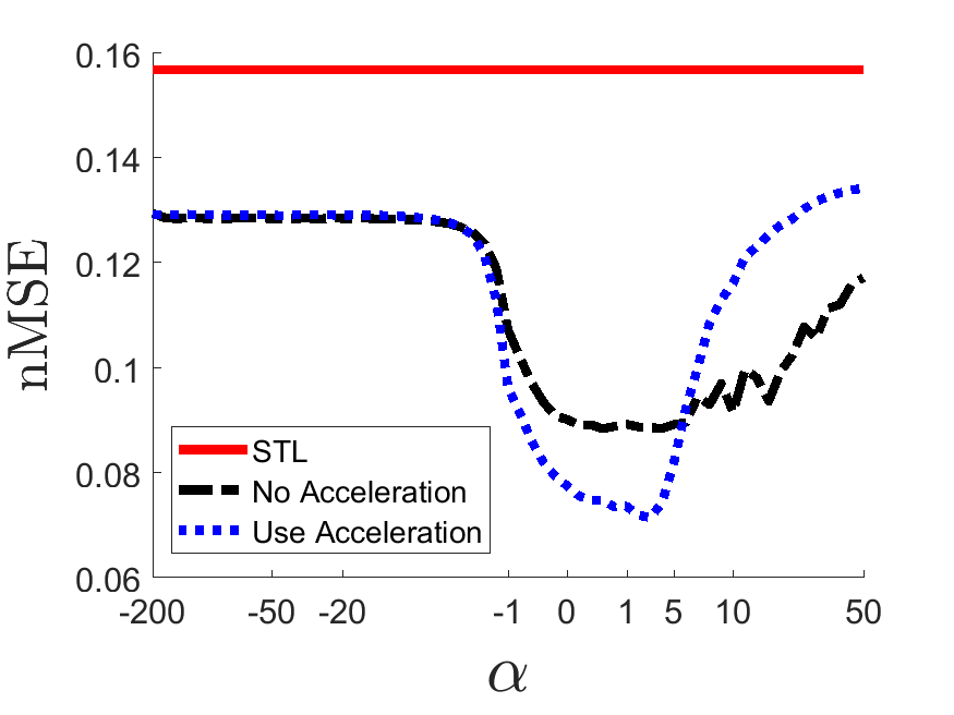
Refer to caption
(a) Convexity
Refer to caption
(b) Strong convexity
Figure 4: Evaluations for privacy-budget allocation strategies. In (a), we set ϵt=Θ(tα)subscriptitalic-ϵ𝑡Θsuperscript𝑡𝛼\epsilon_{t}=\Theta(t^{\alpha}), for t[T]𝑡delimited-[]𝑇t\in[T]; in (b), we set ϵt=Θ(Qt)subscriptitalic-ϵ𝑡Θsuperscript𝑄𝑡\epsilon_{t}=\Theta(Q^{-t}), for t[T]𝑡delimited-[]𝑇t\in[T]. Q0=1μ0.9684subscript𝑄01𝜇0.9684Q_{0}=1-\sqrt{\mu}\approx 0.9684. The results shown are averages of 100100100 runs with ϵ=0.1italic-ϵ0.1\epsilon=0.1. For the non-private MTL method, the nMSE was 0.01400.01400.0140.

5.4.2 Noise-to-Signal Ratio

Based on the setting in Section 5.4.1, the noise-to-signal ratios under the best privacy-budget allocation strategy (using acceleration and considering basic convexity) are shown in Fig. 5, in which we executed Algorithm 2 on the synthetic data set with the low-rank pattern. In contrast, for DP-MTRL, log10(𝐄F/𝚺~(t)F)=0.2670±0.0075subscript10subscriptnorm𝐄𝐹subscriptnormsuperscript~𝚺𝑡𝐹plus-or-minus0.26700.0075\log_{10}(\|\mathbf{E}\|_{F}/\|\widetilde{\mbox{\boldmath$\Sigma$}}^{(t)}\|_{F})=0.2670\pm 0.0075 under the best iteration number T=1𝑇1T=1. The output model matrices of DP-MTRL and our method are shown in Fig. 3 (e) and (f), and their respective covariance matrices are shown in Fig. 3 (b) and (c), respectively. These plots suggest that the high levels of noises added in our method had little influence on the output model matrix and the pattern in its covariance matrix, because our method adds noise only to the knowledge-sharing process and our method degrades to an STL method under high noise levels (as shown in Proposition 1). In contrast, in DP-MTRL, the output model matrix and the pattern in the covariance matrix are significantly affected or even destroyed because the noise was added directly to the model matrix, resulting in negative side-effects. This result may also have occurred because DP-MTRL is a local private learning algorithm, which needs a much larger m𝑚m to achieve acceptable utility (see the discussion in Section 2.2).
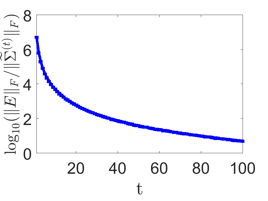
Refer to caption
Figure 5: Noise-to-signal ratios over the iterations of Algorithm 2. The results shown are averages of 100100100 runs with ϵ=0.1italic-ϵ0.1\epsilon=0.1.

5.4.3 Privacy-Accuracy Tradeoff

In Fig. 6, the performances of both of our MP-MTL algorithms (i.e., Algorithms 2 and 3) fall between those of the non-private STL and non-private MTL methods, suggesting that our methods are useful as MTL methods but may be affected by the introduced noise. In Fig. 6 (a), Algorithm 3 underperforms compared with Algorithm 2, because the true model matrix is not group-sparse. DP-MTRL outperforms the STL method and our Algorithm 3 when ϵitalic-ϵ\epsilon is large because it suits the true model matrix, in which the relatedness among tasks is modeled by a graph. In Fig. 6 (b), the true model matrix is group-sparse and is not suitable for DP-MTRL; hence, DP-MTRL underperforms compared with the STL method even when ϵitalic-ϵ\epsilon is large. Algorithm 2 rivals Algorithm 3 because the true model matrix is also low-rank. In both panels of Fig. 6, Algorithm 2 rivals the non-private MTL when ϵ=10italic-ϵ10\epsilon=10.

Refer to caption
(a) Low-rank pattern
Refer to caption
(b) Group-sparse pattern
Figure 6: Privacy-accuracy tradeoff on synthetic datasets. For (a), the data associated with the low-rank model matrix were used; for (b), the data associated with the group-sparse model matrix were used. MP-MTL-LR denotes Algorithm 2, MP-MTL-GS denotes Algorithm 3, and STL denotes the 2subscript2\ell_{2}-norm-penalized STL method. In both panels, STL and MTL denote non-private methods. In (b), the nMSEs of DP-MTRL are above 0.160.160.16; in both panels, the nMSEs of DP-AGGR are above 0.780.780.78. More detailed performances of DP-MTRL and DP-AGGR are presented in Fig. 7.

Fig. 7 shows the detailed performances for DP-MTRL and DP-AGGR corresponding to those in Fig. 6. Fig. 7 (c) is used to show that the accuracy of DP-AGGR grows with ϵitalic-ϵ\epsilon under the same setting as in Fig. 7 (b). As discussed previously, DP-AGGR performs only model averaging, which is not suitable for the true model matrices in both settings of Fig. 7 (a) and (b); hence, the accuracies of DP-AGGR are much worse than those of the respective STL methods.
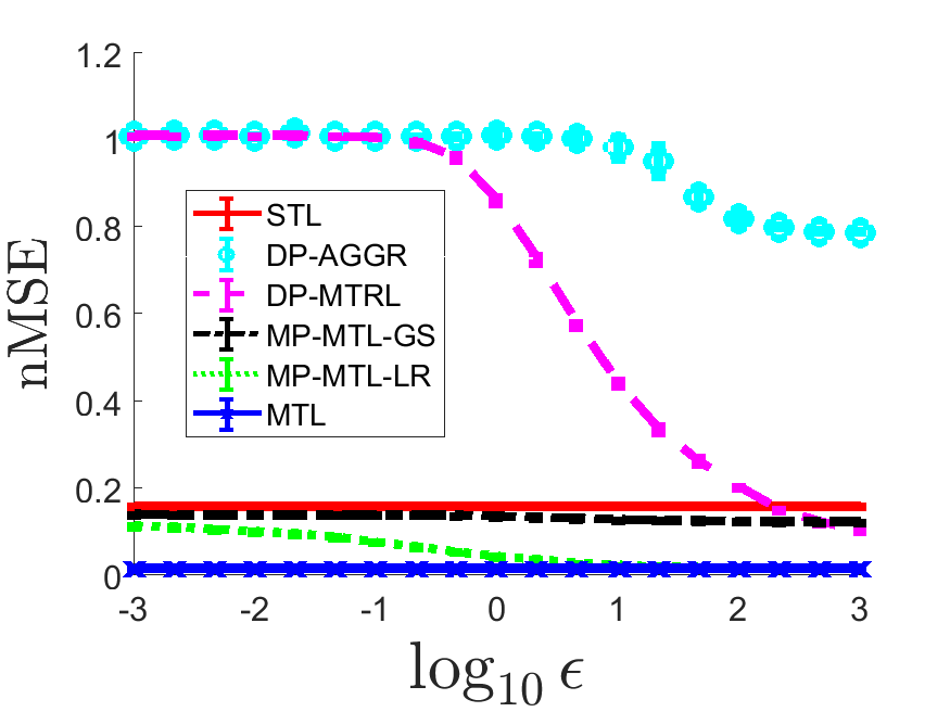
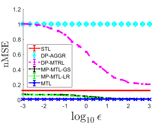
Refer to caption
(a) Low-rank pattern
Refer to caption
(b) Group-sparse pattern
Refer to caption
(c) Group-sparse pattern
Figure 7: Detailed privacy-accuracy tradeoff on synthetic datasets for DP-MTRL and DP-AGGR. For (a), the data associated with the low-rank model matrix were used; for (b) and (c), the data that associated with the group-sparse model matrix were used. In (c), the plot shows the same performances of DP-AGGR as those in (b) but with a finer vertical axis. Other settings are the same as those used for Fig. 6.

5.4.4 Varing the Number of Tasks

Based on the setting in Section 5.4.1, the average performances of the first 202020 of the 320320320 total tasks are shown in Fig. 8 under different numbers of training tasks. The accuracy increases with the number of tasks involved, which is consistent with our utility analyses. The standard deviation of each result is plotted in Fig. 8, showing that the increments are statistically significant.
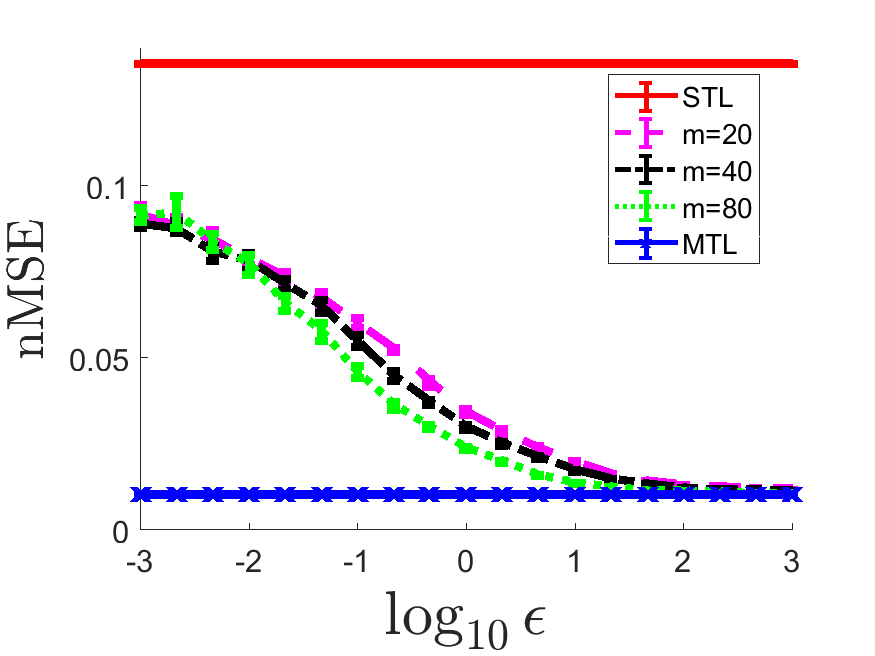
Refer to caption
Figure 8: Behaviors based on the number of tasks m𝑚m used for training. We used 320320320 tasks for MTL training.

5.5 Application

5.5.1 Data Description

We also evaluate the considered methods on the following two real datasets.

School Data. The School dataset111http://www.cs.ucl.ac.uk/staff/a.argyriou/code/ is a popular dataset for MTL [30] that consists of the exam scores of 15,362 students from 139 secondary schools. Each student is described by 27 attributes, including both school-specific information and student-specific information such as gender and ethnic group. The problem of predicting exam scores for the students can be formulated as an MTL problem: the number of tasks is m=139𝑚139m=139, the data dimensionality is d=27𝑑27d=27, and the number of data samples is ini=15,362subscript𝑖subscript𝑛𝑖15362\sum_{i}n_{i}=15,362.

LSOA II Data. These data are from the Second Longitudinal Study of Aging (LSOA II) 222https://www.cdc.gov/nchs/lsoa/lsoa2.htm.. LSOA II was a collaborative study conducted by the National Center for Health Statistics (NCHS) and the National Institute of Aging from 1994 to 2000. A national representative sample of 9,44794479,447 subjects of 707070 years of age and older were selected and interviewed. Three separate interviews were conducted with each subject, one each during the periods of 1994–1996, 1997–1998, and 1999–2000, referred to as WAVE 1, WAVE 2, and WAVE 3, respectively. Each wave of interviews included multiple modules covering a wide range of assessments. We used data from WAVE 2 and WAVE 3, which include a total of 4,29942994,299 sample subjects and 44 targets (each subject corresponded to 44 targets). We extracted 188188188 features from the WAVE 2 interviews. The targets include m=41𝑚41m=41 binary outcomes used in this study. These outcomes fall into several categories: 7 measures of fundamental daily activity, 13 of extended daily activity, 5 of social involvement, 8 of medical condition, 4 of cognitive ability, and 4 of sensation condition.

The features include demographic, family structure, daily personal care, medical history, social activity, health opinions, behavior, nutrition, health insurance and income and asset attributes, the majority of which are binary values.

Both the targets and the features have missing values due to non-responsed and questionnaire filtering. The average missing value rates of the targets and features are 13.7% and 20.2%, respectively. To address the missing values among the features, we adopted the following preprocessing procedure. For the continuous features, missing values were imputed with the sample mean. For binary features, it is better to treat the missing values as a third category because the absence of a value may also carry important information. Therefore, two dummy variables were created for each binary feature with missing values (no third variable is necessary in such a case) resulting in a total of d=295𝑑295d=295 features. To address the missing values among the targets, we included the samples associated with the observed targets for each task, resulting in maxi[m]ni=3,473subscript𝑖delimited-[]𝑚subscript𝑛𝑖3473\max_{i\in[m]}n_{i}=3,473.

For both the real-world datasets, We randomly selected 30% of the samples from each task to form the training set and used the remaining samples as the test set. For all the tasks, each data point was normalized to have a unit length.

5.5.2 Privacy-Accuracy Tradeoff

From Fig. 9, we can observe results similar to those seen in Fig. 6. In addition, our MP-MTL algorithms outperform the baseline MP-MTL methods, DP-MTRL and DP-AGGR, especially when ϵitalic-ϵ\epsilon is small. DP-AGGR underperforms compared with the STL method because its model averaging approach assumes that the tasks are homogeneous. In Fig. 9 (b), the aAUC values of DP-MTRL and our Algorithms (2 and 3) increase slowly because the feature dimension is large and the number of tasks is insufficient, which is consistent with our utility analyses.
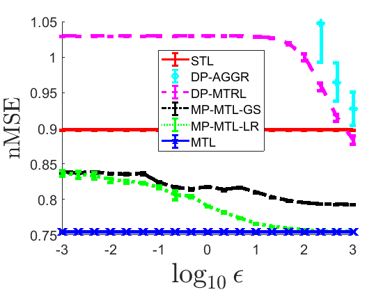
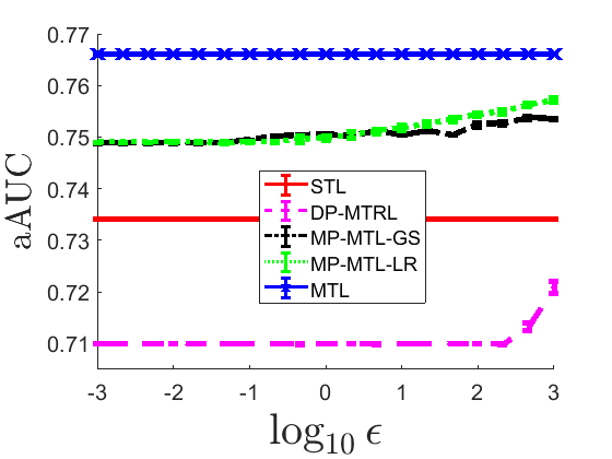
Refer to caption
(a) School Data
Refer to caption
(b) LSOA II Data
Figure 9: Privacy-accuracy tradeoff on real-world datasets. In both panels, MTL denotes the method with the best performance among the four non-private MTL methods proposed by Ji and Ye [39]Liu et al. [49]Zhang and Yeung [77] and DP-AGGR without perturbations; MP-MTL-LR denotes Algorithm 2, whereas MP-MTL-GS denotes Algorithm 3; STL denotes the method with the better performance between the 1subscript1\ell_{1}- and 2subscript2\ell_{2}-regularized methods. In (b), the aAUCs of DP-AGGR are below 0.660.660.66. The detailed performances of DP-AGGR are presented in Fig. 10.

Fig. 10 shows the detailed performances of DP-AGGR. In Fig. 10 (b), because the dimension is large and the number of tasks is insufficient, the accuracy of DP-AGGR barely grows with ϵitalic-ϵ\epsilon.

Refer to caption
(a) School Data
Refer to caption
(b) LSOA II Data
Figure 10: Detailed privacy-accuracy tradeoff on real-world datasets for DP-AGGR. All the settings are the same as those in Fig. 9.

Because the MTL behavior may change when the training-data percentage (the size of the training data divided by the size of the entire dataset) changes, we evaluated the methods on both real-world datasets at different training-data percentages and achieved similar results; see the supplementary material for more details.

6 Conclusions

In this paper, we discussed the potential security risks of multi-task learning approaches and presented a rigorous mathematical formulation of the model-protected multi-task learning (MP-MTL) problem. We proposed an algorithmic framework for implementing MP-MTL along with two concrete framework instantiations that learn the low-rank and group-sparse patterns in the model matrix. We demonstrated that our algorithms are guaranteed not to underperform compared with single-task learning methods under high noise levels. Privacy guarantees were provided. The utility analyses suggested that both the strong-convexity condition and the acceleration strategy improve the utility bounds, and that the acceleration strategy also improves the runtime. A utility analysis for privacy-budget allocation yielded a recommendation for privacy budgets that are non-decreasing over the iterations. The experiments demonstrated that our algorithms significantly outperform baseline methods constructed by existing privacy-preserving MTL methods on the proposed model-protection problem. Some interesting future research directions include developing concrete MP-MTL algorithms for other MTL approaches and other optimization schemes.

Acknowledgments

This research was supported in part by the National Science Foundation (NSF) under grants IIS-1565596, III-1615597 and IIS-1650723, in part by the Office of Naval Research (ONR) under grant number N00014-14-1-0631, and in part by the National Institutes of Health (NIH) under grants R00LM011392 and R21LM012060. In addition, we would like to thank Yuxiang Wang from the School of Computer Science at Carnegie Mellon University for his valuable comments on how to improve the properties of iterative MP-MTL algorithms.

References

  • Abadi et al. [2016] M. Abadi, A. Chu, I. Goodfellow, H. B. McMahan, I. Mironov, K. Talwar, and L. Zhang. Deep learning with differential privacy. In Proceedings of the 2016 ACM SIGSAC Conference on Computer and Communications Security, pages 308–318. ACM, 2016.
  • Almeida and Martins [2013] M. B. Almeida and A. F. Martins. Fast and robust compressive summarization with dual decomposition and multi-task learning. In ACL (1), pages 196–206, 2013.
  • Amit et al. [2007] Y. Amit, M. Fink, N. Srebro, and S. Ullman. Uncovering shared structures in multiclass classification. In Proceedings of the 24th ICML, pages 17–24, 2007.
  • Ando and Zhang [2005] R. K. Ando and T. Zhang. A framework for learning predictive structures from multiple tasks and unlabeled data. The Journal of Machine Learning Research, 6:1817–1853, 2005.
  • Apostol [1999] T. M. Apostol. An elementary view of euler’s summation formula. The American Mathematical Monthly, 106(5):409–418, 1999.
  • Argyriou et al. [2007a] A. Argyriou, T. Evgeniou, and M. Pontil. Multi-task feature learning. Advances in neural information processing systems, 19:41, 2007a.
  • Argyriou et al. [2007b] A. Argyriou, M. Pontil, Y. Ying, and C. A. Micchelli. A spectral regularization framework for multi-task structure learning. In Advances in Neural Information Processing Systems, pages 25–32, 2007b.
  • Argyriou et al. [2008] A. Argyriou, T. Evgeniou, and M. Pontil. Convex multi-task feature learning. Machine Learning, 73(3):243–272, 2008.
  • Barak et al. [2007] B. Barak, K. Chaudhuri, C. Dwork, S. Kale, F. McSherry, and K. Talwar. Privacy, Accuracy, and Consistency Too: A Holistic Solution to Contingency Table Release. In Proceedings of the 26th ACM SIGMOD-SIGACT-SIGART Symposium on Principles of Database Systems (PODS), pages 273–282, 2007.
  • Baytas et al. [2016] I. M. Baytas, M. Yan, A. K. Jain, and J. Zhou. Asynchronous multi-task learning. In Data Mining (ICDM), 2016 IEEE 16th International Conference on, pages 11–20. IEEE, 2016.
  • Blocki et al. [2012] J. Blocki, A. Blum, A. Datta, and O. Sheffet. The johnson-lindenstrauss transform itself preserves differential privacy. In Foundations of Computer Science (FOCS), 2012 IEEE 53rd Annual Symposium on, pages 410–419. IEEE, 2012.
  • Bonilla et al. [2007] E. V. Bonilla, K. M. A. Chai, and C. K. Williams. Multi-task gaussian process prediction. In NIPs, volume 20, pages 153–160, 2007.
  • Caruana [1997] R. Caruana. Multitask learning. Machine learning, 28(1):41–75, 1997.
  • Chan et al. [2011] T.-H. H. Chan, E. Shi, and D. Song. Private and continual release of statistics. ACM Transactions on Information and System Security (TISSEC), 14(3):26, 2011.
  • Chaudhuri and Monteleoni [2008] K. Chaudhuri and C. Monteleoni. Privacy-preserving logistic regression. In Advances in Neural Information Processing Systems, pages 289–296, 2008.
  • Chaudhuri et al. [2011a] K. Chaudhuri, C. Monteleoni, and A. Sarwate. Differentially Private Empirical Risk Minimization. Journal of Machine Learning Research (JMLR), 12:1069–1109, jul 2011a.
  • Chaudhuri et al. [2011b] K. Chaudhuri, C. Monteleoni, and A. D. Sarwate. Differentially private empirical risk minimization. The Journal of Machine Learning Research, 12:1069–1109, 2011b.
  • Chen et al. [2009] J. Chen, L. Tang, J. Liu, and J. Ye. A convex formulation for learning shared structures from multiple tasks. In Proceedings of the 26th ICML, pages 137–144, 2009.
  • Chen et al. [2011] J. Chen, J. Zhou, and J. Ye. Integrating low-rank and group-sparse structures for robust multi-task learning. In Proceedings of the 17th ACM SIGKDD Conference, pages 42–50. ACM, 2011.
  • Chen et al. [2012] J. Chen, J. Liu, and J. Ye. Learning incoherent sparse and low-rank patterns from multiple tasks. ACM Transactions on Knowledge Discovery from Data (TKDD), 5(4):22, 2012.
  • Dwork et al. [2006] C. Dwork, F. McSherry, K. Nissim, and A. Smith. Calibrating noise to sensitivity in private data analysis. In Theory of Cryptography Conference, pages 265–284. Springer, 2006.
  • Dwork et al. [2010] C. Dwork, M. Naor, T. Pitassi, and G. N. Rothblum. Differential privacy under continual observation. In Proceedings of the forty-second ACM symposium on Theory of computing, pages 715–724. ACM, 2010.
  • Dwork et al. [2014a] C. Dwork, A. Roth, et al. The algorithmic foundations of differential privacy. Foundations and Trends® in Theoretical Computer Science, 9(3–4):211–407, 2014a.
  • Dwork et al. [2014b] C. Dwork, K. Talwar, A. Thakurta, and L. Zhang. Analyze gauss: optimal bounds for privacy-preserving principal component analysis. In Proceedings of the 46th Annual ACM Symposium on Theory of Computing, pages 11–20. ACM, 2014b.
  • Evgeniou and Pontil [2007] A. Evgeniou and M. Pontil. Multi-task feature learning. In Advances in neural information processing systems, volume 19, page 41. The MIT Press, 2007.
  • Fei and Huan [2013] H. Fei and J. Huan. Structured feature selection and task relationship inference for multi-task learning. Knowledge and information systems, 35(2):345–364, 2013.
  • Finlayson et al. [2019] S. G. Finlayson, J. D. Bowers, J. Ito, J. L. Zittrain, A. L. Beam, and I. S. Kohane. Adversarial attacks on medical machine learning. Science, 363(6433):1287–1289, 2019.
  • Ganta et al. [2008] S. R. Ganta, S. P. Kasiviswanathan, and A. Smith. Composition attacks and auxiliary information in data privacy. In Proceedings of the 14th ACM SIGKDD Conference, pages 265–273. ACM, 2008.
  • Goldreich [1998] O. Goldreich. Secure multi-party computation. Manuscript. Preliminary version, pages 86–97, 1998.
  • Gong et al. [2012] P. Gong, J. Ye, and C. Zhang. Robust multi-task feature learning. In Proceedings of the 18th ACM SIGKDD Conference, pages 895–903. ACM, 2012.
  • Gu and Zhou [2009] Q. Gu and J. Zhou. Learning the shared subspace for multi-task clustering and transductive transfer classification. In Proceedings of ICDM, pages 159–168. IEEE, 2009.
  • Gu et al. [2016] Q. Gu, Z. Wang, and H. Liu. Low-rank and sparse structure pursuit via alternating minimization. In AISTATS, volume 51, pages 600–609, 2016.
  • Gupta and Nagar [1999] A. K. Gupta and D. K. Nagar. Matrix variate distributions, volume 104. CRC Press, 1999.
  • Gupta et al. [2016] S. K. Gupta, S. Rana, and S. Venkatesh. Differentially private multi-task learning. In Pacific-Asia Workshop on Intelligence and Security Informatics, pages 101–113. Springer, 2016.
  • Han and Zhang [2016] L. Han and Y. Zhang. Multi-stage multi-task learning with reduced rank. In Thirtieth AAAI Conference on Artificial Intelligence, 2016.
  • Hsu et al. [2013] J. Hsu, A. Roth, and J. Ullman. Differential privacy for the analyst via private equilibrium computation. In Proceedings of the forty-fifth annual ACM symposium on Theory of computing, pages 341–350. ACM, 2013.
  • Jaggi [2013] M. Jaggi. Revisiting frank-wolfe: Projection-free sparse convex optimization. In ICML (1), pages 427–435, 2013.
  • Jalali et al. [2010] A. Jalali, S. Sanghavi, C. Ruan, and P. K. Ravikumar. A dirty model for multi-task learning. In Advances in Neural Information Processing Systems, pages 964–972, 2010.
  • Ji and Ye [2009] S. Ji and J. Ye. An accelerated gradient method for trace norm minimization. In Proceedings of the 26th annual international conference on machine learning, pages 457–464. ACM, 2009.
  • Ji et al. [2014] Z. Ji, X. Jiang, H. Li, L. Xiong, and L. Ohno-Machado. Select and Label (S & L): a Task-Driven Privacy-Preserving Data Synthesization Framework. In Translational Bioinformatics Conference (TBC), Qingdao, China, 2014.
  • Jiang et al. [2016] W. Jiang, C. Xie, and Z. Zhang. Wishart mechanism for differentially private principal components analysis. In Thirtieth AAAI Conference on Artificial Intelligence, 2016.
  • Kairouz et al. [2017] P. Kairouz, S. Oh, and P. Viswanath. The composition theorem for differential privacy. IEEE Transactions on Information Theory, 2017.
  • Kasiviswanathan et al. [2011] S. P. Kasiviswanathan, H. K. Lee, K. Nissim, S. Raskhodnikova, and A. Smith. What can we learn privately? SIAM Journal on Computing, 40(3):793–826, 2011.
  • Kearns et al. [2014] M. Kearns, M. Pai, A. Roth, and J. Ullman. Mechanism design in large games: Incentives and privacy. In Proceedings of the 5th conference on Innovations in theoretical computer science, pages 403–410. ACM, 2014.
  • Kearns et al. [2015] M. Kearns, M. M. Pai, R. Rogers, A. Roth, and J. Ullman. Robust mediators in large games. arXiv preprint arXiv:1512.02698, 2015.
  • Kurakin et al. [2016] A. Kurakin, I. Goodfellow, and S. Bengio. Adversarial examples in the physical world. arXiv preprint arXiv:1607.02533, 2016.
  • Li et al. [2014] H. Li, L. Xiong, and X. Jiang. Differentially Private Synthesization of Multi-Dimensional Data using Copula Functions. In 17th International Conference on Extending Database Technology (EDBT 2014), Athens, Greece, 2014.
  • Li et al. [2010] J. Li, Y. Tian, T. Huang, and W. Gao. Probabilistic multi-task learning for visual saliency estimation in video. International Journal of Computer Vision, 90(2):150–165, 2010.
  • Liu et al. [2009] J. Liu, S. Ji, and J. Ye. Multi-task feature learning via efficient l 2, 1-norm minimization. In Proceedings of the twenty-fifth conference on uncertainty in artificial intelligence, pages 339–348. AUAI Press, 2009.
  • Mathew and Obradovic [2012] G. Mathew and Z. Obradovic. Distributed privacy preserving decision support system for predicting hospitalization risk in hospitals with insufficient data. In Machine Learning and Applications (ICMLA), 2012 11th International Conference on, volume 2, pages 178–183. IEEE, 2012.
  • Moosavi-Dezfooli et al. [2016] S.-M. Moosavi-Dezfooli, A. Fawzi, and P. Frossard. Deepfool: a simple and accurate method to fool deep neural networks. In Proceedings of the IEEE Conference on Computer Vision and Pattern Recognition, pages 2574–2582, 2016.
  • Mopuri et al. [2017] K. R. Mopuri, U. Garg, and R. V. Babu. Fast feature fool: A data independent approach to universal adversarial perturbations. arXiv preprint arXiv:1707.05572, 2017.
  • Ng et al. [2015] K. Ng, J. Sun, J. Hu, and F. Wang. Personalized predictive modeling and risk factor identification using patient similarity. AMIA Summits on Translational Science Proceedings, 2015:132, 2015.
  • Nie et al. [2010] F. Nie, H. Huang, X. Cai, and C. H. Ding. Efficient and robust feature selection via joint ℓ2, 1-norms minimization. In Advances in neural information processing systems, pages 1813–1821, 2010.
  • Nissim et al. [2007] K. Nissim, S. Raskhodnikova, and A. Smith. Smooth sensitivity and sampling in private data analysis. In Proceedings of the thirty-ninth annual ACM symposium on Theory of computing, pages 75–84. ACM, 2007.
  • Papernot et al. [2016a] N. Papernot, P. McDaniel, and I. Goodfellow. Transferability in machine learning: from phenomena to black-box attacks using adversarial samples. arXiv preprint arXiv:1605.07277, 2016a.
  • Papernot et al. [2016b] N. Papernot, P. McDaniel, I. Goodfellow, S. Jha, Z. B. Celik, and A. Swami. Practical black-box attacks against deep learning systems using adversarial examples. arXiv preprint arXiv:1602.02697, 2016b.
  • Pathak et al. [2010] M. Pathak, S. Rane, and B. Raj. Multiparty differential privacy via aggregation of locally trained classifiers. In Advances in Neural Information Processing Systems, pages 1876–1884, 2010.
  • Pong et al. [2010] T. K. Pong, P. Tseng, S. Ji, and J. Ye. Trace norm regularization: reformulations, algorithms, and multi-task learning. SIAM Journal on Optimization, 20(6):3465–3489, 2010.
  • Schmidt et al. [2011] M. Schmidt, N. L. Roux, and F. R. Bach. Convergence rates of inexact proximal-gradient methods for convex optimization. In Advances in neural information processing systems, pages 1458–1466, 2011.
  • Shokri and Shmatikov [2015] R. Shokri and V. Shmatikov. Privacy-preserving deep learning. In Proceedings of the 22nd ACM SIGSAC conference on computer and communications security, pages 1310–1321. ACM, 2015.
  • Song et al. [2013] S. Song, K. Chaudhuri, and A. D. Sarwate. Stochastic gradient descent with differentially private updates. In 2013 IEEE Global Conference on Signal and Information Processing, pages 245–248. IEEE, dec 2013. ISBN 978-1-4799-0248-4. doi: 10.1109/GlobalSIP.2013.6736861.
  • Su et al. [2018] C. Su, F. Yang, S. Zhang, Q. Tian, L. S. Davis, and W. Gao. Multi-task learning with low rank attribute embedding for multi-camera person re-identification. IEEE transactions on pattern analysis and machine intelligence, 40(5):1167–1181, 2018.
  • Sun et al. [2015] Z. Sun, F. Wang, and J. Hu. Linkage: An approach for comprehensive risk prediction for care management. In Proceedings of the 21th ACM SIGKDD Conference, pages 1145–1154. ACM, 2015.
  • Szegedy et al. [2013] C. Szegedy, W. Zaremba, I. Sutskever, J. Bruna, D. Erhan, I. Goodfellow, and R. Fergus. Intriguing properties of neural networks. arXiv preprint arXiv:1312.6199, 2013.
  • Turlach et al. [2005] B. A. Turlach, W. N. Venables, and S. J. Wright. Simultaneous variable selection. Technometrics, 47(3):349–363, 2005.
  • Vadhan [2016] S. Vadhan. The complexity of differential privacy. Work. Pap., Cent. Res. Comput. Soc., Harvard Univ. http://privacytools. seas. harvard. edu/publications/complexity-differential-privacy, 2016.
  • Wang et al. [2014] X. Wang, F. Wang, J. Hu, and R. Sorrentino. Exploring joint disease risk prediction. In AMIA Annual Symposium Proceedings, volume 2014, page 1180. American Medical Informatics Association, 2014.
  • Wang et al. [2015] Y.-X. Wang, S. Fienberg, and A. Smola. Privacy for Free: Posterior Sampling and Stochastic Gradient Monte Carlo. In Proceedings of the 32nd International Conference on Machine Learning (ICML-15), pages 2493–2502, 2015.
  • Wright et al. [2009] S. J. Wright, R. D. Nowak, and M. A. Figueiredo. Sparse reconstruction by separable approximation. IEEE Transactions on Signal Processing, 57(7):2479–2493, 2009.
  • Xu and Lafferty [2012] M. Xu and J. D. Lafferty. Conditional sparse coding and grouped multivariate regression. In Proceedings of the 29th ICML, pages 1479–1486, 2012.
  • Zantedeschi et al. [2017] V. Zantedeschi, M.-I. Nicolae, and A. Rawat. Efficient defenses against adversarial attacks. arXiv preprint arXiv:1707.06728, 2017.
  • Zhang et al. [2012a] J. Zhang, Z. Zhang, X. Xiao, Y. Yang, and M. Winslett. Functional mechanism. Proceedings of the VLDB Endowment, 5(11):1364–1375, jul 2012a. ISSN 21508097. doi: 10.14778/2350229.2350253.
  • Zhang et al. [2014] P. Zhang, F. Wang, J. Hu, and R. Sorrentino. Towards personalized medicine: leveraging patient similarity and drug similarity analytics. AMIA Summits on Translational Science Proceedings, 2014:132, 2014.
  • Zhang et al. [2012b] T. Zhang, B. Ghanem, S. Liu, and N. Ahuja. Robust visual tracking via multi-task sparse learning. In IEEE CVPR Conference, pages 2042–2049. IEEE, 2012b.
  • Zhang and Yang [2017] Y. Zhang and Q. Yang. A survey on multi-task learning. arXiv preprint arXiv:1707.08114, 2017.
  • Zhang and Yeung [2010] Y. Zhang and D.-Y. Yeung. A convex formulation for learning task relationships in multi-task learning. In Proceedings of the Twenty-Sixth Conference on Uncertainty in Artificial Intelligence, pages 733–742. AUAI Press, 2010.
  • Zhen et al. [2018] X. Zhen, M. Yu, X. He, and S. Li. Multi-target regression via robust low-rank learning. IEEE transactions on pattern analysis and machine intelligence, 40(2):497–504, 2018.
  • Zhou et al. [2011] J. Zhou, J. Chen, and J. Ye. Clustered multi-task learning via alternating structure optimization. In Advances in neural information processing systems, pages 702–710, 2011.
[Uncaptioned image] Jian Liang received his B.S. degree in automation from the Huazhong University of Science and Technology, Wuhan, China, in 2012. He is currently working toward his Ph.D. degree in the Department of Automation at Tsinghua University, Beijing. His research interests lie in the areas of multi-task learning and time-series data mining. He won the Best Short Paper Award at the 2016 IEEE International Conference on Healthcare Informatics (ICHI).
[Uncaptioned image] Ziqi Liu Ziqi Liu is currently a Ph.D. student at Xi’an Jiaotong University under advisor Professor Qinghua Zheng. His research interests lie in scalable machine learning and nonparametric modeling. The major awards he has received include the WSDM’16 Best Research Paper Award.
[Uncaptioned image] Jiayu Zhou Jiayu Zhou is currently an assistant professor in the Department of Computer Science and Engineering at Michigan State University. He received his Ph.D. degree in computer science from Arizona State University in 2014. He has broad research interests in the fields of large-scale machine learning and data mining as well as biomedical informatics. He has served as a technical program committee member for premier conferences such as NIPS, ICML, and SIGKDD. His papers have received the Best Student Paper Award at the 2014 IEEE International Conference on Data Mining (ICDM), the Best Student Paper Award at the 2016 International Symposium on Biomedical Imaging (ISBI) and the Best Paper Award at IEEE Big Data 2016.
[Uncaptioned image] Xiaoqian Jiang is an assistant professor in the Department of Biomedical Informatics at the University of California, San Diego. He received his Ph.D. in computer science from Carnegie Mellon University. He is an associate editor of BMC Medical Informatics and Decision Making and serves as a member of the editorial board of the Journal of the American Medical Informatics Association. He works primarily in the fields of health data privacy and predictive models in biomedicine. Dr. Jiang was a recipient of the NIH K99/R00 award and won the Distinguished Paper Award from the American Medical Informatics Association Clinical Research Informatics (CRI) Summit in 2012 and 2013.
[Uncaptioned image] Changshui Zhang received his B.S. degree from Peking University, Beijing, China, in 1986 and his Ph.D. degree from Tsinghua University, Beijing, China, in 1992. He is currently a professor in the Department of Automation at Tsinghua University. He is a member of the editorial board of Pattern Recognition and an IEEE Fellow. His research interests include artificial intelligence, image processing, pattern recognition, machine learning and evolutionary computation.
[Uncaptioned image] Fei Wang is an assistant professor in the Division of Health Informatics of the Department of Healthcare Policy and Research at Cornell University. His major research interest lies in data analytics and its applications in health informatics. His papers have received over 3,700 citations, with an H-index of 33. He won the Best Student Paper Award at ICDM 2015, received a Best Research Paper nomination at ICDM 2010, and the Marco Romani Best Paper nomination at AMIA TBI 2014, and his papers were selected as Best Paper finalists at SDM 2011 and 2015. Dr. Wang is an active editor of the journal Data Mining and Knowledge Discovery, an associate editor of the Journal of Health Informatics Research and Smart Health, and a member of the editorial boards of Pattern Recognition and the International Journal of Big Data and Analytics in Healthcare. Dr. Wang is also the vice chair of the KDD working group at AMIA.

Supplemental Materials: Model-Protected Multi-Task Learning

Appendix A Model-Decomposed MP-MTL Methods

In this section, we consider the extension of our MP-MTL framework for MTL methods using the decomposed parameter/model matrix. Specifically, we focus on the following problem, where the trace norm is used for knowledge sharing across tasks and the 1\|\cdot\|_{1} norm (sum of the 1subscript1\ell_{1} norm for vectors) is used for entry-wise outlier detection, as described in Algorithm 4.

min𝐖i=1mi(𝐗i𝐰i,𝐲i)+λ1𝐏+λ2𝐐1s.t.𝐖=𝐏+𝐐,formulae-sequencesubscript𝐖superscriptsubscript𝑖1𝑚subscript𝑖subscript𝐗𝑖subscript𝐰𝑖subscript𝐲𝑖subscript𝜆1subscriptdelimited-∥∥𝐏subscript𝜆2subscriptdelimited-∥∥𝐐1𝑠𝑡𝐖𝐏𝐐\begin{split}\min_{\mathbf{W}}\ &\sum\nolimits_{i=1}^{m}\mathcal{L}_{i}(\mathbf{X}_{i}\mathbf{w}_{i},\mathbf{y}_{i})+\lambda_{1}\|\mathbf{P}\|_{*}+\lambda_{2}\|\mathbf{Q}\|_{1}\\ s.t.\ &\mathbf{W}=\mathbf{P}+\mathbf{Q},\end{split} (23)

where 𝐏,𝐐d×m𝐏𝐐superscript𝑑𝑚\mathbf{P},\mathbf{Q}\in\mathbb{R}^{d\times m}.

Algorithm 4 Model-Protected low-rank and group-sparse (MP-LR-SP) Estimator
0:  Datasets (𝐗m,𝐲m)={(𝐗1,𝐲1),,(𝐗m,𝐲m)}superscript𝐗𝑚superscript𝐲𝑚subscript𝐗1subscript𝐲1subscript𝐗𝑚subscript𝐲𝑚(\mathbf{X}^{m},\mathbf{y}^{m})=\{(\mathbf{X}_{1},\mathbf{y}_{1}),\ldots,(\mathbf{X}_{m},\mathbf{y}_{m})\}, where i[m],𝐗ini×dformulae-sequencefor-all𝑖delimited-[]𝑚subscript𝐗𝑖superscriptsubscript𝑛𝑖𝑑\forall i\in[m],\ \mathbf{X}_{i}\in\mathbb{R}^{n_{i}\times d} and 𝐲ini×1subscript𝐲𝑖superscriptsubscript𝑛𝑖1\mathbf{y}_{i}\in\mathbb{R}^{n_{i}\times 1}. Privacy loss ϵ,δ0italic-ϵ𝛿0\epsilon,\delta\geq 0. Number of iterations T𝑇T. Step size η𝜂\eta. Regularization parameter λ1,λ2>0subscript𝜆1subscript𝜆20\lambda_{1},\lambda_{2}>0. Norm clipping parameter K>0𝐾0K>0. Acceleration parameters {βt}subscript𝛽𝑡\{\beta_{t}\}. Initial models of tasks 𝐖(0)superscript𝐖0\mathbf{W}^{(0)}.
0:  𝐖^(1:T)superscript^𝐖:1𝑇\widehat{\mathbf{W}}^{(1:T)} .
1:  Set {ϵt}subscriptitalic-ϵ𝑡\{\epsilon_{t}\} such that CB({ϵt},δ)ϵ𝐶𝐵subscriptitalic-ϵ𝑡𝛿italic-ϵCB(\{\epsilon_{t}\},\delta)\leq\epsilon, where CB({ϵt},δ)𝐶𝐵subscriptitalic-ϵ𝑡𝛿CB(\{\epsilon_{t}\},\delta) is the composition bound of {ϵt}subscriptitalic-ϵ𝑡\{\epsilon_{t}\}.
2:  Let 𝐏(0)=𝐐(0)=𝐐^(0)=𝐖(0)superscript𝐏0superscript𝐐0superscript^𝐐0superscript𝐖0\mathbf{P}^{(0)}=\mathbf{Q}^{(0)}=\widehat{\mathbf{Q}}^{(0)}=\mathbf{W}^{(0)}.
3:  for t=1:T:𝑡1𝑇t=1:T do
4:     Norm clipping: 𝐩~i(t1)=𝐩i(t1)/max(1,𝐩i(t1)2K)superscriptsubscript~𝐩𝑖𝑡1superscriptsubscript𝐩𝑖𝑡11subscriptnormsuperscriptsubscript𝐩𝑖𝑡12𝐾\tilde{\mathbf{p}}_{i}^{(t-1)}={\mathbf{p}}_{i}^{(t-1)}/\max(1,\frac{\|{\mathbf{p}}_{i}^{(t-1)}\|_{2}}{K}) for all i[m]𝑖delimited-[]𝑚i\in[m]. Let 𝐏^(0)=𝐏~(0)superscript^𝐏0superscript~𝐏0\widehat{\mathbf{P}}^{(0)}=\widetilde{\mathbf{P}}^{(0)}.
5:     𝚺~(t)=𝐏~(t1)(𝐏~(t1))Tsuperscript~𝚺𝑡superscript~𝐏𝑡1superscriptsuperscript~𝐏𝑡1T\widetilde{\mbox{\boldmath$\Sigma$}}^{(t)}=\widetilde{\mathbf{P}}^{(t-1)}(\widetilde{\mathbf{P}}^{(t-1)})^{\rm T}.
6:     𝚺(t)=𝚺~(t1)+𝐄superscript𝚺𝑡superscript~𝚺𝑡1𝐄\mbox{\boldmath$\Sigma$}^{(t)}=\widetilde{\mbox{\boldmath$\Sigma$}}^{(t-1)}+\mathbf{E}, where 𝐄Wd(d+1,K22ϵt𝐈d)similar-to𝐄subscript𝑊𝑑𝑑1superscript𝐾22subscriptitalic-ϵ𝑡subscript𝐈𝑑\mathbf{E}\sim W_{d}(d+1,\frac{K^{2}}{2\epsilon_{t}}\mathbf{I}_{d}) is a sample of the Wishart distribution.
7:     Perform SVD decomposition: 𝐔𝚲𝐔T=𝚺(t)𝐔𝚲superscript𝐔Tsuperscript𝚺𝑡\mathbf{U}\mbox{\boldmath$\Lambda$}\mathbf{U}^{\rm T}={\mbox{\boldmath$\Sigma$}}^{(t)}.
8:     Let 𝐒ηλ1subscript𝐒𝜂subscript𝜆1\mathbf{S}_{\eta\lambda_{1}} be a diagonal matrix and let 𝐒ηλ1,ii=max{0,1ηλ1/𝚲ii}subscript𝐒𝜂subscript𝜆1𝑖𝑖01𝜂subscript𝜆1subscript𝚲𝑖𝑖\mathbf{S}_{\eta\lambda_{1},ii}=\max\{0,1-\eta\lambda_{1}/\sqrt{\mbox{\boldmath$\Lambda$}_{ii}}\} for i=1,,min{d,m}𝑖1𝑑𝑚i=1,\ldots,\min\{d,m\}.
9:     𝐌(t)=𝐔𝐒ηλ1𝐔Tsuperscript𝐌𝑡subscript𝐔𝐒𝜂subscript𝜆1superscript𝐔T\mathbf{M}^{(t)}=\mathbf{U}\mathbf{S}_{\eta\lambda_{1}}\mathbf{U}^{\rm T}.
10:     Let 𝐩^i(t)=𝐌(t)𝐩~i(t1)superscriptsubscript^𝐩𝑖𝑡superscript𝐌𝑡superscriptsubscript~𝐩𝑖𝑡1\hat{\mathbf{p}}_{i}^{(t)}=\mathbf{M}^{(t)}\tilde{\mathbf{p}}_{i}^{(t-1)} for all i[m]𝑖delimited-[]𝑚i\in[m].
11:     Let 𝐪^i(t)=sign(𝐪i(t1))max{0,|𝐪i(t1)|ηλ2}superscriptsubscript^𝐪𝑖𝑡signsuperscriptsubscript𝐪𝑖𝑡10superscriptsubscript𝐪𝑖𝑡1𝜂subscript𝜆2\hat{\mathbf{q}}_{i}^{(t)}=\mbox{sign}(\mathbf{q}_{i}^{(t-1)})\circ\max\{0,|\mathbf{q}_{i}^{(t-1)}|-\eta\lambda_{2}\} for all i[m]𝑖delimited-[]𝑚i\in[m], where \circ denotes the entry-wise product.
12:     Let 𝐖^(t)=𝐏^(t)+𝐐^(t)superscript^𝐖𝑡superscript^𝐏𝑡superscript^𝐐𝑡\widehat{\mathbf{W}}^{(t)}=\widehat{\mathbf{P}}^{(t)}+\widehat{\mathbf{Q}}^{(t)}.
13:     Let 𝒛i,p(t)=𝐩^i(t)+βt(𝐩^i(t)𝐩^i(t1))superscriptsubscript𝒛𝑖𝑝𝑡superscriptsubscript^𝐩𝑖𝑡subscript𝛽𝑡superscriptsubscript^𝐩𝑖𝑡superscriptsubscript^𝐩𝑖𝑡1{\mbox{\boldmath$z$}}_{i,p}^{(t)}=\hat{\mathbf{p}}_{i}^{(t)}+\beta_{t}(\hat{\mathbf{p}}_{i}^{(t)}-\hat{\mathbf{p}}_{i}^{(t-1)}) for all i[m]𝑖delimited-[]𝑚i\in[m].
14:     Let 𝒛i,q(t)=𝐪^i(t)+βt(𝐪^i(t)𝐪^i(t1))superscriptsubscript𝒛𝑖𝑞𝑡superscriptsubscript^𝐪𝑖𝑡subscript𝛽𝑡superscriptsubscript^𝐪𝑖𝑡superscriptsubscript^𝐪𝑖𝑡1{\mbox{\boldmath$z$}}_{i,q}^{(t)}=\hat{\mathbf{q}}_{i}^{(t)}+\beta_{t}(\hat{\mathbf{q}}_{i}^{(t)}-\hat{\mathbf{q}}_{i}^{(t-1)}) for all i[m]𝑖delimited-[]𝑚i\in[m].
15:     𝐩i(t)=𝒛i,p(t)ηi(𝐗i(𝒛i,p(t)+𝒛i,q(t)),𝐲i)𝐩^i(t)superscriptsubscript𝐩𝑖𝑡superscriptsubscript𝒛𝑖𝑝𝑡𝜂subscript𝑖subscript𝐗𝑖superscriptsubscript𝒛𝑖𝑝𝑡superscriptsubscript𝒛𝑖𝑞𝑡subscript𝐲𝑖superscriptsubscript^𝐩𝑖𝑡{\mathbf{p}}_{i}^{(t)}={\mbox{\boldmath$z$}}_{i,p}^{(t)}-\eta\frac{\partial\mathcal{L}_{i}(\mathbf{X}_{i}({\mbox{\boldmath$z$}}_{i,p}^{(t)}+{\mbox{\boldmath$z$}}_{i,q}^{(t)}),\mathbf{y}_{i})}{\partial\hat{\mathbf{p}}_{i}^{(t)}} for all i[m]𝑖delimited-[]𝑚i\in[m].
16:     𝐪i(t)=𝒛i,q(t)ηi(𝐗i(𝒛i,p(t)+𝒛i,q(t)),𝐲i)𝐪^i(t)superscriptsubscript𝐪𝑖𝑡superscriptsubscript𝒛𝑖𝑞𝑡𝜂subscript𝑖subscript𝐗𝑖superscriptsubscript𝒛𝑖𝑝𝑡superscriptsubscript𝒛𝑖𝑞𝑡subscript𝐲𝑖superscriptsubscript^𝐪𝑖𝑡{\mathbf{q}}_{i}^{(t)}={\mbox{\boldmath$z$}}_{i,q}^{(t)}-\eta\frac{\partial\mathcal{L}_{i}(\mathbf{X}_{i}({\mbox{\boldmath$z$}}_{i,p}^{(t)}+{\mbox{\boldmath$z$}}_{i,q}^{(t)}),\mathbf{y}_{i})}{\partial\hat{\mathbf{q}}_{i}^{(t)}} for all i[m]𝑖delimited-[]𝑚i\in[m].
17:  end for

We note that in Algorithm 4, the role of 𝐏𝐏\mathbf{P} is the same as the role of 𝐖𝐖\mathbf{W} in Algorithm 2, and the additional procedures introduced to update 𝐐𝐐\mathbf{Q} are still STL algorithms. As such, we have the result in Corollary 2.

Corollary 2.

Algorithm 4 is an (ϵ,δ)italic-ϵ𝛿(\epsilon,\delta) MP-MTL algorithm.

Proof.

For simplicity, we omit the symbol \mathcal{B} to denote the input in the conditional events in some equations.

Use Corollary 1 and Theorem 1. Given t[T]𝑡delimited-[]𝑇t\in[T], the algorithm (𝐏~(t1),𝚺(1:t1))(𝐌(t),𝚺(t))superscript~𝐏𝑡1superscript𝚺:1𝑡1superscript𝐌𝑡superscript𝚺𝑡(\widetilde{\mathbf{P}}^{(t-1)},\mbox{\boldmath$\Sigma$}^{(1:t-1)})\rightarrow(\mathbf{M}^{(t)},\mbox{\boldmath$\Sigma$}^{(t)}) is an (ϵt,0)subscriptitalic-ϵ𝑡0(\epsilon_{t},0)-differentially private algorithm, where 𝐌(t)=𝐔𝐒ηλ𝐔Tsuperscript𝐌𝑡subscript𝐔𝐒𝜂𝜆superscript𝐔T\mathbf{M}^{(t)}=\mathbf{U}\mathbf{S}_{\eta\lambda}\mathbf{U}^{\rm T}.

Now, for all i[m]𝑖delimited-[]𝑚i\in[m], applying the Post-Processing immunity property (Property 1) for the mapping f:(𝐌(t),𝐩~[i](t1))𝐩^[i](t1):𝑓superscript𝐌𝑡superscriptsubscript~𝐩delimited-[]𝑖𝑡1superscriptsubscript^𝐩delimited-[]𝑖𝑡1f:(\mathbf{M}^{(t)},\tilde{\mathbf{p}}_{[-i]}^{(t-1)})\rightarrow\hat{\mathbf{p}}_{[-i]}^{(t-1)}, which does not touch any unperturbed sensitive information of the i𝑖i-th task, we have for any set 𝒮d×(m1)𝒮superscript𝑑𝑚1\mathcal{S}\subseteq\mathbb{R}^{d\times(m-1)} that

(𝐩^\displaystyle\mathbb{P}(\hat{\mathbf{p}} [i](t1)𝒮𝐏~(t1),𝚺(1:t1)){}_{[-i]}^{(t-1)}\in\mathcal{S}\mid\widetilde{\mathbf{P}}^{(t-1)},\mbox{\boldmath$\Sigma$}^{(1:t-1)})
\displaystyle\leq eϵt(𝐩^[i](t1)𝒮(𝐏~)(t1),𝚺(1:t1)),superscript𝑒subscriptitalic-ϵ𝑡superscriptsubscript^𝐩delimited-[]𝑖𝑡1conditional𝒮superscriptsuperscript~𝐏𝑡1superscript𝚺:1𝑡1\displaystyle e^{\epsilon_{t}}\mathbb{P}(\hat{\mathbf{p}}_{[-i]}^{(t-1)}\in\mathcal{S}\mid(\widetilde{\mathbf{P}}^{\prime})^{(t-1)},\mbox{\boldmath$\Sigma$}^{(1:t-1)}),

where 𝐏~(t1)superscript~𝐏𝑡1\widetilde{\mathbf{P}}^{(t-1)} and (𝐏~)(t1)superscriptsuperscript~𝐏𝑡1(\widetilde{\mathbf{P}}^{\prime})^{(t-1)} differ only in the i𝑖i-th column.

Then, because in the t𝑡t-th iteration the mapping 𝐐(t1)𝐐^(t1)superscript𝐐𝑡1superscript^𝐐𝑡1\mathbf{Q}^{(t-1)}\rightarrow\widehat{\mathbf{Q}}^{(t-1)} is a deterministic STL algorithm, we have for any set 𝒮d×(m1)𝒮superscript𝑑𝑚1\mathcal{S}\subseteq\mathbb{R}^{d\times(m-1)} that

(𝐪^\displaystyle\mathbb{P}(\hat{\mathbf{q}} [i](t1)𝒮𝐐(t1)){}_{[-i]}^{(t-1)}\in\mathcal{S}\mid\mathbf{Q}^{(t-1)})
=\displaystyle= (𝐪^[i](t1)𝒮𝐪[i](t1),𝐪i(t1))superscriptsubscript^𝐪delimited-[]𝑖𝑡1conditional𝒮superscriptsubscript𝐪delimited-[]𝑖𝑡1superscriptsubscript𝐪𝑖𝑡1\displaystyle\mathbb{P}(\hat{\mathbf{q}}_{[-i]}^{(t-1)}\in\mathcal{S}\mid\mathbf{q}_{[-i]}^{(t-1)},\mathbf{q}_{i}^{(t-1)})
=\displaystyle= (𝐪^[i](t1)𝒮𝐪[i](t1),(𝐪i)(t1))superscriptsubscript^𝐪delimited-[]𝑖𝑡1conditional𝒮superscriptsubscript𝐪delimited-[]𝑖𝑡1superscriptsubscriptsuperscript𝐪𝑖𝑡1\displaystyle\mathbb{P}(\hat{\mathbf{q}}_{[-i]}^{(t-1)}\in\mathcal{S}\mid\mathbf{q}_{[-i]}^{(t-1)},(\mathbf{q}^{\prime}_{i})^{(t-1)})
=\displaystyle= e0(𝐪^[i](t1)𝒮(𝐐)(t1))+0,superscript𝑒0superscriptsubscript^𝐪delimited-[]𝑖𝑡1conditional𝒮superscriptsuperscript𝐐𝑡10\displaystyle e^{0}\mathbb{P}(\hat{\mathbf{q}}_{[-i]}^{(t-1)}\in\mathcal{S}\mid(\mathbf{Q}^{\prime})^{(t-1)})+0,

where 𝐐(t1)superscript𝐐𝑡1\mathbf{Q}^{(t-1)} and (𝐐)(t1)superscriptsuperscript𝐐𝑡1(\mathbf{Q}^{\prime})^{(t-1)} differ only in the i𝑖i-th column.

Then applying Combination property (Property 3), we have for any set 𝒮d×(m1)×d×(m1)𝒮superscript𝑑𝑚1superscript𝑑𝑚1\mathcal{S}\subseteq\mathbb{R}^{d\times(m-1)}\times\mathbb{R}^{d\times(m-1)}

((𝐩^\displaystyle\mathbb{P}((\hat{\mathbf{p}} ,[i](t1)𝐪^[i](t1))𝒮𝐏(t1),𝚺(1:t1),𝐐(t1)){}_{[-i]}^{(t-1)},\hat{\mathbf{q}}_{[-i]}^{(t-1)})\in\mathcal{S}\mid\mathbf{P}^{(t-1)},\mbox{\boldmath$\Sigma$}^{(1:t-1)},\mathbf{Q}^{(t-1)})
\displaystyle\leq eϵt((𝐩^[i](t1),𝐪^[i](t1))𝒮(𝐏)(t1),𝚺(1:t1),(𝐐)(t1)),superscript𝑒subscriptitalic-ϵ𝑡superscriptsubscript^𝐩delimited-[]𝑖𝑡1superscriptsubscript^𝐪delimited-[]𝑖𝑡1conditional𝒮superscriptsuperscript𝐏𝑡1superscript𝚺:1𝑡1superscriptsuperscript𝐐𝑡1\displaystyle e^{\epsilon_{t}}\mathbb{P}((\hat{\mathbf{p}}_{[-i]}^{(t-1)},\hat{\mathbf{q}}_{[-i]}^{(t-1)})\in\mathcal{S}\mid(\mathbf{P}^{\prime})^{(t-1)},\mbox{\boldmath$\Sigma$}^{(1:t-1)},(\mathbf{Q}^{\prime})^{(t-1)}),

Because the mapping(𝐏^(t1),𝐐^(t1),𝒟m)(𝐏^(t),𝐐^(t))superscript^𝐏𝑡1superscript^𝐐𝑡1superscript𝒟𝑚superscript^𝐏𝑡superscript^𝐐𝑡(\widehat{\mathbf{P}}^{(t-1)},\widehat{\mathbf{Q}}^{(t-1)},\mathcal{D}^{m})\rightarrow(\widehat{\mathbf{P}}^{(t)},\widehat{\mathbf{Q}}^{(t)}) is a deterministic STL algorithm, applying the Post-Processing immunity property (Property 1), we further have for any set 𝒮d×(m1)×d×(m1)𝒮superscript𝑑𝑚1superscript𝑑𝑚1\mathcal{S}\subseteq\mathbb{R}^{d\times(m-1)}\times\mathbb{R}^{d\times(m-1)} that

(\displaystyle\mathbb{P}( (𝐩^[i](t),𝐪^[i](t))𝒮𝐏(t1),𝚺(1:t1),𝐐(t1),𝒟m)\displaystyle(\hat{\mathbf{p}}_{[-i]}^{(t)},\hat{\mathbf{q}}_{[-i]}^{(t)})\in\mathcal{S}\mid\mathbf{P}^{(t-1)},\mbox{\boldmath$\Sigma$}^{(1:t-1)},\mathbf{Q}^{(t-1)},\mathcal{D}^{m})
\displaystyle\leq eϵt((𝐩^[i](t),𝐪^[i](t))𝒮(𝐏)(t1),𝚺(1:t1),(𝐐)(t1),(𝒟)m),superscript𝑒subscriptitalic-ϵ𝑡superscriptsubscript^𝐩delimited-[]𝑖𝑡superscriptsubscript^𝐪delimited-[]𝑖𝑡conditional𝒮superscriptsuperscript𝐏𝑡1superscript𝚺:1𝑡1superscriptsuperscript𝐐𝑡1superscriptsuperscript𝒟𝑚\displaystyle e^{\epsilon_{t}}\mathbb{P}((\hat{\mathbf{p}}_{[-i]}^{(t)},\hat{\mathbf{q}}_{[-i]}^{(t)})\in\mathcal{S}\mid(\mathbf{P}^{\prime})^{(t-1)},\mbox{\boldmath$\Sigma$}^{(1:t-1)},(\mathbf{Q}^{\prime})^{(t-1)},(\mathcal{D}^{\prime})^{m}),

where (𝒟)msuperscriptsuperscript𝒟𝑚(\mathcal{D}^{\prime})^{m} differs from 𝒟msuperscript𝒟𝑚\mathcal{D}^{m} in the entire dataset of the i𝑖i-th task.

Now, using Theorem 1, for t=1,,T𝑡1𝑇t=1,\ldots,T, we again take the t𝑡t-th dataset 𝒟~t={(𝐩1(t1),𝐪1(t1),𝒟1),,(𝐩m(t1),𝐪m(t1)𝒟m)}subscript~𝒟𝑡superscriptsubscript𝐩1𝑡1superscriptsubscript𝐪1𝑡1subscript𝒟1superscriptsubscript𝐩𝑚𝑡1superscriptsubscript𝐪𝑚𝑡1subscript𝒟𝑚\widetilde{\mathcal{D}}_{t}=\{(\mathbf{p}_{1}^{(t-1)},\mathbf{q}_{1}^{(t-1)},\mathcal{D}_{1}),\ldots,(\mathbf{p}_{m}^{(t-1)},\mathbf{q}_{m}^{(t-1)}\mathcal{D}_{m})\} and denote ϑt,i=(𝐪^[i](t),𝐪^[i](t),𝐌(t),𝚺(t))𝒞t,isubscriptitalic-ϑ𝑡𝑖superscriptsubscript^𝐪delimited-[]𝑖𝑡superscriptsubscript^𝐪delimited-[]𝑖𝑡superscript𝐌𝑡superscript𝚺𝑡subscript𝒞𝑡𝑖\vartheta_{t,i}=(\hat{\mathbf{q}}_{[-i]}^{(t)},\hat{\mathbf{q}}_{[-i]}^{(t)},\mathbf{M}^{(t)},\mbox{\boldmath$\Sigma$}^{(t)})\in\mathcal{C}_{t,i}. Given the fact that 𝐏(t)=𝐏^(t)superscript𝐏𝑡superscript^𝐏𝑡\mathbf{P}^{(t)}=\widehat{\mathbf{P}}^{(t)} and 𝐐(t)=𝐐^(t)superscript𝐐𝑡superscript^𝐐𝑡\mathbf{Q}^{(t)}=\widehat{\mathbf{Q}}^{(t)} for all t[T]𝑡delimited-[]𝑇t\in[T], we have for any set 𝒮t,i𝒞t,isubscript𝒮𝑡𝑖subscript𝒞𝑡𝑖\mathcal{S}_{t,i}\subseteq\mathcal{C}_{t,i} that

(ϑ\displaystyle\mathbb{P}(\vartheta t,i𝒮t,i𝒟~t,ϑ1:t1){}_{t,i}\in\mathcal{S}_{t,i}\mid\widetilde{\mathcal{D}}_{t},\mbox{\boldmath$\vartheta$}_{1:t-1})
\displaystyle\leq eϵt(ϑt,i𝒮t,i𝒟~t,ϑ1:t1),superscript𝑒subscriptitalic-ϵ𝑡subscriptitalic-ϑ𝑡𝑖conditionalsubscript𝒮𝑡𝑖subscriptsuperscript~𝒟𝑡subscriptbold-italic-ϑ:1𝑡1\displaystyle e^{\epsilon_{t}}\mathbb{P}(\vartheta_{t,i}\in\mathcal{S}_{t,i}\mid\widetilde{\mathcal{D}}^{\prime}_{t},\mbox{\boldmath$\vartheta$}_{1:t-1}),

where 𝒟~tsubscript~𝒟𝑡\widetilde{\mathcal{D}}_{t} and 𝒟~tsubscriptsuperscript~𝒟𝑡\widetilde{\mathcal{D}}^{\prime}_{t} are two adjacent datasets that differ in a single entry, the i𝑖i-th “data instance” (𝐩i(t1),𝐪i(t1),𝒟i=(𝐗i,𝐲i))superscriptsubscript𝐩𝑖𝑡1superscriptsubscript𝐪𝑖𝑡1subscript𝒟𝑖subscript𝐗𝑖subscript𝐲𝑖(\mathbf{p}_{i}^{(t-1)},\mathbf{q}_{i}^{(t-1)},\mathcal{D}_{i}=(\mathbf{X}_{i},\mathbf{y}_{i})), and

ϑ1:t1=subscriptbold-italic-ϑ:1𝑡1absent\displaystyle\mbox{\boldmath$\vartheta$}_{1:t-1}= ,\displaystyle\emptyset, t=1𝑡1t=1
ϑ1:t1=subscriptbold-italic-ϑ:1𝑡1absent\displaystyle\mbox{\boldmath$\vartheta$}_{1:t-1}= (ϑ1,1,,ϑ1,m),(ϑt1,1,,ϑt1,m),subscriptitalic-ϑ11subscriptitalic-ϑ1𝑚subscriptitalic-ϑ𝑡11subscriptitalic-ϑ𝑡1𝑚\displaystyle(\vartheta_{1,1},\dots,\vartheta_{1,m})\ldots,(\vartheta_{t-1,1},\dots,\vartheta_{t-1,m}), t2𝑡2t\geq 2.

This renders the algorithm in the t𝑡t-th iteration as an (ϵt,0)subscriptitalic-ϵ𝑡0(\epsilon_{t},0)-differentially private algorithm.

Then, again by the Adaptive composition property (Property 4), for all i[m]𝑖delimited-[]𝑚i\in[m] and for any set 𝒮t=1T𝒞tisuperscript𝒮superscriptsubscripttensor-product𝑡1𝑇subscript𝒞subscript𝑡𝑖\mathcal{S}^{\prime}\subseteq\bigotimes_{t=1}^{T}\mathcal{C}_{t_{i}}, we have

((ϑ\displaystyle\mathbb{P}((\vartheta ,1,i,ϑT,i)𝒮t=1T(t=(𝒟~t,ϑ1:t1))){}_{1,i},\cdots,\vartheta_{T,i})\in\mathcal{S}^{\prime}\mid\bigcap_{t=1}^{T}(\mathcal{B}_{t}=(\widetilde{\mathcal{D}}_{t},\mbox{\boldmath$\vartheta$}_{1:t-1})))
\displaystyle\leq eϵ~((ϑ1,i,,ϑT,i)𝒮t=1T(t=(𝒟~t,ϑ1:t1)))superscript𝑒~italic-ϵsubscriptitalic-ϑ1𝑖subscriptitalic-ϑ𝑇𝑖conditionalsuperscript𝒮superscriptsubscript𝑡1𝑇subscript𝑡subscriptsuperscript~𝒟𝑡subscriptbold-italic-ϑ:1𝑡1\displaystyle e^{\tilde{\epsilon}}\mathbb{P}((\vartheta_{1,i},\cdots,\vartheta_{T,i})\in\mathcal{S}^{\prime}\mid\bigcap_{t=1}^{T}(\mathcal{B}_{t}=(\widetilde{\mathcal{D}}^{\prime}_{t},\mbox{\boldmath$\vartheta$}_{1:t-1})))
+δ,𝛿\displaystyle+\delta,

where for all t[T]𝑡delimited-[]𝑇t\in[T], tsubscript𝑡\mathcal{B}_{t} denotes the input for the t𝑡t-th iteration.

Finally, for all t[T]𝑡delimited-[]𝑇t\in[T], taking θt=(ϑt,1,,ϑt,m)subscript𝜃𝑡subscriptitalic-ϑ𝑡1subscriptitalic-ϑ𝑡𝑚\theta_{t}=(\vartheta_{t,1},\dots,\vartheta_{t,m}) and given the fact that 𝐖^(t)=𝐏^(t)+𝐐^(t)superscript^𝐖𝑡superscript^𝐏𝑡superscript^𝐐𝑡\widehat{\mathbf{W}}^{(t)}=\widehat{\mathbf{P}}^{(t)}+\widehat{\mathbf{Q}}^{(t)}, we have for any set 𝒮d×(m1)×T𝒮superscript𝑑𝑚1𝑇\mathcal{S}\subseteq\mathbb{R}^{d\times(m-1)\times T} that

(\displaystyle\mathbb{P}( 𝐰^[i](1:T)𝒮t=1Tt=(𝐖(t1),𝒟m,𝜽1:t1))\displaystyle\hat{\mathbf{w}}_{[-i]}^{(1:T)}\in\mathcal{S}\mid\bigcap_{t=1}^{T}\mathcal{B}_{t}=(\mathbf{W}^{(t-1)},\mathcal{D}^{m},\mbox{\boldmath$\theta$}_{1:t-1}))
\displaystyle\leq eϵ(𝐰^[i](1:T)𝒮t=1Tt=((𝐖)(t1),(𝒟)m,𝜽1:t1))superscript𝑒italic-ϵsuperscriptsubscript^𝐰delimited-[]𝑖:1𝑇conditional𝒮superscriptsubscript𝑡1𝑇subscript𝑡superscriptsuperscript𝐖𝑡1superscriptsuperscript𝒟𝑚subscript𝜽:1𝑡1\displaystyle e^{\epsilon}\mathbb{P}(\hat{\mathbf{w}}_{[-i]}^{(1:T)}\in\mathcal{S}\mid\bigcap_{t=1}^{T}\mathcal{B}_{t}=((\mathbf{W}^{\prime})^{(t-1)},(\mathcal{D}^{\prime})^{m},\mbox{\boldmath$\theta$}_{1:t-1}))
+δ,𝛿\displaystyle+\delta,

where (𝐖)(t1)superscriptsuperscript𝐖𝑡1(\mathbf{W}^{\prime})^{(t-1)} are associated with the setting in which the i𝑖i-th task has been replaced. ∎

Remark 4.

Based on Algorithm 4, this will result in a similar procedure and identical theoretical results with respect to privacy by replacing the trace norm with the 2,1subscript21\ell_{2,1} norm to force group sparsity in 𝐏𝐏\mathbf{P} or by replacing the 1\|\cdot\|_{1} norm with the 1,2subscript12\ell_{1,2} norm (sum of the 2subscript2\ell_{2} norm of column vectors) or F2\|\cdot\|_{F}^{2} (square of the Frobenius norm).

Appendix B MP-MTL Framework with Secure Multi-Party Computation

Pathak et al. [58] considered the demand for secure multi-party computation (SMC): protecting data instances from leaking to the curator and leaking between tasks during joint learning. However, by Proposition 3, the method of Pathak et al. [58] may introduce excess noise to protect both the data instances and the models simultaneously. To avoid unnecessary noise, we consider a divide-and-conquer strategy to ensure privacy for a single data instance and the model separately. Specifically, in each iteration of the MP-MTL algorithms, we perform private sharing after introducing the perturbation to the parameter matrix to protect a single data instance, as described in Algorithm 5, where a noise vector is added in Step 4 to the model vector based on sensitivity of replacing a single data instance.

Algorithm 5 MP-MTL framework with Secure Multi-party Computation (SMC)
0:  Datasets (𝐗m,𝐲m)={(𝐗1,𝐲1),,(𝐗m,𝐲m)}superscript𝐗𝑚superscript𝐲𝑚subscript𝐗1subscript𝐲1subscript𝐗𝑚subscript𝐲𝑚(\mathbf{X}^{m},\mathbf{y}^{m})=\{(\mathbf{X}_{1},\mathbf{y}_{1}),\ldots,(\mathbf{X}_{m},\mathbf{y}_{m})\}, where i[m],𝐗ini×dformulae-sequencefor-all𝑖delimited-[]𝑚subscript𝐗𝑖superscriptsubscript𝑛𝑖𝑑\forall i\in[m],\ \mathbf{X}_{i}\in\mathbb{R}^{n_{i}\times d} and 𝐲ini×1subscript𝐲𝑖superscriptsubscript𝑛𝑖1\mathbf{y}_{i}\in\mathbb{R}^{n_{i}\times 1}. Privacy loss for model protection ϵmp,δmp0subscriptitalic-ϵmpsubscript𝛿mp0\epsilon_{\mbox{mp}},\delta_{\mbox{mp}}\geq 0. Privacy loss for single data instance protection ϵdp0subscriptitalic-ϵdp0\epsilon_{\mbox{dp}}\geq 0. Number of iterations T𝑇T. Shared information matrices 𝐌(0)superscript𝐌0\mathbf{M}^{(0)}. Initial models of tasks 𝐖(0)superscript𝐖0\mathbf{W}^{(0)}.
0:  𝐖^(1:T)superscript^𝐖:1𝑇\widehat{\mathbf{W}}^{(1:T)} .
1:  Set {ϵmp,t}subscriptitalic-ϵmp𝑡\{\epsilon_{\mbox{mp},t}\} such that CB({ϵmp,t},δmp)ϵ𝐶𝐵subscriptitalic-ϵmp𝑡subscript𝛿mpitalic-ϵCB(\{\epsilon_{\mbox{mp},t}\},\delta_{\mbox{mp}})\leq\epsilon, where CB({ϵmp,t},δmp)𝐶𝐵subscriptitalic-ϵmp𝑡subscript𝛿mpCB(\{\epsilon_{\mbox{mp},t}\},\delta_{\mbox{mp}}) is the composition bound of {ϵmp,t}subscriptitalic-ϵmp𝑡\{\epsilon_{\mbox{mp},t}\}., taking ϵt=ϵmp,t,ϵ=ϵmp,δ=δmpformulae-sequencesubscriptitalic-ϵ𝑡subscriptitalic-ϵmp𝑡formulae-sequenceitalic-ϵsubscriptitalic-ϵmp𝛿subscript𝛿mp\epsilon_{t}=\epsilon_{\mbox{mp},t},\epsilon=\epsilon_{\mbox{mp}},\delta=\delta_{\mbox{mp}}.
2:  Set {ϵdp,t}subscriptitalic-ϵdp𝑡\{\epsilon_{\mbox{dp},t}\} such that CB({ϵdp,t},0)ϵdp𝐶𝐵subscriptitalic-ϵdp𝑡0subscriptitalic-ϵdpCB(\{\epsilon_{\mbox{dp},t}\},0)\leq\epsilon_{\mbox{dp}}, taking ϵt=ϵdp,t,ϵ=ϵdp,δ=δdpformulae-sequencesubscriptitalic-ϵ𝑡subscriptitalic-ϵdp𝑡formulae-sequenceitalic-ϵsubscriptitalic-ϵdp𝛿subscript𝛿dp\epsilon_{t}=\epsilon_{\mbox{dp},t},\epsilon=\epsilon_{\mbox{dp}},\delta=\delta_{\mbox{dp}}.
3:  for t=1:T:𝑡1𝑇t=1:T do
4:     𝐰~i(t1)=𝐰i(t1)/max(1,𝐰i(t1)2K)+𝐛isuperscriptsubscript~𝐰𝑖𝑡1superscriptsubscript𝐰𝑖𝑡11subscriptnormsuperscriptsubscript𝐰𝑖𝑡12𝐾subscript𝐛𝑖\tilde{\mathbf{w}}_{i}^{(t-1)}={\mathbf{w}}_{i}^{(t-1)}/\max(1,\frac{\|{\mathbf{w}}_{i}^{(t-1)}\|_{2}}{K})+\mathbf{b}_{i}, where 𝐛isubscript𝐛𝑖\mathbf{b}_{i} is a sample with the density function of
p(𝐛i)exp(2Kϵdp,t𝐛i2),proportional-to𝑝subscript𝐛𝑖2𝐾subscriptitalic-ϵdp𝑡subscriptnormsubscript𝐛𝑖2p(\mathbf{b}_{i})\propto\exp\biggl{(}-\frac{2K}{\epsilon_{\mbox{dp},t}}\|\mathbf{b}_{i}\|_{2}\biggr{)},
for all i[m]𝑖delimited-[]𝑚i\in[m]. Let 𝐖^(0)=𝐖~(0)superscript^𝐖0superscript~𝐖0\widehat{\mathbf{W}}^{(0)}=\widetilde{\mathbf{W}}^{(0)}.
5:     𝚺~(t)=𝐖~(t1)(𝐖~(t1))Tsuperscript~𝚺𝑡superscript~𝐖𝑡1superscriptsuperscript~𝐖𝑡1T\widetilde{\mbox{\boldmath$\Sigma$}}^{(t)}=\widetilde{\mathbf{W}}^{(t-1)}(\widetilde{\mathbf{W}}^{(t-1)})^{\rm T} (or 𝚺~(t)=(𝐖~(t1))T𝐖~(t1)superscript~𝚺𝑡superscriptsuperscript~𝐖𝑡1Tsuperscript~𝐖𝑡1\widetilde{\mbox{\boldmath$\Sigma$}}^{(t)}=(\widetilde{\mathbf{W}}^{(t-1)})^{\rm T}\widetilde{\mathbf{W}}^{(t-1)}).
6:     𝚺(t)=𝚺~(t)+𝐄superscript𝚺𝑡superscript~𝚺𝑡𝐄\mbox{\boldmath$\Sigma$}^{(t)}=\widetilde{\mbox{\boldmath$\Sigma$}}^{(t)}+\mathbf{E}, where 𝐄Wd(d+1,K22ϵmp,t𝐈d)similar-to𝐄subscript𝑊𝑑𝑑1superscript𝐾22subscriptitalic-ϵmp𝑡subscript𝐈𝑑\mathbf{E}\sim W_{d}(d+1,\frac{K^{2}}{2\epsilon_{\mbox{mp},t}}\mathbf{I}_{d}) (or 𝐄Wm(m+1,K22ϵmp,t𝐈m)similar-to𝐄subscript𝑊𝑚𝑚1superscript𝐾22subscriptitalic-ϵmp𝑡subscript𝐈𝑚\mathbf{E}\sim W_{m}(m+1,\frac{K^{2}}{2\epsilon_{\mbox{mp},t}}\mathbf{I}_{m})) is a sample of the Wishart distribution.
7:     Perform an arbitrary mapping f:𝚺(1:t)𝐌(t):𝑓superscript𝚺:1𝑡superscript𝐌𝑡f:\mbox{\boldmath$\Sigma$}^{(1:t)}\rightarrow\mathbf{M}^{(t)}.
8:     𝐰^i(t)=𝒜st,i(𝐌(t),𝐰~i(0:t1),𝐗i,𝐲i)superscriptsubscript^𝐰𝑖𝑡subscript𝒜st𝑖superscript𝐌𝑡superscriptsubscript~𝐰𝑖:0𝑡1subscript𝐗𝑖subscript𝐲𝑖\hat{\mathbf{w}}_{i}^{(t)}=\mathcal{A}_{\mbox{st},i}(\mathbf{M}^{(t)},\tilde{\mathbf{w}}_{i}^{(0:t-1)},\mathbf{X}_{i},\mathbf{y}_{i}) for all i[m]𝑖delimited-[]𝑚i\in[m], where 𝐰i(0:t1)superscriptsubscript𝐰𝑖:0𝑡1\mathbf{w}_{i}^{(0:t-1)} are for the initialization.
9:     Set the input for the next iteration: 𝐖(t)=𝐖^(t)superscript𝐖𝑡superscript^𝐖𝑡\mathbf{W}^{(t)}=\widehat{\mathbf{W}}^{(t)}.
10:  end for

The results in Proposition 4 show that we can simultaneously protect a single data instance and the model using such a divide-and-conquer strategy. Because it is not necessary to protect all the data instances in each task using data-protected algorithms, the perturbation for data-instance protection can be reduced.

Proposition 4.

Use Property 1 and Theorem 1. Algorithm 5 is an (ϵmp,δmp)subscriptitalic-ϵmpsubscript𝛿mp(\epsilon_{\mbox{mp}},\delta_{\mbox{mp}}) - MP-MTL algorithm and an (ϵdp,δdp)subscriptitalic-ϵdpsubscript𝛿dp(\epsilon_{\mbox{dp}},\delta_{\mbox{dp}}) - IP-MTL algorithm.

Proof.

For simplicity, we omit the symbol \mathcal{B} used to denote the input in the conditional events in some equations.

First, the 4-th step is a standard output perturbation of Chaudhuri et al. [17] with the 2subscript2\ell_{2} sensitivity max𝐰~i,𝐰~i𝐰~i𝐰~i2𝐰~i2+𝐰~i22Ksubscriptsubscript~𝐰𝑖subscriptsuperscript~𝐰𝑖subscriptnormsubscript~𝐰𝑖subscriptsuperscript~𝐰𝑖2subscriptnormsubscript~𝐰𝑖2subscriptnormsubscriptsuperscript~𝐰𝑖22𝐾\max_{\tilde{\mathbf{w}}_{i},\tilde{\mathbf{w}}^{\prime}_{i}}\|\tilde{\mathbf{w}}_{i}-\tilde{\mathbf{w}}^{\prime}_{i}\|_{2}\leq\|\tilde{\mathbf{w}}_{i}\|_{2}+\|\tilde{\mathbf{w}}^{\prime}_{i}\|_{2}\leq 2K, where 𝐰~isubscript~𝐰𝑖\tilde{\mathbf{w}}_{i} and 𝐰~isubscriptsuperscript~𝐰𝑖\tilde{\mathbf{w}}^{\prime}_{i} are arbitrary vectors with the maximum norm of K𝐾K; thus, we have for all i[m]𝑖delimited-[]𝑚i\in[m], for all neighboring datasets 𝒟msuperscript𝒟𝑚\mathcal{D}^{m} and (𝒟)msuperscriptsuperscript𝒟𝑚(\mathcal{D}^{\prime})^{m} that differ in a single data instance of the i𝑖i-th task, and for any set 𝒮d𝒮superscript𝑑\mathcal{S}\in\mathbb{R}^{d},

(𝐰~\displaystyle\mathbb{P}(\tilde{\mathbf{w}} i(t1)𝒮𝐰~i(0:t2),𝒟m,𝐌(t1)){}_{i}^{(t-1)}\in\mathcal{S}\mid\tilde{\mathbf{w}}_{i}^{(0:t-2)},\mathcal{D}^{m},\mathbf{M}^{(t-1)})
\displaystyle\leq exp(ϵdp,t)(𝐰~i(t1)𝒮𝐰~i(0:t2),(𝒟)m,𝐌(t1)),subscriptitalic-ϵdp𝑡superscriptsubscript~𝐰𝑖𝑡1conditional𝒮superscriptsubscript~𝐰𝑖:0𝑡2superscriptsuperscript𝒟𝑚superscript𝐌𝑡1\displaystyle\exp(\epsilon_{\mbox{dp},t})\mathbb{P}(\tilde{\mathbf{w}}_{i}^{(t-1)}\in\mathcal{S}\mid\tilde{\mathbf{w}}_{i}^{(0:t-2)},(\mathcal{D}^{\prime})^{m},\mathbf{M}^{(t-1)}),

where 𝐰~i(0:t2)=superscriptsubscript~𝐰𝑖:0𝑡2\tilde{\mathbf{w}}_{i}^{(0:t-2)}=\emptyset when t=1𝑡1t=1.

Then, because the mapping (𝐖~(t1),𝚺(1:t1))θt=(𝚺(t),𝐌(t),𝐖~(t1))𝒞tsuperscript~𝐖𝑡1superscript𝚺:1𝑡1subscript𝜃𝑡superscript𝚺𝑡superscript𝐌𝑡superscript~𝐖𝑡1subscript𝒞𝑡(\widetilde{\mathbf{W}}^{(t-1)},\mbox{\boldmath$\Sigma$}^{(1:t-1)})\rightarrow\theta_{t}=(\mbox{\boldmath$\Sigma$}^{(t)},\mathbf{M}^{(t)},\widetilde{\mathbf{W}}^{(t-1)})\in\mathcal{C}_{t} does not touch any unperturbed sensitive information of (𝐗i,𝐲i,𝐰i(0:t1))subscript𝐗𝑖subscript𝐲𝑖superscriptsubscript𝐰𝑖:0𝑡1(\mathbf{X}_{i},\mathbf{y}_{i},\mathbf{w}_{i}^{(0:t-1)}), the Post-Processing immunity property (Property 1) can be applied such that we have for any set 𝒮𝒞tsuperscript𝒮subscript𝒞𝑡\mathcal{S}^{\prime}\subseteq\mathcal{C}_{t} that

(θ\displaystyle\mathbb{P}(\theta t𝒮𝐖~(0:t2),𝒟m,𝐌(t1)){}_{t}\in\mathcal{S}^{\prime}\mid\widetilde{\mathbf{W}}^{(0:t-2)},\mathcal{D}^{m},\mathbf{M}^{(t-1)})
\displaystyle\leq exp(ϵdp,t)(θt𝒮𝐖~(0:t2),(𝒟)m,𝐌(t1)),subscriptitalic-ϵdp𝑡subscript𝜃𝑡conditionalsuperscript𝒮superscript~𝐖:0𝑡2superscriptsuperscript𝒟𝑚superscript𝐌𝑡1\displaystyle\exp(\epsilon_{\mbox{dp},t})\mathbb{P}(\theta_{t}\in\mathcal{S}^{\prime}\mid\widetilde{\mathbf{W}}^{(0:t-2)},(\mathcal{D}^{\prime})^{m},\mathbf{M}^{(t-1)}),

which means that

(θ\displaystyle\mathbb{P}(\theta t𝒮𝒟m,𝜽1:t1){}_{t}\in\mathcal{S}^{\prime}\mid\mathcal{D}^{m},\mbox{\boldmath$\theta$}_{1:t-1})
\displaystyle\leq exp(ϵdp,t)(θt𝒮(𝒟)m,𝜽1:t1),subscriptitalic-ϵdp𝑡subscript𝜃𝑡conditionalsuperscript𝒮superscriptsuperscript𝒟𝑚subscript𝜽:1𝑡1\displaystyle\exp(\epsilon_{\mbox{dp},t})\mathbb{P}(\theta_{t}\in\mathcal{S}^{\prime}\mid(\mathcal{D}^{\prime})^{m},\mbox{\boldmath$\theta$}_{1:t-1}),

where

𝜽1:t1=subscript𝜽:1𝑡1absent\displaystyle\mbox{\boldmath$\theta$}_{1:t-1}= ,\displaystyle\emptyset, t=1𝑡1t=1
𝜽1:t1=subscript𝜽:1𝑡1absent\displaystyle\mbox{\boldmath$\theta$}_{1:t-1}= θ1,θ2,,θt1,subscript𝜃1subscript𝜃2subscript𝜃𝑡1\displaystyle\theta_{1},\theta_{2},\cdots,\theta_{t-1}, t2𝑡2t\geq 2.

Then, by the Adaptive composition property (Property 4), we have for any set 𝒮′′t=1T𝒞tsuperscript𝒮′′superscriptsubscripttensor-product𝑡1𝑇subscript𝒞𝑡\mathcal{S}^{\prime\prime}\subseteq\bigotimes_{t=1}^{T}\mathcal{C}_{t} that

(θ\displaystyle\mathbb{P}(\theta 1:T𝒮′′t=1T(t=(𝒟m,𝜽1:t1))){}_{1:T}\in\mathcal{S}^{\prime\prime}\mid\bigcap_{t=1}^{T}(\mathcal{B}_{t}=(\mathcal{D}^{m},\mbox{\boldmath$\theta$}_{1:t-1})))
\displaystyle\leq exp(ϵdp)(θ1:T𝒮′′t=1T(t=((𝒟)m,𝜽1:t1)))subscriptitalic-ϵdpsubscript𝜃:1𝑇conditionalsuperscript𝒮′′superscriptsubscript𝑡1𝑇subscript𝑡superscriptsuperscript𝒟𝑚subscript𝜽:1𝑡1\displaystyle\exp(\epsilon_{\mbox{dp}})\mathbb{P}(\theta_{1:T}\in\mathcal{S}^{\prime\prime}\mid\bigcap_{t=1}^{T}(\mathcal{B}_{t}=((\mathcal{D}^{\prime})^{m},\mbox{\boldmath$\theta$}_{1:t-1})))
+δdp.subscript𝛿dp\displaystyle+\delta_{\mbox{dp}}.

Because the mapping (θt,𝒟[i],𝐰~[i](0:t2),𝐖(t1))𝐰^[i](t)subscript𝜃𝑡subscript𝒟delimited-[]𝑖superscriptsubscript~𝐰delimited-[]𝑖:0𝑡2superscript𝐖𝑡1superscriptsubscript^𝐰delimited-[]𝑖𝑡(\theta_{t},\mathcal{D}_{[-i]},\tilde{\mathbf{w}}_{[-i]}^{(0:t-2)},{\mathbf{W}}^{(t-1)})\rightarrow\hat{\mathbf{w}}_{[-i]}^{(t)} does not touch any unperturbed sensitive information of (𝐗i,𝐲i,𝐰i(0:t1))subscript𝐗𝑖subscript𝐲𝑖superscriptsubscript𝐰𝑖:0𝑡1(\mathbf{X}_{i},\mathbf{y}_{i},\mathbf{w}_{i}^{(0:t-1)}) for all t[T]𝑡delimited-[]𝑇t\in[T] (𝐖(t1)superscript𝐖𝑡1{\mathbf{W}}^{(t-1)} is actually not used in the mapping), the Post-Processing immunity property (Property 1) can be applied such that we have for any set 𝒮0d×(m1)×Tsubscript𝒮0superscript𝑑𝑚1𝑇\mathcal{S}_{0}\subseteq\mathbb{R}^{d\times(m-1)\times T} that

\displaystyle\mathbb{P} (𝐰^[i](1:T)𝒮0t=1T(t=(𝒟m,𝜽1:t1,𝐖(t1))))superscriptsubscript^𝐰delimited-[]𝑖:1𝑇conditionalsubscript𝒮0superscriptsubscript𝑡1𝑇subscript𝑡superscript𝒟𝑚subscript𝜽:1𝑡1superscript𝐖𝑡1\displaystyle(\hat{\mathbf{w}}_{[-i]}^{(1:T)}\in\mathcal{S}_{0}\mid\bigcap_{t=1}^{T}(\mathcal{B}_{t}=(\mathcal{D}^{m},\mbox{\boldmath$\theta$}_{1:t-1},\mathbf{W}^{(t-1)})))
\displaystyle\leq eϵdp,t(𝐰^[i](1:T)𝒮0t=1T(t=((𝒟)m,𝜽1:t1,(𝐖)(t1))))superscript𝑒subscriptitalic-ϵdp𝑡superscriptsubscript^𝐰delimited-[]𝑖:1𝑇conditionalsubscript𝒮0superscriptsubscript𝑡1𝑇subscript𝑡superscriptsuperscript𝒟𝑚subscript𝜽:1𝑡1superscriptsuperscript𝐖𝑡1\displaystyle e^{\epsilon_{\mbox{dp},t}}\mathbb{P}(\hat{\mathbf{w}}_{[-i]}^{(1:T)}\in\mathcal{S}_{0}\mid\bigcap_{t=1}^{T}(\mathcal{B}_{t}=((\mathcal{D}^{\prime})^{m},\mbox{\boldmath$\theta$}_{1:t-1},(\mathbf{W}^{\prime})^{(t-1)})))
+δdp,subscript𝛿dp\displaystyle+\delta_{\mbox{dp}},

where (𝐖)(t1)superscriptsuperscript𝐖𝑡1(\mathbf{W}^{\prime})^{(t-1)} is associated with the setting in which a single data instance of the i𝑖i-th task has been replaced.

Therefore, Algorithm 5 is an (ϵdp,δdp)subscriptitalic-ϵdpsubscript𝛿dp(\epsilon_{\mbox{dp}},\delta_{\mbox{dp}}) - IP-MTL algorithm.

Next, for the conditional density of 𝚺(t)superscript𝚺𝑡\mbox{\boldmath$\Sigma$}^{(t)} given 𝐖(t1)superscript𝐖𝑡1\mathbf{W}^{(t-1)}, we have

p(𝚺\displaystyle p(\mbox{\boldmath$\Sigma$} (t)𝐖(t1)){}^{(t)}\mid\mathbf{W}^{(t-1)})
=\displaystyle= 𝐖~(t1)p(𝚺(t)𝐖(t1),𝐖~(t1))subscriptsuperscript~𝐖𝑡1𝑝conditionalsuperscript𝚺𝑡superscript𝐖𝑡1superscript~𝐖𝑡1\displaystyle\int_{\widetilde{\mathbf{W}}^{(t-1)}}p(\mbox{\boldmath$\Sigma$}^{(t)}\mid\mathbf{W}^{(t-1)},\widetilde{\mathbf{W}}^{(t-1)})
p(𝐖~(t1)𝐖(t1))d𝐖~(t1)𝑝conditionalsuperscript~𝐖𝑡1superscript𝐖𝑡1𝑑superscript~𝐖𝑡1\displaystyle p(\widetilde{\mathbf{W}}^{(t-1)}\mid\mathbf{W}^{(t-1)})d\widetilde{\mathbf{W}}^{(t-1)}
=\displaystyle= 𝐖~(t1)p(𝚺(t)𝐖~(t1))p(𝐖~(t1)𝐖(t1))𝑑𝐖~(t1)subscriptsuperscript~𝐖𝑡1𝑝conditionalsuperscript𝚺𝑡superscript~𝐖𝑡1𝑝conditionalsuperscript~𝐖𝑡1superscript𝐖𝑡1differential-dsuperscript~𝐖𝑡1\displaystyle\int_{\widetilde{\mathbf{W}}^{(t-1)}}p(\mbox{\boldmath$\Sigma$}^{(t)}\mid\widetilde{\mathbf{W}}^{(t-1)})p(\widetilde{\mathbf{W}}^{(t-1)}\mid\mathbf{W}^{(t-1)})d\widetilde{\mathbf{W}}^{(t-1)}
=\displaystyle= 𝐖~(t1)p(𝚺(t)𝐖~(t1))i=1mp(𝐰~i(t1)𝐰i(t1))d𝐖~(t1).subscriptsuperscript~𝐖𝑡1𝑝conditionalsuperscript𝚺𝑡superscript~𝐖𝑡1superscriptsubscriptproduct𝑖1𝑚𝑝conditionalsuperscriptsubscript~𝐰𝑖𝑡1superscriptsubscript𝐰𝑖𝑡1𝑑superscript~𝐖𝑡1\displaystyle\int_{\widetilde{\mathbf{W}}^{(t-1)}}p(\mbox{\boldmath$\Sigma$}^{(t)}\mid\widetilde{\mathbf{W}}^{(t-1)})\prod_{i=1}^{m}p(\tilde{\mathbf{w}}_{i}^{(t-1)}\mid\mathbf{w}_{i}^{(t-1)})d\widetilde{\mathbf{W}}^{(t-1)}.

Because, for all i[m]𝑖delimited-[]𝑚i\in[m] and some constant c=s~i(t1)ϵdp,t𝑐superscriptsubscript~𝑠𝑖𝑡1subscriptitalic-ϵdp𝑡c=\frac{\tilde{s}_{i}^{(t-1)}}{\epsilon_{\mbox{dp},t}}, we have

p(𝐰~i(t1)𝐰i(t1))exp(c𝐰~i(t1)𝐰i(t1)2),proportional-to𝑝conditionalsuperscriptsubscript~𝐰𝑖𝑡1superscriptsubscript𝐰𝑖𝑡1𝑐subscriptnormsuperscriptsubscript~𝐰𝑖𝑡1superscriptsubscript𝐰𝑖𝑡12\displaystyle p(\tilde{\mathbf{w}}_{i}^{(t-1)}\mid\mathbf{w}_{i}^{(t-1)})\propto\exp\biggl{(}-c\|\tilde{\mathbf{w}}_{i}^{(t-1)}-\mathbf{w}_{i}^{(t-1)}\|_{2}\biggr{)},

given (𝐖)(t1)superscriptsuperscript𝐖𝑡1(\mathbf{W}^{\prime})^{(t-1)} such that for some i[m]𝑖delimited-[]𝑚i\in[m], (𝐰i)(t1)𝐰i(t1)superscriptsubscriptsuperscript𝐰𝑖𝑡1superscriptsubscript𝐰𝑖𝑡1(\mathbf{w}^{\prime}_{i})^{(t-1)}\neq\mathbf{w}_{i}^{(t-1)}, letting (𝐰~i)(t1)=𝐰~i(t1)𝐰i(t1)+(𝐰i)(t1)superscriptsubscriptsuperscript~𝐰𝑖𝑡1superscriptsubscript~𝐰𝑖𝑡1superscriptsubscript𝐰𝑖𝑡1superscriptsubscriptsuperscript𝐰𝑖𝑡1(\tilde{\mathbf{w}}^{\prime}_{i})^{(t-1)}=\tilde{\mathbf{w}}_{i}^{(t-1)}-\mathbf{w}_{i}^{(t-1)}+(\mathbf{w}^{\prime}_{i})^{(t-1)}, we have

(𝐰~i)(t1)(𝐰i)(t1)2subscriptnormsuperscriptsubscriptsuperscript~𝐰𝑖𝑡1superscriptsubscriptsuperscript𝐰𝑖𝑡12\displaystyle\|(\tilde{\mathbf{w}}^{\prime}_{i})^{(t-1)}-(\mathbf{w}^{\prime}_{i})^{(t-1)}\|_{2} =𝐰~i(t1)𝐰i(t1)2absentsubscriptnormsuperscriptsubscript~𝐰𝑖𝑡1superscriptsubscript𝐰𝑖𝑡12\displaystyle=\|\tilde{\mathbf{w}}_{i}^{(t-1)}-\mathbf{w}_{i}^{(t-1)}\|_{2}
p((𝐰~i)(t1)𝐰i(t1))absent𝑝conditionalsuperscriptsubscriptsuperscript~𝐰𝑖𝑡1superscriptsubscript𝐰𝑖𝑡1\displaystyle\Rightarrow p((\tilde{\mathbf{w}}^{\prime}_{i})^{(t-1)}\mid\mathbf{w}_{i}^{(t-1)}) =p(𝐰~i(t1)𝐰i(t1)),absent𝑝conditionalsuperscriptsubscript~𝐰𝑖𝑡1superscriptsubscript𝐰𝑖𝑡1\displaystyle=p(\tilde{\mathbf{w}}_{i}^{(t-1)}\mid\mathbf{w}_{i}^{(t-1)}),

and d(𝐰~i)(t1)=d𝐰~i(t1)𝑑superscriptsubscriptsuperscript~𝐰𝑖𝑡1𝑑superscriptsubscript~𝐰𝑖𝑡1d(\tilde{\mathbf{w}}^{\prime}_{i})^{(t-1)}=d\tilde{\mathbf{w}}_{i}^{(t-1)}.

Furthermore, based on the proof of Theorem 1 in Section G.3, we know that for neighboring matrices 𝐖~(t1)superscript~𝐖𝑡1\widetilde{\mathbf{W}}^{(t-1)} and (𝐖~)(t1)superscriptsuperscript~𝐖𝑡1(\widetilde{\mathbf{W}}^{\prime})^{(t-1)} that differ in the i𝑖i-th column, we have

p(𝚺(t)𝐖~(t1))exp(ϵmp,t)p(𝚺(t)(𝐖~)(t1)).𝑝conditionalsuperscript𝚺𝑡superscript~𝐖𝑡1subscriptitalic-ϵmp𝑡𝑝conditionalsuperscript𝚺𝑡superscriptsuperscript~𝐖𝑡1\displaystyle p(\mbox{\boldmath$\Sigma$}^{(t)}\mid\widetilde{\mathbf{W}}^{(t-1)})\leq\exp(\epsilon_{\mbox{mp},t})p(\mbox{\boldmath$\Sigma$}^{(t)}\mid(\widetilde{\mathbf{W}}^{\prime})^{(t-1)}).

Therefore, for all i[m]𝑖delimited-[]𝑚i\in[m], given (𝐖)(t1)superscriptsuperscript𝐖𝑡1(\mathbf{W}^{\prime})^{(t-1)} such that (𝐰i)(t1)𝐰i(t1)superscriptsubscriptsuperscript𝐰𝑖𝑡1superscriptsubscript𝐰𝑖𝑡1(\mathbf{w}^{\prime}_{i})^{(t-1)}\neq\mathbf{w}_{i}^{(t-1)}, under the choice for (𝐰~i)(t1)superscriptsubscriptsuperscript~𝐰𝑖𝑡1(\tilde{\mathbf{w}}^{\prime}_{i})^{(t-1)}, we have

p(\displaystyle p( 𝚺(t)𝐖(t1))\displaystyle\mbox{\boldmath$\Sigma$}^{(t)}\mid\mathbf{W}^{(t-1)})
=\displaystyle= 𝐖~(t1)p(𝚺(t)𝐖~(t1))j=1mp(𝐰~j(t1)𝐰j(t1))d𝐖~(t1)subscriptsuperscript~𝐖𝑡1𝑝conditionalsuperscript𝚺𝑡superscript~𝐖𝑡1superscriptsubscriptproduct𝑗1𝑚𝑝conditionalsuperscriptsubscript~𝐰𝑗𝑡1superscriptsubscript𝐰𝑗𝑡1𝑑superscript~𝐖𝑡1\displaystyle\int_{\widetilde{\mathbf{W}}^{(t-1)}}p(\mbox{\boldmath$\Sigma$}^{(t)}\mid\widetilde{\mathbf{W}}^{(t-1)})\prod_{j=1}^{m}p(\tilde{\mathbf{w}}_{j}^{(t-1)}\mid\mathbf{w}_{j}^{(t-1)})d\widetilde{\mathbf{W}}^{(t-1)}
\displaystyle\leq (𝐖~)(t1)eϵmp,tp(𝚺(t)(𝐖~)(t1))p((𝐰~i)(t1)(𝐰i)(t1))subscriptsuperscriptsuperscript~𝐖𝑡1superscript𝑒subscriptitalic-ϵmp𝑡𝑝conditionalsuperscript𝚺𝑡superscriptsuperscript~𝐖𝑡1𝑝conditionalsuperscriptsubscriptsuperscript~𝐰𝑖𝑡1superscriptsubscriptsuperscript𝐰𝑖𝑡1\displaystyle\int_{(\widetilde{\mathbf{W}}^{\prime})^{(t-1)}}e^{\epsilon_{\mbox{mp},t}}p(\mbox{\boldmath$\Sigma$}^{(t)}\mid(\widetilde{\mathbf{W}}^{\prime})^{(t-1)})p((\tilde{\mathbf{w}}^{\prime}_{i})^{(t-1)}\mid(\mathbf{w}^{\prime}_{i})^{(t-1)})
j[m],jip(𝐰~j(t1)𝐰j(t1))d(𝐖~)(t1).subscriptproductformulae-sequence𝑗delimited-[]𝑚𝑗𝑖𝑝conditionalsuperscriptsubscript~𝐰𝑗𝑡1superscriptsubscript𝐰𝑗𝑡1𝑑superscriptsuperscript~𝐖𝑡1\displaystyle\prod_{j\in[m],j\neq i}p(\tilde{\mathbf{w}}_{j}^{(t-1)}\mid\mathbf{w}_{j}^{(t-1)})d(\widetilde{\mathbf{W}}^{\prime})^{(t-1)}.
=\displaystyle= (𝐖~)(t1)exp(ϵmp,t)p(𝚺(t)(𝐖~)(t1))subscriptsuperscriptsuperscript~𝐖𝑡1subscriptitalic-ϵmp𝑡𝑝conditionalsuperscript𝚺𝑡superscriptsuperscript~𝐖𝑡1\displaystyle\int_{(\widetilde{\mathbf{W}}^{\prime})^{(t-1)}}\exp(\epsilon_{\mbox{mp},t})p(\mbox{\boldmath$\Sigma$}^{(t)}\mid(\widetilde{\mathbf{W}}^{\prime})^{(t-1)})
p((𝐖~)(t1)(𝐖)(t1))d(𝐖~)(t1)𝑝conditionalsuperscriptsuperscript~𝐖𝑡1superscriptsuperscript𝐖𝑡1𝑑superscriptsuperscript~𝐖𝑡1\displaystyle p((\widetilde{\mathbf{W}}^{\prime})^{(t-1)}\mid(\mathbf{W}^{\prime})^{(t-1)})d(\widetilde{\mathbf{W}}^{\prime})^{(t-1)}
=\displaystyle= exp(ϵmp,t)p(𝚺(t)(𝐖)(t1)),subscriptitalic-ϵmp𝑡𝑝conditionalsuperscript𝚺𝑡superscriptsuperscript𝐖𝑡1\displaystyle\exp(\epsilon_{\mbox{mp},t})p(\mbox{\boldmath$\Sigma$}^{(t)}\mid(\mathbf{W}^{\prime})^{(t-1)}),

which renders the mapping 𝐖(t1)𝚺(t)superscript𝐖𝑡1superscript𝚺𝑡\mathbf{W}^{(t-1)}\rightarrow\mbox{\boldmath$\Sigma$}^{(t)} as an (exp(ϵmp,t),0)subscriptitalic-ϵmp𝑡0(\exp(\epsilon_{\mbox{mp},t}),0) - differentially private algorithm.

Then, according to the proof of Theorem 1 in Section G.3, Algorithm 5 is an (ϵmp,δmp)subscriptitalic-ϵmpsubscript𝛿mp(\epsilon_{\mbox{mp}},\delta_{\mbox{mp}}) - MP-MTL algorithm. ∎

Appendix C Results of Utility Analyses Under Other Two Settings

Here we consider the other two settings of {ϵt}subscriptitalic-ϵ𝑡\{\epsilon_{t}\}.

C.1 Setting No.1

In this setting, we have

ϵ=t=1Tϵt.italic-ϵsuperscriptsubscript𝑡1𝑇subscriptitalic-ϵ𝑡\displaystyle\epsilon=\sum_{t=1}^{T}\epsilon_{t}.

First, we consider heterogeneous privacy budgets and set ϵt=Θ(tα)subscriptitalic-ϵ𝑡Θsuperscript𝑡𝛼\epsilon_{t}=\Theta(t^{\alpha}) for α𝛼\alpha\in\mathbb{R} and t[T]𝑡delimited-[]𝑇t\in[T] for the convex case. In this case, denote by

M0=1/|α+1|ϵ.subscript𝑀01𝛼1italic-ϵ\displaystyle M_{0}=1/{|\alpha+1|\epsilon}.
Theorem 7 (Low rank - Convexity - Setting No.1).

Consider Algorithm 2. For an index kq𝑘𝑞k\leq q that suffices the definition in Lemma 1 for all t[T]𝑡delimited-[]𝑇t\in[T], η=1/L𝜂1𝐿\eta=1/L, λ=Θ(LKm)𝜆Θ𝐿𝐾𝑚\lambda=\Theta(LK\sqrt{m}), assume ϵt4Kk2d(logd)/q2subscriptitalic-ϵ𝑡4𝐾superscript𝑘2𝑑𝑑superscript𝑞2\epsilon_{t}\leq 4Kk^{2}d(\log d)/q^{2} for t[T]𝑡delimited-[]𝑇t\in[T]. Denote by

M=M0Kkdlogd/m.𝑀subscript𝑀0𝐾𝑘𝑑𝑑𝑚\displaystyle M=M_{0}Kkd\log d/\sqrt{m}.

No acceleration: If we set βt=0subscriptβt0\beta_{t}=0 for t[m]tdelimited-[]mt\in[m], then setting T=Θ(((α/21)2/M)ϕ(α))TΘsuperscriptsuperscriptα212MϕαT=\Theta(((\alpha/2-1)^{2}/M)^{\phi(\alpha)}) for =f(1Tt=1T𝐖^(t))f(𝐖)f1Tsuperscriptsubscriptt1Tsuperscript^𝐖tfsubscript𝐖\mathcal{E}=f(\frac{1}{T}\sum_{t=1}^{T}\widehat{\mathbf{W}}^{(t)})-f(\mathbf{W}_{*}), we have with high probability,

=O(K2L(M/(α/21)2)ϕ(α)),𝑂superscript𝐾2𝐿superscript𝑀superscript𝛼212italic-ϕ𝛼\mathcal{E}=O(K^{2}L(M/(\alpha/2-1)^{2})^{\phi(\alpha)}), (24)

where

ϕ(α)={1/(α+1),α>2;1/3,1<α<2;1/(2α),α<1.italic-ϕ𝛼cases1𝛼1𝛼2131𝛼212𝛼𝛼1\begin{split}\phi(\alpha)=\left\{\begin{array}[]{ll}1/(\alpha+1),&{\alpha>2;}\\ 1/3,&{-1<\alpha<2;}\\ 1/(2-\alpha),&{\alpha<-1.}\end{array}\right.\end{split} (25)

Use acceleration: If we set βt=(t1)/(t+2)subscript𝛽𝑡𝑡1𝑡2\beta_{t}={(t-1)}/{(t+2)} for t[m]𝑡delimited-[]𝑚t\in[m], then setting T=Θ(((α/22)2/M)ϕ(α)/2)𝑇Θsuperscriptsuperscript𝛼222𝑀italic-ϕ𝛼2T=\Theta(((\alpha/2-2)^{2}/M)^{\phi(\alpha)/2}) for =f(𝐖^(T))f(𝐖)𝑓superscript^𝐖𝑇𝑓subscript𝐖\mathcal{E}=f(\widehat{\mathbf{W}}^{(T)})-f(\mathbf{W}_{*}), we have with high probability,

=O(K2L(M/(α/22)2)ϕ(α)),𝑂superscript𝐾2𝐿superscript𝑀superscript𝛼222italic-ϕ𝛼\mathcal{E}=O(K^{2}L(M/(\alpha/2-2)^{2})^{\phi(\alpha)}), (26)

where

ϕ(α)={2/(α+1),α>4;2/5,1<α<4;2/(4α),α<1.italic-ϕ𝛼cases2𝛼1𝛼4251𝛼424𝛼𝛼1\begin{split}\phi(\alpha)=\left\{\begin{array}[]{ll}2/(\alpha+1),&{\alpha>4;}\\ 2/5,&{-1<\alpha<4;}\\ 2/(4-\alpha),&{\alpha<-1.}\end{array}\right.\end{split} (27)
Proof.

First, consider the case with no acceleration. We first use Proposition 1 of Schmidt et al. [60] by regarding procedures from Step 4 to Step 9 as approximation for the proximal operator in (7). Note that the norm clipping only bounds the parameter space and does not affect the results of Schmidt et al. [60]. Then for εtsubscript𝜀𝑡\varepsilon_{t} defined in Lemma 6 for t[T]𝑡delimited-[]𝑇t\in[T], we have

=absent\displaystyle\mathcal{E}= 2Lm(T+1)2(𝐖~(0)𝐖F\displaystyle\frac{2L}{m(T+1)^{2}}\biggl{(}\|\widetilde{\mathbf{W}}^{(0)}-\mathbf{W}_{*}\|_{F}
+2t=1Tt2εtL+2t=1Tt2εtL)2.\displaystyle+2\sum_{t=1}^{T}t\sqrt{\frac{2\varepsilon_{t}}{L}}+\sqrt{2\sum_{t=1}^{T}t^{2}\frac{\varepsilon_{t}}{L}}\biggr{)}^{2}.

Meanwhile, by Lemma 6, we have

εt=O(κϵt),subscript𝜀𝑡𝑂𝜅subscriptitalic-ϵ𝑡\displaystyle\varepsilon_{t}=O\biggl{(}\frac{\kappa}{\epsilon_{t}}\biggr{)},

where κ=K3mkdlogdη𝜅superscript𝐾3𝑚𝑘𝑑𝑑𝜂\kappa=\frac{K^{3}\sqrt{m}kd\log d}{\eta}.

On the other hand, let

c1=ϵ=t=1Tϵt,subscript𝑐1italic-ϵsuperscriptsubscript𝑡1𝑇subscriptitalic-ϵ𝑡\displaystyle c_{1}=\epsilon=\sum_{t=1}^{T}\epsilon_{t},

then by Lemma 10, we have

t=1Tεt={O(κTα+1c1(α/21)2(α+1)),α>2;O(κT3c1(α/21)2(α+1)),1<α<2;O(κT2αc1(α/21)2(α1)),α<1,superscriptsubscript𝑡1𝑇subscript𝜀𝑡cases𝑂𝜅superscript𝑇𝛼1subscript𝑐1superscript𝛼212𝛼1𝛼2𝑂𝜅superscript𝑇3subscript𝑐1superscript𝛼212𝛼11𝛼2𝑂𝜅superscript𝑇2𝛼subscript𝑐1superscript𝛼212𝛼1𝛼1\displaystyle\sum_{t=1}^{T}\sqrt{\varepsilon_{t}}=\left\{\begin{array}[]{ll}O\biggl{(}\sqrt{\frac{\kappa T^{\alpha+1}}{c_{1}(\alpha/2-1)^{2}(\alpha+1)}}\biggr{)},&{\alpha>2;}\\ O\biggl{(}\sqrt{\frac{\kappa T^{3}}{c_{1}(\alpha/2-1)^{2}(\alpha+1)}}\biggr{)},&{-1<\alpha<2;}\\ O\biggl{(}\sqrt{\frac{\kappa T^{2-\alpha}}{c_{1}(\alpha/2-1)^{2}(-\alpha-1)}}\biggr{)},&{\alpha<-1,}\end{array}\right.

Because 𝐖~(0)superscript~𝐖0\widetilde{\mathbf{W}}^{(0)} is the result of the norm clipping, we have 𝐖~(0)𝒲superscript~𝐖0𝒲\widetilde{\mathbf{W}}^{(0)}\in\mathcal{W}.

Finally, taking c3=ϕ(α)subscript𝑐3italic-ϕ𝛼c_{3}=\phi(\alpha) defined in (12) and c4=κc2(α/21)2|α+1|subscript𝑐4𝜅subscript𝑐2superscript𝛼212𝛼1c_{4}=\frac{\kappa}{c_{2}(\alpha/2-1)^{2}|\alpha+1|}, under the assumption that 𝐖𝒲subscript𝐖𝒲\mathbf{W}_{*}\in\mathcal{W}, using Lemma 12, we have the results for the case with no acceleration.

For the accelerated case, we use Proposition 2 of Schmidt et al. [60] to have

=absent\displaystyle\mathcal{E}= 2Lm(T+1)2(𝐖~(0)𝐖F\displaystyle\frac{2L}{m(T+1)^{2}}\biggl{(}\|\widetilde{\mathbf{W}}^{(0)}-\mathbf{W}_{*}\|_{F}
+2t=1Tt2εtL+2t=1Tt2εtL)2.\displaystyle+2\sum_{t=1}^{T}t\sqrt{\frac{2\varepsilon_{t}}{L}}+\sqrt{2\sum_{t=1}^{T}t^{2}\frac{\varepsilon_{t}}{L}}\biggr{)}^{2}.

Then one can prove similarly combining Lemma 6, Lemma 9, Lemma 10 and Lemma 13.

Theorem 8 (Group sparse - Convexity - Setting No.1).

Consider Algorithm 3. For an index kd𝑘𝑑k\leq d that suffices the definition in Lemma 2 for all t[T]𝑡delimited-[]𝑇t\in[T], η=1/L𝜂1𝐿\eta=1/L, λ=Θ(LKdm)𝜆Θ𝐿𝐾𝑑𝑚\lambda=\Theta(LKd\sqrt{m}), assume ϵtk2log(d)/4Kd(dk)2msubscriptitalic-ϵ𝑡superscript𝑘2𝑑4𝐾𝑑superscript𝑑𝑘2𝑚\epsilon_{t}\leq{k^{2}\log(d)}/{4Kd(d-k)^{2}m} for t[T]𝑡delimited-[]𝑇t\in[T]. Denote by

M=M0klogd/m.𝑀subscript𝑀0𝑘𝑑𝑚\displaystyle M=M_{0}k\log d/m.

No acceleration: If we set βt=0subscriptβt0\beta_{t}=0 for t[m]tdelimited-[]mt\in[m], then setting T=Θ(((α/21)2/M)ϕ(α))TΘsuperscriptsuperscriptα212MϕαT=\Theta(((\alpha/2-1)^{2}/M)^{\phi(\alpha)}) for =f(1Tt=1T𝐖^(t))f(𝐖)f1Tsuperscriptsubscriptt1Tsuperscript^𝐖tfsubscript𝐖\mathcal{E}=f(\frac{1}{T}\sum_{t=1}^{T}\widehat{\mathbf{W}}^{(t)})-f(\mathbf{W}_{*}), we have with high probability,

=O(K2L(M/(α/21)2)ϕ(α)),𝑂superscript𝐾2𝐿superscript𝑀superscript𝛼212italic-ϕ𝛼\mathcal{E}=O(K^{2}L(M/(\alpha/2-1)^{2})^{\phi(\alpha)}), (28)

where ϕ(α)italic-ϕ𝛼\phi(\alpha) is defined in (25).

Use acceleration: If we set βt=(t1)/(t+2)subscript𝛽𝑡𝑡1𝑡2\beta_{t}={(t-1)}/{(t+2)} for t[m]𝑡delimited-[]𝑚t\in[m], then setting T=Θ(((α/22)2/M)ϕ(α)/2)𝑇Θsuperscriptsuperscript𝛼222𝑀italic-ϕ𝛼2T=\Theta(((\alpha/2-2)^{2}/M)^{\phi(\alpha)/2}) for =f(𝐖^(T))f(𝐖)𝑓superscript^𝐖𝑇𝑓subscript𝐖\mathcal{E}=f(\widehat{\mathbf{W}}^{(T)})-f(\mathbf{W}_{*}), we have with high probability,

=O(K2L(M/(α/22)2)ϕ(α)),𝑂superscript𝐾2𝐿superscript𝑀superscript𝛼222italic-ϕ𝛼\mathcal{E}=O(K^{2}L(M/(\alpha/2-2)^{2})^{\phi(\alpha)}), (29)

where ϕ(α)italic-ϕ𝛼\phi(\alpha) is defined in (27).

Proof.

First, consider the case with no acceleration. We use Proposition 1 of Schmidt et al. [60] and prove similarly as in the proof for Theorem 7, combining Lemma 7, Lemma 9, Lemma 10 and Lemma 12.

For the accelerated case, we use Proposition 2 of Schmidt et al. [60] and prove similarly as in the proof for Theorem 7, combining Lemma 7, Lemma 9, Lemma 10 and Lemma 13. ∎

Now we further assume that mf(𝐖)𝑚𝑓𝐖mf(\mathbf{W}) is μ𝜇\mu-strongly convex and has L𝐿L-Lipschitz-continuous gradient, where μ<L𝜇𝐿\mu<L. We set ϵt=Θ(Qt)subscriptitalic-ϵ𝑡Θsuperscript𝑄𝑡\epsilon_{t}=\Theta(Q^{-t}) for Q>0𝑄0Q>0 and t[T]𝑡delimited-[]𝑇t\in[T] for this case. In this case, denote by

M0=1/|1Q|ϵ.subscriptsuperscript𝑀011𝑄italic-ϵ\displaystyle M^{\prime}_{0}=1/{|1-Q|\epsilon}.
Theorem 9 (Low rank - Strong convexity - Setting No.1).

Consider Algorithm 2. For an index kq𝑘𝑞k\leq q that suffices the definition in Lemma 1 for all t[T]𝑡delimited-[]𝑇t\in[T], η=1/L𝜂1𝐿\eta=1/L, λ=Θ(LKm)𝜆Θ𝐿𝐾𝑚\lambda=\Theta(LK\sqrt{m}), assume ϵt4Kk2d(logd)/q2subscriptitalic-ϵ𝑡4𝐾superscript𝑘2𝑑𝑑superscript𝑞2\epsilon_{t}\leq 4Kk^{2}d(\log d)/q^{2} for t[T]𝑡delimited-[]𝑇t\in[T]. Denote by

M=M0Kkdlogd/m.𝑀subscriptsuperscript𝑀0𝐾𝑘𝑑𝑑𝑚\displaystyle M=M^{\prime}_{0}Kkd\log d/\sqrt{m}.

No acceleration: If we set βt=0subscriptβt0\beta_{t}=0 for t[m]tdelimited-[]mt\in[m], then denoting Q0=1μ/LsubscriptQ01μLQ_{0}=1-\mu/L and setting T=Θ(log1/ψ(Q,Q02)((Q0/Q1)2/M))TΘsubscript1ψQsuperscriptsubscriptQ02superscriptsubscriptQ0Q12MT=\Theta(\log_{1/\psi(Q,Q_{0}^{2})}((Q_{0}/\sqrt{Q}-1)^{2}/M)) for =1m𝐖^(T)𝐖F1msubscriptnormsuperscript^𝐖Tsubscript𝐖F\mathcal{E}=\frac{1}{\sqrt{m}}\|\widehat{\mathbf{W}}^{(T)}-\mathbf{W}_{*}\|_{F}, we have with high probability,

=O(K(M/(Q0/Q1)2)logψ(Q,Q02)Q0),𝑂𝐾superscript𝑀superscriptsubscript𝑄0𝑄12subscript𝜓𝑄superscriptsubscript𝑄02subscript𝑄0\mathcal{E}=O(K(M/(Q_{0}/\sqrt{Q}-1)^{2})^{\log_{\psi(Q,Q_{0}^{2})}Q_{0}}), (30)

where ψ(,)𝜓\psi(\cdot,\cdot) is defined in (18).

Use acceleration: If we set βt=(1μ/L)/(1+μ/L)subscript𝛽𝑡1𝜇𝐿1𝜇𝐿\beta_{t}={(1-\sqrt{\mu/L})}/{(1+\sqrt{\mu/L})} for t[m]𝑡delimited-[]𝑚t\in[m], then denoting Q0=1μ/Lsubscriptsuperscript𝑄01𝜇𝐿Q^{\prime}_{0}=1-\sqrt{\mu/L} and setting T=Θ(log1/ψ(Q,Q0)((Q0/Q1)2/M))𝑇Θsubscript1𝜓𝑄subscriptsuperscript𝑄0superscriptsubscriptsuperscript𝑄0𝑄12𝑀T=\Theta(\log_{1/\psi(Q,Q^{\prime}_{0})}((\sqrt{Q^{\prime}_{0}}/\sqrt{Q}-1)^{2}/M)) for =f(𝐖^(T))f(𝐖)𝑓superscript^𝐖𝑇𝑓subscript𝐖\mathcal{E}=f(\widehat{\mathbf{W}}^{(T)})-f(\mathbf{W}_{*}), we have with high probability,

=O(K(M/(Q0/Q1)2)logψ(Q,Q0)Q0),𝑂𝐾superscript𝑀superscriptsubscriptsuperscript𝑄0𝑄12subscript𝜓𝑄subscriptsuperscript𝑄0subscriptsuperscript𝑄0\mathcal{E}=O(K(M/(\sqrt{Q^{\prime}_{0}}/\sqrt{Q}-1)^{2})^{\log_{\psi(Q,Q^{\prime}_{0})}Q^{\prime}_{0}}), (31)

where ψ(,)𝜓\psi(\cdot,\cdot) is defined in (18).

Proof.

First, consider the case with no acceleration. We use Proposition 3 of Schmidt et al. [60] to have

\displaystyle\mathcal{E} =Q0Tm(𝐖~(0)𝐖F+2t=1TQ0t2εtL).absentsuperscriptsubscript𝑄0𝑇𝑚subscriptnormsuperscript~𝐖0subscript𝐖𝐹2superscriptsubscript𝑡1𝑇superscriptsubscript𝑄0𝑡2subscript𝜀𝑡𝐿\displaystyle=\frac{Q_{0}^{T}}{\sqrt{m}}\biggl{(}\|\widetilde{\mathbf{W}}^{(0)}-\mathbf{W}_{*}\|_{F}+2\sum_{t=1}^{T}Q_{0}^{-t}\sqrt{\frac{2\varepsilon_{t}}{L}}\biggr{)}.

Then one can prove similarly as in the proof for Theorem 7, combining Lemma 6, Lemma 9, Lemma 10 and Lemma 14.

For the accelerated case, we use Proposition 4 of Schmidt et al. [60] to have

=absent\displaystyle\mathcal{E}= (Q0)Tm(2(f(𝐖^(0))f(𝐖))+2Lμt=1Tεt(Q0)t\displaystyle\frac{(Q_{0})^{T}}{m}\biggl{(}\sqrt{2(f(\widehat{\mathbf{W}}^{(0)})-f(\mathbf{W}_{*}))}+2\sqrt{\frac{L}{\mu}}\sum_{t=1}^{T}\sqrt{\varepsilon_{t}(Q_{0})^{-t}}
+t=1Tεt(Q0)t)2.\displaystyle+\sqrt{\sum_{t=1}^{T}\varepsilon_{t}(Q_{0})^{-t}}\biggr{)}^{2}.

Then one can prove similarly as in the proof for Theorem 7, using the assumption that f(𝐖~(0))f(𝐖)=O(K2Lm)𝑓superscript~𝐖0𝑓subscript𝐖𝑂superscript𝐾2𝐿𝑚f(\widetilde{\mathbf{W}}^{(0)})-f(\mathbf{W}_{*})=O(K^{2}Lm), combining Lemma 6, Lemma 9, Lemma 10 and Lemma 15. ∎

Theorem 10 (Group sparse - Strong convexity - Setting No.1).

Consider Algorithm 3. For an index kd𝑘𝑑k\leq dthat suffices the definition in Lemma 2 for all t[T]𝑡delimited-[]𝑇t\in[T], η=1/L𝜂1𝐿\eta=1/L, λ=Θ(LKdm)𝜆Θ𝐿𝐾𝑑𝑚\lambda=\Theta(LKd\sqrt{m}), assume ϵtk2log(d)/4Kd(dk)2msubscriptitalic-ϵ𝑡superscript𝑘2𝑑4𝐾𝑑superscript𝑑𝑘2𝑚\epsilon_{t}\leq{k^{2}\log(d)}/{4Kd(d-k)^{2}m} for t[T]𝑡delimited-[]𝑇t\in[T]. Denote by

M=M0klogd/m.𝑀subscriptsuperscript𝑀0𝑘𝑑𝑚\displaystyle M=M^{\prime}_{0}k\log d/{m}.

No acceleration: If we set βt=0subscriptβt0\beta_{t}=0 for t[m]tdelimited-[]mt\in[m], then denoting Q0=1μ/LsubscriptQ01μLQ_{0}=1-\mu/L and setting T=Θ(log1/ψ(Q,Q02)((Q0/Q1)2/M))TΘsubscript1ψQsuperscriptsubscriptQ02superscriptsubscriptQ0Q12MT=\Theta(\log_{1/\psi(Q,Q_{0}^{2})}((Q_{0}/\sqrt{Q}-1)^{2}/M)) for =1m𝐖^(T)𝐖F1msubscriptnormsuperscript^𝐖Tsubscript𝐖F\mathcal{E}=\frac{1}{\sqrt{m}}\|\widehat{\mathbf{W}}^{(T)}-\mathbf{W}_{*}\|_{F}, we have with high probability,

=O(K(M/(Q0/Q1)2)logψ(Q,Q02)Q0),𝑂𝐾superscript𝑀superscriptsubscript𝑄0𝑄12subscript𝜓𝑄superscriptsubscript𝑄02subscript𝑄0\mathcal{E}=O(K(M/(Q_{0}/\sqrt{Q}-1)^{2})^{\log_{\psi(Q,Q_{0}^{2})}Q_{0}}), (32)

where ψ(,)𝜓\psi(\cdot,\cdot) is defined in (18).

Use acceleration: If we set βt=(1μ/L)/(1+μ/L)subscript𝛽𝑡1𝜇𝐿1𝜇𝐿\beta_{t}={(1-\sqrt{\mu/L})}/{(1+\sqrt{\mu/L})} for t[m]𝑡delimited-[]𝑚t\in[m], then denoting Q0=1μ/Lsubscriptsuperscript𝑄01𝜇𝐿Q^{\prime}_{0}=1-\sqrt{\mu/L} and setting T=Θ(log1/ψ(Q,Q0)((Q0/Q1)2/M))𝑇Θsubscript1𝜓𝑄subscriptsuperscript𝑄0superscriptsubscriptsuperscript𝑄0𝑄12𝑀T=\Theta(\log_{1/\psi(Q,Q^{\prime}_{0})}((\sqrt{Q^{\prime}_{0}}/\sqrt{Q}-1)^{2}/M)) for =f(𝐖^(T))f(𝐖)𝑓superscript^𝐖𝑇𝑓subscript𝐖\mathcal{E}=f(\widehat{\mathbf{W}}^{(T)})-f(\mathbf{W}_{*}), we have with high probability,

=O(K(M/(Q0/Q1)2)logψ(Q,Q0)Q0),𝑂𝐾superscript𝑀superscriptsubscriptsuperscript𝑄0𝑄12subscript𝜓𝑄subscriptsuperscript𝑄0subscriptsuperscript𝑄0\mathcal{E}=O(K(M/(\sqrt{Q^{\prime}_{0}}/\sqrt{Q}-1)^{2})^{\log_{\psi(Q,Q^{\prime}_{0})}Q^{\prime}_{0}}), (33)

where ψ(,)𝜓\psi(\cdot,\cdot) is defined in (18).

Proof.

First, consider the case with no acceleration. We use Proposition 3 of Schmidt et al. [60] and prove similarly as in the proof for Theorem 7, combining Lemma 7, Lemma 9, Lemma 10 and Lemma 14.

For the accelerated case, we use Proposition 4 of Schmidt et al. [60] and prove similarly as in the proof for Theorem 7, using the assumption that f(𝐖~(0))f(𝐖)=O(K2Lm)𝑓superscript~𝐖0𝑓subscript𝐖𝑂superscript𝐾2𝐿𝑚f(\widetilde{\mathbf{W}}^{(0)})-f(\mathbf{W}_{*})=O(K^{2}Lm), combining Lemma 7, Lemma 9, Lemma 10 and Lemma 15. ∎

Then we optimize the utility bounds with respect to the respective budget allocation strategies.

Theorem 11 (Budget allocation - Setting No.1).

Consider Algorithm 2 and Algorithm 3.

For convex f𝑓f, use Theorem 7 and Theorem 8.

(1) No acceleration: Both the bounds for low-rank and group-sparse estimators achieve their respective minimums w.r.t. α𝛼\alpha at α=0𝛼0\alpha=0. Meanwhile, ϕ(α)=1/3italic-ϕ𝛼13\phi(\alpha)=1/3.

(2) Accelerated: Both the bounds for low-rank and group-sparse estimators achieve their respective minimums w.r.t. α𝛼\alpha at α=2/3𝛼23\alpha=2/3. Meanwhile, ϕ(α)=2/5italic-ϕ𝛼25\phi(\alpha)=2/5.

For strongly convex f𝑓f, use Theorem 9 and Theorem 10.

(1) No acceleration: Both the bounds for low-rank and group-sparse estimators achieve their respective minimums w.r.t. Q𝑄Q at Q=Q02/3𝑄superscriptsubscript𝑄023Q=Q_{0}^{2/3}. Meanwhile, logψ(Q,Q02)Q0=1/2subscript𝜓𝑄superscriptsubscript𝑄02subscript𝑄012\log_{\psi(Q,Q_{0}^{2})}Q_{0}=1/2.

(2) Accelerated: Both the bounds for low-rank and group-sparse estimators achieve their respective minimums w.r.t. Q𝑄Q at Q=(Q0)1/3𝑄superscriptsubscriptsuperscript𝑄013Q=(Q^{\prime}_{0})^{1/3}. Meanwhile, logψ(Q,Q0)Q0=1subscript𝜓𝑄subscriptsuperscript𝑄0subscriptsuperscript𝑄01\log_{\psi(Q,Q^{\prime}_{0})}Q^{\prime}_{0}=1.

Proof.

Consider the bound in (24). First, by Assumption 1, \mathcal{E} is minimized by maximizing ϕ(α)italic-ϕ𝛼\phi(\alpha) and (α/21)2|α+1|superscript𝛼212𝛼1(\alpha/2-1)^{2}|\alpha+1|, which are maximized simultaneously when α=0𝛼0\alpha=0. Results under other settings can be proved similarly. ∎

C.2 Setting No.2

In this setting, we have

ϵ=t=1T(eϵt1)ϵt(eϵt+1)+t=1T2ϵt2log(1δ).italic-ϵsuperscriptsubscript𝑡1𝑇superscript𝑒subscriptitalic-ϵ𝑡1subscriptitalic-ϵ𝑡superscript𝑒subscriptitalic-ϵ𝑡1superscriptsubscript𝑡1𝑇2superscriptsubscriptitalic-ϵ𝑡21𝛿\displaystyle\epsilon=\sum_{t=1}^{T}\frac{(e^{\epsilon_{t}}-1)\epsilon_{t}}{(e^{\epsilon_{t}}+1)}+\sqrt{\sum_{t=1}^{T}2\epsilon_{t}^{2}\log\biggl{(}\frac{1}{\delta}\biggr{)}}.

First, we consider heterogeneous privacy budgets and set ϵt=Θ(tα)subscriptitalic-ϵ𝑡Θsuperscript𝑡𝛼\epsilon_{t}=\Theta(t^{\alpha}) for α𝛼\alpha\in\mathbb{R} and t[T]𝑡delimited-[]𝑇t\in[T] for the convex case. In this case, denote by

M0=log(1/δ)+2ϵ/|2α+1|ϵ.\displaystyle M_{0}=\left.\sqrt{\log(1/\delta)+2\epsilon}\middle/{\sqrt{|2\alpha+1|}\epsilon}\right..
Theorem 12 (Low rank - Convexity - Setting No.2).

Consider Algorithm 2. For an index kq𝑘𝑞k\leq q that suffices the definition in Lemma 1 for all t[T]𝑡delimited-[]𝑇t\in[T], η=1/L𝜂1𝐿\eta=1/L, λ=Θ(LKm)𝜆Θ𝐿𝐾𝑚\lambda=\Theta(LK\sqrt{m}), assume ϵt4Kk2d(logd)/q2subscriptitalic-ϵ𝑡4𝐾superscript𝑘2𝑑𝑑superscript𝑞2\epsilon_{t}\leq 4Kk^{2}d(\log d)/q^{2} for t[T]𝑡delimited-[]𝑇t\in[T]. Denote by

M=M0Kkdlogd/m.𝑀subscript𝑀0𝐾𝑘𝑑𝑑𝑚\displaystyle M=M_{0}Kkd\log d/\sqrt{m}.

No acceleration: If we set βt=0subscriptβt0\beta_{t}=0 for t[m]tdelimited-[]mt\in[m], then setting T=Θ(((α/21)2/M)ϕ(α))TΘsuperscriptsuperscriptα212MϕαT=\Theta(((\alpha/2-1)^{2}/M)^{\phi(\alpha)}) for =f(1Tt=1T𝐖^(t))f(𝐖)f1Tsuperscriptsubscriptt1Tsuperscript^𝐖tfsubscript𝐖\mathcal{E}=f(\frac{1}{T}\sum_{t=1}^{T}\widehat{\mathbf{W}}^{(t)})-f(\mathbf{W}_{*}), we have with high probability,

=O(K2L(M/(α/21)2)ϕ(α)),𝑂superscript𝐾2𝐿superscript𝑀superscript𝛼212italic-ϕ𝛼\mathcal{E}=O(K^{2}L(M/(\alpha/2-1)^{2})^{\phi(\alpha)}), (34)

where

ϕ(α)={2/(2α+1),α>2;2/5,1/2<α<2;1/(2α),α<1/2.italic-ϕ𝛼cases22𝛼1𝛼22512𝛼212𝛼𝛼12\begin{split}\phi(\alpha)=\left\{\begin{array}[]{ll}2/(2\alpha+1),&{\alpha>2;}\\ 2/5,&{-1/2<\alpha<2;}\\ 1/(2-\alpha),&{\alpha<-1/2.}\end{array}\right.\end{split} (35)

Use acceleration: If we set βt=(t1)/(t+2)subscript𝛽𝑡𝑡1𝑡2\beta_{t}={(t-1)}/{(t+2)} for t[m]𝑡delimited-[]𝑚t\in[m], then setting T=Θ(((α/22)2/M)ϕ(α)/2)𝑇Θsuperscriptsuperscript𝛼222𝑀italic-ϕ𝛼2T=\Theta(((\alpha/2-2)^{2}/M)^{\phi(\alpha)/2}) for =f(𝐖^(T))f(𝐖)𝑓superscript^𝐖𝑇𝑓subscript𝐖\mathcal{E}=f(\widehat{\mathbf{W}}^{(T)})-f(\mathbf{W}_{*}), we have with high probability,

=O(K2L(M/(α/22)2)ϕ(α)),𝑂superscript𝐾2𝐿superscript𝑀superscript𝛼222italic-ϕ𝛼\mathcal{E}=O(K^{2}L(M/(\alpha/2-2)^{2})^{\phi(\alpha)}), (36)

where

ϕ(α)={4/(2α+1),α>4;4/9,1/2<α<4;2/(4α),α<1/2.italic-ϕ𝛼cases42𝛼1𝛼44912𝛼424𝛼𝛼12\begin{split}\phi(\alpha)=\left\{\begin{array}[]{ll}4/(2\alpha+1),&{\alpha>4;}\\ 4/9,&{-1/2<\alpha<4;}\\ 2/(4-\alpha),&{\alpha<-1/2.}\end{array}\right.\end{split} (37)
Proof.

It is the corollary of Theorem 2, replacing the term log(e+ϵ/δ)𝑒italic-ϵ𝛿\sqrt{\log(e+\epsilon/\delta)} with the term log(1/δ)1𝛿\sqrt{\log(1/\delta)} by Lemma 9. ∎

Theorem 13 (Group sparse - Convexity - Setting No.2).

Consider Algorithm 3. For an index kd𝑘𝑑k\leq d that suffices the definition in Lemma 2 for all t[T]𝑡delimited-[]𝑇t\in[T], η=1/L𝜂1𝐿\eta=1/L, λ=Θ(LKdm)𝜆Θ𝐿𝐾𝑑𝑚\lambda=\Theta(LKd\sqrt{m}), assume ϵtk2log(d)/4Kd(dk)2msubscriptitalic-ϵ𝑡superscript𝑘2𝑑4𝐾𝑑superscript𝑑𝑘2𝑚\epsilon_{t}\leq{k^{2}\log(d)}/{4Kd(d-k)^{2}m} for t[T]𝑡delimited-[]𝑇t\in[T]. Denote by

M=M0klogd/m.𝑀subscript𝑀0𝑘𝑑𝑚\displaystyle M=M_{0}k\log d/{m}.

No acceleration: If we set βt=0subscriptβt0\beta_{t}=0 for t[m]tdelimited-[]mt\in[m], then setting T=Θ(((α/21)2/M)ϕ(α))TΘsuperscriptsuperscriptα212MϕαT=\Theta(((\alpha/2-1)^{2}/M)^{\phi(\alpha)}) for =f(1Tt=1T𝐖^(t))f(𝐖)f1Tsuperscriptsubscriptt1Tsuperscript^𝐖tfsubscript𝐖\mathcal{E}=f(\frac{1}{T}\sum_{t=1}^{T}\widehat{\mathbf{W}}^{(t)})-f(\mathbf{W}_{*}), we have with high probability,

=O(K2L(M/(α/21)2)ϕ(α)),𝑂superscript𝐾2𝐿superscript𝑀superscript𝛼212italic-ϕ𝛼\mathcal{E}=O(K^{2}L(M/(\alpha/2-1)^{2})^{\phi(\alpha)}), (38)

where ϕ(α)italic-ϕ𝛼\phi(\alpha) is defined in (35).

Use acceleration: If we set βt=(t1)/(t+2)subscript𝛽𝑡𝑡1𝑡2\beta_{t}={(t-1)}/{(t+2)} for t[m]𝑡delimited-[]𝑚t\in[m], then setting T=Θ(((α/22)2/M)ϕ(α)/2)𝑇Θsuperscriptsuperscript𝛼222𝑀italic-ϕ𝛼2T=\Theta(((\alpha/2-2)^{2}/M)^{\phi(\alpha)/2}) for =f(𝐖^(T))f(𝐖)𝑓superscript^𝐖𝑇𝑓subscript𝐖\mathcal{E}=f(\widehat{\mathbf{W}}^{(T)})-f(\mathbf{W}_{*}), we have with high probability,

=O(K2L(M/(α/22)2)ϕ(α)),𝑂superscript𝐾2𝐿superscript𝑀superscript𝛼222italic-ϕ𝛼\mathcal{E}=O(K^{2}L(M/(\alpha/2-2)^{2})^{\phi(\alpha)}), (39)

where ϕ(α)italic-ϕ𝛼\phi(\alpha) is defined in (37).

Proof.

It is the corollary of Theorem 3, replacing the term log(e+ϵ/δ)𝑒italic-ϵ𝛿\sqrt{\log(e+\epsilon/\delta)} with the term log(1/δ)1𝛿\sqrt{\log(1/\delta)} by Lemma 9. ∎

Now we further assume that mf(𝐖)𝑚𝑓𝐖mf(\mathbf{W}) is μ𝜇\mu-strongly convex and has L𝐿L-Lipschitz-continuous gradient, where μ<L𝜇𝐿\mu<L. We set ϵt=Θ(Qt)subscriptitalic-ϵ𝑡Θsuperscript𝑄𝑡\epsilon_{t}=\Theta(Q^{-t}) for Q>0𝑄0Q>0 and t[T]𝑡delimited-[]𝑇t\in[T] for this case. In this case, denote by

M0=log(1/δ)+2ϵ/|1Q2|ϵ.\displaystyle M^{\prime}_{0}=\left.\sqrt{\log(1/\delta)+2\epsilon}\middle/{\sqrt{|1-Q^{2}|}\epsilon}\right..
Theorem 14 (Low rank - Strong convexity - Setting No.2).

Consider Algorithm 2. For an index kq𝑘𝑞k\leq q that suffices the definition in Lemma 1 for all t[T]𝑡delimited-[]𝑇t\in[T], η=1/L𝜂1𝐿\eta=1/L, λ=Θ(LKm)𝜆Θ𝐿𝐾𝑚\lambda=\Theta(LK\sqrt{m}), assume ϵt4Kk2d(logd)/q2subscriptitalic-ϵ𝑡4𝐾superscript𝑘2𝑑𝑑superscript𝑞2\epsilon_{t}\leq 4Kk^{2}d(\log d)/q^{2} for t[T]𝑡delimited-[]𝑇t\in[T]. Denote by

M=M0Kkdlogd/m.𝑀subscriptsuperscript𝑀0𝐾𝑘𝑑𝑑𝑚\displaystyle M=M^{\prime}_{0}Kkd\log d/\sqrt{m}.

No acceleration: If we set βt=0subscriptβt0\beta_{t}=0 for t[m]tdelimited-[]mt\in[m], then denoting Q0=1μ/LsubscriptQ01μLQ_{0}=1-\mu/L and setting T=Θ(log1/ψ(Q,Q02)((Q0/Q1)2/M))TΘsubscript1ψQsuperscriptsubscriptQ02superscriptsubscriptQ0Q12MT=\Theta(\log_{1/\psi(Q,Q_{0}^{2})}((Q_{0}/\sqrt{Q}-1)^{2}/M)) for =1m𝐖^(T)𝐖F1msubscriptnormsuperscript^𝐖Tsubscript𝐖F\mathcal{E}=\frac{1}{\sqrt{m}}\|\widehat{\mathbf{W}}^{(T)}-\mathbf{W}_{*}\|_{F}, we have with high probability,

=O(K(M/(Q0/Q1)2)logψ(Q,Q02)Q0),𝑂𝐾superscript𝑀superscriptsubscript𝑄0𝑄12subscript𝜓𝑄superscriptsubscript𝑄02subscript𝑄0\mathcal{E}=O(K(M/(Q_{0}/\sqrt{Q}-1)^{2})^{\log_{\psi(Q,Q_{0}^{2})}Q_{0}}), (40)

where ψ(,)𝜓\psi(\cdot,\cdot) is defined in (18).

Use acceleration: If we set βt=(1μ/L)/(1+μ/L)subscript𝛽𝑡1𝜇𝐿1𝜇𝐿\beta_{t}={(1-\sqrt{\mu/L})}/{(1+\sqrt{\mu/L})} for t[m]𝑡delimited-[]𝑚t\in[m], then denoting Q0=1μ/Lsubscriptsuperscript𝑄01𝜇𝐿Q^{\prime}_{0}=1-\sqrt{\mu/L} and setting T=Θ(log1/ψ(Q,Q0)((Q0/Q1)2/M))𝑇Θsubscript1𝜓𝑄subscriptsuperscript𝑄0superscriptsubscriptsuperscript𝑄0𝑄12𝑀T=\Theta(\log_{1/\psi(Q,Q^{\prime}_{0})}((\sqrt{Q^{\prime}_{0}}/\sqrt{Q}-1)^{2}/M)) for =f(𝐖^(T))f(𝐖)𝑓superscript^𝐖𝑇𝑓subscript𝐖\mathcal{E}=f(\widehat{\mathbf{W}}^{(T)})-f(\mathbf{W}_{*}), we have with high probability,

=O(K(M/(Q0/Q1)2)logψ(Q,Q0)Q0),𝑂𝐾superscript𝑀superscriptsubscriptsuperscript𝑄0𝑄12subscript𝜓𝑄subscriptsuperscript𝑄0subscriptsuperscript𝑄0\mathcal{E}=O(K(M/(\sqrt{Q^{\prime}_{0}}/\sqrt{Q}-1)^{2})^{\log_{\psi(Q,Q^{\prime}_{0})}Q^{\prime}_{0}}), (41)

where ψ(,)𝜓\psi(\cdot,\cdot) is defined in (18).

Proof.

It is the corollary of Theorem 4, replacing the term log(e+ϵ/δ)𝑒italic-ϵ𝛿\sqrt{\log(e+\epsilon/\delta)} with the term log(1/δ)1𝛿\sqrt{\log(1/\delta)} by Lemma 9. ∎

Theorem 15 (Group sparse - Strong convexity - Setting No.2).

Consider Algorithm 3. For an index kd𝑘𝑑k\leq dthat suffices the definition in Lemma 2 for all t[T]𝑡delimited-[]𝑇t\in[T], η=1/L𝜂1𝐿\eta=1/L, λ=Θ(LKdm)𝜆Θ𝐿𝐾𝑑𝑚\lambda=\Theta(LKd\sqrt{m}), assume ϵtk2log(d)/4Kd(dk)2msubscriptitalic-ϵ𝑡superscript𝑘2𝑑4𝐾𝑑superscript𝑑𝑘2𝑚\epsilon_{t}\leq{k^{2}\log(d)}/{4Kd(d-k)^{2}m} for t[T]𝑡delimited-[]𝑇t\in[T]. Denote by

M=M0klogd/m.𝑀subscriptsuperscript𝑀0𝑘𝑑𝑚\displaystyle M=M^{\prime}_{0}k\log d/{m}.

No acceleration: If we set βt=0subscriptβt0\beta_{t}=0 for t[m]tdelimited-[]mt\in[m], then denoting Q0=1μ/LsubscriptQ01μLQ_{0}=1-\mu/L and setting T=Θ(log1/ψ(Q,Q02)((Q0/Q1)2/M))TΘsubscript1ψQsuperscriptsubscriptQ02superscriptsubscriptQ0Q12MT=\Theta(\log_{1/\psi(Q,Q_{0}^{2})}((Q_{0}/\sqrt{Q}-1)^{2}/M)) for =1m𝐖^(T)𝐖F1msubscriptnormsuperscript^𝐖Tsubscript𝐖F\mathcal{E}=\frac{1}{\sqrt{m}}\|\widehat{\mathbf{W}}^{(T)}-\mathbf{W}_{*}\|_{F}, we have with high probability,

=O(K(M/(Q0/Q1)2)logψ(Q,Q02)Q0),𝑂𝐾superscript𝑀superscriptsubscript𝑄0𝑄12subscript𝜓𝑄superscriptsubscript𝑄02subscript𝑄0\mathcal{E}=O(K(M/(Q_{0}/\sqrt{Q}-1)^{2})^{\log_{\psi(Q,Q_{0}^{2})}Q_{0}}), (42)

where ψ(,)𝜓\psi(\cdot,\cdot) is defined in (18).

Use acceleration: If we set βt=(1μ/L)/(1+μ/L)subscript𝛽𝑡1𝜇𝐿1𝜇𝐿\beta_{t}={(1-\sqrt{\mu/L})}/{(1+\sqrt{\mu/L})} for t[m]𝑡delimited-[]𝑚t\in[m], then denoting Q0=1μ/Lsubscriptsuperscript𝑄01𝜇𝐿Q^{\prime}_{0}=1-\sqrt{\mu/L} and setting T=Θ(log1/ψ(Q,Q0)((Q0/Q1)2/M))𝑇Θsubscript1𝜓𝑄subscriptsuperscript𝑄0superscriptsubscriptsuperscript𝑄0𝑄12𝑀T=\Theta(\log_{1/\psi(Q,Q^{\prime}_{0})}((\sqrt{Q^{\prime}_{0}}/\sqrt{Q}-1)^{2}/M)) for =f(𝐖^(T))f(𝐖)𝑓superscript^𝐖𝑇𝑓subscript𝐖\mathcal{E}=f(\widehat{\mathbf{W}}^{(T)})-f(\mathbf{W}_{*}), we have with high probability,

=O(K(M/(Q0/Q1)2)logψ(Q,Q0)Q0),𝑂𝐾superscript𝑀superscriptsubscriptsuperscript𝑄0𝑄12subscript𝜓𝑄subscriptsuperscript𝑄0subscriptsuperscript𝑄0\mathcal{E}=O(K(M/(\sqrt{Q^{\prime}_{0}}/\sqrt{Q}-1)^{2})^{\log_{\psi(Q,Q^{\prime}_{0})}Q^{\prime}_{0}}), (43)

where ψ(,)𝜓\psi(\cdot,\cdot) is defined in (18).

Proof.

It is the corollary of Theorem 5, replacing the term log(e+ϵ/δ)𝑒italic-ϵ𝛿\sqrt{\log(e+\epsilon/\delta)} with the term log(1/δ)1𝛿\sqrt{\log(1/\delta)} by Lemma 9. ∎

Then we optimize the utility bounds with respect to the respective budget allocation strategies.

Theorem 16 (Budget allocation - Setting No.2).

Consider Algorithm 2 and Algorithm 3.

For convex f𝑓f, use Theorem 12 and Theorem 13.

(1) No acceleration: Both the bounds for low-rank and group-sparse estimators achieve their respective minimums w.r.t. α𝛼\alpha at α=0𝛼0\alpha=0. Meanwhile, ϕ(α)=2/5italic-ϕ𝛼25\phi(\alpha)=2/5.

(2) Accelerated: Both the bounds for low-rank and group-sparse estimators achieve their respective minimums w.r.t. α𝛼\alpha at α=2/5𝛼25\alpha=2/5. Meanwhile, ϕ(α)=4/9italic-ϕ𝛼49\phi(\alpha)=4/9.

For strongly convex f𝑓f, use Theorem 14 and Theorem 15.

(1) No acceleration: Both the bounds for low-rank and group-sparse estimators achieve their respective minimums w.r.t. Q𝑄Q at Q=Q02/5𝑄superscriptsubscript𝑄025Q=Q_{0}^{2/5}. Meanwhile, logψ(Q,Q02)Q0=1/2subscript𝜓𝑄superscriptsubscript𝑄02subscript𝑄012\log_{\psi(Q,Q_{0}^{2})}Q_{0}=1/2.

(2) Accelerated: Both the bounds for low-rank and group-sparse estimators achieve their respective minimums w.r.t. Q𝑄Q at Q=(Q0)1/5𝑄superscriptsubscriptsuperscript𝑄015Q=(Q^{\prime}_{0})^{1/5}. Meanwhile, logψ(Q,Q0)Q0=1subscript𝜓𝑄subscriptsuperscript𝑄0subscriptsuperscript𝑄01\log_{\psi(Q,Q^{\prime}_{0})}Q^{\prime}_{0}=1.

Proof.

It is the corollaries of Theorem 6, replacing the term log(e+ϵ/δ)𝑒italic-ϵ𝛿\sqrt{\log(e+\epsilon/\delta)} with the term log(1/δ)1𝛿\sqrt{\log(1/\delta)} by Lemma 9. ∎

Appendix D Varying Training-Data Percentage

Since the MTL behavior may change when the training-data percentage (the size of the training data divided by the size of the entire dataset) changes, we evaluated the methods on both real-world datasets at different training-data percentages. Here, we present the results mostly for our low-rank algorithm (denoted by MP-MTL-LR) because it always outperforms our group-sparse algorithm (MP-MTL-GS) in the above experiments. The results corresponding to School Data are shown in Fig. 11; the results corresponding to LSOA II Data are shown in Fig. 12. From those plots, we observe that on both real-world datasets, our MP-MTL method behaves similarly at different training-data percentages and outperforms DP-MTRL and DP-AGGR, especially when ϵitalic-ϵ\epsilon is small.

Refer to caption
(a) 30% - Fine scale
Refer to caption
(b) 30% - Coarse scale
Refer to caption
(c) 50% - Fine scale
Refer to caption
(d) 50% - Coarse scale
Refer to caption
(e) 70% - Fine scale
Refer to caption
(f) 70% - Coarse scale
Refer to caption
(g) 90% - Fine scale
Refer to caption
(h) 90% - Coarse scale
Figure 11: Privacy-accuracy tradeoff on School Data. (a) and (b) correspond to a training-data percentage of 30%, (c) and (d) correspond to a training-data percentage of 50%, (e) and (f) correspond to a training-data percentage of 70%, (g) and (h) correspond to a training-data percentage of 90%. (a), (c), (e) and (g) use fine scales of vertical axes to focus on the performances of our algorithms; (b), (d), (f) and (h) use coarse scales of vertical axes to focus on the baseline algorithms. In all the panels, MTL denotes the method with the best performance among the four non-private MTL methods proposed by Ji and Ye [39]Liu et al. [49]Zhang and Yeung [77] and DP-AGGR without perturbations; MP-MTL-LR denotes Algorithm 2, whereas MP-MTL-GS denotes Algorithm 3; STL denotes the method with the better performance between the 1subscript1\ell_{1}- and 2subscript2\ell_{2}-regularized methods.
Refer to caption
(a) 30% - Fine scale
Refer to caption
(b) 30% - Coarse scale
Refer to caption
(c) 50% - Fine scale
Refer to caption
(d) 50% - Coarse scale
Refer to caption
(e) 70% - Fine scale
Refer to caption
(f) 70% - Coarse scale
Refer to caption
(g) 90% - Fine scale
Refer to caption
(h) 90% - Coarse scale
Figure 12: Privacy-accuracy tradeoff on LSOA II Data. (a) and (b) correspond to a training-data percentage of 30%, (c) and (d) correspond to a training-data percentage of 50%, (e) and (f) correspond to a training-data percentage of 70%, (g) and (h) correspond to a training-data percentage of 90%. (a), (c), (e) and (g) use fine scales of vertical axes to focus on the performances of our algorithms; (b), (d), (f) and (h) use coarse scales of vertical axes to focus on the baseline algorithms. In all the panels, MTL denotes the method with the best performance among the four non-private MTL methods proposed by Ji and Ye [39]Liu et al. [49]Zhang and Yeung [77] and DP-AGGR without perturbations; MP-MTL-LR denotes Algorithm 2, whereas MP-MTL-GS denotes Algorithm 3; STL denotes the method with the better performance between the 1subscript1\ell_{1}- and 2subscript2\ell_{2}-regularized methods.

Appendix E Properties of Differential Privacy

  • Post-Processing immunity. This property helps us safely use the output of a differentially private algorithm without additional information leaking, as long as we do not touch the dataset 𝒟𝒟\mathcal{D} again.

    Property 1 (Post-Processing immunity. Proposition 2.1 in Dwork et al. [23]).

    Let algorithm 𝒜1(1):𝒟θ1𝒞1:subscript𝒜1subscript1𝒟subscript𝜃1subscript𝒞1\mathcal{A}_{1}(\mathcal{B}_{1}):\mathcal{D}\rightarrow\theta_{1}\in\mathcal{C}_{1} be an (ϵ,δ)italic-ϵ𝛿(\epsilon,\delta) - differential privacy algorithm, and let f:𝒞1𝒞2:𝑓subscript𝒞1subscript𝒞2f:\mathcal{C}_{1}\rightarrow\mathcal{C}_{2} be an arbitrary mapping. Then, algorithm 𝒜2(2):𝒟θ2𝒞2:subscript𝒜2subscript2𝒟subscript𝜃2subscript𝒞2\mathcal{A}_{2}(\mathcal{B}_{2}):\mathcal{D}\rightarrow\theta_{2}\in\mathcal{C}_{2} is still (ϵ,δ)italic-ϵ𝛿(\epsilon,\delta) - differentially private, i.e., for any set 𝒮𝒞2𝒮subscript𝒞2\mathcal{S}\subseteq\mathcal{C}_{2},

    (θ2𝒮2=𝒟)eϵ(θ2𝒮2=𝒟)+δ.subscript𝜃2conditional𝒮subscript2𝒟superscript𝑒italic-ϵsubscript𝜃2conditional𝒮subscript2superscript𝒟𝛿\displaystyle\mathbb{P}(\theta_{2}\in\mathcal{S}\mid\mathcal{B}_{2}=\mathcal{D})\leq e^{\epsilon}\mathbb{P}(\theta_{2}\in\mathcal{S}\mid\mathcal{B}_{2}=\mathcal{D}^{\prime})+\delta.
  • Group privacy. This property guarantees the graceful increment of the privacy budget when more output variables need differentially private protection.

    Property 2 (Group privacy. Lemma 2.2 in Vadhan [67]).

    Let algorithm 𝒜():𝒟θ𝒞:𝒜𝒟𝜃𝒞\mathcal{A}(\mathcal{B}):\mathcal{D}\rightarrow\theta\in\mathcal{C} be an (ϵ,δ)italic-ϵ𝛿(\epsilon,\delta) - differential privacy algorithm. Then, considering two neighboring datasets 𝒟𝒟\mathcal{D} and 𝒟superscript𝒟\mathcal{D}^{\prime} that differ in k𝑘k entries, the algorithm satisfies for any set 𝒮𝒞𝒮𝒞\mathcal{S}\subseteq\mathcal{C}

    (θ𝒮=𝒟)ekϵ(θ𝒮=𝒟)+kekϵδ.𝜃conditional𝒮𝒟superscript𝑒𝑘italic-ϵ𝜃conditional𝒮superscript𝒟𝑘superscript𝑒𝑘italic-ϵ𝛿\displaystyle\mathbb{P}(\theta\in\mathcal{S}\mid\mathcal{B}=\mathcal{D})\leq e^{k\epsilon}\mathbb{P}(\theta\in\mathcal{S}\mid\mathcal{B}=\mathcal{D}^{\prime})+ke^{k\epsilon}\delta.
  • Composition. This property guarantees the linear incrementing of the privacy budget when the dataset 𝒟𝒟\mathcal{D} is repeatedly used.

    Property 3 (Composition. Theorem 3.16 in Dwork et al. [23]).

    Let algorithm 𝒜i:𝒟θi𝒞i:subscript𝒜𝑖𝒟subscript𝜃𝑖subscript𝒞𝑖\mathcal{A}_{i}:\mathcal{D}\rightarrow\theta_{i}\in\mathcal{C}_{i} be an (ϵi,δi)subscriptitalic-ϵ𝑖subscript𝛿𝑖(\epsilon_{i},\delta_{i}) - differential privacy algorithm for all i[k]𝑖delimited-[]𝑘i\in[k]. Then, 𝒜[k]:𝒟(θ1,θ2,,θk)j=1k𝒞j:subscript𝒜delimited-[]𝑘𝒟subscript𝜃1subscript𝜃2subscript𝜃𝑘superscriptsubscripttensor-product𝑗1𝑘subscript𝒞𝑗\mathcal{A}_{[k]}:\mathcal{D}\rightarrow(\theta_{1},\theta_{2},\cdots,\theta_{k})\in\bigotimes_{j=1}^{k}\mathcal{C}_{j} is a (iϵi,iδi)subscript𝑖subscriptitalic-ϵ𝑖subscript𝑖subscript𝛿𝑖(\sum_{i}\epsilon_{i},\sum_{i}\delta_{i}) - differentially private algorithm.

  • Adaptive composition. This property guarantees privacy when an iterative algorithm is adopted on different datasets that may nevertheless contain information relating to the same individual.

    Property 4 (Adaptive composition. Directly taken Theorem 3.5 in Kairouz et al. [42]).

    Let algorithm 𝒜1(1):𝒟1θ1:subscript𝒜1subscript1subscript𝒟1subscript𝜃1\mathcal{A}_{1}(\mathcal{B}_{1}):\mathcal{D}_{1}\rightarrow\theta_{1} be an (ϵ1,δ1)subscriptitalic-ϵ1subscript𝛿1(\epsilon_{1},\delta_{1}) - differential privacy algorithm, and for t=2,,T𝑡2𝑇t=2,\ldots,T, let 𝒜t(t):(𝒟t,θ1,θ2,,θt1)θt𝒞t:subscript𝒜𝑡subscript𝑡subscript𝒟𝑡subscript𝜃1subscript𝜃2subscript𝜃𝑡1subscript𝜃𝑡subscript𝒞𝑡\mathcal{A}_{t}(\mathcal{B}_{t}):(\mathcal{D}_{t},\theta_{1},\theta_{2},\cdots,\theta_{t-1})\rightarrow\theta_{t}\in\mathcal{C}_{t} be (ϵt,δt)subscriptitalic-ϵ𝑡subscript𝛿𝑡(\epsilon_{t},\delta_{t}) - differentially private for all given
    (θ1,θ2,,θt1)t=1t1𝒞tsubscript𝜃1subscript𝜃2subscript𝜃𝑡1superscriptsubscripttensor-productsuperscript𝑡1𝑡1subscript𝒞superscript𝑡(\theta_{1},\theta_{2},\cdots,\theta_{t-1})\in\bigotimes_{t^{\prime}=1}^{t-1}\mathcal{C}_{t^{\prime}} . Then, for all neighboring datasets 𝒟tsubscript𝒟𝑡\mathcal{D}_{t} and 𝒟tsubscriptsuperscript𝒟𝑡\mathcal{D}^{\prime}_{t} that differ in a single entry relating to the same individual and for any set 𝒮t=1T𝒞t𝒮superscriptsubscripttensor-product𝑡1𝑇subscript𝒞𝑡\mathcal{S}\subseteq\bigotimes_{t=1}^{T}\mathcal{C}_{t},

    ((θ,1,θT)𝒮t=1T(t=(𝒟t,𝜽1:t1)))eϵ((θ1,,θT)𝒮t=1T(t=(𝒟t,𝜽1:t1)))+1(1δ)t=1T(1δt),\begin{split}\mathbb{P}((\theta&{}_{1},\cdots,\theta_{T})\in\mathcal{S}\mid\bigcap_{t=1}^{T}(\mathcal{B}_{t}=(\mathcal{D}_{t},\mbox{\boldmath$\theta$}_{1:t-1})))\\ \leq&e^{\epsilon}\mathbb{P}((\theta_{1},\cdots,\theta_{T})\in\mathcal{S}\mid\bigcap_{t=1}^{T}(\mathcal{B}_{t}=(\mathcal{D}^{\prime}_{t},\mbox{\boldmath$\theta$}_{1:t-1})))\\ &+1-(1-\delta)\prod_{t=1}^{T}(1-\delta_{t}),\end{split} (44)

    where

    𝜽1:t1=subscript𝜽:1𝑡1absent\displaystyle\mbox{\boldmath$\theta$}_{1:t-1}= ,\displaystyle\emptyset, t=1𝑡1t=1
    𝜽1:t1=subscript𝜽:1𝑡1absent\displaystyle\mbox{\boldmath$\theta$}_{1:t-1}= θ1,θ2,,θt1,subscript𝜃1subscript𝜃2subscript𝜃𝑡1\displaystyle\theta_{1},\theta_{2},\cdots,\theta_{t-1}, t2𝑡2t\geq 2,

    and

    ϵ=italic-ϵabsent\displaystyle\epsilon= min{t=1Tϵt,t=1T(eϵt1)ϵt(eϵt+1)+t=1T2ϵt2log(1δ),\displaystyle\min\biggl{\{}\sum_{t=1}^{T}\epsilon_{t},\sum_{t=1}^{T}\frac{(e^{\epsilon_{t}}-1)\epsilon_{t}}{(e^{\epsilon_{t}}+1)}+\sqrt{\sum_{t=1}^{T}2\epsilon_{t}^{2}\log\biggl{(}\frac{1}{\delta}\biggr{)}},
    t=1T(eϵt1)ϵt(eϵt+1)+t=1T2ϵt2log(e+t=1Tϵt2δ)}.\displaystyle\sum_{t=1}^{T}\frac{(e^{\epsilon_{t}}-1)\epsilon_{t}}{(e^{\epsilon_{t}}+1)}+\sqrt{\sum_{t=1}^{T}2\epsilon_{t}^{2}\log\biggl{(}e+\frac{\sqrt{\sum_{t=1}^{T}\epsilon_{t}^{2}}}{\delta}\biggr{)}}\biggr{\}}.

Appendix F Lemmas for Utility Analysis

Lemma 3.

For a integer T1𝑇1T\geq 1, a constant α𝛼\alpha\in\mathbb{R}, by Euler–Maclaurin formula [5], we have

t=1Ttα={O(Tα+1/(α+1)),α>1;O(1/(α1)),α<1.superscriptsubscript𝑡1𝑇superscript𝑡𝛼cases𝑂superscript𝑇𝛼1𝛼1𝛼1𝑂1𝛼1𝛼1\displaystyle\sum_{t=1}^{T}t^{\alpha}=\left\{\begin{array}[]{ll}O(T^{\alpha+1}/(\alpha+1)),&{\alpha>-1;}\\ O(1/(-\alpha-1)),&{\alpha<-1.}\end{array}\right.
Proof.

This is the direct result of Euler–Maclaurin formula [5]. ∎

Lemma 4.

For a integer T1𝑇1T\geq 1 and a constant Q>0𝑄0Q>0, we have

t=1TQt{1Q1,Q>1;QT1Q,Q<1.superscriptsubscript𝑡1𝑇superscript𝑄𝑡cases1𝑄1𝑄1superscript𝑄𝑇1𝑄𝑄1\displaystyle\sum_{t=1}^{T}Q^{-t}\leq\left\{\begin{array}[]{ll}\frac{1}{Q-1},&{Q>1;}\\ \frac{Q^{-T}}{1-Q},&{Q<1.}\end{array}\right.
Proof.

Because t=1TQt=Q11QT1Q1superscriptsubscript𝑡1𝑇superscript𝑄𝑡superscript𝑄11superscript𝑄𝑇1superscript𝑄1\sum_{t=1}^{T}Q^{-t}=Q^{-1}\frac{1-Q^{-T}}{1-Q^{-1}}, we complete the proof. ∎

Lemma 5.

For constants c1,c2>0subscript𝑐1subscript𝑐20c_{1},c_{2}>0, a constant ϵ0>0subscriptitalic-ϵ00\epsilon_{0}>0, a integer T1𝑇1T\geq 1, a mapping s:t[T]s(t)>0:𝑠𝑡delimited-[]𝑇𝑠𝑡0s:t\in[T]\rightarrow s(t)>0, a mapping S1:TS1(T)>0:subscript𝑆1𝑇subscript𝑆1𝑇0S_{1}:T\rightarrow S_{1}(T)>0 and a mapping S2:TS2(T)>0:subscript𝑆2𝑇subscript𝑆2𝑇0S_{2}:T\rightarrow S_{2}(T)>0, then if t=1Tϵ0s(t)c1superscriptsubscript𝑡1𝑇subscriptitalic-ϵ0𝑠𝑡subscript𝑐1\sum_{t=1}^{T}\epsilon_{0}s(t)\geq c_{1} and t=1Ts(t)S1(T)superscriptsubscript𝑡1𝑇𝑠𝑡subscript𝑆1𝑇\sum_{t=1}^{T}s(t)\leq S_{1}(T), we have

1/ϵ0S1(T)/c1.1subscriptitalic-ϵ0subscript𝑆1𝑇subscript𝑐1\displaystyle{1}/{\epsilon_{0}}\leq S_{1}(T)/c_{1}.

On the other hand, if t=1Tϵ02s2(t)c2superscriptsubscript𝑡1𝑇superscriptsubscriptitalic-ϵ02superscript𝑠2𝑡subscript𝑐2\sqrt{\sum_{t=1}^{T}\epsilon_{0}^{2}s^{2}(t)}\geq c_{2} and t=1Ts2(t)S2(T)superscriptsubscript𝑡1𝑇superscript𝑠2𝑡subscript𝑆2𝑇\sum_{t=1}^{T}s^{2}(t)\leq S_{2}(T), we have

1/ϵ0S2(T)/c2.1subscriptitalic-ϵ0subscript𝑆2𝑇subscript𝑐2\displaystyle{1}/{\epsilon_{0}}\leq\sqrt{S_{2}(T)}/c_{2}.
Proof.

If t=1Tϵ0s(t)c1superscriptsubscript𝑡1𝑇subscriptitalic-ϵ0𝑠𝑡subscript𝑐1\sum_{t=1}^{T}\epsilon_{0}s(t)\geq c_{1}, 1/ϵ0t=1Ts(t)/c1S1(T)/c11subscriptitalic-ϵ0superscriptsubscript𝑡1𝑇𝑠𝑡subscript𝑐1subscript𝑆1𝑇subscript𝑐11/{\epsilon_{0}}\leq\sum_{t=1}^{T}s(t)/c_{1}\leq S_{1}(T)/c_{1}.

On the other hand, if t=1Tϵ02s2(t)c2superscriptsubscript𝑡1𝑇superscriptsubscriptitalic-ϵ02superscript𝑠2𝑡subscript𝑐2\sqrt{\sum_{t=1}^{T}\epsilon_{0}^{2}s^{2}(t)}\geq c_{2}, 1/ϵ0t=1Ts2(t)/c2S2(T)/c21subscriptitalic-ϵ0superscriptsubscript𝑡1𝑇superscript𝑠2𝑡subscript𝑐2subscript𝑆2𝑇subscript𝑐21/{\epsilon_{0}}\leq\sqrt{\sum_{t=1}^{T}s^{2}(t)}/c_{2}\leq\sqrt{S_{2}(T)}/c_{2}. ∎

Lemma 6.

Consider Algorithm 2. For an index kq𝑘𝑞k\leq q that suffices the definition in Lemma 1 for all t[T]𝑡delimited-[]𝑇t\in[T], η=1/L𝜂1𝐿\eta=1/L, λ=Θ(LKm)𝜆Θ𝐿𝐾𝑚\lambda=\Theta(LK\sqrt{m}), set ϵt4Kk2d(logd)/q2subscriptitalic-ϵ𝑡4𝐾superscript𝑘2𝑑𝑑superscript𝑞2\epsilon_{t}\leq 4Kk^{2}d(\log d)/q^{2} for t[T]𝑡delimited-[]𝑇t\in[T]. Assume in each iteration, 𝐄𝐄\mathbf{E} is the defined Wishart random matrix. We have with probability at least 1dc1superscript𝑑𝑐1-d^{-c} for some constant c>1𝑐1c>1 that

εt=12η𝐖^(t)𝐂F2+λ𝐖^(t){min𝐖12η𝐖𝐂F2+λ𝐖}=O(K3mkdlogdηϵt).subscript𝜀𝑡12𝜂superscriptsubscriptdelimited-∥∥superscript^𝐖𝑡𝐂𝐹2𝜆subscriptdelimited-∥∥superscript^𝐖𝑡conditional-setsubscript𝐖12𝜂superscriptsubscriptdelimited-∥∥𝐖𝐂𝐹2𝜆evaluated-at𝐖𝑂superscript𝐾3𝑚𝑘𝑑𝑑𝜂subscriptitalic-ϵ𝑡\begin{split}\varepsilon_{t}=&\frac{1}{2\eta}\|\widehat{\mathbf{W}}^{(t)}-\mathbf{C}\|_{F}^{2}+\lambda\|\widehat{\mathbf{W}}^{(t)}\|_{*}\\ &-\biggl{\{}\min_{\mathbf{W}}\frac{1}{2\eta}\|\mathbf{W}-\mathbf{C}\|_{F}^{2}+\lambda\|\mathbf{W}\|_{*}\biggr{\}}\\ =&O\biggl{(}\frac{K^{3}\sqrt{m}kd\log d}{\eta\epsilon_{t}}\biggr{)}.\end{split} (45)
Proof.

First, using Lemma 1 of Jiang et al. [41], we have in the t𝑡t-th step, with probability at least 1dc1superscript𝑑𝑐1-d^{-c} for some constant c>1𝑐1c>1,

σ1(𝐄)=O(d(logd)σ1(K22ϵt𝐈d))=O(d(logd)K2/ϵt).subscript𝜎1𝐄𝑂𝑑𝑑subscript𝜎1superscript𝐾22subscriptitalic-ϵ𝑡subscript𝐈𝑑𝑂𝑑𝑑superscript𝐾2subscriptitalic-ϵ𝑡\displaystyle\sigma_{1}(\mathbf{E})=O\biggl{(}d(\log d)\sigma_{1}\biggl{(}\frac{K^{2}}{2\epsilon_{t}}\mathbf{I}_{d}\biggr{)}\biggr{)}=O(d(\log d)K^{2}/\epsilon_{t}).

We also have σ1(𝐂)𝐂Fmmaxi𝐂i2Kmsubscript𝜎1𝐂subscriptnorm𝐂𝐹𝑚subscript𝑖subscriptnormsubscript𝐂𝑖2𝐾𝑚\sigma_{1}(\mathbf{C})\leq\|\mathbf{C}\|_{F}\leq\sqrt{m}\max_{i}\|\mathbf{C}_{i}\|_{2}\leq K\sqrt{m}, where 𝐂isubscript𝐂𝑖\mathbf{C}_{i} is the i𝑖i-th column of 𝐂𝐂\mathbf{C}.

As such, by Lemma 1, in the t𝑡t-th iteration, for ϵt4Kk2d(logd)/q2subscriptitalic-ϵ𝑡4𝐾superscript𝑘2𝑑𝑑superscript𝑞2\epsilon_{t}\leq 4Kk^{2}d(\log d)/q^{2}, where q=min{d,m}𝑞𝑑𝑚q=\min\{d,m\}, we have

εt=subscript𝜀𝑡absent\displaystyle\varepsilon_{t}= 12η𝐖^(t)𝐂F2+λ𝐖^(t)12𝜂superscriptsubscriptnormsuperscript^𝐖𝑡𝐂𝐹2𝜆subscriptnormsuperscript^𝐖𝑡\displaystyle\frac{1}{2\eta}\|\widehat{\mathbf{W}}^{(t)}-\mathbf{C}\|_{F}^{2}+\lambda\|\widehat{\mathbf{W}}^{(t)}\|_{*}
{min𝐖12η𝐖𝐂F2+λ𝐖}conditional-setsubscript𝐖12𝜂superscriptsubscriptnorm𝐖𝐂𝐹2𝜆evaluated-at𝐖\displaystyle-\biggl{\{}\min_{\mathbf{W}}\frac{1}{2\eta}\|\mathbf{W}-\mathbf{C}\|_{F}^{2}+\lambda\|\mathbf{W}\|_{*}\biggr{\}}
\displaystyle\leq 1η(σ12(𝐂)ηλ+σ1(𝐂))[kσ1(𝐄)2ηλ\displaystyle\frac{1}{\eta}\biggl{(}\frac{\sigma_{1}^{2}(\mathbf{C})}{\eta\lambda}+\sigma_{1}(\mathbf{C})\biggl{)}\biggl{[}k\frac{\sigma_{1}(\mathbf{E})}{2\eta\lambda}
+(rck)I(rc>k)σ1(𝐄)+(k(k1)ηλ+2k)σ1(𝐄)]\displaystyle+(r_{c}-k)I(r_{c}>k)\sqrt{\sigma_{1}(\mathbf{E})}+\biggl{(}\frac{k(k-1)}{\eta\lambda}+2k\biggr{)}\sigma_{1}(\mathbf{E})\biggr{]}
\displaystyle\leq 1η(K2mηλ+Km)[kσ1(𝐄)2ηλ\displaystyle\frac{1}{\eta}\biggl{(}\frac{K^{2}m}{\eta\lambda}+K\sqrt{m}\biggl{)}\biggl{[}k\frac{\sigma_{1}(\mathbf{E})}{2\eta\lambda}
+qσ1(𝐄)+(k(k1)ηλ+2k)σ1(𝐄)]\displaystyle+q\sqrt{\sigma_{1}(\mathbf{E})}+\biggl{(}\frac{k(k-1)}{\eta\lambda}+2k\biggr{)}\sigma_{1}(\mathbf{E})\biggr{]}
=\displaystyle= O(1η(K2mηλ+Km)(k2ηλ+2k)d(logd)K2ϵt),\displaystyle O\biggl{(}\frac{1}{\eta}\biggl{(}\frac{K^{2}m}{\eta\lambda}+K\sqrt{m}\biggl{)}\biggl{(}\frac{k^{2}}{\eta\lambda}+2k\biggr{)}\frac{d(\log d)K^{2}}{\epsilon_{t}}\biggr{)},

where in the second inequality, the terms with σ1(𝐄)subscript𝜎1𝐄\sigma_{1}(\mathbf{E}) dominate due to the condition on ϵtsubscriptitalic-ϵ𝑡\epsilon_{t}.

Further assuming η=1/L𝜂1𝐿\eta=1/L and λ=Θ(LKm)𝜆Θ𝐿𝐾𝑚\lambda=\Theta(LK\sqrt{m}), we complete the proof. ∎

Lemma 7.

Consider Algorithm 3. For an index kd𝑘𝑑k\leq d that suffices the definition in Lemma 2 for all t[T]𝑡delimited-[]𝑇t\in[T], η=1/L𝜂1𝐿\eta=1/L, λ=Θ(LKdm)𝜆Θ𝐿𝐾𝑑𝑚\lambda=\Theta(LKd\sqrt{m}), set ϵtk2log(d)/4Kd(dk)2msubscriptitalic-ϵ𝑡superscript𝑘2𝑑4𝐾𝑑superscript𝑑𝑘2𝑚\epsilon_{t}\leq{k^{2}\log(d)}/{4Kd(d-k)^{2}m} for t[T]𝑡delimited-[]𝑇t\in[T]. Assume in each iteration, 𝐄𝐄\mathbf{E} is the defined Wishart random matrix. We have with probability at least 1dc1superscript𝑑𝑐1-d^{-c} for some constant c>1𝑐1c>1 that

εt=12η𝐖^(t)𝐂F2+λ𝐖^(t)2,1{min𝐖12η𝐖𝐂F2+λ𝐖2,1}=O(K2klogdηϵt).subscript𝜀𝑡12𝜂superscriptsubscriptdelimited-∥∥superscript^𝐖𝑡𝐂𝐹2𝜆subscriptdelimited-∥∥superscript^𝐖𝑡21conditional-setsubscript𝐖12𝜂superscriptsubscriptdelimited-∥∥𝐖𝐂𝐹2𝜆evaluated-at𝐖21𝑂superscript𝐾2𝑘𝑑𝜂subscriptitalic-ϵ𝑡\begin{split}\varepsilon_{t}=&\frac{1}{2\eta}\|\widehat{\mathbf{W}}^{(t)}-\mathbf{C}\|_{F}^{2}+\lambda\|\widehat{\mathbf{W}}^{(t)}\|_{2,1}\\ &-\biggl{\{}\min_{\mathbf{W}}\frac{1}{2\eta}\|\mathbf{W}-\mathbf{C}\|_{F}^{2}+\lambda\|\mathbf{W}\|_{2,1}\biggr{\}}\\ =&O\biggl{(}\frac{K^{2}k\log d}{\eta\epsilon_{t}}\biggr{)}.\end{split} (46)
Proof.

Similarly as in proof for Lemma 6, by Lemma 2, in the t𝑡t-th iteration, we have

εt=subscript𝜀𝑡absent\displaystyle\varepsilon_{t}= 12η𝐖^(t)𝐂F2+λ𝐖^(t)2,112𝜂superscriptsubscriptnormsuperscript^𝐖𝑡𝐂𝐹2𝜆subscriptnormsuperscript^𝐖𝑡21\displaystyle\frac{1}{2\eta}\|\widehat{\mathbf{W}}^{(t)}-\mathbf{C}\|_{F}^{2}+\lambda\|\widehat{\mathbf{W}}^{(t)}\|_{2,1}
{min𝐖12η𝐖𝐂F2+λ𝐖2,1}conditional-setsubscript𝐖12𝜂superscriptsubscriptnorm𝐖𝐂𝐹2𝜆evaluated-at𝐖21\displaystyle-\biggl{\{}\min_{\mathbf{W}}\frac{1}{2\eta}\|\mathbf{W}-\mathbf{C}\|_{F}^{2}+\lambda\|\mathbf{W}\|_{2,1}\biggr{\}}
\displaystyle\leq 1η[rc,sηλ(maxj[d]𝐂j2)2+(maxj[d]𝐂j2)]\displaystyle\frac{1}{\eta}\biggl{[}\frac{r_{c,s}}{\eta\lambda}\biggl{(}\max_{j\in[d]}\|\mathbf{C}^{j}\|_{2}\biggr{)}^{2}+\biggl{(}\max_{j\in[d]}\|\mathbf{C}^{j}\|_{2}\biggr{)}\biggl{]}
[k2ηλmaxj:η2λ2𝚺jj,0|𝐄jj|\displaystyle\cdot\biggl{[}\frac{k}{2\eta\lambda}\max_{j:\eta^{2}\lambda^{2}\leq\mbox{\boldmath$\Sigma$}_{jj,0}}|\mathbf{E}_{jj}|
+(rc,sk)I(rc,s>k)maxj:η2λ2>𝚺jj,0|𝐄jj|]\displaystyle+(r_{c,s}-k)I(r_{c,s}>k)\max_{j:\eta^{2}\lambda^{2}>\mbox{\boldmath$\Sigma$}_{jj,0}}\sqrt{|\mathbf{E}_{jj}|}\biggr{]}
\displaystyle\leq 1η[rc,sηλ𝐂F2+𝐂F]\displaystyle\frac{1}{\eta}\biggl{[}\frac{r_{c,s}}{\eta\lambda}\|\mathbf{C}\|_{F}^{2}+\|\mathbf{C}\|_{F}\biggl{]}
[k2ηλσ1(𝐄)+(rc,sk)I(rc,s>k)σ1(𝐄)]absentdelimited-[]𝑘2𝜂𝜆subscript𝜎1𝐄subscript𝑟𝑐𝑠𝑘𝐼subscript𝑟𝑐𝑠𝑘subscript𝜎1𝐄\displaystyle\cdot\biggl{[}\frac{k}{2\eta\lambda}\sigma_{1}(\mathbf{E})+(r_{c,s}-k)I(r_{c,s}>k)\sqrt{\sigma_{1}(\mathbf{E})}\biggr{]}
\displaystyle\leq 1η(dK2mηλ+Km)[kσ1(𝐄)2ηλ+(dk)σ1(𝐄)].\displaystyle\frac{1}{\eta}\biggl{(}\frac{dK^{2}m}{\eta\lambda}+K\sqrt{m}\biggl{)}\biggl{[}k\frac{\sigma_{1}(\mathbf{E})}{2\eta\lambda}+(d-k)\sqrt{\sigma_{1}(\mathbf{E})}\biggr{]}.

Further setting η=1/L𝜂1𝐿\eta=1/L and λ=Θ(LKdm)𝜆Θ𝐿𝐾𝑑𝑚\lambda=\Theta(LKd\sqrt{m}), assuming ϵtk2log(d)/4Kd(dk)2msubscriptitalic-ϵ𝑡superscript𝑘2𝑑4𝐾𝑑superscript𝑑𝑘2𝑚\epsilon_{t}\leq{k^{2}\log(d)}/{4Kd(d-k)^{2}m}, we have

εt=O(1η(dK2mηλ+Km)kηλd(logd)K2ϵt)=O(K2klogdηϵt).\begin{split}\varepsilon_{t}=&O\biggl{(}\frac{1}{\eta}\biggl{(}\frac{dK^{2}m}{\eta\lambda}+K\sqrt{m}\biggl{)}\frac{k}{\eta\lambda}\frac{d(\log d)K^{2}}{\epsilon_{t}}\biggr{)}\\ =&O\biggl{(}\frac{K^{2}k\log d}{\eta\epsilon_{t}}\biggr{)}.\end{split} (47)

Lemma 8.

For matrices 𝐖1,𝐖2𝒲d×msubscript𝐖1subscript𝐖2𝒲superscript𝑑𝑚\mathbf{W}_{1},\mathbf{W}_{2}\in\mathcal{W}\subset\mathbb{R}^{d\times m}, we have

𝐖1𝐖2F=O(Km).subscriptnormsubscript𝐖1subscript𝐖2𝐹𝑂𝐾𝑚\displaystyle\|\mathbf{W}_{1}-\mathbf{W}_{2}\|_{F}=O(K\sqrt{m}).
Proof.

Because 𝐖1,𝐖2𝒲subscript𝐖1subscript𝐖2𝒲\mathbf{W}_{1},\mathbf{W}_{2}\in\mathcal{W}, maxi[m]𝐰i,12Ksubscript𝑖delimited-[]𝑚subscriptnormsubscript𝐰𝑖12𝐾\max_{i\in[m]}\|\mathbf{w}_{i,1}\|_{2}\leq K. Therefore,

𝐖1𝐖2F2𝐖1F2mmaxi[m]𝐰i,122Km.subscriptnormsubscript𝐖1subscript𝐖2𝐹2subscriptnormsubscript𝐖1𝐹2𝑚subscript𝑖delimited-[]𝑚subscriptnormsubscript𝐰𝑖122𝐾𝑚\displaystyle\|\mathbf{W}_{1}-\mathbf{W}_{2}\|_{F}\leq 2\|\mathbf{W}_{1}\|_{F}\leq 2\sqrt{m}\max_{i\in[m]}\|\mathbf{w}_{i,1}\|_{2}\leq 2K\sqrt{m}.

Lemma 9.

For constants ϵ,δ0italic-ϵ𝛿0\epsilon,\delta\geq 0, a integer T1𝑇1T\geq 1, a series constants ϵt>0subscriptitalic-ϵ𝑡0\epsilon_{t}>0 for t[T]𝑡delimited-[]𝑇t\in[T], then if

ϵ=t=1T(eϵt1)ϵt(eϵt+1)+t=1T2ϵt2log(1δ),italic-ϵsuperscriptsubscript𝑡1𝑇superscript𝑒subscriptitalic-ϵ𝑡1subscriptitalic-ϵ𝑡superscript𝑒subscriptitalic-ϵ𝑡1superscriptsubscript𝑡1𝑇2superscriptsubscriptitalic-ϵ𝑡21𝛿\displaystyle\epsilon=\sum_{t=1}^{T}\frac{(e^{\epsilon_{t}}-1)\epsilon_{t}}{(e^{\epsilon_{t}}+1)}+\sqrt{\sum_{t=1}^{T}2\epsilon_{t}^{2}\log\biggl{(}\frac{1}{\delta}\biggr{)}},

we have

t=1Tϵt22ϵ2log(1/δ)+2ϵ.superscriptsubscript𝑡1𝑇superscriptsubscriptitalic-ϵ𝑡22italic-ϵ21𝛿2italic-ϵ\displaystyle\sqrt{\sum_{t=1}^{T}\epsilon_{t}^{2}}\geq\frac{\sqrt{2}\epsilon}{2\sqrt{\log(1/\delta)+2\epsilon}}.

On the other hand, if

ϵ=t=1T(eϵt1)ϵt(eϵt+1)+t=1T2ϵt2log(e+t=1Tϵt2δ),italic-ϵsuperscriptsubscript𝑡1𝑇superscript𝑒subscriptitalic-ϵ𝑡1subscriptitalic-ϵ𝑡superscript𝑒subscriptitalic-ϵ𝑡1superscriptsubscript𝑡1𝑇2superscriptsubscriptitalic-ϵ𝑡2𝑒superscriptsubscript𝑡1𝑇superscriptsubscriptitalic-ϵ𝑡2𝛿\displaystyle\epsilon=\sum_{t=1}^{T}\frac{(e^{\epsilon_{t}}-1)\epsilon_{t}}{(e^{\epsilon_{t}}+1)}+\sqrt{\sum_{t=1}^{T}2\epsilon_{t}^{2}\log\biggl{(}e+\frac{\sqrt{\sum_{t=1}^{T}\epsilon_{t}^{2}}}{\delta}\biggr{)}},

we have

t=1Tϵt2max{ϵ1+2/(eδ),2ϵ2log(e+ϵ/2δ)+2ϵ}.superscriptsubscript𝑡1𝑇superscriptsubscriptitalic-ϵ𝑡2italic-ϵ12𝑒𝛿2italic-ϵ2𝑒italic-ϵ2𝛿2italic-ϵ\displaystyle\sqrt{\sum_{t=1}^{T}\epsilon_{t}^{2}}\geq\max\biggl{\{}\sqrt{\frac{\epsilon}{1+\sqrt{2}/(e\delta)}},\frac{\sqrt{2}\epsilon}{2\sqrt{\log(e+\epsilon/\sqrt{2}\delta)+2\epsilon}}\biggr{\}}.
Proof.

If ϵ=t=1T(eϵt1)ϵt(eϵt+1)+t=1T2ϵt2log(1δ)italic-ϵsuperscriptsubscript𝑡1𝑇superscript𝑒subscriptitalic-ϵ𝑡1subscriptitalic-ϵ𝑡superscript𝑒subscriptitalic-ϵ𝑡1superscriptsubscript𝑡1𝑇2superscriptsubscriptitalic-ϵ𝑡21𝛿\epsilon=\sum_{t=1}^{T}\frac{(e^{\epsilon_{t}}-1)\epsilon_{t}}{(e^{\epsilon_{t}}+1)}+\sqrt{\sum_{t=1}^{T}2\epsilon_{t}^{2}\log\biggl{(}\frac{1}{\delta}\biggr{)}},

Because (ex1)/(ex+1)xsuperscript𝑒𝑥1superscript𝑒𝑥1𝑥(e^{x}-1)/(e^{x}+1)\leq x for x0𝑥0x\geq 0, then

ϵt=1Tϵt2+t=1T2ϵt2log(1δ).italic-ϵsuperscriptsubscript𝑡1𝑇superscriptsubscriptitalic-ϵ𝑡2superscriptsubscript𝑡1𝑇2superscriptsubscriptitalic-ϵ𝑡21𝛿\displaystyle\epsilon\leq\sum_{t=1}^{T}\epsilon_{t}^{2}+\sqrt{\sum_{t=1}^{T}2\epsilon_{t}^{2}\log\biggl{(}\frac{1}{\delta}\biggr{)}}.

Solving the inequality with respect to t=1Tϵt2superscriptsubscript𝑡1𝑇superscriptsubscriptitalic-ϵ𝑡2\sqrt{\sum_{t=1}^{T}\epsilon_{t}^{2}}, we get

t=1Tϵt2superscriptsubscript𝑡1𝑇superscriptsubscriptitalic-ϵ𝑡2\displaystyle\sqrt{\sum_{t=1}^{T}\epsilon_{t}^{2}} 2ϵlog(1/δ)+2ϵ+log(1/δ)absent2italic-ϵ1𝛿2italic-ϵ1𝛿\displaystyle\geq\frac{\sqrt{2}\epsilon}{\sqrt{\log(1/\delta)+2\epsilon}+\sqrt{\log(1/\delta)}}
2ϵ2log(1/δ)+2ϵ.absent2italic-ϵ21𝛿2italic-ϵ\displaystyle\geq\frac{\sqrt{2}\epsilon}{2\sqrt{\log(1/\delta)+2\epsilon}}.

If we have

ϵ=t=1T(eϵt1)ϵt(eϵt+1)+t=1T2ϵt2log(e+t=1Tϵt2δ).italic-ϵsuperscriptsubscript𝑡1𝑇superscript𝑒subscriptitalic-ϵ𝑡1subscriptitalic-ϵ𝑡superscript𝑒subscriptitalic-ϵ𝑡1superscriptsubscript𝑡1𝑇2superscriptsubscriptitalic-ϵ𝑡2𝑒superscriptsubscript𝑡1𝑇superscriptsubscriptitalic-ϵ𝑡2𝛿\epsilon=\sum_{t=1}^{T}\frac{(e^{\epsilon_{t}}-1)\epsilon_{t}}{(e^{\epsilon_{t}}+1)}+\sqrt{\sum_{t=1}^{T}2\epsilon_{t}^{2}\log\biggl{(}e+\frac{\sqrt{\sum_{t=1}^{T}\epsilon_{t}^{2}}}{\delta}\biggr{)}}. (48)

Because (ex1)/(ex+1)xsuperscript𝑒𝑥1superscript𝑒𝑥1𝑥(e^{x}-1)/(e^{x}+1)\leq x for x0𝑥0x\geq 0, then

ϵitalic-ϵabsent\displaystyle\epsilon\leq t=1Tϵt2+t=1T2ϵt2log(e+t=1Tϵt2δ)superscriptsubscript𝑡1𝑇superscriptsubscriptitalic-ϵ𝑡2superscriptsubscript𝑡1𝑇2superscriptsubscriptitalic-ϵ𝑡2𝑒superscriptsubscript𝑡1𝑇superscriptsubscriptitalic-ϵ𝑡2𝛿\displaystyle\sum_{t=1}^{T}\epsilon_{t}^{2}+\sqrt{\sum_{t=1}^{T}2\epsilon_{t}^{2}\log\biggl{(}e+\frac{\sqrt{\sum_{t=1}^{T}\epsilon_{t}^{2}}}{\delta}\biggr{)}}
\displaystyle\leq t=1Tϵt2+2t=1Tϵt2eδ,superscriptsubscript𝑡1𝑇superscriptsubscriptitalic-ϵ𝑡22superscriptsubscript𝑡1𝑇superscriptsubscriptitalic-ϵ𝑡2𝑒𝛿\displaystyle\sum_{t=1}^{T}\epsilon_{t}^{2}+\frac{\sqrt{2}\sum_{t=1}^{T}\epsilon_{t}^{2}}{e\delta},

where the second inequality is because log(e+x)x/e+1𝑒𝑥𝑥𝑒1\log(e+x)\leq x/e+1 for x0𝑥0x\geq 0.

As such,

t=1Tϵt2ϵ1+2/(eδ).superscriptsubscript𝑡1𝑇superscriptsubscriptitalic-ϵ𝑡2italic-ϵ12𝑒𝛿\displaystyle\sqrt{\sum_{t=1}^{T}\epsilon_{t}^{2}}\geq\sqrt{\frac{\epsilon}{1+\sqrt{2}/(e\delta)}}.

On the other hand, by (48), it also holds that 2t=1Tϵt2ϵ2superscriptsubscript𝑡1𝑇superscriptsubscriptitalic-ϵ𝑡2italic-ϵ\sqrt{2}\sqrt{\sum_{t=1}^{T}\epsilon_{t}^{2}}\leq\epsilon. Then we have

ϵitalic-ϵabsent\displaystyle\epsilon\leq t=1Tϵt2+t=1T2ϵt2log(e+t=1Tϵt2δ)superscriptsubscript𝑡1𝑇superscriptsubscriptitalic-ϵ𝑡2superscriptsubscript𝑡1𝑇2superscriptsubscriptitalic-ϵ𝑡2𝑒superscriptsubscript𝑡1𝑇superscriptsubscriptitalic-ϵ𝑡2𝛿\displaystyle\sum_{t=1}^{T}\epsilon_{t}^{2}+\sqrt{\sum_{t=1}^{T}2\epsilon_{t}^{2}\log\biggl{(}e+\frac{\sqrt{\sum_{t=1}^{T}\epsilon_{t}^{2}}}{\delta}\biggr{)}}
\displaystyle\leq t=1Tϵt2+t=1T2ϵt2log(e+ϵ2δ).superscriptsubscript𝑡1𝑇superscriptsubscriptitalic-ϵ𝑡2superscriptsubscript𝑡1𝑇2superscriptsubscriptitalic-ϵ𝑡2𝑒italic-ϵ2𝛿\displaystyle\sum_{t=1}^{T}\epsilon_{t}^{2}+\sqrt{\sum_{t=1}^{T}2\epsilon_{t}^{2}\log\biggl{(}e+\frac{\epsilon}{\sqrt{2}\delta}\biggr{)}}.

Solving the inequality with respect to t=1Tϵt2superscriptsubscript𝑡1𝑇superscriptsubscriptitalic-ϵ𝑡2\sqrt{\sum_{t=1}^{T}\epsilon_{t}^{2}}, we also get

t=1Tϵt2superscriptsubscript𝑡1𝑇superscriptsubscriptitalic-ϵ𝑡2\displaystyle\sqrt{\sum_{t=1}^{T}\epsilon_{t}^{2}} 2ϵlog(e+ϵ/2δ)+2ϵ+log(e+ϵ/2δ)absent2italic-ϵ𝑒italic-ϵ2𝛿2italic-ϵ𝑒italic-ϵ2𝛿\displaystyle\geq\frac{\sqrt{2}\epsilon}{\sqrt{\log(e+\epsilon/\sqrt{2}\delta)+2\epsilon}+\sqrt{\log(e+\epsilon/\sqrt{2}\delta)}}
2ϵ2log(e+ϵ/2δ)+2ϵ.absent2italic-ϵ2𝑒italic-ϵ2𝛿2italic-ϵ\displaystyle\geq\frac{\sqrt{2}\epsilon}{2\sqrt{\log(e+\epsilon/\sqrt{2}\delta)+2\epsilon}}.

Lemma 10.

For constants κ,ϵ0>0𝜅subscriptitalic-ϵ00\kappa,\epsilon_{0}>0, c1,c2>0subscript𝑐1subscript𝑐20c_{1},c_{2}>0, α𝛼\alpha\in\mathbb{R}, a integer T1𝑇1T\geq 1, assuming ϵt=ϵ0tαsubscriptitalic-ϵ𝑡subscriptitalic-ϵ0superscript𝑡𝛼\epsilon_{t}=\epsilon_{0}t^{\alpha}, εt=O(κ/ϵt)subscript𝜀𝑡𝑂𝜅subscriptitalic-ϵ𝑡\varepsilon_{t}=O(\kappa/\epsilon_{t}) for t[T]𝑡delimited-[]𝑇t\in[T], if t=1Tϵtc1superscriptsubscript𝑡1𝑇subscriptitalic-ϵ𝑡subscript𝑐1\sum_{t=1}^{T}\epsilon_{t}\geq c_{1}, we have

t=1Tεt={O(κTα+1c1(α/21)2(α+1)),α>2;O(κT3c1(α/21)2(α+1)),1<α<2;O(κT2αc1(α/21)2(α1)),α<1,superscriptsubscript𝑡1𝑇subscript𝜀𝑡cases𝑂𝜅superscript𝑇𝛼1subscript𝑐1superscript𝛼212𝛼1𝛼2𝑂𝜅superscript𝑇3subscript𝑐1superscript𝛼212𝛼11𝛼2𝑂𝜅superscript𝑇2𝛼subscript𝑐1superscript𝛼212𝛼1𝛼1\displaystyle\sum_{t=1}^{T}\sqrt{\varepsilon_{t}}=\left\{\begin{array}[]{ll}O\biggl{(}\sqrt{\frac{\kappa T^{\alpha+1}}{c_{1}(\alpha/2-1)^{2}(\alpha+1)}}\biggr{)},&{\alpha>2;}\\ O\biggl{(}\sqrt{\frac{\kappa T^{3}}{c_{1}(\alpha/2-1)^{2}(\alpha+1)}}\biggr{)},&{-1<\alpha<2;}\\ O\biggl{(}\sqrt{\frac{\kappa T^{2-\alpha}}{c_{1}(\alpha/2-1)^{2}(-\alpha-1)}}\biggr{)},&{\alpha<-1,}\end{array}\right.

and

t=1Ttεt={O(κTα+1c1(α/22)2(α+1)),α>4;O(κT5c1(α/22)2(α+1)),1<α<4;O(κT4αc1(α/22)2(α1)),α<1.superscriptsubscript𝑡1𝑇𝑡subscript𝜀𝑡cases𝑂𝜅superscript𝑇𝛼1subscript𝑐1superscript𝛼222𝛼1𝛼4𝑂𝜅superscript𝑇5subscript𝑐1superscript𝛼222𝛼11𝛼4𝑂𝜅superscript𝑇4𝛼subscript𝑐1superscript𝛼222𝛼1𝛼1\displaystyle\sum_{t=1}^{T}t\sqrt{\varepsilon_{t}}=\left\{\begin{array}[]{ll}O\biggl{(}\sqrt{\frac{\kappa T^{\alpha+1}}{c_{1}(\alpha/2-2)^{2}(\alpha+1)}}\biggr{)},&{\alpha>4;}\\ O\biggl{(}\sqrt{\frac{\kappa T^{5}}{c_{1}(\alpha/2-2)^{2}(\alpha+1)}}\biggr{)},&{-1<\alpha<4;}\\ O\biggl{(}\sqrt{\frac{\kappa T^{4-\alpha}}{c_{1}(\alpha/2-2)^{2}(-\alpha-1)}}\biggr{)},&{\alpha<-1.}\end{array}\right.

If t=1Tϵt2c2superscriptsubscript𝑡1𝑇superscriptsubscriptitalic-ϵ𝑡2subscript𝑐2\sqrt{\sum_{t=1}^{T}\epsilon_{t}^{2}}\geq c_{2}, we have

t=1Tεt={O(κTα+1/2c2(α/21)22α+1),α>2;O(κT5/2c2(α/21)22α+1),1/2<α<2;O(κT2αc2(α/21)22α1),α<1/2,superscriptsubscript𝑡1𝑇subscript𝜀𝑡cases𝑂𝜅superscript𝑇𝛼12subscript𝑐2superscript𝛼2122𝛼1𝛼2𝑂𝜅superscript𝑇52subscript𝑐2superscript𝛼2122𝛼112𝛼2𝑂𝜅superscript𝑇2𝛼subscript𝑐2superscript𝛼2122𝛼1𝛼12\displaystyle\sum_{t=1}^{T}\sqrt{\varepsilon_{t}}=\left\{\begin{array}[]{ll}O\biggl{(}\sqrt{\frac{\kappa T^{\alpha+1/2}}{c_{2}(\alpha/2-1)^{2}\sqrt{2\alpha+1}}}\biggr{)},&{\alpha>2;}\\ O\biggl{(}\sqrt{\frac{\kappa T^{5/2}}{c_{2}(\alpha/2-1)^{2}\sqrt{2\alpha+1}}}\biggr{)},&{-1/2<\alpha<2;}\\ O\biggl{(}\sqrt{\frac{\kappa T^{2-\alpha}}{c_{2}(\alpha/2-1)^{2}\sqrt{-2\alpha-1}}}\biggr{)},&{\alpha<-1/2,}\end{array}\right.

and

t=1Ttεt={O(κTα+1/2c2(α/22)22α+1),α>4;O(κT9/2c2(α/22)22α+1),1/2<α<4;O(κT4αc2(α/22)22α1),α<1/2.superscriptsubscript𝑡1𝑇𝑡subscript𝜀𝑡cases𝑂𝜅superscript𝑇𝛼12subscript𝑐2superscript𝛼2222𝛼1𝛼4𝑂𝜅superscript𝑇92subscript𝑐2superscript𝛼2222𝛼112𝛼4𝑂𝜅superscript𝑇4𝛼subscript𝑐2superscript𝛼2222𝛼1𝛼12\displaystyle\sum_{t=1}^{T}t\sqrt{\varepsilon_{t}}=\left\{\begin{array}[]{ll}O\biggl{(}\sqrt{\frac{\kappa T^{\alpha+1/2}}{c_{2}(\alpha/2-2)^{2}\sqrt{2\alpha+1}}}\biggr{)},&{\alpha>4;}\\ O\biggl{(}\sqrt{\frac{\kappa T^{9/2}}{c_{2}(\alpha/2-2)^{2}\sqrt{2\alpha+1}}}\biggr{)},&{-1/2<\alpha<4;}\\ O\biggl{(}\sqrt{\frac{\kappa T^{4-\alpha}}{c_{2}(\alpha/2-2)^{2}\sqrt{-2\alpha-1}}}\biggr{)},&{\alpha<-1/2.}\end{array}\right.
Proof.

If t=1Tϵt=t=1Tϵ0tαc1superscriptsubscript𝑡1𝑇subscriptitalic-ϵ𝑡superscriptsubscript𝑡1𝑇subscriptitalic-ϵ0superscript𝑡𝛼subscript𝑐1\sum_{t=1}^{T}\epsilon_{t}=\sum_{t=1}^{T}\epsilon_{0}t^{\alpha}\geq c_{1}. We have

t=1Tεtsuperscriptsubscript𝑡1𝑇subscript𝜀𝑡\displaystyle\sum_{t=1}^{T}\sqrt{\varepsilon_{t}} =O(t=1Tκ/ϵt)=O(t=1Tκϵ0tα)absent𝑂superscriptsubscript𝑡1𝑇𝜅subscriptitalic-ϵ𝑡𝑂superscriptsubscript𝑡1𝑇𝜅subscriptitalic-ϵ0superscript𝑡𝛼\displaystyle=O\biggl{(}\sum_{t=1}^{T}\sqrt{\kappa/\epsilon_{t}}\biggr{)}=O\biggl{(}\sum_{t=1}^{T}\sqrt{\frac{\kappa}{\epsilon_{0}t^{\alpha}}}\biggr{)}
=O(t=1Ttα/2κϵ0).absent𝑂superscriptsubscript𝑡1𝑇superscript𝑡𝛼2𝜅subscriptitalic-ϵ0\displaystyle=O\biggl{(}\sum_{t=1}^{T}t^{-\alpha/2}\sqrt{\frac{\kappa}{\epsilon_{0}}}\biggr{)}.

Using Lemma 5, we have

t=1Tεt=O(t=1Ttα/2κc1t=1Ttα).superscriptsubscript𝑡1𝑇subscript𝜀𝑡𝑂superscriptsubscript𝑡1𝑇superscript𝑡𝛼2𝜅subscript𝑐1superscriptsubscript𝑡1𝑇superscript𝑡𝛼\displaystyle\sum_{t=1}^{T}\sqrt{\varepsilon_{t}}=O\biggl{(}\sum_{t=1}^{T}t^{-\alpha/2}\sqrt{\frac{\kappa}{c_{1}}\sum_{t=1}^{T}t^{\alpha}}\biggr{)}.

Then using Lemma 3, if α>2𝛼2\alpha>2, i.e., α/2<1𝛼21-\alpha/2<-1, we have

t=1Tεtsuperscriptsubscript𝑡1𝑇subscript𝜀𝑡\displaystyle\sum_{t=1}^{T}\sqrt{\varepsilon_{t}} =O(1(α/2)1κc1Tα+1α+1)absent𝑂1𝛼21𝜅subscript𝑐1superscript𝑇𝛼1𝛼1\displaystyle=O\biggl{(}\frac{1}{-(-\alpha/2)-1}\sqrt{\frac{\kappa}{c_{1}}\frac{T^{\alpha+1}}{\alpha+1}}\biggr{)}
=O(κc1Tα+1(α/21)2(α+1)).absent𝑂𝜅subscript𝑐1superscript𝑇𝛼1superscript𝛼212𝛼1\displaystyle=O\biggl{(}\sqrt{\frac{\kappa}{c_{1}}\frac{T^{\alpha+1}}{(\alpha/2-1)^{2}(\alpha+1)}}\biggr{)}.

Results under other conditions can be proved similarly. ∎

Lemma 11.

For constants κ,ϵ0>0𝜅subscriptitalic-ϵ00\kappa,\epsilon_{0}>0, c1,c2>0subscript𝑐1subscript𝑐20c_{1},c_{2}>0, Q0(0,1)subscript𝑄001Q_{0}\in(0,1), Q>0𝑄0Q>0, a integer T1𝑇1T\geq 1, assuming ϵt=ϵ0Qtsubscriptitalic-ϵ𝑡subscriptitalic-ϵ0superscript𝑄𝑡\epsilon_{t}=\epsilon_{0}Q^{-t}, εt=O(κ/ϵt)subscript𝜀𝑡𝑂𝜅subscriptitalic-ϵ𝑡\varepsilon_{t}=O(\kappa/\epsilon_{t}) for t[T]𝑡delimited-[]𝑇t\in[T], if t=1Tϵtc1superscriptsubscript𝑡1𝑇subscriptitalic-ϵ𝑡subscript𝑐1\sum_{t=1}^{T}\epsilon_{t}\geq c_{1}, we have

t=1TQ0tεt={O(κQTc1(Q0/Q1)2(1Q)),0<Q<Q02;O(κ(Q02)Tc1(Q0/Q1)2(1Q)),Q02<Q<1;O(κ(Q02/Q)Tc1(Q0/Q1)2(Q1)),Q>1,superscriptsubscript𝑡1𝑇superscriptsubscript𝑄0𝑡subscript𝜀𝑡cases𝑂𝜅superscript𝑄𝑇subscript𝑐1superscriptsubscript𝑄0𝑄121𝑄0𝑄superscriptsubscript𝑄02𝑂𝜅superscriptsuperscriptsubscript𝑄02𝑇subscript𝑐1superscriptsubscript𝑄0𝑄121𝑄superscriptsubscript𝑄02𝑄1𝑂𝜅superscriptsuperscriptsubscript𝑄02𝑄𝑇subscript𝑐1superscriptsubscript𝑄0𝑄12𝑄1𝑄1\displaystyle\sum_{t=1}^{T}Q_{0}^{-t}\sqrt{\varepsilon_{t}}=\left\{\begin{array}[]{ll}O\biggl{(}\sqrt{\frac{\kappa Q^{-T}}{c_{1}(Q_{0}/\sqrt{Q}-1)^{2}(1-Q)}}\biggr{)},&{0<Q<Q_{0}^{2};}\\ O\biggl{(}\sqrt{\frac{\kappa(Q_{0}^{2})^{-T}}{c_{1}(Q_{0}/\sqrt{Q}-1)^{2}(1-Q)}}\biggr{)},&{Q_{0}^{2}<Q<1;}\\ O\biggl{(}\sqrt{\frac{\kappa(Q_{0}^{2}/Q)^{-T}}{c_{1}(Q_{0}/\sqrt{Q}-1)^{2}(Q-1)}}\biggr{)},&{Q>1,}\end{array}\right.

and

t=1TεtQ0t={O(κQTc1(Q0/Q1)2(1Q)),0<Q<Q0;O(κQ0Tc1(Q0/Q1)2(1Q)),Q0<Q<1;O(κ(Q0/Q)Tc1(Q0/Q1)2(Q1)),Q>1.superscriptsubscript𝑡1𝑇subscript𝜀𝑡superscriptsubscript𝑄0𝑡cases𝑂𝜅superscript𝑄𝑇subscript𝑐1superscriptsubscript𝑄0𝑄121𝑄0𝑄subscript𝑄0𝑂𝜅superscriptsubscript𝑄0𝑇subscript𝑐1superscriptsubscript𝑄0𝑄121𝑄subscript𝑄0𝑄1𝑂𝜅superscriptsubscript𝑄0𝑄𝑇subscript𝑐1superscriptsubscript𝑄0𝑄12𝑄1𝑄1\displaystyle\sum_{t=1}^{T}\sqrt{\varepsilon_{t}Q_{0}^{-t}}=\left\{\begin{array}[]{ll}O\biggl{(}\sqrt{\frac{\kappa Q^{-T}}{c_{1}(\sqrt{Q_{0}}/\sqrt{Q}-1)^{2}(1-Q)}}\biggr{)},&{0<Q<Q_{0};}\\ O\biggl{(}\sqrt{\frac{\kappa Q_{0}^{-T}}{c_{1}(\sqrt{Q_{0}}/\sqrt{Q}-1)^{2}(1-Q)}}\biggr{)},&{Q_{0}<Q<1;}\\ O\biggl{(}\sqrt{\frac{\kappa(Q_{0}/{Q})^{-T}}{c_{1}(\sqrt{Q_{0}}/\sqrt{Q}-1)^{2}(Q-1)}}\biggr{)},&{Q>1.}\end{array}\right.

If t=1Tϵt2c2superscriptsubscript𝑡1𝑇superscriptsubscriptitalic-ϵ𝑡2subscript𝑐2\sqrt{\sum_{t=1}^{T}\epsilon_{t}^{2}}\geq c_{2}, we have

t=1TQ0tεt={O(κQTc2(Q0/Q1)21Q2),0<Q<Q02;O(κ(Q02)Tc2(Q0/Q1)21Q2),Q02<Q<1;O(κ(Q02/Q)Tc2(Q0/Q1)2Q21),Q>1,superscriptsubscript𝑡1𝑇superscriptsubscript𝑄0𝑡subscript𝜀𝑡cases𝑂𝜅superscript𝑄𝑇subscript𝑐2superscriptsubscript𝑄0𝑄121superscript𝑄20𝑄superscriptsubscript𝑄02𝑂𝜅superscriptsuperscriptsubscript𝑄02𝑇subscript𝑐2superscriptsubscript𝑄0𝑄121superscript𝑄2superscriptsubscript𝑄02𝑄1𝑂𝜅superscriptsuperscriptsubscript𝑄02𝑄𝑇subscript𝑐2superscriptsubscript𝑄0𝑄12superscript𝑄21𝑄1\displaystyle\sum_{t=1}^{T}Q_{0}^{-t}\sqrt{\varepsilon_{t}}=\left\{\begin{array}[]{ll}O\biggl{(}\sqrt{\frac{\kappa Q^{-T}}{c_{2}(Q_{0}/\sqrt{Q}-1)^{2}\sqrt{1-Q^{2}}}}\biggr{)},&{0<Q<Q_{0}^{2};}\\ O\biggl{(}\sqrt{\frac{\kappa(Q_{0}^{2})^{-T}}{c_{2}(Q_{0}/\sqrt{Q}-1)^{2}\sqrt{1-Q^{2}}}}\biggr{)},&{Q_{0}^{2}<Q<1;}\\ O\biggl{(}\sqrt{\frac{\kappa(Q_{0}^{2}/{Q})^{-T}}{c_{2}(Q_{0}/\sqrt{Q}-1)^{2}\sqrt{Q^{2}-1}}}\biggr{)},&{Q>1,}\end{array}\right.

and

t=1TεtQ0t={O(κQTc2(Q0/Q1)21Q2),0<Q<Q0;O(κQ0Tc2(Q0/Q1)21Q2),Q0<Q<1;O(κ(Q0/Q)Tc2(Q0/Q1)2Q21),Q>1.superscriptsubscript𝑡1𝑇subscript𝜀𝑡superscriptsubscript𝑄0𝑡cases𝑂𝜅superscript𝑄𝑇subscript𝑐2superscriptsubscript𝑄0𝑄121superscript𝑄20𝑄subscript𝑄0𝑂𝜅superscriptsubscript𝑄0𝑇subscript𝑐2superscriptsubscript𝑄0𝑄121superscript𝑄2subscript𝑄0𝑄1𝑂𝜅superscriptsubscript𝑄0𝑄𝑇subscript𝑐2superscriptsubscript𝑄0𝑄12superscript𝑄21𝑄1\displaystyle\sum_{t=1}^{T}\sqrt{\varepsilon_{t}Q_{0}^{-t}}=\left\{\begin{array}[]{ll}O\biggl{(}\sqrt{\frac{\kappa Q^{-T}}{c_{2}(\sqrt{Q_{0}}/\sqrt{Q}-1)^{2}\sqrt{1-Q^{2}}}}\biggr{)},&{0<Q<Q_{0};}\\ O\biggl{(}\sqrt{\frac{\kappa Q_{0}^{-T}}{c_{2}(\sqrt{Q_{0}}/\sqrt{Q}-1)^{2}\sqrt{1-Q^{2}}}}\biggr{)},&{Q_{0}<Q<1;}\\ O\biggl{(}\sqrt{\frac{\kappa(Q_{0}/{Q})^{-T}}{c_{2}(\sqrt{Q_{0}}/\sqrt{Q}-1)^{2}\sqrt{Q^{2}-1}}}\biggr{)},&{Q>1.}\end{array}\right.
Proof.

If t=1Tϵt=t=1Tϵ0Qtc1superscriptsubscript𝑡1𝑇subscriptitalic-ϵ𝑡superscriptsubscript𝑡1𝑇subscriptitalic-ϵ0superscript𝑄𝑡subscript𝑐1\sum_{t=1}^{T}\epsilon_{t}=\sum_{t=1}^{T}\epsilon_{0}Q^{-t}\geq c_{1}. We have

t=1TQ0tεtsuperscriptsubscript𝑡1𝑇superscriptsubscript𝑄0𝑡subscript𝜀𝑡\displaystyle\sum_{t=1}^{T}Q_{0}^{-t}\sqrt{\varepsilon_{t}} =O(t=1TQ0tκ/ϵt)=O(t=1TQ0tκϵ0Qt)absent𝑂superscriptsubscript𝑡1𝑇superscriptsubscript𝑄0𝑡𝜅subscriptitalic-ϵ𝑡𝑂superscriptsubscript𝑡1𝑇superscriptsubscript𝑄0𝑡𝜅subscriptitalic-ϵ0superscript𝑄𝑡\displaystyle=O\biggl{(}\sum_{t=1}^{T}Q_{0}^{-t}\sqrt{\kappa/\epsilon_{t}}\biggr{)}=O\biggl{(}\sum_{t=1}^{T}Q_{0}^{-t}\sqrt{\frac{\kappa}{\epsilon_{0}Q^{-t}}}\biggr{)}
=O(t=1T(Q0/Q)tκϵ0).absent𝑂superscriptsubscript𝑡1𝑇superscriptsubscript𝑄0𝑄𝑡𝜅subscriptitalic-ϵ0\displaystyle=O\biggl{(}\sum_{t=1}^{T}(Q_{0}/\sqrt{Q})^{-t}\sqrt{\frac{\kappa}{\epsilon_{0}}}\biggr{)}.

Using Lemma 5, we have

t=1Tεt=O(t=1T(Q0/Q)tκc1t=1TQt).superscriptsubscript𝑡1𝑇subscript𝜀𝑡𝑂superscriptsubscript𝑡1𝑇superscriptsubscript𝑄0𝑄𝑡𝜅subscript𝑐1superscriptsubscript𝑡1𝑇superscript𝑄𝑡\displaystyle\sum_{t=1}^{T}\sqrt{\varepsilon_{t}}=O\biggl{(}\sum_{t=1}^{T}(Q_{0}/\sqrt{Q})^{-t}\sqrt{\frac{\kappa}{c_{1}}\sum_{t=1}^{T}Q^{-t}}\biggr{)}.

Then using Lemma 4, if Q<Q02<1𝑄superscriptsubscript𝑄021Q<Q_{0}^{2}<1, i.e., Q0/Q>1subscript𝑄0𝑄1Q_{0}/\sqrt{Q}>1, we have

t=1Tεtsuperscriptsubscript𝑡1𝑇subscript𝜀𝑡\displaystyle\sum_{t=1}^{T}\sqrt{\varepsilon_{t}} =O(1Q0/Q1κc1QT1Q)absent𝑂1subscript𝑄0𝑄1𝜅subscript𝑐1superscript𝑄𝑇1𝑄\displaystyle=O\biggl{(}\frac{1}{Q_{0}/\sqrt{Q}-1}\sqrt{\frac{\kappa}{c_{1}}\frac{Q^{-T}}{1-Q}}\biggr{)}
=O(κQTc1(Q0/Q1)2(1Q)).absent𝑂𝜅superscript𝑄𝑇subscript𝑐1superscriptsubscript𝑄0𝑄121𝑄\displaystyle=O\biggl{(}\sqrt{\frac{\kappa Q^{-T}}{c_{1}(Q_{0}/\sqrt{Q}-1)^{2}(1-Q)}}\biggr{)}.

Results under other conditions can be proved similarly. ∎

Lemma 12.

For constants L,c3,c4>0𝐿subscript𝑐3subscript𝑐40L,c_{3},c_{4}>0, a integer T1𝑇1T\geq 1, matrices 𝐖~(0),𝐖𝒲d×msuperscript~𝐖0subscript𝐖𝒲superscript𝑑𝑚\widetilde{\mathbf{W}}^{(0)},\mathbf{W}_{*}\in\mathcal{W}\subset\mathbb{R}^{d\times m}, if it holds for a series of positive constants {εt}subscript𝜀𝑡\{\varepsilon_{t}\} that t=1Tεt=O(c4Tc3)superscriptsubscript𝑡1𝑇subscript𝜀𝑡𝑂subscript𝑐4superscript𝑇subscript𝑐3\sum_{t=1}^{T}\sqrt{\varepsilon_{t}}=O(\sqrt{c_{4}T^{c_{3}}}), setting T=Θ((K2Lm/c4)1/c3)𝑇Θsuperscriptsuperscript𝐾2𝐿𝑚subscript𝑐41subscript𝑐3T=\Theta((K^{2}Lm/c_{4})^{1/c_{3}}), we have

\displaystyle\mathcal{E} =L2mT(𝐖~(0)𝐖F+2t=1T2εtL+2t=1TεtL)2absent𝐿2𝑚𝑇superscriptsubscriptnormsuperscript~𝐖0subscript𝐖𝐹2superscriptsubscript𝑡1𝑇2subscript𝜀𝑡𝐿2superscriptsubscript𝑡1𝑇subscript𝜀𝑡𝐿2\displaystyle=\frac{L}{2mT}\biggl{(}\|\widetilde{\mathbf{W}}^{(0)}-\mathbf{W}_{*}\|_{F}+2\sum_{t=1}^{T}\sqrt{\frac{2\varepsilon_{t}}{L}}+\sqrt{2\sum_{t=1}^{T}\frac{\varepsilon_{t}}{L}}\biggr{)}^{2}
=O(K2L[c4K2Lm]1/c3).absent𝑂superscript𝐾2𝐿superscriptdelimited-[]subscript𝑐4superscript𝐾2𝐿𝑚1subscript𝑐3\displaystyle=O\biggl{(}K^{2}L\biggl{[}\frac{c_{4}}{K^{2}Lm}\biggr{]}^{1/c_{3}}\biggr{)}.
Proof.

First, because εt>0subscript𝜀𝑡0\varepsilon_{t}>0 for t[T]𝑡delimited-[]𝑇t\in[T], we have

t=1Tεtt=1Tεt.superscriptsubscript𝑡1𝑇subscript𝜀𝑡superscriptsubscript𝑡1𝑇subscript𝜀𝑡\displaystyle\sqrt{\sum_{t=1}^{T}\varepsilon_{t}}\leq\sum_{t=1}^{T}\sqrt{\varepsilon_{t}}.

Then combining Lemma 8 and Lemma 3, it suffices that

\displaystyle\mathcal{E} =O(LmT[Km+1Lt=1Tεt]2)absent𝑂𝐿𝑚𝑇superscriptdelimited-[]𝐾𝑚1𝐿superscriptsubscript𝑡1𝑇subscript𝜀𝑡2\displaystyle=O\biggl{(}\frac{L}{mT}\biggl{[}K\sqrt{m}+\frac{1}{\sqrt{L}}\sum_{t=1}^{T}\sqrt{\varepsilon_{t}}\biggr{]}^{2}\biggr{)}
=O([KLT+1mTt=1Tεt]2)absent𝑂superscriptdelimited-[]𝐾𝐿𝑇1𝑚𝑇superscriptsubscript𝑡1𝑇subscript𝜀𝑡2\displaystyle=O\biggl{(}\biggl{[}K\sqrt{\frac{L}{T}}+\frac{1}{\sqrt{mT}}\sum_{t=1}^{T}\sqrt{\varepsilon_{t}}\biggr{]}^{2}\biggr{)}
=O([KLT+1mTc4Tc3]2).absent𝑂superscriptdelimited-[]𝐾𝐿𝑇1𝑚𝑇subscript𝑐4superscript𝑇subscript𝑐32\displaystyle=O\biggl{(}\biggl{[}K\sqrt{\frac{L}{T}}+\frac{1}{\sqrt{mT}}\sqrt{c_{4}T^{c_{3}}}\biggr{]}^{2}\biggr{)}.

Then setting T=Θ((K2Lm/c4)1/c3)𝑇Θsuperscriptsuperscript𝐾2𝐿𝑚subscript𝑐41subscript𝑐3T=\Theta((K^{2}Lm/c_{4})^{1/c_{3}}), we complete the proof. ∎

Lemma 13.

For constants L,c3,c4>0𝐿subscript𝑐3subscript𝑐40L,c_{3},c_{4}>0, a integer T1𝑇1T\geq 1, matrices 𝐖~(0),𝐖𝒲d×msuperscript~𝐖0subscript𝐖𝒲superscript𝑑𝑚\widetilde{\mathbf{W}}^{(0)},\mathbf{W}_{*}\in\mathcal{W}\subset\mathbb{R}^{d\times m}, if it holds for a series of positive constants {εt}subscript𝜀𝑡\{\varepsilon_{t}\} that t=1Tεt=O(c4Tc3)superscriptsubscript𝑡1𝑇subscript𝜀𝑡𝑂subscript𝑐4superscript𝑇subscript𝑐3\sum_{t=1}^{T}\sqrt{\varepsilon_{t}}=O(\sqrt{c_{4}T^{c_{3}}}), setting T=Θ((K2Lm/c4)1/c3)𝑇Θsuperscriptsuperscript𝐾2𝐿𝑚subscript𝑐41subscript𝑐3T=\Theta((K^{2}Lm/c_{4})^{1/c_{3}}), we have

=absent\displaystyle\mathcal{E}= 2Lm(T+1)2(𝐖~(0)𝐖F\displaystyle\frac{2L}{m(T+1)^{2}}\biggl{(}\|\widetilde{\mathbf{W}}^{(0)}-\mathbf{W}_{*}\|_{F}
+2t=1Tt2εtL+2t=1Tt2εtL)2\displaystyle+2\sum_{t=1}^{T}t\sqrt{\frac{2\varepsilon_{t}}{L}}+\sqrt{2\sum_{t=1}^{T}t^{2}\frac{\varepsilon_{t}}{L}}\biggr{)}^{2}
=\displaystyle= O(K2L[c4K2Lm]2/c3).𝑂superscript𝐾2𝐿superscriptdelimited-[]subscript𝑐4superscript𝐾2𝐿𝑚2subscript𝑐3\displaystyle O\biggl{(}K^{2}L\biggl{[}\frac{c_{4}}{K^{2}Lm}\biggr{]}^{2/c_{3}}\biggr{)}.
Proof.

First, because εt>0subscript𝜀𝑡0\varepsilon_{t}>0 for t[T]𝑡delimited-[]𝑇t\in[T], we have

t=1Tt2εtt=1Tt2εt=t=1Ttεt.superscriptsubscript𝑡1𝑇superscript𝑡2subscript𝜀𝑡superscriptsubscript𝑡1𝑇superscript𝑡2subscript𝜀𝑡superscriptsubscript𝑡1𝑇𝑡subscript𝜀𝑡\displaystyle\sqrt{\sum_{t=1}^{T}t^{2}\varepsilon_{t}}\leq\sum_{t=1}^{T}\sqrt{t^{2}\varepsilon_{t}}=\sum_{t=1}^{T}t\sqrt{\varepsilon_{t}}.

Then combining Lemma 8 and Lemma 3, it suffices that

\displaystyle\mathcal{E} =O(LmT2[Km+1Lt=1Ttεt]2)absent𝑂𝐿𝑚superscript𝑇2superscriptdelimited-[]𝐾𝑚1𝐿superscriptsubscript𝑡1𝑇𝑡subscript𝜀𝑡2\displaystyle=O\biggl{(}\frac{L}{mT^{2}}\biggl{[}K\sqrt{m}+\frac{1}{\sqrt{L}}\sum_{t=1}^{T}t\sqrt{\varepsilon_{t}}\biggr{]}^{2}\biggr{)}
=O([KLT+1mTt=1Ttεt]2)absent𝑂superscriptdelimited-[]𝐾𝐿𝑇1𝑚𝑇superscriptsubscript𝑡1𝑇𝑡subscript𝜀𝑡2\displaystyle=O\biggl{(}\biggl{[}K\frac{\sqrt{L}}{T}+\frac{1}{\sqrt{m}T}\sum_{t=1}^{T}t\sqrt{\varepsilon_{t}}\biggr{]}^{2}\biggr{)}
=O([KLT+1mTc4Tc3]2).absent𝑂superscriptdelimited-[]𝐾𝐿𝑇1𝑚𝑇subscript𝑐4superscript𝑇subscript𝑐32\displaystyle=O\biggl{(}\biggl{[}K\frac{\sqrt{L}}{T}+\frac{1}{\sqrt{m}T}\sqrt{c_{4}T^{c_{3}}}\biggr{]}^{2}\biggr{)}.

Then setting T=Θ((K2Lm/c4)1/c3)𝑇Θsuperscriptsuperscript𝐾2𝐿𝑚subscript𝑐41subscript𝑐3T=\Theta((K^{2}Lm/c_{4})^{1/c_{3}}), we complete the proof. ∎

Lemma 14.

For constants L,c6>0𝐿subscript𝑐60L,c_{6}>0, a constant c5(0,1)subscript𝑐501c_{5}\in(0,1), a constant Q0(0,1)subscript𝑄001Q_{0}\in(0,1), a integer T1𝑇1T\geq 1, matrices 𝐖~(0),𝐖𝒲d×msuperscript~𝐖0subscript𝐖𝒲superscript𝑑𝑚\widetilde{\mathbf{W}}^{(0)},\mathbf{W}_{*}\in\mathcal{W}\subset\mathbb{R}^{d\times m}, if it holds for a series of positive constants {εt}subscript𝜀𝑡\{\varepsilon_{t}\} that t=1TQ0tεt=O(c6c5T)superscriptsubscript𝑡1𝑇superscriptsubscript𝑄0𝑡subscript𝜀𝑡𝑂subscript𝑐6superscriptsubscript𝑐5𝑇\sum_{t=1}^{T}Q_{0}^{-t}\sqrt{\varepsilon_{t}}=O(\sqrt{c_{6}{c_{5}}^{-T}}), setting T=Θ(log1/c5(K2Lm/c6))𝑇Θsubscript1subscript𝑐5superscript𝐾2𝐿𝑚subscript𝑐6T=\Theta(\log_{1/c_{5}}(K^{2}Lm/c_{6})), we have

\displaystyle\mathcal{E} =Q0Tm(𝐖~(0)𝐖F+2t=1TQ0t2εtL)absentsuperscriptsubscript𝑄0𝑇𝑚subscriptnormsuperscript~𝐖0subscript𝐖𝐹2superscriptsubscript𝑡1𝑇superscriptsubscript𝑄0𝑡2subscript𝜀𝑡𝐿\displaystyle=\frac{Q_{0}^{T}}{\sqrt{m}}\biggl{(}\|\widetilde{\mathbf{W}}^{(0)}-\mathbf{W}_{*}\|_{F}+2\sum_{t=1}^{T}Q_{0}^{-t}\sqrt{\frac{2\varepsilon_{t}}{L}}\biggr{)}
=O(K[c6K2Lm]logc5Q0).absent𝑂𝐾superscriptdelimited-[]subscript𝑐6superscript𝐾2𝐿𝑚subscriptsubscript𝑐5subscript𝑄0\displaystyle=O\biggl{(}K\biggl{[}\frac{c_{6}}{K^{2}Lm}\biggr{]}^{\log_{c_{5}}Q_{0}}\biggr{)}.
Proof.

Using Lemma 8 and Lemma 4, it suffices that

\displaystyle\mathcal{E} =O(Q0Tm[Km+1Lt=1TQ0tεt])absent𝑂superscriptsubscript𝑄0𝑇𝑚delimited-[]𝐾𝑚1𝐿superscriptsubscript𝑡1𝑇superscriptsubscript𝑄0𝑡subscript𝜀𝑡\displaystyle=O\biggl{(}\frac{Q_{0}^{T}}{\sqrt{m}}\biggl{[}K\sqrt{m}+\frac{1}{\sqrt{L}}\sum_{t=1}^{T}Q_{0}^{-t}\sqrt{\varepsilon_{t}}\biggr{]}\biggr{)}
=O(Q0T[K+1mLt=1TQ0tεt])absent𝑂superscriptsubscript𝑄0𝑇delimited-[]𝐾1𝑚𝐿superscriptsubscript𝑡1𝑇superscriptsubscript𝑄0𝑡subscript𝜀𝑡\displaystyle=O\biggl{(}Q_{0}^{T}\biggl{[}K+\frac{1}{\sqrt{mL}}\sum_{t=1}^{T}Q_{0}^{-t}\sqrt{\varepsilon_{t}}\biggr{]}\biggr{)}
=O(Q0T[K+1mLc6c5T]).absent𝑂superscriptsubscript𝑄0𝑇delimited-[]𝐾1𝑚𝐿subscript𝑐6superscriptsubscript𝑐5𝑇\displaystyle=O\biggl{(}Q_{0}^{T}\biggl{[}K+\frac{1}{\sqrt{mL}}\sqrt{c_{6}{c_{5}}^{-T}}\biggr{]}\biggr{)}.

Then setting T=Θ(log1/c5(K2Lm/c6))𝑇Θsubscript1subscript𝑐5superscript𝐾2𝐿𝑚subscript𝑐6T=\Theta(\log_{1/c_{5}}(K^{2}Lm/c_{6})), we complete the proof. ∎

Lemma 15.

For constants L,μ,c6>0𝐿𝜇subscript𝑐60L,\mu,c_{6}>0, a constant c5(0,1)subscript𝑐501c_{5}\in(0,1), a constant Q0(0,1)subscript𝑄001Q_{0}\in(0,1), a integer T1𝑇1T\geq 1, matrices 𝐖~(0),𝐖𝒲d×msuperscript~𝐖0subscript𝐖𝒲superscript𝑑𝑚\widetilde{\mathbf{W}}^{(0)},\mathbf{W}_{*}\in\mathcal{W}\subset\mathbb{R}^{d\times m}, if it holds for a series of positive constants {εt}subscript𝜀𝑡\{\varepsilon_{t}\} that t=1TεtQ0t=O(c6c5T)superscriptsubscript𝑡1𝑇subscript𝜀𝑡superscriptsubscript𝑄0𝑡𝑂subscript𝑐6superscriptsubscript𝑐5𝑇\sum_{t=1}^{T}\sqrt{\varepsilon_{t}Q_{0}^{-t}}=O(\sqrt{c_{6}{c_{5}}^{-T}}), setting T=Θ((K2Lm/c4)1/c3)𝑇Θsuperscriptsuperscript𝐾2𝐿𝑚subscript𝑐41subscript𝑐3T=\Theta((K^{2}Lm/c_{4})^{1/c_{3}}), we have

=absent\displaystyle\mathcal{E}= (Q0)Tm(KLm+2Lμt=1Tεt(Q0)t\displaystyle\frac{(Q_{0})^{T}}{m}\biggl{(}K\sqrt{Lm}+2\sqrt{\frac{L}{\mu}}\sum_{t=1}^{T}\sqrt{\varepsilon_{t}(Q_{0})^{-t}}
+t=1Tεt(Q0)t)2\displaystyle+\sqrt{\sum_{t=1}^{T}\varepsilon_{t}(Q_{0})^{-t}}\biggr{)}^{2}
=\displaystyle= O(K2L[c6K2μm]logc5Q0).𝑂superscript𝐾2𝐿superscriptdelimited-[]subscript𝑐6superscript𝐾2𝜇𝑚subscriptsubscript𝑐5subscript𝑄0\displaystyle O\biggl{(}K^{2}L\biggl{[}\frac{c_{6}}{K^{2}\mu m}\biggr{]}^{\log_{c_{5}}Q_{0}}\biggr{)}.
Proof.

First, because εt>0subscript𝜀𝑡0\varepsilon_{t}>0 for t[T]𝑡delimited-[]𝑇t\in[T], we have

t=1TεtQ0tt=1TεtQ0t.superscriptsubscript𝑡1𝑇subscript𝜀𝑡superscriptsubscript𝑄0𝑡superscriptsubscript𝑡1𝑇subscript𝜀𝑡superscriptsubscript𝑄0𝑡\displaystyle\sqrt{\sum_{t=1}^{T}\varepsilon_{t}Q_{0}^{-t}}\leq\sum_{t=1}^{T}\sqrt{\varepsilon_{t}Q_{0}^{-t}}.

Then using Lemma 8 and Lemma 4, it suffices that

\displaystyle\mathcal{E} =O(Q0Tm[KLm+Lμt=1TεtQ0t]2)absent𝑂superscriptsubscript𝑄0𝑇𝑚superscriptdelimited-[]𝐾𝐿𝑚𝐿𝜇superscriptsubscript𝑡1𝑇subscript𝜀𝑡superscriptsubscript𝑄0𝑡2\displaystyle=O\biggl{(}\frac{Q_{0}^{T}}{m}\biggl{[}K\sqrt{Lm}+\sqrt{\frac{L}{\mu}}\sum_{t=1}^{T}\sqrt{\varepsilon_{t}Q_{0}^{-t}}\biggr{]}^{2}\biggr{)}
=O(Q0T[KL+Lmμt=1TεtQ0t]2)absent𝑂superscriptsubscript𝑄0𝑇superscriptdelimited-[]𝐾𝐿𝐿𝑚𝜇superscriptsubscript𝑡1𝑇subscript𝜀𝑡superscriptsubscript𝑄0𝑡2\displaystyle=O\biggl{(}Q_{0}^{T}\biggl{[}K\sqrt{L}+\sqrt{\frac{L}{m\mu}}\sum_{t=1}^{T}\sqrt{\varepsilon_{t}Q_{0}^{-t}}\biggr{]}^{2}\biggr{)}
=O(Q0T[KL+Lmμc6c5T]2).absent𝑂superscriptsubscript𝑄0𝑇superscriptdelimited-[]𝐾𝐿𝐿𝑚𝜇subscript𝑐6superscriptsubscript𝑐5𝑇2\displaystyle=O\biggl{(}Q_{0}^{T}\biggl{[}K\sqrt{L}+\sqrt{\frac{L}{m\mu}}\sqrt{c_{6}{c_{5}}^{-T}}\biggr{]}^{2}\biggr{)}.

Then setting T=Θ(log1/c5(K2μm/c6))𝑇Θsubscript1subscript𝑐5superscript𝐾2𝜇𝑚subscript𝑐6T=\Theta(\log_{1/c_{5}}(K^{2}\mu m/c_{6})), we complete the proof. ∎

Appendix G Proof of Results in the Main Text

G.1 Proof of Claim 1

Proof.

Under the setting of single-task learning, each task is learned independently, and thus, using the notations in Definition 6, we have for i=1,,m𝑖1𝑚i=1,\ldots,m, for any set 𝒮𝒮\mathcal{S},

(\displaystyle\mathbb{P}( 𝐰^[i](1:T)𝒮t=1Tt=(𝐖(t1),𝒟m,𝜽1:t1))\displaystyle\hat{\mathbf{w}}_{[-i]}^{(1:T)}\in\mathcal{S}\mid\bigcap_{t=1}^{T}\mathcal{B}_{t}=(\mathbf{W}^{(t-1)},\mathcal{D}^{m},\mbox{\boldmath$\theta$}_{1:t-1}))
=(𝐰^[i](1:T)𝒮t=1Tt=(𝐖[i](t1),𝒟[i],𝜽1:t1)).absentsuperscriptsubscript^𝐰delimited-[]𝑖:1𝑇conditional𝒮superscriptsubscript𝑡1𝑇subscript𝑡superscriptsubscript𝐖delimited-[]𝑖𝑡1subscript𝒟delimited-[]𝑖subscript𝜽:1𝑡1\displaystyle=\mathbb{P}(\hat{\mathbf{w}}_{[-i]}^{(1:T)}\in\mathcal{S}\mid\bigcap_{t=1}^{T}\mathcal{B}_{t}=(\mathbf{W}_{[-i]}^{(t-1)},\mathcal{D}_{[-i]},\mbox{\boldmath$\theta$}_{1:t-1})).

As such, we have for i=1,,m𝑖1𝑚i=1,\ldots,m,

(𝐰^[i](1:T)𝒮t=1Tt=(𝐖(t1),𝒟m,𝜽1:t1))(𝐰^[i](1:T)𝒮t=1Tt=((𝐖)(t1),(𝒟)m,𝜽1:t1))superscriptsubscript^𝐰delimited-[]𝑖:1𝑇conditional𝒮superscriptsubscript𝑡1𝑇subscript𝑡superscript𝐖𝑡1superscript𝒟𝑚subscript𝜽:1𝑡1superscriptsubscript^𝐰delimited-[]𝑖:1𝑇conditional𝒮superscriptsubscript𝑡1𝑇subscript𝑡superscriptsuperscript𝐖𝑡1superscriptsuperscript𝒟𝑚subscript𝜽:1𝑡1\displaystyle\frac{\mathbb{P}(\hat{\mathbf{w}}_{[-i]}^{(1:T)}\in\mathcal{S}\mid\bigcap_{t=1}^{T}\mathcal{B}_{t}=(\mathbf{W}^{(t-1)},\mathcal{D}^{m},\mbox{\boldmath$\theta$}_{1:t-1}))}{\mathbb{P}(\hat{\mathbf{w}}_{[-i]}^{(1:T)}\in\mathcal{S}\mid\bigcap_{t=1}^{T}\mathcal{B}_{t}=((\mathbf{W}^{\prime})^{(t-1)},(\mathcal{D}^{\prime})^{m},\mbox{\boldmath$\theta$}_{1:t-1}))}
=\displaystyle= (𝐰^[i](1:T)𝒮t=1Tt=(𝐖[i](t1),𝒟[i],𝜽1:t1))(𝐰^[i](1:T)𝒮t=1Tt=(𝐖[i](t1),𝒟[i],𝜽1:t1))=1e0.superscriptsubscript^𝐰delimited-[]𝑖:1𝑇conditional𝒮superscriptsubscript𝑡1𝑇subscript𝑡superscriptsubscript𝐖delimited-[]𝑖𝑡1subscript𝒟delimited-[]𝑖subscript𝜽:1𝑡1superscriptsubscript^𝐰delimited-[]𝑖:1𝑇conditional𝒮superscriptsubscript𝑡1𝑇subscript𝑡superscriptsubscript𝐖delimited-[]𝑖𝑡1subscript𝒟delimited-[]𝑖subscript𝜽:1𝑡11superscript𝑒0\displaystyle\frac{\mathbb{P}(\hat{\mathbf{w}}_{[-i]}^{(1:T)}\in\mathcal{S}\mid\bigcap_{t=1}^{T}\mathcal{B}_{t}=(\mathbf{W}_{[-i]}^{(t-1)},\mathcal{D}_{[-i]},\mbox{\boldmath$\theta$}_{1:t-1}))}{\mathbb{P}(\hat{\mathbf{w}}_{[-i]}^{(1:T)}\in\mathcal{S}\mid\bigcap_{t=1}^{T}\mathcal{B}_{t}=(\mathbf{W}_{[-i]}^{(t-1)},\mathcal{D}_{[-i]},\mbox{\boldmath$\theta$}_{1:t-1}))}=1\leq e^{0}.

G.2 Proof of Proposition 1

Proof.

First, for Algorithm 2, denoting 𝚺0=𝚺~(t)subscript𝚺0superscript~𝚺𝑡\mbox{\boldmath$\Sigma$}_{0}=\widetilde{\mbox{\boldmath$\Sigma$}}^{(t)}, the j𝑗j-th diagonal element of 𝐒ηλsubscript𝐒𝜂𝜆\mathbf{S}_{\eta\lambda} is

max(0,1ηλσj(𝚺0+𝐄))01𝜂𝜆subscript𝜎𝑗subscript𝚺0𝐄\displaystyle\max\biggl{(}0,1-\frac{\eta\lambda}{\sqrt{\sigma_{j}(\mbox{\boldmath$\Sigma$}_{0}+\mathbf{E})}}\biggr{)}
\displaystyle\geq max(0,1ηλσj(𝚺0)+σd(𝐄)),01𝜂𝜆subscript𝜎𝑗subscript𝚺0subscript𝜎𝑑𝐄\displaystyle\max\biggl{(}0,1-\frac{\eta\lambda}{\sqrt{\sigma_{j}(\mbox{\boldmath$\Sigma$}_{0})+\sigma_{d}(\mathbf{E})}}\biggr{)},

where σd(𝐄)subscript𝜎𝑑𝐄\sigma_{d}(\mathbf{E}) is the d𝑑d-th largest singular value, i.e., the smallest singular value, of 𝐄𝐄\mathbf{E}. As such, when σd(𝐄)=Cλ2subscript𝜎𝑑𝐄𝐶superscript𝜆2\sigma_{d}(\mathbf{E})=C\lambda^{2} for sufficiently large C>0𝐶0C>0, max(0,1ηλσj(𝚺0)+σd(𝐄))101𝜂𝜆subscript𝜎𝑗subscript𝚺0subscript𝜎𝑑𝐄1\max\biggl{(}0,1-\frac{\eta\lambda}{\sqrt{\sigma_{j}(\mbox{\boldmath$\Sigma$}_{0})+\sigma_{d}(\mathbf{E})}}\biggr{)}\rightarrow 1.

Then 𝐰^i(t1)=𝐔𝐒ηλ𝐔T𝐰i(t1)=𝐔𝐔T𝐰i(t1)=𝐰i(t1)superscriptsubscript^𝐰𝑖𝑡1subscript𝐔𝐒𝜂𝜆superscript𝐔Tsuperscriptsubscript𝐰𝑖𝑡1superscript𝐔𝐔Tsuperscriptsubscript𝐰𝑖𝑡1superscriptsubscript𝐰𝑖𝑡1\hat{\mathbf{w}}_{i}^{(t-1)}=\mathbf{U}\mathbf{S}_{\eta\lambda}\mathbf{U}^{\rm T}\mathbf{w}_{i}^{(t-1)}=\mathbf{U}\mathbf{U}^{\rm T}\mathbf{w}_{i}^{(t-1)}=\mathbf{w}_{i}^{(t-1)}. Therefore, all the procedures can be decoupled to independently run for each task, thus Algorithm 2 degrades to an STL algorithm with no random perturbation.

Similarly, for Algorithm 3, for all j[m]𝑗delimited-[]𝑚j\in[m], the j𝑗j-th diagonal element of 𝐒ηλsubscript𝐒𝜂𝜆\mathbf{S}_{\eta\lambda} is

max(0,1ηλ|𝚺jj,0+𝐄jj|)01𝜂𝜆subscript𝚺𝑗𝑗0subscript𝐄𝑗𝑗\displaystyle\max\biggl{(}0,1-\frac{\eta\lambda}{\sqrt{|\mbox{\boldmath$\Sigma$}_{jj,0}+\mathbf{E}_{jj}|}}\biggr{)}
=\displaystyle= max(0,1ηλ𝚺jj,0+𝐄jj),01𝜂𝜆subscript𝚺𝑗𝑗0subscript𝐄𝑗𝑗\displaystyle\max\biggl{(}0,1-\frac{\eta\lambda}{\sqrt{\mbox{\boldmath$\Sigma$}_{jj,0}+\mathbf{E}_{jj}}}\biggr{)},

where the equality is because 𝚺0subscript𝚺0\mbox{\boldmath$\Sigma$}_{0} is semi-positive definite and 𝐄𝐄\mathbf{E} is positive definite.

As such, when minj𝐄jj=Cλ2subscript𝑗subscript𝐄𝑗𝑗𝐶superscript𝜆2\min_{j}\mathbf{E}_{jj}=C\lambda^{2} for sufficiently large C>0𝐶0C>0, minj[max(0,1ηλ𝚺jj,0+𝐄jj)]1subscript𝑗01𝜂𝜆subscript𝚺𝑗𝑗0subscript𝐄𝑗𝑗1\min_{j}\biggl{[}\max\biggl{(}0,1-\frac{\eta\lambda}{\sqrt{\mbox{\boldmath$\Sigma$}_{jj,0}+\mathbf{E}_{jj}}}\biggr{)}\biggr{]}\rightarrow 1.

Then 𝐰^i(t1)=𝐒ηλ𝐰i(t1)=𝐰i(t1)superscriptsubscript^𝐰𝑖𝑡1subscript𝐒𝜂𝜆superscriptsubscript𝐰𝑖𝑡1superscriptsubscript𝐰𝑖𝑡1\hat{\mathbf{w}}_{i}^{(t-1)}=\mathbf{S}_{\eta\lambda}\mathbf{w}_{i}^{(t-1)}=\mathbf{w}_{i}^{(t-1)}. Therefore, all the procedures can be decoupled to independently run for each task, thus Algorithm 3 degrades to an STL algorithm with no random perturbation.

G.3 Proof of Theorem 1

Proof.

For simplicity, we omit the symbol \mathcal{B} used to denote the input in the conditional events in some equations.

First, we show that for all t[T]𝑡delimited-[]𝑇t\in[T], the mapping 𝐖(t1)𝚺(t)superscript𝐖𝑡1superscript𝚺𝑡\mathbf{W}^{(t-1)}\rightarrow\mbox{\boldmath$\Sigma$}^{(t)} is an (ϵt,0)subscriptitalic-ϵ𝑡0(\epsilon_{t},0)-differentially private algorithm.

Case 1. For 𝚺(t)=𝚺~(t)+𝐄=𝐖~(t1)(𝐖~(t1))T+𝐄superscript𝚺𝑡superscript~𝚺𝑡𝐄superscript~𝐖𝑡1superscriptsuperscript~𝐖𝑡1T𝐄\mbox{\boldmath$\Sigma$}^{(t)}=\widetilde{\mbox{\boldmath$\Sigma$}}^{(t)}+\mathbf{E}=\widetilde{\mathbf{W}}^{(t-1)}(\widetilde{\mathbf{W}}^{(t-1)})^{\rm T}+\mathbf{E}, we follow the proof of Theorem 4 of Jiang et al. [41].

For all i[m]𝑖delimited-[]𝑚i\in[m], consider two adjacent parameter matrices 𝐖~(t1)superscript~𝐖𝑡1\widetilde{\mathbf{W}}^{(t-1)} and (𝐖~)(t1)superscriptsuperscript~𝐖𝑡1(\widetilde{\mathbf{W}}^{\prime})^{(t-1)} that differ only in the i𝑖i-th column such that 𝐖~(t1)=[𝐰~1(t1)𝐰~i(t1)𝐰~m(t1)]superscript~𝐖𝑡1delimited-[]superscriptsubscript~𝐰1𝑡1superscriptsubscript~𝐰𝑖𝑡1superscriptsubscript~𝐰𝑚𝑡1\widetilde{\mathbf{W}}^{(t-1)}=[\tilde{\mathbf{w}}_{1}^{(t-1)}\cdots\tilde{\mathbf{w}}_{i}^{(t-1)}\cdots\tilde{\mathbf{w}}_{m}^{(t-1)}] and (𝐖~)(t1)=[𝐰~1(t1)(𝐰~i)(t1)𝐰~m(t1)]superscriptsuperscript~𝐖𝑡1delimited-[]superscriptsubscript~𝐰1𝑡1superscriptsubscriptsuperscript~𝐰𝑖𝑡1superscriptsubscript~𝐰𝑚𝑡1(\widetilde{\mathbf{W}}^{\prime})^{(t-1)}=[\tilde{\mathbf{w}}_{1}^{(t-1)}\cdots(\tilde{\mathbf{w}}^{\prime}_{i})^{(t-1)}\cdots\tilde{\mathbf{w}}_{m}^{(t-1)}]. Now, let

𝚺~(t)superscript~𝚺𝑡\displaystyle\widetilde{\mbox{\boldmath$\Sigma$}}^{(t)} =𝐖~(t1)(𝐖~(t1))T=j=1m𝐰~j(t1)(𝐰~j(t1))Tabsentsuperscript~𝐖𝑡1superscriptsuperscript~𝐖𝑡1Tsuperscriptsubscript𝑗1𝑚superscriptsubscript~𝐰𝑗𝑡1superscriptsuperscriptsubscript~𝐰𝑗𝑡1T\displaystyle=\widetilde{\mathbf{W}}^{(t-1)}(\widetilde{\mathbf{W}}^{(t-1)})^{\rm T}=\sum_{j=1}^{m}\tilde{\mathbf{w}}_{j}^{(t-1)}(\tilde{\mathbf{w}}_{j}^{(t-1)})^{\rm T}
(𝚺~)(t)superscriptsuperscript~𝚺𝑡\displaystyle(\widetilde{\mbox{\boldmath$\Sigma$}}^{\prime})^{(t)} =(𝐖~)(t1)((𝐖~)(t1))Tabsentsuperscriptsuperscript~𝐖𝑡1superscriptsuperscriptsuperscript~𝐖𝑡1T\displaystyle=(\widetilde{\mathbf{W}}^{\prime})^{(t-1)}((\widetilde{\mathbf{W}}^{\prime})^{(t-1)})^{\rm T}
=j[m],ji𝐰~j(t1)(𝐰~j(t1))T+(𝐰~i)(t1)((𝐰~i)(t1))Tabsentsubscriptformulae-sequence𝑗delimited-[]𝑚𝑗𝑖superscriptsubscript~𝐰𝑗𝑡1superscriptsuperscriptsubscript~𝐰𝑗𝑡1Tsuperscriptsubscriptsuperscript~𝐰𝑖𝑡1superscriptsuperscriptsubscriptsuperscript~𝐰𝑖𝑡1T\displaystyle=\sum_{j\in[m],j\neq i}\tilde{\mathbf{w}}_{j}^{(t-1)}(\tilde{\mathbf{w}}_{j}^{(t-1)})^{\rm T}+(\tilde{\mathbf{w}}^{\prime}_{i})^{(t-1)}((\tilde{\mathbf{w}}^{\prime}_{i})^{(t-1)})^{\rm T}
ΔΔ\displaystyle\Delta =𝚺~(t)(𝚺~)(t)absentsuperscript~𝚺𝑡superscriptsuperscript~𝚺𝑡\displaystyle=\widetilde{\mbox{\boldmath$\Sigma$}}^{(t)}-(\widetilde{\mbox{\boldmath$\Sigma$}}^{\prime})^{(t)}
=𝐰~i(t1)(𝐰~i(t1))T(𝐰~i)(t1)((𝐰~i)(t1))T.absentsuperscriptsubscript~𝐰𝑖𝑡1superscriptsuperscriptsubscript~𝐰𝑖𝑡1Tsuperscriptsubscriptsuperscript~𝐰𝑖𝑡1superscriptsuperscriptsubscriptsuperscript~𝐰𝑖𝑡1T\displaystyle=\tilde{\mathbf{w}}_{i}^{(t-1)}(\tilde{\mathbf{w}}_{i}^{(t-1)})^{\rm T}-(\tilde{\mathbf{w}}^{\prime}_{i})^{(t-1)}((\tilde{\mathbf{w}}^{\prime}_{i})^{(t-1)})^{\rm T}.

Then, we have for the conditional densities

p(𝚺(t)𝐖~(t1))p(𝚺(t)(𝐖~)(t1)) =p(𝚺(t)=𝐖~(t1)(𝐖~(t1))T+𝐄1)p(𝚺(t)=(𝐖~)(t1)((𝐖~)(t1))T+𝐄2).𝑝conditionalsuperscript𝚺𝑡superscript~𝐖𝑡1𝑝conditionalsuperscript𝚺𝑡superscriptsuperscript~𝐖𝑡1 𝑝superscript𝚺𝑡superscript~𝐖𝑡1superscriptsuperscript~𝐖𝑡1Tsubscript𝐄1𝑝superscript𝚺𝑡superscriptsuperscript~𝐖𝑡1superscriptsuperscriptsuperscript~𝐖𝑡1Tsubscript𝐄2\displaystyle\frac{p(\mbox{\boldmath$\Sigma$}^{(t)}\mid\widetilde{\mathbf{W}}^{(t-1)})}{p(\mbox{\boldmath$\Sigma$}^{(t)}\mid(\widetilde{\mathbf{W}}^{\prime})^{(t-1)})} =\frac{p(\mbox{\boldmath$\Sigma$}^{(t)}=\widetilde{\mathbf{W}}^{(t-1)}(\widetilde{\mathbf{W}}^{(t-1)})^{\rm T}+\mathbf{E}_{1})}{p(\mbox{\boldmath$\Sigma$}^{(t)}=(\widetilde{\mathbf{W}}^{\prime})^{(t-1)}((\widetilde{\mathbf{W}}^{\prime})^{(t-1)})^{\rm T}+\mathbf{E}_{2})}.

Because 𝐄1,𝐄2WD(D+1,K22ϵt𝐈D)similar-tosubscript𝐄1subscript𝐄2subscript𝑊𝐷𝐷1superscript𝐾22subscriptitalic-ϵ𝑡subscript𝐈𝐷\mathbf{E}_{1},\mathbf{E}_{2}\sim W_{D}(D+1,\frac{K^{2}}{2\epsilon_{t}}\mathbf{I}_{D}), letting 𝐕=K22ϵt𝐈D𝐕superscript𝐾22subscriptitalic-ϵ𝑡subscript𝐈𝐷\mathbf{V}=\frac{K^{2}}{2\epsilon_{t}}\mathbf{I}_{D}, α=K22ϵt𝛼superscript𝐾22subscriptitalic-ϵ𝑡\alpha=\frac{K^{2}}{2\epsilon_{t}},

p(𝚺(t)=𝐖~(t1)(𝐖~(t1))T+𝐄1)p(𝚺(t)=(𝐖~)(t1)((𝐖~)(t1))T+𝐄2)𝑝superscript𝚺𝑡superscript~𝐖𝑡1superscriptsuperscript~𝐖𝑡1Tsubscript𝐄1𝑝superscript𝚺𝑡superscriptsuperscript~𝐖𝑡1superscriptsuperscriptsuperscript~𝐖𝑡1Tsubscript𝐄2\displaystyle\frac{p(\mbox{\boldmath$\Sigma$}^{(t)}=\widetilde{\mathbf{W}}^{(t-1)}(\widetilde{\mathbf{W}}^{(t-1)})^{\rm T}+\mathbf{E}_{1})}{p(\mbox{\boldmath$\Sigma$}^{(t)}=(\widetilde{\mathbf{W}}^{\prime})^{(t-1)}((\widetilde{\mathbf{W}}^{\prime})^{(t-1)})^{\rm T}+\mathbf{E}_{2})}
=exp[tr(𝐕1(𝚺(t)𝐖~(t1)(𝐖~(t1))T))/2]exp[tr(𝐕1(𝚺(t)(𝐖~)(t1)((𝐖~)(t1))T))/2]absenttrsuperscript𝐕1superscript𝚺𝑡superscript~𝐖𝑡1superscriptsuperscript~𝐖𝑡1T2trsuperscript𝐕1superscript𝚺𝑡superscriptsuperscript~𝐖𝑡1superscriptsuperscriptsuperscript~𝐖𝑡1T2\displaystyle=\frac{\exp[-\mbox{tr}(\mathbf{V}^{-1}(\mbox{\boldmath$\Sigma$}^{(t)}-\widetilde{\mathbf{W}}^{(t-1)}(\widetilde{\mathbf{W}}^{(t-1)})^{\rm T}))/2]}{\exp[-\mbox{tr}(\mathbf{V}^{-1}(\mbox{\boldmath$\Sigma$}^{(t)}-(\widetilde{\mathbf{W}}^{\prime})^{(t-1)}((\widetilde{\mathbf{W}}^{\prime})^{(t-1)})^{\rm T}))/2]}
=exp[tr(𝐕1(𝚺(t)(𝐖~)(t1)((𝐖~)(t1))T))/2\displaystyle=\exp[\mbox{tr}(\mathbf{V}^{-1}(\mbox{\boldmath$\Sigma$}^{(t)}-(\widetilde{\mathbf{W}}^{\prime})^{(t-1)}((\widetilde{\mathbf{W}}^{\prime})^{(t-1)})^{\rm T}))/2
tr(𝐕1(𝚺(t)𝐖~(t1)(𝐖~(t1))T))/2]\displaystyle-\mbox{tr}(\mathbf{V}^{-1}(\mbox{\boldmath$\Sigma$}^{(t)}-\widetilde{\mathbf{W}}^{(t-1)}(\widetilde{\mathbf{W}}^{(t-1)})^{\rm T}))/2]
=exp[tr(𝐕1Δ)/2]absenttrsuperscript𝐕1Δ2\displaystyle=\exp[\mbox{tr}(\mathbf{V}^{-1}\Delta)/2]
=exp[tr(𝐰~i(t1)(𝐰~i(t1))T(𝐰~i)(t1)((𝐰~i)(t1))T)/(2α)]absenttrsuperscriptsubscript~𝐰𝑖𝑡1superscriptsuperscriptsubscript~𝐰𝑖𝑡1Tsuperscriptsubscriptsuperscript~𝐰𝑖𝑡1superscriptsuperscriptsubscriptsuperscript~𝐰𝑖𝑡1T2𝛼\displaystyle=\exp[\mbox{tr}(\tilde{\mathbf{w}}_{i}^{(t-1)}(\tilde{\mathbf{w}}_{i}^{(t-1)})^{\rm T}-(\tilde{\mathbf{w}}^{\prime}_{i})^{(t-1)}((\tilde{\mathbf{w}}^{\prime}_{i})^{(t-1)})^{\rm T})/(2\alpha)]
=exp[(tr(𝐰~i(t1)(𝐰~i(t1))T)tr((𝐰~i)(t1)((𝐰~i)(t1))T))/(2α)]absenttrsuperscriptsubscript~𝐰𝑖𝑡1superscriptsuperscriptsubscript~𝐰𝑖𝑡1Ttrsuperscriptsubscriptsuperscript~𝐰𝑖𝑡1superscriptsuperscriptsubscriptsuperscript~𝐰𝑖𝑡1T2𝛼\displaystyle=\exp[(\mbox{tr}(\tilde{\mathbf{w}}_{i}^{(t-1)}(\tilde{\mathbf{w}}_{i}^{(t-1)})^{\rm T})-\mbox{tr}((\tilde{\mathbf{w}}^{\prime}_{i})^{(t-1)}((\tilde{\mathbf{w}}^{\prime}_{i})^{(t-1)})^{\rm T}))/(2\alpha)]
=exp[(tr((𝐰~i(t1))T𝐰~i(t1))tr(((𝐰~i)(t1))T(𝐰~i)(t1)))/(2α)]absenttrsuperscriptsuperscriptsubscript~𝐰𝑖𝑡1Tsuperscriptsubscript~𝐰𝑖𝑡1trsuperscriptsuperscriptsubscriptsuperscript~𝐰𝑖𝑡1Tsuperscriptsubscriptsuperscript~𝐰𝑖𝑡12𝛼\displaystyle=\exp[(\mbox{tr}((\tilde{\mathbf{w}}_{i}^{(t-1)})^{\rm T}\tilde{\mathbf{w}}_{i}^{(t-1)})-\mbox{tr}(((\tilde{\mathbf{w}}^{\prime}_{i})^{(t-1)})^{\rm T}(\tilde{\mathbf{w}}^{\prime}_{i})^{(t-1)}))/(2\alpha)]
=exp[(𝐰~i(t1)22(𝐰~i)(t1)22)/(2α)]absentsuperscriptsubscriptnormsuperscriptsubscript~𝐰𝑖𝑡122superscriptsubscriptnormsuperscriptsubscriptsuperscript~𝐰𝑖𝑡1222𝛼\displaystyle=\exp[(\|\tilde{\mathbf{w}}_{i}^{(t-1)}\|_{2}^{2}-\|(\tilde{\mathbf{w}}^{\prime}_{i})^{(t-1)}\|_{2}^{2})/(2\alpha)]
exp[𝐰~i(t1)22/(2α)]exp[K2/(2α)]=exp(ϵt).absentsuperscriptsubscriptnormsuperscriptsubscript~𝐰𝑖𝑡1222𝛼superscript𝐾22𝛼subscriptitalic-ϵ𝑡\displaystyle\leq\exp[\|\tilde{\mathbf{w}}_{i}^{(t-1)}\|_{2}^{2}/(2\alpha)]\leq\exp[K^{2}/(2\alpha)]=\exp(\epsilon_{t}).

As such, we have

p(𝚺(t)𝐖~(t1))p(𝚺(t)(𝐖~)(t1)) exp(ϵt).𝑝conditionalsuperscript𝚺𝑡superscript~𝐖𝑡1𝑝conditionalsuperscript𝚺𝑡superscriptsuperscript~𝐖𝑡1 subscriptitalic-ϵ𝑡\displaystyle\frac{p(\mbox{\boldmath$\Sigma$}^{(t)}\mid\widetilde{\mathbf{W}}^{(t-1)})}{p(\mbox{\boldmath$\Sigma$}^{(t)}\mid(\widetilde{\mathbf{W}}^{\prime})^{(t-1)})} \leq\exp(\epsilon_{t}).

Case 2. Consider 𝚺(t)=𝚺~(t)+𝐄=(𝐖~(t1))T𝐖~(t1)+𝐄superscript𝚺𝑡superscript~𝚺𝑡𝐄superscriptsuperscript~𝐖𝑡1Tsuperscript~𝐖𝑡1𝐄\mbox{\boldmath$\Sigma$}^{(t)}=\widetilde{\mbox{\boldmath$\Sigma$}}^{(t)}+\mathbf{E}=(\widetilde{\mathbf{W}}^{(t-1)})^{\rm T}\widetilde{\mathbf{W}}^{(t-1)}+\mathbf{E}.

For all i[m]𝑖delimited-[]𝑚i\in[m], consider two adjacent parameter matrices 𝐖~(t1)superscript~𝐖𝑡1\widetilde{\mathbf{W}}^{(t-1)} and (𝐖~)(t1)superscriptsuperscript~𝐖𝑡1(\widetilde{\mathbf{W}}^{\prime})^{(t-1)} that differ only in the i𝑖i-th column such that 𝐖~(t1)=[𝐰~1(t1)𝐰~i(t1)𝐰~m(t1)]superscript~𝐖𝑡1delimited-[]superscriptsubscript~𝐰1𝑡1superscriptsubscript~𝐰𝑖𝑡1superscriptsubscript~𝐰𝑚𝑡1\widetilde{\mathbf{W}}^{(t-1)}=[\tilde{\mathbf{w}}_{1}^{(t-1)}\cdots\tilde{\mathbf{w}}_{i}^{(t-1)}\cdots\tilde{\mathbf{w}}_{m}^{(t-1)}] and (𝐖~)(t1)=[𝐰~1(t1)(𝐰~i)(t1)𝐰~m(t1)]superscriptsuperscript~𝐖𝑡1delimited-[]superscriptsubscript~𝐰1𝑡1superscriptsubscriptsuperscript~𝐰𝑖𝑡1superscriptsubscript~𝐰𝑚𝑡1(\widetilde{\mathbf{W}}^{\prime})^{(t-1)}=[\tilde{\mathbf{w}}_{1}^{(t-1)}\cdots(\tilde{\mathbf{w}}^{\prime}_{i})^{(t-1)}\cdots\tilde{\mathbf{w}}_{m}^{(t-1)}]. Let

𝚺~(t)superscript~𝚺𝑡\displaystyle\widetilde{\mbox{\boldmath$\Sigma$}}^{(t)} =(𝐖~(t1))T𝐖~(t1)absentsuperscriptsuperscript~𝐖𝑡1Tsuperscript~𝐖𝑡1\displaystyle=(\widetilde{\mathbf{W}}^{(t-1)})^{\rm T}\widetilde{\mathbf{W}}^{(t-1)}
(𝚺~)(t)superscriptsuperscript~𝚺𝑡\displaystyle(\widetilde{\mbox{\boldmath$\Sigma$}}^{\prime})^{(t)} =((𝐖~)(t1))T(𝐖~)(t1)absentsuperscriptsuperscriptsuperscript~𝐖𝑡1Tsuperscriptsuperscript~𝐖𝑡1\displaystyle=((\widetilde{\mathbf{W}}^{\prime})^{(t-1)})^{\rm T}(\widetilde{\mathbf{W}}^{\prime})^{(t-1)}
ΔΔ\displaystyle\Delta =𝚺~(t)(𝚺~)(t),absentsuperscript~𝚺𝑡superscriptsuperscript~𝚺𝑡\displaystyle=\widetilde{\mbox{\boldmath$\Sigma$}}^{(t)}-(\widetilde{\mbox{\boldmath$\Sigma$}}^{\prime})^{(t)},

where the i𝑖i-th diagonal element of ΔΔ\Delta is 𝐰~i(t1)22(𝐰~i)(t1)22superscriptsubscriptnormsuperscriptsubscript~𝐰𝑖𝑡122superscriptsubscriptnormsuperscriptsubscriptsuperscript~𝐰𝑖𝑡122\|\tilde{\mathbf{w}}_{i}^{(t-1)}\|_{2}^{2}-\|(\tilde{\mathbf{w}}^{\prime}_{i})^{(t-1)}\|_{2}^{2} and the other diagonal elements of ΔΔ\Delta are zeros.

Then, we have

p(𝚺(t)𝐖~(t1))p(𝚺(t)(𝐖~)(t1)) =p(𝚺(t)=(𝐖~(t1))T𝐖~(t1)+𝐄1)p(𝚺(t)=((𝐖~)(t1))T(𝐖~)(t1)+𝐄2).𝑝conditionalsuperscript𝚺𝑡superscript~𝐖𝑡1𝑝conditionalsuperscript𝚺𝑡superscriptsuperscript~𝐖𝑡1 𝑝superscript𝚺𝑡superscriptsuperscript~𝐖𝑡1Tsuperscript~𝐖𝑡1subscript𝐄1𝑝superscript𝚺𝑡superscriptsuperscriptsuperscript~𝐖𝑡1Tsuperscriptsuperscript~𝐖𝑡1subscript𝐄2\displaystyle\frac{p(\mbox{\boldmath$\Sigma$}^{(t)}\mid\widetilde{\mathbf{W}}^{(t-1)})}{p(\mbox{\boldmath$\Sigma$}^{(t)}\mid(\widetilde{\mathbf{W}}^{\prime})^{(t-1)})} =\frac{p(\mbox{\boldmath$\Sigma$}^{(t)}=(\widetilde{\mathbf{W}}^{(t-1)})^{\rm T}\widetilde{\mathbf{W}}^{(t-1)}+\mathbf{E}_{1})}{p(\mbox{\boldmath$\Sigma$}^{(t)}=((\widetilde{\mathbf{W}}^{\prime})^{(t-1)})^{\rm T}(\widetilde{\mathbf{W}}^{\prime})^{(t-1)}+\mathbf{E}_{2})}.

Because 𝐄1,𝐄2Wm(m+1,K22ϵt𝐈m)similar-tosubscript𝐄1subscript𝐄2subscript𝑊𝑚𝑚1superscript𝐾22subscriptitalic-ϵ𝑡subscript𝐈𝑚\mathbf{E}_{1},\mathbf{E}_{2}\sim W_{m}(m+1,\frac{K^{2}}{2\epsilon_{t}}\mathbf{I}_{m}), letting 𝐕=K22ϵt𝐈m𝐕superscript𝐾22subscriptitalic-ϵ𝑡subscript𝐈𝑚\mathbf{V}=\frac{K^{2}}{2\epsilon_{t}}\mathbf{I}_{m},

p(𝚺(t)=(𝐖~(t1))T𝐖~(t1)+𝐄1)p(𝚺(t)=((𝐖~)(t1))T(𝐖~)(t1)+𝐄2)𝑝superscript𝚺𝑡superscriptsuperscript~𝐖𝑡1Tsuperscript~𝐖𝑡1subscript𝐄1𝑝superscript𝚺𝑡superscriptsuperscriptsuperscript~𝐖𝑡1Tsuperscriptsuperscript~𝐖𝑡1subscript𝐄2\displaystyle\frac{p(\mbox{\boldmath$\Sigma$}^{(t)}=(\widetilde{\mathbf{W}}^{(t-1)})^{\rm T}\widetilde{\mathbf{W}}^{(t-1)}+\mathbf{E}_{1})}{p(\mbox{\boldmath$\Sigma$}^{(t)}=((\widetilde{\mathbf{W}}^{\prime})^{(t-1)})^{\rm T}(\widetilde{\mathbf{W}}^{\prime})^{(t-1)}+\mathbf{E}_{2})}
=\displaystyle= exp[tr(𝐕1(𝚺(t)(𝐖~(t1))T𝐖~(t1)))/2]exp[tr(𝐕1(𝚺(t)((𝐖~)(t1))T(𝐖~)(t1)))/2]trsuperscript𝐕1superscript𝚺𝑡superscriptsuperscript~𝐖𝑡1Tsuperscript~𝐖𝑡12trsuperscript𝐕1superscript𝚺𝑡superscriptsuperscriptsuperscript~𝐖𝑡1Tsuperscriptsuperscript~𝐖𝑡12\displaystyle\frac{\exp[-\mbox{tr}(\mathbf{V}^{-1}(\mbox{\boldmath$\Sigma$}^{(t)}-(\widetilde{\mathbf{W}}^{(t-1)})^{\rm T}\widetilde{\mathbf{W}}^{(t-1)}))/2]}{\exp[-\mbox{tr}(\mathbf{V}^{-1}(\mbox{\boldmath$\Sigma$}^{(t)}-((\widetilde{\mathbf{W}}^{\prime})^{(t-1)})^{\rm T}(\widetilde{\mathbf{W}}^{\prime})^{(t-1)}))/2]}
=\displaystyle= exp[tr(𝐕1(𝚺(t)((𝐖~)(t1))T(𝐖~)(t1)))/2\displaystyle\exp[\mbox{tr}(\mathbf{V}^{-1}(\mbox{\boldmath$\Sigma$}^{(t)}-((\widetilde{\mathbf{W}}^{\prime})^{(t-1)})^{\rm T}(\widetilde{\mathbf{W}}^{\prime})^{(t-1)}))/2
tr(𝐕1(𝚺(t)(𝐖~(t1))T𝐖~(t1)))/2]\displaystyle-\mbox{tr}(\mathbf{V}^{-1}(\mbox{\boldmath$\Sigma$}^{(t)}-(\widetilde{\mathbf{W}}^{(t-1)})^{\rm T}\widetilde{\mathbf{W}}^{(t-1)}))/2]
=\displaystyle= exp[tr(𝐕1Δ)/2]trsuperscript𝐕1Δ2\displaystyle\exp[\mbox{tr}(\mathbf{V}^{-1}\Delta)/2]
=\displaystyle= exp[(𝐰~i(t1)22(𝐰~i)(t1)22)/(2vii)]superscriptsubscriptnormsuperscriptsubscript~𝐰𝑖𝑡122superscriptsubscriptnormsuperscriptsubscriptsuperscript~𝐰𝑖𝑡1222subscript𝑣𝑖𝑖\displaystyle\exp[(\|\tilde{\mathbf{w}}_{i}^{(t-1)}\|_{2}^{2}-\|(\tilde{\mathbf{w}}^{\prime}_{i})^{(t-1)}\|_{2}^{2})/(2v_{ii})]
\displaystyle\leq exp[𝐰~i(t1)22/(2vii)]exp[K2/(2vii)]=exp(ϵt).superscriptsubscriptnormsuperscriptsubscript~𝐰𝑖𝑡1222subscript𝑣𝑖𝑖superscript𝐾22subscript𝑣𝑖𝑖subscriptitalic-ϵ𝑡\displaystyle\exp[\|\tilde{\mathbf{w}}_{i}^{(t-1)}\|_{2}^{2}/(2v_{ii})]\leq\exp[K^{2}/(2v_{ii})]=\exp(\epsilon_{t}).

As such, we also have

p(𝚺(t)𝐖~(t1))p(𝚺(t)(𝐖~)(t1)) exp(ϵt).𝑝conditionalsuperscript𝚺𝑡superscript~𝐖𝑡1𝑝conditionalsuperscript𝚺𝑡superscriptsuperscript~𝐖𝑡1 subscriptitalic-ϵ𝑡\displaystyle\frac{p(\mbox{\boldmath$\Sigma$}^{(t)}\mid\widetilde{\mathbf{W}}^{(t-1)})}{p(\mbox{\boldmath$\Sigma$}^{(t)}\mid(\widetilde{\mathbf{W}}^{\prime})^{(t-1)})} \leq\exp(\epsilon_{t}).

Because the norm clipping is a deterministic STL algorithm and because the mapping 𝐖~(t1)𝚺(t)superscript~𝐖𝑡1superscript𝚺𝑡\widetilde{\mathbf{W}}^{(t-1)}\rightarrow\mbox{\boldmath$\Sigma$}^{(t)} is an (ϵt,0)subscriptitalic-ϵ𝑡0(\epsilon_{t},0) - differentially private algorithm, we have for any set 𝒮d×d𝒮superscript𝑑𝑑\mathcal{S}\subseteq\mathbb{R}^{d\times d} that

(𝚺\displaystyle\mathbb{P}(\mbox{\boldmath$\Sigma$} (t)𝒮𝐰[i](t1),𝐰i(t1)){}^{(t)}\in\mathcal{S}\mid\mathbf{w}_{[-i]}^{(t-1)},\mathbf{w}_{i}^{(t-1)})
=\displaystyle= (𝚺(t)𝒮𝐰~[i](t1),𝐰~i(t1))superscript𝚺𝑡conditional𝒮superscriptsubscript~𝐰delimited-[]𝑖𝑡1superscriptsubscript~𝐰𝑖𝑡1\displaystyle\mathbb{P}(\mbox{\boldmath$\Sigma$}^{(t)}\in\mathcal{S}\mid\tilde{\mathbf{w}}_{[-i]}^{(t-1)},\tilde{\mathbf{w}}_{i}^{(t-1)})
\displaystyle\leq eϵt(𝚺(t)𝒮𝐰~[i](t1),(𝐰~i)(t1))superscript𝑒subscriptitalic-ϵ𝑡superscript𝚺𝑡conditional𝒮superscriptsubscript~𝐰delimited-[]𝑖𝑡1superscriptsubscriptsuperscript~𝐰𝑖𝑡1\displaystyle e^{\epsilon_{t}}\mathbb{P}(\mbox{\boldmath$\Sigma$}^{(t)}\in\mathcal{S}\mid\tilde{\mathbf{w}}_{[-i]}^{(t-1)},(\tilde{\mathbf{w}}^{\prime}_{i})^{(t-1)})
=\displaystyle= eϵt(𝚺(t)𝒮𝐰[i](t1),(𝐰i)(t1)),superscript𝑒subscriptitalic-ϵ𝑡superscript𝚺𝑡conditional𝒮superscriptsubscript𝐰delimited-[]𝑖𝑡1superscriptsubscriptsuperscript𝐰𝑖𝑡1\displaystyle e^{\epsilon_{t}}\mathbb{P}(\mbox{\boldmath$\Sigma$}^{(t)}\in\mathcal{S}\mid\mathbf{w}_{[-i]}^{(t-1)},({\mathbf{w}}^{\prime}_{i})^{(t-1)}),

which renders the mapping 𝐖(t1)𝚺(t)superscript𝐖𝑡1superscript𝚺𝑡{\mathbf{W}}^{(t-1)}\rightarrow\mbox{\boldmath$\Sigma$}^{(t)} as an (ϵt,0)subscriptitalic-ϵ𝑡0(\epsilon_{t},0) - differentially private algorithm as well.

Next, given t[T]𝑡delimited-[]𝑇t\in[T], 𝚺(1:t1)superscript𝚺:1𝑡1\mbox{\boldmath$\Sigma$}^{(1:t-1)} (when t=1𝑡1t=1, 𝚺(1:t1)=superscript𝚺:1𝑡1\mbox{\boldmath$\Sigma$}^{(1:t-1)}=\emptyset) and the mapping f:𝚺(1:t)𝐌(t):𝑓superscript𝚺:1𝑡superscript𝐌𝑡f:\mbox{\boldmath$\Sigma$}^{(1:t)}\rightarrow\mathbf{M}^{(t)}, which does not touch any unperturbed sensitive information, using the Post-Processing immunity property (Property 1) for the mapping f:𝚺(1:t)(𝐌(t),𝚺(t)):superscript𝑓superscript𝚺:1𝑡superscript𝐌𝑡superscript𝚺𝑡f^{\prime}:\mbox{\boldmath$\Sigma$}^{(1:t)}\rightarrow(\mathbf{M}^{(t)},\mbox{\boldmath$\Sigma$}^{(t)}), the algorithm (𝐖(t1),𝚺(1:t1))(𝐌(t),𝚺(t))superscript𝐖𝑡1superscript𝚺:1𝑡1superscript𝐌𝑡superscript𝚺𝑡(\mathbf{W}^{(t-1)},\mbox{\boldmath$\Sigma$}^{(1:t-1)})\rightarrow(\mathbf{M}^{(t)},\mbox{\boldmath$\Sigma$}^{(t)}) is still an (ϵt,0)subscriptitalic-ϵ𝑡0(\epsilon_{t},0)-differentially private algorithm.

Then, because 𝐰^i(t)=𝒜st,i(𝐌(t),𝐰~i(0:t1),𝐗i,𝐲i)superscriptsubscript^𝐰𝑖𝑡subscript𝒜st𝑖superscript𝐌𝑡superscriptsubscript~𝐰𝑖:0𝑡1subscript𝐗𝑖subscript𝐲𝑖\hat{\mathbf{w}}_{i}^{(t)}=\mathcal{A}_{\mbox{st},i}(\mathbf{M}^{(t)},\tilde{\mathbf{w}}_{i}^{(0:t-1)},\mathbf{X}_{i},\mathbf{y}_{i}) is an STL algorithm for the i𝑖i-th task, for i=1,,m𝑖1𝑚i=1,\ldots,m, the mapping (𝐌(t),𝐰~[i](0:t1),𝐗[i],𝐲[i])(𝐰^[i](t))superscript𝐌𝑡superscriptsubscript~𝐰delimited-[]𝑖:0𝑡1subscript𝐗delimited-[]𝑖subscript𝐲delimited-[]𝑖superscriptsubscript^𝐰delimited-[]𝑖𝑡(\mathbf{M}^{(t)},\tilde{\mathbf{w}}_{[-i]}^{(0:t-1)},\mathbf{X}_{[-i]},\mathbf{y}_{[-i]})\rightarrow(\hat{\mathbf{w}}_{[-i]}^{(t)}) thus does not touch any unperturbed sensitive information for the i𝑖i-th task. As such, applying the Post-Processing immunity Lemma again for the mapping f′′:(𝐌(t),𝐰~[i](0:t1),𝐗[i],𝐲[i],𝚺(1:t1))(𝐰^[i](t),𝐌(t),𝚺(t)):superscript𝑓′′superscript𝐌𝑡superscriptsubscript~𝐰delimited-[]𝑖:0𝑡1subscript𝐗delimited-[]𝑖subscript𝐲delimited-[]𝑖superscript𝚺:1𝑡1superscriptsubscript^𝐰delimited-[]𝑖𝑡superscript𝐌𝑡superscript𝚺𝑡f^{\prime\prime}:(\mathbf{M}^{(t)},\tilde{\mathbf{w}}_{[-i]}^{(0:t-1)},\mathbf{X}_{[-i]},\mathbf{y}_{[-i]},\mbox{\boldmath$\Sigma$}^{(1:t-1)})\rightarrow(\hat{\mathbf{w}}_{[-i]}^{(t)},\mathbf{M}^{(t)},\mbox{\boldmath$\Sigma$}^{(t)}), for the algorithm (𝐖(t1),𝚺(1:t1),𝐰[i](0:t2),𝐗[i],𝐲[i])(𝐰^[i](t),𝐌(t),𝚺(t))superscript𝐖𝑡1superscript𝚺:1𝑡1superscriptsubscript𝐰delimited-[]𝑖:0𝑡2subscript𝐗delimited-[]𝑖subscript𝐲delimited-[]𝑖superscriptsubscript^𝐰delimited-[]𝑖𝑡superscript𝐌𝑡superscript𝚺𝑡(\mathbf{W}^{(t-1)},\mbox{\boldmath$\Sigma$}^{(1:t-1)},\mathbf{w}_{[-i]}^{(0:t-2)},\mathbf{X}_{[-i]},\mathbf{y}_{[-i]})\rightarrow(\hat{\mathbf{w}}_{[-i]}^{(t)},\mathbf{M}^{(t)},\mbox{\boldmath$\Sigma$}^{(t)}) (when t=1𝑡1t=1, 𝐰[i](0:t2)=superscriptsubscript𝐰delimited-[]𝑖:0𝑡2\mathbf{w}_{[-i]}^{(0:t-2)}=\emptyset), denoting ϑt,i=(𝐰^[i](t),𝐌(t),𝚺(t))𝒞t,isubscriptitalic-ϑ𝑡𝑖superscriptsubscript^𝐰delimited-[]𝑖𝑡superscript𝐌𝑡superscript𝚺𝑡subscript𝒞𝑡𝑖\vartheta_{t,i}=(\hat{\mathbf{w}}_{[-i]}^{(t)},\mathbf{M}^{(t)},\mbox{\boldmath$\Sigma$}^{(t)})\in\mathcal{C}_{t,i} , we have for any set 𝒮t,i𝒞t,isubscript𝒮𝑡𝑖subscript𝒞𝑡𝑖\mathcal{S}_{t,i}\subseteq\mathcal{C}_{t,i}

(ϑ\displaystyle\mathbb{P}(\vartheta t,i𝒮t,i𝐖(t1),𝚺(1:t1),𝐰~[i](0:t2),𝒟m){}_{t,i}\in\mathcal{S}_{t,i}\mid\mathbf{W}^{(t-1)},\mbox{\boldmath$\Sigma$}^{(1:t-1)},\tilde{\mathbf{w}}_{[-i]}^{(0:t-2)},\mathcal{D}^{m})
\displaystyle\leq eϵt(ϑt,i𝒮t,i(𝐖)(t1),𝚺(1:t1),𝐰~[i](0:t2),(𝒟)m),superscript𝑒subscriptitalic-ϵ𝑡subscriptitalic-ϑ𝑡𝑖conditionalsubscript𝒮𝑡𝑖superscriptsuperscript𝐖𝑡1superscript𝚺:1𝑡1superscriptsubscript~𝐰delimited-[]𝑖:0𝑡2superscriptsuperscript𝒟𝑚\displaystyle e^{\epsilon_{t}}\mathbb{P}(\vartheta_{t,i}\in\mathcal{S}_{t,i}\mid(\mathbf{W}^{\prime})^{(t-1)},\mbox{\boldmath$\Sigma$}^{(1:t-1)},\tilde{\mathbf{w}}_{[-i]}^{(0:t-2)},(\mathcal{D}^{\prime})^{m}),

where 𝐖(t1)superscript𝐖𝑡1\mathbf{W}^{(t-1)} and (𝐖)(t1)superscriptsuperscript𝐖𝑡1(\mathbf{W}^{\prime})^{(t-1)} differ only in the i𝑖i-th column and 𝒟msuperscript𝒟𝑚\mathcal{D}^{m} and (𝒟)msuperscriptsuperscript𝒟𝑚(\mathcal{D}^{\prime})^{m} differ only in the i𝑖i-th task.

Now, again, for t=1,,T𝑡1𝑇t=1,\ldots,T, we take the t𝑡t-th dataset 𝒟~t={(𝐰1(t1),𝒟1),,(𝐰m(t1),𝒟m)}subscript~𝒟𝑡superscriptsubscript𝐰1𝑡1subscript𝒟1superscriptsubscript𝐰𝑚𝑡1subscript𝒟𝑚\widetilde{\mathcal{D}}_{t}=\{(\mathbf{w}_{1}^{(t-1)},\mathcal{D}_{1}),\ldots,(\mathbf{w}_{m}^{(t-1)},\mathcal{D}_{m})\}. Given that 𝐖(t)=𝐖^(t)superscript𝐖𝑡superscript^𝐖𝑡\mathbf{W}^{(t)}=\widehat{\mathbf{W}}^{(t)} for all t[T]𝑡delimited-[]𝑇t\in[T], we have for any set 𝒮t,i𝒞t,isubscript𝒮𝑡𝑖subscript𝒞𝑡𝑖\mathcal{S}_{t,i}\subseteq\mathcal{C}_{t,i} that

(ϑ\displaystyle\mathbb{P}(\vartheta t,i𝒮t,i𝒟~t,ϑ1:t1){}_{t,i}\in\mathcal{S}_{t,i}\mid\widetilde{\mathcal{D}}_{t},\mbox{\boldmath$\vartheta$}_{1:t-1})
\displaystyle\leq eϵt(ϑt,i𝒮t,i𝒟~t,ϑ1:t1),superscript𝑒subscriptitalic-ϵ𝑡subscriptitalic-ϑ𝑡𝑖conditionalsubscript𝒮𝑡𝑖subscriptsuperscript~𝒟𝑡subscriptbold-italic-ϑ:1𝑡1\displaystyle e^{\epsilon_{t}}\mathbb{P}(\vartheta_{t,i}\in\mathcal{S}_{t,i}\mid\widetilde{\mathcal{D}}^{\prime}_{t},\mbox{\boldmath$\vartheta$}_{1:t-1}),

where 𝒟~tsubscript~𝒟𝑡\widetilde{\mathcal{D}}_{t} and 𝒟~tsubscriptsuperscript~𝒟𝑡\widetilde{\mathcal{D}}^{\prime}_{t} are two adjacent datasets that differ in a single entry, the i𝑖i-th data instance (𝐰i(t1),𝒟i=(𝐗i,𝐲i))superscriptsubscript𝐰𝑖𝑡1subscript𝒟𝑖subscript𝐗𝑖subscript𝐲𝑖(\mathbf{w}_{i}^{(t-1)},\mathcal{D}_{i}=(\mathbf{X}_{i},\mathbf{y}_{i})), and

ϑ1:t1=subscriptbold-italic-ϑ:1𝑡1absent\displaystyle\mbox{\boldmath$\vartheta$}_{1:t-1}= ,\displaystyle\emptyset, t=1𝑡1t=1
ϑ1:t1=subscriptbold-italic-ϑ:1𝑡1absent\displaystyle\mbox{\boldmath$\vartheta$}_{1:t-1}= (ϑ1,1,,ϑ1,m),(ϑt1,1,,ϑt1,m),subscriptitalic-ϑ11subscriptitalic-ϑ1𝑚subscriptitalic-ϑ𝑡11subscriptitalic-ϑ𝑡1𝑚\displaystyle(\vartheta_{1,1},\dots,\vartheta_{1,m})\ldots,(\vartheta_{t-1,1},\dots,\vartheta_{t-1,m}), t2𝑡2t\geq 2.

This renders the algorithm in the t𝑡t-th iteration an (ϵt,0)subscriptitalic-ϵ𝑡0(\epsilon_{t},0)-differentially private algorithm.

Now, again by the Adaptive composition property (Property 4), for all i[m]𝑖delimited-[]𝑚i\in[m] and for any set 𝒮t=1T𝒞tisuperscript𝒮superscriptsubscripttensor-product𝑡1𝑇subscript𝒞subscript𝑡𝑖\mathcal{S}^{\prime}\subseteq\bigotimes_{t=1}^{T}\mathcal{C}_{t_{i}}, we have

((ϑ\displaystyle\mathbb{P}((\vartheta ,1,i,ϑT,i)𝒮t=1T(t=(𝒟~t,ϑ1:t1))){}_{1,i},\cdots,\vartheta_{T,i})\in\mathcal{S}^{\prime}\mid\bigcap_{t=1}^{T}(\mathcal{B}_{t}=(\widetilde{\mathcal{D}}_{t},\mbox{\boldmath$\vartheta$}_{1:t-1})))
\displaystyle\leq eϵ~((ϑ1,i,,ϑT,i)𝒮t=1T(t=(𝒟~t,ϑ1:t1)))superscript𝑒~italic-ϵsubscriptitalic-ϑ1𝑖subscriptitalic-ϑ𝑇𝑖conditionalsuperscript𝒮superscriptsubscript𝑡1𝑇subscript𝑡subscriptsuperscript~𝒟𝑡subscriptbold-italic-ϑ:1𝑡1\displaystyle e^{\tilde{\epsilon}}\mathbb{P}((\vartheta_{1,i},\cdots,\vartheta_{T,i})\in\mathcal{S}^{\prime}\mid\bigcap_{t=1}^{T}(\mathcal{B}_{t}=(\widetilde{\mathcal{D}}^{\prime}_{t},\mbox{\boldmath$\vartheta$}_{1:t-1})))
+δ,𝛿\displaystyle+\delta,

where for all t[T]𝑡delimited-[]𝑇t\in[T], tsubscript𝑡\mathcal{B}_{t} denotes the input for the t𝑡t-th iteration.

Finally, taking θt=(ϑt,1,,ϑt,m)subscript𝜃𝑡subscriptitalic-ϑ𝑡1subscriptitalic-ϑ𝑡𝑚\theta_{t}=(\vartheta_{t,1},\dots,\vartheta_{t,m}) for all t[T]𝑡delimited-[]𝑇t\in[T], we have for any set 𝒮d×(m1)×T𝒮superscript𝑑𝑚1𝑇\mathcal{S}\subseteq\mathbb{R}^{d\times(m-1)\times T}

(\displaystyle\mathbb{P}( 𝐰^[i](1:T)𝒮t=1Tt=(𝐖(t1),𝒟m,𝜽1:t1))\displaystyle\hat{\mathbf{w}}_{[-i]}^{(1:T)}\in\mathcal{S}\mid\bigcap_{t=1}^{T}\mathcal{B}_{t}=(\mathbf{W}^{(t-1)},\mathcal{D}^{m},\mbox{\boldmath$\theta$}_{1:t-1}))
\displaystyle\leq eϵ(𝐰^[i](1:T)𝒮t=1Tt=((𝐖)(t1),(𝒟)m,𝜽1:t1))superscript𝑒italic-ϵsuperscriptsubscript^𝐰delimited-[]𝑖:1𝑇conditional𝒮superscriptsubscript𝑡1𝑇subscript𝑡superscriptsuperscript𝐖𝑡1superscriptsuperscript𝒟𝑚subscript𝜽:1𝑡1\displaystyle e^{\epsilon}\mathbb{P}(\hat{\mathbf{w}}_{[-i]}^{(1:T)}\in\mathcal{S}\mid\bigcap_{t=1}^{T}\mathcal{B}_{t}=((\mathbf{W}^{\prime})^{(t-1)},(\mathcal{D}^{\prime})^{m},\mbox{\boldmath$\theta$}_{1:t-1}))
+δ,𝛿\displaystyle+\delta,

G.4 Proof of Corollary 1

Proof.

For simplicity, we omit the symbol \mathcal{B} used to denote the input in the conditional events in some equations.

Using Theorem 1, we only need to show that Algorithm 2 complies with our MP-MTL framework in Algorithm 1.

Let 𝐌(t)=𝐔𝐒ηλ𝐔Tsuperscript𝐌𝑡subscript𝐔𝐒𝜂𝜆superscript𝐔T\mathbf{M}^{(t)}=\mathbf{U}\mathbf{S}_{\eta\lambda}\mathbf{U}^{\rm T}. As such, the 6-th step to the 9-th step can be treated as the process of first performing a mapping f:𝚺(1:t)𝐌(t):𝑓superscript𝚺:1𝑡superscript𝐌𝑡f:\mbox{\boldmath$\Sigma$}^{(1:t)}\rightarrow\mathbf{M}^{(t)} and then applying an STL algorithm:

𝐰^i(t)=𝐔𝐒ηλ𝐔T𝐰~i(t1),for alli[m].formulae-sequencesuperscriptsubscript^𝐰𝑖𝑡subscript𝐔𝐒𝜂𝜆superscript𝐔Tsuperscriptsubscript~𝐰𝑖𝑡1for all𝑖delimited-[]𝑚\hat{\mathbf{w}}_{i}^{(t)}=\mathbf{U}\mathbf{S}_{\eta\lambda}\mathbf{U}^{\rm T}\tilde{\mathbf{w}}_{i}^{(t-1)},\ \mbox{for all}\ i\in[m]. (49)

Now, because (49), the 10-th step and the 11-th step are all STL algorithms, they can be treated as a entire STL algorithm performing the mapping: (𝐌(t),𝐰~i(0:t1),𝐗i,𝐲i)(𝐰^i(t),𝐰~i(t))superscript𝐌𝑡superscriptsubscript~𝐰𝑖:0𝑡1subscript𝐗𝑖subscript𝐲𝑖superscriptsubscript^𝐰𝑖𝑡superscriptsubscript~𝐰𝑖𝑡(\mathbf{M}^{(t)},\tilde{\mathbf{w}}_{i}^{(0:t-1)},\mathbf{X}_{i},\mathbf{y}_{i})\rightarrow(\hat{\mathbf{w}}_{i}^{(t)},\tilde{\mathbf{w}}_{i}^{(t)}).

As such, in all the iterations, Algorithm 2 complies with Algorithm 1. Thus, the result of Theorem 1 can be applied to Algorithm 2.

Similarly, using Theorem 1, we only need to show that Algorithm 3 complies with our MP-MTL framework in Algorithm 1.

The proof for the sensitivity is the same.

Now, let 𝐌(t)=𝐒ηλsuperscript𝐌𝑡subscript𝐒𝜂𝜆\mathbf{M}^{(t)}=\mathbf{S}_{\eta\lambda}. As such, the 6-th step can be treated as a mapping f:𝚺(1:t)𝐌(t):𝑓superscript𝚺:1𝑡superscript𝐌𝑡f:\mbox{\boldmath$\Sigma$}^{(1:t)}\rightarrow\mathbf{M}^{(t)}.

Then, because the 8-th step, the 9-th step and the 10-th step are all STL algorithms, they can be treated as a entire STL algorithm performing the mapping: (𝐌(t),𝐰~i(0:t1),𝐗i,𝐲i)(𝐰^i(t),𝐰~i(t))superscript𝐌𝑡superscriptsubscript~𝐰𝑖:0𝑡1subscript𝐗𝑖subscript𝐲𝑖superscriptsubscript^𝐰𝑖𝑡superscriptsubscript~𝐰𝑖𝑡(\mathbf{M}^{(t)},\tilde{\mathbf{w}}_{i}^{(0:t-1)},\mathbf{X}_{i},\mathbf{y}_{i})\rightarrow(\hat{\mathbf{w}}_{i}^{(t)},\tilde{\mathbf{w}}_{i}^{(t)}).

Therefore, in all the iterations, Algorithm 3 complies with Algorithm 1, and thus, the result of Theorem 1 can be applied to Algorithm 3.

G.5 Proof of Lemma 1

Proof.

We invoke the results of Schmidt et al. [60] to bound the empirical optimization error.

In the t𝑡t-th step, a standard proximal operator (see Ji and Ye [39]) optimizes the following problem:

min𝐖12η𝐖𝐂F2+λ𝐖,subscript𝐖12𝜂superscriptsubscriptnorm𝐖𝐂𝐹2𝜆subscriptnorm𝐖\displaystyle\min_{\mathbf{W}}\frac{1}{2\eta}\|\mathbf{W}-\mathbf{C}\|_{F}^{2}+\lambda\|\mathbf{W}\|_{*},

where 𝐂=𝐖~(t1)𝐂superscript~𝐖𝑡1\mathbf{C}=\widetilde{\mathbf{W}}^{(t-1)}. By Theorem 3.1 of Ji and Ye [39], denote the solution of the problem by 𝐖^0(t)=𝐔0𝐒ηλ,0𝐔0T𝐂superscriptsubscript^𝐖0𝑡subscript𝐔0subscript𝐒𝜂𝜆0superscriptsubscript𝐔0T𝐂\widehat{\mathbf{W}}_{0}^{(t)}=\mathbf{U}_{0}\mathbf{S}_{\eta\lambda,0}\mathbf{U}_{0}^{\rm T}\mathbf{C}. Let 𝐔0𝚲0𝐔0T=𝐂𝐂Tsubscript𝐔0subscript𝚲0superscriptsubscript𝐔0Tsuperscript𝐂𝐂T\mathbf{U}_{0}\mbox{\boldmath$\Lambda$}_{0}\mathbf{U}_{0}^{\rm T}=\mathbf{C}\mathbf{C}^{\rm T} be the SVD decomposition of 𝐂𝐂Tsuperscript𝐂𝐂T\mathbf{C}\mathbf{C}^{\rm T}. 𝐒ηλ,0subscript𝐒𝜂𝜆0\mathbf{S}_{\eta\lambda,0} is also a diagonal matrix and 𝐒ηλ,ii,0=max{0,1ηλ/𝚲ii,0}subscript𝐒𝜂𝜆𝑖𝑖001𝜂𝜆subscript𝚲𝑖𝑖0\mathbf{S}_{\eta\lambda,ii,0}=\max\{0,1-\eta\lambda/\sqrt{\mbox{\boldmath$\Lambda$}_{ii,0}}\} for i=1,,min{d,m}𝑖1𝑑𝑚i=1,\ldots,\min\{d,m\}.

By Algorithm 2, 𝐖^(t)=𝐔𝐒ηλ𝐔T𝐂superscript^𝐖𝑡subscript𝐔𝐒𝜂𝜆superscript𝐔T𝐂\widehat{\mathbf{W}}^{(t)}=\mathbf{U}\mathbf{S}_{\eta\lambda}\mathbf{U}^{\rm T}\mathbf{C}.

Then we analyse the bound of 12η𝐖^(t)𝐂F2+λ𝐖^(t){12η𝐖^0(t)𝐂F2+λ𝐖^0(t)}.12𝜂superscriptsubscriptnormsuperscript^𝐖𝑡𝐂𝐹2𝜆subscriptnormsuperscript^𝐖𝑡conditional-set12𝜂superscriptsubscript^𝐖0𝑡evaluated-at𝐂𝐹2𝜆subscriptnormsuperscriptsubscript^𝐖0𝑡\frac{1}{2\eta}\|\widehat{\mathbf{W}}^{(t)}-\mathbf{C}\|_{F}^{2}+\lambda\|\widehat{\mathbf{W}}^{(t)}\|_{*}\\ -\{\frac{1}{2\eta}\|\widehat{\mathbf{W}}_{0}^{(t)}-\mathbf{C}\|_{F}^{2}+\lambda\|\widehat{\mathbf{W}}_{0}^{(t)}\|_{*}\}.

First, we have

𝐖^(t)𝐂F2𝐖^0(t)𝐂F2=tr((𝐖^(t)𝐂)T(𝐖^(t)𝐂))tr((𝐖^0(t)𝐂)T(𝐖^0(t)𝐂))=tr((𝐖^(t))T𝐖^(t))tr((𝐖^0(t))T𝐖^0(t))2tr((𝐖^(t)𝐖^0(t))T𝐂)=tr((𝐖^(t)𝐖^0(t))T(𝐖^(t)+𝐖^0(t)))2tr((𝐖^(t)𝐖^0(t))T𝐂)=tr((𝐖^(t)𝐂)T(𝐖^(t)𝐖^0(t)))+tr((𝐖^0(t)𝐂)T(𝐖^(t)𝐖^0(t)))σ1(𝐖^(t)𝐂)𝐖^(t)𝐖^0(t)+σ1(𝐖^0(t)𝐂)𝐖^(t)𝐖^0(t),superscriptsubscriptdelimited-∥∥superscript^𝐖𝑡𝐂𝐹2superscriptsubscriptdelimited-∥∥superscriptsubscript^𝐖0𝑡𝐂𝐹2trsuperscriptsuperscript^𝐖𝑡𝐂Tsuperscript^𝐖𝑡𝐂trsuperscriptsuperscriptsubscript^𝐖0𝑡𝐂Tsuperscriptsubscript^𝐖0𝑡𝐂trsuperscriptsuperscript^𝐖𝑡Tsuperscript^𝐖𝑡trsuperscriptsuperscriptsubscript^𝐖0𝑡Tsuperscriptsubscript^𝐖0𝑡2trsuperscriptsuperscript^𝐖𝑡subscriptsuperscript^𝐖𝑡0T𝐂trsuperscriptsuperscript^𝐖𝑡superscriptsubscript^𝐖0𝑡Tsuperscript^𝐖𝑡superscriptsubscript^𝐖0𝑡2trsuperscriptsuperscript^𝐖𝑡subscriptsuperscript^𝐖𝑡0T𝐂trsuperscriptsuperscript^𝐖𝑡𝐂Tsuperscript^𝐖𝑡superscriptsubscript^𝐖0𝑡trsuperscriptsuperscriptsubscript^𝐖0𝑡𝐂Tsuperscript^𝐖𝑡superscriptsubscript^𝐖0𝑡subscript𝜎1superscript^𝐖𝑡𝐂subscriptdelimited-∥∥superscript^𝐖𝑡superscriptsubscript^𝐖0𝑡subscript𝜎1superscriptsubscript^𝐖0𝑡𝐂subscriptdelimited-∥∥superscript^𝐖𝑡superscriptsubscript^𝐖0𝑡\begin{split}\|&\widehat{\mathbf{W}}^{(t)}-\mathbf{C}\|_{F}^{2}-\|\widehat{\mathbf{W}}_{0}^{(t)}-\mathbf{C}\|_{F}^{2}\\ =&\mbox{tr}((\widehat{\mathbf{W}}^{(t)}-\mathbf{C})^{\rm T}(\widehat{\mathbf{W}}^{(t)}-\mathbf{C}))-\mbox{tr}((\widehat{\mathbf{W}}_{0}^{(t)}-\mathbf{C})^{\rm T}(\widehat{\mathbf{W}}_{0}^{(t)}-\mathbf{C}))\\ =&\mbox{tr}((\widehat{\mathbf{W}}^{(t)})^{\rm T}\widehat{\mathbf{W}}^{(t)})-\mbox{tr}((\widehat{\mathbf{W}}_{0}^{(t)})^{\rm T}\widehat{\mathbf{W}}_{0}^{(t)})-2\mbox{tr}((\widehat{\mathbf{W}}^{(t)}-\widehat{\mathbf{W}}^{(t)}_{0})^{\rm T}\mathbf{C})\\ =&\mbox{tr}((\widehat{\mathbf{W}}^{(t)}-\widehat{\mathbf{W}}_{0}^{(t)})^{\rm T}(\widehat{\mathbf{W}}^{(t)}+\widehat{\mathbf{W}}_{0}^{(t)}))-2\mbox{tr}((\widehat{\mathbf{W}}^{(t)}-\widehat{\mathbf{W}}^{(t)}_{0})^{\rm T}\mathbf{C})\\ =&\mbox{tr}((\widehat{\mathbf{W}}^{(t)}-\mathbf{C})^{\rm T}(\widehat{\mathbf{W}}^{(t)}-\widehat{\mathbf{W}}_{0}^{(t)}))\\ &+\mbox{tr}((\widehat{\mathbf{W}}_{0}^{(t)}-\mathbf{C})^{\rm T}(\widehat{\mathbf{W}}^{(t)}-\widehat{\mathbf{W}}_{0}^{(t)}))\\ \leq&\sigma_{1}(\widehat{\mathbf{W}}^{(t)}-\mathbf{C})\|\widehat{\mathbf{W}}^{(t)}-\widehat{\mathbf{W}}_{0}^{(t)}\|_{*}\\ &+\sigma_{1}(\widehat{\mathbf{W}}_{0}^{(t)}-\mathbf{C})\|\widehat{\mathbf{W}}^{(t)}-\widehat{\mathbf{W}}_{0}^{(t)}\|_{*},\end{split} (50)

where σ1()subscript𝜎1\sigma_{1}(\cdot) denotes the largest singular value of the enclosed matrix.

Denote 𝐓=𝐔𝐒ηλ𝐔T,𝐓0=𝐔0𝐒ηλ,0𝐔0Tformulae-sequence𝐓subscript𝐔𝐒𝜂𝜆superscript𝐔Tsubscript𝐓0subscript𝐔0subscript𝐒𝜂𝜆0superscriptsubscript𝐔0T\mathbf{T}=\mathbf{U}\mathbf{S}_{\eta\lambda}\mathbf{U}^{\rm T},\mathbf{T}_{0}=\mathbf{U}_{0}\mathbf{S}_{\eta\lambda,0}\mathbf{U}_{0}^{\rm T}. Since 𝐔𝐔\mathbf{U} is decomposed from a symmetric matrix, we have

σ1(𝐖^(t)𝐂)subscript𝜎1superscript^𝐖𝑡𝐂\displaystyle\sigma_{1}(\widehat{\mathbf{W}}^{(t)}-\mathbf{C}) =σ1(𝐓𝐂𝐂)σ1(𝐂)σ1(𝐓𝐈)absentsubscript𝜎1𝐓𝐂𝐂subscript𝜎1𝐂subscript𝜎1𝐓𝐈\displaystyle=\sigma_{1}(\mathbf{T}\mathbf{C}-\mathbf{C})\leq\sigma_{1}(\mathbf{C})\sigma_{1}(\mathbf{T}-\mathbf{I})
=σ1(𝐂)σ1(𝐔𝐒ηλ𝐔T𝐔𝐔T)absentsubscript𝜎1𝐂subscript𝜎1subscript𝐔𝐒𝜂𝜆superscript𝐔Tsuperscript𝐔𝐔T\displaystyle=\sigma_{1}(\mathbf{C})\sigma_{1}(\mathbf{U}\mathbf{S}_{\eta\lambda}\mathbf{U}^{\rm T}-\mathbf{U}\mathbf{U}^{\rm T})
=σ1(𝐂)σ1(𝐔(𝐒ηλ𝐈)𝐔T).absentsubscript𝜎1𝐂subscript𝜎1𝐔subscript𝐒𝜂𝜆𝐈superscript𝐔T\displaystyle=\sigma_{1}(\mathbf{C})\sigma_{1}(\mathbf{U}(\mathbf{S}_{\eta\lambda}-\mathbf{I})\mathbf{U}^{\rm T}).

Since 𝐒ηλ𝐈subscript𝐒𝜂𝜆𝐈\mathbf{S}_{\eta\lambda}-\mathbf{I} is a diagonal matrix, whose i𝑖i-th diagonal element is max{0,1ηλ/𝚲ii}1[1,0)01𝜂𝜆subscript𝚲𝑖𝑖110\max\{0,1-{\eta\lambda}/{\sqrt{\mbox{\boldmath$\Lambda$}_{ii}}}\}-1\in[-1,0), so σ1(𝐔(𝐒ηλ𝐈)𝐔T)1subscript𝜎1𝐔subscript𝐒𝜂𝜆𝐈superscript𝐔T1\sigma_{1}(\mathbf{U}(\mathbf{S}_{\eta\lambda}-\mathbf{I})\mathbf{U}^{\rm T})\leq 1 and

σ1(𝐖^(t)𝐂)σ1(𝐂).subscript𝜎1superscript^𝐖𝑡𝐂subscript𝜎1𝐂\sigma_{1}(\widehat{\mathbf{W}}^{(t)}-\mathbf{C})\leq\sigma_{1}(\mathbf{C}). (51)

Similarly,

σ1(𝐖^0(t)𝐂)σ1(𝐂).subscript𝜎1superscriptsubscript^𝐖0𝑡𝐂subscript𝜎1𝐂\sigma_{1}(\widehat{\mathbf{W}}_{0}^{(t)}-\mathbf{C})\leq\sigma_{1}(\mathbf{C}). (52)

On the other hand,

𝐖^(t)𝐖^0(t)=𝐓𝐂𝐓0𝐂=j=1dσj(𝐓)𝐮j𝐮jT𝐂j=1dσj(𝐓0)𝐮j,0𝐮j,0T𝐂=j=1d(σj(𝐓0)+σj(𝐓)σj(𝐓0))𝐮j𝐮jT𝐂j=1dσj(𝐓0)𝐮j,0𝐮j,0T𝐂=j=1dσj(𝐓0)(𝐮j𝐮jT𝐮j,0𝐮j,0T)𝐂+j=1d(σj(𝐓)σj(𝐓0))𝐮j𝐮jT𝐂j=1dσj(𝐓0)(𝐮j𝐮jT𝐮j,0𝐮j,0T)𝐂+j=1d(σj(𝐓)σj(𝐓0))𝐮j𝐮jT𝐂,subscriptdelimited-∥∥superscript^𝐖𝑡superscriptsubscript^𝐖0𝑡subscriptdelimited-∥∥𝐓𝐂subscript𝐓0𝐂subscriptdelimited-∥∥superscriptsubscript𝑗1𝑑subscript𝜎𝑗𝐓subscript𝐮𝑗superscriptsubscript𝐮𝑗T𝐂superscriptsubscript𝑗1𝑑subscript𝜎𝑗subscript𝐓0subscript𝐮𝑗0superscriptsubscript𝐮𝑗0T𝐂subscriptdelimited-∥∥superscriptsubscript𝑗1𝑑subscript𝜎𝑗subscript𝐓0subscript𝜎𝑗𝐓subscript𝜎𝑗subscript𝐓0subscript𝐮𝑗superscriptsubscript𝐮𝑗T𝐂superscriptsubscript𝑗1𝑑subscript𝜎𝑗subscript𝐓0subscript𝐮𝑗0superscriptsubscript𝐮𝑗0T𝐂subscriptdelimited-∥∥superscriptsubscript𝑗1𝑑subscript𝜎𝑗subscript𝐓0subscript𝐮𝑗superscriptsubscript𝐮𝑗Tsubscript𝐮𝑗0superscriptsubscript𝐮𝑗0T𝐂superscriptsubscript𝑗1𝑑subscript𝜎𝑗𝐓subscript𝜎𝑗subscript𝐓0subscript𝐮𝑗superscriptsubscript𝐮𝑗T𝐂subscriptdelimited-∥∥superscriptsubscript𝑗1𝑑subscript𝜎𝑗subscript𝐓0subscript𝐮𝑗superscriptsubscript𝐮𝑗Tsubscript𝐮𝑗0superscriptsubscript𝐮𝑗0T𝐂subscriptdelimited-∥∥superscriptsubscript𝑗1𝑑subscript𝜎𝑗𝐓subscript𝜎𝑗subscript𝐓0subscript𝐮𝑗superscriptsubscript𝐮𝑗T𝐂\begin{split}&\|\widehat{\mathbf{W}}^{(t)}-\widehat{\mathbf{W}}_{0}^{(t)}\|_{*}=\|\mathbf{T}\mathbf{C}-\mathbf{T}_{0}\mathbf{C}\|_{*}\\ =&\biggl{\|}\sum_{j=1}^{d}\sigma_{j}(\mathbf{T})\mathbf{u}_{j}\mathbf{u}_{j}^{\rm T}\mathbf{C}-\sum_{j=1}^{d}\sigma_{j}(\mathbf{T}_{0})\mathbf{u}_{j,0}\mathbf{u}_{j,0}^{\rm T}\mathbf{C}\biggr{\|}_{*}\\ =&\biggl{\|}\sum_{j=1}^{d}(\sigma_{j}(\mathbf{T}_{0})+\sigma_{j}(\mathbf{T})-\sigma_{j}(\mathbf{T}_{0}))\mathbf{u}_{j}\mathbf{u}_{j}^{\rm T}\mathbf{C}\\ &-\sum_{j=1}^{d}\sigma_{j}(\mathbf{T}_{0})\mathbf{u}_{j,0}\mathbf{u}_{j,0}^{\rm T}\mathbf{C}\biggr{\|}_{*}\\ =&\biggl{\|}\sum_{j=1}^{d}\sigma_{j}(\mathbf{T}_{0})(\mathbf{u}_{j}\mathbf{u}_{j}^{\rm T}-\mathbf{u}_{j,0}\mathbf{u}_{j,0}^{\rm T})\mathbf{C}\\ &+\sum_{j=1}^{d}(\sigma_{j}(\mathbf{T})-\sigma_{j}(\mathbf{T}_{0}))\mathbf{u}_{j}\mathbf{u}_{j}^{\rm T}\mathbf{C}\biggr{\|}_{*}\\ \leq&\biggl{\|}\sum_{j=1}^{d}\sigma_{j}(\mathbf{T}_{0})(\mathbf{u}_{j}\mathbf{u}_{j}^{\rm T}-\mathbf{u}_{j,0}\mathbf{u}_{j,0}^{\rm T})\mathbf{C}\biggr{\|}_{*}\\ &+\biggl{\|}\sum_{j=1}^{d}(\sigma_{j}(\mathbf{T})-\sigma_{j}(\mathbf{T}_{0}))\mathbf{u}_{j}\mathbf{u}_{j}^{\rm T}\mathbf{C}\biggr{\|}_{*},\end{split} (53)

where 𝐮jsubscript𝐮𝑗\mathbf{u}_{j} and 𝐮j,0subscript𝐮𝑗0\mathbf{u}_{j,0} are the j𝑗j-th column of 𝐔𝐔\mathbf{U} and 𝐔0subscript𝐔0\mathbf{U}_{0}, respectively.

Let rc=rank(𝐂)min{d,m}subscript𝑟𝑐rank𝐂𝑑𝑚r_{c}=\mbox{rank}(\mathbf{C})\leq\min\{d,m\} be the rank of 𝐂𝐂\mathbf{C}. Then we have

j=1d(σj(𝐓)σj(𝐓0))𝐮j𝐮jT𝐂j=1rc|σj(𝐓)σj(𝐓0)|σj(𝐂)σ1(𝐂)j=1rc|σj(𝐓)σj(𝐓0)|.subscriptdelimited-∥∥superscriptsubscript𝑗1𝑑subscript𝜎𝑗𝐓subscript𝜎𝑗subscript𝐓0subscript𝐮𝑗superscriptsubscript𝐮𝑗T𝐂superscriptsubscript𝑗1subscript𝑟𝑐subscript𝜎𝑗𝐓subscript𝜎𝑗subscript𝐓0subscript𝜎𝑗𝐂subscript𝜎1𝐂superscriptsubscript𝑗1subscript𝑟𝑐subscript𝜎𝑗𝐓subscript𝜎𝑗subscript𝐓0\begin{split}&\biggl{\|}\sum_{j=1}^{d}(\sigma_{j}(\mathbf{T})-\sigma_{j}(\mathbf{T}_{0}))\mathbf{u}_{j}\mathbf{u}_{j}^{\rm T}\mathbf{C}\biggr{\|}_{*}\\ \leq&\sum_{j=1}^{r_{c}}|\sigma_{j}(\mathbf{T})-\sigma_{j}(\mathbf{T}_{0})|\sigma_{j}(\mathbf{C})\leq\sigma_{1}(\mathbf{C})\sum_{j=1}^{r_{c}}|\sigma_{j}(\mathbf{T})-\sigma_{j}(\mathbf{T}_{0})|.\end{split} (54)

Denote 𝚺0=𝚺~(t)=𝐂𝐂Tsubscript𝚺0superscript~𝚺𝑡superscript𝐂𝐂T\mbox{\boldmath$\Sigma$}_{0}=\widetilde{\mbox{\boldmath$\Sigma$}}^{(t)}=\mathbf{C}\mathbf{C}^{\rm T}. Then we have for j[rc]𝑗delimited-[]subscript𝑟𝑐j\in[r_{c}],

|σj(𝐓)σj(𝐓0)|subscript𝜎𝑗𝐓subscript𝜎𝑗subscript𝐓0\displaystyle|\sigma_{j}(\mathbf{T})-\sigma_{j}(\mathbf{T}_{0})|
=\displaystyle= |max(0,1ηλσj(𝚺0+𝐄))max(0,1ηλσj(𝚺0))|01𝜂𝜆subscript𝜎𝑗subscript𝚺0𝐄01𝜂𝜆subscript𝜎𝑗subscript𝚺0\displaystyle\biggl{|}\max\biggl{(}0,1-\frac{\eta\lambda}{\sqrt{\sigma_{j}(\mbox{\boldmath$\Sigma$}_{0}+\mathbf{E})}}\biggr{)}-\max\biggl{(}0,1-\frac{\eta\lambda}{\sqrt{\sigma_{j}(\mbox{\boldmath$\Sigma$}_{0})}}\biggr{)}\biggr{|}
\displaystyle\leq |max(0,1ηλσj(𝚺0)+σ1(𝐄))max(0,1ηλσj(𝚺0))|.01𝜂𝜆subscript𝜎𝑗subscript𝚺0subscript𝜎1𝐄01𝜂𝜆subscript𝜎𝑗subscript𝚺0\displaystyle\biggl{|}\max\biggl{(}0,1-\frac{\eta\lambda}{\sqrt{\sigma_{j}(\mbox{\boldmath$\Sigma$}_{0})+\sigma_{1}(\mathbf{E})}}\biggr{)}-\max\biggl{(}0,1-\frac{\eta\lambda}{\sqrt{\sigma_{j}(\mbox{\boldmath$\Sigma$}_{0})}}\biggr{)}\biggr{|}.

Case 1: ηλ>σj(𝚺0)𝜂𝜆subscript𝜎𝑗subscript𝚺0\eta\lambda>\sqrt{\sigma_{j}(\mbox{\boldmath$\Sigma$}_{0})}. Then

|σj(𝐓)σj(𝐓0)|subscript𝜎𝑗𝐓subscript𝜎𝑗subscript𝐓0\displaystyle|\sigma_{j}(\mathbf{T})-\sigma_{j}(\mathbf{T}_{0})|
=\displaystyle= max(0,1ηλσj(𝚺0)+σ1(𝐄))1ηλη2λ2+σ1(𝐄)01𝜂𝜆subscript𝜎𝑗subscript𝚺0subscript𝜎1𝐄1𝜂𝜆superscript𝜂2superscript𝜆2subscript𝜎1𝐄\displaystyle\max\biggl{(}0,1-\frac{\eta\lambda}{\sqrt{\sigma_{j}(\mbox{\boldmath$\Sigma$}_{0})+\sigma_{1}(\mathbf{E})}}\biggr{)}\leq 1-\frac{\eta\lambda}{\sqrt{\eta^{2}\lambda^{2}+\sigma_{1}(\mathbf{E})}}
\displaystyle\leq 1ηληλ+σ1(𝐄)=σ1(𝐄)ηλ+σ1(𝐄)σ1(𝐄)ηλ1𝜂𝜆𝜂𝜆subscript𝜎1𝐄subscript𝜎1𝐄𝜂𝜆subscript𝜎1𝐄subscript𝜎1𝐄𝜂𝜆\displaystyle 1-\frac{\eta\lambda}{\eta\lambda+\sqrt{\sigma_{1}(\mathbf{E})}}=\frac{\sqrt{\sigma_{1}(\mathbf{E})}}{\eta\lambda+\sqrt{\sigma_{1}(\mathbf{E})}}\leq\frac{\sqrt{\sigma_{1}(\mathbf{E})}}{\eta\lambda}

Case 2: ηλσj(𝚺0)𝜂𝜆subscript𝜎𝑗subscript𝚺0\eta\lambda\leq\sqrt{\sigma_{j}(\mbox{\boldmath$\Sigma$}_{0})}. Then

|σj(𝐓)σj(𝐓0)|subscript𝜎𝑗𝐓subscript𝜎𝑗subscript𝐓0\displaystyle|\sigma_{j}(\mathbf{T})-\sigma_{j}(\mathbf{T}_{0})|
=\displaystyle= 1ηλσj(𝚺0)+σ1(𝐄)1+ηλσj(𝚺0)1𝜂𝜆subscript𝜎𝑗subscript𝚺0subscript𝜎1𝐄1𝜂𝜆subscript𝜎𝑗subscript𝚺0\displaystyle 1-\frac{\eta\lambda}{\sqrt{\sigma_{j}(\mbox{\boldmath$\Sigma$}_{0})+\sigma_{1}(\mathbf{E})}}-1+\frac{\eta\lambda}{\sqrt{\sigma_{j}(\mbox{\boldmath$\Sigma$}_{0})}}
=\displaystyle= ηλσj(𝚺0)+σ1(𝐄)σj(𝚺0)σj2(𝚺0)+σj(𝚺0)σ1(𝐄)𝜂𝜆subscript𝜎𝑗subscript𝚺0subscript𝜎1𝐄subscript𝜎𝑗subscript𝚺0superscriptsubscript𝜎𝑗2subscript𝚺0subscript𝜎𝑗subscript𝚺0subscript𝜎1𝐄\displaystyle\eta\lambda\cdot\frac{\sqrt{\sigma_{j}(\mbox{\boldmath$\Sigma$}_{0})+\sigma_{1}(\mathbf{E})}-\sqrt{\sigma_{j}(\mbox{\boldmath$\Sigma$}_{0})}}{\sqrt{\sigma_{j}^{2}(\mbox{\boldmath$\Sigma$}_{0})+\sigma_{j}(\mbox{\boldmath$\Sigma$}_{0})\sigma_{1}(\mathbf{E})}}
=\displaystyle= ηλσ1(𝐄)[σj(𝚺0)+σ1(𝐄)+σj(𝚺0)]σj2(𝚺0)+σj(𝚺0)σ1(𝐄)𝜂𝜆subscript𝜎1𝐄delimited-[]subscript𝜎𝑗subscript𝚺0subscript𝜎1𝐄subscript𝜎𝑗subscript𝚺0superscriptsubscript𝜎𝑗2subscript𝚺0subscript𝜎𝑗subscript𝚺0subscript𝜎1𝐄\displaystyle\frac{\eta\lambda\sigma_{1}(\mathbf{E})}{[\sqrt{\sigma_{j}(\mbox{\boldmath$\Sigma$}_{0})+\sigma_{1}(\mathbf{E})}+\sqrt{\sigma_{j}(\mbox{\boldmath$\Sigma$}_{0})}]\sqrt{\sigma_{j}^{2}(\mbox{\boldmath$\Sigma$}_{0})+\sigma_{j}(\mbox{\boldmath$\Sigma$}_{0})\sigma_{1}(\mathbf{E})}}
\displaystyle\leq ηλσ1(𝐄)[η2λ2+0+η2λ2]η4λ4+0=σ1(𝐄)2η2λ2.𝜂𝜆subscript𝜎1𝐄delimited-[]superscript𝜂2superscript𝜆20superscript𝜂2superscript𝜆2superscript𝜂4superscript𝜆40subscript𝜎1𝐄2superscript𝜂2superscript𝜆2\displaystyle\frac{\eta\lambda\sigma_{1}(\mathbf{E})}{[\sqrt{\eta^{2}\lambda^{2}+0}+\sqrt{\eta^{2}\lambda^{2}}]\sqrt{\eta^{4}\lambda^{4}+0}}=\frac{\sigma_{1}(\mathbf{E})}{2\eta^{2}\lambda^{2}}.

Suppose that there exists an index kd𝑘𝑑k\leq d such that

σk2(𝐂)=σk(𝚺0)>η2λ2,σk+12(𝐂)=σk+1(𝚺0)η2λ2,formulae-sequencesuperscriptsubscript𝜎𝑘2𝐂subscript𝜎𝑘subscript𝚺0superscript𝜂2superscript𝜆2superscriptsubscript𝜎𝑘12𝐂subscript𝜎𝑘1subscript𝚺0superscript𝜂2superscript𝜆2\displaystyle\sigma_{k}^{2}(\mathbf{C})=\sigma_{k}(\mbox{\boldmath$\Sigma$}_{0})>\eta^{2}\lambda^{2},\sigma_{k+1}^{2}(\mathbf{C})=\sigma_{k+1}(\mbox{\boldmath$\Sigma$}_{0})\leq\eta^{2}\lambda^{2},

then σj(𝐓0)>0subscript𝜎𝑗subscript𝐓00\sigma_{j}(\mathbf{T}_{0})>0 for jk𝑗𝑘j\leq k, krc𝑘subscript𝑟𝑐k\leq r_{c}, and

j=1rc|σj(𝐓)σj(𝐓0)|kσ1(𝐄)2η2λ2+(rck)I(rc>k)σ1(𝐄)ηλ.superscriptsubscript𝑗1subscript𝑟𝑐subscript𝜎𝑗𝐓subscript𝜎𝑗subscript𝐓0𝑘subscript𝜎1𝐄2superscript𝜂2superscript𝜆2subscript𝑟𝑐𝑘𝐼subscript𝑟𝑐𝑘subscript𝜎1𝐄𝜂𝜆\begin{split}&\sum_{j=1}^{r_{c}}|\sigma_{j}(\mathbf{T})-\sigma_{j}(\mathbf{T}_{0})|\\ \leq&k\frac{\sigma_{1}(\mathbf{E})}{2\eta^{2}\lambda^{2}}+(r_{c}-k)I(r_{c}>k)\frac{\sqrt{\sigma_{1}(\mathbf{E})}}{\eta\lambda}.\end{split} (55)

For another part of (53),

j=1dσj(𝐓0)(𝐮j𝐮jT𝐮j,0𝐮j,0T)𝐂=j=1kσj(𝐓0)(𝐮j𝐮jT𝐮j,0𝐮j,0T)𝐂σ1(𝐂)j=1kσj(𝐓0)(𝐮j𝐮jT𝐮j,0𝐮j,0T).subscriptdelimited-∥∥superscriptsubscript𝑗1𝑑subscript𝜎𝑗subscript𝐓0subscript𝐮𝑗superscriptsubscript𝐮𝑗Tsubscript𝐮𝑗0superscriptsubscript𝐮𝑗0T𝐂subscriptdelimited-∥∥superscriptsubscript𝑗1𝑘subscript𝜎𝑗subscript𝐓0subscript𝐮𝑗superscriptsubscript𝐮𝑗Tsubscript𝐮𝑗0superscriptsubscript𝐮𝑗0T𝐂subscript𝜎1𝐂subscriptdelimited-∥∥superscriptsubscript𝑗1𝑘subscript𝜎𝑗subscript𝐓0subscript𝐮𝑗superscriptsubscript𝐮𝑗Tsubscript𝐮𝑗0superscriptsubscript𝐮𝑗0T\begin{split}&\biggl{\|}\sum_{j=1}^{d}\sigma_{j}(\mathbf{T}_{0})(\mathbf{u}_{j}\mathbf{u}_{j}^{\rm T}-\mathbf{u}_{j,0}\mathbf{u}_{j,0}^{\rm T})\mathbf{C}\biggr{\|}_{*}\\ =&\biggl{\|}\sum_{j=1}^{k}\sigma_{j}(\mathbf{T}_{0})(\mathbf{u}_{j}\mathbf{u}_{j}^{\rm T}-\mathbf{u}_{j,0}\mathbf{u}_{j,0}^{\rm T})\mathbf{C}\biggr{\|}_{*}\\ \leq&\sigma_{1}(\mathbf{C})\biggl{\|}\sum_{j=1}^{k}\sigma_{j}(\mathbf{T}_{0})(\mathbf{u}_{j}\mathbf{u}_{j}^{\rm T}-\mathbf{u}_{j,0}\mathbf{u}_{j,0}^{\rm T})\biggr{\|}_{*}.\end{split} (56)

Denote 𝐔j=j=1j𝐮j𝐮j,𝐔j,0=j=1j𝐮j,0𝐮j,0formulae-sequencesubscript𝐔𝑗superscriptsubscriptsuperscript𝑗1𝑗subscript𝐮superscript𝑗subscript𝐮superscript𝑗subscript𝐔𝑗0superscriptsubscriptsuperscript𝑗1𝑗subscript𝐮superscript𝑗0subscript𝐮superscript𝑗0\mathbf{U}_{j}=\sum_{j^{\prime}=1}^{j}\mathbf{u}_{j^{\prime}}\mathbf{u}_{j^{\prime}},\mathbf{U}_{j,0}=\sum_{j^{\prime}=1}^{j}\mathbf{u}_{j^{\prime},0}\mathbf{u}_{j^{\prime},0} for j[d]𝑗delimited-[]𝑑j\in[d]. Let 𝐔0=𝐔0,0=0subscript𝐔0subscript𝐔000\mathbf{U}_{0}=\mathbf{U}_{0,0}=\textbf{0}. Then 𝐮j𝐮j=𝐔j𝐔j1,𝐮j,0𝐮j,0=𝐔j,0𝐔j1,0formulae-sequencesubscript𝐮𝑗subscript𝐮𝑗subscript𝐔𝑗subscript𝐔𝑗1subscript𝐮𝑗0subscript𝐮𝑗0subscript𝐔𝑗0subscript𝐔𝑗10\mathbf{u}_{j}\mathbf{u}_{j}=\mathbf{U}_{j}-\mathbf{U}_{j-1},\mathbf{u}_{j,0}\mathbf{u}_{j,0}=\mathbf{U}_{j,0}-\mathbf{U}_{j-1,0} for j[d]𝑗delimited-[]𝑑j\in[d].

Then we have

j=1kσj(𝐓0)(𝐮j𝐮jT𝐮j,0𝐮j,0T)subscriptdelimited-∥∥superscriptsubscript𝑗1𝑘subscript𝜎𝑗subscript𝐓0subscript𝐮𝑗superscriptsubscript𝐮𝑗Tsubscript𝐮𝑗0superscriptsubscript𝐮𝑗0T\displaystyle\biggl{\|}\sum_{j=1}^{k}\sigma_{j}(\mathbf{T}_{0})(\mathbf{u}_{j}\mathbf{u}_{j}^{\rm T}-\mathbf{u}_{j,0}\mathbf{u}_{j,0}^{\rm T})\biggr{\|}_{*}
=\displaystyle= j=1kσj(𝐓0)(𝐔j𝐔j,0(𝐔j1𝐔j1,0))subscriptdelimited-∥∥superscriptsubscript𝑗1𝑘subscript𝜎𝑗subscript𝐓0subscript𝐔𝑗subscript𝐔𝑗0subscript𝐔𝑗1subscript𝐔𝑗10\displaystyle\biggl{\|}\sum_{j=1}^{k}\sigma_{j}(\mathbf{T}_{0})(\mathbf{U}_{j}-\mathbf{U}_{j,0}-(\mathbf{U}_{j-1}-\mathbf{U}_{j-1,0}))\biggr{\|}_{*}
=\displaystyle= j=1k1(σj(𝐓0)σj+1(𝐓0))(𝐔j𝐔j,0)\displaystyle\biggl{\|}\sum_{j=1}^{k-1}(\sigma_{j}(\mathbf{T}_{0})-\sigma_{j+1}(\mathbf{T}_{0}))(\mathbf{U}_{j}-\mathbf{U}_{j,0})
+σk(𝐓0)(𝐔k𝐔k,0)\displaystyle+\sigma_{k}(\mathbf{T}_{0})(\mathbf{U}_{k}-\mathbf{U}_{k,0})\biggr{\|}_{*}
\displaystyle\leq j=1k1(σj(𝐓0)σj+1(𝐓0))𝐔j𝐔j,0superscriptsubscript𝑗1𝑘1subscript𝜎𝑗subscript𝐓0subscript𝜎𝑗1subscript𝐓0subscriptnormsubscript𝐔𝑗subscript𝐔𝑗0\displaystyle\sum_{j=1}^{k-1}(\sigma_{j}(\mathbf{T}_{0})-\sigma_{j+1}(\mathbf{T}_{0}))\|\mathbf{U}_{j}-\mathbf{U}_{j,0}\|_{*}
+σk(𝐓0)𝐔k𝐔k,0.subscript𝜎𝑘subscript𝐓0subscriptnormsubscript𝐔𝑘subscript𝐔𝑘0\displaystyle+\sigma_{k}(\mathbf{T}_{0})\|\mathbf{U}_{k}-\mathbf{U}_{k,0}\|_{*}.

We assume 2σ1(𝐄)σj(𝚺0)σj+1(𝚺0)2subscript𝜎1𝐄subscript𝜎𝑗subscript𝚺0subscript𝜎𝑗1subscript𝚺02\sigma_{1}(\mathbf{E})\leq\sigma_{j}(\mbox{\boldmath$\Sigma$}_{0})-\sigma_{j+1}(\mbox{\boldmath$\Sigma$}_{0}) for all j[k]𝑗delimited-[]𝑘j\in[k], and apply the Theorem 6 of Jiang et al. [41]. Then for j[k]𝑗delimited-[]𝑘j\in[k],

𝐔j𝐔j,0subscriptnormsubscript𝐔𝑗subscript𝐔𝑗0absent\displaystyle\|\mathbf{U}_{j}-\mathbf{U}_{j,0}\|_{*}\leq min{2j,k}𝐔j𝐔j,022𝑗𝑘subscriptnormsubscript𝐔𝑗subscript𝐔𝑗02\displaystyle\min\{2j,k\}\|\mathbf{U}_{j}-\mathbf{U}_{j,0}\|_{2}
\displaystyle\leq min{2j,k}2σ1(𝐄)σj(𝚺0)σj+1(𝚺0).2𝑗𝑘2subscript𝜎1𝐄subscript𝜎𝑗subscript𝚺0subscript𝜎𝑗1subscript𝚺0\displaystyle\min\{2j,k\}\frac{2\sigma_{1}(\mathbf{E})}{\sigma_{j}(\mbox{\boldmath$\Sigma$}_{0})-\sigma_{j+1}(\mbox{\boldmath$\Sigma$}_{0})}.

Since j[k1]𝑗delimited-[]𝑘1j\in[k-1],

σj(𝐓0)σj+1(𝐓0)=subscript𝜎𝑗subscript𝐓0subscript𝜎𝑗1subscript𝐓0absent\displaystyle\sigma_{j}(\mathbf{T}_{0})-\sigma_{j+1}(\mathbf{T}_{0})= 1ηλσj(𝚺0)(1ηλσj+1(𝚺0))1𝜂𝜆subscript𝜎𝑗subscript𝚺01𝜂𝜆subscript𝜎𝑗1subscript𝚺0\displaystyle 1-\frac{\eta\lambda}{\sqrt{\sigma_{j}(\mbox{\boldmath$\Sigma$}_{0})}}-\biggl{(}1-\frac{\eta\lambda}{\sqrt{\sigma_{j+1}(\mbox{\boldmath$\Sigma$}_{0})}}\biggr{)}
=\displaystyle= ηλσj(𝚺0)σj+1(𝚺0)σj(𝚺0)σj+1(𝚺0),𝜂𝜆subscript𝜎𝑗subscript𝚺0subscript𝜎𝑗1subscript𝚺0subscript𝜎𝑗subscript𝚺0subscript𝜎𝑗1subscript𝚺0\displaystyle\eta\lambda\frac{\sqrt{\sigma_{j}(\mbox{\boldmath$\Sigma$}_{0})}-\sqrt{\sigma_{j+1}(\mbox{\boldmath$\Sigma$}_{0})}}{\sqrt{\sigma_{j}(\mbox{\boldmath$\Sigma$}_{0})\sigma_{j+1}(\mbox{\boldmath$\Sigma$}_{0})}},

and

σk(𝐓0)=subscript𝜎𝑘subscript𝐓0absent\displaystyle\sigma_{k}(\mathbf{T}_{0})= 1ηλσk(𝚺0)1σk+1(𝚺0)σk(𝚺0),1𝜂𝜆subscript𝜎𝑘subscript𝚺01subscript𝜎𝑘1subscript𝚺0subscript𝜎𝑘subscript𝚺0\displaystyle 1-\frac{\eta\lambda}{\sqrt{\sigma_{k}(\mbox{\boldmath$\Sigma$}_{0})}}\leq 1-\frac{\sqrt{\sigma_{k+1}(\mbox{\boldmath$\Sigma$}_{0})}}{\sqrt{\sigma_{k}(\mbox{\boldmath$\Sigma$}_{0})}},

therefore,

j=1kσj(𝐓0)(𝐮j𝐮jT𝐮j,0𝐮j,0T)j=1k12ηλmin{2j,k}σ1(𝐄)(σj(𝚺0)+σj+1(𝚺0))σj(𝚺0)σj+1(𝚺0)+2ηλkσ1(𝐄)(σk(𝚺0)+σk+1(𝚺0))σk(𝚺0)j=1k12ηλmin{2j,k}σ1(𝐄)(ηλ+ηλ)η2λ2η2λ2+2ηλkσ1(𝐄)(ηλ+0)ηλ(k(k1)η2λ2+2kηλ)σ1(𝐄).subscriptdelimited-∥∥superscriptsubscript𝑗1𝑘subscript𝜎𝑗subscript𝐓0subscript𝐮𝑗superscriptsubscript𝐮𝑗Tsubscript𝐮𝑗0superscriptsubscript𝐮𝑗0Tsuperscriptsubscript𝑗1𝑘12𝜂𝜆2𝑗𝑘subscript𝜎1𝐄subscript𝜎𝑗subscript𝚺0subscript𝜎𝑗1subscript𝚺0subscript𝜎𝑗subscript𝚺0subscript𝜎𝑗1subscript𝚺02𝜂𝜆𝑘subscript𝜎1𝐄subscript𝜎𝑘subscript𝚺0subscript𝜎𝑘1subscript𝚺0subscript𝜎𝑘subscript𝚺0superscriptsubscript𝑗1𝑘12𝜂𝜆2𝑗𝑘subscript𝜎1𝐄𝜂𝜆𝜂𝜆superscript𝜂2superscript𝜆2superscript𝜂2superscript𝜆22𝜂𝜆𝑘subscript𝜎1𝐄𝜂𝜆0𝜂𝜆𝑘𝑘1superscript𝜂2superscript𝜆22𝑘𝜂𝜆subscript𝜎1𝐄\begin{split}&\biggl{\|}\sum_{j=1}^{k}\sigma_{j}(\mathbf{T}_{0})(\mathbf{u}_{j}\mathbf{u}_{j}^{\rm T}-\mathbf{u}_{j,0}\mathbf{u}_{j,0}^{\rm T})\biggr{\|}_{*}\\ \leq&\sum_{j=1}^{k-1}\frac{2\eta\lambda\min\{2j,k\}\sigma_{1}(\mathbf{E})}{(\sqrt{\sigma_{j}(\mbox{\boldmath$\Sigma$}_{0})}+\sqrt{\sigma_{j+1}(\mbox{\boldmath$\Sigma$}_{0})})\sqrt{\sigma_{j}(\mbox{\boldmath$\Sigma$}_{0})\sigma_{j+1}(\mbox{\boldmath$\Sigma$}_{0})}}\\ &+\frac{2\eta\lambda k\sigma_{1}(\mathbf{E})}{(\sqrt{\sigma_{k}(\mbox{\boldmath$\Sigma$}_{0})}+\sqrt{\sigma_{k+1}(\mbox{\boldmath$\Sigma$}_{0})})\sqrt{\sigma_{k}(\mbox{\boldmath$\Sigma$}_{0})}}\\ \leq&\sum_{j=1}^{k-1}\frac{2\eta\lambda\min\{2j,k\}\sigma_{1}(\mathbf{E})}{(\eta\lambda+\eta\lambda)\sqrt{\eta^{2}\lambda^{2}\eta^{2}\lambda^{2}}}+\frac{2\eta\lambda k\sigma_{1}(\mathbf{E})}{(\eta\lambda+0)\eta\lambda}\\ \leq&\biggl{(}\frac{k(k-1)}{\eta^{2}\lambda^{2}}+\frac{2k}{\eta\lambda}\biggr{)}\sigma_{1}(\mathbf{E}).\end{split} (57)

Combining (50), (51), (52), (53), (54), (55), (56) and (57), it follows that

𝐖^(t)𝐂F2𝐖^0(t)𝐂F22[kσ1(𝐄)2η2λ2+(rck)I(rc>k)σ1(𝐄)ηλ+(k(k1)η2λ2+2kηλ)σ1(𝐄)]σ12(𝐂).superscriptsubscriptdelimited-∥∥superscript^𝐖𝑡𝐂𝐹2superscriptsubscriptdelimited-∥∥superscriptsubscript^𝐖0𝑡𝐂𝐹22delimited-[]𝑘subscript𝜎1𝐄2superscript𝜂2superscript𝜆2subscript𝑟𝑐𝑘𝐼subscript𝑟𝑐𝑘subscript𝜎1𝐄𝜂𝜆𝑘𝑘1superscript𝜂2superscript𝜆22𝑘𝜂𝜆subscript𝜎1𝐄superscriptsubscript𝜎12𝐂\begin{split}\|&\widehat{\mathbf{W}}^{(t)}-\mathbf{C}\|_{F}^{2}-\|\widehat{\mathbf{W}}_{0}^{(t)}-\mathbf{C}\|_{F}^{2}\\ \leq&2\biggl{[}k\frac{\sigma_{1}(\mathbf{E})}{2\eta^{2}\lambda^{2}}+(r_{c}-k)I(r_{c}>k)\frac{\sqrt{\sigma_{1}(\mathbf{E})}}{\eta\lambda}\\ &+\biggl{(}\frac{k(k-1)}{\eta^{2}\lambda^{2}}+\frac{2k}{\eta\lambda}\biggr{)}\sigma_{1}(\mathbf{E})\biggr{]}\sigma_{1}^{2}(\mathbf{C}).\end{split} (58)

On the other hand,

𝐖^(t)𝐖^0(t)𝐖^(t)𝐖^0(t).subscriptnormsuperscript^𝐖𝑡subscriptnormsuperscriptsubscript^𝐖0𝑡subscriptnormsuperscript^𝐖𝑡superscriptsubscript^𝐖0𝑡\displaystyle\|\widehat{\mathbf{W}}^{(t)}\|_{*}-\|\widehat{\mathbf{W}}_{0}^{(t)}\|_{*}\leq\|\widehat{\mathbf{W}}^{(t)}-\widehat{\mathbf{W}}_{0}^{(t)}\|_{*}.

As such, we have

12η𝐖^(t)𝐂F2+λ𝐖^(t){min𝐖12η𝐖𝐂F2+λ𝐖}=12η(𝐖^(t)𝐂F2𝐖^0(t)𝐂F2)+λ(𝐖^(t)𝐖^0(t))(σ12(𝐂)η+λσ1(𝐂))[kσ1(𝐄)2η2λ2+(rck)I(rc>k)σ1(𝐄)ηλ+(k(k1)η2λ2+2kηλ)σ1(𝐄)]=1η(σ12(𝐂)ηλ+σ1(𝐂))[kσ1(𝐄)2ηλ+max(0,rck)σ1(𝐄)+(k(k1)ηλ+2k)σ1(𝐄)].\begin{split}&\frac{1}{2\eta}\|\widehat{\mathbf{W}}^{(t)}-\mathbf{C}\|_{F}^{2}+\lambda\|\widehat{\mathbf{W}}^{(t)}\|_{*}\\ &-\biggl{\{}\min_{\mathbf{W}}\frac{1}{2\eta}\|\mathbf{W}-\mathbf{C}\|_{F}^{2}+\lambda\|\mathbf{W}\|_{*}\biggr{\}}\\ =&\frac{1}{2\eta}(\|\widehat{\mathbf{W}}^{(t)}-\mathbf{C}\|_{F}^{2}-\|\widehat{\mathbf{W}}_{0}^{(t)}-\mathbf{C}\|_{F}^{2})\\ &+\lambda(\|\widehat{\mathbf{W}}^{(t)}\|_{*}-\|\widehat{\mathbf{W}}_{0}^{(t)}\|_{*})\\ \leq&\biggl{(}\frac{\sigma_{1}^{2}(\mathbf{C})}{\eta}+\lambda\sigma_{1}(\mathbf{C})\biggl{)}\biggl{[}k\frac{\sigma_{1}(\mathbf{E})}{2\eta^{2}\lambda^{2}}\\ &+(r_{c}-k)I(r_{c}>k)\frac{\sqrt{\sigma_{1}(\mathbf{E})}}{\eta\lambda}+\biggl{(}\frac{k(k-1)}{\eta^{2}\lambda^{2}}+\frac{2k}{\eta\lambda}\biggr{)}\sigma_{1}(\mathbf{E})\biggr{]}\\ =&\frac{1}{\eta}\biggl{(}\frac{\sigma_{1}^{2}(\mathbf{C})}{\eta\lambda}+\sigma_{1}(\mathbf{C})\biggl{)}\biggl{[}k\frac{\sigma_{1}(\mathbf{E})}{2\eta\lambda}\\ &+\max(0,r_{c}-k)\sqrt{\sigma_{1}(\mathbf{E})}+\biggl{(}\frac{k(k-1)}{\eta\lambda}+2k\biggr{)}\sigma_{1}(\mathbf{E})\biggr{]}.\end{split} (59)

G.6 Proof of Lemma 2

Proof.

In the t𝑡t-th step, a standard proximal operator (see Liu et al. [49]) optimizes the following problem:

min𝐖12η𝐖𝐂F2+λ𝐖2,1,subscript𝐖12𝜂superscriptsubscriptnorm𝐖𝐂𝐹2𝜆subscriptnorm𝐖21\displaystyle\min_{\mathbf{W}}\frac{1}{2\eta}\|\mathbf{W}-\mathbf{C}\|_{F}^{2}+\lambda\|\mathbf{W}\|_{2,1},

where 𝐂=𝐖~i(t1)𝐂superscriptsubscript~𝐖𝑖𝑡1\mathbf{C}=\widetilde{\mathbf{W}}_{i}^{(t-1)}. By Theorem 5 of Liu et al. [49], denote the solution of the problem by 𝐖^0(t)=𝐒ηλ,0𝐂superscriptsubscript^𝐖0𝑡subscript𝐒𝜂𝜆0𝐂\widehat{\mathbf{W}}_{0}^{(t)}=\mathbf{S}_{\eta\lambda,0}\mathbf{C}. Let 𝚲0subscript𝚲0\mbox{\boldmath$\Lambda$}_{0} be a diagonal matrix containing the diagonal elements of 𝐂𝐂Tsuperscript𝐂𝐂T\mathbf{C}\mathbf{C}^{\rm T}, and let 𝐒0subscript𝐒0\mathbf{S}_{0} be a diagonal matrix and suffices 𝐒ii,0=𝚲ii,0subscript𝐒𝑖𝑖0subscript𝚲𝑖𝑖0\mathbf{S}_{ii,0}=\sqrt{\mbox{\boldmath$\Lambda$}_{ii,0}} for i=1,,min{d,m}𝑖1𝑑𝑚i=1,\ldots,\min\{d,m\}. 𝐒ηλ,0subscript𝐒𝜂𝜆0\mathbf{S}_{\eta\lambda,0} is also a diagonal matrix and 𝐒ηλ,ii,0=max{0,1ηλ/𝐒ii,0}subscript𝐒𝜂𝜆𝑖𝑖001𝜂𝜆subscript𝐒𝑖𝑖0\mathbf{S}_{\eta\lambda,ii,0}=\max\{0,1-\eta\lambda/{\mathbf{S}}_{ii,0}\} for i=1,,min{d,m}𝑖1𝑑𝑚i=1,\ldots,\min\{d,m\}.

By Algorithm 2, 𝐖^(t)=𝐔𝐒ηλ𝐔T𝐂superscript^𝐖𝑡subscript𝐔𝐒𝜂𝜆superscript𝐔T𝐂\widehat{\mathbf{W}}^{(t)}=\mathbf{U}\mathbf{S}_{\eta\lambda}\mathbf{U}^{\rm T}\mathbf{C}.

Then we analyse the bound of 12η𝐖^(t)𝐂F2+λ𝐖^(t)2,1{12η𝐖^0(t)𝐂F2+λ𝐖^0(t)2,1}.12𝜂superscriptsubscriptnormsuperscript^𝐖𝑡𝐂𝐹2𝜆subscriptnormsuperscript^𝐖𝑡21conditional-set12𝜂superscriptsubscript^𝐖0𝑡evaluated-at𝐂𝐹2𝜆subscriptnormsuperscriptsubscript^𝐖0𝑡21\frac{1}{2\eta}\|\widehat{\mathbf{W}}^{(t)}-\mathbf{C}\|_{F}^{2}+\lambda\|\widehat{\mathbf{W}}^{(t)}\|_{2,1}\\ -\{\frac{1}{2\eta}\|\widehat{\mathbf{W}}_{0}^{(t)}-\mathbf{C}\|_{F}^{2}+\lambda\|\widehat{\mathbf{W}}_{0}^{(t)}\|_{2,1}\}.

First, similarly as in (50), we have

𝐖^(t)𝐂F2𝐖^0(t)𝐂F2=tr((𝐖^(t)𝐖^0(t))(𝐖^(t)𝐂)T)+tr((𝐖^(t)𝐖^0(t))(𝐖^0(t)𝐂)T)=j=1d(𝐖^(t)𝐖^0(t))j((𝐖^(t)𝐂)j)T+j=1d(𝐖^(t)𝐖^0(t))j((𝐖^0(t)𝐂)j)T𝐖^(t)𝐂2,1𝐖^(t)𝐖^0(t)2,1+𝐖^0(t)𝐂2,1𝐖^(t)𝐖^0(t)2,1,superscriptsubscriptdelimited-∥∥superscript^𝐖𝑡𝐂𝐹2superscriptsubscriptdelimited-∥∥superscriptsubscript^𝐖0𝑡𝐂𝐹2trsuperscript^𝐖𝑡superscriptsubscript^𝐖0𝑡superscriptsuperscript^𝐖𝑡𝐂Ttrsuperscript^𝐖𝑡superscriptsubscript^𝐖0𝑡superscriptsuperscriptsubscript^𝐖0𝑡𝐂Tsuperscriptsubscript𝑗1𝑑superscriptsuperscript^𝐖𝑡superscriptsubscript^𝐖0𝑡𝑗superscriptsuperscriptsuperscript^𝐖𝑡𝐂𝑗Tsuperscriptsubscript𝑗1𝑑superscriptsuperscript^𝐖𝑡superscriptsubscript^𝐖0𝑡𝑗superscriptsuperscriptsuperscriptsubscript^𝐖0𝑡𝐂𝑗Tsubscriptdelimited-∥∥superscript^𝐖𝑡𝐂21subscriptdelimited-∥∥superscript^𝐖𝑡superscriptsubscript^𝐖0𝑡21subscriptdelimited-∥∥superscriptsubscript^𝐖0𝑡𝐂21subscriptdelimited-∥∥superscript^𝐖𝑡superscriptsubscript^𝐖0𝑡21\begin{split}&\|\widehat{\mathbf{W}}^{(t)}-\mathbf{C}\|_{F}^{2}-\|\widehat{\mathbf{W}}_{0}^{(t)}-\mathbf{C}\|_{F}^{2}\\ =&\mbox{tr}((\widehat{\mathbf{W}}^{(t)}-\widehat{\mathbf{W}}_{0}^{(t)})(\widehat{\mathbf{W}}^{(t)}-\mathbf{C})^{\rm T})\\ &+\mbox{tr}((\widehat{\mathbf{W}}^{(t)}-\widehat{\mathbf{W}}_{0}^{(t)})(\widehat{\mathbf{W}}_{0}^{(t)}-\mathbf{C})^{\rm T})\\ =&\sum_{j=1}^{d}(\widehat{\mathbf{W}}^{(t)}-\widehat{\mathbf{W}}_{0}^{(t)})^{j}((\widehat{\mathbf{W}}^{(t)}-\mathbf{C})^{j})^{\rm T}\\ &+\sum_{j=1}^{d}(\widehat{\mathbf{W}}^{(t)}-\widehat{\mathbf{W}}_{0}^{(t)})^{j}((\widehat{\mathbf{W}}_{0}^{(t)}-\mathbf{C})^{j})^{\rm T}\\ \leq&\|\widehat{\mathbf{W}}^{(t)}-\mathbf{C}\|_{2,1}\|\widehat{\mathbf{W}}^{(t)}-\widehat{\mathbf{W}}_{0}^{(t)}\|_{2,1}\\ &+\|\widehat{\mathbf{W}}_{0}^{(t)}-\mathbf{C}\|_{2,1}\|\widehat{\mathbf{W}}^{(t)}-\widehat{\mathbf{W}}_{0}^{(t)}\|_{2,1},\end{split} (60)

where ()jsuperscript𝑗(\cdot)^{j} denotes the j𝑗j-th row vector of the enclosed matrix.

Denote 𝐓=𝐒ηλ,𝐓0=𝐒ηλ,0formulae-sequence𝐓subscript𝐒𝜂𝜆subscript𝐓0subscript𝐒𝜂𝜆0\mathbf{T}=\mathbf{S}_{\eta\lambda},\mathbf{T}_{0}=\mathbf{S}_{\eta\lambda,0}. Denote the indices of non-zero rows of 𝐂𝐂\mathbf{C} by c={j:𝐂j𝟎}subscript𝑐conditional-set𝑗superscript𝐂𝑗0\mathcal{I}_{c}=\{j:\mathbf{C}^{j}\neq\mathbf{0}\} and let rc,s=|c|dsubscript𝑟𝑐𝑠subscript𝑐𝑑r_{c,s}=|\mathcal{I}_{c}|\leq d.

We have

𝐖^(t)𝐂2,1=(𝐓𝐈)𝐂2,1subscriptnormsuperscript^𝐖𝑡𝐂21subscriptnorm𝐓𝐈𝐂21\displaystyle\|\widehat{\mathbf{W}}^{(t)}-\mathbf{C}\|_{2,1}=\|(\mathbf{T}-\mathbf{I})\mathbf{C}\|_{2,1}
=j=1di=1m|(𝐓𝐈)j𝐂i|2=jci=1m|(𝐓𝐈)jj𝐂ij|2absentsuperscriptsubscript𝑗1𝑑superscriptsubscript𝑖1𝑚superscriptsuperscript𝐓𝐈𝑗subscript𝐂𝑖2subscript𝑗subscript𝑐superscriptsubscript𝑖1𝑚superscriptsubscript𝐓𝐈𝑗𝑗subscript𝐂𝑖𝑗2\displaystyle=\sum_{j=1}^{d}\sqrt{\sum_{i=1}^{m}|(\mathbf{T}-\mathbf{I})^{j}\mathbf{C}_{i}|^{2}}=\sum_{j\in\mathcal{I}_{c}}\sqrt{\sum_{i=1}^{m}|(\mathbf{T}-\mathbf{I})_{jj}\mathbf{C}_{ij}|^{2}}
=jci=1m|(𝐓𝐈)jj|2|𝐂ij|2=jc|(𝐓𝐈)jj|𝐂j2.absentsubscript𝑗subscript𝑐superscriptsubscript𝑖1𝑚superscriptsubscript𝐓𝐈𝑗𝑗2superscriptsubscript𝐂𝑖𝑗2subscript𝑗subscript𝑐subscript𝐓𝐈𝑗𝑗subscriptnormsuperscript𝐂𝑗2\displaystyle=\sum_{j\in\mathcal{I}_{c}}\sqrt{\sum_{i=1}^{m}|(\mathbf{T}-\mathbf{I})_{jj}|^{2}|\mathbf{C}_{ij}|^{2}}=\sum_{j\in\mathcal{I}_{c}}|(\mathbf{T}-\mathbf{I})_{jj}|\|\mathbf{C}^{j}\|_{2}.

Since 𝐒ηλ𝐈subscript𝐒𝜂𝜆𝐈\mathbf{S}_{\eta\lambda}-\mathbf{I} is a diagonal matrix, whose i𝑖i-th diagonal element is max{0,1ηλ/𝐒ii}1[1,0)01𝜂𝜆subscript𝐒𝑖𝑖110\max\{0,1-{\eta\lambda}/{\mathbf{S}_{ii}}\}-1\in[-1,0), so

𝐖^(t)𝐂2,1jc𝐂j2rc,smaxj[d]𝐂j2.subscriptnormsuperscript^𝐖𝑡𝐂21subscript𝑗subscript𝑐subscriptnormsuperscript𝐂𝑗2subscript𝑟𝑐𝑠subscript𝑗delimited-[]𝑑subscriptnormsuperscript𝐂𝑗2\|\widehat{\mathbf{W}}^{(t)}-\mathbf{C}\|_{2,1}\leq\sum_{j\in\mathcal{I}_{c}}\|\mathbf{C}^{j}\|_{2}\leq r_{c,s}\max_{j\in[d]}\|\mathbf{C}^{j}\|_{2}. (61)

Similarly,

𝐖^0(t)𝐂2,1jc𝐂j2rc,smaxj[d]𝐂j2.subscriptnormsuperscriptsubscript^𝐖0𝑡𝐂21subscript𝑗subscript𝑐subscriptnormsuperscript𝐂𝑗2subscript𝑟𝑐𝑠subscript𝑗delimited-[]𝑑subscriptnormsuperscript𝐂𝑗2\|\widehat{\mathbf{W}}_{0}^{(t)}-\mathbf{C}\|_{2,1}\leq\sum_{j\in\mathcal{I}_{c}}\|\mathbf{C}^{j}\|_{2}\leq r_{c,s}\max_{j\in[d]}\|\mathbf{C}^{j}\|_{2}. (62)

On the other hand,

𝐖^(t)𝐖^0(t)2,1=𝐒ηλ𝐂𝐒ηλ,0𝐂2,1=jc|𝐒ηλ,jj𝐒ηλ,jj,0|𝐂j2maxj[d]𝐂j2jc|𝐒ηλ,jj𝐒ηλ,jj,0|.subscriptdelimited-∥∥superscript^𝐖𝑡superscriptsubscript^𝐖0𝑡21subscriptdelimited-∥∥subscript𝐒𝜂𝜆𝐂subscript𝐒𝜂𝜆0𝐂21subscript𝑗subscript𝑐subscript𝐒𝜂𝜆𝑗𝑗subscript𝐒𝜂𝜆𝑗𝑗0subscriptdelimited-∥∥superscript𝐂𝑗2subscriptsuperscript𝑗delimited-[]𝑑subscriptdelimited-∥∥superscript𝐂superscript𝑗2subscript𝑗subscript𝑐subscript𝐒𝜂𝜆𝑗𝑗subscript𝐒𝜂𝜆𝑗𝑗0\begin{split}&\|\widehat{\mathbf{W}}^{(t)}-\widehat{\mathbf{W}}_{0}^{(t)}\|_{2,1}=\|\mathbf{S}_{\eta\lambda}\mathbf{C}-\mathbf{S}_{\eta\lambda,0}\mathbf{C}\|_{2,1}\\ =&\sum_{j\in\mathcal{I}_{c}}|\mathbf{S}_{\eta\lambda,jj}-\mathbf{S}_{\eta\lambda,jj,0}|\|\mathbf{C}^{j}\|_{2}\\ \leq&\max_{j^{\prime}\in[d]}\|\mathbf{C}^{j^{\prime}}\|_{2}\sum_{j\in\mathcal{I}_{c}}|\mathbf{S}_{\eta\lambda,jj}-\mathbf{S}_{\eta\lambda,jj,0}|.\end{split} (63)

Denote 𝚺0=𝚺~(t)=𝐂𝐂Tsubscript𝚺0superscript~𝚺𝑡superscript𝐂𝐂T\mbox{\boldmath$\Sigma$}_{0}=\widetilde{\mbox{\boldmath$\Sigma$}}^{(t)}=\mathbf{C}\mathbf{C}^{\rm T}. Then we have for jc𝑗subscript𝑐j\in\mathcal{I}_{c},

|𝐒ηλ,jj𝐒ηλ,jj,0|subscript𝐒𝜂𝜆𝑗𝑗subscript𝐒𝜂𝜆𝑗𝑗0\displaystyle|\mathbf{S}_{\eta\lambda,jj}-\mathbf{S}_{\eta\lambda,jj,0}|
=\displaystyle= |max(0,1ηλ|𝚺jj,0+𝐄jj|)max(0,1ηλ|𝚺jj,0|)|.01𝜂𝜆subscript𝚺𝑗𝑗0subscript𝐄𝑗𝑗01𝜂𝜆subscript𝚺𝑗𝑗0\displaystyle\biggl{|}\max\biggl{(}0,1-\frac{\eta\lambda}{\sqrt{|\mbox{\boldmath$\Sigma$}_{jj,0}+\mathbf{E}_{jj}|}}\biggr{)}-\max\biggl{(}0,1-\frac{\eta\lambda}{\sqrt{|\mbox{\boldmath$\Sigma$}_{jj,0}|}}\biggr{)}\biggr{|}.

Case 1: ηλ>𝚺jj,0𝜂𝜆subscript𝚺𝑗𝑗0\eta\lambda>\sqrt{\mbox{\boldmath$\Sigma$}_{jj,0}}. Then

|𝐒ηλ,jj𝐒ηλ,jj,0|subscript𝐒𝜂𝜆𝑗𝑗subscript𝐒𝜂𝜆𝑗𝑗0\displaystyle|\mathbf{S}_{\eta\lambda,jj}-\mathbf{S}_{\eta\lambda,jj,0}|
=\displaystyle= max(0,1ηλ|𝚺jj,0+𝐄jj|)1ηλη2λ2+|𝐄jj|01𝜂𝜆subscript𝚺𝑗𝑗0subscript𝐄𝑗𝑗1𝜂𝜆superscript𝜂2superscript𝜆2subscript𝐄𝑗𝑗\displaystyle\max\biggl{(}0,1-\frac{\eta\lambda}{\sqrt{|\mbox{\boldmath$\Sigma$}_{jj,0}+\mathbf{E}_{jj}|}}\biggr{)}\leq 1-\frac{\eta\lambda}{\sqrt{\eta^{2}\lambda^{2}+|\mathbf{E}_{jj}|}}
\displaystyle\leq 1ηληλ+|𝐄jj|=|𝐄jj|ηλ+|𝐄jj||𝐄jj|ηλ1𝜂𝜆𝜂𝜆subscript𝐄𝑗𝑗subscript𝐄𝑗𝑗𝜂𝜆subscript𝐄𝑗𝑗subscript𝐄𝑗𝑗𝜂𝜆\displaystyle 1-\frac{\eta\lambda}{\eta\lambda+\sqrt{|\mathbf{E}_{jj}|}}=\frac{\sqrt{|\mathbf{E}_{jj}|}}{\eta\lambda+\sqrt{|\mathbf{E}_{jj}|}}\leq\frac{\sqrt{|\mathbf{E}_{jj}|}}{\eta\lambda}

Case 2: ηλ𝚺jj,0𝜂𝜆subscript𝚺𝑗𝑗0\eta\lambda\leq\sqrt{\mbox{\boldmath$\Sigma$}_{jj,0}}. Then

|𝐒ηλ,jj𝐒ηλ,jj,0|subscript𝐒𝜂𝜆𝑗𝑗subscript𝐒𝜂𝜆𝑗𝑗0\displaystyle|\mathbf{S}_{\eta\lambda,jj}-\mathbf{S}_{\eta\lambda,jj,0}|
\displaystyle\leq 1ηλ|𝚺jj,0|+|𝐄jj|1+ηλ|𝚺jj,0|1𝜂𝜆subscript𝚺𝑗𝑗0subscript𝐄𝑗𝑗1𝜂𝜆subscript𝚺𝑗𝑗0\displaystyle 1-\frac{\eta\lambda}{\sqrt{|\mbox{\boldmath$\Sigma$}_{jj,0}|+|\mathbf{E}_{jj}|}}-1+\frac{\eta\lambda}{\sqrt{|\mbox{\boldmath$\Sigma$}_{jj,0}|}}
=\displaystyle= ηλ|𝚺jj,0|+|𝐄jj||𝚺jj,0||𝚺jj,0|(|𝚺jj,0|+|𝐄jj|)𝜂𝜆subscript𝚺𝑗𝑗0subscript𝐄𝑗𝑗subscript𝚺𝑗𝑗0subscript𝚺𝑗𝑗0subscript𝚺𝑗𝑗0subscript𝐄𝑗𝑗\displaystyle\eta\lambda\cdot\frac{\sqrt{|\mbox{\boldmath$\Sigma$}_{jj,0}|+|\mathbf{E}_{jj}|}-\sqrt{|\mbox{\boldmath$\Sigma$}_{jj,0}|}}{\sqrt{|\mbox{\boldmath$\Sigma$}_{jj,0}|(|\mbox{\boldmath$\Sigma$}_{jj,0}|+|\mathbf{E}_{jj}|)}}
=\displaystyle= ηλ|𝐄jj|[|𝚺jj,0|+|𝐄jj|+|𝚺jj,0|]|𝚺jj,0|2+|𝐄jj||𝚺jj,0|𝜂𝜆subscript𝐄𝑗𝑗delimited-[]subscript𝚺𝑗𝑗0subscript𝐄𝑗𝑗subscript𝚺𝑗𝑗0superscriptsubscript𝚺𝑗𝑗02subscript𝐄𝑗𝑗subscript𝚺𝑗𝑗0\displaystyle\frac{\eta\lambda|\mathbf{E}_{jj}|}{[\sqrt{|\mbox{\boldmath$\Sigma$}_{jj,0}|+|\mathbf{E}_{jj}|}+\sqrt{|\mbox{\boldmath$\Sigma$}_{jj,0}|}]\sqrt{|\mbox{\boldmath$\Sigma$}_{jj,0}|^{2}+|\mathbf{E}_{jj}||\mbox{\boldmath$\Sigma$}_{jj,0}|}}
\displaystyle\leq ηλ|𝐄jj|[η2λ2+0+η2λ2]η4λ4+0=|𝐄jj|2η2λ2.𝜂𝜆subscript𝐄𝑗𝑗delimited-[]superscript𝜂2superscript𝜆20superscript𝜂2superscript𝜆2superscript𝜂4superscript𝜆40subscript𝐄𝑗𝑗2superscript𝜂2superscript𝜆2\displaystyle\frac{\eta\lambda|\mathbf{E}_{jj}|}{[\sqrt{\eta^{2}\lambda^{2}+0}+\sqrt{\eta^{2}\lambda^{2}}]\sqrt{\eta^{4}\lambda^{4}+0}}=\frac{|\mathbf{E}_{jj}|}{2\eta^{2}\lambda^{2}}.

Suppose that there exists an integer kd𝑘𝑑k\leq d such that

j=1dI(𝚺jj,0ηλ)=ksuperscriptsubscript𝑗1𝑑𝐼subscript𝚺𝑗𝑗0𝜂𝜆𝑘\displaystyle\sum_{j=1}^{d}I(\sqrt{\mbox{\boldmath$\Sigma$}_{jj,0}}\geq\eta\lambda)=k

then krc,s𝑘subscript𝑟𝑐𝑠k\leq r_{c,s} and

jc|𝐒ηλ,jj𝐒ηλ,jj,0|k2η2λ2maxj:η2λ2𝚺jj,0𝐄jj+(rc,sk)I(rc,s>k)ηλmaxj:η2λ2>𝚺jj,0𝐄jj.subscript𝑗subscript𝑐subscript𝐒𝜂𝜆𝑗𝑗subscript𝐒𝜂𝜆𝑗𝑗0𝑘2superscript𝜂2superscript𝜆2subscript:𝑗superscript𝜂2superscript𝜆2subscript𝚺𝑗𝑗0subscript𝐄𝑗𝑗subscript𝑟𝑐𝑠𝑘𝐼subscript𝑟𝑐𝑠𝑘𝜂𝜆subscript:𝑗superscript𝜂2superscript𝜆2subscript𝚺𝑗𝑗0subscript𝐄𝑗𝑗\begin{split}&\sum_{j\in\mathcal{I}_{c}}|\mathbf{S}_{\eta\lambda,jj}-\mathbf{S}_{\eta\lambda,jj,0}|\\ \leq&\frac{k}{2\eta^{2}\lambda^{2}}\max_{j:\eta^{2}\lambda^{2}\leq\mbox{\boldmath$\Sigma$}_{jj,0}}\mathbf{E}_{jj}\\ &+\frac{(r_{c,s}-k)I(r_{c,s}>k)}{\eta\lambda}\max_{j:\eta^{2}\lambda^{2}>\mbox{\boldmath$\Sigma$}_{jj,0}}\sqrt{\mathbf{E}_{jj}}.\end{split} (64)

Combining (60), (61), (62), (63) and (64), it follows that

𝐖^(t)𝐂F2𝐖^0(t)𝐂F22rc,s(maxj[d]𝐂j2)2(k2η2λ2maxj:η2λ2𝚺jj,0|𝐄jj|+(rc,sk)I(rc,s>k)ηλmaxj:η2λ2>𝚺jj,0|𝐄jj|).superscriptsubscriptdelimited-∥∥superscript^𝐖𝑡𝐂𝐹2superscriptsubscriptdelimited-∥∥superscriptsubscript^𝐖0𝑡𝐂𝐹22subscript𝑟𝑐𝑠superscriptsubscript𝑗delimited-[]𝑑subscriptdelimited-∥∥superscript𝐂𝑗22𝑘2superscript𝜂2superscript𝜆2subscript:𝑗superscript𝜂2superscript𝜆2subscript𝚺𝑗𝑗0subscript𝐄𝑗𝑗subscript𝑟𝑐𝑠𝑘𝐼subscript𝑟𝑐𝑠𝑘𝜂𝜆subscript:𝑗superscript𝜂2superscript𝜆2subscript𝚺𝑗𝑗0subscript𝐄𝑗𝑗\begin{split}\|&\widehat{\mathbf{W}}^{(t)}-\mathbf{C}\|_{F}^{2}-\|\widehat{\mathbf{W}}_{0}^{(t)}-\mathbf{C}\|_{F}^{2}\\ \leq&2r_{c,s}\biggl{(}\max_{j\in[d]}\|\mathbf{C}^{j}\|_{2}\biggr{)}^{2}\biggl{(}\frac{k}{2\eta^{2}\lambda^{2}}\max_{j:\eta^{2}\lambda^{2}\leq\mbox{\boldmath$\Sigma$}_{jj,0}}|\mathbf{E}_{jj}|\\ &+\frac{(r_{c,s}-k)I(r_{c,s}>k)}{\eta\lambda}\max_{j:\eta^{2}\lambda^{2}>\mbox{\boldmath$\Sigma$}_{jj,0}}\sqrt{|\mathbf{E}_{jj}|}\biggr{)}.\end{split} (65)

On the other hand,

𝐖^(t)2,1𝐖^0(t)2,1𝐖^(t)𝐖^0(t)2,1.subscriptnormsuperscript^𝐖𝑡21subscriptnormsuperscriptsubscript^𝐖0𝑡21subscriptnormsuperscript^𝐖𝑡superscriptsubscript^𝐖0𝑡21\displaystyle\|\widehat{\mathbf{W}}^{(t)}\|_{2,1}-\|\widehat{\mathbf{W}}_{0}^{(t)}\|_{2,1}\leq\|\widehat{\mathbf{W}}^{(t)}-\widehat{\mathbf{W}}_{0}^{(t)}\|_{2,1}.

As such, we have

12η𝐖^(t)𝐂F2+λ𝐖^(t)2,1{min𝐖12η𝐖𝐂F2+λ𝐖2,1}=12η(𝐖^(t)𝐂F2𝐖^0(t)𝐂F2)+λ(𝐖^(t)2,1𝐖^0(t)2,1)[rc,sη(maxj[d]𝐂j2)2+λ(maxj[d]𝐂j2)][k2η2λ2maxj:η2λ2𝚺jj,0|𝐄jj|+(rc,sk)I(rc,s>k)ηλmaxj:η2λ2>𝚺jj,0|𝐄jj|]=1η[rc,sηλ(maxj[d]𝐂j2)2+(maxj[d]𝐂j2)][k2ηλmaxj:η2λ2𝚺jj,0|𝐄jj|+max(0,rc,sk)maxj:η2λ2>𝚺jj,0|𝐄jj|].\begin{split}&\frac{1}{2\eta}\|\widehat{\mathbf{W}}^{(t)}-\mathbf{C}\|_{F}^{2}+\lambda\|\widehat{\mathbf{W}}^{(t)}\|_{2,1}\\ &-\biggl{\{}\min_{\mathbf{W}}\frac{1}{2\eta}\|\mathbf{W}-\mathbf{C}\|_{F}^{2}+\lambda\|\mathbf{W}\|_{2,1}\biggr{\}}\\ =&\frac{1}{2\eta}(\|\widehat{\mathbf{W}}^{(t)}-\mathbf{C}\|_{F}^{2}-\|\widehat{\mathbf{W}}_{0}^{(t)}-\mathbf{C}\|_{F}^{2})\\ &+\lambda(\|\widehat{\mathbf{W}}^{(t)}\|_{2,1}-\|\widehat{\mathbf{W}}_{0}^{(t)}\|_{2,1})\\ \leq&\biggl{[}\frac{r_{c,s}}{\eta}\biggl{(}\max_{j\in[d]}\|\mathbf{C}^{j}\|_{2}\biggr{)}^{2}+\lambda\biggl{(}\max_{j\in[d]}\|\mathbf{C}^{j}\|_{2}\biggr{)}\biggl{]}\\ &\cdot\biggl{[}\frac{k}{2\eta^{2}\lambda^{2}}\max_{j:\eta^{2}\lambda^{2}\leq\mbox{\boldmath$\Sigma$}_{jj,0}}|\mathbf{E}_{jj}|\\ &+\frac{(r_{c,s}-k)I(r_{c,s}>k)}{\eta\lambda}\max_{j:\eta^{2}\lambda^{2}>\mbox{\boldmath$\Sigma$}_{jj,0}}\sqrt{|\mathbf{E}_{jj}|}\biggr{]}\\ =&\frac{1}{\eta}\biggl{[}\frac{r_{c,s}}{\eta\lambda}\biggl{(}\max_{j\in[d]}\|\mathbf{C}^{j}\|_{2}\biggr{)}^{2}+\biggl{(}\max_{j\in[d]}\|\mathbf{C}^{j}\|_{2}\biggr{)}\biggl{]}\\ &\cdot\biggl{[}\frac{k}{2\eta\lambda}\max_{j:\eta^{2}\lambda^{2}\leq\mbox{\boldmath$\Sigma$}_{jj,0}}|\mathbf{E}_{jj}|\\ &+\max(0,r_{c,s}-k)\max_{j:\eta^{2}\lambda^{2}>\mbox{\boldmath$\Sigma$}_{jj,0}}\sqrt{|\mathbf{E}_{jj}|}\biggr{]}.\end{split} (66)

G.7 Proof of Theorem 2

Proof.

First, consider the case with no acceleration. We first use Proposition 1 of Schmidt et al. [60] by regarding procedures from Step 4 to Step 9 as approximation for the proximal operator in (7). Note that the norm clipping only bounds the parameter space and does not affect the results of Schmidt et al. [60]. Then for εtsubscript𝜀𝑡\varepsilon_{t} defined in Lemma 6 for t[T]𝑡delimited-[]𝑇t\in[T], we have

=absent\displaystyle\mathcal{E}= 2Lm(T+1)2(𝐖~(0)𝐖F\displaystyle\frac{2L}{m(T+1)^{2}}\biggl{(}\|\widetilde{\mathbf{W}}^{(0)}-\mathbf{W}_{*}\|_{F}
+2t=1Tt2εtL+2t=1Tt2εtL)2.\displaystyle+2\sum_{t=1}^{T}t\sqrt{\frac{2\varepsilon_{t}}{L}}+\sqrt{2\sum_{t=1}^{T}t^{2}\frac{\varepsilon_{t}}{L}}\biggr{)}^{2}.

Meanwhile, by Lemma 6, we have

εt=O(κϵt),subscript𝜀𝑡𝑂𝜅subscriptitalic-ϵ𝑡\displaystyle\varepsilon_{t}=O\biggl{(}\frac{\kappa}{\epsilon_{t}}\biggr{)},

where κ=K3mkdlogdη𝜅superscript𝐾3𝑚𝑘𝑑𝑑𝜂\kappa=\frac{K^{3}\sqrt{m}kd\log d}{\eta}.

On the other hand, because

ϵ=t=1T(eϵt1)ϵt(eϵt+1)+t=1T2ϵt2log(e+t=1Tϵt2δ),italic-ϵsuperscriptsubscript𝑡1𝑇superscript𝑒subscriptitalic-ϵ𝑡1subscriptitalic-ϵ𝑡superscript𝑒subscriptitalic-ϵ𝑡1superscriptsubscript𝑡1𝑇2superscriptsubscriptitalic-ϵ𝑡2𝑒superscriptsubscript𝑡1𝑇superscriptsubscriptitalic-ϵ𝑡2𝛿\displaystyle\epsilon=\sum_{t=1}^{T}\frac{(e^{\epsilon_{t}}-1)\epsilon_{t}}{(e^{\epsilon_{t}}+1)}+\sqrt{\sum_{t=1}^{T}2\epsilon_{t}^{2}\log\biggl{(}e+\frac{\sqrt{\sum_{t=1}^{T}\epsilon_{t}^{2}}}{\delta}\biggr{)}},

then by Lemma 9, we have

t=1Tϵt22ϵ2log(e+ϵ/2δ)+2ϵ=c2.superscriptsubscript𝑡1𝑇superscriptsubscriptitalic-ϵ𝑡22italic-ϵ2𝑒italic-ϵ2𝛿2italic-ϵsubscript𝑐2\displaystyle\sqrt{\sum_{t=1}^{T}\epsilon_{t}^{2}}\geq\frac{\sqrt{2}\epsilon}{2\sqrt{\log(e+\epsilon/\sqrt{2}\delta)+2\epsilon}}=c_{2}.

Then by Lemma 10, we have

t=1Tεt={O(κTα+1/2c2(α/21)22α+1),α>2;O(κT5/2c2(α/21)22α+1),1/2<α<2;O(κT2αc2(α/21)22α1),α<1/2.superscriptsubscript𝑡1𝑇subscript𝜀𝑡cases𝑂𝜅superscript𝑇𝛼12subscript𝑐2superscript𝛼2122𝛼1𝛼2𝑂𝜅superscript𝑇52subscript𝑐2superscript𝛼2122𝛼112𝛼2𝑂𝜅superscript𝑇2𝛼subscript𝑐2superscript𝛼2122𝛼1𝛼12\displaystyle\sum_{t=1}^{T}\sqrt{\varepsilon_{t}}=\left\{\begin{array}[]{ll}O\biggl{(}\sqrt{\frac{\kappa T^{\alpha+1/2}}{c_{2}(\alpha/2-1)^{2}\sqrt{2\alpha+1}}}\biggr{)},&{\alpha>2;}\\ O\biggl{(}\sqrt{\frac{\kappa T^{5/2}}{c_{2}(\alpha/2-1)^{2}\sqrt{2\alpha+1}}}\biggr{)},&{-1/2<\alpha<2;}\\ O\biggl{(}\sqrt{\frac{\kappa T^{2-\alpha}}{c_{2}(\alpha/2-1)^{2}\sqrt{-2\alpha-1}}}\biggr{)},&{\alpha<-1/2.}\end{array}\right.

Because 𝐖~(0)superscript~𝐖0\widetilde{\mathbf{W}}^{(0)} is the result of the norm clipping, we have 𝐖~(0)𝒲superscript~𝐖0𝒲\widetilde{\mathbf{W}}^{(0)}\in\mathcal{W}.

Finally, taking c3=ϕ(α)subscript𝑐3italic-ϕ𝛼c_{3}=\phi(\alpha) defined in (12) and c4=κc2(α/21)2|2α+1|subscript𝑐4𝜅subscript𝑐2superscript𝛼2122𝛼1c_{4}=\frac{\kappa}{c_{2}(\alpha/2-1)^{2}\sqrt{|2\alpha+1|}}, under the assumption that 𝐖𝒲subscript𝐖𝒲\mathbf{W}_{*}\in\mathcal{W}, using Lemma 12, we have the results for the case with no acceleration.

For the accelerated case, we use Proposition 2 of Schmidt et al. [60] to have

=absent\displaystyle\mathcal{E}= 2Lm(T+1)2(𝐖~(0)𝐖F\displaystyle\frac{2L}{m(T+1)^{2}}\biggl{(}\|\widetilde{\mathbf{W}}^{(0)}-\mathbf{W}_{*}\|_{F}
+2t=1Tt2εtL+2t=1Tt2εtL)2.\displaystyle+2\sum_{t=1}^{T}t\sqrt{\frac{2\varepsilon_{t}}{L}}+\sqrt{2\sum_{t=1}^{T}t^{2}\frac{\varepsilon_{t}}{L}}\biggr{)}^{2}.

Then one can prove similarly combining Lemma 6, Lemma 9, Lemma 10 and Lemma 13.

G.8 Proof of Theorem 3

Proof.

First, consider the case with no acceleration. We use Proposition 1 of Schmidt et al. [60] and prove similarly as in Appendix G.7, combining Lemma 7, Lemma 9, Lemma 10 and Lemma 12.

For the accelerated case, we use Proposition 2 of Schmidt et al. [60] and prove similarly as in Appendix G.7, combining Lemma 7, Lemma 9, Lemma 10 and Lemma 13. ∎

G.9 Proof of Theorem 4

Proof.

First, consider the case with no acceleration. We use Proposition 3 of Schmidt et al. [60] to have

\displaystyle\mathcal{E} =Q0Tm(𝐖~(0)𝐖F+2t=1TQ0t2εtL).absentsuperscriptsubscript𝑄0𝑇𝑚subscriptnormsuperscript~𝐖0subscript𝐖𝐹2superscriptsubscript𝑡1𝑇superscriptsubscript𝑄0𝑡2subscript𝜀𝑡𝐿\displaystyle=\frac{Q_{0}^{T}}{\sqrt{m}}\biggl{(}\|\widetilde{\mathbf{W}}^{(0)}-\mathbf{W}_{*}\|_{F}+2\sum_{t=1}^{T}Q_{0}^{-t}\sqrt{\frac{2\varepsilon_{t}}{L}}\biggr{)}.

Then one can prove similarly as in Appendix G.7, combining Lemma 6, Lemma 9, Lemma 10 and Lemma 14.

For the accelerated case, we use Proposition 4 of Schmidt et al. [60] to have

=absent\displaystyle\mathcal{E}= (Q0)Tm(2(f(𝐖^(0))f(𝐖))+2Lμt=1Tεt(Q0)t\displaystyle\frac{(Q_{0})^{T}}{m}\biggl{(}\sqrt{2(f(\widehat{\mathbf{W}}^{(0)})-f(\mathbf{W}_{*}))}+2\sqrt{\frac{L}{\mu}}\sum_{t=1}^{T}\sqrt{\varepsilon_{t}(Q_{0})^{-t}}
+t=1Tεt(Q0)t)2.\displaystyle+\sqrt{\sum_{t=1}^{T}\varepsilon_{t}(Q_{0})^{-t}}\biggr{)}^{2}.

Then one can prove similarly as in Appendix G.7, using the assumption that f(𝐖~(0))f(𝐖)=O(K2Lm)𝑓superscript~𝐖0𝑓subscript𝐖𝑂superscript𝐾2𝐿𝑚f(\widetilde{\mathbf{W}}^{(0)})-f(\mathbf{W}_{*})=O(K^{2}Lm), combining Lemma 6, Lemma 9, Lemma 10 and Lemma 15. ∎

G.10 Proof of Theorem 5

Proof.

First, consider the case with no acceleration. We use Proposition 3 of Schmidt et al. [60] and prove similarly as in Appendix G.9, combining Lemma 7, Lemma 9, Lemma 10 and Lemma 14.

For the accelerated case, we use Proposition 4 of Schmidt et al. [60] and prove similarly as in Appendix G.9, using the assumption that f(𝐖~(0))f(𝐖)=O(K2Lm)𝑓superscript~𝐖0𝑓subscript𝐖𝑂superscript𝐾2𝐿𝑚f(\widetilde{\mathbf{W}}^{(0)})-f(\mathbf{W}_{*})=O(K^{2}Lm), combining Lemma 7, Lemma 9, Lemma 10 and Lemma 15. ∎

G.11 Proof of Theorem 6

Proof.

Consider the bound in (11), whose logarithm is

ϕ(α)log(Kkdlogdlog(e+ϵ/2δ)+2ϵmϵ)italic-ϕ𝛼𝐾𝑘𝑑𝑑𝑒italic-ϵ2𝛿2italic-ϵ𝑚italic-ϵ\displaystyle\phi(\alpha)\log\biggl{(}\frac{Kkd\log d\sqrt{\log(e+\epsilon/\sqrt{2}\delta)+2\epsilon}}{\sqrt{m}\epsilon}\biggr{)}
ϕ(α)log((α/21)2|2α+1|)+log(K2L)italic-ϕ𝛼superscript𝛼2122𝛼1superscript𝐾2𝐿\displaystyle-\phi(\alpha)\log((\alpha/2-1)^{2}\sqrt{|2\alpha+1|})+\log(K^{2}L)

By Assumption 1, the first term dominates. Then we should firstly maximize ϕ(α)italic-ϕ𝛼\phi(\alpha), which results in that ϕ(α)=2/5italic-ϕ𝛼25\phi(\alpha)=2/5 and 1/2<α<212𝛼2-1/2<\alpha<2. Then since ϕ(α)italic-ϕ𝛼\phi(\alpha) is now fixed, we maximize (α/21)2|2α+1|superscript𝛼2122𝛼1(\alpha/2-1)^{2}\sqrt{|2\alpha+1|}, which results in α=0𝛼0\alpha=0. Results under other settings can be proved similarly. ∎

G.12 Proof of Claim 2

Proof.

First, consider the convex case. Taking Theorem 2 as an example. It is similar for Theorem 3 Denote by T0subscript𝑇0T_{0} and T1subscript𝑇1T_{1} the runtimes for the no-acceleration and acceleration strategies, respectively.

By Theorem 6, T0=Θ((1/M)2/5)subscript𝑇0Θsuperscript1𝑀25T_{0}=\Theta((1/M)^{2/5}) and T1=Θ(((8/5)2/M)2/9)subscript𝑇1Θsuperscriptsuperscript852𝑀29T_{1}=\Theta(((8/5)^{2}/M)^{2/9}). Then we have logT0=Θ((2/5)logM)subscript𝑇0Θ25𝑀\log T_{0}=\Theta(-(2/5)\log M) and logT1=Θ((4/9)log(8/5)(2/9)logM)subscript𝑇1Θ498529𝑀\log T_{1}=\Theta((4/9)\log(8/5)-(2/9)\log M).

Under Assumption 1, M1much-less-than𝑀1M\ll 1. Then the terms with (logM)𝑀(-\log M) dominate, respectively. Therefore, we have logT1<logT0T1<T0subscript𝑇1subscript𝑇0subscript𝑇1subscript𝑇0\log T_{1}<\log T_{0}\rightarrow T_{1}<T_{0}.

Next, consider the convex case. Taking Theorem 4 as an example. It is similar for Theorem 5.

Denote by T0subscriptsuperscript𝑇0T^{\prime}_{0} and T1subscriptsuperscript𝑇1T^{\prime}_{1} the runtimes for the no-acceleration and acceleration strategies, respectively.

By Theorem 6, we have

T0subscriptsuperscript𝑇0\displaystyle T^{\prime}_{0} =Θ(log1/Q02((Q04/51)2/M))absentΘsubscript1superscriptsubscript𝑄02superscriptsuperscriptsubscript𝑄04512𝑀\displaystyle=\Theta(\log_{1/Q_{0}^{2}}((Q_{0}^{4/5}-1)^{2}/M))
=Θ(1log(1/Q02)(2log(Q04/51)logM))absentΘ11superscriptsubscript𝑄022superscriptsubscript𝑄0451𝑀\displaystyle=\Theta\biggl{(}\frac{1}{\log(1/Q_{0}^{2})}(2\log(Q_{0}^{4/5}-1)-\log M)\biggr{)}
T1subscriptsuperscript𝑇1\displaystyle T^{\prime}_{1} =Θ(log1/Q0(((Q0)2/51)2/M))absentΘsubscript1subscriptsuperscript𝑄0superscriptsuperscriptsubscriptsuperscript𝑄02512𝑀\displaystyle=\Theta(\log_{1/Q^{\prime}_{0}}(((Q^{\prime}_{0})^{2/5}-1)^{2}/M))
=Θ(1log(1/Q0)(2log((Q0)2/51)logM))absentΘ11subscriptsuperscript𝑄02superscriptsubscriptsuperscript𝑄0251𝑀\displaystyle=\Theta\biggl{(}\frac{1}{\log(1/Q^{\prime}_{0})}(2\log((Q^{\prime}_{0})^{2/5}-1)-\log M)\biggr{)}

Since Q0=1μ/Lsuperscriptsubscript𝑄01𝜇𝐿Q_{0}^{\prime}=1-\sqrt{\mu/L} and Q0=1μ/Lsubscript𝑄01𝜇𝐿Q_{0}=1-\mu/L, assuming μ/L<0.3819𝜇𝐿0.3819\mu/L<0.3819, we have Q02=(1μ/L)2>1μ/L=Q0superscriptsubscript𝑄02superscript1𝜇𝐿21𝜇𝐿superscriptsubscript𝑄0Q_{0}^{2}=(1-\mu/L)^{2}>1-\sqrt{\mu/L}=Q_{0}^{\prime}. Therefore, 1/log(1/Q02)>1/log(1/Q0)11superscriptsubscript𝑄0211subscriptsuperscript𝑄01/\log(1/Q_{0}^{2})>1/\log(1/Q^{\prime}_{0}).

Under Assumption 1, M1much-less-than𝑀1M\ll 1. Then the terms with (logM)𝑀(-\log M) dominate, respectively. Therefore, we have T1<T0subscriptsuperscript𝑇1subscriptsuperscript𝑇0T^{\prime}_{1}<T^{\prime}_{0}. ∎

G.13 Proof of Proposition 2

Proof.

First, consider the method of Pathak et al. [58].

By Definition 8, an (ϵ,δ)italic-ϵ𝛿(\epsilon,\delta)-IP-MTL algorithm with T=1𝑇1T=1 should suffice for any set 𝒮d×(m1)𝒮superscript𝑑𝑚1\mathcal{S}\subseteq\mathbb{R}^{d\times(m-1)} and all i[m]𝑖delimited-[]𝑚i\in[m] that

(\displaystyle\mathbb{P}( 𝐰^[i](1)𝒮𝐖(0),𝒟m)\displaystyle\hat{\mathbf{w}}_{[-i]}^{(1)}\in\mathcal{S}\mid\mathbf{W}^{(0)},\mathcal{D}^{m})
\displaystyle\leq eϵ(𝐰^[i](1)𝒮(𝐖)(0),(𝒟)m)+δ.superscript𝑒italic-ϵsuperscriptsubscript^𝐰delimited-[]𝑖1conditional𝒮superscriptsuperscript𝐖0superscriptsuperscript𝒟𝑚𝛿\displaystyle e^{\epsilon}\mathbb{P}(\hat{\mathbf{w}}_{[-i]}^{(1)}\in\mathcal{S}\mid(\mathbf{W}^{\prime})^{(0)},(\mathcal{D}^{\prime})^{m})+\delta.

On the other hand, for the ϵitalic-ϵ\epsilon given in the method of Pathak et al. [58], using Theorem 4.1 of Pathak et al. [58], taking D=𝒟m𝐷superscript𝒟𝑚D=\mathcal{D}^{m} and D=(𝒟)msuperscript𝐷superscriptsuperscript𝒟𝑚D^{\prime}=(\mathcal{D}^{\prime})^{m}, we have for any set 𝒮d𝒮superscript𝑑\mathcal{S}\subseteq\mathbb{R}^{d},

(\displaystyle\mathbb{P}( 𝐰^s𝒮𝒟m)eϵ(𝐰^s𝒮(𝒟)m),\displaystyle{\hat{\mathbf{w}}}^{s}\in\mathcal{S}\mid\mathcal{D}^{m})\leq e^{\epsilon}\mathbb{P}({\hat{\mathbf{w}}}^{s}\in\mathcal{S}\mid(\mathcal{D}^{\prime})^{m}),

where 𝐰^ssuperscript^𝐰𝑠{\hat{\mathbf{w}}}^{s} is defined in Section 3.2 of Pathak et al. [58].

Because the method of Pathak et al. [58] uses 𝐰^ssuperscript^𝐰𝑠{\hat{\mathbf{w}}}^{s} for all the tasks, then we have 𝐰^i(1)=𝐰^ssuperscriptsubscript^𝐰𝑖1superscript^𝐰𝑠\hat{\mathbf{w}}_{i}^{(1)}={\hat{\mathbf{w}}}^{s} for all i[m]𝑖delimited-[]𝑚i\in[m].

As such, denote 𝐖(0)superscript𝐖0\mathbf{W}^{(0)} and (𝐖)(0)superscriptsuperscript𝐖0(\mathbf{W}^{\prime})^{(0)} as the collections of models independently learned using 𝒟msuperscript𝒟𝑚\mathcal{D}^{m} and (𝒟)msuperscriptsuperscript𝒟𝑚(\mathcal{D}^{\prime})^{m}, respectively. Then 𝒟msuperscript𝒟𝑚\mathcal{D}^{m} and (𝒟)msuperscriptsuperscript𝒟𝑚(\mathcal{D}^{\prime})^{m} contain all the information of 𝐖(0)superscript𝐖0\mathbf{W}^{(0)} and (𝐖)(0)superscriptsuperscript𝐖0(\mathbf{W}^{\prime})^{(0)}, respectively. As such, we have for any set 𝒮d×(m1)𝒮superscript𝑑𝑚1\mathcal{S}\subseteq\mathbb{R}^{d\times(m-1)}, all i[m]𝑖delimited-[]𝑚i\in[m] and δ=0𝛿0\delta=0 that

(\displaystyle\mathbb{P}( 𝐰^[i](1)𝒮𝐖(0),𝒟m)\displaystyle\hat{\mathbf{w}}_{[-i]}^{(1)}\in\mathcal{S}\mid\mathbf{W}^{(0)},\mathcal{D}^{m})
\displaystyle\leq eϵ(𝐰^[i](1)𝒮(𝐖)(0),(𝒟)m)+δ,superscript𝑒italic-ϵsuperscriptsubscript^𝐰delimited-[]𝑖1conditional𝒮superscriptsuperscript𝐖0superscriptsuperscript𝒟𝑚𝛿\displaystyle e^{\epsilon}\mathbb{P}(\hat{\mathbf{w}}_{[-i]}^{(1)}\in\mathcal{S}\mid(\mathbf{W}^{\prime})^{(0)},(\mathcal{D}^{\prime})^{m})+\delta,

which shows that the method of Pathak et al. [58] is an (ϵ,δ)italic-ϵ𝛿(\epsilon,\delta)-IP-MTL algorithm with T=1𝑇1T=1 and δ=0𝛿0\delta=0.

Then we consider the method of Gupta et al. [34]. Assume a constant δ0𝛿0\delta\geq 0 and the number of iteration T𝑇T is given.

Taking T0=m,t=iformulae-sequencesubscript𝑇0𝑚𝑡𝑖T_{0}=m,t=i for i[m]𝑖delimited-[]𝑚i\in[m], βt=𝐰^isubscript𝛽𝑡subscript^𝐰𝑖\beta_{t}=\hat{\mathbf{w}}_{i}, 𝒟=𝒟m𝒟superscript𝒟𝑚\mathscr{D}=\mathcal{D}^{m}, for the ϵitalic-ϵ\epsilon given in the method of Gupta et al. [34], using Theorem 1 of Gupta et al. [34], for t[T]𝑡delimited-[]𝑇t\in[T], we have in the t𝑡t-th each iteration, for any set 𝒮d×m𝒮superscript𝑑𝑚\mathcal{S}\subseteq\mathbb{R}^{d\times m} and all i[m]𝑖delimited-[]𝑚i\in[m],

(\displaystyle\mathbb{P}( 𝐖^(t)𝒮𝒟m)eϵ(𝐖^(t)𝒮(𝒟)m),\displaystyle\hat{\mathbf{W}}^{(t)}\in\mathcal{S}\mid\mathcal{D}^{m})\leq e^{\epsilon}\mathbb{P}(\hat{\mathbf{W}}^{(t)}\in\mathcal{S}\mid(\mathcal{D}^{\prime})^{m}),

which suggests that for any set 𝒮d×(m1)𝒮superscript𝑑𝑚1\mathcal{S}\subseteq\mathbb{R}^{d\times(m-1)} and all i[m]𝑖delimited-[]𝑚i\in[m],

(\displaystyle\mathbb{P}( 𝐰^[i](t)𝒮𝒟m)eϵ(𝐰^[i](t)𝒮(𝒟)m).\displaystyle\hat{\mathbf{w}}_{[-i]}^{(t)}\in\mathcal{S}\mid\mathcal{D}^{m})\leq e^{\epsilon}\mathbb{P}(\hat{\mathbf{w}}_{[-i]}^{(t)}\in\mathcal{S}\mid(\mathcal{D}^{\prime})^{m}).

Then for all i[m]𝑖delimited-[]𝑚i\in[m] and for all t[T]𝑡delimited-[]𝑇t\in[T], take the t𝑡t-th output θt,i=𝐰^[i](t)subscript𝜃𝑡𝑖superscriptsubscript^𝐰delimited-[]𝑖𝑡\theta_{t,i}=\hat{\mathbf{w}}_{[-i]}^{(t)} and δt=0subscript𝛿𝑡0\delta_{t}=0.

Therefore by the Adaptive composition property (Property 4), for all i[m]𝑖delimited-[]𝑚i\in[m] and for any set 𝒮d×(m1)×T𝒮superscript𝑑𝑚1𝑇\mathcal{S}\subset\mathbb{R}^{d\times(m-1)\times T},

((θ1,i,,θT,i)𝒮t=1T(t=(𝒟m,𝜽1:t1)))subscript𝜃1𝑖subscript𝜃𝑇𝑖conditional𝒮superscriptsubscript𝑡1𝑇subscript𝑡superscript𝒟𝑚subscript𝜽:1𝑡1\displaystyle\mathbb{P}((\theta_{1,i},\ldots,\theta_{T,i})\in\mathcal{S}\mid\bigcap_{t=1}^{T}(\mathcal{B}_{t}=(\mathcal{D}^{m},\mbox{\boldmath$\theta$}_{1:t-1})))
\displaystyle\leq eϵ~((θ1,i,,θT,i)𝒮t=1T(t=((𝒟)m,𝜽1:t1)))superscript𝑒~italic-ϵsubscript𝜃1𝑖subscript𝜃𝑇𝑖conditional𝒮superscriptsubscript𝑡1𝑇subscript𝑡superscriptsuperscript𝒟𝑚subscript𝜽:1𝑡1\displaystyle e^{\tilde{\epsilon}}\mathbb{P}((\theta_{1,i},\cdots,\theta_{T,i})\in\mathcal{S}\mid\bigcap_{t=1}^{T}(\mathcal{B}_{t}=((\mathcal{D}^{\prime})^{m},\mbox{\boldmath$\theta$}_{1:t-1})))
+δ,𝛿\displaystyle+\delta,

where for all t[T]𝑡delimited-[]𝑇t\in[T], tsubscript𝑡\mathcal{B}_{t} denotes the input for the t𝑡t-th iteration,

𝜽1:t1=subscript𝜽:1𝑡1absent\displaystyle\mbox{\boldmath$\theta$}_{1:t-1}= ,\displaystyle\emptyset, t=1𝑡1t=1
𝜽1:t1=subscript𝜽:1𝑡1absent\displaystyle\mbox{\boldmath$\theta$}_{1:t-1}= (θ1,1,,θ1,m),(θt1,1,,θt1,m),subscript𝜃11subscript𝜃1𝑚subscript𝜃𝑡11subscript𝜃𝑡1𝑚\displaystyle(\theta_{1,1},\dots,\theta_{1,m})\ldots,(\theta_{t-1,1},\dots,\theta_{t-1,m}), t2𝑡2t\geq 2,

and ϵ~~italic-ϵ\tilde{\epsilon} is defined as follows.

ϵ~=~italic-ϵabsent\displaystyle\tilde{\epsilon}= min{t=1Tϵ,t=1T(eϵ1)ϵ(eϵ+1)+t=1T2ϵ2log(1δ),\displaystyle\min\biggl{\{}\sum_{t=1}^{T}\epsilon,\sum_{t=1}^{T}\frac{(e^{\epsilon}-1)\epsilon}{(e^{\epsilon}+1)}+\sqrt{\sum_{t=1}^{T}2\epsilon^{2}\log\biggl{(}\frac{1}{\delta}\biggr{)}},
t=1T(eϵ1)ϵ(eϵ+1)+t=1T2ϵ2log(e+t=1Tϵ2δ)}.\displaystyle\sum_{t=1}^{T}\frac{(e^{\epsilon}-1)\epsilon}{(e^{\epsilon}+1)}+\sqrt{\sum_{t=1}^{T}2\epsilon^{2}\log\biggl{(}e+\frac{\sqrt{\sum_{t=1}^{T}\epsilon^{2}}}{\delta}\biggr{)}}\biggr{\}}.

As such, in each t𝑡t-th iteration, denote 𝐖(t1)superscript𝐖𝑡1\mathbf{W}^{(t-1)} and (𝐖)(t1)superscriptsuperscript𝐖𝑡1(\mathbf{W}^{\prime})^{(t-1)} as the collections of models independently learned using (𝒟m,𝜽1:t1)superscript𝒟𝑚subscript𝜽:1𝑡1(\mathcal{D}^{m},\mbox{\boldmath$\theta$}_{1:t-1}) and (𝒟)m,𝜽1:t1)(\mathcal{D}^{\prime})^{m},\mbox{\boldmath$\theta$}_{1:t-1}), respectively. Then (𝒟m,𝜽1:t1)superscript𝒟𝑚subscript𝜽:1𝑡1(\mathcal{D}^{m},\mbox{\boldmath$\theta$}_{1:t-1}) and (𝒟)m,𝜽1:t1)(\mathcal{D}^{\prime})^{m},\mbox{\boldmath$\theta$}_{1:t-1}) contain all the information of 𝐖(t1)superscript𝐖𝑡1\mathbf{W}^{(t-1)} and (𝐖)(t1)superscriptsuperscript𝐖𝑡1(\mathbf{W}^{\prime})^{(t-1)}, respectively.

Therefore, we have for any set 𝒮d×(m1)×T𝒮superscript𝑑𝑚1𝑇\mathcal{S}\subset\mathbb{R}^{d\times(m-1)\times T},

(𝐰[i](1:T)𝒮t=1T(t=(𝐖(t1),𝒟m,𝜽1:t1)))superscriptsubscript𝐰delimited-[]𝑖:1𝑇conditional𝒮superscriptsubscript𝑡1𝑇subscript𝑡superscript𝐖𝑡1superscript𝒟𝑚subscript𝜽:1𝑡1\displaystyle\mathbb{P}(\mathbf{w}_{[-i]}^{(1:T)}\in\mathcal{S}\mid\bigcap_{t=1}^{T}(\mathcal{B}_{t}=(\mathbf{W}^{(t-1)},\mathcal{D}^{m},\mbox{\boldmath$\theta$}_{1:t-1})))
\displaystyle\leq eϵ~(𝐰[i](1:T)𝒮t=1T(t=((𝐖)(t1),(𝒟)m,𝜽1:t1)))superscript𝑒~italic-ϵsuperscriptsubscript𝐰delimited-[]𝑖:1𝑇conditional𝒮superscriptsubscript𝑡1𝑇subscript𝑡superscriptsuperscript𝐖𝑡1superscriptsuperscript𝒟𝑚subscript𝜽:1𝑡1\displaystyle e^{\tilde{\epsilon}}\mathbb{P}(\mathbf{w}_{[-i]}^{(1:T)}\in\mathcal{S}\mid\bigcap_{t=1}^{T}(\mathcal{B}_{t}=((\mathbf{W}^{\prime})^{(t-1)},(\mathcal{D}^{\prime})^{m},\mbox{\boldmath$\theta$}_{1:t-1})))
+δ,𝛿\displaystyle+\delta,

which shows that by Definition 8, the method of Gupta et al. [34] is an (ϵ~,δ)~italic-ϵ𝛿(\tilde{\epsilon},\delta)-IP-MTL algorithm. ∎

G.14 Proof of Proposition 3

Proof.

Given an (ϵ,δ)italic-ϵ𝛿(\epsilon,\delta) - IP-MTL algorithm 𝒜()𝒜\mathcal{A}(\mathcal{B}), by Definition 8, we have for any set 𝒮d×(m1)×T𝒮superscript𝑑𝑚1𝑇\mathcal{S}\subseteq\mathbb{R}^{d\times(m-1)\times T} that

(\displaystyle\mathbb{P}( 𝐰^[i](1:T)𝒮t=1Tt=(𝐖(t1),𝒟m,𝜽1:t1))\displaystyle\hat{\mathbf{w}}_{[-i]}^{(1:T)}\in\mathcal{S}\mid\bigcap_{t=1}^{T}\mathcal{B}_{t}=(\mathbf{W}^{(t-1)},\mathcal{D}^{m},\mbox{\boldmath$\theta$}_{1:t-1}))
\displaystyle\leq exp(ϵ)(𝐰^[i](1:T)𝒮t=1Tt=((𝐖)(t1),(𝒟)m,𝜽1:t1))italic-ϵsuperscriptsubscript^𝐰delimited-[]𝑖:1𝑇conditional𝒮superscriptsubscript𝑡1𝑇subscript𝑡superscriptsuperscript𝐖𝑡1superscriptsuperscript𝒟𝑚subscript𝜽:1𝑡1\displaystyle\exp(\epsilon)\mathbb{P}(\hat{\mathbf{w}}_{[-i]}^{(1:T)}\in\mathcal{S}\mid\bigcap_{t=1}^{T}\mathcal{B}_{t}=((\mathbf{W}^{\prime})^{(t-1)},(\mathcal{D}^{\prime})^{m},\mbox{\boldmath$\theta$}_{1:t-1}))
+δ.𝛿\displaystyle+\delta.

Furthermore, following the proof of the Group privacy property (Property 2), shown by Vadhan [67], for protecting the entire dataset, n𝑛n data instances, of the i𝑖i-th task, we construct a series of datasets, 𝒟(0)m,𝒟(1)m,,𝒟(n)msuperscriptsubscript𝒟0𝑚superscriptsubscript𝒟1𝑚superscriptsubscript𝒟𝑛𝑚\mathcal{D}_{(0)}^{m},\mathcal{D}_{(1)}^{m},\ldots,\mathcal{D}_{(n)}^{m}, and let 𝒟(0)m=𝒟m,𝒟(n)m=(𝒟)mformulae-sequencesuperscriptsubscript𝒟0𝑚superscript𝒟𝑚superscriptsubscript𝒟𝑛𝑚superscriptsuperscript𝒟𝑚\mathcal{D}_{(0)}^{m}=\mathcal{D}^{m},\mathcal{D}_{(n)}^{m}=(\mathcal{D}^{\prime})^{m} such that for j=0,,n1𝑗0𝑛1j=0,\ldots,n-1, 𝒟(j)msuperscriptsubscript𝒟𝑗𝑚\mathcal{D}_{(j)}^{m} and 𝒟(j+1)msuperscriptsubscript𝒟𝑗1𝑚\mathcal{D}_{(j+1)}^{m} are two neighboring datasets that differ in one data instance. Let a series of model matrices, 𝐖(0),,𝐖(n)subscript𝐖0subscript𝐖𝑛\mathbf{W}_{(0)},\ldots,\mathbf{W}_{(n)}, where 𝐖(0)=𝐖,𝐖(n)=𝐖formulae-sequencesubscript𝐖0𝐖subscript𝐖𝑛superscript𝐖\mathbf{W}_{(0)}=\mathbf{W},\mathbf{W}_{(n)}=\mathbf{W}^{\prime}, be the input model matrices in those settings. Let a series of output objects 𝜽1:t1(0),,𝜽1:t1(n)superscriptsubscript𝜽:1𝑡10superscriptsubscript𝜽:1𝑡1𝑛\mbox{\boldmath$\theta$}_{1:t-1}^{(0)},\ldots,\mbox{\boldmath$\theta$}_{1:t-1}^{(n)}, where 𝜽1:t1(0)=𝜽1:t1,𝜽1:t1(n)=𝐖formulae-sequencesuperscriptsubscript𝜽:1𝑡10subscript𝜽:1𝑡1superscriptsubscript𝜽:1𝑡1𝑛superscript𝐖\mbox{\boldmath$\theta$}_{1:t-1}^{(0)}=\mbox{\boldmath$\theta$}_{1:t-1},\mbox{\boldmath$\theta$}_{1:t-1}^{(n)}=\mathbf{W}^{\prime}, be the output objects in those settings.

Then, we have

(𝐰^\displaystyle\mathbb{P}(\hat{\mathbf{w}} [i](1:T)𝒮t=1Tt=(𝐖(0)(t1),𝒟(0)m,𝜽1:t1(0))){}_{[-i]}^{(1:T)}\in\mathcal{S}\mid\bigcap_{t=1}^{T}\mathcal{B}_{t}=(\mathbf{W}_{(0)}^{(t-1)},\mathcal{D}_{(0)}^{m},\mbox{\boldmath$\theta$}_{1:t-1}^{(0)}))
\displaystyle\leq exp(ϵ)(𝐰^[i](1:T)𝒮t=1Tt=(𝐖(1)(t1),𝒟(1)m,𝜽1:t1(1)))italic-ϵsuperscriptsubscript^𝐰delimited-[]𝑖:1𝑇conditional𝒮superscriptsubscript𝑡1𝑇subscript𝑡superscriptsubscript𝐖1𝑡1superscriptsubscript𝒟1𝑚superscriptsubscript𝜽:1𝑡11\displaystyle\exp(\epsilon)\mathbb{P}(\hat{\mathbf{w}}_{[-i]}^{(1:T)}\in\mathcal{S}\mid\bigcap_{t=1}^{T}\mathcal{B}_{t}=(\mathbf{W}_{(1)}^{(t-1)},\mathcal{D}_{(1)}^{m},\mbox{\boldmath$\theta$}_{1:t-1}^{(1)}))
+δ𝛿\displaystyle+\delta
\displaystyle\vdots
\displaystyle\leq exp(nϵ)(𝐰^[i](1:T)𝒮t=1Tt=(𝐖(n)(t1),𝒟(n)m,𝜽1:t1(n)))𝑛italic-ϵsuperscriptsubscript^𝐰delimited-[]𝑖:1𝑇conditional𝒮superscriptsubscript𝑡1𝑇subscript𝑡superscriptsubscript𝐖𝑛𝑡1superscriptsubscript𝒟𝑛𝑚superscriptsubscript𝜽:1𝑡1𝑛\displaystyle\exp(n\epsilon)\mathbb{P}(\hat{\mathbf{w}}_{[-i]}^{(1:T)}\in\mathcal{S}\mid\bigcap_{t=1}^{T}\mathcal{B}_{t}=(\mathbf{W}_{(n)}^{(t-1)},\mathcal{D}_{(n)}^{m},\mbox{\boldmath$\theta$}_{1:t-1}^{(n)}))
+(1+exp(ϵ)++exp((n1)ϵ))δ1italic-ϵ𝑛1italic-ϵ𝛿\displaystyle+(1+\exp(\epsilon)+\ldots+\exp((n-1)\epsilon))\delta
\displaystyle\leq exp(nϵ)(𝐰^[i](1:T)𝒮t=1Tt=(𝐖(n)(t1),𝒟(n)m,𝜽1:t1(n)))𝑛italic-ϵsuperscriptsubscript^𝐰delimited-[]𝑖:1𝑇conditional𝒮superscriptsubscript𝑡1𝑇subscript𝑡superscriptsubscript𝐖𝑛𝑡1superscriptsubscript𝒟𝑛𝑚superscriptsubscript𝜽:1𝑡1𝑛\displaystyle\exp(n\epsilon)\mathbb{P}(\hat{\mathbf{w}}_{[-i]}^{(1:T)}\in\mathcal{S}\mid\bigcap_{t=1}^{T}\mathcal{B}_{t}=(\mathbf{W}_{(n)}^{(t-1)},\mathcal{D}_{(n)}^{m},\mbox{\boldmath$\theta$}_{1:t-1}^{(n)}))
+nexp(nϵ)δ,𝑛𝑛italic-ϵ𝛿\displaystyle+n\exp({n\epsilon})\delta,

which renders 𝒜𝒜\mathcal{A} as an (nϵ,nexp(nϵ)δ)𝑛italic-ϵ𝑛𝑛italic-ϵ𝛿(n\epsilon,n\exp({n\epsilon})\delta) - MP-MTL algorithm. ∎