Constraining Low-Mass White Dwarf Binaries from Ellipsoidal Variations

Abstract

Stars are stretched by tidal interactions in tight binaries, and changes to their projected areas introduce photometric variations twice per orbit. Hermes et al. (2014) utilized measurements of these ellipsoidal variations to constrain the radii of low-mass white dwarfs in eight single-lined spectroscopic binaries. We refine this method here, using Monte Carlo simulations to improve constraints on many orbital and stellar properties of binary systems that exhibit ellipsoidal variations. We analyze the recently discovered tidally distorted white dwarf binary system SDSS J1054$-$2121 in detail, and also revisit the Hermes et al. (2014) sample. Disagreements in some cases between the observations, ellipsoidal variation model, and Gaia radius constraints suggest that extrinsic errors are present, likely in the surface gravities determined through model atmosphere fits to stellar spectra.

1 Ellipsoidal Variations of Low-Mass White Dwarfs

Extremely low-mass (ELM; $\lesssim 0.25\,M_{\odot}$) white dwarfs are created through mass transfer during a common envelope phase of tight binary evolution (e.g., Nelemans et al. 2001). The universe is not old enough for isolated stars to have formed ELM white dwarfs (e.g., Kilic et al. 2007). Radial velocity variations reveal that most observed ELM white dwarfs are in close binary systems with either white dwarf or neutron star companions (e.g., the ELM Survey, Brown et al. 2010).

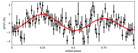
Low-mass white dwarfs in tight binaries can be tidally distorted by their more massive companions. Their projected sizes vary through their orbits, introducing signatures of ellipsoidal variations to time series photometric observations (e.g., Kilic et al. 2011; Vennes et al. 2011; Brown et al. 2011). Ellipsoidal variation signal periods are half the orbital periods, as demonstrated by the cartoon in Figure 1. Hermes et al. (2014) measured amplitudes of these signals from McDonald Observatory to better constrain the radii of low-mass white dwarf primaries in eight single-lined spectroscopic binaries. Bell et al. (2017) detected ellipsoidal variations in another double-degenerate binary, SDSS J1054$-$2121. This phase-folded light curve, averaged within 100 phase bins, is displayed in Figure 1. The best-fit model to the variations is overplotted. The effect of Doppler beaming, which causes the hot primary to appear brighter when approaching the observer, can also be seen (e.g., Zucker et al. 2007).

Figure 1: A cartoon depiction of ellipsoidal variations in a tight binary (not to scale) is displayed above the phase-folded and binned light curve of SDSS J1054$-$2121. The period of the ellipsoidal variation signal is half the orbital period.

2 Monte Carlo Rejection
Sampling

We refine the Monte Carlo approach of Hermes et al. (2014) to better constrain all parameters of low-mass white dwarf binaries that exhibit ellipsoidal variations. Here we demonstrate our rejection sampling method, giving specific values for the analysis of SDSS J1054$-$2121 (Figure 1; Bell et al. 2017).

For each star, we draw $10^{7}$ random deviates from Gaussians representing each of our observed quantities. Then we sample the probability density functions for the binary parameters of interest by calculating them from each set of deviates.

The ELM Survey (e.g., Brown et al. 2016) provides spectroscopic measurements and uncertainties for the effective temperatures ($T_{\mathrm{eff}}$), log surface gravities ($\log{g}$), orbital periods ($P$), and radial velocity semi-amplitudes ($K_{1}$) of all of our systems. We can already use these to constrain other physical properties of these binaries by assuming an isotropic prior on the inclination angle ($i$), as we demonstrate in Section 2.1. In Section 2.2, we include our measurements of the photometric ellipsoidal variation signal amplitudes to improve these constraints considerably.

The approach rests on a few simplifying assumptions: (1) that the rotation periods of the tidally deformed stars $\approx$ the binary periods; (2) that the light curves are records of significant flux from only the primary stars of the single-lined spectroscopic binaries; (3) that the mass of the secondaries are $<3$ $M_{\odot}$, corresponding to other white dwarfs or neutron stars; and (4) that there do not exist strong covariances between the measurements of these input quantities.

Figure 2: Marginal distributions of Monte Carlo samples for parameters of the binary system SDSS J1054$-$2121. The black histograms represent the original samples (some truncated), the dark gray histograms show samples that satisfy $M_{2}<3$ $M_{\odot}$ (based on spectroscopy only), and our final constraints that are informed by the measurement of the photometric ellipsoidal variation amplitude, $A_{\rm EV}$, are displayed in light gray. Definitions and summary statistics are in Table 1.

Table 1: System parameters for SDSS J1054$-$2121.

Parameter Name	Symbol	Units	Spectroscopy Only	With $A_{\rm EV}$
orbital period	$P$	days	$0.104\pm 0.007$	$0.096\begin{subarray}{c}+0.007\\ -0.006\end{subarray}$
RV semi-amplitude	$K_{1}$	km s-1	$261\pm 7$	$261\pm 7$
surface gravity	$\log(g)$	$g$ in cm s-2	$6.14\pm 0.11$	$5.75\pm 0.05$
effective temperature	$T_{\rm eff}$	K	$9220\pm 130$	$9010\begin{subarray}{c}+150\\ -130\end{subarray}$
ellipsoidal variation amp.	$A_{\rm EV}$	%	$0.13\begin{subarray}{c}+0.07\\ -0.05\end{subarray}$	$0.66\pm 0.08$
primary ELM mass	$M_{1}$	$M_{\odot}$	$0.166\pm 0.006$	$0.1546\begin{subarray}{c}+0.0016\\ -0.0015\end{subarray}$
primary ELM radius	$R_{1}$	$R_{\odot}$	$0.057\begin{subarray}{c}+0.007\\ -0.006\end{subarray}$	$0.087\pm 0.005$
orbital inclination	$i$	$\deg$	$63\begin{subarray}{c}+19\\ -23\end{subarray}$	$72\begin{subarray}{c}+9\\ -10\end{subarray}$
secondary mass	$M_{2}$	$M_{\odot}$	$0.49\begin{subarray}{c}+0.50\\ -0.09\end{subarray}$	$0.40\begin{subarray}{c}+0.06\\ -0.04\end{subarray}$
star-star separation	$a$	$R_{\odot}$	$0.82\begin{subarray}{c}+0.16\\ -0.07\end{subarray}$	$0.73\begin{subarray}{c}+0.05\\ -0.04\end{subarray}$
merger timescale	$\tau_{\rm merge}$	Gyr	$1.2\begin{subarray}{c}+0.3\\ -0.5\end{subarray}$	$1.2\pm 0.2$

2.1 Constraints from Spectroscopy

The spectroscopic parameters from the ELM Survey for SDSS J1054$-$2121 were provided in Gianninas et al. (2015): $T_{\rm eff}=9210\pm 140$ K; $\log{g}=6.14\pm 0.13$; $P_{\rm orb}=0.104\pm 0.007$ days; $K=261.1\pm 7.1$ km s^-1. The $\log{g}$ and $T_{\rm eff}$ have been corrected based on 3D convection simulations (Tremblay et al. 2015).

Without a measured photometric ellipsoidal variation amplitude, we can still progagate these measurements to constrain other properties of these binary systems with a Monte Carlo approach. We draw $10^{7}$ random deviates from Gaussians representing each of the observed spectroscopic quantities, as well as random inclination angles from a uniform $\cos{i}$ distribution. For each set of values, we sample the distributions of derived properties as follows:

• We interpolate the linear limb darkening coefficient, $u_{1}$, for each $\log{g}$ and $T_{\rm eff}$ from Gianninas et al. (2013). We use the values calculated for the LSST $g$ band as a proxy for BG40, which has a similar central wavelength.

• We calculate temperature-dependent gravity-darkening coefficients, $\tau_{1}$, following Morris (1985), using $\beta=0.25$ (the law of von Zeipel 1924) and 5000 Å as a representative central wavelength of the $BG40$ bandpass.

• Direct bilinear interpolation of Table 3 from Althaus et al. (2013) gives a mean and standard deviation spread of their evolutionary ELM model masses that could correspond to each $\log{g}$ and $T_{\rm eff}$ deviate pair. We select a random deviate for $M_{1}$ from the corresponding Gaussian distribution.

• The ELM white dwarf radius, $R_{1}$, follows directly from the definition $g=GM_{1}/R_{1}^{2}$.

• We calculate the secondary mass, $M_{2}$, from the measured mass function:

  $$P_{\rm orb}K^{3}_{1}/2\pi G=M^{3}_{2}\sin^{3}{i}/(M_{1}+M_{2})^{2}.$$

• We calculate the expected photometric semi-amplitude of ellipsoidal variations (in cgs units; Morris & Naftilan 1993 rearranged by Hermes et al. 2014):

  $$A_{\rm EV}=\frac{3\pi^{2}(15+u_{1})(1+\tau_{1})M_{2}R^{3}_{1}\sin^{2}{i}}{5P_{\rm orb}^{2}(3-u_{1})GM_{1}(M_{1}+M_{2})}.$$

• The orbital separation, $a$, comes from solving Kepler’s third law: $a^{3}=GP^{2}(M_{1}+M_{2})/4\pi^{2}$.

• Finally, we calculate the timescale to a binary merger caused by the release of orbital energy from gravitational radiation using the relation (for mass in $M_{\odot}$, period in hours; Landau & Lifshitz 1971)

  $$\tau_{\rm merge}=\frac{(M_{1}+M_{2})^{1/3}}{M_{1}M_{2}}P^{8/3}\times 10^{-2}{\rm\ Gyr.}$$

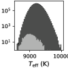
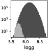
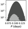
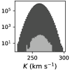
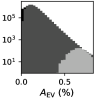
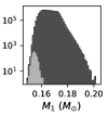
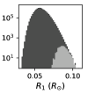
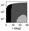
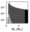
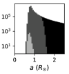
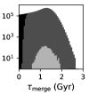
Physically, we expect a white dwarf or neutron star secondary with mass $M_{2}<3$ $M_{\odot}$. We reject solutions that violate this inequality, effectively accepting solutions in proportion to a step function prior on companion mass. The marginal distribution for each parameter from the initial random deviates is displayed in black in Figure 2. The samples that survive the rejection step based on secondary mass are shown in dark gray. We summarize our constraints on these parameters in the “Spectroscopy Only” column of Table 1 by listing the median values, with uncertainties giving the distances to the 15.9 and 84.1 percentiles. While this percentile range contains the middle 68.2% of the samples, many of these distributions are decidedly non-Gaussian, as can be seen in Figure 2.

This Monte Carlo approach allows us to propagate our measurements and priors through combinations of model grids and analytic functions to understand the parameter space of unobserved quantities. An immediately obvious application of this is to identify ELM binary systems that are likely to exhibit ellipsoidal variations for photometric follow-up.

2.2 Constraints with Ellipsoidal
Variations

For systems with measured ellipsoidal variation amplitudes, $A_{\mathrm{EV}}$, we can further reduce the solution space to include only those parameter combinations that provide agreement between the observations and the model. For SDSS J1054$-$2121, $A_{\mathrm{EV}}=0.75\pm 0.08$% (Bell et al. 2017). We incorporate Gaussian samples for $A_{\mathrm{EV}}$ into our Monte Carlo framework and numerically solve for $i$ and $M_{2}$. We still require $M_{2}<3M_{\mathrm{\odot}}$. For $10^{7}$ Monte Carlo samples, we accept solutions in proportion to an isotropic prior on inclination (rejecting nonphysical $\sin{i}>1$).

The light gray histograms in Figure 2 demonstrate our improved constraints on the parameters of SDSS J1054$-$2121. The $A_{\mathrm{EV}}$ measurement most significantly restricts the viable range for orbital inclination. However, we note that only 0.013% of our samples are not rejected for this particular system, implying that our model and measurements are not in very close agreement. Our final constraints are included in the “With $A_{\mathrm{EV}}$” column of Table 1. Our results support that the unseen companion in SDSS J1054$-$2121 is likely another white dwarf.

3 Ensemble Radius–Mass
Constraints

Figure 3: Radius and mass constraints from Monte Carlo sampling.

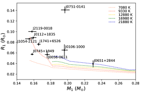
Following the method in Section 2.2, we constrain the parameters of nine low-mass white dwarf binaries that show ellipsoidal variations (Hermes et al. 2014; Bell et al. 2017). We plot the mass and radius constraints in Figure 3 (mimicking Figure 5 of Hermes et al. 2014). We also display the radius–mass relations at different temperatures from the evolutionary cooling tracks of Althaus et al. (2013). Because these models are used in our Monte Carlo calculations, our measurements follow these tracks by design. The observations for SDSS J0751$-$0141 best fit a pre-white-dwarf model that is still contracting toward a cooling track.

Our new constraints on $R_{1}$ and $i$ are compared to the values from Hermes et al. (2014) in Table 2. These agree overall, as they should since they are based on the same measurements. Our new quoted uncertainties are smaller due to a different rejection scheme. The only discrepancy is for SDSS J0745+1949, for which only 0.0074% of our samples (all at the $M_{2}\approx 3M_{\odot}$ limit) survive rejection, indicating considerable disagreement between the measurements and the model.

4 Comparison with Gaia Radii

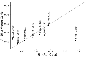
With the recent availability of Gaia astrometry, we can place independent constraints on stellar radii based on astrometric distance. Eight of our stars have positive parallax measurements in Gaia DR2. We make quick approximations of the distances to these stars by simply inverting Monte Carlo samples within the Gaussian uncertainties of the parallax measurements. We then scale the stellar radii at these distances from representative DA (hydrogen-atmosphere) white dwarf model magnitudes (Holberg & Bergeron 2006; Kowalski & Saumon 2006; Tremblay et al. 2011) until they match the observed magnitudes (similar to the solid angle approach of Pelisoli et al. 2018). We compare the results of our Monte Carlo analysis to the constraints from Gaia in Figure 4. The systems that show significant disagreement between these independent radius determinations are useful for tracing systematic errors in our measurements, models, or their interpretation.

Figure 4: Comparison of independent radius constraints from Monte Carlo sampling and from Gaia astrometry.

5 Summary and Prospects

We have demonstrated a work-in-progress Monte Carlo rejection sampling approach for improving constraints on low-mass white dwarf binary systems that exhibit ellipsoidal variations. Ellipsoidal variation amplitudes are particularly helpful for constraining the orbital inclination, and thereby the secondary mass and orbital separation. However, the miniscule fractions of values that survive rejection sampling for some stars indicate a lack of agreement between the measurements and the model. These discrepancies provide a tool for identifying systematic errors in our analysis. The concentration of our final distribution for $\log{g}$ in the far wing of the prior distribution for SDSS J1054$-$2121 in Figure 2 suggests that surface gravity may particularly suffer systematic errors (also suggested in this regime by Brown et al. 2017). This is corroborated by disagreements with the independent radius constraints from Gaia astrometry. Incorporating the Gaia radii into this framework could improve our surface gravity determinations for tidally distorted white dwarfs and inform our future interpretation of white dwarf spectra.

Table 2: Parameters constrained by ellipsoidal variations for the Hermes et al. (2014) sample.

	Hermes et al. 2014		This Work
SDSS	$R_{1}$ ($R_{\odot}$)	$i$ ($\deg$)	$R_{1}$ ($R_{\odot}$)	$i$ ($\deg$)
J0056$-$0611	$0.056\pm 0.006$	$50\begin{subarray}{c}+22\\ -13\end{subarray}$	$0.057\pm 0.002$	$50\begin{subarray}{c}+9\\ -7\end{subarray}$
J0106$-$1000	$0.063\pm 0.008$	$60\begin{subarray}{c}+29\\ -20\end{subarray}$	$0.065\begin{subarray}{c}+0.004\\ -0.003\end{subarray}$	$56\begin{subarray}{c}+11\\ -8\end{subarray}$
J0112+1835	$0.088\pm 0.009$	$70\begin{subarray}{c}+20\\ -19\end{subarray}$	$0.089\begin{subarray}{c}+0.004\\ -0.003\end{subarray}$	$66\begin{subarray}{c}+10\\ -9\end{subarray}$
J0651+2844	$0.040\pm 0.002$	$83\begin{subarray}{c}+7\\ -8\end{subarray}$	$0.0393\begin{subarray}{c}+0.0007\\ -0.0006\end{subarray}$	$79\begin{subarray}{c}+5\\ -7\end{subarray}$
J0745+1949	$0.176\begin{subarray}{c}+0.090\\ -0.025\end{subarray}$	$63\begin{subarray}{c}+27\\ -32\end{subarray}$	$0.0572\pm 0.0017$	$10.5\pm 0.4$
J0751$-$0141	$0.138\begin{subarray}{c}+0.012\\ -0.007\end{subarray}$	$77\begin{subarray}{c}+13\\ -17\end{subarray}$	$0.141\begin{subarray}{c}+0.006\\ -0.005\end{subarray}$	$72\pm 9$
J1741+6526	$0.076\pm 0.006$	$78\begin{subarray}{c}+12\\ -16\end{subarray}$	$0.0762\begin{subarray}{c}+0.0023\\ -0.0019\end{subarray}$	$75\begin{subarray}{c}+7\\ -8\end{subarray}$
J2119$-$0018	$0.103\pm 0.016$	$75\begin{subarray}{c}+15\\ -21\end{subarray}$	$0.100\begin{subarray}{c}+0.005\\ -0.004\end{subarray}$	$68\begin{subarray}{c}+10\\ -11\end{subarray}$

Acknowledgements. We gratefully acknowledge support from NSF grant AST-1312983 that funded our data acquisition at McDonald Observatory. Participation in the 21^st European Workshop on White Dwarfs was funded by the European Research Council under the European Community’s Seventh Framework Programme (FP7/2007-2013) / ERC grant agreement no 338251 (Stellar Ages). An early version of this work was included in K.J.B.’s PhD Thesis (U. Texas). We thank Warren Brown and Mukremin Kilic for comments on the poster, and E. L. Robinson for discussions about the method.

References

- Althaus et al. (2013) Althaus, L. G., Miller Bertolami, M. M., & Córsico, A. H. 2013, A&A, 557, A19
- Bell et al. (2017) Bell, K. J., Gianninas, A., Hermes, J. J., et al. 2017, ApJ, 835, 180
- Brown et al. (2016) Brown, W. R., Gianninas, A., Kilic, M., Kenyon, S. J., & Allende Prieto, C. 2016, ApJ, 818, 155
- Brown et al. (2010) Brown, W. R., Kilic, M., Allende Prieto, C., & Kenyon, S. J. 2010, ApJ, 723, 1072
- Brown et al. (2017) Brown, W. R., Kilic, M., & Gianninas, A. 2017, ApJ, 839, 23
- Brown et al. (2011) Brown, W. R., Kilic, M., Hermes, J. J., et al. 2011, ApJ, 737, L23
- Gianninas et al. (2015) Gianninas, A., Kilic, M., Brown, W. R., Canton, P., & Kenyon, S. J. 2015, ApJ, 812, 167
- Gianninas et al. (2013) Gianninas, A., Strickland, B. D., Kilic, M., & Bergeron, P. 2013, ApJ, 766, 3
- Hermes et al. (2014) Hermes, J. J., Brown, W. R., Kilic, M., et al. 2014, ApJ, 792, 39
- Holberg & Bergeron (2006) Holberg, J. B., & Bergeron, P. 2006, AJ, 132, 1221
- Kilic et al. (2011) Kilic, M., Brown, W. R., Kenyon, S. J., et al. 2011, MNRAS, 413, L101
- Kilic et al. (2007) Kilic, M., Stanek, K. Z., & Pinsonneault, M. H. 2007, ApJ, 671, 761
- Kowalski & Saumon (2006) Kowalski, P. M., & Saumon, D. 2006, ApJ, 651, L137
- Landau & Lifshitz (1971) Landau, L. D., & Lifshitz, E. M. 1958, The Classical Theory of Fields, (Oxford: Oxford Pergamon Press)
- Morris (1985) Morris, S. L. 1985, ApJ, 295, 143
- Morris & Naftilan (1993) Morris, S. L., & Naftilan, S. A. 1993, ApJ, 419, 344
- Nelemans et al. (2001) Nelemans, G., Yungelson, L. R., Portegies Zwart, S. F., & Verbunt, F. 2001, A&A, 365, 491
- Pelisoli et al. (2018) Pelisoli, I., Bell, K. J., Kepler, S. O., & Koester, D. 2018, arXiv:1805.04070
- Tremblay et al. (2011) Tremblay, P.-E., Bergeron, P., & Gianninas, A. 2011, ApJ, 730, 128
- Tremblay et al. (2015) Tremblay, P.-E., Gianninas, A., Kilic, M., et al. 2015, ApJ, 809, 148
- Vennes et al. (2011) Vennes, S., Thorstensen, J. R., Kawka, A., et al. 2011, ApJ, 737, L16
- von Zeipel (1924) von Zeipel, H. 1924, MNRAS, 84, 665
- Zucker et al. (2007) Zucker, S., Mazeh, T., & Alexander, T. 2007, ApJ, 670, 1326