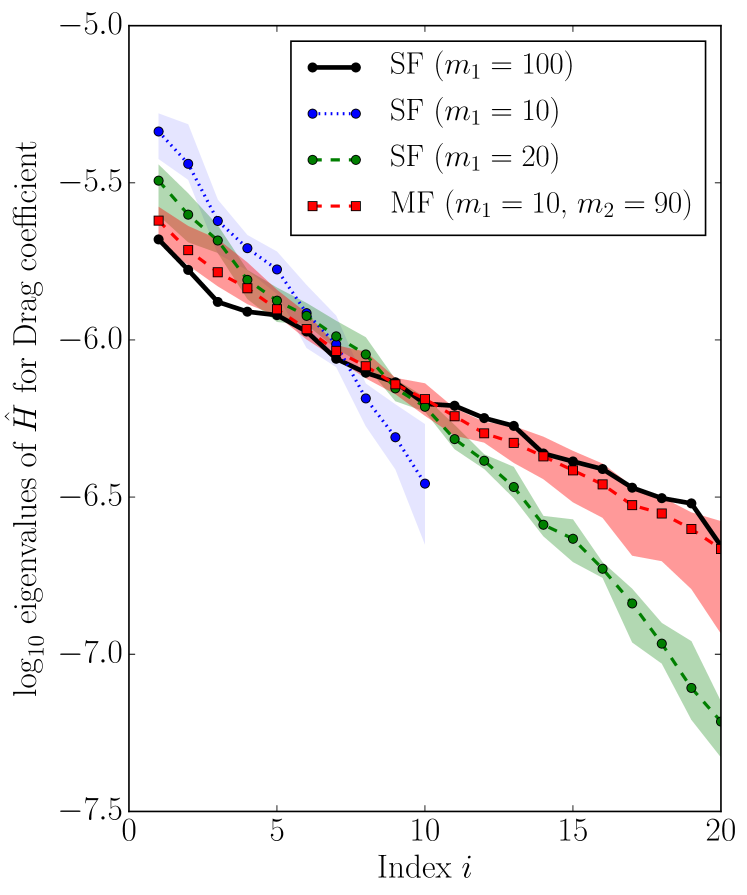
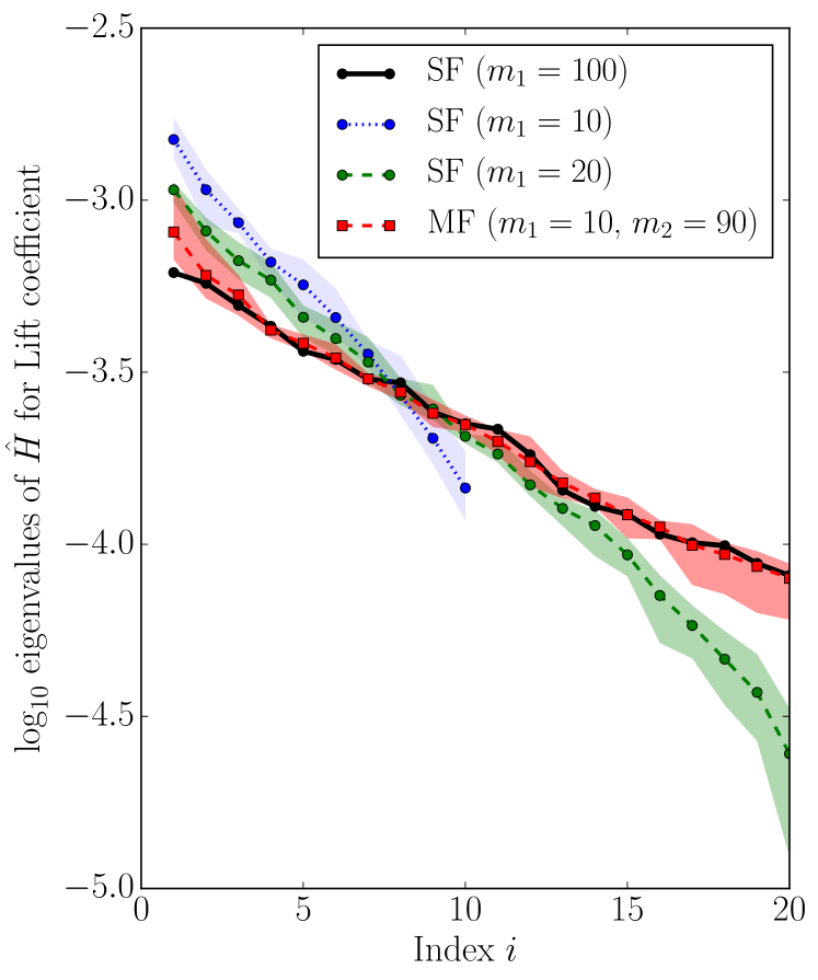
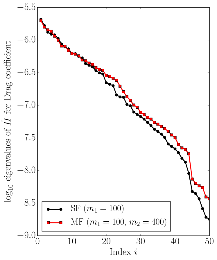
\newsiamremark

remarkRemark \newsiamremarkhypothesisHypothesis \newsiamthmclaimClaim \headersMultifidelity Dimension Reduction via Active SubspacesR. Lam, O. Zahm, Y. Marzouk, and K. Willcox

Multifidelity Dimension Reduction
via Active Subspacesthanks: Submitted to the editors on 09/14/2018. \fundingThis work was funded in part by the AFOSR MURI on multi-information sources of multi-physics systems under Award Number FA9550-15-1-0038, program manager Dr. Fariba Fahroo.

Remi R. Lam Department of Aeronautics and Astronautics, Massachusetts Institute of Technology, Cambridge, MA 02139 (, ). rlam@mit.edu ymarz@mit.edu    Olivier Zahm Université Grenoble Alpes, Inria, CNRS, Grenoble INP, LJK, 38000 Grenoble, France (). olivier.zahm@inria.fr    Youssef M. Marzouk22footnotemark: 2    Karen E. Willcox Oden Institute for Computational Engineering and Sciences, UT Austin, Austin, TX 78712 () kwillcox@oden.utexas.edu
Abstract

We propose a multifidelity dimension reduction method to identify a low-dimensional structure present in many engineering models. The structure of interest arises when functions vary primarily on a low-dimensional subspace of the high-dimensional input space, while varying little along the complementary directions. Our approach builds on the gradient-based methodology of active subspaces, and exploits models of different fidelities to reduce the cost of performing dimension reduction through the computation of the active subspace matrix. We provide a non-asymptotic analysis of the number of gradient evaluations sufficient to achieve a prescribed error in the active subspace matrix, both in expectation and with high probability. We show that the sample complexity depends on a notion of intrinsic dimension of the problem, which can be much smaller than the dimension of the input space. We illustrate the benefits of such a multifidelity dimension reduction approach using numerical experiments with input spaces of up to two thousand dimensions.

keywords:
Dimension reduction, multifidelity, gradient-based, active subspace, intrinsic dimension, effective rank, matrix Bernstein inequality, control variate.
{AMS}

15A18, 15A60, 41A30, 41A63, 65D15, 65N30

1 Introduction

Engineering models are typically parameterized by a large number of input variables, and can also be expensive to evaluate. Yet these models are often embedded in problems of global optimization or uncertainty quantification, whose computational cost and complexity increase dramatically with the number of model inputs. One strategy to circumvent this curse of dimensionality is to exploit, when present, some notion of low-dimensional structure and to perform dimension reduction. Doing so can significantly reduce the complexity of the problem at hand. In this paper, we consider the problem of identifying the low-dimensional structure that arises when an output of a model varies primarily on a low-dimensional subspace of the input space, while varying little along the complementary directions. This structure is commonly found in engineering problems and can be identified using the active subspace method [39, 7], among other methods. The active subspace method relies on the computation of a second moment matrix, a step that can be costly as it often involves many evaluations of the gradient of the model. In this work, we consider the common engineering setting where cheap low-fidelity approximations of an expensive high-fidelity model, and its gradients, are available. We propose a multifidelity gradient-based algorithm to reduce the cost of performing dimension reduction via active subspaces. In particular, we present a multifidelity estimator of the second moment matrix used by the active subspace method and show, theoretically and empirically, that fewer evaluations of the expensive gradient are sufficient to perform dimension reduction.

Several approaches have been devised to identify low-dimensional structure in the input space of a function. These methods include global sensitivity analysis [41], sliced inverse regression [27], basis adaptation [46], and low-rank matrix recovery [48]. Recent work has also explored combining dimension reduction in both the input and the state space of the associated model [28, 16, 40, 12, 45, 2]. Such methods typically require a large number of (potentially expensive) function evaluations. When derivative information is available (e.g., via adjoint methods or automatic differentiation), gradient-based methods have also been proposed to detect the low-dimensional structure of a smooth function, with higher sample efficiency [42]. One way to leverage derivative information is to examine the spectral properties of the second moment matrix of the gradient of the function. The dominant eigenspace of that matrix contains the directions along which the function, loosely speaking, varies the most. This dominant eigenspace is called the active subspace [39, 9, 7]. More precisely, in [50], the second moment matrix is used to construct an upper bound for the function approximation error induced by dimension reduction. The active subspace’s dimension is then chosen in order to satisfy a user-defined tolerance, allowing a rigorous control of the approximation error. Gradient-based methods have been successfully used to detect and exploit low-dimensional structure in engineering models [29, 18, 8, 19] as well as in Bayesian inverse problems [11, 10, 51]. The efficiency of these gradient-based methods depends upon the computation of the second moment matrix of the gradient. This can be an expensive step as it involves computing an integral, over the high-dimensional input space, of the gradient of an expensive function. Reducing the cost of the dimension reduction step is particularly important as it allows more computational resources to be allocated to the original task of interest (e.g., optimization or uncertainty quantification).

To reduce this computational cost, one strategy consists of replacing the expensive gradient with a cheap-to-evaluate approximation or surrogate. Surrogates with lower evaluation cost are widely available in engineering problems: they include models defined by numerically solving equations on coarser meshes, using simplified governing equations, imposing looser convergence criteria, or employing reduced-order models. In order to control the error induced by the use of a surrogate, multifidelity methods aim at combining cheap approximations with expensive but accurate information in an optimal way (see [35] for a survey). The goal of such approaches is to shift most of the work to the cheaper model, while querying the expensive model often enough to guarantee convergence to the desired quantity (in this case, the second moment matrix of the gradient). For instance, multigrid methods use a hierarchy of cheaper and coarser discretizations to solve systems of partial differential equations more efficiently [4, 5, 15]. In multilevel Monte Carlo, expected quantities and rare event probabilities are computed by distributing the computational work among several levels of approximation with known error rate and cost [14, 44, 49, 22, 3]. When no such information about error rates is available, or when there is no hierarchy among models, multifidelity techniques have been employed to accelerate Monte Carlo estimates [36] by solving an optimal resource allocation problem among a collection of models with varying fidelity. Multifidelity techniques have also been devised to accelerate optimization [1, 13, 30, 43, 24, 37, 20], global sensitivity analysis [38], or importance sampling and rare event estimation [26, 25, 34, 33]. While most multifidelity techniques have focused on estimating the expectations of scalar quantities, high-dimensional objects such as the second moment matrix in the active subspace method—effectively, the expectation of a matrix-valued function—have received less attention. Because high-dimensional objects are typically more challenging to approximate, developing and analyzing multifidelity algorithms for their estimation could lead to significant computational savings.

In this paper, we use multifidelity techniques to reduce the computational cost of performing dimension reduction. We build on the gradient-based active subspace method, proposing a multifidelity estimator for the second moment matrix that uses the low-fidelity model as a control variate for the outputs of the high-fidelity model—thus providing variance reduction and reducing computational costs. We establish non-asymptotic error bounds for this estimator, both in expectation and in high probability. We show that the sample complexity depends on the intrinsic dimension of the second moment matrix, a quantity that can be much smaller than the dimension of the input space when the function of interest varies mostly along a few directions. Finally, we demonstrate the performance of our proposed multifidelity dimension reduction technique on several analytical and engineering examples.

The paper is organized as follows. In Section 2, we give a brief review of the active subspace methodology. Then, we formalize the proposed active subspace multifidelity algorithm in Section 3. Error bounds for the single-fidelity and multifidelity active subspace algorithms are provided in Section 4. We illustrate the benefits of our approach with numerical examples in Section 5 before summarizing our findings in Section 6.

2 Active subspace

We consider a scalar-valued function f:𝒳:𝑓𝒳{\color[rgb]{0,0,0}\definecolor[named]{pgfstrokecolor}{rgb}{0,0,0}\pgfsys@color@gray@stroke{0}\pgfsys@color@gray@fill{0}f}:\mathcal{X}\to\mathbb{R} where the input space 𝒳𝒳\mathcal{X} is a subset of dsuperscript𝑑\mathbb{R}^{{\color[rgb]{0,0,0}\definecolor[named]{pgfstrokecolor}{rgb}{0,0,0}\pgfsys@color@gray@stroke{0}\pgfsys@color@gray@fill{0}d}}. We refer to the dimension d𝑑{\color[rgb]{0,0,0}\definecolor[named]{pgfstrokecolor}{rgb}{0,0,0}\pgfsys@color@gray@stroke{0}\pgfsys@color@gray@fill{0}d}\in\mathbb{N} as the ambient dimension. The active subspace method [9, 7] aims to compute a low-dimensional subspace of 𝒳𝒳\mathcal{X} in which most of the variations of f𝑓{\color[rgb]{0,0,0}\definecolor[named]{pgfstrokecolor}{rgb}{0,0,0}\pgfsys@color@gray@stroke{0}\pgfsys@color@gray@fill{0}f} are concentrated. The active subspace method assumes that f𝑓{\color[rgb]{0,0,0}\definecolor[named]{pgfstrokecolor}{rgb}{0,0,0}\pgfsys@color@gray@stroke{0}\pgfsys@color@gray@fill{0}f} is differentiable and that each component of f𝑓\nabla f is square integrable on the space 𝒳𝒳\mathcal{X}, weighted by a user-defined probability density ρ:𝒳+:𝜌𝒳superscript\rho:\mathcal{X}\to\mathbb{R}^{+}. This guarantees the well posedness of the second moment matrix

H=𝔼[f(X)f(X)T],𝐻𝔼delimited-[]𝑓𝑋𝑓superscript𝑋𝑇\displaystyle H={\color[rgb]{0,0,0}\definecolor[named]{pgfstrokecolor}{rgb}{0,0,0}\pgfsys@color@gray@stroke{0}\pgfsys@color@gray@fill{0}\mathbb{E}}\left[\nabla f(X)\nabla f(X)^{T}\right],

where Xρsimilar-to𝑋𝜌X\sim\rho is a random variable taking values in 𝒳𝒳\mathcal{X} and 𝔼[]𝔼delimited-[]{\color[rgb]{0,0,0}\definecolor[named]{pgfstrokecolor}{rgb}{0,0,0}\pgfsys@color@gray@stroke{0}\pgfsys@color@gray@fill{0}\mathbb{E}}[\,\cdot\,] denotes the expectation. We refer to H𝐻H as the active subspace matrix (AS matrix). The eigendecomposition of H𝐻H yields information about the directions along which f𝑓{\color[rgb]{0,0,0}\definecolor[named]{pgfstrokecolor}{rgb}{0,0,0}\pgfsys@color@gray@stroke{0}\pgfsys@color@gray@fill{0}f} varies. Specifically, for any unit norm vector ud𝑢superscript𝑑u\in\mathbb{R}^{{\color[rgb]{0,0,0}\definecolor[named]{pgfstrokecolor}{rgb}{0,0,0}\pgfsys@color@gray@stroke{0}\pgfsys@color@gray@fill{0}d}}, the quantity uTHu=𝔼[(f(X)Tu)2]superscript𝑢𝑇𝐻𝑢𝔼delimited-[]superscript𝑓superscript𝑋𝑇𝑢2u^{T}Hu={\color[rgb]{0,0,0}\definecolor[named]{pgfstrokecolor}{rgb}{0,0,0}\pgfsys@color@gray@stroke{0}\pgfsys@color@gray@fill{0}\mathbb{E}}[(\nabla f(X)^{T}u)^{2}] corresponds to the L2superscript𝐿2L^{2} norm of the gradient f𝑓\nabla f projected on span{u}span𝑢\text{span}\{u\}. Thus, the largest eigenvector of H𝐻H, which is a maximizer of uTHusuperscript𝑢𝑇𝐻𝑢u^{T}Hu over unit norm vectors ud𝑢superscript𝑑u\in\mathbb{R}^{{\color[rgb]{0,0,0}\definecolor[named]{pgfstrokecolor}{rgb}{0,0,0}\pgfsys@color@gray@stroke{0}\pgfsys@color@gray@fill{0}d}}, is aligned with the direction in which f𝑓{\color[rgb]{0,0,0}\definecolor[named]{pgfstrokecolor}{rgb}{0,0,0}\pgfsys@color@gray@stroke{0}\pgfsys@color@gray@fill{0}f} has largest (in squared magnitude) average derivative.

Another important property is that, under some mild assumptions on the probability density ρ𝜌\rho, the AS matrix allows us to control the mean square error between f(X)𝑓𝑋{\color[rgb]{0,0,0}\definecolor[named]{pgfstrokecolor}{rgb}{0,0,0}\pgfsys@color@gray@stroke{0}\pgfsys@color@gray@fill{0}f}(X) and a ridge approximation of the form of h(UrTX)superscriptsubscript𝑈𝑟𝑇𝑋h(U_{r}^{T}X), where Urd×rsubscript𝑈𝑟superscript𝑑𝑟U_{r}\in\mathbb{R}^{{\color[rgb]{0,0,0}\definecolor[named]{pgfstrokecolor}{rgb}{0,0,0}\pgfsys@color@gray@stroke{0}\pgfsys@color@gray@fill{0}d}\times r} is a matrix with rd𝑟𝑑r\leq{\color[rgb]{0,0,0}\definecolor[named]{pgfstrokecolor}{rgb}{0,0,0}\pgfsys@color@gray@stroke{0}\pgfsys@color@gray@fill{0}d} orthonormal columns. In particular, if hh is defined to be the conditional expectation h(UrTX)=𝔼[f(X)|UrTX]superscriptsubscript𝑈𝑟𝑇𝑋𝔼delimited-[]conditional𝑓𝑋superscriptsubscript𝑈𝑟𝑇𝑋h(U_{r}^{T}X)={\color[rgb]{0,0,0}\definecolor[named]{pgfstrokecolor}{rgb}{0,0,0}\pgfsys@color@gray@stroke{0}\pgfsys@color@gray@fill{0}\mathbb{E}}[f(X)|U_{r}^{T}X], 𝒳=d𝒳superscript𝑑\mathcal{X}=\mathbb{R}^{{\color[rgb]{0,0,0}\definecolor[named]{pgfstrokecolor}{rgb}{0,0,0}\pgfsys@color@gray@stroke{0}\pgfsys@color@gray@fill{0}d}}, and ρ𝜌\rho is the density of the standard normal distribution on 𝒳𝒳\mathcal{X}, then Proposition 2.5 in [50] (with Pr=UrUrTsubscript𝑃𝑟subscript𝑈𝑟superscriptsubscript𝑈𝑟𝑇P_{r}=U_{r}U_{r}^{T}) guarantees that

(1) 𝔼[(f(X)h(UrTX))2]trace(H)trace(UrTHUr),𝔼delimited-[]superscript𝑓𝑋superscriptsubscript𝑈𝑟𝑇𝑋2trace𝐻tracesuperscriptsubscript𝑈𝑟𝑇𝐻subscript𝑈𝑟{\color[rgb]{0,0,0}\definecolor[named]{pgfstrokecolor}{rgb}{0,0,0}\pgfsys@color@gray@stroke{0}\pgfsys@color@gray@fill{0}\mathbb{E}}[({\color[rgb]{0,0,0}\definecolor[named]{pgfstrokecolor}{rgb}{0,0,0}\pgfsys@color@gray@stroke{0}\pgfsys@color@gray@fill{0}f}(X)-h(U_{r}^{T}X))^{2}]\leq\operatorname{trace}(H)-\operatorname{trace}(U_{r}^{T}HU_{r}),

holds for any Ursubscript𝑈𝑟U_{r} such that UrTUr=Irsuperscriptsubscript𝑈𝑟𝑇subscript𝑈𝑟subscript𝐼𝑟U_{r}^{T}U_{r}=I_{r}. This result relies on Poincaré-type inequalities and can be extended to more general densities ρ𝜌\rho (see Corollary 2 in [51]). In order to obtain a good approximation of f𝑓{\color[rgb]{0,0,0}\definecolor[named]{pgfstrokecolor}{rgb}{0,0,0}\pgfsys@color@gray@stroke{0}\pgfsys@color@gray@fill{0}f} in the L2superscript𝐿2L^{2} sense, we can choose Ursubscript𝑈𝑟U_{r} as a matrix which minimizes the right-hand side of (1). This is equivalent to the problem

(2) maxUrd×rs.t. UrTUr=Irtrace(UrTHUr).subscriptsubscript𝑈𝑟superscript𝑑𝑟s.t. superscriptsubscript𝑈𝑟𝑇subscript𝑈𝑟subscript𝐼𝑟tracesuperscriptsubscript𝑈𝑟𝑇𝐻subscript𝑈𝑟\max_{\begin{subarray}{c}U_{r}\in\mathbb{R}^{{\color[rgb]{0,0,0}\definecolor[named]{pgfstrokecolor}{rgb}{0,0,0}\pgfsys@color@gray@stroke{0}\pgfsys@color@gray@fill{0}d}\times r}\\ \text{s.t. }U_{r}^{T}U_{r}=I_{r}\end{subarray}}\operatorname{trace}(U_{r}^{T}HU_{r}).

Any matrix Ursubscript𝑈𝑟U_{r} whose columns span the r𝑟r-dimensional dominant eigenspace of H𝐻H is a solution. The corresponding subspace is called the active subspace.

In practice, there is no closed-form expression for the AS matrix and H𝐻H must be approximated numerically. The following Monte Carlo estimator requires evaluating f𝑓\nabla f at m1subscript𝑚1m_{1} realizations of the input parameters, drawn independently from ρ𝜌\rho. We refer to this estimator as a single-fidelity estimator (SF estimator).

Definition 2.1 (Single-fidelity estimator).

Let m11subscript𝑚11m_{1}\geq 1 be the number of gradient evaluations. We define the SF estimator of H𝐻H to be

H^SF=subscript^𝐻𝑆𝐹absent\displaystyle\widehat{H}_{SF}= 1m1i=1m1f(Xi)f(Xi)T,1subscript𝑚1superscriptsubscript𝑖1subscript𝑚1𝑓subscript𝑋𝑖𝑓superscriptsubscript𝑋𝑖𝑇\displaystyle\frac{1}{m_{1}}\sum_{i=1}^{m_{1}}\nabla f(X_{i})\nabla f(X_{i})^{T},

where X1,,Xm1subscript𝑋1subscript𝑋subscript𝑚1X_{1},\ldots,X_{m_{1}} are independent copies of Xρsimilar-to𝑋𝜌X\sim\rho.

Computing an estimate of H𝐻H with a satisfactory error can require a large number m1subscript𝑚1m_{1} of gradient evaluations. In the following section, we propose a new multifidelity algorithm that leverages a cheap-to-evaluate approximation of f𝑓\nabla f to reduce the cost of estimating H𝐻H.

3 Multifidelity dimension reduction

In this section, we describe a multifidelity approach for estimating the AS matrix H𝐻H (Sec. 3.1). We also characterize the impact of using such an approximation of H𝐻H on the quality of the dimension reduction (Sec. 3.2).

3.1 Multifidelity active subspace estimator

Suppose we are given a function g:𝒳:𝑔𝒳g:\mathcal{X}\to\mathbb{R} that is a cheap-to-evaluate approximation of f𝑓{\color[rgb]{0,0,0}\definecolor[named]{pgfstrokecolor}{rgb}{0,0,0}\pgfsys@color@gray@stroke{0}\pgfsys@color@gray@fill{0}f}. We assume that g𝑔g is differentiable and that each component of g𝑔\nabla g is square integrable. From now on, we refer to f𝑓{\color[rgb]{0,0,0}\definecolor[named]{pgfstrokecolor}{rgb}{0,0,0}\pgfsys@color@gray@stroke{0}\pgfsys@color@gray@fill{0}f} as the high-fidelity function and to g𝑔g as the low-fidelity function. Based on the identity

H=𝔼[f(X)f(X)Tg(X)g(X)T]+𝔼[g(X)g(X)T],𝐻𝔼delimited-[]𝑓𝑋𝑓superscript𝑋𝑇𝑔𝑋𝑔superscript𝑋𝑇𝔼delimited-[]𝑔𝑋𝑔superscript𝑋𝑇H={\color[rgb]{0,0,0}\definecolor[named]{pgfstrokecolor}{rgb}{0,0,0}\pgfsys@color@gray@stroke{0}\pgfsys@color@gray@fill{0}\mathbb{E}}[\nabla f(X)\nabla f(X)^{T}-\nabla g(X)\nabla g(X)^{T}]+{\color[rgb]{0,0,0}\definecolor[named]{pgfstrokecolor}{rgb}{0,0,0}\pgfsys@color@gray@stroke{0}\pgfsys@color@gray@fill{0}\mathbb{E}}[\nabla g(X)\nabla g(X)^{T}],

we introduce the following unbiased multifidelity estimator (MF estimator).

Definition 3.1 (Multifidelity estimator).

Let m11subscript𝑚11m_{1}\geq 1 and m21subscript𝑚21m_{2}\geq 1 be the numbers of gradient evaluations of f𝑓{\color[rgb]{0,0,0}\definecolor[named]{pgfstrokecolor}{rgb}{0,0,0}\pgfsys@color@gray@stroke{0}\pgfsys@color@gray@fill{0}f} and g𝑔g. We define the MF estimator of H𝐻H to be:

H^MFsubscript^𝐻𝑀𝐹\displaystyle\widehat{H}_{MF} =1m1i=1m1(f(Xi)f(Xi)Tg(Xi)g(Xi)T)+1m2i=m1+1m1+m2g(Xi)g(Xi)T,absent1subscript𝑚1superscriptsubscript𝑖1subscript𝑚1𝑓subscript𝑋𝑖𝑓superscriptsubscript𝑋𝑖𝑇𝑔subscript𝑋𝑖𝑔superscriptsubscript𝑋𝑖𝑇1subscript𝑚2superscriptsubscript𝑖subscript𝑚11subscript𝑚1subscript𝑚2𝑔subscript𝑋𝑖𝑔superscriptsubscript𝑋𝑖𝑇\displaystyle=\frac{1}{m_{1}}\sum_{i=1}^{m_{1}}(\nabla f(X_{i})\nabla f(X_{i})^{T}-\nabla g(X_{i})\nabla g(X_{i})^{T})+\frac{1}{m_{2}}\sum_{i=m_{1}+1}^{m_{1}+m_{2}}\nabla g(X_{i})\nabla g(X_{i})^{T},

where X1,,Xm1+m2subscript𝑋1subscript𝑋subscript𝑚1subscript𝑚2X_{1},\ldots,X_{m_{1}+m_{2}} are independent copies of Xρsimilar-to𝑋𝜌X\sim\rho.

Remark 3.2 (Indefiniteness of H^MFsubscript^𝐻𝑀𝐹\widehat{H}_{MF}).

While the quantity of interest H𝐻H is symmetric positive semi-definite, the multifidelity estimator H^MFsubscript^𝐻𝑀𝐹\widehat{H}_{MF} is symmetric but not necessarily positive semi-definite. It is natural to ask whether a positive semi-definite estimator is necessary to yield good dimension reduction. In the following, we show that the quality of the dimension reduction is controlled by the error between H𝐻H and H^MFsubscript^𝐻𝑀𝐹\widehat{H}_{MF} (Corollary 3.5) which can be reduced arbitrarily close to zero with high probability (Proposition 4.1). In particular, those results do not require positive semi-definiteness from the estimator H^MFsubscript^𝐻𝑀𝐹\widehat{H}_{MF}.

A realization of H^MFsubscript^𝐻𝑀𝐹\widehat{H}_{MF} can be obtained using Algorithm 1. First, m1+m2subscript𝑚1subscript𝑚2m_{1}+m_{2} input parameter realizations are drawn independently from ρ𝜌\rho. Then, the high-fidelity gradients are evaluated at the first m1subscript𝑚1m_{1} input parameter values while the low-fidelity gradients are evaluated at all m1+m2subscript𝑚1subscript𝑚2m_{1}+m_{2} input parameter values.

Algorithm 1 Multifidelity Active Subspace
  Function: multifidelity_active_subspace(m1,m2)subscript𝑚1subscript𝑚2(m_{1},m_{2})
  Input: m1subscript𝑚1m_{1} and m2subscript𝑚2m_{2}
  Draw m1+m2subscript𝑚1subscript𝑚2m_{1}+m_{2} independent copies {Xi}i=1m1+m2superscriptsubscriptsubscript𝑋𝑖𝑖1subscript𝑚1subscript𝑚2\{X_{i}\}_{i=1}^{m_{1}+m_{2}} of Xρsimilar-to𝑋𝜌X\sim\rho
  for i=1𝑖1i=1 to m1subscript𝑚1m_{1} do
     Compute f(Xi)𝑓subscript𝑋𝑖\nabla f(X_{i}) and g(Xi)𝑔subscript𝑋𝑖\nabla g(X_{i})
  end for
  H^MF1m1i=1m1(f(Xi)f(Xi)Tg(Xi)g(Xi)T)subscript^𝐻𝑀𝐹1subscript𝑚1superscriptsubscript𝑖1subscript𝑚1𝑓subscript𝑋𝑖𝑓superscriptsubscript𝑋𝑖𝑇𝑔subscript𝑋𝑖𝑔superscriptsubscript𝑋𝑖𝑇\widehat{H}_{MF}\leftarrow\frac{1}{m_{1}}\sum_{i=1}^{m_{1}}(\nabla f(X_{i})\nabla f(X_{i})^{T}-\nabla g(X_{i})\nabla g(X_{i})^{T})
  for i=1𝑖1i=1 to m2subscript𝑚2m_{2} do
     Compute g(Xm1+i)𝑔subscript𝑋subscript𝑚1𝑖\nabla g(X_{m_{1}+i})
  end for
  H^MFH^MF+1m2i=m1+1m1+m2g(Xi)g(Xi)Tsubscript^𝐻𝑀𝐹subscript^𝐻𝑀𝐹1subscript𝑚2superscriptsubscript𝑖subscript𝑚11subscript𝑚1subscript𝑚2𝑔subscript𝑋𝑖𝑔superscriptsubscript𝑋𝑖𝑇\widehat{H}_{MF}\leftarrow\widehat{H}_{MF}+\frac{1}{m_{2}}\sum_{i=m_{1}+1}^{m_{1}+m_{2}}\nabla g(X_{i})\nabla g(X_{i})^{T}
  Output: H^MFsubscript^𝐻𝑀𝐹\widehat{H}_{MF}

The definition of the proposed MF estimator of the AS matrix uses the low-fidelity gradient to construct a control variate g(X)g(X)T𝑔𝑋𝑔superscript𝑋𝑇\nabla g(X)\nabla g(X)^{T} for f(X)f(X)T𝑓𝑋𝑓superscript𝑋𝑇\nabla f(X)\nabla f(X)^{T}. The MF estimator is written as the sum of two terms. The first one involves m1subscript𝑚1m_{1} evaluations of the low-fidelity and high-fidelity gradients. This is an expensive quantity to compute, so the number of samples m1subscript𝑚1m_{1} is typically set to a low value. Note that if g𝑔\nabla g is a good approximation of f𝑓\nabla f, then the control variate g(X)g(X)T𝑔𝑋𝑔superscript𝑋𝑇\nabla g(X)\nabla g(X)^{T} is highly correlated with f(X)f(X)T𝑓𝑋𝑓superscript𝑋𝑇\nabla f(X)\nabla f(X)^{T} and the first term of the estimator has low variance (in a sense yet to be made precise for matrices). The low variance of f(X)f(X)Tg(X)g(X)T𝑓𝑋𝑓superscript𝑋𝑇𝑔𝑋𝑔superscript𝑋𝑇\nabla f(X)\nabla f(X)^{T}-\nabla g(X)\nabla g(X)^{T} allows for a good estimator of 𝔼[f(X)f(X)Tg(X)g(X)T]𝔼delimited-[]𝑓𝑋𝑓superscript𝑋𝑇𝑔𝑋𝑔superscript𝑋𝑇{\color[rgb]{0,0,0}\definecolor[named]{pgfstrokecolor}{rgb}{0,0,0}\pgfsys@color@gray@stroke{0}\pgfsys@color@gray@fill{0}\mathbb{E}}[\nabla f(X)\nabla f(X)^{T}-\nabla g(X)\nabla g(X)^{T}] despite the small number of samples m1subscript𝑚1m_{1}. The second term involves m2subscript𝑚2m_{2} evaluations of the cheap low-fidelity gradient. Thus, m2subscript𝑚2m_{2} can usually be set to a large value, allowing for a good estimation of 𝔼[g(X)g(X)T]𝔼delimited-[]𝑔𝑋𝑔superscript𝑋𝑇{\color[rgb]{0,0,0}\definecolor[named]{pgfstrokecolor}{rgb}{0,0,0}\pgfsys@color@gray@stroke{0}\pgfsys@color@gray@fill{0}\mathbb{E}}[\nabla g(X)\nabla g(X)^{T}] despite the possibly large variance of g(X)g(X)T𝑔𝑋𝑔superscript𝑋𝑇\nabla g(X)\nabla g(X)^{T}. Combining the two terms, the MF estimator H^MFsubscript^𝐻𝑀𝐹\widehat{H}_{MF} provides a good approximation of H𝐻H with few evaluations of the expensive high-fidelity gradient f𝑓\nabla f. In Section 4, we make this statement precise by providing an analysis of the error between H𝐻H and H^MFsubscript^𝐻𝑀𝐹\widehat{H}_{MF} as a function of the number of samples m1subscript𝑚1m_{1} and m2subscript𝑚2m_{2}.

3.2 Relationship to function approximation

The performance of our MF estimator (or that of any estimator for H𝐻H) should be analyzed with respect to the end goal of the problem which, in this paper, is to perform dimension reduction. Computing a good approximation of H𝐻H is an intermediate step in the dimension reduction process. To further motivate the use of a MF estimator to reduce the difference between H𝐻H and H^MFsubscript^𝐻𝑀𝐹\widehat{H}_{MF} at low cost, we show how this matrix error impacts the quality of the dimension reduction. As shown in Section 2, one way of performing dimension reduction is to minimize a bound on the function approximation error (1). This corresponds to maximizing Urtrace(UrTHUr)maps-tosubscript𝑈𝑟tracesuperscriptsubscript𝑈𝑟𝑇𝐻subscript𝑈𝑟U_{r}\mapsto\operatorname{trace}(U_{r}^{T}HU_{r}). Replacing the unknown H𝐻H by H^MFsubscript^𝐻𝑀𝐹\widehat{H}_{MF}, we can compute the matrix U^rsubscript^𝑈𝑟\widehat{U}_{r} defined by

(3) U^rargmaxUrd×rs.t. UrTUr=Irtrace(UrTH^MFUr),subscript^𝑈𝑟subscript𝑈𝑟superscript𝑑𝑟s.t. superscriptsubscript𝑈𝑟𝑇subscript𝑈𝑟subscript𝐼𝑟argmaxtracesuperscriptsubscript𝑈𝑟𝑇subscript^𝐻𝑀𝐹subscript𝑈𝑟\widehat{U}_{r}\in\underset{\begin{subarray}{c}U_{r}\in\mathbb{R}^{{\color[rgb]{0,0,0}\definecolor[named]{pgfstrokecolor}{rgb}{0,0,0}\pgfsys@color@gray@stroke{0}\pgfsys@color@gray@fill{0}d}\times r}\\ \text{s.t. }U_{r}^{T}U_{r}=I_{r}\end{subarray}}{\text{argmax}}\operatorname{trace}(U_{r}^{T}\widehat{H}_{MF}U_{r}),

and ask how does trace(U^rTHU^r)tracesuperscriptsubscript^𝑈𝑟𝑇𝐻subscript^𝑈𝑟\operatorname{trace}(\widehat{U}_{r}^{T}H\widehat{U}_{r}) compare to the maximal value of trace(UrTHUr)tracesuperscriptsubscript𝑈𝑟𝑇𝐻subscript𝑈𝑟\operatorname{trace}(U_{r}^{T}HU_{r}) over all Urd×rsubscript𝑈𝑟superscript𝑑𝑟U_{r}\in\mathbb{R}^{{\color[rgb]{0,0,0}\definecolor[named]{pgfstrokecolor}{rgb}{0,0,0}\pgfsys@color@gray@stroke{0}\pgfsys@color@gray@fill{0}d}\times r} such that UrTUr=Irsuperscriptsubscript𝑈𝑟𝑇subscript𝑈𝑟subscript𝐼𝑟U_{r}^{T}U_{r}=I_{r}. By definition, we have the inequality in the following direction

maxUrd×rs.t. UrTUr=Irtrace(UrTHUr)trace(U^rTHU^r).subscriptsubscript𝑈𝑟superscript𝑑𝑟s.t. superscriptsubscript𝑈𝑟𝑇subscript𝑈𝑟subscript𝐼𝑟tracesuperscriptsubscript𝑈𝑟𝑇𝐻subscript𝑈𝑟tracesuperscriptsubscript^𝑈𝑟𝑇𝐻subscript^𝑈𝑟\max_{\begin{subarray}{c}U_{r}\in\mathbb{R}^{{\color[rgb]{0,0,0}\definecolor[named]{pgfstrokecolor}{rgb}{0,0,0}\pgfsys@color@gray@stroke{0}\pgfsys@color@gray@fill{0}d}\times r}\\ \text{s.t. }U_{r}^{T}U_{r}=I_{r}\end{subarray}}\operatorname{trace}(U_{r}^{T}HU_{r})\geq\operatorname{trace}(\widehat{U}_{r}^{T}H\widehat{U}_{r}).

The next proposition shows that the difference between the two terms of the previous inequality can be controlled by means of the error HH^MFnorm𝐻subscript^𝐻𝑀𝐹\|H-\widehat{H}_{MF}\|, where \|\cdot\| denotes the matrix operator norm. Note that the proof is not restricted to the MF estimator: the same result holds for any symmetric estimator of H𝐻H.

Proposition 3.3.

Let H^^𝐻\widehat{H} be a symmetric estimator of H𝐻H and

(4) U~rargmaxUrd×rs.t. UrTUr=Irtrace(UrTH^Ur),subscript~𝑈𝑟subscript𝑈𝑟superscript𝑑𝑟s.t. superscriptsubscript𝑈𝑟𝑇subscript𝑈𝑟subscript𝐼𝑟argmaxtracesuperscriptsubscript𝑈𝑟𝑇^𝐻subscript𝑈𝑟\widetilde{U}_{r}\in\underset{\begin{subarray}{c}U_{r}\in\mathbb{R}^{{\color[rgb]{0,0,0}\definecolor[named]{pgfstrokecolor}{rgb}{0,0,0}\pgfsys@color@gray@stroke{0}\pgfsys@color@gray@fill{0}d}\times r}\\ \text{s.t. }U_{r}^{T}U_{r}=I_{r}\end{subarray}}{\text{argmax}}\operatorname{trace}(U_{r}^{T}\widehat{H}U_{r}),

then

(5) trace(U~rTHU~r)maxUrd×rs.t. UrTUr=Irtrace(UrTHUr)2rHH^.tracesuperscriptsubscript~𝑈𝑟𝑇𝐻subscript~𝑈𝑟subscriptsubscript𝑈𝑟superscript𝑑𝑟s.t. superscriptsubscript𝑈𝑟𝑇subscript𝑈𝑟subscript𝐼𝑟tracesuperscriptsubscript𝑈𝑟𝑇𝐻subscript𝑈𝑟2𝑟norm𝐻^𝐻\operatorname{trace}(\widetilde{U}_{r}^{T}H\widetilde{U}_{r})\geq\max_{\begin{subarray}{c}U_{r}\in\mathbb{R}^{{\color[rgb]{0,0,0}\definecolor[named]{pgfstrokecolor}{rgb}{0,0,0}\pgfsys@color@gray@stroke{0}\pgfsys@color@gray@fill{0}d}\times r}\\ \text{s.t. }U_{r}^{T}U_{r}=I_{r}\end{subarray}}\operatorname{trace}(U_{r}^{T}HU_{r})-2r\|H-\widehat{H}\|.

Proof 3.4.

Consider the eigenvalue decomposition of HH^=VΣVT𝐻^𝐻𝑉Σsuperscript𝑉𝑇H-\widehat{H}=V\Sigma V^{T}, where Σ=diag{λ1,,λd}Σdiagsubscript𝜆1subscript𝜆𝑑\Sigma=\text{diag}\{\lambda_{1},\ldots,\lambda_{{\color[rgb]{0,0,0}\definecolor[named]{pgfstrokecolor}{rgb}{0,0,0}\pgfsys@color@gray@stroke{0}\pgfsys@color@gray@fill{0}d}}\} is a diagonal matrix containing the eigenvalues of HH^𝐻^𝐻H-\widehat{H} and Vd×d𝑉superscript𝑑𝑑V\in\mathbb{R}^{{\color[rgb]{0,0,0}\definecolor[named]{pgfstrokecolor}{rgb}{0,0,0}\pgfsys@color@gray@stroke{0}\pgfsys@color@gray@fill{0}d}\times{\color[rgb]{0,0,0}\definecolor[named]{pgfstrokecolor}{rgb}{0,0,0}\pgfsys@color@gray@stroke{0}\pgfsys@color@gray@fill{0}d}} is a unitary matrix. For any matrix Urd×rsubscript𝑈𝑟superscript𝑑𝑟U_{r}\in\mathbb{R}^{{\color[rgb]{0,0,0}\definecolor[named]{pgfstrokecolor}{rgb}{0,0,0}\pgfsys@color@gray@stroke{0}\pgfsys@color@gray@fill{0}d}\times r} such that UrTUr=Irsuperscriptsubscript𝑈𝑟𝑇subscript𝑈𝑟subscript𝐼𝑟U_{r}^{T}U_{r}=I_{r}, we have

|trace(UrTHUr)trace(UrTH^Ur)|tracesuperscriptsubscript𝑈𝑟𝑇𝐻subscript𝑈𝑟tracesuperscriptsubscript𝑈𝑟𝑇^𝐻subscript𝑈𝑟\displaystyle|\operatorname{trace}(U_{r}^{T}HU_{r})-\operatorname{trace}(U_{r}^{T}\widehat{H}U_{r})| =|trace(UrT(HH^)Ur)|absenttracesuperscriptsubscript𝑈𝑟𝑇𝐻^𝐻subscript𝑈𝑟\displaystyle=|\operatorname{trace}(U_{r}^{T}(H-\widehat{H})U_{r})|
=|trace(ΣVTUrUrTV)|absenttraceΣsuperscript𝑉𝑇subscript𝑈𝑟superscriptsubscript𝑈𝑟𝑇𝑉\displaystyle=|\operatorname{trace}(\Sigma V^{T}U_{r}U_{r}^{T}V)|
max{|λ1|,,|λd|}|trace(VTUrUrTV)|absentsubscript𝜆1subscript𝜆𝑑tracesuperscript𝑉𝑇subscript𝑈𝑟superscriptsubscript𝑈𝑟𝑇𝑉\displaystyle\leq\max\{|\lambda_{1}|,\ldots,|\lambda_{{\color[rgb]{0,0,0}\definecolor[named]{pgfstrokecolor}{rgb}{0,0,0}\pgfsys@color@gray@stroke{0}\pgfsys@color@gray@fill{0}d}}|\}~{}|\operatorname{trace}(V^{T}U_{r}U_{r}^{T}V)|
=HH^|trace(UrUrT)|absentnorm𝐻^𝐻tracesubscript𝑈𝑟superscriptsubscript𝑈𝑟𝑇\displaystyle=\|H-\widehat{H}\|~{}|\operatorname{trace}(U_{r}U_{r}^{T})|
(6) =rHH^.absent𝑟norm𝐻^𝐻\displaystyle=r\|H-\widehat{H}\|.

Letting Ur=U~rsubscript𝑈𝑟subscript~𝑈𝑟U_{r}=\widetilde{U}_{r} in the above relation yields

trace(U~rTHU~r)tracesuperscriptsubscript~𝑈𝑟𝑇𝐻subscript~𝑈𝑟\displaystyle\operatorname{trace}(\widetilde{U}_{r}^{T}H\widetilde{U}_{r}) (6)trace(U~rTH^U~r)rHH^italic-(6italic-)tracesuperscriptsubscript~𝑈𝑟𝑇^𝐻subscript~𝑈𝑟𝑟norm𝐻^𝐻\displaystyle\overset{\eqref{eq:tmp185713}}{\geq}\operatorname{trace}(\widetilde{U}_{r}^{T}\widehat{H}\widetilde{U}_{r})-r\|H-\widehat{H}\|
(4)trace(UrTH^Ur)rHH^italic-(4italic-)tracesuperscriptsubscript𝑈𝑟𝑇^𝐻subscript𝑈𝑟𝑟norm𝐻^𝐻\displaystyle\overset{\eqref{eq:ASmaxtraceHMFgeneral}}{\geq}\operatorname{trace}(U_{r}^{T}\widehat{H}U_{r})-r\|H-\widehat{H}\|
(6)trace(UrTHUr)2rHH^.italic-(6italic-)tracesuperscriptsubscript𝑈𝑟𝑇𝐻subscript𝑈𝑟2𝑟norm𝐻^𝐻\displaystyle\overset{\eqref{eq:tmp185713}}{\geq}\operatorname{trace}(U_{r}^{T}HU_{r})-2r\|H-\widehat{H}\|.

Maximizing over Urd×rsubscript𝑈𝑟superscript𝑑𝑟U_{r}\in\mathbb{R}^{{\color[rgb]{0,0,0}\definecolor[named]{pgfstrokecolor}{rgb}{0,0,0}\pgfsys@color@gray@stroke{0}\pgfsys@color@gray@fill{0}d}\times r}, with UrTUr=Irsuperscriptsubscript𝑈𝑟𝑇subscript𝑈𝑟subscript𝐼𝑟U_{r}^{T}U_{r}=I_{r}, yields (5) and concludes the proof.

Corollary 3.5.

Let H^MFsubscript^𝐻𝑀𝐹\widehat{H}_{MF} be a MF estimator of H𝐻H and U^rsubscript^𝑈𝑟\widehat{U}_{r} be defined by (3). Then

(7) trace(U^rTHU^r)maxUrd×rs.t. UrTUr=Irtrace(UrTHUr)2rHH^MF.tracesuperscriptsubscript^𝑈𝑟𝑇𝐻subscript^𝑈𝑟subscriptsubscript𝑈𝑟superscript𝑑𝑟s.t. superscriptsubscript𝑈𝑟𝑇subscript𝑈𝑟subscript𝐼𝑟tracesuperscriptsubscript𝑈𝑟𝑇𝐻subscript𝑈𝑟2𝑟norm𝐻subscript^𝐻𝑀𝐹\operatorname{trace}(\widehat{U}_{r}^{T}H\widehat{U}_{r})\geq\max_{\begin{subarray}{c}U_{r}\in\mathbb{R}^{{\color[rgb]{0,0,0}\definecolor[named]{pgfstrokecolor}{rgb}{0,0,0}\pgfsys@color@gray@stroke{0}\pgfsys@color@gray@fill{0}d}\times r}\\ \text{s.t. }U_{r}^{T}U_{r}=I_{r}\end{subarray}}\operatorname{trace}(U_{r}^{T}HU_{r})-2r\|H-\widehat{H}_{MF}\|.

Proof 3.6.

This follows from applying Proposition 3.3 to H^=H^MF^𝐻subscript^𝐻𝑀𝐹\widehat{H}=\widehat{H}_{MF} and U~r=U^rsubscript~𝑈𝑟subscript^𝑈𝑟\widetilde{U}_{r}=\widehat{U}_{r}.

We now establish the connection between the result of Corollary 3.5 and the quality of the dimension reduction. Assume that inequality (1) holds true for any UrTUr=Idsuperscriptsubscript𝑈𝑟𝑇subscript𝑈𝑟subscript𝐼𝑑U_{r}^{T}U_{r}=I_{d} (this is in particular the case if X𝒩(0,Id)similar-to𝑋𝒩0subscript𝐼𝑑X\sim\mathcal{N}(0,I_{d})). Replacing Ursubscript𝑈𝑟U_{r} by U^rsubscript^𝑈𝑟\widehat{U}_{r} in (1) and using Corollary 3.5, we can write

(8) 𝔼[(f(X)h(U^rTX))2]𝔼delimited-[]superscript𝑓𝑋superscriptsubscript^𝑈𝑟𝑇𝑋2\displaystyle{\color[rgb]{0,0,0}\definecolor[named]{pgfstrokecolor}{rgb}{0,0,0}\pgfsys@color@gray@stroke{0}\pgfsys@color@gray@fill{0}\mathbb{E}}[({\color[rgb]{0,0,0}\definecolor[named]{pgfstrokecolor}{rgb}{0,0,0}\pgfsys@color@gray@stroke{0}\pgfsys@color@gray@fill{0}f}(X)-h(\widehat{U}_{r}^{T}X))^{2}] trace(H)maxUrd×rs.t. UrTUr=Irtrace(UrTHUr)+2rHH^MFabsenttrace𝐻subscriptsubscript𝑈𝑟superscript𝑑𝑟s.t. superscriptsubscript𝑈𝑟𝑇subscript𝑈𝑟subscript𝐼𝑟tracesuperscriptsubscript𝑈𝑟𝑇𝐻subscript𝑈𝑟2𝑟norm𝐻subscript^𝐻𝑀𝐹\displaystyle\leq\operatorname{trace}(H)-\max_{\begin{subarray}{c}U_{r}\in\mathbb{R}^{{\color[rgb]{0,0,0}\definecolor[named]{pgfstrokecolor}{rgb}{0,0,0}\pgfsys@color@gray@stroke{0}\pgfsys@color@gray@fill{0}d}\times r}\\ \text{s.t. }U_{r}^{T}U_{r}=I_{r}\end{subarray}}\operatorname{trace}(U_{r}^{T}HU_{r})+2r\|H-\widehat{H}_{MF}\|
(9) =(λr+1++λd)+2rHH^MF,absentsubscript𝜆𝑟1subscript𝜆𝑑2𝑟norm𝐻subscript^𝐻𝑀𝐹\displaystyle=\big{(}\lambda_{r+1}+\ldots+\lambda_{d}\big{)}+2r\|H-\widehat{H}_{MF}\|,

where h(U^rTX)=𝔼[f(X)|U^rTX]superscriptsubscript^𝑈𝑟𝑇𝑋𝔼delimited-[]conditional𝑓𝑋superscriptsubscript^𝑈𝑟𝑇𝑋h(\widehat{U}_{r}^{T}X)={\color[rgb]{0,0,0}\definecolor[named]{pgfstrokecolor}{rgb}{0,0,0}\pgfsys@color@gray@stroke{0}\pgfsys@color@gray@fill{0}\mathbb{E}}[f(X)|\widehat{U}_{r}^{T}X]. Here λi0subscript𝜆𝑖0\lambda_{i}\geq 0 denotes the i𝑖i-th largest eigenvalue of H𝐻H. This relation shows that a strong decay in the spectrum of H𝐻H is favorable to efficient dimension reduction. Also, increasing the number r𝑟r of active variables has competitive effects on the two terms in the right-hand side: the first term (λr+1++λd)subscript𝜆𝑟1subscript𝜆𝑑(\lambda_{r+1}+\ldots+\lambda_{d}) is reduced whereas the second term 2rHH^MF2𝑟norm𝐻subscript^𝐻𝑀𝐹2r\|H-\widehat{H}_{MF}\| increases linearly in r𝑟r. Given the importance of HH^MFnorm𝐻subscript^𝐻𝑀𝐹\|H-\widehat{H}_{MF}\| in controlling the quality of the dimension reduction, we show in the next section how this error can be controlled at cheap cost using the proposed MF estimator.

Remark 3.7 (Angle between subspaces).

Another way of controlling the quality of the approximate active subspace (the span of the columns of U^rsubscript^𝑈𝑟\widehat{U}_{r}) is via the principal angle between the exact and the approximate active subspaces [17, 6]. This angle, denoted by (𝒮^,𝒮)^𝒮𝒮\angle(\widehat{\mathcal{S}},\mathcal{S}), is defined by

sin((𝒮^,𝒮))=U^rU^rTU~rU~rT,^𝒮𝒮normsubscript^𝑈𝑟superscriptsubscript^𝑈𝑟𝑇subscript~𝑈𝑟superscriptsubscript~𝑈𝑟𝑇\sin(\angle(\widehat{\mathcal{S}},\mathcal{S}))=\|\widehat{U}_{r}\widehat{U}_{r}^{T}-\tilde{U}_{r}\tilde{U}_{r}^{T}\|,

where 𝒮^=range(U^r)^𝒮rangesubscript^𝑈𝑟\widehat{\mathcal{S}}=\text{range}(\widehat{U}_{r}) is the approximate subspace and 𝒮=range(U~r)𝒮rangesubscript~𝑈𝑟\mathcal{S}=\text{range}(\tilde{U}_{r}) is the exact active subspace, U~rsubscript~𝑈𝑟\tilde{U}_{r} being a solution to (2). This requires 𝒮^^𝒮\widehat{\mathcal{S}} and 𝒮𝒮\mathcal{S} to be uniquely defined, which might not be the case if there is a plateau in the spectra of H𝐻H and H^MFsubscript^𝐻𝑀𝐹\widehat{H}_{MF}. For instance, if the r𝑟r-th eigenvalue of H𝐻H equals the (r+1)𝑟1(r+1)-th, problem (2) admits infinitely many solutions and 𝒮𝒮\mathcal{S} is not uniquely defined. Note that in practice, r𝑟r is chosen such that the spectral gap is large, by inspection of the spectrum. To our knowledge, all analyses focusing on controlling the principal angle (𝒮^,𝒮)^𝒮𝒮\angle(\widehat{\mathcal{S}},\mathcal{S}) rely on the spectral gap assumption λr>λr+1subscript𝜆𝑟subscript𝜆𝑟1\lambda_{r}>\lambda_{r+1}, where λrsubscript𝜆𝑟\lambda_{r} is the r𝑟r-th eigenvalue of H𝐻H.

In contrast, the goal-oriented approach consisting of minimizing the upper bound of the functional error does not require the spectral gap assumption. This results from (2) and Corollary 3.5. In particular, the uniqueness of the active subspace is not required, as any solution to (2) yields an equally good active subspace for the purpose of function approximation. Therefore, in this paper, we do not further consider the principal angle (𝒮^,𝒮)^𝒮𝒮\angle(\widehat{\mathcal{S}},\mathcal{S}). Instead we focus on comparing trace(U^rTHU^r)tracesuperscriptsubscript^𝑈𝑟𝑇𝐻subscript^𝑈𝑟\operatorname{trace}(\widehat{U}_{r}^{T}H\widehat{U}_{r}) to trace(U~rTHU~r)tracesuperscriptsubscript~𝑈𝑟𝑇𝐻subscript~𝑈𝑟\operatorname{trace}(\tilde{U}_{r}^{T}H\tilde{U}_{r}). As illustrated by Corollary 3.5, this is sufficient to control the error HH^MFnorm𝐻subscript^𝐻𝑀𝐹\|H-\widehat{H}_{MF}\| between the AS matrix and its estimator.

4 A non-asymptotic analysis of the estimator

In this section, we use results from non-asymptotic random matrix theory to express the number of gradient evaluations sufficient to control the error in an estimate of H𝐻H, up to a user-defined tolerance. We present our main results in this Section and defer the proofs to Appendix A.1 and Appendix A.2.

In general, Monte Carlo estimation of a high-dimensional object such as a d×d𝑑𝑑{\color[rgb]{0,0,0}\definecolor[named]{pgfstrokecolor}{rgb}{0,0,0}\pgfsys@color@gray@stroke{0}\pgfsys@color@gray@fill{0}d}\times{\color[rgb]{0,0,0}\definecolor[named]{pgfstrokecolor}{rgb}{0,0,0}\pgfsys@color@gray@stroke{0}\pgfsys@color@gray@fill{0}d} matrix can require a large number of samples. If the matrix does not have some special structure, one can expect the sample complexity to scale with the large ambient dimension d𝑑{\color[rgb]{0,0,0}\definecolor[named]{pgfstrokecolor}{rgb}{0,0,0}\pgfsys@color@gray@stroke{0}\pgfsys@color@gray@fill{0}d}. This is costly if each sample is expensive. However, the AS matrix H𝐻H enjoys some structure when the problem has low effective dimension. In particular, when most of the variation of f𝑓{\color[rgb]{0,0,0}\definecolor[named]{pgfstrokecolor}{rgb}{0,0,0}\pgfsys@color@gray@stroke{0}\pgfsys@color@gray@fill{0}f} is concentrated in a low-dimensional subspace, we expect the number of samples required to obtain a good approximation of H𝐻H to depend on the dimension of this subspace, rather than on the ambient dimension d𝑑{\color[rgb]{0,0,0}\definecolor[named]{pgfstrokecolor}{rgb}{0,0,0}\pgfsys@color@gray@stroke{0}\pgfsys@color@gray@fill{0}d} of the input space. One case of interest occurs when f𝑓{\color[rgb]{0,0,0}\definecolor[named]{pgfstrokecolor}{rgb}{0,0,0}\pgfsys@color@gray@stroke{0}\pgfsys@color@gray@fill{0}f} is a ridge function that only depends on a small number of linear combinations of input variables. This leads to a rank-deficient matrix H𝐻H. In such a case, we expect the number of samples to depend on the rank of H𝐻H. Another important case occurs when a (possibly full-rank) matrix H𝐻H has a quickly decaying spectrum. In such a case, we expect that the number of samples should depend on a characteristic quantity of the spectrum (e.g., the sum of the eigenvalues). To make a precise statement, we use the notion of intrinsic dimension [47] (Def. 7.1.1), also called the effective rank [21] (Def. 1). The intrinsic dimension of H𝐻H is defined by

δH=trace(H)H.subscript𝛿𝐻trace𝐻norm𝐻\displaystyle\delta_{H}=\frac{\operatorname{trace}(H)}{\|H\|}.

The intrinsic dimension is a measure of the spectral decay of H𝐻H. It is bounded by the rank of H𝐻H, i.e., 1δHrank(H)d1subscript𝛿𝐻rank𝐻𝑑1\leq\delta_{H}\leq\text{rank}(H)\leq{\color[rgb]{0,0,0}\definecolor[named]{pgfstrokecolor}{rgb}{0,0,0}\pgfsys@color@gray@stroke{0}\pgfsys@color@gray@fill{0}d}.

Our main result, Proposition 4.1 below, establishes how many evaluations of the gradient are sufficient to guarantee that the error HH^MFnorm𝐻subscript^𝐻𝑀𝐹\|H-\widehat{H}_{MF}\| is below some user-defined tolerance. In particular, the number of gradient evaluations from the low-fidelity and high-fidelity models is shown to be a function of the intrinsic dimension of H𝐻H and of two coefficients θ𝜃\theta and β𝛽\beta, characterizing the quality of the low-fidelity model and the maximum relative magnitude of the high-fidelity gradient, respectively.

Proposition 4.1.

Assume there exist positive constants β<𝛽\beta<\infty and θ<𝜃\theta<\infty such that the relations

(10) f(X)2superscriptnorm𝑓𝑋2\displaystyle\|\nabla f(X)\|^{2} β2𝔼[f(X)2],absentsuperscript𝛽2𝔼delimited-[]superscriptnorm𝑓𝑋2\displaystyle\leq\beta^{2}\,{\color[rgb]{0,0,0}\definecolor[named]{pgfstrokecolor}{rgb}{0,0,0}\pgfsys@color@gray@stroke{0}\pgfsys@color@gray@fill{0}\mathbb{E}}[\|\nabla f(X)\|^{2}],
(11) f(X)g(X)2superscriptnorm𝑓𝑋𝑔𝑋2\displaystyle\|\nabla f(X)-\nabla g(X)\|^{2} θ2𝔼[f(X)2],absentsuperscript𝜃2𝔼delimited-[]superscriptnorm𝑓𝑋2\displaystyle\leq\theta^{2}\,{\color[rgb]{0,0,0}\definecolor[named]{pgfstrokecolor}{rgb}{0,0,0}\pgfsys@color@gray@stroke{0}\pgfsys@color@gray@fill{0}\mathbb{E}}[\|\nabla f(X)\|^{2}],

hold almost surely. Let H^MFsubscript^𝐻𝑀𝐹\widehat{H}_{MF} be the MF estimator introduced in Definition 3.1 and assume

(12) m2m1max{(θ+β)2(1+θ)2θ2(2+θ)2;(θ+β)2θ(2β+θ)}.subscript𝑚2subscript𝑚1superscript𝜃𝛽2superscript1𝜃2superscript𝜃2superscript2𝜃2superscript𝜃𝛽2𝜃2𝛽𝜃\displaystyle m_{2}\geq m_{1}\max\left\{\frac{(\theta+\beta)^{2}(1+\theta)^{2}}{\theta^{2}(2+\theta)^{2}}\,;\,\frac{(\theta+\beta)^{2}}{\theta(2\beta+\theta)}\right\}.

Then, for any ε>0𝜀0\varepsilon>0, the condition

(13) m1ε2δHθlog(2d)max{4δHθ(2+θ)2; 2/3(2β+θ)},subscript𝑚1superscript𝜀2subscript𝛿𝐻𝜃2𝑑4subscript𝛿𝐻𝜃superscript2𝜃2232𝛽𝜃\displaystyle m_{1}\geq\varepsilon^{-2}\delta_{H}\,\theta\,\log(2d)\max\big{\{}4\delta_{H}\theta(2+\theta)^{2}\,;\,2/3(2\beta+\theta)\big{\}},

is sufficient to ensure

(14) 𝔼[HH^MF](ε+ε2)H.𝔼delimited-[]norm𝐻subscript^𝐻𝑀𝐹𝜀superscript𝜀2norm𝐻\displaystyle{\color[rgb]{0,0,0}\definecolor[named]{pgfstrokecolor}{rgb}{0,0,0}\pgfsys@color@gray@stroke{0}\pgfsys@color@gray@fill{0}\mathbb{E}}[\|H-\widehat{H}_{MF}\|]\leq(\varepsilon+\varepsilon^{2})\|H\|.

Furthermore for any 0<ε10𝜀10<\varepsilon\leq 1 and 0<η<10𝜂10<\eta<1, the condition

(15) m1ε2δHθlog(2d/η)(4δHθ(2+θ)2+ε4/3(2β+θ)),subscript𝑚1superscript𝜀2subscript𝛿𝐻𝜃2𝑑𝜂4subscript𝛿𝐻𝜃superscript2𝜃2𝜀432𝛽𝜃\displaystyle m_{1}\geq\varepsilon^{-2}\delta_{H}\,\theta\,\log(2d/\eta)\,\big{(}4\delta_{H}\theta(2+\theta)^{2}+\varepsilon 4/3(2\beta+\theta)\big{)},

is sufficient to ensure

(16) {HH^MFεH}1η.norm𝐻subscript^𝐻𝑀𝐹𝜀norm𝐻1𝜂\displaystyle\mathbb{P}\big{\{}\|H-\widehat{H}_{MF}\|\leq\varepsilon\|H\|\big{\}}\geq 1-\eta.

Proof 4.2.

See Appendix A.1.

Similarly, we can derive the number of high-fidelity gradient evaluations m1subscript𝑚1m_{1} sufficient to control the SF estimator error in expectation and with high probability. This is the purpose of the following proposition (see also [23]). Note that a high-probability bound similar to equations (20) and (21) is established by Corollary 2.2 from [17].

Proposition 4.3.

Assume there exists β<𝛽\beta<\infty such that

(17) f(X)2superscriptnorm𝑓𝑋2\displaystyle\|\nabla f(X)\|^{2} β2𝔼[f(X)2],absentsuperscript𝛽2𝔼delimited-[]superscriptnorm𝑓𝑋2\displaystyle\leq\beta^{2}\,{\color[rgb]{0,0,0}\definecolor[named]{pgfstrokecolor}{rgb}{0,0,0}\pgfsys@color@gray@stroke{0}\pgfsys@color@gray@fill{0}\mathbb{E}}[\|\nabla f(X)\|^{2}],

holds almost surely. Then for any 0<ε10𝜀10<\varepsilon\leq 1 the condition

(18) m1Cε2δHlog(1+2δH)(1+β2),subscript𝑚1𝐶superscript𝜀2subscript𝛿𝐻12subscript𝛿𝐻1superscript𝛽2\displaystyle m_{1}\geq C\varepsilon^{-2}\delta_{H}\log(1+2\delta_{H})(1+\beta^{2}),

is sufficient to ensure

(19) 𝔼[HH^SF](ε+ε2)H.𝔼delimited-[]norm𝐻subscript^𝐻𝑆𝐹𝜀superscript𝜀2norm𝐻\displaystyle{\color[rgb]{0,0,0}\definecolor[named]{pgfstrokecolor}{rgb}{0,0,0}\pgfsys@color@gray@stroke{0}\pgfsys@color@gray@fill{0}\mathbb{E}}[\|H-\widehat{H}_{SF}\|]\leq(\varepsilon+\varepsilon^{2})\|H\|.

Here C𝐶C is an absolute (numerical) constant. Furthermore for any 0<ε10𝜀10<\varepsilon\leq 1 and any 0<η10𝜂10<\eta\leq 1, the condition

(20) m12ε2δHlog(8δH/η)(β2+ε(1+β2)/3),subscript𝑚12superscript𝜀2subscript𝛿𝐻8subscript𝛿𝐻𝜂superscript𝛽2𝜀1superscript𝛽23\displaystyle m_{1}\geq 2\varepsilon^{-2}\delta_{H}\log(8\delta_{H}/\eta)(\beta^{2}+\varepsilon(1+\beta^{2})/3),

is sufficient to ensure

(21) {HH^SFεH}1η.norm𝐻subscript^𝐻𝑆𝐹𝜀norm𝐻1𝜂\displaystyle\mathbb{P}\{\|H-\widehat{H}_{SF}\|\leq\varepsilon\|H\|\}\geq 1-\eta.

Proof 4.4.

See Appendix A.2.

The previous propositions show that when θ2superscript𝜃2\theta^{2} is small (i.e., when g𝑔\nabla g is a good approximation of f𝑓\nabla f), the number of samples m1subscript𝑚1m_{1} of the high-fidelity function can be significantly reduced compared to the single-fidelity approach. The number of samples m2subscript𝑚2m_{2} has to be adjusted according to (12). The guarantees provided for the MF estimator are different than those for the SF estimator. For the MF estimator, the bound on m1subscript𝑚1m_{1} is a function of the intrinsic dimension but is also weakly (i.e., logarithmically) dependent on the ambient dimension d𝑑{\color[rgb]{0,0,0}\definecolor[named]{pgfstrokecolor}{rgb}{0,0,0}\pgfsys@color@gray@stroke{0}\pgfsys@color@gray@fill{0}d}.

These results are especially interesting when β2superscript𝛽2\beta^{2} has no dependency (or weak dependency) on the ambient dimension d𝑑{\color[rgb]{0,0,0}\definecolor[named]{pgfstrokecolor}{rgb}{0,0,0}\pgfsys@color@gray@stroke{0}\pgfsys@color@gray@fill{0}d}. In such a case, the number of evaluations sufficient to obtain a satisfactory relative error depends only on the intrinsic dimension δHsubscript𝛿𝐻\delta_{H} and the parameter β2superscript𝛽2\beta^{2}, and does not depend (or only weakly depends) on the ambient dimension d𝑑{\color[rgb]{0,0,0}\definecolor[named]{pgfstrokecolor}{rgb}{0,0,0}\pgfsys@color@gray@stroke{0}\pgfsys@color@gray@fill{0}d}. Recall that β2superscript𝛽2\beta^{2} quantifies the variation of the square norm of the gradient, f2superscriptnorm𝑓2\|\nabla f\|^{2}, relative to its mean 𝔼[f(X)2]𝔼delimited-[]superscriptnorm𝑓𝑋2{\color[rgb]{0,0,0}\definecolor[named]{pgfstrokecolor}{rgb}{0,0,0}\pgfsys@color@gray@stroke{0}\pgfsys@color@gray@fill{0}\mathbb{E}}[\|\nabla f(X)\|^{2}]. In Section 5, we provide an example of gradient function f𝑓\nabla f for which β2superscript𝛽2\beta^{2} is independent of d𝑑{\color[rgb]{0,0,0}\definecolor[named]{pgfstrokecolor}{rgb}{0,0,0}\pgfsys@color@gray@stroke{0}\pgfsys@color@gray@fill{0}d}.

The proofs of Propositions 4.1 and 4.3 use a similar strategy. The key ingredient is the use of a concentration inequality to bound the error between the AS matrix and its estimator. These inequalities are applicable to matrices expressed as the sum of independent matrices (i.e., independent summands), a condition met by the MF and SF estimators of H𝐻H. The error bounds depend on two characteristics of the matrix of interest: the variance of the estimator and an upper bound on the norm of the summands. Those two characteristic quantities are functions of the number of samples used to construct the estimator. Once established, those bounds are used to express sufficient conditions on the number of samples to guarantee a user-defined tolerance for the error, both in expectation and with high probability. The full proofs of Propositions 4.1 and 4.3 are given in Appendix A.1 and Appendix A.2.

We conclude this section by summarizing the connection between our main results and a quantity of interest in dimension reduction: the functional error. As shown in (1), for any matrix Urd×rsubscript𝑈𝑟superscript𝑑𝑟U_{r}\in\mathbb{R}^{{\color[rgb]{0,0,0}\definecolor[named]{pgfstrokecolor}{rgb}{0,0,0}\pgfsys@color@gray@stroke{0}\pgfsys@color@gray@fill{0}d}\times r} with rd𝑟𝑑r\leq{\color[rgb]{0,0,0}\definecolor[named]{pgfstrokecolor}{rgb}{0,0,0}\pgfsys@color@gray@stroke{0}\pgfsys@color@gray@fill{0}d} orthonormal columns, the functional error 𝔼[(f(X)h(UrTX))2]𝔼delimited-[]superscript𝑓𝑋superscriptsubscript𝑈𝑟𝑇𝑋2{\color[rgb]{0,0,0}\definecolor[named]{pgfstrokecolor}{rgb}{0,0,0}\pgfsys@color@gray@stroke{0}\pgfsys@color@gray@fill{0}\mathbb{E}}[({\color[rgb]{0,0,0}\definecolor[named]{pgfstrokecolor}{rgb}{0,0,0}\pgfsys@color@gray@stroke{0}\pgfsys@color@gray@fill{0}f}(X)-h(U_{r}^{T}X))^{2}] is upper bounded by trace(H)trace(UrTHUr)trace𝐻tracesuperscriptsubscript𝑈𝑟𝑇𝐻subscript𝑈𝑟\operatorname{trace}(H)-\operatorname{trace}(U_{r}^{T}HU_{r}). Thus, the quality of the dimension reduction can be controlled by finding the maximizer Ursuperscriptsubscript𝑈𝑟U_{r}^{*} of Urtrace(UrTHUr)maps-tosubscript𝑈𝑟tracesuperscriptsubscript𝑈𝑟𝑇𝐻subscript𝑈𝑟U_{r}\mapsto\operatorname{trace}(U_{r}^{T}HU_{r}), as Ursuperscriptsubscript𝑈𝑟U_{r}^{*} yields the tightest upper bound on the functional error. However, Ursuperscriptsubscript𝑈𝑟U_{r}^{*} cannot be computed because H𝐻H is unknown. Instead, we compute an approximator H^MFsubscript^𝐻𝑀𝐹\widehat{H}_{MF} of H𝐻H and its associated U^rsubscript^𝑈𝑟\widehat{U}_{r} (see (3)). Corollary 3.5 shows that using U^rsubscript^𝑈𝑟\widehat{U}_{r} instead of Ursuperscriptsubscript𝑈𝑟U_{r}^{*} yields an upper bound close to the tightest one when HH^MFnorm𝐻subscript^𝐻𝑀𝐹\|H-\widehat{H}_{MF}\| is small. As a result, the functional error 𝔼[(f(X)h(U^rTX))2]𝔼delimited-[]superscript𝑓𝑋superscriptsubscript^𝑈𝑟𝑇𝑋2{\color[rgb]{0,0,0}\definecolor[named]{pgfstrokecolor}{rgb}{0,0,0}\pgfsys@color@gray@stroke{0}\pgfsys@color@gray@fill{0}\mathbb{E}}[({\color[rgb]{0,0,0}\definecolor[named]{pgfstrokecolor}{rgb}{0,0,0}\pgfsys@color@gray@stroke{0}\pgfsys@color@gray@fill{0}f}(X)-h(\widehat{U}_{r}^{T}X))^{2}] incurred by the ridge approximation built with U^rsubscript^𝑈𝑟\widehat{U}_{r} is at most 2rHH^MF2𝑟norm𝐻subscript^𝐻𝑀𝐹2r\|H-\widehat{H}_{MF}\| larger than the tightest bound defined by the unknown Ursuperscriptsubscript𝑈𝑟U_{r}^{*} (see (8)). Finally, Proposition 4.1 shows how HH^MFnorm𝐻subscript^𝐻𝑀𝐹\|H-\widehat{H}_{MF}\| can be controlled by increasing the number of gradient evaluations. Therefore, those results establish a direct link between the number of gradient evaluations and the upper bound on the functional error of the ridge function built with U^rsubscript^𝑈𝑟\widehat{U}_{r}.

5 Numerical results

In this section, we conduct numerical experiments illustrating the performance of the proposed MF estimator. We first demonstrate the algorithm on synthetic examples for which we can compute errors; we conduct a parametric study and compare the SF and MF estimator performances. Second, we consider a high-dimensional engineering case: performing dimension reduction on a linear elasticity problem involving parameterized material properties of a wrench. Finally, we consider an expensive engineering problem: finding the active subspaces associated with the shape optimization of the ONERA M6 wing in a turbulent flow.

5.1 Analytical problem

In this section, we consider an example for which all characteristic quantities (δHsubscript𝛿𝐻\delta_{H}Hnorm𝐻\|H\|𝔼[f(X)2]𝔼delimited-[]superscriptnorm𝑓𝑋2{\color[rgb]{0,0,0}\definecolor[named]{pgfstrokecolor}{rgb}{0,0,0}\pgfsys@color@gray@stroke{0}\pgfsys@color@gray@fill{0}\mathbb{E}}[\|\nabla f(X)\|^{2}]β2superscript𝛽2\beta^{2}) are known with closed-form expressions. 111Code for the analytical problems available at https://github.mit.edu/rlam/MultifidelityDimensionReduction.

5.1.1 Problem description

We consider the input space 𝒳=[1,1]d𝒳superscript11𝑑\mathcal{X}=[-1,1]^{{\color[rgb]{0,0,0}\definecolor[named]{pgfstrokecolor}{rgb}{0,0,0}\pgfsys@color@gray@stroke{0}\pgfsys@color@gray@fill{0}d}} and define ρ𝜌\rho to be the uniform distribution over 𝒳𝒳\mathcal{X}. We introduce the function f:𝒳:𝑓𝒳{\color[rgb]{0,0,0}\definecolor[named]{pgfstrokecolor}{rgb}{0,0,0}\pgfsys@color@gray@stroke{0}\pgfsys@color@gray@fill{0}f}:\mathcal{X}\rightarrow\mathbb{R} such that for all 𝒙𝒳𝒙𝒳{\color[rgb]{0,0,0}\definecolor[named]{pgfstrokecolor}{rgb}{0,0,0}\pgfsys@color@gray@stroke{0}\pgfsys@color@gray@fill{0}\boldsymbol{x}}\in\mathcal{X}

f(𝒙)=32i=1daixi2 and f(𝒙)=3(a1x1adxd),formulae-sequence𝑓𝒙32superscriptsubscript𝑖1𝑑subscript𝑎𝑖superscriptsubscript𝑥𝑖2 and 𝑓𝒙3matrixsubscript𝑎1subscript𝑥1subscript𝑎𝑑subscript𝑥𝑑f({\color[rgb]{0,0,0}\definecolor[named]{pgfstrokecolor}{rgb}{0,0,0}\pgfsys@color@gray@stroke{0}\pgfsys@color@gray@fill{0}\boldsymbol{x}})=\frac{\sqrt{3}}{2}\sum_{i=1}^{{\color[rgb]{0,0,0}\definecolor[named]{pgfstrokecolor}{rgb}{0,0,0}\pgfsys@color@gray@stroke{0}\pgfsys@color@gray@fill{0}d}}a_{i}\,x_{i}^{2}\quad\text{ and }\quad\nabla f({\color[rgb]{0,0,0}\definecolor[named]{pgfstrokecolor}{rgb}{0,0,0}\pgfsys@color@gray@stroke{0}\pgfsys@color@gray@fill{0}\boldsymbol{x}})=\sqrt{3}\begin{pmatrix}a_{1}x_{1}\\ \vdots\\ a_{{\color[rgb]{0,0,0}\definecolor[named]{pgfstrokecolor}{rgb}{0,0,0}\pgfsys@color@gray@stroke{0}\pgfsys@color@gray@fill{0}d}}x_{{\color[rgb]{0,0,0}\definecolor[named]{pgfstrokecolor}{rgb}{0,0,0}\pgfsys@color@gray@stroke{0}\pgfsys@color@gray@fill{0}d}}\end{pmatrix},

where 𝒂=(a1,,ad)Td𝒂superscriptsubscript𝑎1subscript𝑎𝑑𝑇superscript𝑑\boldsymbol{a}=(a_{1},\ldots,a_{{\color[rgb]{0,0,0}\definecolor[named]{pgfstrokecolor}{rgb}{0,0,0}\pgfsys@color@gray@stroke{0}\pgfsys@color@gray@fill{0}d}})^{T}\in\mathbb{R}^{{\color[rgb]{0,0,0}\definecolor[named]{pgfstrokecolor}{rgb}{0,0,0}\pgfsys@color@gray@stroke{0}\pgfsys@color@gray@fill{0}d}} is a user-defined vector with |a1||a2|0subscript𝑎1subscript𝑎20|a_{1}|\geq|a_{2}|\geq\ldots\geq 0. With Xρsimilar-to𝑋𝜌X\sim\rho, we have

H=𝔼[f(X)f(X)T]=(a1200ad2),𝐻𝔼delimited-[]𝑓𝑋𝑓superscript𝑋𝑇matrixsuperscriptsubscript𝑎12missing-subexpression0missing-subexpressionmissing-subexpression0missing-subexpressionsuperscriptsubscript𝑎𝑑2H={\color[rgb]{0,0,0}\definecolor[named]{pgfstrokecolor}{rgb}{0,0,0}\pgfsys@color@gray@stroke{0}\pgfsys@color@gray@fill{0}\mathbb{E}}[\nabla f(X)\nabla f(X)^{T}]=\begin{pmatrix}a_{1}^{2}&&0\\ &\ddots&\\ 0&&a_{{\color[rgb]{0,0,0}\definecolor[named]{pgfstrokecolor}{rgb}{0,0,0}\pgfsys@color@gray@stroke{0}\pgfsys@color@gray@fill{0}d}}^{2}\end{pmatrix},

so that H=a12norm𝐻superscriptsubscript𝑎12\|H\|=a_{1}^{2}, trace(H)=𝒂2trace𝐻superscriptnorm𝒂2\operatorname{trace}(H)=\|\boldsymbol{a}\|^{2} and

δH=trace(H)H=𝒂2a12.subscript𝛿𝐻trace𝐻norm𝐻superscriptnorm𝒂2superscriptsubscript𝑎12\delta_{H}=\frac{\operatorname{trace}(H)}{\|H\|}=\frac{\|\boldsymbol{a}\|^{2}}{a_{1}^{2}}.

We define β𝛽\beta as the smallest parameter that satisfies f(X)2β2𝔼[f(X)2]superscriptnorm𝑓𝑋2superscript𝛽2𝔼delimited-[]superscriptnorm𝑓𝑋2\|\nabla f(X)\|^{2}\leq\beta^{2}\,{\color[rgb]{0,0,0}\definecolor[named]{pgfstrokecolor}{rgb}{0,0,0}\pgfsys@color@gray@stroke{0}\pgfsys@color@gray@fill{0}\mathbb{E}}[\|\nabla f(X)\|^{2}]. Given that 𝔼[f(X)2]=trace(H)=𝒂2𝔼delimited-[]superscriptnorm𝑓𝑋2trace𝐻superscriptnorm𝒂2{\color[rgb]{0,0,0}\definecolor[named]{pgfstrokecolor}{rgb}{0,0,0}\pgfsys@color@gray@stroke{0}\pgfsys@color@gray@fill{0}\mathbb{E}}[\|\nabla f(X)\|^{2}]=\operatorname{trace}(H)=\|\boldsymbol{a}\|^{2}, we have

β2=sup𝒙𝒳f(𝒙)2𝔼[f(X)2]=sup𝒙𝒳3i=1d(aixi)2i=1dai2=3,superscript𝛽2subscriptsupremum𝒙𝒳superscriptnorm𝑓𝒙2𝔼delimited-[]superscriptnorm𝑓𝑋2subscriptsupremum𝒙𝒳3superscriptsubscript𝑖1𝑑superscriptsubscript𝑎𝑖subscript𝑥𝑖2superscriptsubscript𝑖1𝑑superscriptsubscript𝑎𝑖23\beta^{2}=\sup_{{\color[rgb]{0,0,0}\definecolor[named]{pgfstrokecolor}{rgb}{0,0,0}\pgfsys@color@gray@stroke{0}\pgfsys@color@gray@fill{0}\boldsymbol{x}}\in\mathcal{X}}\frac{\|\nabla f({\color[rgb]{0,0,0}\definecolor[named]{pgfstrokecolor}{rgb}{0,0,0}\pgfsys@color@gray@stroke{0}\pgfsys@color@gray@fill{0}\boldsymbol{x}})\|^{2}}{{\color[rgb]{0,0,0}\definecolor[named]{pgfstrokecolor}{rgb}{0,0,0}\pgfsys@color@gray@stroke{0}\pgfsys@color@gray@fill{0}\mathbb{E}}[\|\nabla f(X)\|^{2}]}=\sup_{{\color[rgb]{0,0,0}\definecolor[named]{pgfstrokecolor}{rgb}{0,0,0}\pgfsys@color@gray@stroke{0}\pgfsys@color@gray@fill{0}\boldsymbol{x}}\in\mathcal{X}}\frac{3\sum_{i=1}^{{\color[rgb]{0,0,0}\definecolor[named]{pgfstrokecolor}{rgb}{0,0,0}\pgfsys@color@gray@stroke{0}\pgfsys@color@gray@fill{0}d}}(a_{i}x_{i})^{2}}{\sum_{i=1}^{{\color[rgb]{0,0,0}\definecolor[named]{pgfstrokecolor}{rgb}{0,0,0}\pgfsys@color@gray@stroke{0}\pgfsys@color@gray@fill{0}d}}a_{i}^{2}}=3,

where the supremum is attained by maximizing each term in the numerator. This corresponds to xi2=1superscriptsubscript𝑥𝑖21x_{i}^{2}=1 for all 1id1𝑖𝑑1\leq i\leq{\color[rgb]{0,0,0}\definecolor[named]{pgfstrokecolor}{rgb}{0,0,0}\pgfsys@color@gray@stroke{0}\pgfsys@color@gray@fill{0}d}. Notice that β=3𝛽3\beta=\sqrt{3} is independent of the ambient dimension d𝑑{\color[rgb]{0,0,0}\definecolor[named]{pgfstrokecolor}{rgb}{0,0,0}\pgfsys@color@gray@stroke{0}\pgfsys@color@gray@fill{0}d} and the user-defined vector 𝒂𝒂\boldsymbol{a}.

We define the low-fidelity function g:𝒳:𝑔𝒳g:\mathcal{X}\rightarrow\mathbb{R} such that, for all 𝒙𝒳𝒙𝒳{\color[rgb]{0,0,0}\definecolor[named]{pgfstrokecolor}{rgb}{0,0,0}\pgfsys@color@gray@stroke{0}\pgfsys@color@gray@fill{0}\boldsymbol{x}}\in\mathcal{X}, g(𝒙)=f(𝒙)bT𝒂cos(xd/T)𝑔𝒙𝑓𝒙𝑏𝑇norm𝒂subscript𝑥𝑑𝑇g({\color[rgb]{0,0,0}\definecolor[named]{pgfstrokecolor}{rgb}{0,0,0}\pgfsys@color@gray@stroke{0}\pgfsys@color@gray@fill{0}\boldsymbol{x}})={\color[rgb]{0,0,0}\definecolor[named]{pgfstrokecolor}{rgb}{0,0,0}\pgfsys@color@gray@stroke{0}\pgfsys@color@gray@fill{0}f}({\color[rgb]{0,0,0}\definecolor[named]{pgfstrokecolor}{rgb}{0,0,0}\pgfsys@color@gray@stroke{0}\pgfsys@color@gray@fill{0}\boldsymbol{x}})-bT\|\boldsymbol{a}\|\cos(x_{{\color[rgb]{0,0,0}\definecolor[named]{pgfstrokecolor}{rgb}{0,0,0}\pgfsys@color@gray@stroke{0}\pgfsys@color@gray@fill{0}d}}/T), where b0𝑏0b\geq 0 and T>0𝑇0T>0 are two user-defined parameters. In other words, g𝑔g is a perturbation of f𝑓{\color[rgb]{0,0,0}\definecolor[named]{pgfstrokecolor}{rgb}{0,0,0}\pgfsys@color@gray@stroke{0}\pgfsys@color@gray@fill{0}f} such that gf𝑔𝑓g-f depends only on the last component. We have

g(𝒙)=f(𝒙)+(00b𝒂sin(xd/T)),𝑔𝒙𝑓𝒙matrix00𝑏norm𝒂subscript𝑥𝑑𝑇\nabla g({\color[rgb]{0,0,0}\definecolor[named]{pgfstrokecolor}{rgb}{0,0,0}\pgfsys@color@gray@stroke{0}\pgfsys@color@gray@fill{0}\boldsymbol{x}})=\nabla f({\color[rgb]{0,0,0}\definecolor[named]{pgfstrokecolor}{rgb}{0,0,0}\pgfsys@color@gray@stroke{0}\pgfsys@color@gray@fill{0}\boldsymbol{x}})+\begin{pmatrix}0\\ \vdots\\ 0\\ b\|\boldsymbol{a}\|\sin(x_{{\color[rgb]{0,0,0}\definecolor[named]{pgfstrokecolor}{rgb}{0,0,0}\pgfsys@color@gray@stroke{0}\pgfsys@color@gray@fill{0}d}}/T)\end{pmatrix},

for all 𝒙𝒳𝒙𝒳{\color[rgb]{0,0,0}\definecolor[named]{pgfstrokecolor}{rgb}{0,0,0}\pgfsys@color@gray@stroke{0}\pgfsys@color@gray@fill{0}\boldsymbol{x}}\in\mathcal{X}. We let θ𝜃\theta be the smallest parameter such that f(𝒙)g(𝒙)2θ2𝔼[f(X)2]superscriptnorm𝑓𝒙𝑔𝒙2superscript𝜃2𝔼delimited-[]superscriptnorm𝑓𝑋2\|\nabla f({\color[rgb]{0,0,0}\definecolor[named]{pgfstrokecolor}{rgb}{0,0,0}\pgfsys@color@gray@stroke{0}\pgfsys@color@gray@fill{0}\boldsymbol{x}})-\nabla g({\color[rgb]{0,0,0}\definecolor[named]{pgfstrokecolor}{rgb}{0,0,0}\pgfsys@color@gray@stroke{0}\pgfsys@color@gray@fill{0}\boldsymbol{x}})\|^{2}\leq\theta^{2}{\color[rgb]{0,0,0}\definecolor[named]{pgfstrokecolor}{rgb}{0,0,0}\pgfsys@color@gray@stroke{0}\pgfsys@color@gray@fill{0}\mathbb{E}}[\|\nabla f(X)\|^{2}] for all 𝒙𝒳𝒙𝒳{\color[rgb]{0,0,0}\definecolor[named]{pgfstrokecolor}{rgb}{0,0,0}\pgfsys@color@gray@stroke{0}\pgfsys@color@gray@fill{0}\boldsymbol{x}}\in\mathcal{X}. We obtain

θ2superscript𝜃2\displaystyle\theta^{2} =sup𝒙𝒳f(𝒙)g(𝒙)2𝔼[f(X)2]=sup𝒙𝒳(b𝒂sin(xd/T))2𝒂2={b2sin(1/T)2if T2πb2otherwise.\displaystyle=\sup_{{\color[rgb]{0,0,0}\definecolor[named]{pgfstrokecolor}{rgb}{0,0,0}\pgfsys@color@gray@stroke{0}\pgfsys@color@gray@fill{0}\boldsymbol{x}}\in\mathcal{X}}\frac{\|\nabla f({\color[rgb]{0,0,0}\definecolor[named]{pgfstrokecolor}{rgb}{0,0,0}\pgfsys@color@gray@stroke{0}\pgfsys@color@gray@fill{0}\boldsymbol{x}})-\nabla g({\color[rgb]{0,0,0}\definecolor[named]{pgfstrokecolor}{rgb}{0,0,0}\pgfsys@color@gray@stroke{0}\pgfsys@color@gray@fill{0}\boldsymbol{x}})\|^{2}}{{\color[rgb]{0,0,0}\definecolor[named]{pgfstrokecolor}{rgb}{0,0,0}\pgfsys@color@gray@stroke{0}\pgfsys@color@gray@fill{0}\mathbb{E}}[\|\nabla f(X)\|^{2}]}=\sup_{{\color[rgb]{0,0,0}\definecolor[named]{pgfstrokecolor}{rgb}{0,0,0}\pgfsys@color@gray@stroke{0}\pgfsys@color@gray@fill{0}\boldsymbol{x}}\in\mathcal{X}}\frac{(b\|\boldsymbol{a}\|\sin(x_{{\color[rgb]{0,0,0}\definecolor[named]{pgfstrokecolor}{rgb}{0,0,0}\pgfsys@color@gray@stroke{0}\pgfsys@color@gray@fill{0}d}}/T))^{2}}{\|\boldsymbol{a}\|^{2}}=\begin{cases}b^{2}\sin(1/T)^{2}&\text{if }T\geq\frac{2}{\pi}\\ b^{2}&\text{otherwise.}\end{cases}

For the numerical experiments, we set b=0.05𝑏0.05b=\sqrt{0.05} and T=0.1𝑇0.1T=0.1, leading to a parameter θ=0.05𝜃0.05\theta=\sqrt{0.05}. The number of samples m2subscript𝑚2m_{2} is set using the criteria of (12), leading to

m2=63m1m1max{(θ+β)2(1+θ)2θ2(2+θ)2;(θ+β)2θ(2β+θ)}.subscript𝑚263subscript𝑚1subscript𝑚1superscript𝜃𝛽2superscript1𝜃2superscript𝜃2superscript2𝜃2superscript𝜃𝛽2𝜃2𝛽𝜃m_{2}=63m_{1}~{}\geq~{}m_{1}\,\max\left\{\frac{(\theta+\beta)^{2}(1+\theta)^{2}}{\theta^{2}(2+\theta)^{2}}\,;\,\frac{(\theta+\beta)^{2}}{\theta(2\beta+\theta)}\right\}.

In the two following subsections, we consider the case where H𝐻H is rank deficient, and the case where H𝐻H is full rank but has a small intrinsic dimension. From now on, the ambient dimension is set to d=100𝑑100{\color[rgb]{0,0,0}\definecolor[named]{pgfstrokecolor}{rgb}{0,0,0}\pgfsys@color@gray@stroke{0}\pgfsys@color@gray@fill{0}d}=100.

5.1.2 Rank-deficient matrices

In this section, we consider the parameter 𝒂d𝒂superscript𝑑\boldsymbol{a}\in\mathbb{R}^{{\color[rgb]{0,0,0}\definecolor[named]{pgfstrokecolor}{rgb}{0,0,0}\pgfsys@color@gray@stroke{0}\pgfsys@color@gray@fill{0}d}} defined by

𝒂=(1,,1k,0,,0dk),𝒂subscript11𝑘subscript00𝑑𝑘\boldsymbol{a}=(\underbrace{1,\ldots,1}_{k},\underbrace{0,\ldots,0}_{{\color[rgb]{0,0,0}\definecolor[named]{pgfstrokecolor}{rgb}{0,0,0}\pgfsys@color@gray@stroke{0}\pgfsys@color@gray@fill{0}d}-k}),

for some k{1,3,10,30,100}𝑘131030100k\in\{1,3,10,30,100\}. With this choice, the function f𝑓{\color[rgb]{0,0,0}\definecolor[named]{pgfstrokecolor}{rgb}{0,0,0}\pgfsys@color@gray@stroke{0}\pgfsys@color@gray@fill{0}f} only depends on the k𝑘k first variables of the input 𝒙𝒙{\color[rgb]{0,0,0}\definecolor[named]{pgfstrokecolor}{rgb}{0,0,0}\pgfsys@color@gray@stroke{0}\pgfsys@color@gray@fill{0}\boldsymbol{x}}. This yields

H=(Ik000)andδH=k{1,3,10,30,100},formulae-sequence𝐻matrixsubscript𝐼𝑘000andsubscript𝛿𝐻𝑘131030100H=\begin{pmatrix}I_{k}&0\\ 0&0\end{pmatrix}\quad\text{and}\quad\delta_{H}=k\in\{1,3,10,30,100\},

where Iksubscript𝐼𝑘I_{k} is the identity matrix of size k𝑘k. We study the dependence of the relative error H^H/Hnorm^𝐻𝐻norm𝐻\|\widehat{H}-H\|/\|H\| on the intrinsic dimension δHsubscript𝛿𝐻\delta_{H} and the number of samples m1subscript𝑚1m_{1}.

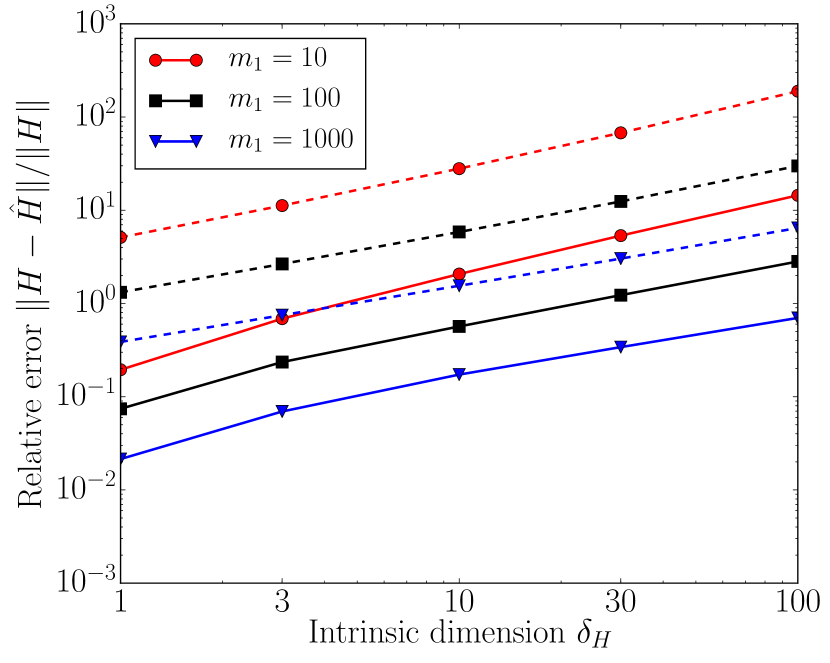
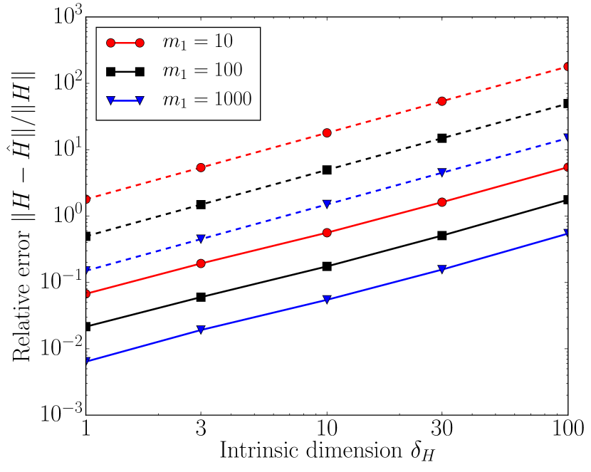
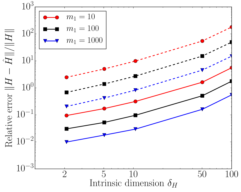
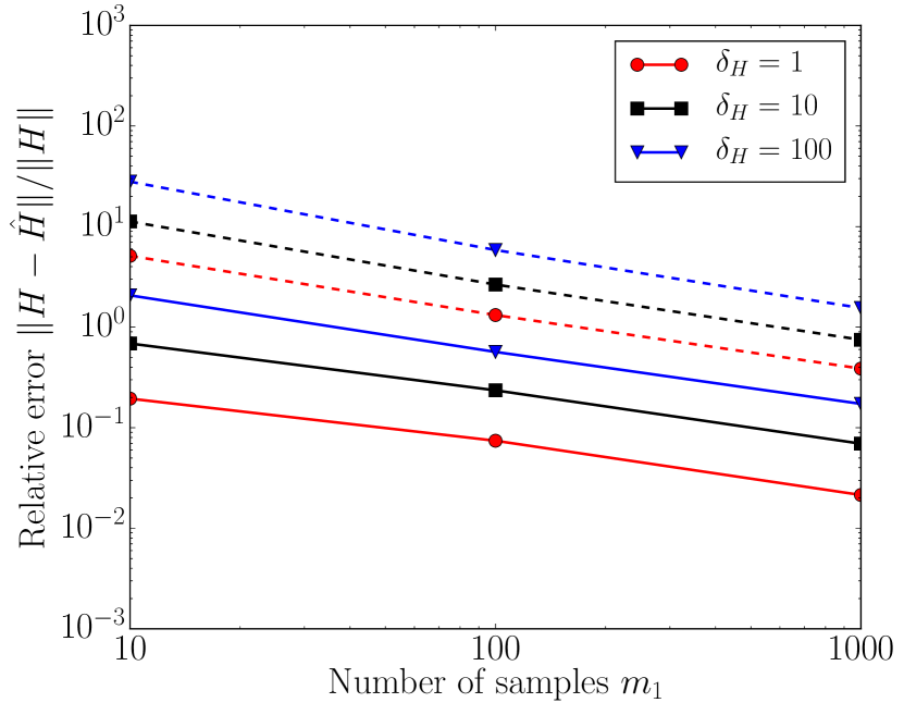
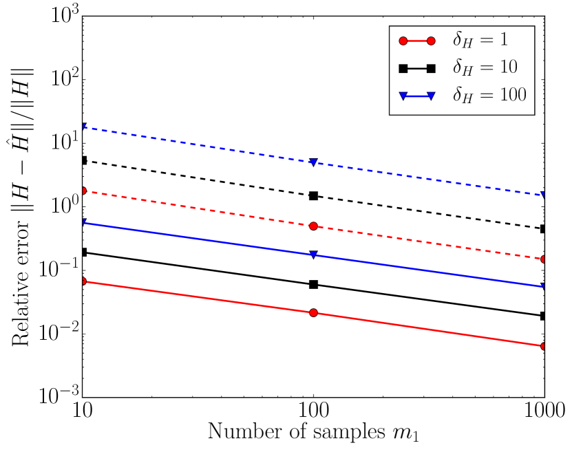
Figure 1 shows the average relative error of the SF estimator (left panel) and the MF estimator (right panel) as a function of the number of samples m1subscript𝑚1m_{1} for δH{1,10,100}subscript𝛿𝐻110100\delta_{H}\in\{1,10,100\}. The numerical results are in accordance with the theoretical bounds: the errors are dominated by the theoretical bounds and the slopes are similar. Comparing the left and right panels, we conclude that the MF estimator outperforms the SF estimator for a given number of high-fidelity evaluations. For example, in the case δH=1subscript𝛿𝐻1\delta_{H}=1, with m1=10subscript𝑚110m_{1}=10 high-fidelity samples, the MF estimator achieves a relative error of 0.07 while the SF relative error is 0.23—i.e., a relative error 3.47 times lower. Similarly, Figure 2 shows the average relative error as a function of the intrinsic dimension of H𝐻H for m1{10,100,1000}subscript𝑚1101001000m_{1}\in\{10,100,1000\}. We notice that the difference between the theoretical bound and the actual estimator error is larger for the MF estimator than for the SF estimator.
Refer to caption
Refer to caption
Figure 1: Rank-deficient example. Average relative error (solid line) as a function of the number of samples m1subscript𝑚1m_{1} for the SF estimator (left panel) and the MF estimator (right panel). Average is computed over 100 trials. Dashed lines represent theoretical bounds.
Refer to caption
Refer to caption
Figure 2: Rank-deficient example. Average relative error (solid line) as a function of the intrinsic dimension δHsubscript𝛿𝐻\delta_{H} for the SF estimator (left panel) and the MF estimator (right panel). Average is computed over 100 trials. Dashed lines represent theoretical bounds.

5.1.3 Full-rank matrices

In this section, we define the parameter 𝒂d𝒂superscript𝑑\boldsymbol{a}\in\mathbb{R}^{{\color[rgb]{0,0,0}\definecolor[named]{pgfstrokecolor}{rgb}{0,0,0}\pgfsys@color@gray@stroke{0}\pgfsys@color@gray@fill{0}d}} to be ai=exp(Ci),subscript𝑎𝑖𝐶𝑖a_{i}=\exp(-Ci), for all 1id1𝑖𝑑1\leq i\leq{\color[rgb]{0,0,0}\definecolor[named]{pgfstrokecolor}{rgb}{0,0,0}\pgfsys@color@gray@stroke{0}\pgfsys@color@gray@fill{0}d}, where the value of C0𝐶0C\geq 0 is set to match the intrinsic dimensions δH{2,5,10,50,100}.subscript𝛿𝐻251050100\delta_{H}\in\{2,5,10,50,100\}. The function f𝑓{\color[rgb]{0,0,0}\definecolor[named]{pgfstrokecolor}{rgb}{0,0,0}\pgfsys@color@gray@stroke{0}\pgfsys@color@gray@fill{0}f} now depends on every component of the input 𝒙𝒙{\color[rgb]{0,0,0}\definecolor[named]{pgfstrokecolor}{rgb}{0,0,0}\pgfsys@color@gray@stroke{0}\pgfsys@color@gray@fill{0}\boldsymbol{x}} and the matrix H𝐻H is full rank. Again, we study the dependence of the relative error H^H/Hnorm^𝐻𝐻norm𝐻\|\widehat{H}-H\|/\|H\| on the intrinsic dimension δHsubscript𝛿𝐻\delta_{H} and the number of samples m1subscript𝑚1m_{1}.

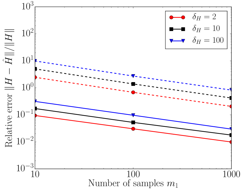
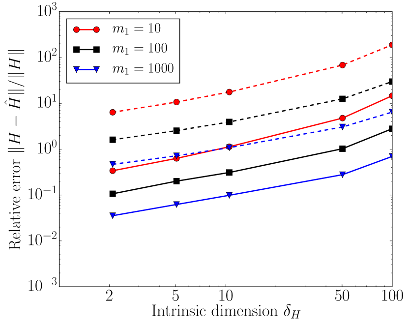
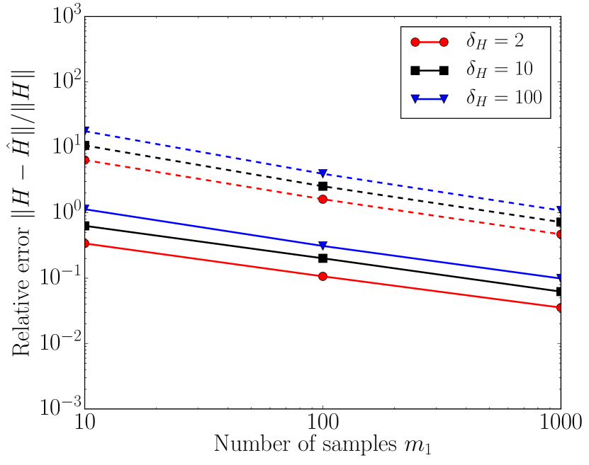
Figure 3 shows the average relative error of the SF estimator (left panel) and the MF estimator (right panel) as a function of the number of samples m1subscript𝑚1m_{1} for δH{2,10,100}subscript𝛿𝐻210100\delta_{H}\in\{2,10,100\}. The numerical results agree with the theoretical bounds: the errors are dominated by the theoretical bounds and the slopes are similar. Comparing the left and right panels, we conclude that the MF estimator outperforms the SF estimator for a given number of high-fidelity evaluations. For example, in the case δH=1subscript𝛿𝐻1\delta_{H}=1, with m1=10subscript𝑚110m_{1}=10 high-fidelity samples, the MF estimator achieves a relative error of 0.09 while the SF relative error is 0.37, leading to a relative error 3.86 times lower. Similarly, Figure 4 shows the average relative error as a function of the intrinsic dimension of H𝐻H for m1{10,100,1000}subscript𝑚1101001000m_{1}\in\{10,100,1000\}. Again, we observe that the empirical results satisfy the theoretical bounds.
Refer to caption
Refer to caption
Figure 3: Full-rank example. Average relative error (solid line) as a function of the number of samples m1subscript𝑚1m_{1} for the SF estimator (left panel) and the MF estimator (right panel). Average computed over 100 trials. Dashed lines represent theoretical bounds.
Refer to caption
Refer to caption
Figure 4: Full-rank example. Average relative error (solid line) as a function of the intrinsic dimension δHsubscript𝛿𝐻\delta_{H} for the SF estimator (left panel) and the MF estimator (right panel). Average computed over 100 trials. Dashed lines represent theoretical bounds.

5.2 Linear elasticity analysis of a wrench

We now demonstrate the proposed MF estimator on a high-dimensional engineering example.

5.2.1 Problem description

We consider a two-dimensional linear elasticity problem which consists of finding a smooth displacement field u:Ω2:𝑢Ωsuperscript2u:\Omega\rightarrow\mathbb{R}^{2} that satisfies

div(K:ε(u))=0 on Ω2,\text{div}(K:\varepsilon(u))=0\quad\text{ on }\Omega\subset\mathbb{R}^{2},

where ε(u)=12(u+uT)𝜀𝑢12𝑢superscript𝑢𝑇\varepsilon(u)=\frac{1}{2}(\nabla u+\nabla u^{T}) is the strain field and K𝐾K is the Hooke tensor. The boundary conditions are depicted in Figure 5(a). Using the plane stress assumption, the Hooke tensor K𝐾K satisfies

K:ε(u)=E1+νε(u)+νE1ν2trace(ε(u))I2,:𝐾𝜀𝑢𝐸1𝜈𝜀𝑢𝜈𝐸1superscript𝜈2trace𝜀𝑢subscript𝐼2K:\varepsilon(u)=\frac{E}{1+\nu}\varepsilon(u)+\frac{\nu E}{1-\nu^{2}}\operatorname{trace}(\varepsilon(u))I_{2},

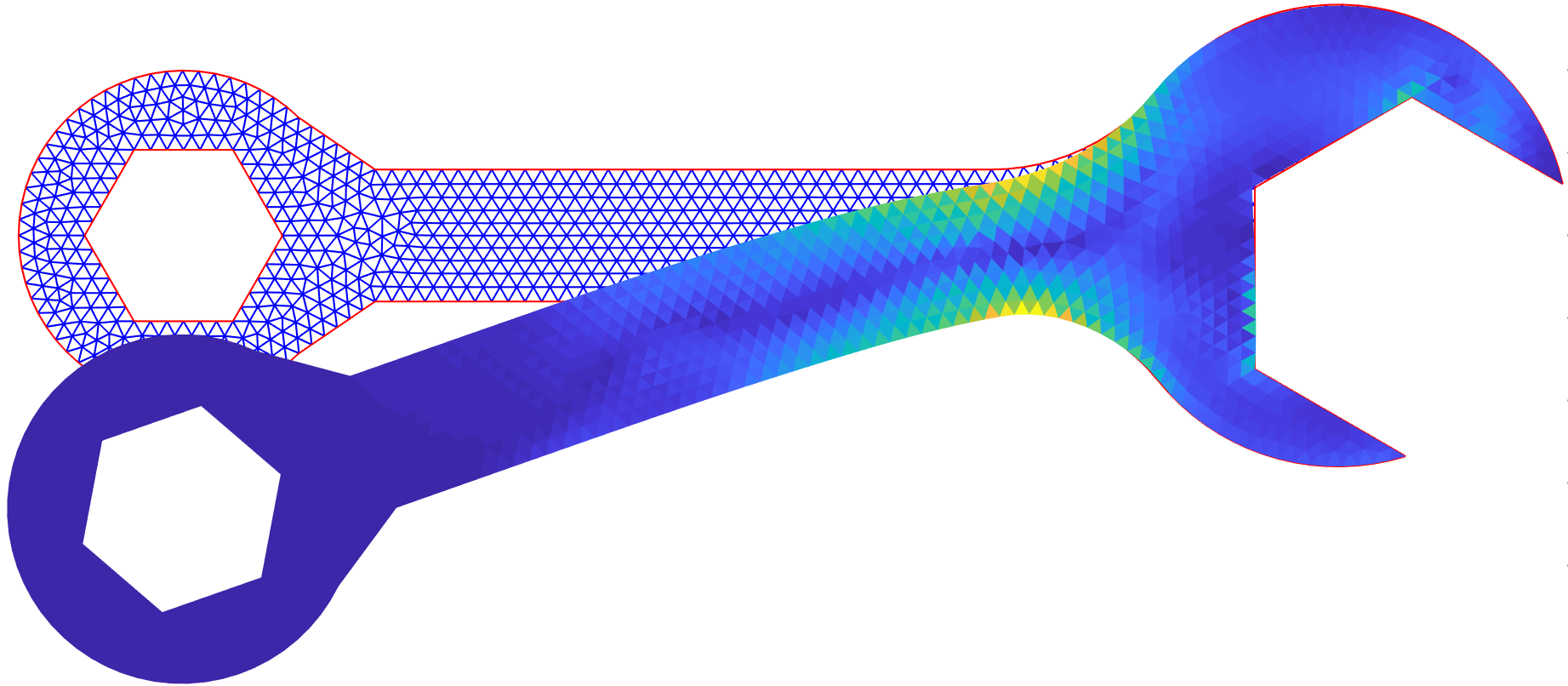
where ν=0.3𝜈0.3\nu=0.3 is the Poisson’s ratio and E0𝐸0E\geq 0 the Young’s modulus. We model E𝐸E as a random field such that log(E)𝒩(0,C)similar-to𝐸𝒩0𝐶\log(E)\sim\mathcal{N}(0,C) is a zero-mean Gaussian field over ΩΩ\Omega with covariance function C:Ω×Ω:𝐶ΩΩC:\Omega\times\Omega\rightarrow\mathbb{R} such that C(s,t)=exp(st22/l0)𝐶𝑠𝑡superscriptsubscriptnorm𝑠𝑡22subscript𝑙0C(s,t)=\exp(-\|s-t\|_{2}^{2}/l_{0}) with l0=1subscript𝑙01l_{0}=1. We consider the output defined by the vertical displacement of a point of interest (PoI) represented by the green point in Figure 5(a). We denote by u2(PoI)subscript𝑢2PoIu_{2}(\mathrm{PoI}) this scalar output, where the subscript ‘222’ refers to the vertical component of u𝑢u.

We denote by uhsuperscript𝑢u^{h} the finite element solution defined as the Galerkin projection of u𝑢u on a finite element space comprising continuous piecewise linear functions over the mesh depicted in Figure 5(b). To compute uhsuperscript𝑢u^{h}, we approximate the Young’s modulus log(E)𝐸\log(E) by a piecewise constant field log(Eh)superscript𝐸\log(E^{h}) that has the same statistics as log(E)𝐸\log(E) at the center of the elements. Denoting by d=2197𝑑2197{\color[rgb]{0,0,0}\definecolor[named]{pgfstrokecolor}{rgb}{0,0,0}\pgfsys@color@gray@stroke{0}\pgfsys@color@gray@fill{0}d}=2197 the number of elements in the mesh, we define f:d:𝑓superscript𝑑f:\mathbb{R}^{{\color[rgb]{0,0,0}\definecolor[named]{pgfstrokecolor}{rgb}{0,0,0}\pgfsys@color@gray@stroke{0}\pgfsys@color@gray@fill{0}d}}\rightarrow\mathbb{R} as the map from the log–Young’s modulus to the quantity of interest

f:X=log(Eh)u2h(PoI).:𝑓𝑋superscript𝐸maps-tosuperscriptsubscript𝑢2PoIf:X=\log(E^{h})\mapsto u_{2}^{h}(\mathrm{PoI}).
Refer to caption
(a) Geometry and boundary conditions.
Refer to caption
(b) Mesh and realization of uh(X)superscript𝑢𝑋u^{h}(X)
Figure 5: Left panel: Dirichlet condition u=0𝑢0u=0 (black chopped lines), vertical unitary linear forcing (red arrows), and point of interest PoIPoI\mathrm{PoI} (green dot). Right panel: mesh and finite element solution uh(X)superscript𝑢𝑋u^{h}(X) associated with one realization of X𝑋X, the random Young’s modulus. The color represents the von Mises stress.

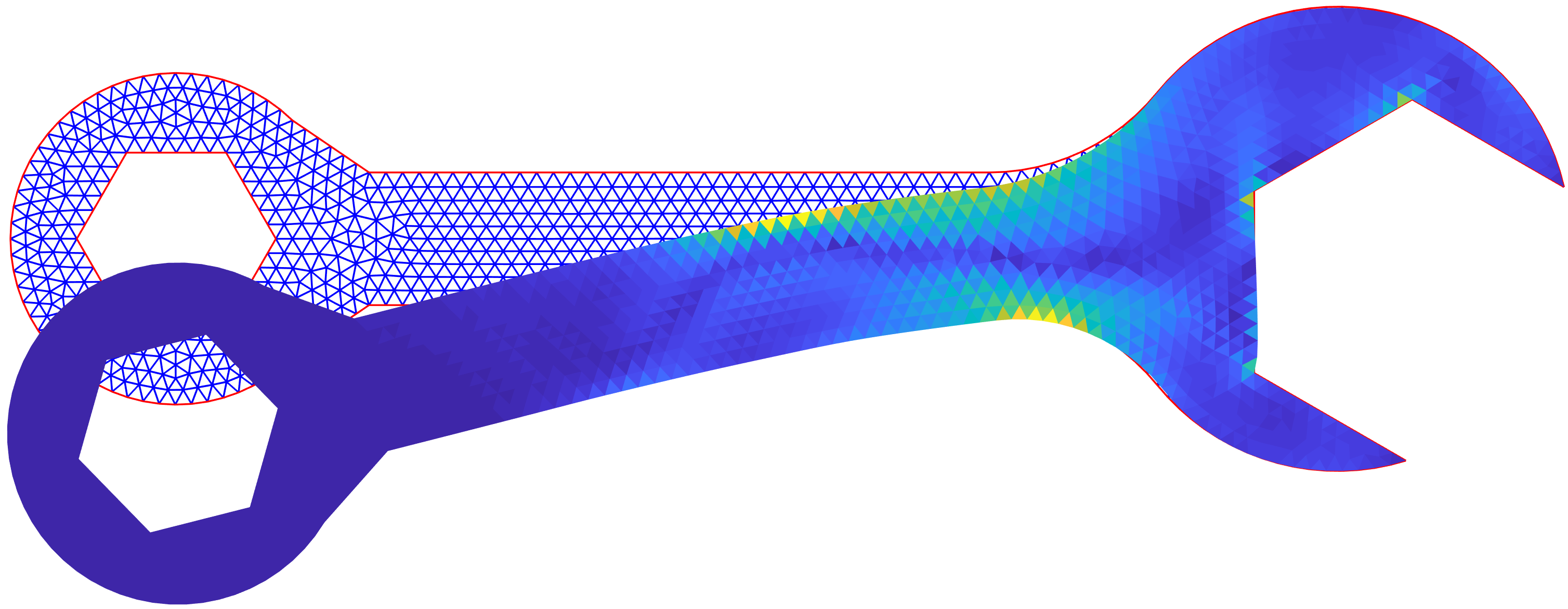
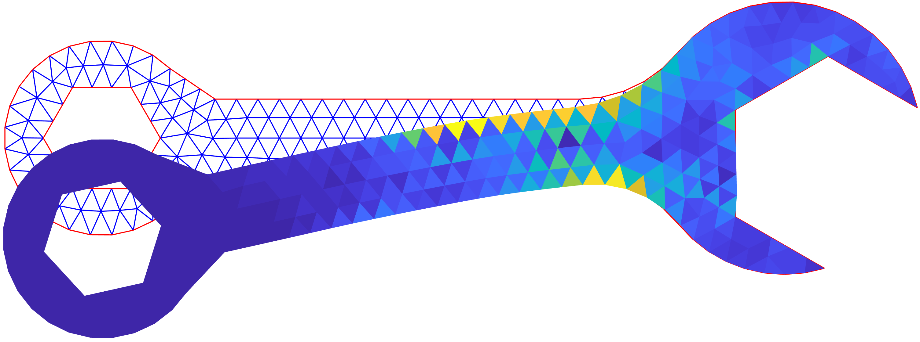
The gradients of f𝑓f are computed with the adjoint method; see for instance [31]. The complexity of computing the gradient increases with the number of elements in the mesh. For this reason, we introduce a low-fidelity model g𝑔g that relies on the coarser mesh depicted in Figure 6(d). This coarse mesh contains 423423423 elements, so that the function g𝑔g and its gradient can be evaluated with less computational effort compared to f𝑓f. We now explain in detail how g𝑔g is defined. First, the log of the Young’s modulus on the coarse mesh is defined as the piecewise constant field whose value at a given (coarse) element equals the spatial mean of X=log(Eh)𝑋superscript𝐸X=\log(E^{h}) restricted to that coarse element; see the illustration from Figure 6(a) to Figure 6(b). Then, we compute the coarse finite element solution and we define g(X)𝑔𝑋g(X) as the vertical displacement of the PoI. Figure 6(c) and Figure 6(d) show that the fine and coarse solutions are similar. With our implementation222Code available at https://gitlab.inria.fr/ozahm/wrenchmark.git., evaluating the gradient of the low-fidelity model g𝑔\nabla g is approximately 777 times faster than computing f𝑓\nabla f.

Refer to caption
(a) Realization of X=log(Eh)𝑋superscript𝐸X=\log(E^{h}) on the fine mesh
Refer to caption
(b) Projection of X𝑋X on the coarse mesh
Refer to caption
(c) Finite element solution on the fine mesh
Refer to caption
(d) Finite element solution on the coarse mesh
Figure 6: Construction of the low-fidelity approximation g𝑔g of f𝑓f using a coarse mesh. Figure 6(a) represents a realization of the Young’s modulus on the fine mesh and Figure 6(b) its projection onto the coarser mesh. The corresponding finite element solution on the fine mesh (resp. coarse) and von Mises stress are represented in Figure 6(c) (resp. Figure 6(d)).

Since the error bound (1) holds when X𝑋X is a standard Gaussian random vector, we employ the following change of variables. Denoting by ΣΣ\Sigma the covariance matrix of X𝒩(0,Σ)similar-to𝑋𝒩0ΣX\sim\mathcal{N}(0,\Sigma), we write X=Σ1/2Xstd𝑋superscriptΣ12subscript𝑋stdX=\Sigma^{1/2}X_{\text{std}} where Xstd𝒩(0,Id)similar-tosubscript𝑋std𝒩0subscript𝐼𝑑X_{\text{std}}\sim\mathcal{N}(0,I_{d}) and where Σ1/2superscriptΣ12\Sigma^{1/2} is a positive square root of ΣΣ\Sigma. After this change of variables, the high-fidelity and low-fidelity models are respectively fstd:Xstdf(Σ1/2Xstd):subscript𝑓stdmaps-tosubscript𝑋std𝑓superscriptΣ12subscript𝑋stdf_{\text{std}}:X_{\text{std}}\mapsto f(\Sigma^{1/2}X_{\text{std}}) and gstd:Xstdg(Σ1/2Xstd):subscript𝑔stdmaps-tosubscript𝑋std𝑔superscriptΣ12subscript𝑋stdg_{\text{std}}:X_{\text{std}}\mapsto g(\Sigma^{1/2}X_{\text{std}}) and the standardized AS matrix is Hstd=𝔼[fstd(Xstd)fstd(Xstd)T]subscript𝐻std𝔼delimited-[]subscript𝑓stdsubscript𝑋stdsubscript𝑓stdsuperscriptsubscript𝑋std𝑇H_{\text{std}}={\color[rgb]{0,0,0}\definecolor[named]{pgfstrokecolor}{rgb}{0,0,0}\pgfsys@color@gray@stroke{0}\pgfsys@color@gray@fill{0}\mathbb{E}}[\nabla f_{\text{std}}(X_{\text{std}})\nabla f_{\text{std}}(X_{\text{std}})^{T}]. This change of variable can be interpreted as a preconditioning step of the AS matrix H=𝔼[f(X)f(X)T]𝐻𝔼delimited-[]𝑓𝑋𝑓superscript𝑋𝑇H={\color[rgb]{0,0,0}\definecolor[named]{pgfstrokecolor}{rgb}{0,0,0}\pgfsys@color@gray@stroke{0}\pgfsys@color@gray@fill{0}\mathbb{E}}[\nabla f(X)\nabla f(X)^{T}] since we can write Hstd=ΣT/2HΣ1/2subscript𝐻stdsuperscriptΣ𝑇2𝐻superscriptΣ12H_{\text{std}}=\Sigma^{T/2}H\Sigma^{1/2}. For the sake of simplicity, we omit the subscript ‘std’ and we use the notations H𝐻H, f𝑓f, and g𝑔g for the standardized version of the AS matrix, the high-fidelity model, and low-fidelity model.

5.2.2 Numerical results

We compute 104superscript10410^{4} evaluations of the high-fidelity gradient f𝑓\nabla f and use them to form a SF estimator H^SFrefsuperscriptsubscript^𝐻𝑆𝐹ref\widehat{H}_{SF}^{\text{ref}} that we consider as a reference AS matrix. We compare the performance of the MF and SF estimators computed on ten cases characterized by different computational budgets. For a given case γ{1,,10}𝛾110\gamma\in\{1,\dots,10\}, the SF estimator is computed with m1=3γsubscript𝑚13𝛾m_{1}=3\gamma gradient evaluations while the MF estimator uses m1=2γsubscript𝑚12𝛾m_{1}=2\gamma and m2=5γsubscript𝑚25𝛾m_{2}=5\gamma. Given that evaluating g𝑔\nabla g is 7 times faster than evaluating f𝑓\nabla f, the computational costs of the SF and MF estimators are equivalent. In the following, we refer to γ𝛾\gamma as the cost coefficient, as we have set the computational budget to increase linearly with γ𝛾\gamma.

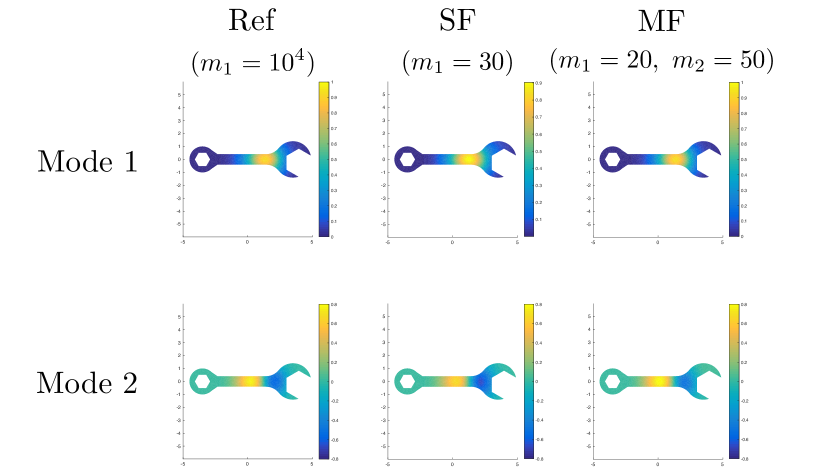
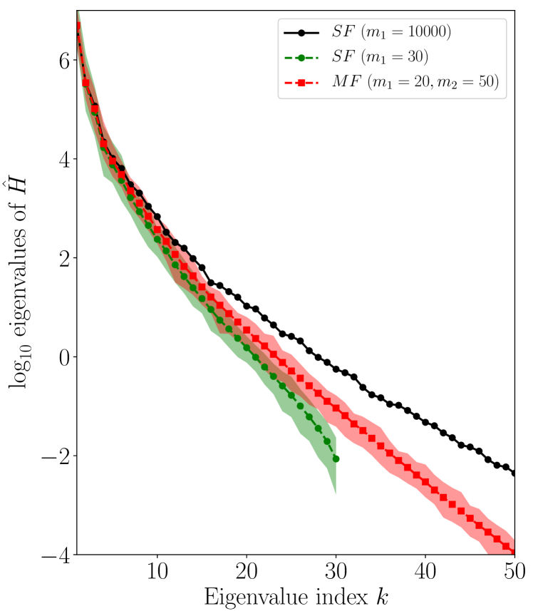
Figure 7 (left panel) shows the relative error with respect to the reference estimator H^SFrefsuperscriptsubscript^𝐻𝑆𝐹ref\widehat{H}_{SF}^{\text{ref}} as a function of the cost coefficient γ𝛾\gamma, averaged over 100 independent experiments. The MF estimator outperforms the SF estimator for all the budgets tested. In particular, the MF estimator (respectively SF estimator) reaches a relative error of 0.4 for γ=4𝛾4\gamma=4 (respectively γ=7𝛾7\gamma=7). This represents a 42.8%percent42.842.8\% reduction in computational resources for the MF estimator. Figure 7 (right panel) shows the eigenvalues of the AS matrix estimators, compared to those of the reference, for cost coefficient γ=10𝛾10\gamma=10. The MF estimator provides a better approximation of the spectral decay of the AS matrix than the SF estimator. We note that the spectral decay suggests that a few modes (5absent5\approx 5) are sufficient to describe the behavior of the function f𝑓{\color[rgb]{0,0,0}\definecolor[named]{pgfstrokecolor}{rgb}{0,0,0}\pgfsys@color@gray@stroke{0}\pgfsys@color@gray@fill{0}f}. Finally, Figure 8 shows the two leading modes (eigenvectors) from the reference, the SF, and the MF estimators for cost coefficient γ=10𝛾10\gamma=10. We note that both the SF and the MF estimators recover the leading modes correctly.
Refer to caption
Refer to caption
Figure 7: Left panel: Relative error as a function of cost coefficient γ𝛾\gamma, averaged over 100 independent experiments. At equivalent computational budget, the MF estimator outperforms the SF estimator. Right panel: Eigenvalues of the AS matrix estimators for the vertical displacement of the wrench PoI averaged over 100 independent experiments. Shadings represent the minimum and maximum values over the 100 independent experiments. The high-fidelity SF estimator used m1=30subscript𝑚130m_{1}=30 samples and the MF estimator is constructed with with m1=20subscript𝑚120m_{1}=20 and m2=50subscript𝑚250m_{2}=50 samples. This corresponds to a similar computational budget.
Refer to caption
Figure 8: First (top row) and second leading modes (bottom row) of the AS matrix for the reference estimator (left column), SF estimator (middle column) and MF estimator (right column) for the cost coefficient γ=10𝛾10\gamma=10. Both the SF and the MF estimators correctly capture the two leading modes of the reference AS matrix.

5.3 ONERA M6 wing shape optimization

In this section, we illustrate the proposed MF estimator on an expensive-to-evaluate engineering example.

We consider the problem of finding the active subspace associated with the shape optimization of the ONERA M6 wing. The shape of the wing is parameterized by free form deformation (FFD) box control points. In our experiment we used 5×8×2=80582805\times 8\times 2=80 FFD boxes. Imposing second-order continuity of surfaces with the FFD fixes 5×3×2=30532305\times 3\times 2=30 variables, leaving d=50𝑑50{\color[rgb]{0,0,0}\definecolor[named]{pgfstrokecolor}{rgb}{0,0,0}\pgfsys@color@gray@stroke{0}\pgfsys@color@gray@fill{0}d}=50 control points. These correspond to the input variable 𝒙𝒳=[0.05,0.05]50𝒙𝒳superscript0.050.0550{\color[rgb]{0,0,0}\definecolor[named]{pgfstrokecolor}{rgb}{0,0,0}\pgfsys@color@gray@stroke{0}\pgfsys@color@gray@fill{0}\boldsymbol{x}}\in\mathcal{X}=[-0.05,0.05]^{50}. The functions of interest are the drag and the lift coefficients. Those quantities are computed using expensive-to-evaluate computational fluid dynamics (CFD) tools. We use the SU2333https://github.com/su2code/SU2/tree/ec551e427f20373511432e6cd87402304cc46baa package [32] to solve the Reynolds-averaged Navier-Stokes (RANS) equations and compute the gradients using the continuous adjoint method. The flow conditions are such that the Mach number is M=0.8395subscript𝑀0.8395M_{\infty}=0.8395, the angle of attack of the wing is α=3.03°𝛼3.03°\alpha=$$, and the Reynolds number is Re=11.72×10⁶𝑅𝑒11.72superscript106Re=11.72\times 10^{6}. We use the Spalart-Allmaras turbulence model.

The high-fidelity function uses the aforementioned CFD model with the following stopping criteria: the solution of the RANS equations and the associated adjoint are computed with a limit of 104superscript10410^{4} iterations or fewer if the Cauchy convergence criteria reaches 105superscript10510^{-5} within this limit (i.e., maximum variation of the quantity of interest over 100 iterations is lower than 105superscript10510^{-5}). For the low-fidelity function g𝑔g, we use the same model as the high-fidelity function f𝑓{\color[rgb]{0,0,0}\definecolor[named]{pgfstrokecolor}{rgb}{0,0,0}\pgfsys@color@gray@stroke{0}\pgfsys@color@gray@fill{0}f} but reduce the maximum number of iterations allowed for convergence from 104superscript10410^{4} to 103superscript10310^{3}. An evaluation of the high-fidelity model (drag and lift coefficients and associated gradients) is thus approximately 101010 times more expensive than the low-fidelity model.

We compute a total of 100100100 high-fidelity evaluations and 500500500 low-fidelity evaluations. We use the 100 evaluations of the high-fidelity model to compute a first “reference” SF estimator (m1=100subscript𝑚1100m_{1}=100) that we denote H^SF(100)superscriptsubscript^𝐻𝑆𝐹100\widehat{H}_{SF}^{(100)}. We split the collected data into 5 independent experimental batches and construct three estimators per batch. The first is a SF estimator constructed with m1=10subscript𝑚110m_{1}=10 high-fidelity evaluations. The second is a SF estimator built with m1=20subscript𝑚120m_{1}=20 high-fidelity evaluations. The last estimator is a MF estimator with m1=10subscript𝑚110m_{1}=10 and m2=90subscript𝑚290m_{2}=90 evaluations. For these three estimators, the m1subscript𝑚1m_{1} high-fidelity evaluations are common. We note that the computational cost of the second SF estimator (m1=20subscript𝑚120m_{1}=20) and the MF estimator (m1=10subscript𝑚110m_{1}=10 and m2=90subscript𝑚290m_{2}=90) are similar.

Refer to caption
Refer to caption
Figure 9: Eigenvalues of the AS matrix estimators for the drag coefficient (left panel) and for the lift coefficient (right panel) averaged over 5 independent experiments. The SF estimator with m1=20subscript𝑚120m_{1}=20 and the MF estimator (dashed lines) used the same computational budget to evaluate the gradients. At equal budget, the MF estimator provides a better estimate of the spectrum of H^SF(100)superscriptsubscript^𝐻𝑆𝐹100\widehat{H}_{SF}^{(100)} than the SF estimator. Shadings represent maximum and minimum values over the 5 independent experiments.
Refer to caption
Refer to caption
Figure 10: Eigenvalues of the AS matrix estimators for the drag coefficient (left panel) and for the lift coefficient (right panel). The high-fidelity SF estimator used m1=100subscript𝑚1100m_{1}=100 samples and the MF estimator is constructed with with m1=100subscript𝑚1100m_{1}=100 and m2=400subscript𝑚2400m_{2}=400 samples.

Figure 9 shows the 20 first eigenvalues of the three estimators (averaged over 5 independent batches) and H^SF(100)superscriptsubscript^𝐻𝑆𝐹100\widehat{H}_{SF}^{(100)}. Note that the SF estimators (except H^SF(100)superscriptsubscript^𝐻𝑆𝐹100\widehat{H}_{SF}^{(100)}) are rank deficient (rank 10 and rank 20). The MF estimator is full rank (rank 50). The MF estimator is closer to H^SF(100)superscriptsubscript^𝐻𝑆𝐹100\widehat{H}_{SF}^{(100)} than the two SF estimators. In particular, the MF estimator outperforms the second SF estimator with similar computational budget. The error bars show the maximum and the minimum values over the 5 independent experiments for each estimator and confirm the robustness of the proposed method.

Figure 10 shows the 50 eigenvalues of the SF estimator H^SF(100)superscriptsubscript^𝐻𝑆𝐹100\widehat{H}_{SF}^{(100)} (m1=100subscript𝑚1100m_{1}=100) and a MF estimator using all the available evaluations (m1=100subscript𝑚1100m_{1}=100, m2=400subscript𝑚2400m_{2}=400). The leading eigenvalues are similar for both estimators. The difference between the two estimators increases for lower eigenvalues (higher indices). For both estimators, we compute approximations of the characteristic quantities δHsubscript𝛿𝐻\delta_{H}, 𝔼[f(X)2]𝔼delimited-[]superscriptnorm𝑓𝑋2{\color[rgb]{0,0,0}\definecolor[named]{pgfstrokecolor}{rgb}{0,0,0}\pgfsys@color@gray@stroke{0}\pgfsys@color@gray@fill{0}\mathbb{E}}[\|\nabla f(X)\|^{2}], Hnorm𝐻\|H\|, β2superscript𝛽2\beta^{2}, and θ2superscript𝜃2\theta^{2} and summarize them in Table 1. The SF quantities are computed based on the m1=100subscript𝑚1100m_{1}=100 high-fidelity evaluations: Hnorm𝐻\|H\| and δHsubscript𝛿𝐻\delta_{H} are computed using H^SF(100)superscriptsubscript^𝐻𝑆𝐹100\widehat{H}_{SF}^{(100)} in lieu of H𝐻H, 𝔼[f(X)2]𝔼delimited-[]superscriptnorm𝑓𝑋2{\color[rgb]{0,0,0}\definecolor[named]{pgfstrokecolor}{rgb}{0,0,0}\pgfsys@color@gray@stroke{0}\pgfsys@color@gray@fill{0}\mathbb{E}}[\|\nabla f(X)\|^{2}] is approximated by 1m1i=1m1f(Xi)21subscript𝑚1superscriptsubscript𝑖1subscript𝑚1superscriptnorm𝑓subscript𝑋𝑖2\frac{1}{m_{1}}\sum_{i=1}^{m_{1}}\|\nabla f(X_{i})\|^{2}, while β2superscript𝛽2\beta^{2} is approximated by maxif(Xi)2/𝔼[f(X)2]subscript𝑖superscriptnorm𝑓subscript𝑋𝑖2𝔼delimited-[]superscriptnorm𝑓𝑋2\max_{i}\|\nabla f(X_{i})\|^{2}/{\color[rgb]{0,0,0}\definecolor[named]{pgfstrokecolor}{rgb}{0,0,0}\pgfsys@color@gray@stroke{0}\pgfsys@color@gray@fill{0}\mathbb{E}}[\|\nabla f(X)\|^{2}] for i{1,,m1}𝑖1subscript𝑚1i\in\{1,\dots,m_{1}\}. The MF quantities are computed based on the m1=100subscript𝑚1100m_{1}=100 high-fidelity evaluations and m1+m2=500subscript𝑚1subscript𝑚2500m_{1}+m_{2}=500 low-fidelity evaluations: Hnorm𝐻\|H\| and δHsubscript𝛿𝐻\delta_{H} are computed using the MF estimator in lieu of H𝐻H, 𝔼[f(X)2]𝔼delimited-[]superscriptnorm𝑓𝑋2{\color[rgb]{0,0,0}\definecolor[named]{pgfstrokecolor}{rgb}{0,0,0}\pgfsys@color@gray@stroke{0}\pgfsys@color@gray@fill{0}\mathbb{E}}[\|\nabla f(X)\|^{2}] is approximated by the (scalar) MF estimator 1m1i=1m1(f(Xi)2g(Xi)2)+1m2i=m1+1m1+m2g(Xi)21subscript𝑚1superscriptsubscript𝑖1subscript𝑚1superscriptnorm𝑓subscript𝑋𝑖2superscriptnorm𝑔subscript𝑋𝑖21subscript𝑚2superscriptsubscript𝑖subscript𝑚11subscript𝑚1subscript𝑚2superscriptnorm𝑔subscript𝑋𝑖2\frac{1}{m_{1}}\sum_{i=1}^{m_{1}}(\|\nabla f(X_{i})\|^{2}-\|\nabla g(X_{i})\|^{2})+\frac{1}{m_{2}}\sum_{i=m_{1}+1}^{m_{1}+m_{2}}\|\nabla g(X_{i})\|^{2}, while θ2superscript𝜃2\theta^{2} is approximated by maxif(Xi)g(Xi)2/𝔼[f(X)2]subscript𝑖superscriptnorm𝑓subscript𝑋𝑖𝑔subscript𝑋𝑖2𝔼delimited-[]superscriptnorm𝑓𝑋2\max_{i}\|\nabla f(X_{i})-\nabla g(X_{i})\|^{2}/{\color[rgb]{0,0,0}\definecolor[named]{pgfstrokecolor}{rgb}{0,0,0}\pgfsys@color@gray@stroke{0}\pgfsys@color@gray@fill{0}\mathbb{E}}[\|\nabla f(X)\|^{2}] for i{1,,m1}𝑖1subscript𝑚1i\in\{1,\dots,m_{1}\}.

Table 1: Approximation of the characteristic quantities for the SF and MF estimators for the drag and lift coefficients.
Drag coefficient Cdsubscript𝐶𝑑C_{d} Lift coefficient Clsubscript𝐶𝑙C_{l}
SF MF SF MF
𝔼[f(X)2]𝔼delimited-[]superscriptnorm𝑓𝑋2{\color[rgb]{0,0,0}\definecolor[named]{pgfstrokecolor}{rgb}{0,0,0}\pgfsys@color@gray@stroke{0}\pgfsys@color@gray@fill{0}\mathbb{E}}[\|\nabla f(X)\|^{2}] 1.74×1051.74superscript1051.74\times 10^{-5} 1.81×1051.81superscript1051.81\times 10^{-5} 5.96×1035.96superscript1035.96\times 10^{-3} 6.08×1036.08superscript1036.08\times 10^{-3}
Hnorm𝐻\|H\| 2.09×1062.09superscript1062.09\times 10^{-6} 1.99×1061.99superscript1061.99\times 10^{-6} 6.16×1046.16superscript1046.16\times 10^{-4} 6.38×1046.38superscript1046.38\times 10^{-4}
δHsubscript𝛿𝐻\delta_{H} 8.34 9.10 9.67 9.53
β2superscript𝛽2\beta^{2} 1.76 - 1.54 -
θ2superscript𝜃2\theta^{2} - 1.30×1051.30superscript1051.30\times 10^{-5} - 1.03×1041.03superscript1041.03\times 10^{-4}

From Table 1, it can be seen that the intrinsic dimension of the AS matrix is approximately 9 for both the drag and lift coefficients. Table 1 also shows that the parameter β2superscript𝛽2\beta^{2} is not large (2absent2\leq 2), which indicates, along with the low intrinsic dimension, that computing a good estimator of H𝐻H requires relatively few evaluations. We also note that the low-fidelity model is a good approximation of the high-fidelity model, with θ21.5×10⁵superscript𝜃21.5superscript105\theta^{2}\leq 1.5\times 10^{-5} for the drag and θ21.1×10⁴superscript𝜃21.1superscript104\theta^{2}\leq 1.1\times 10^{-4} for the lift. Figure 11 shows the normalized sum of the eigenvalues of the best rank-r𝑟r approximation of H^^𝐻\widehat{H}. Selecting the 20 first eigenvectors of H^^𝐻\widehat{H} allows us to capture more than 80% of the spectral content and decreases by 30 the dimensionality of the shape optimization problem (a 60%percent6060\% decrease).

Refer to caption
Figure 11: Percentage of the spectrum k=1iλr(H^)/tr(H^)superscriptsubscript𝑘1𝑖subscript𝜆𝑟^𝐻𝑡𝑟^𝐻\sum_{k=1}^{i}\lambda_{r}(\widehat{H})/tr(\widehat{H}) captured by the best rank-r𝑟r approximation of H^^𝐻\widehat{H}, where λk(H^)subscript𝜆𝑘^𝐻\lambda_{k}(\widehat{H}) is the kthsuperscript𝑘𝑡k^{th} eigenvalue of H^^𝐻\widehat{H}.

6 Conclusions

We proposed a multifidelity approach to identify low-dimensional subspaces capturing most of the variation of a function of interest. Our approach builds on the gradient-based active subspace methodology, which seeks to compute the matrix H𝐻H containing the second moments of the gradient function. The proposed approach reduces the computational cost of Monte Carlo methods used to estimate this matrix, by using a low-fidelity, cheap-to-evaluate gradient approximation as a control variate. The performance improvements of the resulting multifidelity (MF) estimator H^MFsubscript^𝐻𝑀𝐹\widehat{H}_{MF} are demonstrated on two engineering examples governed by partial differential equations: a high-dimensional linear elasticity problem defined over more than two thousand input variables and an expensive shape optimization problem defined over 50 input variables.

Analysis of the performance of the multifidelity technique yields error bounds for the matrix error HH^MFnorm𝐻subscript^𝐻𝑀𝐹\|H-\widehat{H}_{MF}\| both in expectation and with high probability. These error bounds depend on the intrinsic dimension of the problem, which is related to the spectral decay of the active subspace matrix. When a function varies mostly along a few directions, the intrinsic dimension is low. In such a case, approximating H𝐻H may require only a small number of gradient evaluations. This relationship was confirmed empirically by a parametric study conducted on two analytical problems: lower intrinsic dimension led to lower matrix error for the same number of high-fidelity evaluations.

The performance improvements of the multifidelity approach are threefold. First, we showed that the MF estimator reduces the cost of performing dimension reduction. This was illustrated on the linear elasticity problem, where the multifidelity approach needed about 43%percent4343\% less computational effort than its single-fidelity counterpart to achieve the same relative error. Second, we showed that the multifidelity approach was able to recover eigenvectors qualitatively similar to the exact ones. Third, the MF estimator led to better estimates of the spectral decay of H𝐻H. On the linear elasticity problem, which is characterized by a low intrinsic dimension (5absent5\leq 5), the multifidelity approach led to better estimates, especially for smaller eigenvalues. On the shape optimization problem, which is characterized by a higher intrinsic dimension (9absent9\approx 9), the MF estimator led to better estimates for all eigenvalues. This behavior is in contrast to the single-fidelity method, which overestimated the leading eigenvalues and underestimated the lower eigenvalues, thereby underestimating the intrinsic dimension of H𝐻H and overestimating the spectral decay. Recovering the spectral decay of H𝐻H is particularly important since one popular way of choosing the dimension r𝑟r of the active subspace is based on the spectral gap between consecutive eigenvalues. If the spectral decay is overestimated, r𝑟r might be chosen too small to correctly capture the behavior of the high-fidelity function. By providing a better estimate of the spectral decay, the MF estimator reduces this risk.

The dimension of the active subspace can also be chosen to control an error bound on the associated function approximation error, i.e., when using the active subspace to construct a ridge approximation of the original function. We showed that the approximation of this bound, which depends on the unknown H𝐻H, improves as the matrix error decreases. Because the MF estimator reduces the error in estimating H𝐻H for a given computational effort, the proposed multifidelity approach leads to a better selection of the active subspace dimension r𝑟r.

Appendix A Proofs of main results

In this section, we present the details of the proofs of Proposition 4.1 (Appendix A.1) and Proposition 4.3 (Appendix A.2).

A.1 Proof of Proposition 4.1

The proof of Proposition 4.1 relies on the concentration inequality known as the matrix Bernstein theorem. It corresponds to Theorem 6.1.1 from [47] restricted to the case of real symmetric matrices.

Theorem A.1 (Matrix Bernstein: real symmetric case [47]).

Let S1,,Smsubscript𝑆1subscript𝑆𝑚S_{1},\ldots,S_{m} be m𝑚m independent zero-mean random symmetric matrices in d×dsuperscript𝑑𝑑\mathbb{R}^{{\color[rgb]{0,0,0}\definecolor[named]{pgfstrokecolor}{rgb}{0,0,0}\pgfsys@color@gray@stroke{0}\pgfsys@color@gray@fill{0}d}\times{\color[rgb]{0,0,0}\definecolor[named]{pgfstrokecolor}{rgb}{0,0,0}\pgfsys@color@gray@stroke{0}\pgfsys@color@gray@fill{0}d}}. Assume there exists L<𝐿L<\infty such that

SiL,normsubscript𝑆𝑖𝐿\displaystyle\|S_{i}\|\leq L,

almost surely for all 1im1𝑖𝑚1\leq i\leq m, and let v𝑣v be such that

𝔼[(S1++Sm)2]v.norm𝔼delimited-[]superscriptsubscript𝑆1subscript𝑆𝑚2𝑣\|{\color[rgb]{0,0,0}\definecolor[named]{pgfstrokecolor}{rgb}{0,0,0}\pgfsys@color@gray@stroke{0}\pgfsys@color@gray@fill{0}\mathbb{E}}[(S_{1}+\ldots+S_{m})^{2}]\|\leq v.

Then,

𝔼[S1++Sm]𝔼delimited-[]normsubscript𝑆1subscript𝑆𝑚\displaystyle{\color[rgb]{0,0,0}\definecolor[named]{pgfstrokecolor}{rgb}{0,0,0}\pgfsys@color@gray@stroke{0}\pgfsys@color@gray@fill{0}\mathbb{E}}[\|S_{1}+\ldots+S_{m}\|] 2vlog(2d)+13Llog(2d).absent2𝑣2𝑑13𝐿2𝑑\displaystyle\leq\sqrt{2v\log(2{\color[rgb]{0,0,0}\definecolor[named]{pgfstrokecolor}{rgb}{0,0,0}\pgfsys@color@gray@stroke{0}\pgfsys@color@gray@fill{0}d})}+\frac{1}{3}L\log(2d).

Furthermore, for any t0𝑡0t\geq 0 we have

{S1++Smt}2dexp(t2/2v+Lt/3).normsubscript𝑆1subscript𝑆𝑚𝑡2𝑑superscript𝑡22𝑣𝐿𝑡3\displaystyle\mathbb{P}\{\|S_{1}+\ldots+S_{m}\|\geq t\}\leq 2{\color[rgb]{0,0,0}\definecolor[named]{pgfstrokecolor}{rgb}{0,0,0}\pgfsys@color@gray@stroke{0}\pgfsys@color@gray@fill{0}d}\exp\left(\frac{-t^{2}/2}{v+Lt/3}\right).

In order to apply the matrix Bernstein theorem, we need to express the difference between the AS matrix H𝐻H and the MF estimator H^MFsubscript^𝐻𝑀𝐹\widehat{H}_{MF} as the sum of independent matrices. We write HH^MF=S1++Sm,𝐻subscript^𝐻𝑀𝐹subscript𝑆1subscript𝑆𝑚H-\widehat{H}_{MF}=S_{1}+\ldots+S_{m}, where m=m1+m2𝑚subscript𝑚1subscript𝑚2m=m_{1}+m_{2} and

Si={1m1(HG(f(X)f(X)Tg(X)g(X)T)),if 1im1,1m2(Gg(X)g(X)T).otherwise,subscript𝑆𝑖cases1subscript𝑚1𝐻𝐺𝑓𝑋𝑓superscript𝑋𝑇𝑔𝑋𝑔superscript𝑋𝑇if 1𝑖subscript𝑚11subscript𝑚2𝐺𝑔𝑋𝑔superscript𝑋𝑇otherwiseS_{i}=\left\{\begin{array}[]{ll}\frac{1}{m_{1}}\big{(}H-G-(\nabla f(X)\nabla f(X)^{T}-\nabla g(X)\nabla g(X)^{T})\big{)},&\text{if }1\leq i\leq m_{1},\\ \frac{1}{m_{2}}\big{(}G-\nabla g(X)\nabla g(X)^{T}\big{)}.&\text{otherwise},\end{array}\right.

where G=𝔼[g(X)g(X)T]𝐺𝔼delimited-[]𝑔𝑋𝑔superscript𝑋𝑇G={\color[rgb]{0,0,0}\definecolor[named]{pgfstrokecolor}{rgb}{0,0,0}\pgfsys@color@gray@stroke{0}\pgfsys@color@gray@fill{0}\mathbb{E}}[\nabla g(X)\nabla g(X)^{T}]. The following property provides bounds for Sinormsubscript𝑆𝑖\|S_{i}\| and 𝔼[S1++Sm]𝔼delimited-[]normsubscript𝑆1subscript𝑆𝑚{\color[rgb]{0,0,0}\definecolor[named]{pgfstrokecolor}{rgb}{0,0,0}\pgfsys@color@gray@stroke{0}\pgfsys@color@gray@fill{0}\mathbb{E}}[\|S_{1}+\ldots+S_{m}\|]. Those bounds are expressed as functions of m1subscript𝑚1m_{1}, m2subscript𝑚2m_{2}, β𝛽\beta, θ𝜃\theta, and 𝔼[f(X)2]𝔼delimited-[]superscriptnorm𝑓𝑋2{\color[rgb]{0,0,0}\definecolor[named]{pgfstrokecolor}{rgb}{0,0,0}\pgfsys@color@gray@stroke{0}\pgfsys@color@gray@fill{0}\mathbb{E}}[\|\nabla f(X)\|^{2}].

Property A.2.

Assumptions (10) and (11) yield

(22) 𝔼[(S1++Sm)2](θ2(2+θ)2m1+(θ+β)2(1+θ)2m2)𝔼[f(X)2]2,norm𝔼delimited-[]superscriptsubscript𝑆1subscript𝑆𝑚2superscript𝜃2superscript2𝜃2subscript𝑚1superscript𝜃𝛽2superscript1𝜃2subscript𝑚2𝔼superscriptdelimited-[]superscriptnorm𝑓𝑋22\|{\color[rgb]{0,0,0}\definecolor[named]{pgfstrokecolor}{rgb}{0,0,0}\pgfsys@color@gray@stroke{0}\pgfsys@color@gray@fill{0}\mathbb{E}}[(S_{1}+\ldots+S_{m})^{2}]\|\leq\left(\frac{\theta^{2}(2+\theta)^{2}}{m_{1}}+\frac{(\theta+\beta)^{2}(1+\theta)^{2}}{m_{2}}\right){\color[rgb]{0,0,0}\definecolor[named]{pgfstrokecolor}{rgb}{0,0,0}\pgfsys@color@gray@stroke{0}\pgfsys@color@gray@fill{0}\mathbb{E}}[\|\nabla f(X)\|^{2}]^{2},

and

(23) Simax{2θ(2β+θ)m1;2(θ+β)2m2}𝔼[f(X)2].normsubscript𝑆𝑖max2𝜃2𝛽𝜃subscript𝑚12superscript𝜃𝛽2subscript𝑚2𝔼delimited-[]superscriptnorm𝑓𝑋2\|S_{i}\|\leq\operatorname{max}\left\{\frac{2\theta(2\beta+\theta)}{m_{1}};\frac{2(\theta+\beta)^{2}}{m_{2}}\right\}{\color[rgb]{0,0,0}\definecolor[named]{pgfstrokecolor}{rgb}{0,0,0}\pgfsys@color@gray@stroke{0}\pgfsys@color@gray@fill{0}\mathbb{E}}[\|\nabla f(X)\|^{2}].

almost surely for all 1im1𝑖𝑚1\leq i\leq m.

Proof A.3.

We first derive the bound (22) for the variance of the estimator before proving the bound (23) for the norm of the summands.

Using the independence of the summands Sisubscript𝑆𝑖S_{i} and the fact that 𝔼[Si]=0𝔼delimited-[]subscript𝑆𝑖0{\color[rgb]{0,0,0}\definecolor[named]{pgfstrokecolor}{rgb}{0,0,0}\pgfsys@color@gray@stroke{0}\pgfsys@color@gray@fill{0}\mathbb{E}}[S_{i}]=0, we have

𝔼[(S1++Sm)2]𝔼delimited-[]superscriptsubscript𝑆1subscript𝑆𝑚2\displaystyle{\color[rgb]{0,0,0}\definecolor[named]{pgfstrokecolor}{rgb}{0,0,0}\pgfsys@color@gray@stroke{0}\pgfsys@color@gray@fill{0}\mathbb{E}}[(S_{1}+\ldots+S_{m})^{2}] =𝔼[S12]++𝔼[Sm12]+𝔼[Sm1+12]++𝔼[Sm2]absent𝔼delimited-[]superscriptsubscript𝑆12𝔼delimited-[]superscriptsubscript𝑆subscript𝑚12𝔼delimited-[]superscriptsubscript𝑆subscript𝑚112𝔼delimited-[]superscriptsubscript𝑆𝑚2\displaystyle={\color[rgb]{0,0,0}\definecolor[named]{pgfstrokecolor}{rgb}{0,0,0}\pgfsys@color@gray@stroke{0}\pgfsys@color@gray@fill{0}\mathbb{E}}[S_{1}^{2}]+\ldots+{\color[rgb]{0,0,0}\definecolor[named]{pgfstrokecolor}{rgb}{0,0,0}\pgfsys@color@gray@stroke{0}\pgfsys@color@gray@fill{0}\mathbb{E}}[S_{m_{1}}^{2}]+{\color[rgb]{0,0,0}\definecolor[named]{pgfstrokecolor}{rgb}{0,0,0}\pgfsys@color@gray@stroke{0}\pgfsys@color@gray@fill{0}\mathbb{E}}[S_{m_{1}+1}^{2}]+\ldots+{\color[rgb]{0,0,0}\definecolor[named]{pgfstrokecolor}{rgb}{0,0,0}\pgfsys@color@gray@stroke{0}\pgfsys@color@gray@fill{0}\mathbb{E}}[S_{m}^{2}]
(24) =1m1𝔼[(A𝔼[A])2]+1m2𝔼[(B𝔼[B])2],absent1subscript𝑚1𝔼delimited-[]superscript𝐴𝔼delimited-[]𝐴21subscript𝑚2𝔼delimited-[]superscript𝐵𝔼delimited-[]𝐵2\displaystyle=\frac{1}{m_{1}}{\color[rgb]{0,0,0}\definecolor[named]{pgfstrokecolor}{rgb}{0,0,0}\pgfsys@color@gray@stroke{0}\pgfsys@color@gray@fill{0}\mathbb{E}}[(A-{\color[rgb]{0,0,0}\definecolor[named]{pgfstrokecolor}{rgb}{0,0,0}\pgfsys@color@gray@stroke{0}\pgfsys@color@gray@fill{0}\mathbb{E}}[A])^{2}]+\frac{1}{m_{2}}{\color[rgb]{0,0,0}\definecolor[named]{pgfstrokecolor}{rgb}{0,0,0}\pgfsys@color@gray@stroke{0}\pgfsys@color@gray@fill{0}\mathbb{E}}[(B-{\color[rgb]{0,0,0}\definecolor[named]{pgfstrokecolor}{rgb}{0,0,0}\pgfsys@color@gray@stroke{0}\pgfsys@color@gray@fill{0}\mathbb{E}}[B])^{2}],

where

A𝐴\displaystyle A =f(X)f(X)Tg(X)g(X)T,absent𝑓𝑋𝑓superscript𝑋𝑇𝑔𝑋𝑔superscript𝑋𝑇\displaystyle=\nabla f(X)\nabla f(X)^{T}-\nabla g(X)\nabla g(X)^{T},
B𝐵\displaystyle B =g(X)g(X)T.absent𝑔𝑋𝑔superscript𝑋𝑇\displaystyle=\nabla g(X)\nabla g(X)^{T}.

Notice that 0𝔼[(A𝔼[A])2]=𝔼[A2]𝔼[A]2𝔼[A2]precedes-or-equals0𝔼delimited-[]superscript𝐴𝔼delimited-[]𝐴2𝔼delimited-[]superscript𝐴2𝔼superscriptdelimited-[]𝐴2precedes-or-equals𝔼delimited-[]superscript𝐴20\preccurlyeq{\color[rgb]{0,0,0}\definecolor[named]{pgfstrokecolor}{rgb}{0,0,0}\pgfsys@color@gray@stroke{0}\pgfsys@color@gray@fill{0}\mathbb{E}}[(A-{\color[rgb]{0,0,0}\definecolor[named]{pgfstrokecolor}{rgb}{0,0,0}\pgfsys@color@gray@stroke{0}\pgfsys@color@gray@fill{0}\mathbb{E}}[A])^{2}]={\color[rgb]{0,0,0}\definecolor[named]{pgfstrokecolor}{rgb}{0,0,0}\pgfsys@color@gray@stroke{0}\pgfsys@color@gray@fill{0}\mathbb{E}}[A^{2}]-{\color[rgb]{0,0,0}\definecolor[named]{pgfstrokecolor}{rgb}{0,0,0}\pgfsys@color@gray@stroke{0}\pgfsys@color@gray@fill{0}\mathbb{E}}[A]^{2}\preccurlyeq{\color[rgb]{0,0,0}\definecolor[named]{pgfstrokecolor}{rgb}{0,0,0}\pgfsys@color@gray@stroke{0}\pgfsys@color@gray@fill{0}\mathbb{E}}[A^{2}] so that 𝔼[(A𝔼[A])2]𝔼[A2]norm𝔼delimited-[]superscript𝐴𝔼delimited-[]𝐴2norm𝔼delimited-[]superscript𝐴2\|{\color[rgb]{0,0,0}\definecolor[named]{pgfstrokecolor}{rgb}{0,0,0}\pgfsys@color@gray@stroke{0}\pgfsys@color@gray@fill{0}\mathbb{E}}[(A-{\color[rgb]{0,0,0}\definecolor[named]{pgfstrokecolor}{rgb}{0,0,0}\pgfsys@color@gray@stroke{0}\pgfsys@color@gray@fill{0}\mathbb{E}}[A])^{2}]\|\leq\|{\color[rgb]{0,0,0}\definecolor[named]{pgfstrokecolor}{rgb}{0,0,0}\pgfsys@color@gray@stroke{0}\pgfsys@color@gray@fill{0}\mathbb{E}}[A^{2}]\|, where precedes-or-equals\preccurlyeq denotes the Loewner partial order. Similarly, one has 𝔼[(B𝔼[B])2]𝔼[B2]norm𝔼delimited-[]superscript𝐵𝔼delimited-[]𝐵2norm𝔼delimited-[]superscript𝐵2\|{\color[rgb]{0,0,0}\definecolor[named]{pgfstrokecolor}{rgb}{0,0,0}\pgfsys@color@gray@stroke{0}\pgfsys@color@gray@fill{0}\mathbb{E}}[(B-{\color[rgb]{0,0,0}\definecolor[named]{pgfstrokecolor}{rgb}{0,0,0}\pgfsys@color@gray@stroke{0}\pgfsys@color@gray@fill{0}\mathbb{E}}[B])^{2}]\|\leq\|{\color[rgb]{0,0,0}\definecolor[named]{pgfstrokecolor}{rgb}{0,0,0}\pgfsys@color@gray@stroke{0}\pgfsys@color@gray@fill{0}\mathbb{E}}[B^{2}]\|. Taking the norm of (24) and using a triangle inequality yields

𝔼[(S1++Sm)2]1m1𝔼[A2]+1m2𝔼[B2].norm𝔼delimited-[]superscriptsubscript𝑆1subscript𝑆𝑚21subscript𝑚1norm𝔼delimited-[]superscript𝐴21subscript𝑚2norm𝔼delimited-[]superscript𝐵2\|{\color[rgb]{0,0,0}\definecolor[named]{pgfstrokecolor}{rgb}{0,0,0}\pgfsys@color@gray@stroke{0}\pgfsys@color@gray@fill{0}\mathbb{E}}[(S_{1}+\ldots+S_{m})^{2}]\|\leq\frac{1}{m_{1}}\|{\color[rgb]{0,0,0}\definecolor[named]{pgfstrokecolor}{rgb}{0,0,0}\pgfsys@color@gray@stroke{0}\pgfsys@color@gray@fill{0}\mathbb{E}}[A^{2}]\|+\frac{1}{m_{2}}\|{\color[rgb]{0,0,0}\definecolor[named]{pgfstrokecolor}{rgb}{0,0,0}\pgfsys@color@gray@stroke{0}\pgfsys@color@gray@fill{0}\mathbb{E}}[B^{2}]\|.

To obtain (22), it remains to show (i) that 𝔼[A2]θ2(2+θ)2𝔼[f(X)2]2norm𝔼delimited-[]superscript𝐴2superscript𝜃2superscript2𝜃2𝔼superscriptdelimited-[]superscriptnorm𝑓𝑋22\|{\color[rgb]{0,0,0}\definecolor[named]{pgfstrokecolor}{rgb}{0,0,0}\pgfsys@color@gray@stroke{0}\pgfsys@color@gray@fill{0}\mathbb{E}}[A^{2}]\|\leq\theta^{2}(2+\theta)^{2}{\color[rgb]{0,0,0}\definecolor[named]{pgfstrokecolor}{rgb}{0,0,0}\pgfsys@color@gray@stroke{0}\pgfsys@color@gray@fill{0}\mathbb{E}}[\|\nabla f(X)\|^{2}]^{2} and (ii) that 𝔼[B2](β+θ)2(1+θ)2𝔼[f(X)2]2norm𝔼delimited-[]superscript𝐵2superscript𝛽𝜃2superscript1𝜃2𝔼superscriptdelimited-[]superscriptnorm𝑓𝑋22\|{\color[rgb]{0,0,0}\definecolor[named]{pgfstrokecolor}{rgb}{0,0,0}\pgfsys@color@gray@stroke{0}\pgfsys@color@gray@fill{0}\mathbb{E}}[B^{2}]\|\leq(\beta+\theta)^{2}(1+\theta)^{2}{\color[rgb]{0,0,0}\definecolor[named]{pgfstrokecolor}{rgb}{0,0,0}\pgfsys@color@gray@stroke{0}\pgfsys@color@gray@fill{0}\mathbb{E}}[\|\nabla f(X)\|^{2}]^{2}. Let ud𝑢superscript𝑑u\in\mathbb{R}^{{\color[rgb]{0,0,0}\definecolor[named]{pgfstrokecolor}{rgb}{0,0,0}\pgfsys@color@gray@stroke{0}\pgfsys@color@gray@fill{0}d}} such that u1norm𝑢1\|u\|\leq 1. We have

uT𝔼[A2]usuperscript𝑢𝑇𝔼delimited-[]superscript𝐴2𝑢\displaystyle u^{T}{\color[rgb]{0,0,0}\definecolor[named]{pgfstrokecolor}{rgb}{0,0,0}\pgfsys@color@gray@stroke{0}\pgfsys@color@gray@fill{0}\mathbb{E}}[A^{2}]u =𝔼[uT(f(X)f(X)Tg(X)g(X)T)2u]absent𝔼delimited-[]superscript𝑢𝑇superscript𝑓𝑋𝑓superscript𝑋𝑇𝑔𝑋𝑔superscript𝑋𝑇2𝑢\displaystyle={\color[rgb]{0,0,0}\definecolor[named]{pgfstrokecolor}{rgb}{0,0,0}\pgfsys@color@gray@stroke{0}\pgfsys@color@gray@fill{0}\mathbb{E}}[u^{T}(\nabla f(X)\nabla f(X)^{T}-\nabla g(X)\nabla g(X)^{T})^{2}u]
=𝔼[(f(X)f(X)Tg(X)g(X)T)u2]absent𝔼delimited-[]superscriptnorm𝑓𝑋𝑓superscript𝑋𝑇𝑔𝑋𝑔superscript𝑋𝑇𝑢2\displaystyle={\color[rgb]{0,0,0}\definecolor[named]{pgfstrokecolor}{rgb}{0,0,0}\pgfsys@color@gray@stroke{0}\pgfsys@color@gray@fill{0}\mathbb{E}}[\|(\nabla f(X)\nabla f(X)^{T}-\nabla g(X)\nabla g(X)^{T})u\|^{2}]
=𝔼[f(X)(f(X)g(X))Tu(g(X)f(X))g(X)Tu2].absent𝔼delimited-[]superscriptnorm𝑓𝑋superscript𝑓𝑋𝑔𝑋𝑇𝑢𝑔𝑋𝑓𝑋𝑔superscript𝑋𝑇𝑢2\displaystyle={\color[rgb]{0,0,0}\definecolor[named]{pgfstrokecolor}{rgb}{0,0,0}\pgfsys@color@gray@stroke{0}\pgfsys@color@gray@fill{0}\mathbb{E}}[\|\nabla f(X)(\nabla f(X)-\nabla g(X))^{T}u-(\nabla g(X)-\nabla f(X))\nabla g(X)^{T}u\|^{2}].

Using triangle inequalities, we can write

uT𝔼[A2]usuperscript𝑢𝑇𝔼delimited-[]superscript𝐴2𝑢\displaystyle u^{T}{\color[rgb]{0,0,0}\definecolor[named]{pgfstrokecolor}{rgb}{0,0,0}\pgfsys@color@gray@stroke{0}\pgfsys@color@gray@fill{0}\mathbb{E}}[A^{2}]u 𝔼[(f(X)(f(X)g(X))Tu+(g(X)f(X))g(X)Tu)2]absent𝔼delimited-[]superscriptnorm𝑓𝑋superscript𝑓𝑋𝑔𝑋𝑇𝑢norm𝑔𝑋𝑓𝑋𝑔superscript𝑋𝑇𝑢2\displaystyle\leq{\color[rgb]{0,0,0}\definecolor[named]{pgfstrokecolor}{rgb}{0,0,0}\pgfsys@color@gray@stroke{0}\pgfsys@color@gray@fill{0}\mathbb{E}}[(\|\nabla f(X)(\nabla f(X)-\nabla g(X))^{T}u\|+\|(\nabla g(X)-\nabla f(X))\nabla g(X)^{T}u\|)^{2}]
𝔼[(f(X)f(X)g(X)+g(X)f(X)g(X))2]absent𝔼delimited-[]superscriptnorm𝑓𝑋norm𝑓𝑋𝑔𝑋norm𝑔𝑋𝑓𝑋norm𝑔𝑋2\displaystyle\leq{\color[rgb]{0,0,0}\definecolor[named]{pgfstrokecolor}{rgb}{0,0,0}\pgfsys@color@gray@stroke{0}\pgfsys@color@gray@fill{0}\mathbb{E}}[(\|\nabla f(X)\|\,\|\nabla f(X)-\nabla g(X)\|+\|\nabla g(X)-\nabla f(X)\|\,\|\nabla g(X)\|)^{2}]
𝔼[f(X)g(X)2(f(X)+g(X))2]absent𝔼delimited-[]superscriptnorm𝑓𝑋𝑔𝑋2superscriptnorm𝑓𝑋norm𝑔𝑋2\displaystyle\leq{\color[rgb]{0,0,0}\definecolor[named]{pgfstrokecolor}{rgb}{0,0,0}\pgfsys@color@gray@stroke{0}\pgfsys@color@gray@fill{0}\mathbb{E}}[\|\nabla f(X)-\nabla g(X)\|^{2}(\|\nabla f(X)\|+\|\nabla g(X)\|)^{2}]
𝔼[f(X)g(X)2(2f(X)+f(X)g(X))2]absent𝔼delimited-[]superscriptnorm𝑓𝑋𝑔𝑋2superscript2norm𝑓𝑋norm𝑓𝑋𝑔𝑋2\displaystyle\leq{\color[rgb]{0,0,0}\definecolor[named]{pgfstrokecolor}{rgb}{0,0,0}\pgfsys@color@gray@stroke{0}\pgfsys@color@gray@fill{0}\mathbb{E}}[\|\nabla f(X)-\nabla g(X)\|^{2}(2\|\nabla f(X)\|+\|\nabla f(X)-\nabla g(X)\|)^{2}]
(25) θ2𝔼[f(X)2]𝔼[(2f(X)+θ𝔼[f(X)2])2],absentsuperscript𝜃2𝔼delimited-[]superscriptnorm𝑓𝑋2𝔼delimited-[]superscript2norm𝑓𝑋𝜃𝔼delimited-[]superscriptnorm𝑓𝑋22\displaystyle\leq\theta^{2}{\color[rgb]{0,0,0}\definecolor[named]{pgfstrokecolor}{rgb}{0,0,0}\pgfsys@color@gray@stroke{0}\pgfsys@color@gray@fill{0}\mathbb{E}}[\|\nabla f(X)\|^{2}]~{}{\color[rgb]{0,0,0}\definecolor[named]{pgfstrokecolor}{rgb}{0,0,0}\pgfsys@color@gray@stroke{0}\pgfsys@color@gray@fill{0}\mathbb{E}}[(2\|\nabla f(X)\|+\theta\sqrt{{\color[rgb]{0,0,0}\definecolor[named]{pgfstrokecolor}{rgb}{0,0,0}\pgfsys@color@gray@stroke{0}\pgfsys@color@gray@fill{0}\mathbb{E}}[\|\nabla f(X)\|^{2}]})^{2}],

where for the last inequality we used Assumption (11). Expanding the last term yields

𝔼[(2\displaystyle{\color[rgb]{0,0,0}\definecolor[named]{pgfstrokecolor}{rgb}{0,0,0}\pgfsys@color@gray@stroke{0}\pgfsys@color@gray@fill{0}\mathbb{E}}[(2\| f(X)+θ𝔼[f(X)2])2]\displaystyle\nabla f(X)\|+\theta\sqrt{{\color[rgb]{0,0,0}\definecolor[named]{pgfstrokecolor}{rgb}{0,0,0}\pgfsys@color@gray@stroke{0}\pgfsys@color@gray@fill{0}\mathbb{E}}[\|\nabla f(X)\|^{2}]})^{2}]
=4𝔼[f(X)2]+4θ𝔼[f(X)]𝔼[f(X)2]+θ2𝔼[f(X)2]absent4𝔼delimited-[]superscriptnorm𝑓𝑋24𝜃𝔼delimited-[]norm𝑓𝑋𝔼delimited-[]superscriptnorm𝑓𝑋2superscript𝜃2𝔼delimited-[]superscriptnorm𝑓𝑋2\displaystyle=4{\color[rgb]{0,0,0}\definecolor[named]{pgfstrokecolor}{rgb}{0,0,0}\pgfsys@color@gray@stroke{0}\pgfsys@color@gray@fill{0}\mathbb{E}}[\|\nabla f(X)\|^{2}]+4\theta{\color[rgb]{0,0,0}\definecolor[named]{pgfstrokecolor}{rgb}{0,0,0}\pgfsys@color@gray@stroke{0}\pgfsys@color@gray@fill{0}\mathbb{E}}[\|\nabla f(X)\|]\sqrt{{\color[rgb]{0,0,0}\definecolor[named]{pgfstrokecolor}{rgb}{0,0,0}\pgfsys@color@gray@stroke{0}\pgfsys@color@gray@fill{0}\mathbb{E}}[\|\nabla f(X)\|^{2}]}+\theta^{2}{\color[rgb]{0,0,0}\definecolor[named]{pgfstrokecolor}{rgb}{0,0,0}\pgfsys@color@gray@stroke{0}\pgfsys@color@gray@fill{0}\mathbb{E}}[\|\nabla f(X)\|^{2}]
4𝔼[f(X)2]+4θ𝔼[f(X)2]+θ2𝔼[f(X)2]absent4𝔼delimited-[]superscriptnorm𝑓𝑋24𝜃𝔼delimited-[]superscriptnorm𝑓𝑋2superscript𝜃2𝔼delimited-[]superscriptnorm𝑓𝑋2\displaystyle\leq 4{\color[rgb]{0,0,0}\definecolor[named]{pgfstrokecolor}{rgb}{0,0,0}\pgfsys@color@gray@stroke{0}\pgfsys@color@gray@fill{0}\mathbb{E}}[\|\nabla f(X)\|^{2}]+4\theta{\color[rgb]{0,0,0}\definecolor[named]{pgfstrokecolor}{rgb}{0,0,0}\pgfsys@color@gray@stroke{0}\pgfsys@color@gray@fill{0}\mathbb{E}}[\|\nabla f(X)\|^{2}]+\theta^{2}{\color[rgb]{0,0,0}\definecolor[named]{pgfstrokecolor}{rgb}{0,0,0}\pgfsys@color@gray@stroke{0}\pgfsys@color@gray@fill{0}\mathbb{E}}[\|\nabla f(X)\|^{2}]
(26) =(2+θ)2𝔼[f(X)2].absentsuperscript2𝜃2𝔼delimited-[]superscriptnorm𝑓𝑋2\displaystyle=(2+\theta)^{2}{\color[rgb]{0,0,0}\definecolor[named]{pgfstrokecolor}{rgb}{0,0,0}\pgfsys@color@gray@stroke{0}\pgfsys@color@gray@fill{0}\mathbb{E}}[\|\nabla f(X)\|^{2}].

Here, we used the relation 𝔼[f(X)]2𝔼[f(X)2]𝔼superscriptdelimited-[]norm𝑓𝑋2𝔼delimited-[]superscriptnorm𝑓𝑋2{\color[rgb]{0,0,0}\definecolor[named]{pgfstrokecolor}{rgb}{0,0,0}\pgfsys@color@gray@stroke{0}\pgfsys@color@gray@fill{0}\mathbb{E}}[\|\nabla f(X)\|]^{2}\leq{\color[rgb]{0,0,0}\definecolor[named]{pgfstrokecolor}{rgb}{0,0,0}\pgfsys@color@gray@stroke{0}\pgfsys@color@gray@fill{0}\mathbb{E}}[\|\nabla f(X)\|^{2}], which holds true by Jensen’s inequality. Combining (25) and (26) and taking the supremum over u1norm𝑢1\|u\|\leq 1 yields

𝔼[A2]θ2(2+θ)2𝔼[f(X)2]2,norm𝔼delimited-[]superscript𝐴2superscript𝜃2superscript2𝜃2𝔼superscriptdelimited-[]superscriptnorm𝑓𝑋22\|{\color[rgb]{0,0,0}\definecolor[named]{pgfstrokecolor}{rgb}{0,0,0}\pgfsys@color@gray@stroke{0}\pgfsys@color@gray@fill{0}\mathbb{E}}[A^{2}]\|\leq\theta^{2}(2+\theta)^{2}{\color[rgb]{0,0,0}\definecolor[named]{pgfstrokecolor}{rgb}{0,0,0}\pgfsys@color@gray@stroke{0}\pgfsys@color@gray@fill{0}\mathbb{E}}[\|\nabla f(X)\|^{2}]^{2},

which gives (i). To show (ii), we first notice that Assumptions (10) and (11) yield

(27) g(X)2(f(X)+g(X)f(X))2(β+θ)2𝔼[f(X)2],superscriptnorm𝑔𝑋2superscriptnorm𝑓𝑋norm𝑔𝑋𝑓𝑋2superscript𝛽𝜃2𝔼delimited-[]superscriptnorm𝑓𝑋2\|\nabla g(X)\|^{2}\leq(\|\nabla f(X)\|+\|\nabla g(X)-\nabla f(X)\|)^{2}\leq(\beta+\theta)^{2}{\color[rgb]{0,0,0}\definecolor[named]{pgfstrokecolor}{rgb}{0,0,0}\pgfsys@color@gray@stroke{0}\pgfsys@color@gray@fill{0}\mathbb{E}}[\|\nabla f(X)\|^{2}],

almost surely. Then, for any ud𝑢superscript𝑑u\in\mathbb{R}^{{\color[rgb]{0,0,0}\definecolor[named]{pgfstrokecolor}{rgb}{0,0,0}\pgfsys@color@gray@stroke{0}\pgfsys@color@gray@fill{0}d}} such that u1norm𝑢1\|u\|\leq 1, we have

uT𝔼[B2]usuperscript𝑢𝑇𝔼delimited-[]superscript𝐵2𝑢\displaystyle u^{T}{\color[rgb]{0,0,0}\definecolor[named]{pgfstrokecolor}{rgb}{0,0,0}\pgfsys@color@gray@stroke{0}\pgfsys@color@gray@fill{0}\mathbb{E}}[B^{2}]u =𝔼[uT(g(X)g(X)T)2u]absent𝔼delimited-[]superscript𝑢𝑇superscript𝑔𝑋𝑔superscript𝑋𝑇2𝑢\displaystyle={\color[rgb]{0,0,0}\definecolor[named]{pgfstrokecolor}{rgb}{0,0,0}\pgfsys@color@gray@stroke{0}\pgfsys@color@gray@fill{0}\mathbb{E}}[u^{T}(\nabla g(X)\nabla g(X)^{T})^{2}u]
=𝔼[g(X)2(g(X)Tu)2]absent𝔼delimited-[]superscriptnorm𝑔𝑋2superscript𝑔superscript𝑋𝑇𝑢2\displaystyle={\color[rgb]{0,0,0}\definecolor[named]{pgfstrokecolor}{rgb}{0,0,0}\pgfsys@color@gray@stroke{0}\pgfsys@color@gray@fill{0}\mathbb{E}}[\|\nabla g(X)\|^{2}(\nabla g(X)^{T}u)^{2}]
(28) (β+θ)2𝔼[f(X)2]𝔼[(g(X)Tu)2].absentsuperscript𝛽𝜃2𝔼delimited-[]superscriptnorm𝑓𝑋2𝔼delimited-[]superscript𝑔superscript𝑋𝑇𝑢2\displaystyle\leq(\beta+\theta)^{2}{\color[rgb]{0,0,0}\definecolor[named]{pgfstrokecolor}{rgb}{0,0,0}\pgfsys@color@gray@stroke{0}\pgfsys@color@gray@fill{0}\mathbb{E}}[\|\nabla f(X)\|^{2}]{\color[rgb]{0,0,0}\definecolor[named]{pgfstrokecolor}{rgb}{0,0,0}\pgfsys@color@gray@stroke{0}\pgfsys@color@gray@fill{0}\mathbb{E}}[(\nabla g(X)^{T}u)^{2}].

Using similar arguments, the last term in the above relation satisfies

𝔼[(g\displaystyle{\color[rgb]{0,0,0}\definecolor[named]{pgfstrokecolor}{rgb}{0,0,0}\pgfsys@color@gray@stroke{0}\pgfsys@color@gray@fill{0}\mathbb{E}}[(\nabla g (X)Tu)2]=𝔼[(g(X)Tu)2(f(X)Tu)2]+𝔼[(f(X)Tu)2]\displaystyle(X)^{T}u)^{2}]={\color[rgb]{0,0,0}\definecolor[named]{pgfstrokecolor}{rgb}{0,0,0}\pgfsys@color@gray@stroke{0}\pgfsys@color@gray@fill{0}\mathbb{E}}[(\nabla g(X)^{T}u)^{2}-(\nabla f(X)^{T}u)^{2}]+{\color[rgb]{0,0,0}\definecolor[named]{pgfstrokecolor}{rgb}{0,0,0}\pgfsys@color@gray@stroke{0}\pgfsys@color@gray@fill{0}\mathbb{E}}[(\nabla f(X)^{T}u)^{2}]
=𝔼[((g(X)+f(X))Tu)(g(X)f(X)Tu)]+𝔼[(f(X)Tu)2]absent𝔼delimited-[]superscript𝑔𝑋𝑓𝑋𝑇𝑢𝑔𝑋𝑓superscript𝑋𝑇𝑢𝔼delimited-[]superscript𝑓superscript𝑋𝑇𝑢2\displaystyle={\color[rgb]{0,0,0}\definecolor[named]{pgfstrokecolor}{rgb}{0,0,0}\pgfsys@color@gray@stroke{0}\pgfsys@color@gray@fill{0}\mathbb{E}}[((\nabla g(X)+\nabla f(X))^{T}u)(\nabla g(X)-\nabla f(X)^{T}u)]+{\color[rgb]{0,0,0}\definecolor[named]{pgfstrokecolor}{rgb}{0,0,0}\pgfsys@color@gray@stroke{0}\pgfsys@color@gray@fill{0}\mathbb{E}}[(\nabla f(X)^{T}u)^{2}]
𝔼[g(X)+f(X))g(X)f(X)]+𝔼[f(X)2]\displaystyle\leq{\color[rgb]{0,0,0}\definecolor[named]{pgfstrokecolor}{rgb}{0,0,0}\pgfsys@color@gray@stroke{0}\pgfsys@color@gray@fill{0}\mathbb{E}}[\|\nabla g(X)+\nabla f(X))\|~{}\|\nabla g(X)-\nabla f(X)\|]+{\color[rgb]{0,0,0}\definecolor[named]{pgfstrokecolor}{rgb}{0,0,0}\pgfsys@color@gray@stroke{0}\pgfsys@color@gray@fill{0}\mathbb{E}}[\|\nabla f(X)\|^{2}]
𝔼[(2f(X)+g(X)f(X))g(X)f(X)]+𝔼[f(X)2]absent𝔼delimited-[]2norm𝑓𝑋norm𝑔𝑋𝑓𝑋norm𝑔𝑋𝑓𝑋𝔼delimited-[]superscriptnorm𝑓𝑋2\displaystyle\leq{\color[rgb]{0,0,0}\definecolor[named]{pgfstrokecolor}{rgb}{0,0,0}\pgfsys@color@gray@stroke{0}\pgfsys@color@gray@fill{0}\mathbb{E}}[(2\|\nabla f(X)\|+\|\nabla g(X)-\nabla f(X)\|)\|\nabla g(X)-\nabla f(X)\|]+{\color[rgb]{0,0,0}\definecolor[named]{pgfstrokecolor}{rgb}{0,0,0}\pgfsys@color@gray@stroke{0}\pgfsys@color@gray@fill{0}\mathbb{E}}[\|\nabla f(X)\|^{2}]
2𝔼[f(X)]θ𝔼[f(X)2]+θ2𝔼[f(X)2]+𝔼[f(X)2]absent2𝔼delimited-[]norm𝑓𝑋𝜃𝔼delimited-[]superscriptnorm𝑓𝑋2superscript𝜃2𝔼delimited-[]superscriptnorm𝑓𝑋2𝔼delimited-[]superscriptnorm𝑓𝑋2\displaystyle\leq 2{\color[rgb]{0,0,0}\definecolor[named]{pgfstrokecolor}{rgb}{0,0,0}\pgfsys@color@gray@stroke{0}\pgfsys@color@gray@fill{0}\mathbb{E}}[\|\nabla f(X)\|]\theta\sqrt{{\color[rgb]{0,0,0}\definecolor[named]{pgfstrokecolor}{rgb}{0,0,0}\pgfsys@color@gray@stroke{0}\pgfsys@color@gray@fill{0}\mathbb{E}}[\|\nabla f(X)\|^{2}]}+\theta^{2}{\color[rgb]{0,0,0}\definecolor[named]{pgfstrokecolor}{rgb}{0,0,0}\pgfsys@color@gray@stroke{0}\pgfsys@color@gray@fill{0}\mathbb{E}}[\|\nabla f(X)\|^{2}]+{\color[rgb]{0,0,0}\definecolor[named]{pgfstrokecolor}{rgb}{0,0,0}\pgfsys@color@gray@stroke{0}\pgfsys@color@gray@fill{0}\mathbb{E}}[\|\nabla f(X)\|^{2}]
(29) (2θ+θ2+1)2𝔼[f(X)2]=(1+θ)2𝔼[f(X)2].absentsuperscript2𝜃superscript𝜃212𝔼delimited-[]superscriptnorm𝑓𝑋2superscript1𝜃2𝔼delimited-[]superscriptnorm𝑓𝑋2\displaystyle\leq(2\theta+\theta^{2}+1)^{2}{\color[rgb]{0,0,0}\definecolor[named]{pgfstrokecolor}{rgb}{0,0,0}\pgfsys@color@gray@stroke{0}\pgfsys@color@gray@fill{0}\mathbb{E}}[\|\nabla f(X)\|^{2}]=(1+\theta)^{2}{\color[rgb]{0,0,0}\definecolor[named]{pgfstrokecolor}{rgb}{0,0,0}\pgfsys@color@gray@stroke{0}\pgfsys@color@gray@fill{0}\mathbb{E}}[\|\nabla f(X)\|^{2}].

Combining (28) with (29) and taking the supremum over u1norm𝑢1\|u\|\leq 1 yields

𝔼[B2](β+θ)2(1+θ)2𝔼[f(X)2]2,norm𝔼delimited-[]superscript𝐵2superscript𝛽𝜃2superscript1𝜃2𝔼superscriptdelimited-[]superscriptnorm𝑓𝑋22\|{\color[rgb]{0,0,0}\definecolor[named]{pgfstrokecolor}{rgb}{0,0,0}\pgfsys@color@gray@stroke{0}\pgfsys@color@gray@fill{0}\mathbb{E}}[B^{2}]\|\leq(\beta+\theta)^{2}(1+\theta)^{2}{\color[rgb]{0,0,0}\definecolor[named]{pgfstrokecolor}{rgb}{0,0,0}\pgfsys@color@gray@stroke{0}\pgfsys@color@gray@fill{0}\mathbb{E}}[\|\nabla f(X)\|^{2}]^{2},

which establishes (ii). This proves (22).

Now we prove the second part of the property: the bound on the summand (23). Recall that Sisubscript𝑆𝑖S_{i} is defined as 1m1(𝔼[A]A)1subscript𝑚1𝔼delimited-[]𝐴𝐴\frac{1}{m_{1}}({\color[rgb]{0,0,0}\definecolor[named]{pgfstrokecolor}{rgb}{0,0,0}\pgfsys@color@gray@stroke{0}\pgfsys@color@gray@fill{0}\mathbb{E}}[A]-A) if 1im11𝑖subscript𝑚11\leq i\leq m_{1} and as 1m2(𝔼[B]B)1subscript𝑚2𝔼delimited-[]𝐵𝐵\frac{1}{m_{2}}({\color[rgb]{0,0,0}\definecolor[named]{pgfstrokecolor}{rgb}{0,0,0}\pgfsys@color@gray@stroke{0}\pgfsys@color@gray@fill{0}\mathbb{E}}[B]-B) if m1imsubscript𝑚1𝑖𝑚m_{1}\leq i\leq m. To obtain (23), it is then sufficient to show (iii) that 𝔼[A]A2θ(2β+θ)𝔼[f(X)2]norm𝔼delimited-[]𝐴𝐴2𝜃2𝛽𝜃𝔼delimited-[]superscriptnorm𝑓𝑋2\|{\color[rgb]{0,0,0}\definecolor[named]{pgfstrokecolor}{rgb}{0,0,0}\pgfsys@color@gray@stroke{0}\pgfsys@color@gray@fill{0}\mathbb{E}}[A]-A\|\leq 2\theta(2\beta+\theta){\color[rgb]{0,0,0}\definecolor[named]{pgfstrokecolor}{rgb}{0,0,0}\pgfsys@color@gray@stroke{0}\pgfsys@color@gray@fill{0}\mathbb{E}}[\|\nabla f(X)\|^{2}] almost surely and (iv) that 𝔼[B]B2(β+θ)2𝔼[f(X)2]norm𝔼delimited-[]𝐵𝐵2superscript𝛽𝜃2𝔼delimited-[]superscriptnorm𝑓𝑋2\|{\color[rgb]{0,0,0}\definecolor[named]{pgfstrokecolor}{rgb}{0,0,0}\pgfsys@color@gray@stroke{0}\pgfsys@color@gray@fill{0}\mathbb{E}}[B]-B\|\leq 2(\beta+\theta)^{2}{\color[rgb]{0,0,0}\definecolor[named]{pgfstrokecolor}{rgb}{0,0,0}\pgfsys@color@gray@stroke{0}\pgfsys@color@gray@fill{0}\mathbb{E}}[\|\nabla f(X)\|^{2}] almost surely. To show (iii), we first notice that

Anorm𝐴\displaystyle\|A\| =f(X)f(X)Tg(X)g(X)Tabsentnorm𝑓𝑋𝑓superscript𝑋𝑇𝑔𝑋𝑔superscript𝑋𝑇\displaystyle=\|\nabla f(X)\nabla f(X)^{T}-\nabla g(X)\nabla g(X)^{T}\|
=f(X)(f(X)g(X))T(g(X)f(X))g(X)Tabsentnorm𝑓𝑋superscript𝑓𝑋𝑔𝑋𝑇𝑔𝑋𝑓𝑋𝑔superscript𝑋𝑇\displaystyle=\|\nabla f(X)(\nabla f(X)-\nabla g(X))^{T}-(\nabla g(X)-\nabla f(X))\nabla g(X)^{T}\|
f(X)f(X)g(X))+g(X)f(X)g(X)\displaystyle\leq\|\nabla f(X)\|\|\nabla f(X)-\nabla g(X))\|+\|\nabla g(X)-\nabla f(X)\|\|\nabla g(X)\|
f(X)g(X))(2f(X)+f(X)g(X))\displaystyle\leq\|\nabla f(X)-\nabla g(X))\|(2\|\nabla f(X)\|+\|\nabla f(X)-\nabla g(X)\|)
θ𝔼[f(X)2](2β𝔼[f(X)2]+θ𝔼[f(X)2])absent𝜃𝔼delimited-[]superscriptnorm𝑓𝑋22𝛽𝔼delimited-[]superscriptnorm𝑓𝑋2𝜃𝔼delimited-[]superscriptnorm𝑓𝑋2\displaystyle\leq\theta\sqrt{{\color[rgb]{0,0,0}\definecolor[named]{pgfstrokecolor}{rgb}{0,0,0}\pgfsys@color@gray@stroke{0}\pgfsys@color@gray@fill{0}\mathbb{E}}[\|\nabla f(X)\|^{2}]}(2\beta\sqrt{{\color[rgb]{0,0,0}\definecolor[named]{pgfstrokecolor}{rgb}{0,0,0}\pgfsys@color@gray@stroke{0}\pgfsys@color@gray@fill{0}\mathbb{E}}[\|\nabla f(X)\|^{2}]}+\theta\sqrt{{\color[rgb]{0,0,0}\definecolor[named]{pgfstrokecolor}{rgb}{0,0,0}\pgfsys@color@gray@stroke{0}\pgfsys@color@gray@fill{0}\mathbb{E}}[\|\nabla f(X)\|^{2}]})
θ(2β+θ)𝔼[f(X)2].absent𝜃2𝛽𝜃𝔼delimited-[]superscriptnorm𝑓𝑋2\displaystyle\leq\theta(2\beta+\theta){\color[rgb]{0,0,0}\definecolor[named]{pgfstrokecolor}{rgb}{0,0,0}\pgfsys@color@gray@stroke{0}\pgfsys@color@gray@fill{0}\mathbb{E}}[\|\nabla f(X)\|^{2}].

Then, we can write

𝔼[A]A𝔼[A]+A2θ(2β+θ)𝔼[f(X)2],norm𝔼delimited-[]𝐴𝐴norm𝔼delimited-[]𝐴norm𝐴2𝜃2𝛽𝜃𝔼delimited-[]superscriptnorm𝑓𝑋2\|{\color[rgb]{0,0,0}\definecolor[named]{pgfstrokecolor}{rgb}{0,0,0}\pgfsys@color@gray@stroke{0}\pgfsys@color@gray@fill{0}\mathbb{E}}[A]-A\|\leq\|{\color[rgb]{0,0,0}\definecolor[named]{pgfstrokecolor}{rgb}{0,0,0}\pgfsys@color@gray@stroke{0}\pgfsys@color@gray@fill{0}\mathbb{E}}[A]\|+\|A\|\leq 2\theta(2\beta+\theta){\color[rgb]{0,0,0}\definecolor[named]{pgfstrokecolor}{rgb}{0,0,0}\pgfsys@color@gray@stroke{0}\pgfsys@color@gray@fill{0}\mathbb{E}}[\|\nabla f(X)\|^{2}],

which gives (iii). Finally we have

𝔼[B]B𝔼[g(X)2]+g(X)2(27)2(β+θ)2𝔼[f(X)2],norm𝔼delimited-[]𝐵𝐵𝔼delimited-[]superscriptnorm𝑔𝑋2superscriptnorm𝑔𝑋2italic-(27italic-)2superscript𝛽𝜃2𝔼delimited-[]superscriptnorm𝑓𝑋2\|{\color[rgb]{0,0,0}\definecolor[named]{pgfstrokecolor}{rgb}{0,0,0}\pgfsys@color@gray@stroke{0}\pgfsys@color@gray@fill{0}\mathbb{E}}[B]-B\|\leq{\color[rgb]{0,0,0}\definecolor[named]{pgfstrokecolor}{rgb}{0,0,0}\pgfsys@color@gray@stroke{0}\pgfsys@color@gray@fill{0}\mathbb{E}}[\|\nabla g(X)\|^{2}]+\|\nabla g(X)\|^{2}\overset{\eqref{eq:tmp28444}}{\leq}2(\beta+\theta)^{2}{\color[rgb]{0,0,0}\definecolor[named]{pgfstrokecolor}{rgb}{0,0,0}\pgfsys@color@gray@stroke{0}\pgfsys@color@gray@fill{0}\mathbb{E}}[\|\nabla f(X)\|^{2}],

which gives (iv) and therefore (23). This concludes the proof of Property A.2.

To prove our main result, Proposition 4.1, it remains to express the bounds of the estimator variance and the summands as a function of m1subscript𝑚1m_{1} and to apply the matrix Bernstein theorem. By Assumption (12), we have m2m1(θ+β)2θ(2β+θ)subscript𝑚2subscript𝑚1superscript𝜃𝛽2𝜃2𝛽𝜃m_{2}\geq m_{1}\frac{(\theta+\beta)^{2}}{\theta(2\beta+\theta)} so that, using equation (23) of Property A.2, we have that

Si2θ(2β+θ)m1𝔼[f(X)2]=:L,\|S_{i}\|\leq\frac{2\theta(2\beta+\theta)}{m_{1}}{\color[rgb]{0,0,0}\definecolor[named]{pgfstrokecolor}{rgb}{0,0,0}\pgfsys@color@gray@stroke{0}\pgfsys@color@gray@fill{0}\mathbb{E}}[\|\nabla f(X)\|^{2}]=:L,

holds almost surely for all 1im1𝑖𝑚1\leq i\leq m. By Assumption (12), we also have m2m1(θ+β)2(1+θ)2θ2(2+θ)2subscript𝑚2subscript𝑚1superscript𝜃𝛽2superscript1𝜃2superscript𝜃2superscript2𝜃2m_{2}\geq m_{1}\frac{(\theta+\beta)^{2}(1+\theta)^{2}}{\theta^{2}(2+\theta)^{2}} so that equation (22) yields

𝔼[(S1++Sm)2]2θ2(2+θ)2m1𝔼[f(X)2]2=:v.\|{\color[rgb]{0,0,0}\definecolor[named]{pgfstrokecolor}{rgb}{0,0,0}\pgfsys@color@gray@stroke{0}\pgfsys@color@gray@fill{0}\mathbb{E}}[(S_{1}+\ldots+S_{m})^{2}]\|\leq\frac{2\theta^{2}(2+\theta)^{2}}{m_{1}}{\color[rgb]{0,0,0}\definecolor[named]{pgfstrokecolor}{rgb}{0,0,0}\pgfsys@color@gray@stroke{0}\pgfsys@color@gray@fill{0}\mathbb{E}}[\|\nabla f(X)\|^{2}]^{2}=:v.

Applying the matrix Bernstein theorem (Theorem A.1) gives

𝔼[HH^MF]𝔼delimited-[]norm𝐻subscript^𝐻𝑀𝐹\displaystyle{\color[rgb]{0,0,0}\definecolor[named]{pgfstrokecolor}{rgb}{0,0,0}\pgfsys@color@gray@stroke{0}\pgfsys@color@gray@fill{0}\mathbb{E}}[\|H-\widehat{H}_{MF}\|] =𝔼[S1++Sm]absent𝔼delimited-[]normsubscript𝑆1subscript𝑆𝑚\displaystyle={\color[rgb]{0,0,0}\definecolor[named]{pgfstrokecolor}{rgb}{0,0,0}\pgfsys@color@gray@stroke{0}\pgfsys@color@gray@fill{0}\mathbb{E}}[\|S_{1}+\ldots+S_{m}\|]
2vlog(2d)+13Llog(2d)absent2𝑣2𝑑13𝐿2𝑑\displaystyle\leq\sqrt{2v\log(2{\color[rgb]{0,0,0}\definecolor[named]{pgfstrokecolor}{rgb}{0,0,0}\pgfsys@color@gray@stroke{0}\pgfsys@color@gray@fill{0}d})}+\frac{1}{3}L\log(2d)
=(2θ(2+θ)log(2d)m1+2θ(2β+θ)log(2d)3m1)𝔼[f(X)2]absent2𝜃2𝜃2𝑑subscript𝑚12𝜃2𝛽𝜃2𝑑3subscript𝑚1𝔼delimited-[]superscriptnorm𝑓𝑋2\displaystyle=\Big{(}\frac{2\theta(2+\theta)\sqrt{\log(2{\color[rgb]{0,0,0}\definecolor[named]{pgfstrokecolor}{rgb}{0,0,0}\pgfsys@color@gray@stroke{0}\pgfsys@color@gray@fill{0}d})}}{\sqrt{m_{1}}}+\frac{2\theta(2\beta+\theta)\log(2{\color[rgb]{0,0,0}\definecolor[named]{pgfstrokecolor}{rgb}{0,0,0}\pgfsys@color@gray@stroke{0}\pgfsys@color@gray@fill{0}d})}{3m_{1}}\Big{)}{\color[rgb]{0,0,0}\definecolor[named]{pgfstrokecolor}{rgb}{0,0,0}\pgfsys@color@gray@stroke{0}\pgfsys@color@gray@fill{0}\mathbb{E}}[\|\nabla f(X)\|^{2}]
(13)(ε+ε2)𝔼[f(X)2]δH=(ε+ε2)H,italic-(13italic-)𝜀superscript𝜀2𝔼delimited-[]superscriptnorm𝑓𝑋2subscript𝛿𝐻𝜀superscript𝜀2norm𝐻\displaystyle\overset{\eqref{eq:m1geq MEAN}}{\leq}(\varepsilon+\varepsilon^{2})\frac{{\color[rgb]{0,0,0}\definecolor[named]{pgfstrokecolor}{rgb}{0,0,0}\pgfsys@color@gray@stroke{0}\pgfsys@color@gray@fill{0}\mathbb{E}}[\|\nabla f(X)\|^{2}]}{\delta_{H}}=(\varepsilon+\varepsilon^{2})\|H\|,

where, for the last equality, we used the definition of δH=trace(H)/Hsubscript𝛿𝐻trace𝐻norm𝐻\delta_{H}=\operatorname{trace}(H)/\|H\| and the fact that trace(H)=trace𝔼(f(X)f(X)T)=𝔼[f(X)2]trace𝐻trace𝔼𝑓𝑋𝑓superscript𝑋𝑇𝔼delimited-[]superscriptnorm𝑓𝑋2\operatorname{trace}(H)=\operatorname{trace}{\color[rgb]{0,0,0}\definecolor[named]{pgfstrokecolor}{rgb}{0,0,0}\pgfsys@color@gray@stroke{0}\pgfsys@color@gray@fill{0}\mathbb{E}}(\nabla f(X)\nabla f(X)^{T})={\color[rgb]{0,0,0}\definecolor[named]{pgfstrokecolor}{rgb}{0,0,0}\pgfsys@color@gray@stroke{0}\pgfsys@color@gray@fill{0}\mathbb{E}}[\|\nabla f(X)\|^{2}]. This proves equation (14).

To show equation (16), we apply the high-probability bound of Theorem A.1 with t=εH𝑡𝜀norm𝐻t=\varepsilon\|H\|. We obtain

{HH^MFεH}norm𝐻subscript^𝐻𝑀𝐹𝜀norm𝐻\displaystyle\mathbb{P}\big{\{}\|H-\widehat{H}_{MF}\|\geq\varepsilon\|H\|\big{\}} 2dexp(ε2H2/2v+LεH/3)absent2𝑑superscript𝜀2superscriptnorm𝐻22𝑣𝐿𝜀norm𝐻3\displaystyle\leq 2{\color[rgb]{0,0,0}\definecolor[named]{pgfstrokecolor}{rgb}{0,0,0}\pgfsys@color@gray@stroke{0}\pgfsys@color@gray@fill{0}d}\exp\left(\frac{-\varepsilon^{2}\|H\|^{2}/2}{v+L\varepsilon\|H\|/3}\right)
=2dexp(ε2m14θ2(2+θ)2δH2+4/3θ(2β+θ)δHε)(15)η,absent2𝑑superscript𝜀2subscript𝑚14superscript𝜃2superscript2𝜃2superscriptsubscript𝛿𝐻243𝜃2𝛽𝜃subscript𝛿𝐻𝜀italic-(15italic-)𝜂\displaystyle=2{\color[rgb]{0,0,0}\definecolor[named]{pgfstrokecolor}{rgb}{0,0,0}\pgfsys@color@gray@stroke{0}\pgfsys@color@gray@fill{0}d}\exp\left(\frac{-\varepsilon^{2}m_{1}}{4\theta^{2}(2+\theta)^{2}\delta_{H}^{2}+4/3\theta(2\beta+\theta)\delta_{H}\varepsilon}\right)\overset{\eqref{eq:m1geq PROBA}}{\leq}\eta,

which is equation (16). This concludes the proof of Proposition 4.1.

A.2 Proof of Proposition 4.3

The proof of Proposition 4.3 relies on the concentration inequality known as the intrinsic dimension matrix Bernstein theorem. It corresponds to Property 7.3.1 and Corollary 7.3.2 from [47], restricted to the case of real symmetric matrices.

Theorem A.4 (Matrix Bernstein: intrinsic dimension, real symmetric case).

Let S1,,Smsubscript𝑆1subscript𝑆𝑚S_{1},\ldots,S_{m} be m𝑚m zero-mean random symmetric matrices in d×dsuperscript𝑑𝑑\mathbb{R}^{{\color[rgb]{0,0,0}\definecolor[named]{pgfstrokecolor}{rgb}{0,0,0}\pgfsys@color@gray@stroke{0}\pgfsys@color@gray@fill{0}d}\times{\color[rgb]{0,0,0}\definecolor[named]{pgfstrokecolor}{rgb}{0,0,0}\pgfsys@color@gray@stroke{0}\pgfsys@color@gray@fill{0}d}}. Assume the existence of L<𝐿L<\infty such that

SiL,normsubscript𝑆𝑖𝐿\displaystyle\|S_{i}\|\leq L,

almost surely for all 1im1𝑖𝑚1\leq i\leq m. Let Vd×d𝑉superscript𝑑𝑑V\in\mathbb{R}^{{\color[rgb]{0,0,0}\definecolor[named]{pgfstrokecolor}{rgb}{0,0,0}\pgfsys@color@gray@stroke{0}\pgfsys@color@gray@fill{0}d}\times{\color[rgb]{0,0,0}\definecolor[named]{pgfstrokecolor}{rgb}{0,0,0}\pgfsys@color@gray@stroke{0}\pgfsys@color@gray@fill{0}d}} be a symmetric matrix such that

𝔼[(S1++Sm)2]V,precedes-or-equals𝔼delimited-[]superscriptsubscript𝑆1subscript𝑆𝑚2𝑉{\color[rgb]{0,0,0}\definecolor[named]{pgfstrokecolor}{rgb}{0,0,0}\pgfsys@color@gray@stroke{0}\pgfsys@color@gray@fill{0}\mathbb{E}}[(S_{1}+\ldots+S_{m})^{2}]\preccurlyeq V,

and let δV=trace(V)/Vsubscript𝛿𝑉trace𝑉norm𝑉\delta_{V}=\operatorname{trace}(V)/\|V\| and v=V𝑣norm𝑉v=\|V\|. Then, we have

𝔼[S1++Sm]𝔼delimited-[]normsubscript𝑆1subscript𝑆𝑚\displaystyle{\color[rgb]{0,0,0}\definecolor[named]{pgfstrokecolor}{rgb}{0,0,0}\pgfsys@color@gray@stroke{0}\pgfsys@color@gray@fill{0}\mathbb{E}}[\|S_{1}+\ldots+S_{m}\|] C0(vln(1+2δV)+Lln(1+2δV)),absentsubscript𝐶0𝑣12subscript𝛿𝑉𝐿12subscript𝛿𝑉\displaystyle\leq C_{0}\left(\sqrt{v\ln(1+2\delta_{V})}+L\ln(1+2\delta_{V})\right),

where C0subscript𝐶0C_{0} is an absolute (numerical) constant. Furthermore, for any tv+L/3𝑡𝑣𝐿3t\geq\sqrt{v}+L/3, we have

{S1++Smt}8δVexp(t2/2v+Lt/3).normsubscript𝑆1subscript𝑆𝑚𝑡8subscript𝛿𝑉superscript𝑡22𝑣𝐿𝑡3\displaystyle\mathbb{P}\{\|S_{1}+\ldots+S_{m}\|\geq t\}\leq 8\delta_{V}\exp\left(\frac{-t^{2}/2}{v+Lt/3}\right).

Proof A.5.

Using the definition of V𝑉V and the symmetry of the matrices Sisubscript𝑆𝑖S_{i}, we have:

(30) V𝔼[(S1++Sm)2]=𝔼[(S1++Sm)(S1++Sm)T]succeeds-or-equals𝑉𝔼delimited-[]superscriptsubscript𝑆1subscript𝑆𝑚2𝔼delimited-[]subscript𝑆1subscript𝑆𝑚superscriptsubscript𝑆1subscript𝑆𝑚𝑇\displaystyle V\succcurlyeq{\color[rgb]{0,0,0}\definecolor[named]{pgfstrokecolor}{rgb}{0,0,0}\pgfsys@color@gray@stroke{0}\pgfsys@color@gray@fill{0}\mathbb{E}}[(S_{1}+\ldots+S_{m})^{2}]={\color[rgb]{0,0,0}\definecolor[named]{pgfstrokecolor}{rgb}{0,0,0}\pgfsys@color@gray@stroke{0}\pgfsys@color@gray@fill{0}\mathbb{E}}[(S_{1}+\ldots+S_{m})(S_{1}+\ldots+S_{m})^{T}]
(31) V𝔼[(S1++Sm)2]=𝔼[(S1++Sm)T(S1++Sm)].succeeds-or-equals𝑉𝔼delimited-[]superscriptsubscript𝑆1subscript𝑆𝑚2𝔼delimited-[]superscriptsubscript𝑆1subscript𝑆𝑚𝑇subscript𝑆1subscript𝑆𝑚\displaystyle V\succcurlyeq{\color[rgb]{0,0,0}\definecolor[named]{pgfstrokecolor}{rgb}{0,0,0}\pgfsys@color@gray@stroke{0}\pgfsys@color@gray@fill{0}\mathbb{E}}[(S_{1}+\ldots+S_{m})^{2}]={\color[rgb]{0,0,0}\definecolor[named]{pgfstrokecolor}{rgb}{0,0,0}\pgfsys@color@gray@stroke{0}\pgfsys@color@gray@fill{0}\mathbb{E}}[(S_{1}+\ldots+S_{m})^{T}(S_{1}+\ldots+S_{m})].

Defining the matrix M=(V00V)𝑀matrix𝑉00𝑉M=\begin{pmatrix}V&0\\ 0&V\end{pmatrix}, we have δM=2δVsubscript𝛿𝑀2subscript𝛿𝑉\delta_{M}=2\delta_{V}. A direct application of Property 7.3.1 and Corollary 7.3.2 from [47] yields the theorem.

In order to apply the intrinsic dimension matrix Bernstein theorem, we express the difference between the AS matrix H𝐻H and the SF estimator H^SFsubscript^𝐻𝑆𝐹\widehat{H}_{SF} as the sum of independent matrices. We write HH^SF=S1++Sm1𝐻subscript^𝐻𝑆𝐹subscript𝑆1subscript𝑆subscript𝑚1H-\widehat{H}_{SF}=S_{1}+\ldots+S_{m_{1}} where

Si=1m1(Hf(Xi)f(Xi)T),subscript𝑆𝑖1subscript𝑚1𝐻𝑓subscript𝑋𝑖𝑓superscriptsubscript𝑋𝑖𝑇S_{i}=\frac{1}{m_{1}}\big{(}H-\nabla f(X_{i})\nabla f(X_{i})^{T}\big{)},

for all 1im11𝑖subscript𝑚11\leq i\leq m_{1}. Since H=𝔼[f(X)f(X)]𝐻𝔼delimited-[]𝑓𝑋𝑓𝑋H={\color[rgb]{0,0,0}\definecolor[named]{pgfstrokecolor}{rgb}{0,0,0}\pgfsys@color@gray@stroke{0}\pgfsys@color@gray@fill{0}\mathbb{E}}[\nabla f(X)\nabla f(X)], we have

Sinormsubscript𝑆𝑖\displaystyle\|S_{i}\| H+f(Xi)f(Xi)Tm1𝔼[f(X)2]+f(Xi)2m1absentnorm𝐻norm𝑓subscript𝑋𝑖𝑓superscriptsubscript𝑋𝑖𝑇subscript𝑚1𝔼delimited-[]superscriptnorm𝑓𝑋2superscriptnorm𝑓subscript𝑋𝑖2subscript𝑚1\displaystyle\leq\frac{\|H\|+\|\nabla f(X_{i})\nabla f(X_{i})^{T}\|}{m_{1}}\leq\frac{{\color[rgb]{0,0,0}\definecolor[named]{pgfstrokecolor}{rgb}{0,0,0}\pgfsys@color@gray@stroke{0}\pgfsys@color@gray@fill{0}\mathbb{E}}[\|\nabla f(X)\|^{2}]+\|\nabla f(X_{i})\|^{2}}{m_{1}}
(17)𝔼[f(X)2]+β2𝔼[f(X)2]m1=1+β2m1𝔼[f(X)2]=:L\displaystyle\overset{\eqref{eq:Assumption BETA SF}}{\leq}\frac{{\color[rgb]{0,0,0}\definecolor[named]{pgfstrokecolor}{rgb}{0,0,0}\pgfsys@color@gray@stroke{0}\pgfsys@color@gray@fill{0}\mathbb{E}}[\|\nabla f(X)\|^{2}]+\beta^{2}{\color[rgb]{0,0,0}\definecolor[named]{pgfstrokecolor}{rgb}{0,0,0}\pgfsys@color@gray@stroke{0}\pgfsys@color@gray@fill{0}\mathbb{E}}[\|\nabla f(X)\|^{2}]}{m_{1}}=\frac{1+\beta^{2}}{m_{1}}{\color[rgb]{0,0,0}\definecolor[named]{pgfstrokecolor}{rgb}{0,0,0}\pgfsys@color@gray@stroke{0}\pgfsys@color@gray@fill{0}\mathbb{E}}[\|\nabla f(X)\|^{2}]=:L

almost surely for all 1im11𝑖subscript𝑚11\leq i\leq m_{1}. By independence of the summands Sisubscript𝑆𝑖S_{i} and given 𝔼[Si]=0𝔼delimited-[]subscript𝑆𝑖0{\color[rgb]{0,0,0}\definecolor[named]{pgfstrokecolor}{rgb}{0,0,0}\pgfsys@color@gray@stroke{0}\pgfsys@color@gray@fill{0}\mathbb{E}}[S_{i}]=0, we have

𝔼[(S1+\displaystyle{\color[rgb]{0,0,0}\definecolor[named]{pgfstrokecolor}{rgb}{0,0,0}\pgfsys@color@gray@stroke{0}\pgfsys@color@gray@fill{0}\mathbb{E}}[(S_{1}+ +Sm1)2]=𝔼[S12]++𝔼[Sm12]\displaystyle\ldots+S_{m_{1}})^{2}]={\color[rgb]{0,0,0}\definecolor[named]{pgfstrokecolor}{rgb}{0,0,0}\pgfsys@color@gray@stroke{0}\pgfsys@color@gray@fill{0}\mathbb{E}}[S_{1}^{2}]+\ldots+{\color[rgb]{0,0,0}\definecolor[named]{pgfstrokecolor}{rgb}{0,0,0}\pgfsys@color@gray@stroke{0}\pgfsys@color@gray@fill{0}\mathbb{E}}[S_{m_{1}}^{2}]
=1m1𝔼[(f(X)f(X)T𝔼[f(X)f(X)T])2]absent1subscript𝑚1𝔼delimited-[]superscript𝑓𝑋𝑓superscript𝑋𝑇𝔼delimited-[]𝑓𝑋𝑓superscript𝑋𝑇2\displaystyle=\frac{1}{m_{1}}{\color[rgb]{0,0,0}\definecolor[named]{pgfstrokecolor}{rgb}{0,0,0}\pgfsys@color@gray@stroke{0}\pgfsys@color@gray@fill{0}\mathbb{E}}[(\nabla f(X)\nabla f(X)^{T}-{\color[rgb]{0,0,0}\definecolor[named]{pgfstrokecolor}{rgb}{0,0,0}\pgfsys@color@gray@stroke{0}\pgfsys@color@gray@fill{0}\mathbb{E}}[\nabla f(X)\nabla f(X)^{T}])^{2}]
1m1𝔼[(f(X)f(X)T)2]=1m1𝔼[f(X)2f(X)f(X)T]precedes-or-equalsabsent1subscript𝑚1𝔼delimited-[]superscript𝑓𝑋𝑓superscript𝑋𝑇21subscript𝑚1𝔼delimited-[]superscriptnorm𝑓𝑋2𝑓𝑋𝑓superscript𝑋𝑇\displaystyle\preccurlyeq\frac{1}{m_{1}}{\color[rgb]{0,0,0}\definecolor[named]{pgfstrokecolor}{rgb}{0,0,0}\pgfsys@color@gray@stroke{0}\pgfsys@color@gray@fill{0}\mathbb{E}}[(\nabla f(X)\nabla f(X)^{T})^{2}]=\frac{1}{m_{1}}{\color[rgb]{0,0,0}\definecolor[named]{pgfstrokecolor}{rgb}{0,0,0}\pgfsys@color@gray@stroke{0}\pgfsys@color@gray@fill{0}\mathbb{E}}[\|\nabla f(X)\|^{2}\,\nabla f(X)\nabla f(X)^{T}]
(17)β2𝔼[f(X)2]m1𝔼[f(X)f(X)T]=β2𝔼[f(X)2]m1H=:V\displaystyle\overset{\eqref{eq:Assumption BETA SF}}{\preccurlyeq}\frac{\beta^{2}{\color[rgb]{0,0,0}\definecolor[named]{pgfstrokecolor}{rgb}{0,0,0}\pgfsys@color@gray@stroke{0}\pgfsys@color@gray@fill{0}\mathbb{E}}[\|\nabla f(X)\|^{2}]}{m_{1}}{\color[rgb]{0,0,0}\definecolor[named]{pgfstrokecolor}{rgb}{0,0,0}\pgfsys@color@gray@stroke{0}\pgfsys@color@gray@fill{0}\mathbb{E}}[\nabla f(X)\nabla f(X)^{T}]=\frac{\beta^{2}{\color[rgb]{0,0,0}\definecolor[named]{pgfstrokecolor}{rgb}{0,0,0}\pgfsys@color@gray@stroke{0}\pgfsys@color@gray@fill{0}\mathbb{E}}[\|\nabla f(X)\|^{2}]}{m_{1}}H=:V

With the above definition of V𝑉V, we have

v:=V=β2𝔼[f(X)2]Hm1assign𝑣norm𝑉superscript𝛽2𝔼delimited-[]superscriptnorm𝑓𝑋2norm𝐻subscript𝑚1\displaystyle v:=\|V\|=\frac{\beta^{2}{\color[rgb]{0,0,0}\definecolor[named]{pgfstrokecolor}{rgb}{0,0,0}\pgfsys@color@gray@stroke{0}\pgfsys@color@gray@fill{0}\mathbb{E}}[\|\nabla f(X)\|^{2}]\|H\|}{m_{1}}
δ:=trace(V)V=trace(H)H=δH.assign𝛿trace𝑉norm𝑉trace𝐻norm𝐻subscript𝛿𝐻\displaystyle\delta:=\frac{\operatorname{trace}(V)}{\|V\|}=\frac{\operatorname{trace}(H)}{\|H\|}=\delta_{H}.

Applying the expectation bound of Theorem A.4 gives

𝔼[\displaystyle{\color[rgb]{0,0,0}\definecolor[named]{pgfstrokecolor}{rgb}{0,0,0}\pgfsys@color@gray@stroke{0}\pgfsys@color@gray@fill{0}\mathbb{E}}[\| HH^SF]=𝔼[S1++Sm]C0(vln(1+2δ)+Lln(1+2δ))\displaystyle H-\widehat{H}_{SF}\|]={\color[rgb]{0,0,0}\definecolor[named]{pgfstrokecolor}{rgb}{0,0,0}\pgfsys@color@gray@stroke{0}\pgfsys@color@gray@fill{0}\mathbb{E}}[\|S_{1}+\ldots+S_{m}\|]\leq C_{0}\left(\sqrt{v\ln(1+2\delta)}+L\ln(1+2\delta)\right)
C0(β2𝔼[f(X)2]Hm1ln(1+2δH)+1+β2m1𝔼[f(X)2]ln(1+2δH))absentsubscript𝐶0superscript𝛽2𝔼delimited-[]superscriptnorm𝑓𝑋2norm𝐻subscript𝑚112subscript𝛿𝐻1superscript𝛽2subscript𝑚1𝔼delimited-[]superscriptnorm𝑓𝑋212subscript𝛿𝐻\displaystyle\leq C_{0}\left(\sqrt{\frac{\beta^{2}{\color[rgb]{0,0,0}\definecolor[named]{pgfstrokecolor}{rgb}{0,0,0}\pgfsys@color@gray@stroke{0}\pgfsys@color@gray@fill{0}\mathbb{E}}[\|\nabla f(X)\|^{2}]\|H\|}{m_{1}}\ln(1+2\delta_{H})}+\frac{1+\beta^{2}}{m_{1}}{\color[rgb]{0,0,0}\definecolor[named]{pgfstrokecolor}{rgb}{0,0,0}\pgfsys@color@gray@stroke{0}\pgfsys@color@gray@fill{0}\mathbb{E}}[\|\nabla f(X)\|^{2}]\ln(1+2\delta_{H})\right)
(18)C0(ε2H2C+ε2HC)(ε+ε2)H,italic-(18italic-)subscript𝐶0superscript𝜀2superscriptnorm𝐻2𝐶superscript𝜀2norm𝐻𝐶𝜀superscript𝜀2norm𝐻\displaystyle\overset{\eqref{eq:m1geq SF}}{\leq}C_{0}\left(\sqrt{\frac{\varepsilon^{-2}\|H\|^{2}}{C}}+\frac{\varepsilon^{-2}\|H\|}{C}\right)\leq(\varepsilon+\varepsilon^{2})\|H\|,

where the last inequality is obtained by defining C=max{C0,C02}𝐶subscript𝐶0superscriptsubscript𝐶02C=\max\{C_{0},C_{0}^{2}\}. This yields equation (19).

Finally, letting t=εH𝑡𝜀norm𝐻t=\varepsilon\|H\|, the high-probability bound of Theorem A.4 ensures that

{HH^SFεH}norm𝐻subscript^𝐻𝑆𝐹𝜀norm𝐻\displaystyle\mathbb{P}\{\|H-\widehat{H}_{SF}\|\geq\varepsilon\|H\|\} 8δHexp(ε2H2/2v+LεH/3)absent8subscript𝛿𝐻superscript𝜀2superscriptnorm𝐻22𝑣𝐿𝜀norm𝐻3\displaystyle\leq 8\delta_{H}\exp\left(\frac{-\varepsilon^{2}\|H\|^{2}/2}{v+L\varepsilon\|H\|/3}\right)
=8δHexp(ε2H2/2β2𝔼[f(X)2]Hm1+1+β2m1𝔼[f(X)2]εH/3)absent8subscript𝛿𝐻superscript𝜀2superscriptnorm𝐻22superscript𝛽2𝔼delimited-[]superscriptnorm𝑓𝑋2norm𝐻subscript𝑚11superscript𝛽2subscript𝑚1𝔼delimited-[]superscriptnorm𝑓𝑋2𝜀norm𝐻3\displaystyle=8\delta_{H}\exp\left(\frac{-\varepsilon^{2}\|H\|^{2}/2}{\frac{\beta^{2}{\color[rgb]{0,0,0}\definecolor[named]{pgfstrokecolor}{rgb}{0,0,0}\pgfsys@color@gray@stroke{0}\pgfsys@color@gray@fill{0}\mathbb{E}}[\|\nabla f(X)\|^{2}]\|H\|}{m_{1}}+\frac{1+\beta^{2}}{m_{1}}{\color[rgb]{0,0,0}\definecolor[named]{pgfstrokecolor}{rgb}{0,0,0}\pgfsys@color@gray@stroke{0}\pgfsys@color@gray@fill{0}\mathbb{E}}[\|\nabla f(X)\|^{2}]\varepsilon\|H\|/3}\right)
=8δHexp(m1ε2/2β2δH+(1+β2)δHε/3)(20)η,absent8subscript𝛿𝐻subscript𝑚1superscript𝜀22superscript𝛽2subscript𝛿𝐻1superscript𝛽2subscript𝛿𝐻𝜀3italic-(20italic-)𝜂\displaystyle=8\delta_{H}\exp\left(\frac{-m_{1}\varepsilon^{2}/2}{\beta^{2}\delta_{H}+(1+\beta^{2})\delta_{H}\varepsilon/3}\right)\overset{\eqref{eq:m1geq SF PROBA}}{\leq}\eta,

which is equation (21). This concludes the proof of Proposition 4.3.

References

  • [1] N. M. Alexandrov, R. M. Lewis, C. R. Gumbert, L. L. Green, and P. A. Newman, Approximation and model management in aerodynamic optimization with variable-fidelity models, Journal of Aircraft, 38 (2001), pp. 1093–1101.
  • [2] F. Ballarin, A. D’Amario, S. Perotto, and G. Rozza, A POD-selective inverse distance weighting method for fast parametrized shape morphing, International Journal for Numerical Methods in Engineering, 117 (2019), pp. 860–884.
  • [3] A. Beskos, A. Jasra, K. Law, Y. Marzouk, and Y. Zhou, Multilevel sequential Monte Carlo with dimension-independent likelihood-informed proposals, SIAM/ASA Journal on Uncertainty Quantification, 6 (2018), pp. 762–786.
  • [4] A. Brandt, Multi-level adaptive solutions to boundary-value problems, Mathematics of computation, 31 (1977), pp. 333–390.
  • [5] W. Briggs, V. Henson, and S. McCormick, A Multigrid Tutorial, Society for Industrial and Applied Mathematics, 2000.
  • [6] P. Constantine and D. Gleich, Computing active subspaces with Monte Carlo, arXiv preprint arXiv:1408.0545, (2015).
  • [7] P. G. Constantine, Active Subspaces: Emerging Ideas for Dimension Reduction in Parameter Studies, Society for Industrial and Applied Mathematics, 2015.
  • [8] P. G. Constantine and A. Doostan, Time-dependent global sensitivity analysis with active subspaces for a lithium ion battery model, Statistical Analysis and Data Mining: The ASA Data Science Journal, 10 (2017), pp. 243–262.
  • [9] P. G. Constantine, E. Dow, and Q. Wang, Active subspace methods in theory and practice: applications to kriging surfaces, SIAM Journal on Scientific Computing, 36 (2014), pp. A1500–A1524.
  • [10] P. G. Constantine, C. Kent, and T. Bui-Thanh, Accelerating Markov chain Monte Carlo with active subspaces, SIAM Journal on Scientific Computing, 38 (2016), pp. A2779–A2805.
  • [11] T. Cui, J. Martin, Y. M. Marzouk, A. Solonen, and A. Spantini, Likelihood-informed dimension reduction for nonlinear inverse problems, Inverse Problems, 30 (2014), p. 114015.
  • [12] T. Cui, Y. Marzouk, and K. Willcox, Scalable posterior approximations for large-scale Bayesian inverse problems via likelihood-informed parameter and state reduction, Journal of Computational Physics, 315 (2016), pp. 363–387.
  • [13] A. I. J. Forrester, A. Sóbester, and A. J. Keane, Multi-fidelity optimization via surrogate modelling, in Proceedings of the Royal Society of London A: Mathematical, Physical and Engineering Sciences, vol. 463, The Royal Society, 2007, pp. 3251–3269.
  • [14] M. B. Giles, Multilevel Monte Carlo path simulation, Operations Research, 56 (2008), pp. 607–617.
  • [15] W. Hackbusch, Multi-grid methods and applications, Springer Science & Business Media, 2013.
  • [16] C. Himpe and M. Ohlberger, Data-driven combined state and parameter reduction for inverse problems, Advances in Computational Mathematics, 41 (2015), pp. 1343–1364.
  • [17] J. T. Holodnak, I. C. F. Ipsen, and R. C. Smith, A probabilistic subspace bound with application to active subspaces, arXiv preprint arXiv:1801.00682, (2018).
  • [18] J. L. Jefferson, R. M. Maxwell, and P. G. Constantine, Exploring the sensitivity of photosynthesis and stomatal resistance parameters in a land surface model, Journal of Hydrometeorology, 18 (2017), pp. 897–915.
  • [19] W. Ji, J. Wang, O. Zahm, Y. Marzouk, B. Yang, Z. Ren, and C. K. Law, Shared low-dimensional subspaces for propagating kinetic uncertainty to multiple outputs, Combustion and Flame, 190 (2018), pp. 146–157.
  • [20] K. Kandasamy, G. Dasarathy, J. Schneider, and B. Póczos, Multi-fidelity Bayesian optimisation with continuous approximations, in International Conference on Machine Learning, 2017, pp. 1799–1808.
  • [21] V. Koltchinskii and K. Lounici, Asymptotics and concentration bounds for bilinear forms of spectral projectors of sample covariance, in Annales de l’Institut Henri Poincaré, Probabilités et Statistiques, vol. 52, Institut Henri Poincaré, 2016, pp. 1976–2013.
  • [22] F. Kuo, R. Scheichl, C. Schwab, I. Sloan, and E. Ullmann, Multilevel quasi-Monte Carlo methods for lognormal diffusion problems, Mathematics of Computation, 86 (2017), pp. 2827–2860.
  • [23] R. Lam, Scaling Bayesian Optimization for Engineering Design: Lookahead Approaches and Multifidelity Dimension Reduction, PhD thesis, Massachusetts Institute of Technology, MA, April 2018.
  • [24] R. Lam, D. Allaire, and K. E. Willcox, Multifidelity optimization using statistical surrogate modeling for non-hierarchical information sources, in 56th AIAA/ASCE/AHS/ASC Structures, Structural Dynamics, and Materials Conference, 2015, p. 0143.
  • [25] J. Li, J. Li, and D. Xiu, An efficient surrogate-based method for computing rare failure probability, Journal of Computational Physics, 230 (2011), pp. 8683–8697.
  • [26] J. Li and D. Xiu, Evaluation of failure probability via surrogate models, Journal of Computational Physics, 229 (2010), pp. 8966–8980.
  • [27] K. C. Li, Sliced inverse regression for dimension reduction, Journal of the American Statistical Association, 86 (1991), pp. 316–327.
  • [28] C. Lieberman, K. Willcox, and O. Ghattas, Parameter and state model reduction for large-scale statistical inverse problems, SIAM Journal on Scientific Computing, 32 (2010), pp. 2523–2542.
  • [29] T. Lukaczyk, F. Palacios, J. J. Alonso, and P. G. Constantine, Active subspaces for shape optimization, in Proceedings of the 10th AIAA Multidisciplinary Design Optimization Conference, 2014, pp. 1–18.
  • [30] A. March and K. E. Willcox, Provably convergent multifidelity optimization algorithm not requiring high-fidelity derivatives, AIAA journal, 50 (2012), pp. 1079–1089.
  • [31] A. A. Oberai, N. H. Gokhale, and G. R. Feijóo, Solution of inverse problems in elasticity imaging using the adjoint method, Inverse problems, 19 (2003), pp. 297–313.
  • [32] F. Palacios, J. J. Alonso, K. Duraisamy, M. Colonno, J. Hicken, A. Aranake, A. Campos, S. Copeland, T. D. Economon, A. Lonkar, et al., Stanford university unstructured (SU2): An open-source integrated computational environment for multi-physics simulation and design, in 51st AIAA Aerospace Sciences Meeting and Exhibit, 2013.
  • [33] B. Peherstorfer, T. Cui, Y. Marzouk, and K. E. Willcox, Multifidelity importance sampling, Computer Methods in Applied Mechanics and Engineering, 300 (2016), pp. 490–509.
  • [34] B. Peherstorfer, B. Kramer, and K. E. Willcox, Combining multiple surrogate models to accelerate failure probability estimation with expensive high-fidelity models, Journal of Computational Physics, 341 (2017), pp. 61–75.
  • [35] B. Peherstorfer, K. Willcox, and M. Gunzburger, Survey of multifidelity methods in uncertainty propagation, inference, and optimization, SIAM Review, (2017).
  • [36] B. Peherstorfer, K. E. Willcox, and M. Gunzburger, Optimal model management for multifidelity Monte Carlo estimation, SIAM Journal on Scientific Computing, 38 (2016), pp. A3163–A3194.
  • [37] M. Poloczek, J. Wang, and P. Frazier, Multi-information source optimization, in Advances in Neural Information Processing Systems, 2017, pp. 4289–4299.
  • [38] E. Qian, B. Peherstorfer, D. O’Malley, V. Vesselinov, and K. E. Willcox, Multifidelity Monte Carlo estimation of variance and sensitivity indices, SIAM/ASA Journal on Uncertainty Quantification, 6 (2018), pp. 683–706.
  • [39] T. M. Russi, Uncertainty quantification with experimental data and complex system models, PhD thesis, UC Berkeley, 2010.
  • [40] F. Salmoiraghi, F. Ballarin, L. Heltai, and G. Rozza, Isogeometric analysis-based reduced order modelling for incompressible linear viscous flows in parametrized shapes, Advanced Modeling and Simulation in Engineering Sciences, 3 (2016), p. 21.
  • [41] A. Saltelli, M. Ratto, T. Andres, F. Campolongo, J. Cariboni, D. Gatelli, M. Saisana, and S. Tarantola, Global sensitivity analysis: the primer, John Wiley & Sons, 2008.
  • [42] A. M. Samarov, Exploring regression structure using nonparametric functional estimation, Journal of the American Statistical Association, 88 (1993), pp. 836–847.
  • [43] K. Swersky, J. Snoek, and R. P. Adams, Multi-task Bayesian optimization, in Advances in neural information processing systems, 2013, pp. 2004–2012.
  • [44] A. L. Teckentrup, P. Jantsch, C. G. Webster, and M. Gunzburger, A multilevel stochastic collocation method for partial differential equations with random input data, SIAM/ASA Journal on Uncertainty Quantification, 3 (2015), pp. 1046–1074.
  • [45] M. Tezzele, F. Ballarin, and G. Rozza, Combined parameter and model reduction of cardiovascular problems by means of active subspaces and POD-Galerkin methods, in Mathematical and Numerical Modeling of the Cardiovascular System and Applications, Springer, 2018, pp. 185–207.
  • [46] R. Tipireddy and R. Ghanem, Basis adaptation in homogeneous chaos spaces, Journal of Computational Physics, 259 (2014), pp. 304–317.
  • [47] J. A. Tropp, An introduction to matrix concentration inequalities, Foundations and Trends in Machine Learning, 8 (2015), pp. 1–230.
  • [48] H. Tyagi and V. Cevher, Learning non-parametric basis independent models from point queries via low-rank methods, Applied and Computational Harmonic Analysis, 37 (2014), pp. 389–412.
  • [49] E. Ullmann and I. Papaioannou, Multilevel estimation of rare events, SIAM/ASA Journal on Uncertainty Quantification, 3 (2015), pp. 922–953.
  • [50] O. Zahm, P. Constantine, C. Prieur, and Y. Marzouk, Gradient-based dimension reduction of multivariate vector-valued functions, arXiv preprint arXiv:1801.07922, (2018).
  • [51] O. Zahm, T. Cui, K. Law, A. Spantini, and Y. Marzouk, Certified dimension reduction in nonlinear Bayesian inverse problems, arXiv preprint arXiv:1807.03712, (2018).