Systemic Risk and the Dependence Structures

Yu-Sin Chang111Postal address: Department of Mathematics, Milwaukee School of Engineering
      1025 North Broadway, Milwaukee, WI 53202, USA
      Email: changy@msoe.edu
Abstract

We propose a dynamic model of dependence structure between financial institutions within a financial system and we construct measures for dependence and financial instability. Employing Markov structures of joint credit migrations, our model allows for contagious simultaneous jumps in credit ratings and provides flexibility in modeling dependence structures. Another key aspect is that the proposed measures consider the interdependence and reflect the changing economic landscape as financial institutions evolve over time. In the final part, we give several examples, where we study various dependence structures and investigate their systemic instability measures. In particular, we show that subject to the same pool of Markov chains, the simulated Markov structures with distinct dependence structures generate different sequences of systemic instability.

Keywords: Contagion; dependence structure; systemic risk; systemic dependence measure; systemic instability measure; systemic importance; Markov structures.

1 Introduction

The most recent global financial crisis has highlighted interconnectedness in the financial system as a crucial source of systemic risk. In the 1990s, the concept of modeling systemic risk focused on the too-big-to-fail issue, whereas the recent financial crisis addresses the too-connected-to-fail problem. Since financial institutions are linked by financial activities, the default of one systemically important financial institution may jeopardize the stability of other financial counterparties. This may lead to successive rounds of failures, where the default of one financial institution escalates the financial distress of other engaged institutions. Under adverse circumstances, the distress may propagate through the whole financial system and cause the collapse of the financial system. On the other hand, a default of a “bad player” in a financial system may lead to improved health of the surviving part of the system. Such a phenomenon can be justifiably termed as “systemic benefit”.

We believe this financial phenomenon is highly related to the dependence structure within a financial system, namely, the interdependence between financial institutions. It is well recognized that understanding how the dependence structure will influence the financial stability of a financial system remains one of the key challenges faced by the market participants today.

The literature regarding various aspects of modeling systemic risk, in particular the network models, has been rapidly growing in the recent years. We refer the reader to some recent studies, e.g., [1, 3, 12, 19, 20, 23, 31] and the references therein.

The main objective of this paper is to develop a novel methodology to study the dependence structure between financial institutions and the financial stability of the system, in a dynamic framework, and to test it via a numerical study. In particular, we propose new measures for computing the levels of dependence and financial instability of a financial economy. These measures account for credit migrations of the financial institutions and the stochastic dependence between these migrations, which is modeled in terms of Markov structures.

The concept of Markov structures222In the previous works, a Markov structure was called a Markov coupla. for multivariate Markov processes was originated in Bielecki et al. [11]. A Markov structure for a collection of Markov chains is a multivariate Markov chain whose components are Markov chains with identical probability laws to the prescribed Markov chains. In [10], the authors have successfully applied the Markov structures theory to financial markets, in particular, to the basket-type products in credit risk. Among others, Crépey et al. [15] study the counterparty risk on a payer CDS based on a Markov structures approach; Bielecki et al. [5] use a Markov structures model to investigate the dependence structure between the Central Clearing Parties. Whereas, these works confine their numerical studies to the strong Markov structures (cf. Definitions 2.4 and Definition 2.5 for weak Markov structures). Typically, for a strong Markov structure there is no contagious impact between the components while the Markovian components changing their states. In a nutshell, our proposed methodology is not restricted to the strong Markov structures. Another important aspect of the numerical study is to present the possibilities and accommodate the needs in modeling from the practical viewpoints.

Toward this end, we consider a financial economy consisting of finite numbers of financial institutions, where financial institutions are assigned credit migrating processes to reflect their financial stability. We assume that these individual credit migration processes are Markov chains. Next, we introduce a joint credit migration process whose components have the same probability laws as these individual credit migration processes, respectively. This joint credit migration process contains full information about the stochastic dependence between individual migrations. We propose to model this joint migration process as a Markov structure. Since the infinitesimal generator of a Markov structure encodes the dependence structure between these migrations, each Markov structure will characterize the evolution of dependence structure between the individual institutions.

Furthermore, in an interconnected financial system, the migration of financial stability for one financial institution has direct or indirect impacts on the other financial institutions. Generally speaking, the phenomenon in which a shock from one financial institution is transmitted to another financial institution is called contagion333In literature, there are serious debates on the definitions of contagion and spillovers. These definitions are model-dependent. Here, instead of giving precise definitions, we want to introduce the concept of the financial chain reactions.. In our framework, this transmission mechanism can be introduced by imposing conditions on the generator of the Markov structure. That is, we consider weak-only Markov structures to model the joint credit migration process such that the credit migrations of some financial institutions are allowed to affect other credit migrations.

Now, we shift our attention to measuring systemic risk and systemic stability. In literature, there are various perspectives on systemic measures, or what general properties a systemic measure needs to preserve. For instance, [2, 6, 7, 14, 21, 22, 25, 29, 30], and the reference therein.

Here we propose three measures to compute systemic risk, stochastic dependence between the financial institutions within a financial system, as well as systemic instability of this system. Let us start with the systemic risk measure. Suppose that a multivariate Markov chain X𝑋X taking finite values in E𝐸E is endowed with dependence structure 𝒟𝒟\mathcal{D} between its components; to emphasize this, we will use the notation X𝒟=(X𝒟,1,X𝒟,m)superscript𝑋𝒟superscript𝑋𝒟1superscript𝑋𝒟𝑚X^{\mathcal{D}}=(X^{\mathcal{D},1}\ldots,X^{\mathcal{D},m}). Let f𝑓f be a real valued integrable function. We are interested in the conditional probabilities of of the form

(f(XT𝒟)B|Xt𝒟=x),xE, 0tT<,formulae-sequence𝑓subscriptsuperscript𝑋𝒟𝑇conditional𝐵subscriptsuperscript𝑋𝒟𝑡𝑥𝑥𝐸 0𝑡𝑇\mathbb{P}\left(f\left(X^{\mathcal{D}}_{T}\right)\in B\;|\;X^{\mathcal{D}}_{t}=x\right),\quad x\in E,\ 0\leq t\leq T<\infty, (1.1)

where B𝐵B is a Borel set. We would like to compute the conditional probability of a fixed number of financial institutions that will be in certain credit ratings at some future time. This concept of measuring systemic risk is common in the financial literature. For instance, proposing the joint default probability for a systemic event. However, we argue that, using only the probability of systemic default events without considering the dependence structure between financial institutions is not thorough. It may happen that a financial system endowed with distinct dependence structures produces the same level of the joint default probability at some time t𝑡t. We believe that the dependence structure is at the core of studying systemic risk and should be taken into account.

To account for the impact of dependence structure, we propose a systemic dependence measure of the form,

(f(XT𝒟)B|Xt𝒟=x)(f(XT)B|Xt=x),xE, 0tT<,formulae-sequence𝑓subscriptsuperscript𝑋𝒟𝑇conditional𝐵subscriptsuperscript𝑋𝒟𝑡𝑥𝑓subscriptsuperscript𝑋𝑇conditional𝐵subscriptsuperscript𝑋𝑡𝑥𝑥𝐸 0𝑡𝑇\mathbb{P}\left(f\left(X^{\mathcal{D}}_{T}\right)\in B\;|\;X^{\mathcal{D}}_{t}=x\right)-\mathbb{P}\left(f\left(X^{\mathcal{I}}_{T}\right)\in B\;|\;X^{\mathcal{I}}_{t}=x\right),\quad x\in E,\ 0\leq t\leq T<\infty, (1.2)

where \mathcal{I} stands for the independence structure. Namely, we normalize the systemic risk measure through the independence structure (cf. Definition 4.2). Under the Markov structures framework, since the Markov structures X𝒟superscript𝑋𝒟X^{\mathcal{D}} and Xsuperscript𝑋X^{\mathcal{I}} are subject to the same pool of Markov chains, the normalization of (1.2) has solid grounds.

Additionally, we extend the systemic dependence measure to systemic instability measure to highlight the distance between distributions of Xt𝒟superscriptsubscript𝑋𝑡𝒟X_{t}^{\mathcal{D}} and Xtsuperscriptsubscript𝑋𝑡X_{t}^{\mathcal{I}} (cf. Definition 4.4). Not only does the systemic instability measure include the ingredients of joint default probability and dependence, but it also allows us to track systemic instability for a fixed monitor window on a regular basis.

The paper is organized as follows. In Section 2 we introduce some notations and briefly recall related results to lay the foundations for our work. In Section 2.1 we set forth the concept of Markovian consistency, which concerns the Markov property of components of a multivariate Markov chain in different filtrations. The Markovian consistency theory plays a crucial role in the Markov structures theory. Next, we introduce Markov structures in Section 2.2, and provide a continuous time algorithm to solve for weak-only Markov structures. Section 3 is dedicated to a dynamic framework of modeling stochastic dependence between financial institutions. We explain the concept of dependence and the meaning of contagion in the context of a Markov structures model. Besides, a discrete-time algorithm for constructing weak-only Markov structures is provided. Right after the algorithm, a short discussion about the calibration of dependence structure is presented. In Section 4, we construct systemic risk measure, systemic dependence measure, and systemic instability measure as a gateway to the abstract concepts of dependence and financial stability. We explain financial meanings and examine the mathematical properties for the measures: invariant with respect to the permutation of the financial institutions and law-invariant. Finally, comprehensive numerical examples are given in Section 5, where we provide various dependence structures and describe how to adopt this framework to monitor financial stability. For convenience, we defer to Appendix A some technical results related to this paper.

2 Preliminaries

Let (Ω,,)Ω(\Omega,\mathcal{F},\mathbb{P}) be a complete underlying probability space. We consider a finite time horizon. Throughout this paper, for any process Y𝑌Y defined on (Ω,,)Ω(\Omega,\mathcal{F},\mathbb{P}), we denote by 𝔽Y=(tY,t0)superscript𝔽𝑌superscriptsubscript𝑡𝑌𝑡0\mathbb{F}^{Y}=(\mathcal{F}_{t}^{Y},t\geq 0) the natural filtration of Y𝑌Y, tY=σ{Yu, 0ut}superscriptsubscript𝑡𝑌𝜎subscript𝑌𝑢 0𝑢𝑡\mathcal{F}_{t}^{Y}=\sigma\{Y_{u},\ 0\leq u\leq t\}, and denote by μYsuperscript𝜇𝑌\mu^{Y} the initial distribution of Y𝑌Y. We fix a positive integer m𝑚m, and consider a collection of finite sets Ei,i=1,2,,mformulae-sequencesubscript𝐸𝑖𝑖12𝑚E_{i},\ i=1,2,\ldots,m. Next, let E=E1×E2××Em𝐸subscript𝐸1subscript𝐸2subscript𝐸𝑚E=E_{1}\times E_{2}\times\cdots\times E_{m} be the Cartesian product. The elements of E𝐸E are denoted by z=(z1,,zm)𝑧superscript𝑧1superscript𝑧𝑚z=\left(z^{1},\ldots,z^{m}\right).

We consider a continuous time multivariate Markov chain X=(X1,,Xm)𝑋superscript𝑋1superscript𝑋𝑚X=\left(X^{1},\ldots,X^{m}\right) defined on (Ω,,)Ω(\Omega,\mathcal{F},\mathbb{P}) taking values in E𝐸E. Thus, it holds that

(Xt+uΓ|tX)=(Xt+uΓ|Xt),t,u0,ΓE.formulae-sequencesubscript𝑋𝑡𝑢conditionalΓsuperscriptsubscript𝑡𝑋subscript𝑋𝑡𝑢conditionalΓsubscript𝑋𝑡𝑡formulae-sequence𝑢0Γ𝐸\mathbb{P}\left(X_{t+u}\in\Gamma\;|\;\mathcal{F}_{t}^{X}\right)=\mathbb{P}\left(X_{t+u}\in\Gamma\;|\;X_{t}\right),\quad t,u\geq 0,\ \Gamma\subset E. (2.1)

Equivalently, the Markov property (2.1) can be written as

(Xtn+1=xn+1|Xtn=xn,Xtn1=xn1,,X0=x0)=(Xtn+1=xn+1|Xtn=xn),\mathbb{P}\left(X_{t_{n+1}}=x_{n+1}\;|\;X_{t_{n}}=x_{n},\ X_{t_{n-1}}=x_{n-1},\ldots,\ X_{0}=x_{0}\right)=\mathbb{P}\left(X_{t_{n+1}}=x_{n+1}\;|\;X_{t_{n}}=x_{n}\right), (2.2)

for every n𝑛n\in\mathbb{N}, 0t1t2tntn+10subscript𝑡1subscript𝑡2subscript𝑡𝑛subscript𝑡𝑛10\leq t_{1}\leq t_{2}\leq\ldots\leq t_{n}\leq t_{n+1} and xjEsubscript𝑥𝑗𝐸x_{j}\in E, j=0,1,,n+1𝑗01𝑛1j=0,1,\ldots,n+1, and whenever the conditional probabilities on the both sides are well-defined.

The transition probability function of X𝑋X is denoted by 𝐏t,s=[𝐏t,sx,y]x,yE,0ts<formulae-sequencesubscript𝐏𝑡𝑠subscriptdelimited-[]superscriptsubscript𝐏𝑡𝑠𝑥𝑦𝑥𝑦𝐸0𝑡𝑠\mathbf{P}_{t,s}=\left[\mathbf{P}_{t,s}^{x,y}\right]_{x,y\in E},0\leq t\leq s<\infty, namely, 𝐏t,sx,y=(Xs=y|Xt=x)superscriptsubscript𝐏𝑡𝑠𝑥𝑦subscript𝑋𝑠conditional𝑦subscript𝑋𝑡𝑥\mathbf{P}_{t,s}^{x,y}=\mathbb{P}(X_{s}=y\;|\;X_{t}=x). We assume that for every t0𝑡0t\geq 0 the following limit exists outside of a set of Lebesgue zero,

Λt:=limh0𝐏t,t+h𝐈|E|×|E|h,assignsubscriptΛ𝑡subscript0subscript𝐏𝑡𝑡subscript𝐈𝐸𝐸\Lambda_{t}:=\lim_{h\downarrow 0}\frac{\mathbf{P}_{t,t+h}-\mathbf{I}_{\left|E\right|\times\left|E\right|}}{h}, (2.3)

where 𝐈|E|×|E|subscript𝐈𝐸𝐸\mathbf{I}_{\left|E\right|\times\left|E\right|} is the identity matrix of dimension |E|𝐸\left|E\right|-by-|E|𝐸\left|E\right|, with |E|𝐸\left|E\right| the cardinality of set E𝐸E. On the set of Lebesgue zero we take Λt=0subscriptΛ𝑡0\Lambda_{t}=0. The matrix function Λt:=[λtx,y], 0t<formulae-sequenceassignsubscriptΛ𝑡delimited-[]superscriptsubscript𝜆𝑡𝑥𝑦 0𝑡\Lambda_{t}:=\left[\lambda_{t}^{x,y}\right],\ 0\leq t<\infty, defined in (2.3) is called the infinitesimal generator function of X𝑋X. Followed by (2.3), for all x,yE𝑥𝑦𝐸x,y\in E, entry λtx,y0superscriptsubscript𝜆𝑡𝑥𝑦0\lambda_{t}^{x,y}\geq 0 for xy𝑥𝑦x\neq y, λtx,x0superscriptsubscript𝜆𝑡𝑥𝑥0\lambda_{t}^{x,x}\leq 0, and

yEλtx,y=0.subscript𝑦𝐸superscriptsubscript𝜆𝑡𝑥𝑦0\sum_{y\in E}\lambda_{t}^{x,y}=0.

We will also postulate measurability and some mild integrable properties about Λt, 0t<subscriptΛ𝑡 0𝑡\Lambda_{t},\ 0\leq t<\infty. Therefore, the Kolmogorov forward equations are satisfied, in particular, in matrix notation,

s𝐏t,s=𝐏t,sΛs,𝐏t,t=𝐈|E|×|E|.formulae-sequence𝑠subscript𝐏𝑡𝑠subscript𝐏𝑡𝑠subscriptΛ𝑠subscript𝐏𝑡𝑡subscript𝐈𝐸𝐸\frac{\partial}{\partial s}\mathbf{P}_{t,s}=\mathbf{P}_{t,s}\Lambda_{s},\quad\mathbf{P}_{t,t}=\mathbf{I}_{\left|E\right|\times\left|E\right|}.

2.1 Markovian consistency

From here on, we sharpen our focus to two definitions of Markovian consistency in the context of the multivariate Markov chain X𝑋X. Moreover, we collect some relevant concepts and results from [8, 13] to lay the basis for our work.

Definition 2.1 (Strong Markovian consistency, [8, Definition 1.2]).

A multivariate Markov chain X𝑋X is strongly Markovian consistent relative to the component Xisuperscript𝑋𝑖X^{i} if

(XsiΓi|tX)=(XsiΓi|Xti),superscriptsubscript𝑋𝑠𝑖conditionalsuperscriptΓ𝑖superscriptsubscript𝑡𝑋superscriptsubscript𝑋𝑠𝑖conditionalsuperscriptΓ𝑖superscriptsubscript𝑋𝑡𝑖\mathbb{P}\left(X_{s}^{i}\in\Gamma^{i}\;|\;\mathcal{F}_{t}^{X}\right)=\mathbb{P}\left(X_{s}^{i}\in\Gamma^{i}\;|\;X_{t}^{i}\right), (2.4)

for every ΓiEisuperscriptΓ𝑖subscript𝐸𝑖\Gamma^{i}\subset E_{i}, 0ts<0𝑡𝑠0\leq t\leq s<\infty. If (2.4) holds for every i{1,2,,m}𝑖12𝑚i\in\{1,2,\ldots,m\}, then we say that X𝑋X satisfies the strong Markovian consistency property, or that X𝑋X is strongly Markovian consistent.

Next concept is weaker than strong Markovian consistency.

Definition 2.2 (Weak Markovian consistency, [8, Definition 1.1]).

A multivariate Markov chain X𝑋X is weakly Markovian consistent relative to the component Xisuperscript𝑋𝑖X^{i} if

(XsiΓi|tXi)=(XsiΓi|Xti),superscriptsubscript𝑋𝑠𝑖conditionalsuperscriptΓ𝑖superscriptsubscript𝑡superscript𝑋𝑖superscriptsubscript𝑋𝑠𝑖conditionalsuperscriptΓ𝑖superscriptsubscript𝑋𝑡𝑖\mathbb{P}\left(X_{s}^{i}\in\Gamma^{i}\;|\;\mathcal{F}_{t}^{X^{i}}\right)=\mathbb{P}\left(X_{s}^{i}\in\Gamma^{i}\;|\;X_{t}^{i}\right), (2.5)

for every ΓiEisuperscriptΓ𝑖subscript𝐸𝑖\Gamma^{i}\subset E_{i}, 0ts<0𝑡𝑠0\leq t\leq s<\infty. If (2.5) holds for every i{1,2,,m}𝑖12𝑚i\in\{1,2,\ldots,m\}, then we say that X𝑋X satisfies the weak Markovian consistency property, or that X𝑋X is weakly Markovian consistent.

If a multivariate Markov chain is weakly Markovian consistent, but not strongly Markovian consistent, we say that this multivariate Markov chain satisfies the weak-only Markovian consistency property.

Definition 2.3.

For any i=1,2,,m,𝑖12𝑚i=1,2,\ldots,m, and t0𝑡0t\geq 0 the operator ΘtisuperscriptsubscriptΘ𝑡𝑖\Theta_{t}^{i} acting on any function g:E:𝑔𝐸g:E\rightarrow\mathbb{R} is defined as

Θtig(xi)=𝔼(g(Xt)|Xti=xi),xiEi.formulae-sequencesuperscriptsubscriptΘ𝑡𝑖𝑔superscript𝑥𝑖subscript𝔼conditional𝑔subscript𝑋𝑡superscriptsubscript𝑋𝑡𝑖superscript𝑥𝑖superscript𝑥𝑖subscript𝐸𝑖\Theta_{t}^{i}g\left(x^{i}\right)=\mathbb{E}_{\mathbb{P}}\left(g\left(X_{t}\right)\;|\;X_{t}^{i}=x^{i}\right),\quad x^{i}\in E_{i}.

For any i=1,2,,m,𝑖12𝑚i=1,2,\ldots,m, the extension operator ΦisuperscriptΦ𝑖\Phi^{i} acting on any function f:Ei:𝑓subscript𝐸𝑖f:E_{i}\rightarrow\mathbb{R} is defined by

Φif(x)=f(xi),x=(x1,x2,,xm)E.formulae-sequencesuperscriptΦ𝑖𝑓𝑥𝑓superscript𝑥𝑖𝑥superscript𝑥1superscript𝑥2superscript𝑥𝑚𝐸\Phi^{i}f\left(x\right)=f\left(x^{i}\right),\quad x=\left(x^{1},x^{2},\ldots,x^{m}\right)\in E.

In view of [8, Theorem 1.11], if X𝑋X is weakly Markovian consistent relative to Xisuperscript𝑋𝑖X^{i}, then the generator matrix function of Xisuperscript𝑋𝑖X^{i}, say ΛtisuperscriptsubscriptΛ𝑡𝑖\Lambda_{t}^{i}, is given as

Λti=ΘtiΛtΦi,t0.formulae-sequencesuperscriptsubscriptΛ𝑡𝑖superscriptsubscriptΘ𝑡𝑖subscriptΛ𝑡superscriptΦ𝑖𝑡0\Lambda_{t}^{i}=\Theta_{t}^{i}\Lambda_{t}\Phi^{i},\quad t\geq 0. (2.6)

However, the converse of the above statement is not true in general. In Appendix A, we summarize verifiable sufficient conditions for the converse implications and several results from [13]. These results will be used later on the construction of Markov structures.

2.2 Markov structures

The Markov structures theory studies the stochastic dependence between the components of a multivariate Markov process, subject to marginal constraints on the coordinate processes. In the sequel, based on [8] we embark on defining Markov structures in terms of infinitesimal generators. In analogy to strong and weak Markovian consistency, we have strong Markov structures and weak Markov structures.

Definition 2.4 (Strong Markov structure).

Let {Y1,Y2,,Ym}superscript𝑌1superscript𝑌2superscript𝑌𝑚\{Y^{1},Y^{2},\ldots,Y^{m}\} be a collection of Markov chains. A multivariate process X=(X1,X2,,Xm)𝑋superscript𝑋1superscript𝑋2superscript𝑋𝑚X=(X^{1},X^{2},\ldots,X^{m}) is a strong Markov structure for {Y1,Y2,,Ym}superscript𝑌1superscript𝑌2superscript𝑌𝑚\{Y^{1},Y^{2},\ldots,Y^{m}\}, if

  1. (i)

    X𝑋X is a Markov chain, and X𝑋X satisfies the strong Markovian consistency property;

  2. (ii)

    each component Xisuperscript𝑋𝑖X^{i} of X𝑋X has the same law as Yisuperscript𝑌𝑖Y^{i}, Xi=Yisuperscriptsuperscript𝑋𝑖superscript𝑌𝑖X^{i}\stackrel{{\scriptstyle\mathcal{L}}}{{=}}Y^{i}444The symbol =superscript\stackrel{{\scriptstyle\mathcal{L}}}{{=}} means equality in law. In the case of classical Markov chains, the initial distribution and the transition semigroup of the chain characterize the finite-dimensional distributions of the chain. Therefore, they characterize the law of the chain., i=1,2,,m𝑖12𝑚i=1,2,\ldots,m.

The counterpart of the strong Markov structure is the weak Markov structure.

Definition 2.5 (Weak Markov structure).

Let {Y1,Y2,,Ym}superscript𝑌1superscript𝑌2superscript𝑌𝑚\{Y^{1},Y^{2},\ldots,Y^{m}\} be a collection of Markov chains. A multivariate process X=(X1,X2,,Xm)𝑋superscript𝑋1superscript𝑋2superscript𝑋𝑚X=(X^{1},X^{2},\ldots,X^{m}) is a weak Markov structure for {Y1,Y2,,Ym}superscript𝑌1superscript𝑌2superscript𝑌𝑚\{Y^{1},Y^{2},\ldots,Y^{m}\}, if

  1. (i)

    X𝑋X is a Markov chain, and X𝑋X satisfies the weak Markovian consistency property;

  2. (ii)

    each component Xisuperscript𝑋𝑖X^{i} of X𝑋X has the same law as Yisuperscript𝑌𝑖Y^{i}, Xi=Yi,i=1,2,,mformulae-sequencesuperscriptsuperscript𝑋𝑖superscript𝑌𝑖𝑖12𝑚X^{i}\stackrel{{\scriptstyle\mathcal{L}}}{{=}}Y^{i},\ i=1,2,\ldots,m.

We say that a multivariate process X𝑋X is a weak-only Markov structure for {Y1,Y2,,Ym}superscript𝑌1superscript𝑌2superscript𝑌𝑚\{Y^{1},Y^{2},\ldots,Y^{m}\}, if X𝑋X is a weak Markov structure, but it is not a strong Markov structure. Because modeling default contagion is excluded in the sense of strong Markov consistency (cf. [4, 8]), in practice, the weak-only Markov structure is an important class.

One question arising naturally in the Markov structures theory is the construction of Markov structures. In view of [10, Proposition 5.1], since condition A implies strong Markovian consistency, the construction of strong Markov structures is fully understood. Besides, we can construct infinitely many strong Markov structures for a collection of Markov chains. Detailed construction can be found in [8].

In the case of weak or weak-only Markov structures, the construction can be done by Theorem A.3 and Theorem A.5. In view of Theorem A.3, the sufficient condition for the weak Markovian consistency intertwines the semigroups of X𝑋X and Yi,i=1,2,,mformulae-sequencesuperscript𝑌𝑖𝑖12𝑚Y^{i},\ i=1,2,\ldots,m. Since the semigroup of a time-inhomogeneous Markov chain is a functional of its infinitesimal generator, it turns out the construction of weak or weak-only Markov structures is not an easy task. We end this section by providing a continuous time algorithm for constructing weak-only Markov structures. We defer the practical viewpoint of the discrete time algorithm to Section 3.3.

Algorithm I (Weak-only Markov structures: continuous time)

Input: let the initial distribution μXsuperscript𝜇𝑋\mu^{X} of X𝑋X and the valid generators (Λui,u0)superscriptsubscriptΛ𝑢𝑖𝑢0\left(\Lambda_{u}^{i},u\geq 0\right) of Yisuperscript𝑌𝑖Y^{i}, i=1,2,,m𝑖12𝑚i=1,2,\ldots,m, be given.

  1. Step 1.

    Solve for a valid infinitesimal generator (Λu,u0)subscriptΛ𝑢𝑢0\left(\Lambda_{u},u\geq 0\right) of X𝑋X, without satisfying condition A, such that

    Θti𝐏t,s=𝐏^t,siΘsi,0ts,i=1,2,,m,formulae-sequenceformulae-sequencesuperscriptsubscriptΘ𝑡𝑖subscript𝐏𝑡𝑠superscriptsubscript^𝐏𝑡𝑠𝑖superscriptsubscriptΘ𝑠𝑖0𝑡𝑠𝑖12𝑚\Theta_{t}^{i}\mathbf{P}_{t,s}=\widehat{\mathbf{P}}_{t,s}^{i}\Theta_{s}^{i},\quad 0\leq t\leq s,\ i=1,2,\ldots,m, (2.7)

    where 𝐏^t,sisuperscriptsubscript^𝐏𝑡𝑠𝑖\widehat{\mathbf{P}}_{t,s}^{i} is the semigroup of (Λui,u0)superscriptsubscriptΛ𝑢𝑖𝑢0\left(\Lambda_{u}^{i},u\geq 0\right). Then we obtain weak Markov structures.

  2. Step 2.

    If the following condition is satisfied,

    (Xt=(x1,x2,,xm))>0,dta.e.,(x1,x2,,xm)E,\mathbb{P}\left(X_{t}=\left(x^{1},x^{2},\ldots,x^{m}\right)\right)>0,\ dt\operatorname{-a.e.},\quad\left(x^{1},x^{2},\ldots,x^{m}\right)\in E, (2.8)

    then we have the weak-only Markov structures and end the algorithm.

    If the condition (2.8) is not satisfied, then we verify whether or not strong Markovian consistency property holds. If, indeed, the strong Markovian consistency does not hold, then we have the weak-only Markov structures and end the algorithm. Otherwise, we have the weak Markov structures.

Note that for fixed 0ts0𝑡𝑠0\leq t\leq s, (2.7) is an underdetermined homogeneous system. Moreover, the condition in Theorem A.3 is sufficient, the unavailability of the solution in the Step 111 of Algorithm 2.2 does not imply the nonexistence of the weak Markov structure.

3 Modeling dependence structure

We consider a financial system consisting of m𝑚m financial institutions on a fixed finite time horizon T>0𝑇0T>0. We denote by ={1,2,,m}12𝑚\mathcal{M}=\{1,2,\ldots,m\}. Without loss of generality, we categorize the corporate credit rating scales to a finite state space 𝒦={0,1,,K}𝒦01𝐾\mathcal{K}=\{0,1,\ldots,K\}. By convention, the state K𝐾K is the default state. Suppose that Yi,i=1,2,,mformulae-sequencesuperscript𝑌𝑖𝑖12𝑚Y^{i},\ i=1,2,\ldots,m, are Markov chains taking values in 𝒦𝒦\mathcal{K}. The process Yisuperscript𝑌𝑖Y^{i} represents the evolution of credit ratings of the i𝑖ith financial institution which carries idiosyncratic risk. The natural filtration of Yisuperscript𝑌𝑖Y^{i} can be seen as the relevant information on financial stability. We also assume that Yisuperscript𝑌𝑖Y^{i} has infinitesimal generator Λti=[λti;xi,yi]xi,yi𝒦,t0formulae-sequencesuperscriptsubscriptΛ𝑡𝑖subscriptdelimited-[]superscriptsubscript𝜆𝑡𝑖superscript𝑥𝑖superscript𝑦𝑖superscript𝑥𝑖superscript𝑦𝑖𝒦𝑡0\Lambda_{t}^{i}=[\lambda_{t}^{i;x^{i},y^{i}}]_{x^{i},y^{i}\in\mathcal{K}},\ t\geq 0, i=1,2,,m𝑖12𝑚i=1,2,\ldots,m, where the function λti;xi,yisuperscriptsubscript𝜆𝑡𝑖superscript𝑥𝑖superscript𝑦𝑖\lambda_{t}^{i;x^{i},y^{i}} measures the transition rate of Yisuperscript𝑌𝑖Y^{i} from rating xisuperscript𝑥𝑖x^{i} to rating yisuperscript𝑦𝑖y^{i} at time t𝑡t. The transition probability function of Yisuperscript𝑌𝑖Y^{i} is denoted by 𝐏^t,si=[𝐏^t,si;xi,yi]xi,yi𝒦, 0tsformulae-sequencesuperscriptsubscript^𝐏𝑡𝑠𝑖subscriptdelimited-[]superscriptsubscript^𝐏𝑡𝑠𝑖superscript𝑥𝑖superscript𝑦𝑖superscript𝑥𝑖superscript𝑦𝑖𝒦 0𝑡𝑠\widehat{\mathbf{P}}_{t,s}^{i}=\left[\widehat{\mathbf{P}}_{t,s}^{i;x^{i},y^{i}}\right]_{x^{i},y^{i}\in\mathcal{K}},\ 0\leq t\leq s, where 𝐏^t,si;xi,yisuperscriptsubscript^𝐏𝑡𝑠𝑖superscript𝑥𝑖superscript𝑦𝑖\widehat{\mathbf{P}}_{t,s}^{i;x^{i},y^{i}} represents the probability of Yisuperscript𝑌𝑖Y^{i} migrating to rating yisuperscript𝑦𝑖y^{i} at time s𝑠s conditional on being in rating xisuperscript𝑥𝑖x^{i} at time t𝑡t.

Remark 3.1.

Throughout, we assume that the marginal laws of individual credit migrating process Yisuperscript𝑌𝑖Y^{i} is known or estimated from market data. For instance, rating agencies provide transition matrices of credit ratings for financial institutions. Alternatively, many methodologies have been proposed to estimate credit rating transition matrices in literature.

Next, let a continuous time multivariate Markov chain X=(X1,X2,,Xm)𝑋superscript𝑋1superscript𝑋2superscript𝑋𝑚X=\left(X^{1},X^{2},\ldots,X^{m}\right) take values in 𝒦m=𝒦××𝒦superscript𝒦𝑚𝒦𝒦\mathcal{K}^{m}=\mathcal{K}\times\cdots\times\mathcal{K} with initial distribution μXsuperscript𝜇𝑋\mu^{X}. The chain X𝑋X represents the joint credit migration process of these m𝑚m financial institutions. More specifically, given a pool of credit migration processes {Y1,Y2,,Ym}superscript𝑌1superscript𝑌2superscript𝑌𝑚\{Y^{1},Y^{2},\ldots,Y^{m}\}, we would like to construct the infinitesimal generator matrix Λt=[λtx,y]x,y𝒦m,t0formulae-sequencesubscriptΛ𝑡subscriptdelimited-[]superscriptsubscript𝜆𝑡𝑥𝑦𝑥𝑦superscript𝒦𝑚𝑡0\Lambda_{t}=\left[\lambda_{t}^{x,y}\right]_{x,y\in\mathcal{K}^{m}},\ t\geq 0 of X𝑋X, such that X𝑋X is a Markov structure for {Y1,Y2,,Ym}superscript𝑌1superscript𝑌2superscript𝑌𝑚\{Y^{1},Y^{2},\ldots,Y^{m}\}. It follows that every component Xisuperscript𝑋𝑖X^{i} of X𝑋X is Markovian; necessarily, Xisuperscript𝑋𝑖X^{i} has the same probability law as Yisuperscript𝑌𝑖Y^{i},

ΘtiΛtΦi=Λti,t0,i=1,2,,m.formulae-sequencesuperscriptsubscriptΘ𝑡𝑖subscriptΛ𝑡superscriptΦ𝑖superscriptsubscriptΛ𝑡𝑖formulae-sequence𝑡0𝑖12𝑚\Theta_{t}^{i}\Lambda_{t}\Phi^{i}=\Lambda_{t}^{i},\quad t\geq 0,\ i=1,2,\ldots,m. (3.1)

As already mentioned, there always exist nontrivial Markov structures. The generator (Λt,t0)subscriptΛ𝑡𝑡0\left(\Lambda_{t},t\geq 0\right) of a Markov structure is embedded with distinct algebraic structure between its components which are subject to the identical probability laws of the credit migration processes, respectively. Saying differently, the algebraic structure of every generator encodes the dependence structure between these components. We use the Markov structure as a proxy to the dependence structure of m𝑚m financial institutions.

In the sequel, we dive in the details of dependence in the context of the Markov structures model.

3.1 Independence in terms of the generator of X𝑋X

We first introduce two notations. Let II\mathrm{I} be the identity matrix of dimension |𝒦|𝒦\left|\mathcal{K}\right|. The m𝑚mth tensor power (or the Kronecker product) of II\mathrm{I} is the m𝑚m-fold tensor product of II\mathrm{I},

Im:=IIm.assignsuperscriptItensor-productabsent𝑚subscripttensor-productII𝑚\mathrm{I}^{\otimes m}:=\underbrace{\mathrm{I}\otimes\cdots\otimes\mathrm{I}}_{m}.

The notation IAm,jsuperscriptsubscriptI𝐴tensor-productabsent𝑚𝑗\mathrm{I}_{A}^{\otimes m,j} is reserved for replacing the j𝑗jth matrix II\mathrm{I} by some matrix A𝐴A whose dimension is the same as II\mathrm{I},

IAm,j:=IAjthIm.assignsuperscriptsubscriptI𝐴tensor-productabsent𝑚𝑗subscripttensor-productIsuperscript𝐴𝑗thI𝑚\mathrm{I}_{A}^{\otimes m,j}:=\underbrace{\mathrm{I}\otimes\cdots\otimes\overbrace{A}^{j\text{th}}\otimes\cdots\otimes\mathrm{I}}_{m}.

An important result in [9, Lemma 3.1 and Theorem 3.2] shows that, if the semigroup of X𝑋X is the tensor product of the semigroups from the components, then the components of X𝑋X are conditional independent given Tsubscript𝑇\mathcal{F}_{T}. We apply this result here and by the fact that condition A is equivalent to condition A. We can show that if the infinitesimal generator of X𝑋X is the tensor product of the infinitesimal generators from the components, then the components of X𝑋X are independent. We now formally give the definition of independence between the components of X𝑋X by means of the infinitesimal generator of X𝑋X.

Definition 3.2 (Independence).

Let (Λt,t0)subscriptΛ𝑡𝑡0\left(\Lambda_{t},t\geq 0\right) be a valid infinitesimal generator matrix function of X𝑋X. We say that the components of X𝑋X are independent if ΛtsubscriptΛ𝑡\Lambda_{t} admits the representation,

Λt=j=1mIAtjm,j=j=1mIAtjjthIm,t0,formulae-sequencesubscriptΛ𝑡superscriptsubscript𝑗1𝑚superscriptsubscriptIsuperscriptsubscript𝐴𝑡𝑗tensor-productabsent𝑚𝑗superscriptsubscript𝑗1𝑚subscripttensor-productIsuperscriptsuperscriptsubscript𝐴𝑡𝑗𝑗thI𝑚𝑡0\Lambda_{t}=\sum_{j=1}^{m}\mathrm{I}_{A_{t}^{j}}^{\otimes m,j}=\sum_{j=1}^{m}\underbrace{\mathrm{I}\otimes\cdots\otimes\overbrace{A_{t}^{j}}^{j\text{th}}\otimes\cdots\otimes\mathrm{I}}_{m},\quad t\geq 0, (3.2)

where Atj,j=1,2,,mformulae-sequencesuperscriptsubscript𝐴𝑡𝑗𝑗12𝑚A_{t}^{j},\ j=1,2,\ldots,m, is a valid generator matrix function with the same dimension as II\mathrm{I}.

Note that an infinitesimal generator given by (3.2) satisfies condition A, which can be verified by computing

ΛtΦi,t0,i=1,2,,m.formulae-sequencesubscriptΛ𝑡superscriptΦ𝑖𝑡0𝑖12𝑚\displaystyle\Lambda_{t}\Phi^{i},\quad t\geq 0,\ i=1,2,\ldots,m.

Therefore, a multivariate Markov chain having generator (3.2) is a strong Markov structure for a collection of Markov chains generated by (Ati,t0),i=1,2,,mformulae-sequencesuperscriptsubscript𝐴𝑡𝑖𝑡0𝑖12𝑚\left(A_{t}^{i},t\geq 0\right),\ i=1,2,\ldots,m, respectively.

3.2 Contagion

As stated in Section 2.2, we can construct infinitely many strong Markov structures by condition A. However, a strong Markov structure satisfying condition A has some undesirable properties in terms of risk management. In this section, we start by giving an example to explain the financial interpretations behind these properties. Meanwhile, we use this example to give intuitions about the meaning of contagion in our framework, and to elucidate how the strong Markov structure excludes contagion.

Example 3.3.

Consider a joint credit migration process X=(X1,X2)𝑋superscript𝑋1superscript𝑋2X=\left(X^{1},X^{2}\right) generated by (Λt,t0)subscriptΛ𝑡𝑡0\left(\Lambda_{t},t\geq 0\right),

Λt= (
\@arstrut (0,0) (0,1) (1,0) (1,1)
\@arstrut(0,0) -(+atctdt) dt at ct
\@arstrut(0,1) ft -(+atft) 0 at
\@arstrut(1,0) bt 0 -(+btdt) dt
\@arstrut(1,1) 0 bt ft -(+btft)
)
,
subscriptΛ𝑡 (
\@arstrut (0,0) (0,1) (1,0) (1,1)
\@arstrut(0,0) -(+atctdt) dt at ct
\@arstrut(0,1) ft -(+atft) 0 at
\@arstrut(1,0) bt 0 -(+btdt) dt
\@arstrut(1,1) 0 bt ft -(+btft)
)
\Lambda_{t}=\hbox{}\vbox{\kern 0.86108pt\hbox{$\kern 0.0pt\kern 2.5pt\kern-5.0pt\left(\kern 0.0pt\kern-2.5pt\kern-6.66669pt\vbox{\kern-0.86108pt\vbox{\vbox{ \halign{\kern\arraycolsep\hfil\@arstrut$\kbcolstyle#$\hfil\kern\arraycolsep& \kern\arraycolsep\hfil$\@kbrowstyle#$\ifkbalignright\relax\else\hfil\fi\kern\arraycolsep&& \kern\arraycolsep\hfil$\@kbrowstyle#$\ifkbalignright\relax\else\hfil\fi\kern\arraycolsep\cr 5.0pt\hfil\@arstrut$\scriptstyle$\hfil\kern 5.0pt&5.0pt\hfil$\scriptstyle(0,0)$\hfil\kern 5.0pt&5.0pt\hfil$\scriptstyle(0,1)$\hfil\kern 5.0pt&5.0pt\hfil$\scriptstyle(1,0)$\hfil\kern 5.0pt&5.0pt\hfil$\scriptstyle(1,1)$\hfil\kern 5.0pt\crcr\kern 0.86108pt\cr 5.0pt\hfil\@arstrut$\scriptstyle(0,0)$\hfil\kern 5.0pt&5.0pt\hfil$-(a_{t}+c_{t}+d_{t})$\hfil\kern 5.0pt&5.0pt\hfil$d_{t}$\hfil\kern 5.0pt&5.0pt\hfil$a_{t}$\hfil\kern 5.0pt&5.0pt\hfil$\boldsymbol{c_{t}}$\hfil\kern 5.0pt\cr 5.0pt\hfil\@arstrut$\scriptstyle(0,1)$\hfil\kern 5.0pt&5.0pt\hfil$f_{t}$\hfil\kern 5.0pt&5.0pt\hfil$-(a_{t}+f_{t})$\hfil\kern 5.0pt&5.0pt\hfil$0$\hfil\kern 5.0pt&5.0pt\hfil$a_{t}$\hfil\kern 5.0pt\cr 5.0pt\hfil\@arstrut$\scriptstyle(1,0)$\hfil\kern 5.0pt&5.0pt\hfil$b_{t}$\hfil\kern 5.0pt&5.0pt\hfil$0$\hfil\kern 5.0pt&5.0pt\hfil$-(b_{t}+d_{t})$\hfil\kern 5.0pt&5.0pt\hfil$d_{t}$\hfil\kern 5.0pt\cr 5.0pt\hfil\@arstrut$\scriptstyle(1,1)$\hfil\kern 5.0pt&5.0pt\hfil$0$\hfil\kern 5.0pt&5.0pt\hfil$b_{t}$\hfil\kern 5.0pt&5.0pt\hfil$f_{t}$\hfil\kern 5.0pt&5.0pt\hfil$-(b_{t}+f_{t})$\hfil\kern 5.0pt\cr}}}}\right)$}},
(3.3)

where at,bt,ct,dt,ft0subscript𝑎𝑡subscript𝑏𝑡subscript𝑐𝑡subscript𝑑𝑡subscript𝑓𝑡0a_{t},b_{t},c_{t},d_{t},f_{t}\geq 0 and locally integrable.

It should be noted that in general this process X𝑋X is not Markovian consistent. However, under some additional assumptions on functions a,b,c,d,f𝑎𝑏𝑐𝑑𝑓a,b,c,d,f, the process X𝑋X is strongly Markovian consistent, weakly Markovian consistent, or weak-only Markovian consistent.

Next we will argue that the strongly Markovian consistency excludes contagion between the components of X𝑋X.

At time t𝑡t, the infinitesimal rate of transitions for the component X1superscript𝑋1X^{1} from state 00 to state 111 is

λt(0,0),(1,0)+λt(0,0),(1,1)superscriptsubscript𝜆𝑡0010superscriptsubscript𝜆𝑡0011\displaystyle\lambda_{t}^{(0,0),(1,0)}+\lambda_{t}^{(0,0),(1,1)} =at+ct,absentsubscript𝑎𝑡subscript𝑐𝑡\displaystyle=a_{t}+c_{t}, if Xt2=0,if superscriptsubscript𝑋𝑡20\displaystyle\quad\text{if }X_{t}^{2}=0, (3.4)
λt(0,1),(1,0)+λt(0,1),(1,1)superscriptsubscript𝜆𝑡0110superscriptsubscript𝜆𝑡0111\displaystyle\lambda_{t}^{(0,1),(1,0)}+\lambda_{t}^{(0,1),(1,1)} =at,absentsubscript𝑎𝑡\displaystyle=a_{t}, if Xt2=1.if superscriptsubscript𝑋𝑡21\displaystyle\quad\text{if }X_{t}^{2}=1.

If ct=0subscript𝑐𝑡0c_{t}=0, then both results are the same. The state of Xt2superscriptsubscript𝑋𝑡2X_{t}^{2} is irrelevant. Similarly, at time t𝑡t the rates of jumps for X1superscript𝑋1X^{1} from state 111 to state 00 are identical,

λt(1,0),(0,0)+λt(1,0),(0,1)superscriptsubscript𝜆𝑡1000superscriptsubscript𝜆𝑡1001\displaystyle\lambda_{t}^{(1,0),(0,0)}+\lambda_{t}^{(1,0),(0,1)} =bt,absentsubscript𝑏𝑡\displaystyle=b_{t}, if Xt2=0,if superscriptsubscript𝑋𝑡20\displaystyle\quad\text{if }X_{t}^{2}=0,
λt(1,1),(0,0)+λt(1,1),(0,1)superscriptsubscript𝜆𝑡1100superscriptsubscript𝜆𝑡1101\displaystyle\lambda_{t}^{(1,1),(0,0)}+\lambda_{t}^{(1,1),(0,1)} =bt,absentsubscript𝑏𝑡\displaystyle=b_{t}, if Xt2=1.if superscriptsubscript𝑋𝑡21\displaystyle\quad\text{if }X_{t}^{2}=1.

Thus, the infinitesimal rates of jumps for X1superscript𝑋1X^{1} from any state to the other states do not depend on the state of Xt2superscriptsubscript𝑋𝑡2X_{t}^{2}.

Likewise, if ct=0subscript𝑐𝑡0c_{t}=0, the state of Xt1superscriptsubscript𝑋𝑡1X_{t}^{1} does not influence the transition rate of X2superscript𝑋2X^{2} from state 00 to state 111,

λt(0,0),(0,1)+λt(0,0),(1,1)superscriptsubscript𝜆𝑡0001superscriptsubscript𝜆𝑡0011\displaystyle\lambda_{t}^{(0,0),(0,1)}+\lambda_{t}^{(0,0),(1,1)} =dt+ct,absentsubscript𝑑𝑡subscript𝑐𝑡\displaystyle=d_{t}+c_{t}, if Xt1=0,if superscriptsubscript𝑋𝑡10\displaystyle\quad\text{if }X_{t}^{1}=0, (3.5)
λt(1,0),(0,1)+λt(1,0),(1,1)superscriptsubscript𝜆𝑡1001superscriptsubscript𝜆𝑡1011\displaystyle\lambda_{t}^{(1,0),(0,1)}+\lambda_{t}^{(1,0),(1,1)} =dt,absentsubscript𝑑𝑡\displaystyle=d_{t}, if Xt1=1,if superscriptsubscript𝑋𝑡11\displaystyle\quad\text{if }X_{t}^{1}=1,

and the transition rate of X2superscript𝑋2X^{2} from state 111 to state 00,

λt(0,1),(0,0)+λt(0,0),(1,0)superscriptsubscript𝜆𝑡0100superscriptsubscript𝜆𝑡0010\displaystyle\lambda_{t}^{(0,1),(0,0)}+\lambda_{t}^{(0,0),(1,0)} =ft,absentsubscript𝑓𝑡\displaystyle=f_{t}, if Xt1=0,if superscriptsubscript𝑋𝑡10\displaystyle\quad\text{if }X_{t}^{1}=0,
λt(1,1),(0,0)+λt(1,0),(1,0)superscriptsubscript𝜆𝑡1100superscriptsubscript𝜆𝑡1010\displaystyle\lambda_{t}^{(1,1),(0,0)}+\lambda_{t}^{(1,0),(1,0)} =ft,absentsubscript𝑓𝑡\displaystyle=f_{t}, if Xt1=1.if superscriptsubscript𝑋𝑡11\displaystyle\quad\text{if }X_{t}^{1}=1.

We say that there is no contagion between X1superscript𝑋1X^{1} and X2superscript𝑋2X^{2}. In fact, condition A is satisfied, thus the process X𝑋X is strongly Markovian consistent. This is the reason when we want to include contagion, we rule out the structures of strong Markovian consistency.

Instead, if ct>0subscript𝑐𝑡0c_{t}>0, given the state of Xt2superscriptsubscript𝑋𝑡2X_{t}^{2} the rates of jumps for X1superscript𝑋1X^{1} from state 00 to state 111 in (3.4) are different. The state of Xt2superscriptsubscript𝑋𝑡2X_{t}^{2} will have an impact on how X1superscript𝑋1X^{1} jumps from state 00 to state 111. Similarly, the state of Xt1superscriptsubscript𝑋𝑡1X_{t}^{1} affects the rate of transitions for X2superscript𝑋2X^{2} from state 00 to state 111 in (3.5). Then we say there exists contagion between X1superscript𝑋1X^{1} and X2superscript𝑋2X^{2}.

Remark 3.4.

Note that in general the entry of simultaneous jump with zero value, for example ct=0subscript𝑐𝑡0c_{t}=0, does not imply that the components cannot jump simultaneously, or the probability of the common jump is zero. The probability of the simultaneous jump depends on the structure of ΛtsubscriptΛ𝑡\Lambda_{t}. We need to check the corresponding transition probability matrix. Actually, given functions a,b,d,f>0𝑎𝑏𝑑𝑓0a,b,d,f>0 and c=0𝑐0c=0 in (3.3) the probabilities of all simultaneous jumps are nonzero.

Another financial perspective of condition A is the financial resilience. In Example 3.3, if ct=0subscript𝑐𝑡0c_{t}=0, the default of either party has no impact on the default of the counterparty. This does not mean that X1superscript𝑋1X^{1} and X2superscript𝑋2X^{2} are independent or unconnected. Instead, it implies that the corresponding financial institutions of X1superscript𝑋1X^{1} and X2superscript𝑋2X^{2} are financially resilient to the default of the counterparty. It is an important feature in our model that we allow the flexibility for some financial institutions not to be affected by the defaults of some financial institutions.

3.3 Construction of the weak-only Markov structures

Since strong Markovian consistency implies weak Markovian consistency, we can construct a larger class of Markov structures, namely, weak-only Markov structures, to explore various dependence structures between financial institutions. In view of Theorem A.3, the sufficient conditions for weak Markovian consistency are formulated by the intertwining the semigroups of X𝑋X and the prescribed marginal processes. In the sequel, we assume that all financial institutions are affected by the default of any financial institution. We discuss how to construct weak-only Markov structures for different types of input data.

Given continuous data Λui, 0uT,i=1,2,,mformulae-sequencesuperscriptsubscriptΛ𝑢𝑖 0𝑢𝑇𝑖12𝑚\Lambda_{u}^{i},\ 0\leq u\leq T,\ i=1,2,\ldots,m

Now, suppose that the model examiner predicts the marginal probability laws from today to some future time T𝑇T, i.e., (Λui,0uT),i=1,2,,mformulae-sequencesuperscriptsubscriptΛ𝑢𝑖0𝑢𝑇𝑖12𝑚\left(\Lambda_{u}^{i},0\leq u\leq T\right),\ i=1,2,\ldots,m. If the goal is to construct continuous time weak-only Markov structures between time 00 to time T𝑇T, the Algorithm 2.2 in Section 2.2 provides one way to construct the weak-only Markov structures starting from today to time T𝑇T. Namely, today will be the initial time 00. Since the identity (2.7) is required to be satisfied for any 0tsT0𝑡𝑠𝑇0\leq t\leq s\leq T, seeking the algebraic relations between the entries of Λu, 0uTsubscriptΛ𝑢 0𝑢𝑇\Lambda_{u},\ 0\leq u\leq T is less likely. Under this circumstance, the structure imposed on the generator matrix (Λu,0uT)subscriptΛ𝑢0𝑢𝑇\left(\Lambda_{u},0\leq u\leq T\right) becomes crucial. Some examples are presented in Section 5.

Given discrete data Λtn+1i,n,i=1,2,,m,formulae-sequencesuperscriptsubscriptΛsubscript𝑡𝑛1𝑖𝑛𝑖12𝑚\Lambda_{{t_{n+1}}}^{i},\ n\in\mathbb{N},\ i=1,2,\ldots,m,

Alternatively, assume that the input marginal generators are provided one step ahead of time. Saying differently, suppose that today is at time t=tn,nformulae-sequence𝑡subscript𝑡𝑛𝑛t=t_{n},\ n\in\mathbb{N}. The input data is Λtn+1i,i=1,2,,mformulae-sequencesuperscriptsubscriptΛsubscript𝑡𝑛1𝑖𝑖12𝑚\Lambda_{t_{n+1}}^{i},\ i=1,2,\ldots,m. In this case, the objective is to construct the weak-only Markov structures from time tnsubscript𝑡𝑛t_{n} to time tn+1subscript𝑡𝑛1t_{n+1}, step by step. Since we model the joint credit migration process as a Markov structure, by the virtue of Markov property, whatever happened in the past does not affect the future. Instead of the initial distribution of X𝑋X, we care about the one-dimensional distribution of X𝑋X at every single time. We modify Algorithm 2.2 by the following.

Algorithm II (Weak-only Markov structures: discrete time)

Input: let valid generators Λtn+1isuperscriptsubscriptΛsubscript𝑡𝑛1𝑖\Lambda_{t_{n+1}}^{i} of Yisuperscript𝑌𝑖Y^{i}, i=1,2,,m𝑖12𝑚i=1,2,\ldots,m, and a non-trivial distribution of Xtnsubscript𝑋subscript𝑡𝑛X_{t_{n}} be given, i.e.,

(Xtn=(x1,x2,,xm))>0,(x1,x2,,xm)𝒦m.formulae-sequencesubscript𝑋subscript𝑡𝑛superscript𝑥1superscript𝑥2superscript𝑥𝑚0superscript𝑥1superscript𝑥2superscript𝑥𝑚superscript𝒦𝑚\mathbb{P}\left(X_{t_{n}}=\left(x^{1},x^{2},\ldots,x^{m}\right)\right)>0,\quad\left(x^{1},x^{2},\ldots,x^{m}\right)\in\mathcal{K}^{m}. (3.6)
  1. Step 1.

    Solve for valid infinitesimal generators Λtn+1subscriptΛsubscript𝑡𝑛1\Lambda_{t_{n+1}} without satisfying condition A such that

    Θtni𝐏tn,tn+1=𝐏^tn,tn+1iΘtn+1i,i=1,2,,m,n,formulae-sequencesuperscriptsubscriptΘsubscript𝑡𝑛𝑖subscript𝐏subscript𝑡𝑛subscript𝑡𝑛1superscriptsubscript^𝐏subscript𝑡𝑛subscript𝑡𝑛1𝑖superscriptsubscriptΘsubscript𝑡𝑛1𝑖formulae-sequence𝑖12𝑚𝑛\Theta_{t_{n}}^{i}\mathbf{P}_{t_{n},t_{n+1}}=\widehat{\mathbf{P}}_{t_{n},t_{n+1}}^{i}\Theta_{t_{n+1}}^{i},\quad i=1,2,\ldots,m,\ n\in\mathbb{N}, (3.7)

    where 𝐏^tn,tn+1isuperscriptsubscript^𝐏subscript𝑡𝑛subscript𝑡𝑛1𝑖\widehat{\mathbf{P}}_{t_{n},t_{n+1}}^{i} is the semigroup of Λtn+1isuperscriptsubscriptΛsubscript𝑡𝑛1𝑖\Lambda_{t_{n+1}}^{i}, i=1,2,,m𝑖12𝑚i=1,2,\ldots,m.

  2. Step 2.

    If the solution Λtn+1subscriptΛsubscript𝑡𝑛1\Lambda_{t_{n}+1} exists, then we have the weak-only Markov structures up to time tn+1subscript𝑡𝑛1t_{n+1} and move forward to next step. Otherwise, the weak-only Markov structure does not exist with the given one-dimensional distribution (Xtn=(x1,x2,,xm))subscript𝑋subscript𝑡𝑛superscript𝑥1superscript𝑥2superscript𝑥𝑚\mathbb{P}\left(X_{t_{n}}=\left(x^{1},x^{2},\ldots,x^{m}\right)\right).

  3. Step 3.

    We run the algorithm recursively until the terminal time T𝑇T and end the algorithm.

Note that, if we fix the same ordering of the state spaces 𝒦𝒦\mathcal{K} and 𝒦msuperscript𝒦𝑚\mathcal{K}^{m} for every operator ΦisuperscriptΦ𝑖\Phi^{i} and ΘtnisuperscriptsubscriptΘsubscript𝑡𝑛𝑖\Theta_{t_{n}}^{i}, the homogeneous system (3.7) is underdetermined. Specifically, we have (|𝒦m|1)×|𝒦m|superscript𝒦𝑚1superscript𝒦𝑚\left(\left|\mathcal{K}^{m}\right|-1\right)\times\left|\mathcal{K}^{m}\right| unknowns λtn+1x,ysuperscriptsubscript𝜆subscript𝑡𝑛1𝑥𝑦\lambda_{t_{n+1}}^{x,y} and m×|𝒦|×(|𝒦|1)×|𝒦|𝑚𝒦𝒦1𝒦m\times\left|\mathcal{K}\right|\times\left(\left|\mathcal{K}\right|-1\right)\times\left|\mathcal{K}\right| equations. It holds that

|𝒦m|(|𝒦m|1)m|𝒦|2(|𝒦|1),m,|𝒦|2.formulae-sequencesuperscript𝒦𝑚superscript𝒦𝑚1𝑚superscript𝒦2𝒦1𝑚𝒦2\left|\mathcal{K}^{m}\right|\left(\left|\mathcal{K}^{m}\right|-1\right)\geq m\left|\mathcal{K}\right|^{2}\left(\left|\mathcal{K}\right|-1\right),\quad m,\left|\mathcal{K}\right|\geq 2.

In general, such a solution Λtn+1subscriptΛsubscript𝑡𝑛1\Lambda_{t_{n+1}} is not unique. If the solution Λtn+1subscriptΛsubscript𝑡𝑛1\Lambda_{t_{n+1}} is identified, then we construct Λtn+1subscriptΛsubscript𝑡𝑛1\Lambda_{t_{n+1}} forward and one step at a time, as the input marginals Λtn+1i,i=1,2,,mformulae-sequencesuperscriptsubscriptΛsubscript𝑡𝑛1𝑖𝑖12𝑚\Lambda_{t_{n+1}}^{i},\ i=1,2,\ldots,m, become available.

As time step approaches the infinitesimal level, in light of next proposition, we argue that (3.7) remains to hold for any larger time steps. The constructed Markov structure in a forward recursive approach is indeed a Markov structure up to time T𝑇T.

Proposition 3.5.

Let the assumptions in Theorem A.3 hold true. If we have

Θti𝐏t,v=𝐏^t,viΘvi,andΘvi𝐏v,s=𝐏^v,siΘsi,0tvs,\begin{split}\Theta_{t}^{i}\mathbf{P}_{t,v}=\widehat{\mathbf{P}}_{t,v}^{i}\Theta_{v}^{i},\end{split}\qquad\text{and}\qquad\begin{split}\Theta_{v}^{i}\mathbf{P}_{v,s}=\widehat{\mathbf{P}}_{v,s}^{i}\Theta_{s}^{i},\quad 0\leq t\leq v\leq s,\end{split}

then

Θti𝐏t,s=𝐏^t,siΘsi.superscriptsubscriptΘ𝑡𝑖subscript𝐏𝑡𝑠superscriptsubscript^𝐏𝑡𝑠𝑖superscriptsubscriptΘ𝑠𝑖\Theta_{t}^{i}\mathbf{P}_{t,s}=\widehat{\mathbf{P}}_{t,s}^{i}\Theta_{s}^{i}.
Proof.

Since 𝐏t,ssubscript𝐏𝑡𝑠\mathbf{P}_{t,s} and 𝐏^t,sisuperscriptsubscript^𝐏𝑡𝑠𝑖\widehat{\mathbf{P}}_{t,s}^{i} satisfy the semigroup property, the result follows

Θti𝐏t,s=Θti𝐏t,v𝐏v,s=𝐏^t,viΘvi𝐏v,s=𝐏^t,vi𝐏^v,siΘsi=𝐏^t,siΘsi.superscriptsubscriptΘ𝑡𝑖subscript𝐏𝑡𝑠superscriptsubscriptΘ𝑡𝑖subscript𝐏𝑡𝑣subscript𝐏𝑣𝑠superscriptsubscript^𝐏𝑡𝑣𝑖superscriptsubscriptΘ𝑣𝑖subscript𝐏𝑣𝑠superscriptsubscript^𝐏𝑡𝑣𝑖superscriptsubscript^𝐏𝑣𝑠𝑖superscriptsubscriptΘ𝑠𝑖superscriptsubscript^𝐏𝑡𝑠𝑖superscriptsubscriptΘ𝑠𝑖\Theta_{t}^{i}\mathbf{P}_{t,s}=\Theta_{t}^{i}\mathbf{P}_{t,v}\mathbf{P}_{v,s}=\widehat{\mathbf{P}}_{t,v}^{i}\Theta_{v}^{i}\mathbf{P}_{v,s}=\widehat{\mathbf{P}}_{t,v}^{i}\widehat{\mathbf{P}}_{v,s}^{i}\Theta_{s}^{i}=\widehat{\mathbf{P}}_{t,s}^{i}\Theta_{s}^{i}.

3.4 Calibration of the dependence structure

As for the dependence structure, in case market prices of any ideal basket credit products are available, we can derive theoretical prices and calibrate the dependence structure through market prices. However, restricted to the current situation, it is rather unlikely. From the practical point of view, one possible procedure may simulate several Markov structures and target the probability distribution of Xtn+1subscript𝑋subscript𝑡𝑛1X_{t_{n+1}}, i.e., (Xtn+1=(x1,x2,,xm)),(x1,x2,,xm)𝒦msubscript𝑋subscript𝑡𝑛1superscript𝑥1superscript𝑥2superscript𝑥𝑚superscript𝑥1superscript𝑥2superscript𝑥𝑚superscript𝒦𝑚\mathbb{P}\left(X_{t_{n+1}}=\left(x^{1},x^{2},\ldots,x^{m}\right)\right),\ \left(x^{1},x^{2},\ldots,x^{m}\right)\in\mathcal{K}^{m} at every time step. Each Markov structure for the given collection of Markov chains stands for a possible scenario of dependence structure of the financial economy. Once the stylized Markov structure is identified, the rest Markov structures can be used in a stress test.

4 Measuring systemic risk, systemic dependence, and systemic instability

When more than one Markov structure exists, i.e., the dependent Markov structures, there is a potential uncertainty caused by the dependence structures. In what follows, we construct the systemic risk measure, the systemic dependence measure, and the systemic instability measure to explore this matter.

Recall that {Y1,,Ym}superscript𝑌1superscript𝑌𝑚\{Y^{1},\ldots,Y^{m}\} is a collection of Markov chains. Every process Yisuperscript𝑌𝑖Y^{i} has generator (Λui,u0)superscriptsubscriptΛ𝑢𝑖𝑢0\left(\Lambda_{u}^{i},u\geq 0\right) with initial distribution μYisuperscript𝜇superscript𝑌𝑖\mu^{Y^{i}}, i=1,2,,m𝑖12𝑚i=1,2,\ldots,m, respectively. We construct a valid infinitesimal generator (Λu,u0)subscriptsuperscriptΛ𝑢𝑢0\left(\Lambda^{\mathcal{I}}_{u},u\geq 0\right) by

Λu=j=1mIΛujm,j,u0.formulae-sequencesubscriptsuperscriptΛ𝑢superscriptsubscript𝑗1𝑚superscriptsubscriptIsuperscriptsubscriptΛ𝑢𝑗tensor-productabsent𝑚𝑗𝑢0\Lambda^{\mathcal{I}}_{u}=\sum_{j=1}^{m}\mathrm{I}_{\Lambda_{u}^{j}}^{\otimes m,j},\quad u\geq 0.

As known from Definition 3.2, a joint credit migration process modeled by (Λu,u0)superscriptsubscriptΛ𝑢𝑢0\left(\Lambda_{u}^{\mathcal{I}},u\geq 0\right) has independent components. We say this joint credit migration process has independence structure. We denote by \mathcal{I} the independence structure and call this financial system with fully independent financial institutions as the neutral financial system.

In view of the Kolmogorov Existence Theorem, on the same probability space (Ω,,)Ω\left(\Omega,\mathcal{F},\mathbb{P}\right) there exists a unique multivariate Markov chain, say X=(X,1,,X,m)superscript𝑋superscript𝑋1superscript𝑋𝑚X^{\mathcal{I}}=(X^{\mathcal{I},1},\ldots,X^{\mathcal{I},m}), generated by (Λu,u0)subscriptsuperscriptΛ𝑢𝑢0\left(\Lambda^{\mathcal{I}}_{u},u\geq 0\right). Since (Λu,u0)subscriptsuperscriptΛ𝑢𝑢0\left(\Lambda^{\mathcal{I}}_{u},u\geq 0\right) satisfies condition A, Xsuperscript𝑋X^{\mathcal{I}} is strongly Markovian consistent. Naturally, the component X,isuperscript𝑋𝑖X^{\mathcal{I},i} is generated by (ΘuiΛuΦi,u0)superscriptsubscriptΘ𝑢𝑖superscriptsubscriptΛ𝑢superscriptΦ𝑖𝑢0\left(\Theta_{u}^{i}\Lambda_{u}^{\mathcal{I}}\Phi^{i},u\geq 0\right). If we assume that the initial distribution μX,isuperscript𝜇superscript𝑋𝑖\mu^{X^{\mathcal{I},i}} is identical to μYisuperscript𝜇superscript𝑌𝑖\mu^{Y^{i}}, then every X,isuperscript𝑋𝑖X^{\mathcal{I},i} has the same probability law as Yisuperscript𝑌𝑖Y^{i}. It turns out Xsuperscript𝑋X^{\mathcal{I}} is a strong Markov structure. We would like to emphasize that contagion is excluded from a joint credit migration process modeled by Xsuperscript𝑋X^{\mathcal{I}}.

Now, we denote by zi𝒦,i=1,,,mz_{i}\in\mathcal{K},\ i=1,,\ldots,m, corresponding to some credit rating. Let zisubscript𝑧𝑖z_{i}, 0tT<0𝑡𝑇0\leq t\leq T<\infty, and hh\in\mathcal{M} be fixed. We would like to compute the conditional probability that, at future time T𝑇T, at least hh financial institutions are in credit rating zisubscript𝑧𝑖z_{i} conditional on the information available at time t𝑡t. That is,

(i=1m𝟙{XT,i=zi}h|Xt),zi𝒦,h, 0tT.\mathbb{P}\left(\sum_{i=1}^{m}\mathbbm{1}_{\{X_{T}^{{\mathcal{I}},i}=z_{i}\}}\geq h\ \bigg{\rvert}\ X_{t}^{\mathcal{I}}\right),\quad z_{i}\in\mathcal{K},\ h\in\mathcal{M},\ 0\leq t\leq T. (4.1)

Suppose that we model the joint credit migration process X𝑋X as a Markov structure for the collection {Y1,,Ym}superscript𝑌1superscript𝑌𝑚\{Y^{1},\ldots,Y^{m}\}. Then the components of X𝑋X are Markovian, and necessarily generated by

Λui=ΘuiΛuΦi,u0,i=1,2,,m.formulae-sequencesuperscriptsubscriptΛ𝑢𝑖superscriptsubscriptΘ𝑢𝑖subscriptΛ𝑢superscriptΦ𝑖formulae-sequence𝑢0𝑖12𝑚\Lambda_{u}^{i}=\Theta_{u}^{i}\Lambda_{u}\Phi^{i},\quad u\geq 0,\ i=1,2,\ldots,m.

If a nontrivial solution (Λu𝒟,u0)subscriptsuperscriptΛ𝒟𝑢𝑢0\left(\Lambda^{\mathcal{D}}_{u},u\geq 0\right) exists, which is a solution different from (Λu,u0)subscriptsuperscriptΛ𝑢𝑢0\left(\Lambda^{\mathcal{I}}_{u},u\geq 0\right), it defines a dependence structure, say 𝒟𝒟\mathcal{D}. Accordingly, we compute the conditional probability

(i=1m𝟙{XT𝒟,i=zi}h|Xt𝒟),zi𝒦,h, 0tT,\mathbb{P}\left(\sum_{i=1}^{m}\mathbbm{1}_{\left\{X_{T}^{\mathcal{D},i}=z_{i}\right\}}\geq h\ \bigg{\rvert}\ X_{t}^{\mathcal{D}}\right),\quad z_{i}\in\mathcal{K},\ h\in\mathcal{M},\ 0\leq t\leq T, (4.2)

where X𝒟superscript𝑋𝒟X^{\mathcal{D}} has generator (Λu𝒟,u0)subscriptsuperscriptΛ𝒟𝑢𝑢0\left(\Lambda^{\mathcal{D}}_{u},u\geq 0\right). If X𝒟superscript𝑋𝒟X^{\mathcal{D}} is weak-only Markovian consistent, a joint credit migration process modeled by X𝒟superscript𝑋𝒟X^{\mathcal{D}} allows contagion between individual credit migrations.

Before we introduce the following definitions, let 𝒳𝒳\mathcal{X} denote the collection of Markov chains with values in 𝒦msuperscript𝒦𝑚\mathcal{K}^{m}. We give a definition for systemic risk measure.

Definition 4.1 (Systemic Risk Measure).

Suppose that X𝒟superscript𝑋𝒟X^{\mathcal{D}} is a Markov structure for a collection of Markov chains {Y1,Y2,,Ym}superscript𝑌1superscript𝑌2superscript𝑌𝑚\{Y^{1},Y^{2},\ldots,Y^{m}\}. Let z=(z1,z2,,zm)𝒦m𝑧subscript𝑧1subscript𝑧2subscript𝑧𝑚superscript𝒦𝑚z=\left(z_{1},z_{2},\ldots,z_{m}\right)\in\mathcal{K}^{m} be fixed. We define a function νz:[0,)×[0,T]××𝒳×𝒦m[0,1]:superscript𝜈𝑧00𝑇𝒳superscript𝒦𝑚01\nu^{z}:[0,\infty)\times[0,T]\times\mathcal{M}\times\mathcal{X}\times\mathcal{K}^{m}\rightarrow[0,1],

νz(T,t,h,X𝒟,x):=(i=1m𝟙{XT𝒟,i=zi}h|Xt𝒟=x).\nu^{z}\left(T,t,h,X^{\mathcal{D}},x\right):=\mathbb{P}\left(\sum_{i=1}^{m}\mathbbm{1}_{\left\{X_{T}^{\mathcal{D},i}=z_{i}\right\}}\geq h\ \bigg{\rvert}\ X^{\mathcal{D}}_{t}=x\right).

In particular, if every zisubscript𝑧𝑖z_{i} is the corresponding default rating, we call this function the systemic risk measure.

In view of Definition 4.1, if we ignore the dependence structure, the concept of measuring systemic risk is quite common in finance literature, for instance, the joint default probability of m𝑚m financial institutions. We argue that, using this systemic risk measure to monitor systemic risk is not rigorous. Because this measure neglects the dependence structure within the financial system and solely signals systemic risk once the probability reaches predetermined level. It may happen that different dependence structures contribute to the same level of systemic risk.

Accordingly, we define the dependence measure as the difference between (4.1) and (4.2). Saying differently, we normalize the probability obtained from the dependence structure with respect to the independence structure. Since the Markov structures X𝒟superscript𝑋𝒟X^{\mathcal{D}} and Xsuperscript𝑋X^{\mathcal{I}} are subject to the same pool of marginal laws, the normalization of (4.2) has solid grounds. When every zisubscript𝑧𝑖z_{i} is the corresponding default rating, we have the systemic dependence measure.

Definition 4.2 (Systemic Dependence Measure).

Suppose that X𝒟superscript𝑋𝒟X^{\mathcal{D}} is a Markov structure for a collection of Markov chains {Y1,Y2,,Ym}superscript𝑌1superscript𝑌2superscript𝑌𝑚\{Y^{1},Y^{2},\ldots,Y^{m}\}. Let z=(z1,z2,,zm)𝒦m𝑧subscript𝑧1subscript𝑧2subscript𝑧𝑚superscript𝒦𝑚z=\left(z_{1},z_{2},\ldots,z_{m}\right)\in\mathcal{K}^{m} be fixed. We define a function ρz:[0,)×[0,T]××𝒳×𝒦m[1,1]:superscript𝜌𝑧00𝑇𝒳superscript𝒦𝑚11\rho^{z}:[0,\infty)\times[0,T]\times\mathcal{M}\times\mathcal{X}\times\mathcal{K}^{m}\rightarrow[-1,1],

ρz(T,t,h,X𝒟,x):=νz(T,t,h,X𝒟,x)νz(T,t,h,X,x).assignsuperscript𝜌𝑧𝑇𝑡superscript𝑋𝒟𝑥superscript𝜈𝑧𝑇𝑡superscript𝑋𝒟𝑥superscript𝜈𝑧𝑇𝑡superscript𝑋𝑥\rho^{z}\left(T,t,h,X^{\mathcal{D}},x\right):=\nu^{z}\left(T,t,h,X^{\mathcal{D}},x\right)-\nu^{z}\left(T,t,h,X^{\mathcal{I}},x\right). (4.3)

In particular, if every zisubscript𝑧𝑖z_{i} is the corresponding default rating, we call this function the systemic dependence measure.

In view of Definition 4.2, ρz(T,t,h,X𝒟,x)superscript𝜌𝑧𝑇𝑡superscript𝑋𝒟𝑥\rho^{z}\left(T,t,h,X^{\mathcal{D}},x\right) measures the disequilibrium with respect to the neutral system, i.e., the independence structure. Not only do we compute the conditional probability of at least hh financial institutions being in default at time T𝑇T, but we also concern this probability deviating from the neutral system to encompass the effect resulting from the dependence structure.

Note that, we restrict ourselves to the Markov structure X𝒟superscript𝑋𝒟X^{\mathcal{D}} starting from the same initial distribution as Xsuperscript𝑋X^{\mathcal{I}}. Although processes X𝒟superscript𝑋𝒟X^{\mathcal{D}} and Xsuperscript𝑋X^{\mathcal{I}} evolve from the same initial distribution, their one-dimensional distributions at time t𝑡t, (Xt𝒟=x)superscriptsubscript𝑋𝑡𝒟𝑥\mathbb{P}\left(X_{t}^{\mathcal{D}}=x\right) and (Xt=x)superscriptsubscript𝑋𝑡𝑥\mathbb{P}\left(X_{t}^{\mathcal{I}}=x\right), are generally different. In the following, we prove that the distribution of Xt𝒟superscriptsubscript𝑋𝑡𝒟X_{t}^{\mathcal{D}} is absolutely continuous with respect to the distribution of Xtsuperscriptsubscript𝑋𝑡X_{t}^{\mathcal{I}}.

Proposition 4.3.

Assume that Xsuperscript𝑋X^{\mathcal{I}} and X𝒟superscript𝑋𝒟X^{\mathcal{D}} are Markov structures for a collection of Markov chains {Y1,Y2,,Ym}superscript𝑌1superscript𝑌2superscript𝑌𝑚\{Y^{1},Y^{2},\ldots,Y^{m}\}. Suppose that Xsuperscript𝑋X^{\mathcal{I}} and X𝒟superscript𝑋𝒟X^{\mathcal{D}} evolve from the same initial distribution. Then the distribution of Xt𝒟superscriptsubscript𝑋𝑡𝒟X_{t}^{\mathcal{D}} is absolutely continuous with respect to the distribution of Xtsuperscriptsubscript𝑋𝑡X_{t}^{\mathcal{I}}.

Proof.

Let x=(x1,x2,,xm)𝒦m𝑥subscript𝑥1subscript𝑥2subscript𝑥𝑚superscript𝒦𝑚x=\left(x_{1},x_{2},\ldots,x_{m}\right)\in\mathcal{K}^{m}. Assume that (Xt=x)=0superscriptsubscript𝑋𝑡𝑥0\mathbb{P}\left(X_{t}^{\mathcal{I}}=x\right)=0 for some t𝑡t,

(Xt=x)=z𝒦m(X0=z)(Xt=x|X0=z)=0.superscriptsubscript𝑋𝑡𝑥subscript𝑧superscript𝒦𝑚superscriptsubscript𝑋0𝑧superscriptsubscript𝑋𝑡conditional𝑥superscriptsubscript𝑋0𝑧0\mathbb{P}\left(X_{t}^{\mathcal{I}}=x\right)=\sum_{z\in\mathcal{K}^{m}}\mathbb{P}\left(X_{0}^{\mathcal{I}}=z\right)\mathbb{P}\left(X_{t}^{\mathcal{I}}=x\;|\;X_{0}^{\mathcal{I}}=z\right)=0.

It remains to show (Xt𝒟=x)=0superscriptsubscript𝑋𝑡𝒟𝑥0\mathbb{P}\left(X_{t}^{\mathcal{D}}=x\right)=0. Indeed, if the initial distribution is nontrivial, i.e., (X0=z)0superscriptsubscript𝑋0𝑧0\mathbb{P}\left(X_{0}^{\mathcal{I}}=z\right)\neq 0 for some z𝑧z, then (Xt=x|X0=z)=0superscriptsubscript𝑋𝑡conditional𝑥superscriptsubscript𝑋0𝑧0\mathbb{P}\left(X_{t}^{\mathcal{I}}=x\;|\;X_{0}^{\mathcal{I}}=z\right)=0. By independence of Xsuperscript𝑋X^{\mathcal{I}}, we know at least one of (Xt,i=xi|X0,i=zi)=0,i=1,2,,mformulae-sequencesuperscriptsubscript𝑋𝑡𝑖conditionalsubscript𝑥𝑖superscriptsubscript𝑋0𝑖subscript𝑧𝑖0𝑖12𝑚\mathbb{P}\left(X_{t}^{\mathcal{I},i}=x_{i}\;|\;X_{0}^{\mathcal{I},i}=z_{i}\right)=0,\ i=1,2,\ldots,m. Since X,isuperscript𝑋𝑖X^{\mathcal{I},i} and X𝒟,isuperscript𝑋𝒟𝑖X^{\mathcal{D},i} have the identical law as Yisuperscript𝑌𝑖Y^{i}, it follows immediately (Xt𝒟,i=xi|X0𝒟,i=zi)=0superscriptsubscript𝑋𝑡𝒟𝑖conditionalsubscript𝑥𝑖superscriptsubscript𝑋0𝒟𝑖subscript𝑧𝑖0\mathbb{P}\left(X_{t}^{\mathcal{D},i}=x_{i}\;|\;X_{0}^{\mathcal{D},i}=z_{i}\right)=0 for the same component of Xsuperscript𝑋X^{\mathcal{I}} with (Xt,i=xi|X0,i=zi)=0superscriptsubscript𝑋𝑡𝑖conditionalsubscript𝑥𝑖superscriptsubscript𝑋0𝑖subscript𝑧𝑖0\mathbb{P}\left(X_{t}^{\mathcal{I},i}=x_{i}\;|\;X_{0}^{\mathcal{I},i}=z_{i}\right)=0.

Clearly, because Xt𝒟superscriptsubscript𝑋𝑡𝒟X_{t}^{\mathcal{D}} is a multivariate Markov chain, we must have (Xt𝒟=x|X0𝒟=z)=0superscriptsubscript𝑋𝑡𝒟conditional𝑥superscriptsubscript𝑋0𝒟𝑧0\mathbb{P}\left(X_{t}^{\mathcal{D}}=x\;|\;X_{0}^{\mathcal{D}}=z\right)=0. Thus, for the same nontrivial initial distribution,

(Xt𝒟=x)=z𝒦m(X0𝒟=z)(Xt𝒟=x|X0𝒟=z)=0.superscriptsubscript𝑋𝑡𝒟𝑥subscript𝑧superscript𝒦𝑚superscriptsubscript𝑋0𝒟𝑧superscriptsubscript𝑋𝑡𝒟conditional𝑥superscriptsubscript𝑋0𝒟𝑧0\mathbb{P}\left(X_{t}^{\mathcal{D}}=x\right)=\sum_{z\in\mathcal{K}^{m}}\mathbb{P}\left(X_{0}^{\mathcal{D}}=z\right)\mathbb{P}\left(X_{t}^{\mathcal{D}}=x\;|\;X_{0}^{\mathcal{D}}=z\right)=0.

To this end, motivated by López-Ruiz, Mancici and Calbet [27], in order to emphasize the uncertainty resulting from the distributions of Xt𝒟superscriptsubscript𝑋𝑡𝒟X_{t}^{\mathcal{D}} and Xtsuperscriptsubscript𝑋𝑡X_{t}^{\mathcal{I}}, we introduce the instability measure. In what follows, we adopt the convention log(00)=0000\log\left(\frac{0}{0}\right)=0.

Definition 4.4 (Systemic Instability Measure).

Suppose that X𝒟superscript𝑋𝒟X^{\mathcal{D}} is a Markov structure for a collection of Markov chains {Y1,Y2,,Ym}superscript𝑌1superscript𝑌2superscript𝑌𝑚\{Y^{1},Y^{2},\ldots,Y^{m}\}. Let z=(z1,z2,,zm)𝒦m𝑧subscript𝑧1subscript𝑧2subscript𝑧𝑚superscript𝒦𝑚z=\left(z_{1},z_{2},\ldots,z_{m}\right)\in\mathcal{K}^{m} be fixed. We define a bounded function κzsuperscript𝜅𝑧\kappa^{z} from [0,)×[0,T]××𝒳×𝒦m00𝑇𝒳superscript𝒦𝑚[0,\infty)\times[0,T]\times\mathcal{M}\times\mathcal{X}\times\mathcal{K}^{m}\rightarrow\mathbb{R},

κz(T,t,h,X𝒟,x):=ρz(T,t,h,X𝒟,x)×(y𝒦m(Xt𝒟=y)log(Xt𝒟=y)(Xt=y)).assignsuperscript𝜅𝑧𝑇𝑡superscript𝑋𝒟𝑥superscript𝜌𝑧𝑇𝑡superscript𝑋𝒟𝑥subscript𝑦superscript𝒦𝑚superscriptsubscript𝑋𝑡𝒟𝑦superscriptsubscript𝑋𝑡𝒟𝑦superscriptsubscript𝑋𝑡𝑦\kappa^{z}\left(T,t,h,X^{\mathcal{D}},x\right):=\rho^{z}\left(T,t,h,X^{\mathcal{D}},x\right)\times\left(\sum_{y\in\mathcal{K}^{m}}\mathbb{P}\left(X_{t}^{\mathcal{D}}=y\right)\log\frac{\mathbb{P}\left(X_{t}^{\mathcal{D}}=y\right)}{\mathbb{P}\left(X_{t}^{\mathcal{I}}=y\right)}\right). (4.4)

In particular, if every zisubscript𝑧𝑖z_{i} is the corresponding default rating, we call this function the systemic instability measure.

It should be noted that the second term in (4.4) measures the distance between the one-dimensional distributions of X𝒟superscript𝑋𝒟X^{\mathcal{D}} and Xsuperscript𝑋X^{\mathcal{I}} at time t𝑡t. This quantity is also known as Kullback-Leibler divergence or relative entropy. In our case, the term is actually the mutual information I(Xt𝒟,1,Xt𝒟,2,,Xt𝒟,m)𝐼superscriptsubscript𝑋𝑡𝒟1superscriptsubscript𝑋𝑡𝒟2superscriptsubscript𝑋𝑡𝒟𝑚I\left(X_{t}^{\mathcal{D},1},X_{t}^{\mathcal{D},2},\ldots,X_{t}^{\mathcal{D},m}\right). Due to the non-negativity of the relative entropy, this term will not flip the sign of the systemic dependence measure. Instead, the second term in (4.4) will scale the dependence measure based on their one-dimensional distributions. The properties of the Kullback-Leibler divergence are well-studied, for instance, the upper bounds. We refer the reader to [16, 28], and references therein.

4.1 Classifications of systemic dependence measure and systemic instability measure

We have created measures to monitor financial stability. From now we denote by K𝐾K the default rating and we focus on (νz,ρz,κz)superscript𝜈𝑧superscript𝜌𝑧superscript𝜅𝑧\left(\nu^{z},\rho^{z},\kappa^{z}\right) for z=(K,,K)𝑧𝐾𝐾z=\left(K,\ldots,K\right).

In view of Definition 4.2, the systemic dependence measure depends on T,t,h𝑇𝑡T,t,h and 𝒟𝒟\mathcal{D}. It should be noted that the systemic dependence measure is evaluated based on different dependence structures. For instance, let X𝒟superscript𝑋𝒟X^{\mathcal{D}} be a weak-only Markov structure. Then we can compare the conditional probability of the event under a joint credit migration process embedded with contagious mechanism to the conditional probability of the same event under a joint credit migration process excluding contagion.

Financially speaking, when we fix h=m𝑚h=m and T𝑇T, the event of interest is all financial institutions in default at some future time T𝑇T. We measure the probability of this financial system that will be in Armageddon at future time T𝑇T. It follows that the systemic dependence measure depends on t,Xt𝑡subscript𝑋𝑡t,X_{t}. In view of (4.3), at time t𝑡t and Xt𝒟=xsuperscriptsubscript𝑋𝑡𝒟𝑥X_{t}^{\mathcal{D}}=x, if the systemic dependence measure ρz(T,t,h,X𝒟,x)>0superscript𝜌𝑧𝑇𝑡superscript𝑋𝒟𝑥0\rho^{z}\left(T,t,h,X^{\mathcal{D}},x\right)>0, it means that the probability of all financial institutions in default rating at future time T𝑇T under a joint credit migration process with dependence structure 𝒟𝒟\mathcal{D} is strictly larger than the probability of the same event under the process with independence structure. In other words, the financial system with dependence structure 𝒟𝒟\mathcal{D} has greater exposure to the risk in Armageddon. Under this dependence structure 𝒟𝒟\mathcal{D}, the financial system is no better than the neutral financial system. We say for the pair (t,x)𝑡𝑥(t,x), this financial system with dependence structure 𝒟𝒟\mathcal{D} is of unfavorable systemic dependence.

At time t𝑡t and Xt𝒟=xsuperscriptsubscript𝑋𝑡𝒟𝑥X_{t}^{\mathcal{D}}=x, if the systemic dependence measure ρz(T,t,h,X𝒟,x)=0superscript𝜌𝑧𝑇𝑡superscript𝑋𝒟𝑥0\rho^{z}\left(T,t,h,X^{\mathcal{D}},x\right)=0, it means that the financial system with dependence structure 𝒟𝒟\mathcal{D} behaves like the neutral financial system. Then we call this financial system with dependence structure 𝒟𝒟\mathcal{D} a neutral systemic dependence for the pair (t,x)𝑡𝑥(t,x). By analogy, if at time t𝑡t and Xt𝒟=xsuperscriptsubscript𝑋𝑡𝒟𝑥X_{t}^{\mathcal{D}}=x the systemic dependence measure ρz(T,t,h,X𝒟,x)<0superscript𝜌𝑧𝑇𝑡superscript𝑋𝒟𝑥0\rho^{z}\left(T,t,h,X^{\mathcal{D}},x\right)<0, it suggests that the financial system with dependence structure 𝒟𝒟\mathcal{D} has less exposure to the risk of simultaneously default at future time T𝑇T. This financial system benefits from the current dependence structure. We say that for the pair (t,x)𝑡𝑥(t,x) this financial system with dependence structure 𝒟𝒟\mathcal{D} has favorable systemic dependence.

According to the sign of this systemic dependence measure, we categorize the dependence status of the financial system into the following:

ρz(T,t,m,X𝒟,x){>0,unfavorable systemic dependence;=0,neutral systemic dependence;<0,favorable systemic dependence.superscript𝜌𝑧𝑇𝑡𝑚superscript𝑋𝒟𝑥casesabsent0unfavorable systemic dependenceotherwiseabsent0neutral systemic dependenceotherwiseabsent0favorable systemic dependenceotherwise\displaystyle\rho^{z}\left(T,t,m,X^{\mathcal{D}},x\right)\begin{cases}>0,\quad\text{unfavorable systemic dependence};\\ =0,\quad\text{neutral systemic dependence};\\ <0,\quad\text{favorable systemic dependence}.\end{cases}

Since the Kullback-Leibler divergence will not change the sign of the systemic dependence measure, the systemic instability measure is classified as three cases:

κz(T,t,m,X𝒟,x){>0,systemic risk;=0,systemic indifference;<0,systemic benefit.superscript𝜅𝑧𝑇𝑡𝑚superscript𝑋𝒟𝑥casesabsent0systemic riskotherwiseabsent0systemic indifferenceotherwiseabsent0systemic benefitotherwise\displaystyle\kappa^{z}\left(T,t,m,X^{\mathcal{D}},x\right)\begin{cases}>0,\quad\text{systemic risk};\\ =0,\quad\text{systemic indifference};\\ <0,\quad\text{systemic benefit}.\end{cases}

4.2 Properties of systemic dependence measure and systemic instability measure

In this section, we provide two important properties of our systemic dependence measure and systemic instability measure. These properties are mainly inherited from the virtues of the Markov structures theory. The first property is that both measures are invariant with respect to the permutation of the components. This property is essential. No matter how the ordering of the financial institutions is, the ordering will not change the values of these two systemic measures. The second property is the law invariance. The major financial meaning is that subject to the same pool of financial institutions, only the financial systems with the identical dependence structure will produce the same levels of the systemic dependence measure and systemic instability measure at every time.

We start with the important properties of Kronecker product.

Lemma 4.5.
  1. (i)

    ([24, 4.2.6]) Let A,B,C𝐴𝐵𝐶A,B,C be matrices. Then (AB)C=A(BC)tensor-producttensor-product𝐴𝐵𝐶tensor-product𝐴tensor-product𝐵𝐶\left(A\otimes B\right)\otimes C=A\otimes\left(B\otimes C\right).

  2. (ii)

    ([26, Section 3]) Let A𝐴A and B𝐵B be two matrices. Then ABtensor-product𝐴𝐵A\otimes B and BAtensor-product𝐵𝐴B\otimes A are permutation equivalent. Namely, there exists permutation matrices P,Q𝑃𝑄P,Q such that

    AB=P(BA)Q.tensor-product𝐴𝐵𝑃tensor-product𝐵𝐴𝑄A\otimes B=P\left(B\otimes A\right)Q.

    In particular, if A𝐴A and B𝐵B are square matrices, then ABtensor-product𝐴𝐵A\otimes B and BAtensor-product𝐵𝐴B\otimes A are permutation similar. We can take P=Q𝑃superscript𝑄topP=Q^{\top}.

Next, we show that although rearranging the components of X𝑋X will change the matrix defined in the right hand side of (3.2), the independence relationship between the components will not be altered.

Proposition 4.6.

The infinitesimal generator constructed by (3.2) is permutation similar with respect to the components of X=(X1,X2,,Xm)𝑋superscript𝑋1superscript𝑋2superscript𝑋𝑚X=\left(X^{1},X^{2},\ldots,X^{m}\right).

Proof.

We prove by induction. It is clear that for m=1𝑚1m=1 any matrix is similar to itself. Let m=2𝑚2m=2. We fix the ordering of state space of X=(X1,X2)𝑋superscript𝑋1superscript𝑋2X=\left(X^{1},X^{2}\right). Assume that the permutation π𝜋\pi with respect to the state space is given by

π= (\@arstrut\@arstrut(0,0)(0,1)(K,K)\@arstrutπ((0,0))π((0,1))π((K,K))) .𝜋 (\@arstrut\@arstrut(0,0)(0,1)(K,K)\@arstrutπ((0,0))π((0,1))π((K,K))) \displaystyle\pi=\hbox{}\vbox{\kern 0.86108pt\hbox{$\kern 0.0pt\kern 2.5pt\kern-5.0pt\left(\kern 0.0pt\kern-2.5pt\kern-6.66669pt\vbox{\kern-0.86108pt\vbox{\vbox{ \halign{\kern\arraycolsep\hfil\@arstrut$\kbcolstyle#$\hfil\kern\arraycolsep& \kern\arraycolsep\hfil$\@kbrowstyle#$\ifkbalignright\relax\else\hfil\fi\kern\arraycolsep&& \kern\arraycolsep\hfil$\@kbrowstyle#$\ifkbalignright\relax\else\hfil\fi\kern\arraycolsep\cr 5.0pt\hfil\@arstrut$\scriptstyle$\hfil\kern 5.0pt&5.0pt\hfil$\scriptstyle$\hfil\kern 5.0pt&5.0pt\hfil$\scriptstyle$\hfil\kern 5.0pt&5.0pt\hfil$\scriptstyle$\hfil\kern 5.0pt&5.0pt\hfil$\scriptstyle$\hfil\kern 5.0pt\crcr\kern 0.86108pt\cr 5.0pt\hfil\@arstrut$\scriptstyle$\hfil\kern 5.0pt&5.0pt\hfil$(0,0)$\hfil\kern 5.0pt&5.0pt\hfil$(0,1)$\hfil\kern 5.0pt&5.0pt\hfil$\cdots$\hfil\kern 5.0pt&5.0pt\hfil$(K,K)$\hfil\kern 5.0pt\cr 5.0pt\hfil\@arstrut$\scriptstyle$\hfil\kern 5.0pt&5.0pt\hfil$\pi\left((0,0)\right)$\hfil\kern 5.0pt&5.0pt\hfil$\pi\left((0,1)\right)$\hfil\kern 5.0pt&5.0pt\hfil$\cdots$\hfil\kern 5.0pt&5.0pt\hfil$\pi\left((K,K)\right)$\hfil\kern 5.0pt\cr}}}}\right)$}}. (4.8)

The permutation matrix Pπsubscript𝑃𝜋P_{\pi} corresponding to the permutation π𝜋\pi is of the form,

Pπ= (\@arstrut\@arstruteπ((0,0)) \@arstruteπ((0,1))\@arstrut\@arstruteπ((K,K))) ,subscript𝑃𝜋 (\@arstrut\@arstruteπ((0,0)) \@arstruteπ((0,1))\@arstrut\@arstruteπ((K,K))) \displaystyle P_{\pi}=\hbox{}\vbox{\kern 0.86108pt\hbox{$\kern 0.0pt\kern 2.5pt\kern-5.0pt\left(\kern 0.0pt\kern-2.5pt\kern-6.66669pt\vbox{\kern-0.86108pt\vbox{\vbox{ \halign{\kern\arraycolsep\hfil\@arstrut$\kbcolstyle#$\hfil\kern\arraycolsep& \kern\arraycolsep\hfil$\@kbrowstyle#$\ifkbalignright\relax\else\hfil\fi\kern\arraycolsep&& \kern\arraycolsep\hfil$\@kbrowstyle#$\ifkbalignright\relax\else\hfil\fi\kern\arraycolsep\cr 5.0pt\hfil\@arstrut$\scriptstyle$\hfil\kern 5.0pt&5.0pt\hfil$\scriptstyle$\hfil\kern 5.0pt\crcr\kern 0.86108pt\cr 5.0pt\hfil\@arstrut$\scriptstyle$\hfil\kern 5.0pt&5.0pt\hfil$e_{\pi\left((0,0)\right)}$\hfil\kern 5.0pt\cr 5.0pt\hfil\@arstrut$\scriptstyle$\hfil\kern 5.0pt&5.0pt\hfil$e_{\pi\left((0,1)\right)}$\hfil\kern 5.0pt\cr 5.0pt\hfil\@arstrut$\scriptstyle$\hfil\kern 5.0pt&5.0pt\hfil$\vdots$\hfil\kern 5.0pt\cr 5.0pt\hfil\@arstrut$\scriptstyle$\hfil\kern 5.0pt&5.0pt\hfil$e_{\pi\left((K,K)\right)}$\hfil\kern 5.0pt\cr}}}}\right)$}}, (4.14)

where ejsubscript𝑒𝑗e_{j} is the canonical basis. Then ΛtsubscriptΛ𝑡\Lambda_{t} is permutation similar to At2I+IAt1tensor-productsuperscriptsubscript𝐴𝑡2Itensor-productIsuperscriptsubscript𝐴𝑡1A_{t}^{2}\otimes\mathrm{I}+\mathrm{I}\otimes A_{t}^{1},

ΛtsubscriptΛ𝑡\displaystyle\Lambda_{t} =At1I+IAt2absenttensor-productsuperscriptsubscript𝐴𝑡1Itensor-productIsuperscriptsubscript𝐴𝑡2\displaystyle=A_{t}^{1}\otimes\mathrm{I}+\mathrm{I}\otimes A_{t}^{2}
=Pπ(IAt1)Pπ+Pπ(At2I)Pπabsentsubscript𝑃𝜋tensor-productIsuperscriptsubscript𝐴𝑡1superscriptsubscript𝑃𝜋topsubscript𝑃𝜋tensor-productsuperscriptsubscript𝐴𝑡2Isuperscriptsubscript𝑃𝜋top\displaystyle=P_{\pi}\left(\mathrm{I}\otimes A_{t}^{1}\right)P_{\pi}^{\top}+P_{\pi}\left(A_{t}^{2}\otimes\mathrm{I}\right)P_{\pi}^{\top}
=Pπ(At2I+IAt1)Pπ.absentsubscript𝑃𝜋tensor-productsuperscriptsubscript𝐴𝑡2Itensor-productIsuperscriptsubscript𝐴𝑡1superscriptsubscript𝑃𝜋top\displaystyle=P_{\pi}\left(A_{t}^{2}\otimes\mathrm{I}+\mathrm{I}\otimes A_{t}^{1}\right)P_{\pi}^{\top}.

In view of Definition 3.2, a process generated by the infinitesimal generator At2I+IAt1tensor-productsuperscriptsubscript𝐴𝑡2Itensor-productIsuperscriptsubscript𝐴𝑡1A_{t}^{2}\otimes\mathrm{I}+\mathrm{I}\otimes A_{t}^{1} has components ordered by (X2,X1)superscript𝑋2superscript𝑋1\left(X^{2},X^{1}\right). We can prove by induction on the number of components of X𝑋X for m3𝑚3m\geq 3. ∎

Remark 4.7.

Let X1superscript𝑋1X^{1} and X2superscript𝑋2X^{2} be distinct. The independence generators for the processes with the components ordered by (X1,X2)superscript𝑋1superscript𝑋2\left(X^{1},X^{2}\right) and by (X2,X1)superscript𝑋2superscript𝑋1\left(X^{2},X^{1}\right) are different. But they contain the same information up to permutation matrices.

Proposition 4.8.

A Markov structure X=(X1,X2,,Xm)𝑋superscript𝑋1superscript𝑋2superscript𝑋𝑚X=\left(X^{1},X^{2},\ldots,X^{m}\right) for a collection of Markov chains {Y1,Y2,,Ym}superscript𝑌1superscript𝑌2superscript𝑌𝑚\{Y^{1},Y^{2},\ldots,Y^{m}\} is permutation similar with respect to the permutation of {Y1,Y2,,Ym}superscript𝑌1superscript𝑌2superscript𝑌𝑚\{Y^{1},Y^{2},\ldots,Y^{m}\}.

Proof.

When we choose the ordering of the state space of Yisuperscript𝑌𝑖Y^{i} and the arrangement of the components of this collection, the state space of X𝑋X and Xisuperscript𝑋𝑖X^{i} will be fixed. Now, we permute {Y1,Y2,,Ym}superscript𝑌1superscript𝑌2superscript𝑌𝑚\{Y^{1},Y^{2},\ldots,Y^{m}\} and the state space of Yisuperscript𝑌𝑖Y^{i}’s. Let Pπsubscript𝑃𝜋P_{\pi} be the permutation matrix corresponding to the permutation π𝜋\pi with respect to the state space of X𝑋X. We denote by Pπ¯subscript𝑃¯𝜋P_{\mkern 1.5mu\overline{\mkern-1.5mu\pi\mkern-1.5mu}\mkern 1.5mu} the matrix representation of the permutation π¯¯𝜋\mkern 1.5mu\overline{\mkern-1.5mu\pi\mkern-1.5mu}\mkern 1.5mu with respect to the state space of Xisuperscript𝑋𝑖X^{i},

π¯= (\@arstrut\@arstrut01K\@arstrut¯π(0)¯π(1)¯π(K)) .¯𝜋 (\@arstrut\@arstrut01K\@arstrut¯π(0)¯π(1)¯π(K)) \displaystyle\mkern 1.5mu\overline{\mkern-1.5mu\pi\mkern-1.5mu}\mkern 1.5mu=\hbox{}\vbox{\kern 0.86108pt\hbox{$\kern 0.0pt\kern 2.5pt\kern-5.0pt\left(\kern 0.0pt\kern-2.5pt\kern-6.66669pt\vbox{\kern-0.86108pt\vbox{\vbox{ \halign{\kern\arraycolsep\hfil\@arstrut$\kbcolstyle#$\hfil\kern\arraycolsep& \kern\arraycolsep\hfil$\@kbrowstyle#$\ifkbalignright\relax\else\hfil\fi\kern\arraycolsep&& \kern\arraycolsep\hfil$\@kbrowstyle#$\ifkbalignright\relax\else\hfil\fi\kern\arraycolsep\cr 5.0pt\hfil\@arstrut$\scriptstyle$\hfil\kern 5.0pt&5.0pt\hfil$\scriptstyle$\hfil\kern 5.0pt&5.0pt\hfil$\scriptstyle$\hfil\kern 5.0pt&5.0pt\hfil$\scriptstyle$\hfil\kern 5.0pt&5.0pt\hfil$\scriptstyle$\hfil\kern 5.0pt\crcr\kern 0.86108pt\cr 5.0pt\hfil\@arstrut$\scriptstyle$\hfil\kern 5.0pt&5.0pt\hfil$0$\hfil\kern 5.0pt&5.0pt\hfil$1$\hfil\kern 5.0pt&5.0pt\hfil$\cdots$\hfil\kern 5.0pt&5.0pt\hfil$K$\hfil\kern 5.0pt\cr 5.0pt\hfil\@arstrut$\scriptstyle$\hfil\kern 5.0pt&5.0pt\hfil$\mkern 1.5mu\overline{\mkern-1.5mu\pi\mkern-1.5mu}\mkern 1.5mu\left(0\right)$\hfil\kern 5.0pt&5.0pt\hfil$\mkern 1.5mu\overline{\mkern-1.5mu\pi\mkern-1.5mu}\mkern 1.5mu\left(1\right)$\hfil\kern 5.0pt&5.0pt\hfil$\cdots$\hfil\kern 5.0pt&5.0pt\hfil$\mkern 1.5mu\overline{\mkern-1.5mu\pi\mkern-1.5mu}\mkern 1.5mu\left(K\right)$\hfil\kern 5.0pt\cr}}}}\right)$}}. (4.18)

Since the transition probability matrix is non-singular, we can always perform similarity transformation for any transition probability matrix. We have that 𝐏t,ssubscript𝐏𝑡𝑠\mathbf{P}_{t,s} and 𝐏t,sπ(i)superscriptsubscript𝐏𝑡𝑠𝜋𝑖\mathbf{P}_{t,s}^{\pi(i)} are permutation-similar, so are 𝐏^t,sisuperscriptsubscript^𝐏𝑡𝑠𝑖\widehat{\mathbf{P}}_{t,s}^{i} and 𝐏^t,sπ¯(i)superscriptsubscript^𝐏𝑡𝑠¯𝜋𝑖\widehat{\mathbf{P}}_{t,s}^{\mkern 1.5mu\overline{\mkern-1.5mu\pi\mkern-1.5mu}\mkern 1.5mu(i)},

𝐏t,s=Pπ𝐏t,sπ(i)Pπ,subscript𝐏𝑡𝑠subscript𝑃𝜋superscriptsubscript𝐏𝑡𝑠𝜋𝑖superscriptsubscript𝑃𝜋top\mathbf{P}_{t,s}=P_{\pi}\mathbf{P}_{t,s}^{\pi(i)}P_{\pi}^{\top},

and

𝐏^t,si=Pπ¯𝐏^t,sπ¯(i)Pπ¯.superscriptsubscript^𝐏𝑡𝑠𝑖subscript𝑃¯𝜋superscriptsubscript^𝐏𝑡𝑠¯𝜋𝑖superscriptsubscript𝑃¯𝜋top\widehat{\mathbf{P}}_{t,s}^{i}=P_{\mkern 1.5mu\overline{\mkern-1.5mu\pi\mkern-1.5mu}\mkern 1.5mu}\widehat{\mathbf{P}}_{t,s}^{\mkern 1.5mu\overline{\mkern-1.5mu\pi\mkern-1.5mu}\mkern 1.5mu(i)}P_{\mkern 1.5mu\overline{\mkern-1.5mu\pi\mkern-1.5mu}\mkern 1.5mu}^{\top}.

Note that Θti𝐏t,s=𝐏^t,siΘsi,i=1,2,,mformulae-sequencesuperscriptsubscriptΘ𝑡𝑖subscript𝐏𝑡𝑠superscriptsubscript^𝐏𝑡𝑠𝑖superscriptsubscriptΘ𝑠𝑖𝑖12𝑚\Theta_{t}^{i}\mathbf{P}_{t,s}=\widehat{\mathbf{P}}_{t,s}^{i}\Theta_{s}^{i},\ i=1,2,\ldots,m, is the sufficient condition for weak Markovian consistency. It suffices to show this sufficient condition remains true under the permutation of the components. Replacing the similarity transformation of 𝐏t,ssubscript𝐏𝑡𝑠\mathbf{P}_{t,s} and 𝐏^t,sisuperscriptsubscript^𝐏𝑡𝑠𝑖\widehat{\mathbf{P}}_{t,s}^{i} into the sufficient condition, it follows that

ΘtiPπ𝐏t,sπ(i)PπsuperscriptsubscriptΘ𝑡𝑖subscript𝑃𝜋superscriptsubscript𝐏𝑡𝑠𝜋𝑖superscriptsubscript𝑃𝜋top\displaystyle\Theta_{t}^{i}P_{\pi}\mathbf{P}_{t,s}^{\pi(i)}P_{\pi}^{\top} =Pπ¯𝐏^t,sπ¯(i)Pπ¯Θsiabsentsubscript𝑃¯𝜋superscriptsubscript^𝐏𝑡𝑠¯𝜋𝑖superscriptsubscript𝑃¯𝜋topsuperscriptsubscriptΘ𝑠𝑖\displaystyle=P_{\mkern 1.5mu\overline{\mkern-1.5mu\pi\mkern-1.5mu}\mkern 1.5mu}\widehat{\mathbf{P}}_{t,s}^{\mkern 1.5mu\overline{\mkern-1.5mu\pi\mkern-1.5mu}\mkern 1.5mu(i)}P_{\mkern 1.5mu\overline{\mkern-1.5mu\pi\mkern-1.5mu}\mkern 1.5mu}^{\top}\Theta_{s}^{i}
ΘtiPπ𝐏t,sπ(i)PπPπsuperscriptsubscriptΘ𝑡𝑖subscript𝑃𝜋superscriptsubscript𝐏𝑡𝑠𝜋𝑖superscriptsubscript𝑃𝜋topsubscript𝑃𝜋\displaystyle\Theta_{t}^{i}P_{\pi}\mathbf{P}_{t,s}^{\pi(i)}P_{\pi}^{\top}P_{\pi} =Pπ¯𝐏^t,sπ¯(i)Pπ¯ΘsiPπabsentsubscript𝑃¯𝜋superscriptsubscript^𝐏𝑡𝑠¯𝜋𝑖superscriptsubscript𝑃¯𝜋topsuperscriptsubscriptΘ𝑠𝑖subscript𝑃𝜋\displaystyle=P_{\mkern 1.5mu\overline{\mkern-1.5mu\pi\mkern-1.5mu}\mkern 1.5mu}\widehat{\mathbf{P}}_{t,s}^{\mkern 1.5mu\overline{\mkern-1.5mu\pi\mkern-1.5mu}\mkern 1.5mu(i)}P_{\mkern 1.5mu\overline{\mkern-1.5mu\pi\mkern-1.5mu}\mkern 1.5mu}^{\top}\Theta_{s}^{i}P_{\pi}
ΘtiPπ𝐏t,sπ(i)superscriptsubscriptΘ𝑡𝑖subscript𝑃𝜋superscriptsubscript𝐏𝑡𝑠𝜋𝑖\displaystyle\Theta_{t}^{i}P_{\pi}\mathbf{P}_{t,s}^{\pi(i)} =Pπ¯𝐏^t,sπ¯(i)Pπ¯ΘsiPπabsentsubscript𝑃¯𝜋superscriptsubscript^𝐏𝑡𝑠¯𝜋𝑖superscriptsubscript𝑃¯𝜋topsuperscriptsubscriptΘ𝑠𝑖subscript𝑃𝜋\displaystyle=P_{\mkern 1.5mu\overline{\mkern-1.5mu\pi\mkern-1.5mu}\mkern 1.5mu}\widehat{\mathbf{P}}_{t,s}^{\mkern 1.5mu\overline{\mkern-1.5mu\pi\mkern-1.5mu}\mkern 1.5mu(i)}P_{\mkern 1.5mu\overline{\mkern-1.5mu\pi\mkern-1.5mu}\mkern 1.5mu}^{\top}\Theta_{s}^{i}P_{\pi}
Pπ¯ΘtiPπ𝐏t,sπ(i)superscriptsubscript𝑃¯𝜋topsuperscriptsubscriptΘ𝑡𝑖subscript𝑃𝜋superscriptsubscript𝐏𝑡𝑠𝜋𝑖\displaystyle P_{\mkern 1.5mu\overline{\mkern-1.5mu\pi\mkern-1.5mu}\mkern 1.5mu}^{\top}\Theta_{t}^{i}P_{\pi}\mathbf{P}_{t,s}^{\pi(i)} =Pπ¯Pπ¯𝐏^t,sπ¯(i)Pπ¯ΘsiPπabsentsuperscriptsubscript𝑃¯𝜋topsubscript𝑃¯𝜋superscriptsubscript^𝐏𝑡𝑠¯𝜋𝑖superscriptsubscript𝑃¯𝜋topsuperscriptsubscriptΘ𝑠𝑖subscript𝑃𝜋\displaystyle=P_{\mkern 1.5mu\overline{\mkern-1.5mu\pi\mkern-1.5mu}\mkern 1.5mu}^{\top}P_{\mkern 1.5mu\overline{\mkern-1.5mu\pi\mkern-1.5mu}\mkern 1.5mu}\widehat{\mathbf{P}}_{t,s}^{\mkern 1.5mu\overline{\mkern-1.5mu\pi\mkern-1.5mu}\mkern 1.5mu(i)}P_{\mkern 1.5mu\overline{\mkern-1.5mu\pi\mkern-1.5mu}\mkern 1.5mu}^{\top}\Theta_{s}^{i}P_{\pi}
Pπ¯ΘtiPπ𝐏t,sπ(i)superscriptsubscript𝑃¯𝜋topsuperscriptsubscriptΘ𝑡𝑖subscript𝑃𝜋superscriptsubscript𝐏𝑡𝑠𝜋𝑖\displaystyle P_{\mkern 1.5mu\overline{\mkern-1.5mu\pi\mkern-1.5mu}\mkern 1.5mu}^{\top}\Theta_{t}^{i}P_{\pi}\mathbf{P}_{t,s}^{\pi(i)} =𝐏^t,sπ¯(i)Pπ¯ΘsiPπabsentsuperscriptsubscript^𝐏𝑡𝑠¯𝜋𝑖superscriptsubscript𝑃¯𝜋topsuperscriptsubscriptΘ𝑠𝑖subscript𝑃𝜋\displaystyle=\widehat{\mathbf{P}}_{t,s}^{\mkern 1.5mu\overline{\mkern-1.5mu\pi\mkern-1.5mu}\mkern 1.5mu(i)}P_{\mkern 1.5mu\overline{\mkern-1.5mu\pi\mkern-1.5mu}\mkern 1.5mu}^{\top}\Theta_{s}^{i}P_{\pi}
Θ~tπ(i)𝐏t,sπ(i)superscriptsubscript~Θ𝑡𝜋𝑖superscriptsubscript𝐏𝑡𝑠𝜋𝑖\displaystyle\widetilde{\Theta}_{t}^{\pi(i)}\mathbf{P}_{t,s}^{\pi(i)} =𝐏^t,sπ¯(i)Θ~sπ(i),absentsuperscriptsubscript^𝐏𝑡𝑠¯𝜋𝑖superscriptsubscript~Θ𝑠𝜋𝑖\displaystyle=\widehat{\mathbf{P}}_{t,s}^{\mkern 1.5mu\overline{\mkern-1.5mu\pi\mkern-1.5mu}\mkern 1.5mu(i)}\widetilde{\Theta}_{s}^{\pi(i)},

where Θ~tπ(i):=Pπ¯ΘtiPπassignsuperscriptsubscript~Θ𝑡𝜋𝑖superscriptsubscript𝑃¯𝜋topsuperscriptsubscriptΘ𝑡𝑖subscript𝑃𝜋\widetilde{\Theta}_{t}^{\pi(i)}:=P_{\mkern 1.5mu\overline{\mkern-1.5mu\pi\mkern-1.5mu}\mkern 1.5mu}^{\top}\Theta_{t}^{i}P_{\pi}, and for any permutation matrix Pπ1=Pπsuperscriptsubscript𝑃𝜋1superscriptsubscript𝑃𝜋topP_{\pi}^{-1}=P_{\pi}^{\top}.

Since Pπ¯ΘtiPπsuperscriptsubscript𝑃¯𝜋topsuperscriptsubscriptΘ𝑡𝑖subscript𝑃𝜋P_{\mkern 1.5mu\overline{\mkern-1.5mu\pi\mkern-1.5mu}\mkern 1.5mu}^{\top}\Theta_{t}^{i}P_{\pi} merely changes the orders of columns and rows of ΘtisuperscriptsubscriptΘ𝑡𝑖\Theta_{t}^{i}, in view of Definition 2.3, Θ~tπ(i)superscriptsubscript~Θ𝑡𝜋𝑖\widetilde{\Theta}_{t}^{\pi(i)} is well-defined with respect to the permutations π𝜋\pi and π¯¯𝜋\mkern 1.5mu\overline{\mkern-1.5mu\pi\mkern-1.5mu}\mkern 1.5mu. After the permutation, the sufficient condition Θ~tπ(i)𝐏t,sπ(i)=𝐏^t,sπ¯(i)Θ~sπ(i)superscriptsubscript~Θ𝑡𝜋𝑖superscriptsubscript𝐏𝑡𝑠𝜋𝑖superscriptsubscript^𝐏𝑡𝑠¯𝜋𝑖superscriptsubscript~Θ𝑠𝜋𝑖\widetilde{\Theta}_{t}^{\pi(i)}\mathbf{P}_{t,s}^{\pi(i)}=\widehat{\mathbf{P}}_{t,s}^{\mkern 1.5mu\overline{\mkern-1.5mu\pi\mkern-1.5mu}\mkern 1.5mu(i)}\widetilde{\Theta}_{s}^{\pi(i)} still holds. Thus the corresponding multivariate process remains a Markov structure with respect to the permutation of {Y1,Y2,,Ym}superscript𝑌1superscript𝑌2superscript𝑌𝑚\{Y^{1},Y^{2},\ldots,Y^{m}\}. ∎

Next, we prove the first important property.

Theorem 4.9.

The systemic dependence measure is invariant with respect to the permutation of the components of X𝑋X.

Proof.

In view of Proposition 4.6 and Proposition 4.8, we know that a Markov structure is independent of the ordering of the Markov chains within the collection and the state space of the Markov chain member. All that matters is whether the generators are being tracked correspondingly. Thus, we have that

νz(T,t,h,X,x)=νz(T,t,h,Xπ,π(x))superscript𝜈𝑧𝑇𝑡superscript𝑋𝑥superscript𝜈𝑧𝑇𝑡superscriptsubscript𝑋𝜋𝜋𝑥\nu^{z}\left(T,t,h,X^{\mathcal{I}},x\right)=\nu^{z}\left(T,t,h,X_{\pi}^{\mathcal{I}},\pi(x)\right)

and

νz(T,t,h,X𝒟,x)=νz(T,t,h,Xπ𝒟,π(x)).superscript𝜈𝑧𝑇𝑡superscript𝑋𝒟𝑥superscript𝜈𝑧𝑇𝑡superscriptsubscript𝑋𝜋𝒟𝜋𝑥\nu^{z}\left(T,t,h,X^{\mathcal{D}},x\right)=\nu^{z}\left(T,t,h,X_{\pi}^{\mathcal{D}},\pi(x)\right).

We conclude the proof. ∎

Corollary 4.10.

The systemic instability measure is invariant with respect to the permutation of the components of X𝑋X.

Proof.

Since the relative entropy is invariant with respect to the permutation of the components of X𝑋X, the result follows. ∎

We end this section with the law invariance property.

Theorem 4.11 (Law invariance).

Let X𝒟superscript𝑋𝒟X^{\mathcal{D}} and X𝒟superscript𝑋superscript𝒟X^{\mathcal{D}^{\prime}} be Markov structures for {Y1,Y2,,Ym}superscript𝑌1superscript𝑌2superscript𝑌𝑚\{Y^{1},Y^{2},\ldots,Y^{m}\}. If X𝒟superscript𝑋𝒟X^{\mathcal{D}} and X𝒟superscript𝑋superscript𝒟X^{\mathcal{D}^{\prime}} have the same law with respect to \mathbb{P}, then we have

ρz(T,t,h,X𝒟,x)=ρz(T,t,h,X𝒟,x),z,x𝒦m, 0tT,h.formulae-sequenceformulae-sequencesuperscript𝜌𝑧𝑇𝑡superscript𝑋𝒟𝑥superscript𝜌𝑧𝑇𝑡superscript𝑋superscript𝒟𝑥𝑧formulae-sequence𝑥superscript𝒦𝑚 0𝑡𝑇\rho^{z}\left(T,t,h,X^{\mathcal{D}},x\right)=\rho^{z}\left(T,t,h,X^{\mathcal{D}^{\prime}},x\right),\quad z,x\in\mathcal{K}^{m},\ 0\leq t\leq T,\ h\in\mathcal{M}.
Proof.

Note that X𝒟,X𝒟superscript𝑋𝒟superscript𝑋superscript𝒟X^{\mathcal{D}},X^{\mathcal{D}^{\prime}} are multivariate Markov chains. We denote by Λu𝒟superscriptsubscriptΛ𝑢𝒟\Lambda_{u}^{\mathcal{D}} and Λu𝒟,u0superscriptsubscriptΛ𝑢superscript𝒟𝑢0\Lambda_{u}^{\mathcal{D}^{\prime}},\ u\geq 0 the infinitesimal generators of X𝒟superscript𝑋𝒟X^{\mathcal{D}} and X𝒟superscript𝑋superscript𝒟X^{\mathcal{D}^{\prime}}, respectively. Markov chains X𝒟,X𝒟superscript𝑋𝒟superscript𝑋superscript𝒟X^{\mathcal{D}},X^{\mathcal{D}^{\prime}} have the same finite-dimensional distribution if and only if Λu𝒟=Λu𝒟,u0formulae-sequencesuperscriptsubscriptΛ𝑢𝒟superscriptsubscriptΛ𝑢superscript𝒟𝑢0\Lambda_{u}^{\mathcal{D}}=\Lambda_{u}^{\mathcal{D}^{\prime}},\ u\geq 0. Besides, Λu𝒟=Λu𝒟,u0formulae-sequencesuperscriptsubscriptΛ𝑢𝒟superscriptsubscriptΛ𝑢superscript𝒟𝑢0\Lambda_{u}^{\mathcal{D}}=\Lambda_{u}^{\mathcal{D}^{\prime}},\ u\geq 0 if and only if 𝐏t,sX𝒟=𝐏t,sX𝒟, 0tsformulae-sequencesuperscriptsubscript𝐏𝑡𝑠superscript𝑋𝒟superscriptsubscript𝐏𝑡𝑠superscript𝑋superscript𝒟 0𝑡𝑠\mathbf{P}_{t,s}^{X^{\mathcal{D}}}=\mathbf{P}_{t,s}^{X^{\mathcal{D}^{\prime}}},\ 0\leq t\leq s. Then we have

Λui=ΘuiΛu𝒟Φi=ΘuiΛu𝒟Φi,u0,i.formulae-sequencesuperscriptsubscriptΛ𝑢𝑖superscriptsubscriptΘ𝑢𝑖superscriptsubscriptΛ𝑢𝒟superscriptΦ𝑖superscriptsubscriptΘ𝑢𝑖superscriptsubscriptΛ𝑢superscript𝒟superscriptΦ𝑖formulae-sequence𝑢0𝑖\Lambda_{u}^{i}=\Theta_{u}^{i}\Lambda_{u}^{\mathcal{D}}\Phi^{i}=\Theta_{u}^{i}\Lambda_{u}^{\mathcal{D}^{\prime}}\Phi^{i},\quad u\geq 0,\ i\in\mathcal{M}.

It follows that the corresponding generator of independent structure is identical,

j=1mIΛujm,j=j=1mIΛujI,u0.formulae-sequencesuperscriptsubscript𝑗1𝑚superscriptsubscriptIsuperscriptsubscriptΛ𝑢𝑗tensor-productabsent𝑚𝑗superscriptsubscript𝑗1𝑚tensor-productIsuperscriptsubscriptΛ𝑢𝑗I𝑢0\sum_{j=1}^{m}\mathrm{I}_{\Lambda_{u}^{j}}^{\otimes m,j}=\sum_{j=1}^{m}\mathrm{I}\otimes\cdots\otimes\Lambda_{u}^{j}\otimes\cdots\otimes\mathrm{I},\quad u\geq 0.

For any z𝒦, 0tT,hformulae-sequenceformulae-sequence𝑧𝒦 0𝑡𝑇z\in\mathcal{K},\ 0\leq t\leq T,\ h\in\mathcal{M}, we have

ρz(T,t,h,X𝒟,x)superscript𝜌𝑧𝑇𝑡superscript𝑋𝒟𝑥\displaystyle\rho^{z}\left(T,t,h,X^{\mathcal{D}},x\right)
=(j=1m𝟙{XT𝒟,j=zj}h|Xt𝒟=x)(j=1m𝟙{XT,j=zj}h|Xt=x)\displaystyle=\mathbb{P}\left(\sum_{j=1}^{m}\mathbbm{1}_{\left\{X_{T}^{\mathcal{D},j}=z_{j}\right\}}\geq h\ \bigg{\rvert}\ X_{t}^{\mathcal{D}}=x\right)-\mathbb{P}\left(\sum_{j=1}^{m}\mathbbm{1}_{\left\{X_{T}^{\mathcal{I},j}=z_{j}\right\}}\geq h\ \bigg{\rvert}\ X_{t}^{\mathcal{I}}=x\right)
=(j=1m𝟙{XT𝒟,j=zj}h|Xt𝒟=x)(j=1m𝟙{XT,j=zj}h|Xt=x)\displaystyle=\mathbb{P}\left(\sum_{j=1}^{m}\mathbbm{1}_{\left\{X_{T}^{\mathcal{D}^{\prime},j}=z_{j}\right\}}\geq h\ \bigg{\rvert}\ X_{t}^{\mathcal{D}^{\prime}}=x\right)-\mathbb{P}\left(\sum_{j=1}^{m}\mathbbm{1}_{\left\{X_{T}^{\mathcal{I},j}=z_{j}\right\}}\geq h\ \bigg{\rvert}\ X_{t}^{\mathcal{I}}=x\right)
=ρz(T,t,h,X𝒟,x),absentsuperscript𝜌𝑧𝑇𝑡superscript𝑋superscript𝒟𝑥\displaystyle=\rho^{z}\left(T,t,h,X^{\mathcal{D}^{\prime}},x\right),

where the second equality comes from the fact that the semigroups of X𝒟,X𝒟superscript𝑋𝒟superscript𝑋superscript𝒟X^{\mathcal{D}},X^{\mathcal{D}^{\prime}} are the same. ∎

Corollary 4.12.

The systemic instability measure is law-invariant.

Proof.

The second term in (4.4) is law-invariant due to 𝐏t,sX𝒟=𝐏t,sX𝒟, 0tsformulae-sequencesuperscriptsubscript𝐏𝑡𝑠superscript𝑋𝒟superscriptsubscript𝐏𝑡𝑠superscript𝑋superscript𝒟 0𝑡𝑠\mathbf{P}_{t,s}^{X^{\mathcal{D}}}=\mathbf{P}_{t,s}^{X^{\mathcal{D}^{\prime}}},\ 0\leq t\leq s. Together with Theorem 4.11 we conclude the proof. ∎

5 Numerical results

In the case of Examples in [13] and [8], we have full knowledge about how the initial distribution of a bivariate Markov chain and the algebraic structures of infinitesimal generator (Λu,u0)subscriptΛ𝑢𝑢0\left(\Lambda_{u},u\geq 0\right) of X𝑋X determine different types of Markovian consistency. Therefore, we will follow up on those examples here. We present in this section the numerical study on the systemic instability measure of various Markov structures for a collection of Markov chains {Y1,Y2}superscript𝑌1superscript𝑌2\{Y^{1},Y^{2}\}. The main objective is to explain financial meanings of various dependence structures and to study the robustness of proposed measures in the simple setting.

5.1 Model specification

Here, we consider a financial system of two financial institutions. We denote by Yisuperscript𝑌𝑖Y^{i} the credit rating process of the i𝑖ith financial institution, i=1,2𝑖12i=1,2. Instead of taking all credit ratings as the state space of Yisuperscript𝑌𝑖Y^{i}, we presume several credit events as default. Thus the credit status of each financial institution is in either non-default or default. State 00 represents the non-default state, and state 111 stands for the default state. Moreover, for simplicity, we suppose that once the financial institution defaults, it cannot return to the non-default state. It means that state 111 is an absorbing state for every Yisuperscript𝑌𝑖Y^{i}. We further assume that at time 00 each Yisuperscript𝑌𝑖Y^{i} starts from the non-default state with probability 111, (Y0i=0)=1,i=1,2formulae-sequencesuperscriptsubscript𝑌0𝑖01𝑖12\mathbb{P}\left(Y_{0}^{i}=0\right)=1,\ i=1,2.

Next, let 0v1v2v3vn<0subscript𝑣1subscript𝑣2subscript𝑣3subscript𝑣𝑛0\leq v_{1}\leq v_{2}\leq v_{3}\leq\cdots\leq v_{n}<\infty. We consider time intervals: [0,v1)0subscript𝑣1[0,v_{1}), [v1,v2)subscript𝑣1subscript𝑣2[v_{1},v_{2}), [v2,v3),subscript𝑣2subscript𝑣3[v_{2},v_{3}),\ldots, and [vn,)subscript𝑣𝑛[v_{n},\infty). Assume that X𝒟superscript𝑋𝒟X^{\mathcal{D}} is a bivariate Markov chain with the initial distribution (X0=(0,0))=1subscript𝑋0001\mathbb{P}\left(X_{0}=(0,0)\right)=1 and the infinitesimal generator (Λu𝒟,u0)superscriptsubscriptΛ𝑢𝒟𝑢0\left(\Lambda_{u}^{\mathcal{D}},u\geq 0\right),

Λu𝒟superscriptsubscriptΛ𝑢𝒟\displaystyle\Lambda_{u}^{\mathcal{D}} = (\@arstrut(0,0)(0,1)(1,0)(1,1)\@arstrut(0,0)-(au+bu+cu)aubucu\@arstrut(0,1)0-du0du\@arstrut(1,0)00-fufu\@arstrut(1,1)0000) ,absent (\@arstrut(0,0)(0,1)(1,0)(1,1)\@arstrut(0,0)-(au+bu+cu)aubucu\@arstrut(0,1)0-du0du\@arstrut(1,0)00-fufu\@arstrut(1,1)0000) \displaystyle=\hbox{}\vbox{\kern 0.86108pt\hbox{$\kern 0.0pt\kern 2.5pt\kern-5.0pt\left(\kern 0.0pt\kern-2.5pt\kern-6.66669pt\vbox{\kern-0.86108pt\vbox{\vbox{ \halign{\kern\arraycolsep\hfil\@arstrut$\kbcolstyle#$\hfil\kern\arraycolsep& \kern\arraycolsep\hfil$\@kbrowstyle#$\ifkbalignright\relax\else\hfil\fi\kern\arraycolsep&& \kern\arraycolsep\hfil$\@kbrowstyle#$\ifkbalignright\relax\else\hfil\fi\kern\arraycolsep\cr 5.0pt\hfil\@arstrut$\scriptstyle$\hfil\kern 5.0pt&5.0pt\hfil$\scriptstyle(0,0)$\hfil\kern 5.0pt&5.0pt\hfil$\scriptstyle(0,1)$\hfil\kern 5.0pt&5.0pt\hfil$\scriptstyle(1,0)$\hfil\kern 5.0pt&5.0pt\hfil$\scriptstyle(1,1)$\hfil\kern 5.0pt\crcr\kern 0.86108pt\cr 5.0pt\hfil\@arstrut$\scriptstyle(0,0)$\hfil\kern 5.0pt&5.0pt\hfil$-(a_{u}+b_{u}+c_{u})$\hfil\kern 5.0pt&5.0pt\hfil$a_{u}$\hfil\kern 5.0pt&5.0pt\hfil$b_{u}$\hfil\kern 5.0pt&5.0pt\hfil$c_{u}$\hfil\kern 5.0pt\cr 5.0pt\hfil\@arstrut$\scriptstyle(0,1)$\hfil\kern 5.0pt&5.0pt\hfil$0$\hfil\kern 5.0pt&5.0pt\hfil$-d_{u}$\hfil\kern 5.0pt&5.0pt\hfil$0$\hfil\kern 5.0pt&5.0pt\hfil$d_{u}$\hfil\kern 5.0pt\cr 5.0pt\hfil\@arstrut$\scriptstyle(1,0)$\hfil\kern 5.0pt&5.0pt\hfil$0$\hfil\kern 5.0pt&5.0pt\hfil$0$\hfil\kern 5.0pt&5.0pt\hfil$-f_{u}$\hfil\kern 5.0pt&5.0pt\hfil$f_{u}$\hfil\kern 5.0pt\cr 5.0pt\hfil\@arstrut$\scriptstyle(1,1)$\hfil\kern 5.0pt&5.0pt\hfil$0$\hfil\kern 5.0pt&5.0pt\hfil$0$\hfil\kern 5.0pt&5.0pt\hfil$0$\hfil\kern 5.0pt&5.0pt\hfil$0$\hfil\kern 5.0pt\cr}}}}\right)$}}, (5.6)

where for any 0u<0𝑢0\leq u<\infty, au,bu,cu,du,fu0subscript𝑎𝑢subscript𝑏𝑢subscript𝑐𝑢subscript𝑑𝑢subscript𝑓𝑢0a_{u},b_{u},c_{u},d_{u},f_{u}\geq 0, and au,bu,cu,du,fusubscript𝑎𝑢subscript𝑏𝑢subscript𝑐𝑢subscript𝑑𝑢subscript𝑓𝑢a_{u},b_{u},c_{u},d_{u},f_{u} are piecewise constant on time intervals [0,v1),,[vn,)0subscript𝑣1subscript𝑣𝑛[0,v_{1}),\ldots,\ [v_{n},\infty).

Note that, the procedure to construct Markov structures is to take the generator (Λui,u0)superscriptsubscriptΛ𝑢𝑖𝑢0\left(\Lambda_{u}^{i},u\geq 0\right) of Yi,i=1,2formulae-sequencesuperscript𝑌𝑖𝑖12Y^{i},\ i=1,2, as initial inputs. Then one constructs Markov structures corresponding to {Y1,Y2}superscript𝑌1superscript𝑌2\{Y^{1},Y^{2}\}. If, additionally, we have au,bu,cu>0subscript𝑎𝑢subscript𝑏𝑢subscript𝑐𝑢0a_{u},b_{u},c_{u}>0, and

au+cufusubscript𝑎𝑢subscript𝑐𝑢subscript𝑓𝑢\displaystyle a_{u}+c_{u}\neq f_{u} bu+cudu,subscript𝑏𝑢subscript𝑐𝑢subscript𝑑𝑢\displaystyle b_{u}+c_{u}\neq d_{u},

then X𝒟superscript𝑋𝒟X^{\mathcal{D}} is weak-only Markovian consistent. Each X𝒟,isuperscript𝑋𝒟𝑖X^{\mathcal{D},i} is therefore has generator

Λui=ΘuiΛu𝒟Φi,u0,i=1,2.formulae-sequencesuperscriptsubscriptΛ𝑢𝑖superscriptsubscriptΘ𝑢𝑖superscriptsubscriptΛ𝑢𝒟superscriptΦ𝑖formulae-sequence𝑢0𝑖12\Lambda_{u}^{i}=\Theta_{u}^{i}\Lambda_{u}^{\mathcal{D}}\Phi^{i},\quad u\geq 0,\ i=1,2. (5.7)

Subsequently, we construct the independent infinitesimal generator (Λu,u0)superscriptsubscriptΛ𝑢𝑢0\left(\Lambda_{u}^{\mathcal{I}},u\geq 0\right) of Xsuperscript𝑋X^{\mathcal{I}} by

Λu=j=12IΛuj2,j=Λu1I+IΛu2.superscriptsubscriptΛ𝑢superscriptsubscript𝑗12superscriptsubscriptIsuperscriptsubscriptΛ𝑢𝑗tensor-productabsent2𝑗tensor-productsuperscriptsubscriptΛ𝑢1Itensor-productIsuperscriptsubscriptΛ𝑢2\Lambda_{u}^{\mathcal{I}}=\sum_{j=1}^{2}\mathrm{I}_{\Lambda_{u}^{j}}^{\otimes 2,j}=\Lambda_{u}^{1}\otimes\mathrm{I}+\mathrm{I}\otimes\Lambda_{u}^{2}.

Then we compute the corresponding systemic measures of the Markov structures X𝒟superscript𝑋𝒟X^{\mathcal{D}} for {Y1,Y2}superscript𝑌1superscript𝑌2\{Y^{1},Y^{2}\}.

Throughout the examples, in view of the systemic instability measure defined by (4.4), we let t𝑡t vary from 00 to a finite time horizon 303030 with step size Δt=0.2(152)Δ𝑡annotated0.2absent152\Delta t=0.2\left(\approx\frac{1}{52}\right), and choose the monitor window ΔT:=TtassignΔ𝑇𝑇𝑡\Delta T:=T-t. We are interested in the case of z=(1,1)𝑧11z=(1,1) where both components are in default. Also, we are interested in the event when both financial institutions default, h=22h=2. Now, the systemic instability measure is a function of the current time t𝑡t and X𝒟superscript𝑋𝒟X^{\mathcal{D}}. Thus, the systemic instability measure is given by

κ(1,1)(t+ΔT,t,2,X𝒟,(0,0))=ρ(1,1)(t+ΔT,t,2,X𝒟,(0,0))×(y𝒦m(Xt𝒟=y)log(Xt𝒟=y)(Xt=y)),superscript𝜅11𝑡Δ𝑇𝑡2superscript𝑋𝒟00superscript𝜌11𝑡Δ𝑇𝑡2superscript𝑋𝒟00subscript𝑦superscript𝒦𝑚superscriptsubscript𝑋𝑡𝒟𝑦superscriptsubscript𝑋𝑡𝒟𝑦superscriptsubscript𝑋𝑡𝑦\kappa^{(1,1)}\left(t+\Delta T,t,2,X^{\mathcal{D}},(0,0)\right)=\rho^{(1,1)}\left(t+\Delta T,t,2,X^{\mathcal{D}},(0,0)\right)\times\left(\sum_{y\in\mathcal{K}^{m}}\mathbb{P}\left(X_{t}^{\mathcal{D}}=y\right)\log\frac{\mathbb{P}\left(X_{t}^{\mathcal{D}}=y\right)}{\mathbb{P}\left(X_{t}^{\mathcal{I}}=y\right)}\right),

where

ρ(1,1)(t+ΔT,t,2,X𝒟,(0,0))=(j=12𝟙{Xt+ΔT𝒟,j=1}2|Xt𝒟=(0,0))(j=12𝟙{Xt+ΔT,j=1}2|Xt=(0,0)).\rho^{(1,1)}\left(t+\Delta T,t,2,X^{\mathcal{D}},(0,0)\right)\\ =\mathbb{P}\left(\sum_{j=1}^{2}\mathbbm{1}_{\left\{X_{t+\Delta T}^{\mathcal{D},j}=1\right\}}\geq 2\ \bigg{\rvert}\ X_{t}^{\mathcal{D}}=(0,0)\right)-\mathbb{P}\left(\sum_{j=1}^{2}\mathbbm{1}_{\left\{X_{t+\Delta T}^{\mathcal{I},j}=1\right\}}\geq 2\ \bigg{\rvert}\ X_{t}^{\mathcal{I}}=(0,0)\right). (5.8)

When the time t𝑡t proceeds, we have a sequence of values of the systemic instability measure that reflect the financial status of the future time t+ΔT𝑡Δ𝑇t+\Delta T. The specifications of the common model parameters can be found in Table 1.

Table 1: Specifications of Model Parameters
Parameters hh m𝑚m ΔTΔ𝑇\Delta T v1subscript𝑣1v_{1} v2subscript𝑣2v_{2} v3subscript𝑣3v_{3} v4subscript𝑣4v_{4} v5subscript𝑣5v_{5}
Value 2 2 3 6 10 20 26 30

5.2 Examples

In the following examples, we will mainly analyze the properties of the corresponding systemic instability measure computed based on different dependence structures Λu𝒟superscriptsubscriptΛ𝑢𝒟\Lambda_{u}^{\mathcal{D}}. Whereas we will present the composite terms of systemic instability measure in detail for Example 5.1.

Example 5.1 (Contagious common jumps).

Let Y1,Y2superscript𝑌1superscript𝑌2Y^{1},Y^{2} be Markov chains with generators

ΛuisuperscriptsubscriptΛ𝑢𝑖\displaystyle\Lambda_{u}^{i} = (\@arstrut01\@arstrut0-λuiλui\@arstrut100) ,u0,i=1,2,formulae-sequenceabsent (\@arstrut01\@arstrut0-λuiλui\@arstrut100) formulae-sequence𝑢0𝑖12\displaystyle=\hbox{}\vbox{\kern 0.86108pt\hbox{$\kern 0.0pt\kern 2.5pt\kern-5.0pt\left(\kern 0.0pt\kern-2.5pt\kern-6.66669pt\vbox{\kern-0.86108pt\vbox{\vbox{ \halign{\kern\arraycolsep\hfil\@arstrut$\kbcolstyle#$\hfil\kern\arraycolsep& \kern\arraycolsep\hfil$\@kbrowstyle#$\ifkbalignright\relax\else\hfil\fi\kern\arraycolsep&& \kern\arraycolsep\hfil$\@kbrowstyle#$\ifkbalignright\relax\else\hfil\fi\kern\arraycolsep\cr 5.0pt\hfil\@arstrut$\scriptstyle$\hfil\kern 5.0pt&5.0pt\hfil$\scriptstyle 0$\hfil\kern 5.0pt&5.0pt\hfil$\scriptstyle 1$\hfil\kern 5.0pt\crcr\kern 0.86108pt\cr 5.0pt\hfil\@arstrut$\scriptstyle 0$\hfil\kern 5.0pt&5.0pt\hfil$-\lambda_{u}^{i}$\hfil\kern 5.0pt&5.0pt\hfil$\lambda_{u}^{i}$\hfil\kern 5.0pt\cr 5.0pt\hfil\@arstrut$\scriptstyle 1$\hfil\kern 5.0pt&5.0pt\hfil$0$\hfil\kern 5.0pt&5.0pt\hfil$0$\hfil\kern 5.0pt\cr}}}}\right)$}},\quad u\geq 0,\ i=1,2, (5.12)

respectively, where

λu1=cu(a+b+cu)e0u(a+b+cv)dv+abebuaebu+cue0u(a+b+cv)dvλu2=cu(a+b+cu)e0u(a+b+cv)dv+abeaubeau+cue0u(a+b+cv)dv,superscriptsubscript𝜆𝑢1subscript𝑐𝑢𝑎𝑏subscript𝑐𝑢superscriptesuperscriptsubscript0𝑢𝑎𝑏subscript𝑐𝑣d𝑣𝑎𝑏superscripte𝑏𝑢𝑎superscripte𝑏𝑢subscript𝑐𝑢superscriptesuperscriptsubscript0𝑢𝑎𝑏subscript𝑐𝑣d𝑣superscriptsubscript𝜆𝑢2subscript𝑐𝑢𝑎𝑏subscript𝑐𝑢superscriptesuperscriptsubscript0𝑢𝑎𝑏subscript𝑐𝑣d𝑣𝑎𝑏superscripte𝑎𝑢𝑏superscripte𝑎𝑢subscript𝑐𝑢superscriptesuperscriptsubscript0𝑢𝑎𝑏subscript𝑐𝑣d𝑣\displaystyle\begin{split}\lambda_{u}^{1}&=\frac{c_{u}\left(a+b+c_{u}\right)\mathrm{e}^{-\int_{0}^{u}\left(a+b+c_{v}\right)\operatorname{d}\!v}+ab\mathrm{e}^{-bu}}{a\mathrm{e}^{-bu}+c_{u}\mathrm{e}^{-\int_{0}^{u}\left(a+b+c_{v}\right)\operatorname{d}\!v}}\\ \lambda_{u}^{2}&=\frac{c_{u}\left(a+b+c_{u}\right)\mathrm{e}^{-\int_{0}^{u}\left(a+b+c_{v}\right)\operatorname{d}\!v}+ab\mathrm{e}^{-au}}{b\mathrm{e}^{-au}+c_{u}\mathrm{e}^{-\int_{0}^{u}\left(a+b+c_{v}\right)\operatorname{d}\!v}},\end{split} (5.13)

and a,b,cu>0𝑎𝑏subscript𝑐𝑢0a,b,c_{u}>0, and cusubscript𝑐𝑢c_{u} is piecewise constant.

We construct an independence generator by Λu1superscriptsubscriptΛ𝑢1\Lambda_{u}^{1} and Λu2superscriptsubscriptΛ𝑢2\Lambda_{u}^{2},

ΛusuperscriptsubscriptΛ𝑢\displaystyle\Lambda_{u}^{\mathcal{I}} =Λu1I+IΛu2= ( \@arstrut(0,0)(0,1)(1,0)(1,1)\@arstrut(0,0)-(λu1+λu2)λu2λu10\@arstrut(0,1)0-λu10λu1\@arstrut(1,0)00-λu2λu2\@arstrut(1,1)0000) .absenttensor-productsuperscriptsubscriptΛ𝑢1Itensor-productIsuperscriptsubscriptΛ𝑢2 ( \@arstrut(0,0)(0,1)(1,0)(1,1)\@arstrut(0,0)-(λu1+λu2)λu2λu10\@arstrut(0,1)0-λu10λu1\@arstrut(1,0)00-λu2λu2\@arstrut(1,1)0000) \displaystyle=\Lambda_{u}^{1}\otimes\mathrm{I}+\mathrm{I}\otimes\Lambda_{u}^{2}=\hbox{}\vbox{\kern 0.86108pt\hbox{$\kern 0.0pt\kern 2.5pt\kern-5.0pt\left(\kern 0.0pt\kern-2.5pt\kern-6.66669pt\vbox{\kern-0.86108pt\vbox{\vbox{ \halign{\kern\arraycolsep\hfil\@arstrut$\kbcolstyle#$\hfil\kern\arraycolsep& \kern\arraycolsep\hfil$\@kbrowstyle#$\ifkbalignright\relax\else\hfil\fi\kern\arraycolsep&& \kern\arraycolsep\hfil$\@kbrowstyle#$\ifkbalignright\relax\else\hfil\fi\kern\arraycolsep\cr 5.0pt\hfil\@arstrut$\scriptstyle$\hfil\kern 5.0pt&5.0pt\hfil$\scriptstyle(0,0)$\hfil\kern 5.0pt&5.0pt\hfil$\scriptstyle(0,1)$\hfil\kern 5.0pt&5.0pt\hfil$\scriptstyle(1,0)$\hfil\kern 5.0pt&5.0pt\hfil$\scriptstyle(1,1)$\hfil\kern 5.0pt\crcr\kern 0.86108pt\cr 5.0pt\hfil\@arstrut$\scriptstyle(0,0)$\hfil\kern 5.0pt&5.0pt\hfil$-(\lambda_{u}^{1}+\lambda_{u}^{2})$\hfil\kern 5.0pt&5.0pt\hfil$\lambda_{u}^{2}$\hfil\kern 5.0pt&5.0pt\hfil$\lambda_{u}^{1}$\hfil\kern 5.0pt&5.0pt\hfil$0$\hfil\kern 5.0pt\cr 5.0pt\hfil\@arstrut$\scriptstyle(0,1)$\hfil\kern 5.0pt&5.0pt\hfil$0$\hfil\kern 5.0pt&5.0pt\hfil$-\lambda_{u}^{1}$\hfil\kern 5.0pt&5.0pt\hfil$0$\hfil\kern 5.0pt&5.0pt\hfil$\lambda_{u}^{1}$\hfil\kern 5.0pt\cr 5.0pt\hfil\@arstrut$\scriptstyle(1,0)$\hfil\kern 5.0pt&5.0pt\hfil$0$\hfil\kern 5.0pt&5.0pt\hfil$0$\hfil\kern 5.0pt&5.0pt\hfil$-\lambda_{u}^{2}$\hfil\kern 5.0pt&5.0pt\hfil$\lambda_{u}^{2}$\hfil\kern 5.0pt\cr 5.0pt\hfil\@arstrut$\scriptstyle(1,1)$\hfil\kern 5.0pt&5.0pt\hfil$0$\hfil\kern 5.0pt&5.0pt\hfil$0$\hfil\kern 5.0pt&5.0pt\hfil$0$\hfil\kern 5.0pt&5.0pt\hfil$0$\hfil\kern 5.0pt\cr}}}}\right)$}}. (5.19)

The generator ΛusuperscriptsubscriptΛ𝑢\Lambda_{u}^{\mathcal{I}} satisfies condition A. Now, we solve for a solution (Λu𝒟,u0)superscriptsubscriptΛ𝑢𝒟𝑢0\left(\Lambda_{u}^{\mathcal{D}},u\geq 0\right) of

Λui=ΘuiΛu𝒟Φi,u0,i=1,2,formulae-sequencesuperscriptsubscriptΛ𝑢𝑖superscriptsubscriptΘ𝑢𝑖superscriptsubscriptΛ𝑢𝒟superscriptΦ𝑖formulae-sequence𝑢0𝑖12\Lambda_{u}^{i}=\Theta_{u}^{i}\Lambda_{u}^{\mathcal{D}}\Phi^{i},\quad u\geq 0,\ i=1,2,

where (Λu𝒟,u0)superscriptsubscriptΛ𝑢𝒟𝑢0\left(\Lambda_{u}^{\mathcal{D}},u\geq 0\right) is of the form

Λu𝒟superscriptsubscriptΛ𝑢𝒟\displaystyle\Lambda_{u}^{\mathcal{D}} = (\@arstrut(0,0)(0,1)(1,0)(1,1)\@arstrut(0,0)-(a+b+cu)abcu\@arstrut(0,1)0-b0b\@arstrut(1,0)00-aa\@arstrut(1,1)0000) .absent (\@arstrut(0,0)(0,1)(1,0)(1,1)\@arstrut(0,0)-(a+b+cu)abcu\@arstrut(0,1)0-b0b\@arstrut(1,0)00-aa\@arstrut(1,1)0000) \displaystyle=\hbox{}\vbox{\kern 0.86108pt\hbox{$\kern 0.0pt\kern 2.5pt\kern-5.0pt\left(\kern 0.0pt\kern-2.5pt\kern-6.66669pt\vbox{\kern-0.86108pt\vbox{\vbox{ \halign{\kern\arraycolsep\hfil\@arstrut$\kbcolstyle#$\hfil\kern\arraycolsep& \kern\arraycolsep\hfil$\@kbrowstyle#$\ifkbalignright\relax\else\hfil\fi\kern\arraycolsep&& \kern\arraycolsep\hfil$\@kbrowstyle#$\ifkbalignright\relax\else\hfil\fi\kern\arraycolsep\cr 5.0pt\hfil\@arstrut$\scriptstyle$\hfil\kern 5.0pt&5.0pt\hfil$\scriptstyle(0,0)$\hfil\kern 5.0pt&5.0pt\hfil$\scriptstyle(0,1)$\hfil\kern 5.0pt&5.0pt\hfil$\scriptstyle(1,0)$\hfil\kern 5.0pt&5.0pt\hfil$\scriptstyle(1,1)$\hfil\kern 5.0pt\crcr\kern 0.86108pt\cr 5.0pt\hfil\@arstrut$\scriptstyle(0,0)$\hfil\kern 5.0pt&5.0pt\hfil$-(a+b+c_{u})$\hfil\kern 5.0pt&5.0pt\hfil$a$\hfil\kern 5.0pt&5.0pt\hfil$b$\hfil\kern 5.0pt&5.0pt\hfil$c_{u}$\hfil\kern 5.0pt\cr 5.0pt\hfil\@arstrut$\scriptstyle(0,1)$\hfil\kern 5.0pt&5.0pt\hfil$0$\hfil\kern 5.0pt&5.0pt\hfil$-b$\hfil\kern 5.0pt&5.0pt\hfil$0$\hfil\kern 5.0pt&5.0pt\hfil$b$\hfil\kern 5.0pt\cr 5.0pt\hfil\@arstrut$\scriptstyle(1,0)$\hfil\kern 5.0pt&5.0pt\hfil$0$\hfil\kern 5.0pt&5.0pt\hfil$0$\hfil\kern 5.0pt&5.0pt\hfil$-a$\hfil\kern 5.0pt&5.0pt\hfil$a$\hfil\kern 5.0pt\cr 5.0pt\hfil\@arstrut$\scriptstyle(1,1)$\hfil\kern 5.0pt&5.0pt\hfil$0$\hfil\kern 5.0pt&5.0pt\hfil$0$\hfil\kern 5.0pt&5.0pt\hfil$0$\hfil\kern 5.0pt&5.0pt\hfil$0$\hfil\kern 5.0pt\cr}}}}\right)$}}. (5.25)

It should be noted that since cu>0subscript𝑐𝑢0c_{u}>0, a bivariate Markov chain X𝒟=(X𝒟,1,X𝒟,2)superscript𝑋𝒟superscript𝑋𝒟1superscript𝑋𝒟2X^{\mathcal{D}}=\left(X^{\mathcal{D},1},X^{\mathcal{D},2}\right) generated by (5.25) is a weak-only Markov structure for {Y1,Y2}superscript𝑌1superscript𝑌2\{Y^{1},Y^{2}\}. If we take cu=0subscript𝑐𝑢0c_{u}=0 for all u0𝑢0u\geq 0 in (5.25), then we have the independence structure. The parameter cusubscript𝑐𝑢c_{u} in (5.25) is the key element that captures the contagion of simultaneous jumps between the components. Thus, our first goal is to study how the parameter cusubscript𝑐𝑢c_{u} affects the systemic instability measure.

Next, we consider another generator Λu𝒮superscriptsubscriptΛ𝑢𝒮\Lambda_{u}^{\mathcal{S}} of the form,

Λu𝒮superscriptsubscriptΛ𝑢𝒮\displaystyle\Lambda_{u}^{\mathcal{S}} = (\@arstrut(0,0)(0,1)(1,0)(1,1)\@arstrut(0,0)-(λu1+λu2-gu)λu2-guλu1-gugu\@arstrut(0,1)0-λu10λu1\@arstrut(1,0)00-λu2λu2\@arstrut(1,1)0000) ,u0,formulae-sequenceabsent (\@arstrut(0,0)(0,1)(1,0)(1,1)\@arstrut(0,0)-(λu1+λu2-gu)λu2-guλu1-gugu\@arstrut(0,1)0-λu10λu1\@arstrut(1,0)00-λu2λu2\@arstrut(1,1)0000) 𝑢0\displaystyle=\hbox{}\vbox{\kern 0.86108pt\hbox{$\kern 0.0pt\kern 2.5pt\kern-5.0pt\left(\kern 0.0pt\kern-2.5pt\kern-6.66669pt\vbox{\kern-0.86108pt\vbox{\vbox{ \halign{\kern\arraycolsep\hfil\@arstrut$\kbcolstyle#$\hfil\kern\arraycolsep& \kern\arraycolsep\hfil$\@kbrowstyle#$\ifkbalignright\relax\else\hfil\fi\kern\arraycolsep&& \kern\arraycolsep\hfil$\@kbrowstyle#$\ifkbalignright\relax\else\hfil\fi\kern\arraycolsep\cr 5.0pt\hfil\@arstrut$\scriptstyle$\hfil\kern 5.0pt&5.0pt\hfil$\scriptstyle(0,0)$\hfil\kern 5.0pt&5.0pt\hfil$\scriptstyle(0,1)$\hfil\kern 5.0pt&5.0pt\hfil$\scriptstyle(1,0)$\hfil\kern 5.0pt&5.0pt\hfil$\scriptstyle(1,1)$\hfil\kern 5.0pt\crcr\kern 0.86108pt\cr 5.0pt\hfil\@arstrut$\scriptstyle(0,0)$\hfil\kern 5.0pt&5.0pt\hfil$-\left(\lambda_{u}^{1}+\lambda_{u}^{2}-g_{u}\right)$\hfil\kern 5.0pt&5.0pt\hfil$\lambda_{u}^{2}-g_{u}$\hfil\kern 5.0pt&5.0pt\hfil$\lambda_{u}^{1}-g_{u}$\hfil\kern 5.0pt&5.0pt\hfil$g_{u}$\hfil\kern 5.0pt\cr 5.0pt\hfil\@arstrut$\scriptstyle(0,1)$\hfil\kern 5.0pt&5.0pt\hfil$0$\hfil\kern 5.0pt&5.0pt\hfil$-\lambda_{u}^{1}$\hfil\kern 5.0pt&5.0pt\hfil$0$\hfil\kern 5.0pt&5.0pt\hfil$\lambda_{u}^{1}$\hfil\kern 5.0pt\cr 5.0pt\hfil\@arstrut$\scriptstyle(1,0)$\hfil\kern 5.0pt&5.0pt\hfil$0$\hfil\kern 5.0pt&5.0pt\hfil$0$\hfil\kern 5.0pt&5.0pt\hfil$-\lambda_{u}^{2}$\hfil\kern 5.0pt&5.0pt\hfil$\lambda_{u}^{2}$\hfil\kern 5.0pt\cr 5.0pt\hfil\@arstrut$\scriptstyle(1,1)$\hfil\kern 5.0pt&5.0pt\hfil$0$\hfil\kern 5.0pt&5.0pt\hfil$0$\hfil\kern 5.0pt&5.0pt\hfil$0$\hfil\kern 5.0pt&5.0pt\hfil$0$\hfil\kern 5.0pt\cr}}}}\right)$}},\quad u\geq 0, (5.31)

where 0gumin(λu1,λu2)0subscript𝑔𝑢superscriptsubscript𝜆𝑢1superscriptsubscript𝜆𝑢20\leq g_{u}\leq\min\left(\lambda_{u}^{1},\lambda_{u}^{2}\right). The generator Λu𝒮superscriptsubscriptΛ𝑢𝒮\Lambda_{u}^{\mathcal{S}} satisfies condition A as well, and a Markov chain X𝒮superscript𝑋𝒮X^{\mathcal{S}} generated by (Λu𝒮,u0)superscriptsubscriptΛ𝑢𝒮𝑢0\left(\Lambda_{u}^{\mathcal{S}},u\geq 0\right) is a strong Markov structure for {Y1,Y2}superscript𝑌1superscript𝑌2\{Y^{1},Y^{2}\}. Moreover, if gu=0subscript𝑔𝑢0g_{u}=0, (5.31) reduces to independence structure (5.19). Note that, by construction, the i𝑖ith component of a bivariate chain generated respectively by either Λu𝒟,ΛusuperscriptsubscriptΛ𝑢𝒟superscriptsubscriptΛ𝑢\Lambda_{u}^{\mathcal{D}},\Lambda_{u}^{\mathcal{I}} or Λu𝒮superscriptsubscriptΛ𝑢𝒮\Lambda_{u}^{\mathcal{S}} has identical prescribed law (Λui,u0)superscriptsubscriptΛ𝑢𝑖𝑢0\left(\Lambda_{u}^{i},u\geq 0\right) in (5.12).

In the first part of the numerical analysis, we restrict ourselves to the structure (5.25) and show the compositions of systemic instability measure. For simplicity, we assume that the financial system has finite lifetime T=30𝑇30T=30 and let t𝑡t vary. Two scenarios are considered: piecewise increasing cusubscript𝑐𝑢c_{u} and piecewise decreasing cusubscript𝑐𝑢c_{u}. The parameters are given in Table 2.

Table 2: Parameters for Example 5.1 (Contagious Common Jumps): κ(1,1)(30,t,2,X𝒟,(0,0))superscript𝜅1130𝑡2superscript𝑋𝒟00\kappa^{(1,1)}\left(30,t,2,X^{\mathcal{D}},(0,0)\right)
Parameters Time Periods
[0,3)03[0,3) [3,10)310[3,10) [10,30)1030[10,30) [30,)30[30,\infty)
a𝑎a 0.01 0.01 0.01 0.01
b𝑏b 0.02 0.02 0.02 0.02
Scenario 1: cusubscript𝑐𝑢c_{u} piecewise increasing 0.08 0.15 0.2 0.2
Scenario 2: cusubscript𝑐𝑢c_{u} piecewise decreasing 0.08 0.03 0.003 0.003

Figure 1 on page 2 shows the result of κ(1,1)(30,t,2,X𝒟,(0,0))superscript𝜅1130𝑡2superscript𝑋𝒟00\kappa^{(1,1)}\left(30,t,2,X^{\mathcal{D}},(0,0)\right). We observe that at the initial time t=0𝑡0t=0 and the termination t=30𝑡30t=30, the values of the systemic instability measure are both zero. They come from different reasons. At time 00, it results from the same initial distribution. However, at time T𝑇T, it is caused by the end of the simulated processes. Note that we fix parameter T𝑇T in this simulation. Although in both cases (piecewise increasing and piecewise decreasing), we have the same parameters in the first period [0,3)03[0,3), in general, we should not expect the same level of systemic instability measure, that depends on the entire simulated processes.
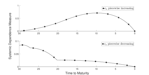
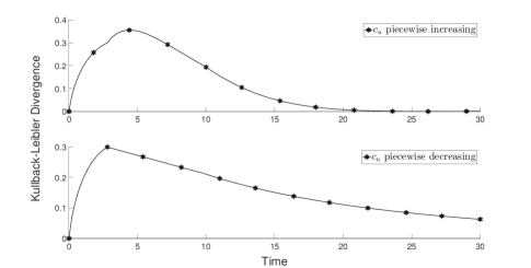
Refer to caption
(a) Systemic dependence measure
Refer to caption
(b) Kullback-Leibler divergence
Refer to caption
(c) Systemic instability measure
Figure 1: Systemic Dependence Measure, Kullback-Leibler Divergence, and Systemic Intability Measure for Example 5.1 (Contagious Common Jumps)

In the second part of the numerical analysis, we examine the systemic instability measure for two different dependence structures (5.25) and (5.31). In addition to the parameters in Table 2, we take parameter gu=ηmin(λu1,λu2)subscript𝑔𝑢𝜂superscriptsubscript𝜆𝑢1superscriptsubscript𝜆𝑢2g_{u}=\eta\min\left(\lambda_{u}^{1},\lambda_{u}^{2}\right) with η=0,0.5,0.8,1𝜂00.50.81\eta=0,0.5,0.8,1. If η=0𝜂0\eta=0, the structure (5.25) becomes the independence structure (5.19).

Refer to caption
Figure 2: Systemic Instability Measure for Example 5.1 (Contagious Common Jumps) with Piecewise Increasing cusubscript𝑐𝑢c_{u}
Refer to caption
Figure 3: Systemic Instability Measure for Example 5.1 (Contagious Common Jumps) with Piecewise Decreasing cusubscript𝑐𝑢c_{u}

In Figure 2 on page 2 and Figure 3 on page 3, we compare the systemic instability measure of the weak-only Markov structure to the strong Markov structures. It should be noted that when η=1𝜂1\eta=1, one of the components cannot jump individually. For instance, if min(λu1,λu2)=λu2superscriptsubscript𝜆𝑢1superscriptsubscript𝜆𝑢2superscriptsubscript𝜆𝑢2\min\left(\lambda_{u}^{1},\lambda_{u}^{2}\right)=\lambda_{u}^{2}, then the probability for X𝒮,2superscript𝑋𝒮2X^{\mathcal{S},2} jumping individually to state 111 is zero. In such a case, the level of systemic instability measure is highest. We argue that, since condition A is satisfied, the state of X𝒮,1superscript𝑋𝒮1X^{\mathcal{S},1} will not have an influence on how X𝒮,2superscript𝑋𝒮2X^{\mathcal{S},2} changes its state. However, if X𝒮,2superscript𝑋𝒮2X^{\mathcal{S},2} changes to state 111, X𝒮,1superscript𝑋𝒮1X^{\mathcal{S},1} must jump to state 111 as well. Financially speaking, the corresponding financial institution X𝒮,2superscript𝑋𝒮2X^{\mathcal{S},2} will not default individually. However, if X𝒮,2superscript𝑋𝒮2X^{\mathcal{S},2} defaults, then X𝒮,1superscript𝑋𝒮1X^{\mathcal{S},1} must default as well. The component X𝒮,2superscript𝑋𝒮2X^{\mathcal{S},2} contributes significantly to systemic risk.

After visualizing the basic behaviors of systemic instability measure, let us switch gears to more practical case: κ(1,1)(t+ΔT,t,2,X𝒟,(0,0))superscript𝜅11𝑡Δ𝑇𝑡2superscript𝑋𝒟00\kappa^{(1,1)}\left(t+\Delta T,t,2,X^{\mathcal{D}},(0,0)\right). As ΔTΔ𝑇\Delta T is fixed, the measure evaluates a fixed monitor period, from time t𝑡t to time t+ΔT𝑡Δ𝑇t+\Delta T, of the systemic condition at time t𝑡t. It will allow us to routinely monitor the future condition of the financial system, for instance, on the weekly basis. We consider two scenarios for the parameter cusubscript𝑐𝑢c_{u} fluctuating in different patterns. In the first scenario, cusubscript𝑐𝑢c_{u} starts with small value, then it becomes large and go down. The interpretation is that both financial institutions begins with good conditions. Then they deteriorate simultaneously through the common jumps factor, and become better again through the common jumps factor. Instead, the second scenario, cusubscript𝑐𝑢c_{u} will start with large value and cycle. We collect the parameters in Table 3.

Table 3: Parameters for Example 5.1 (Contagious Common Jumps): κ(1,1)(t+ΔT,t,2,X𝒟,(0,0))superscript𝜅11𝑡Δ𝑇𝑡2superscript𝑋𝒟00\kappa^{(1,1)}\left(t+\Delta T,t,2,X^{\mathcal{D}},(0,0)\right)
Parameters Time Periods
[0,6)06[0,6) [6,10)610[6,10) [10,20)1020[10,20) [20,26)2026[20,26) [26,30)2630[26,30) [30,)30[30,\infty)
a𝑎a 0.01 0.01 0.01 0.01 0.01 0.01
b𝑏b 0.02 0.02 0.02 0.02 0.02 0.02
Scenario 1: cusubscript𝑐𝑢c_{u} 0.01 0.09 0.03 0.12 0.04 0.04
Scenario 2: cusubscript𝑐𝑢c_{u} 0.12 0.09 0.03 0.09 0.05 0.05

In Figure 4 on page 4, all sequences of systemic instability measure fluctuate. As the monitor window ΔT=3Δ𝑇3\Delta T=3, the systemic instability measure uproars at t=3𝑡3t=3 reflecting the sudden change of cusubscript𝑐𝑢c_{u} in period [6,10)610[6,10). Analogously, the measure decreases at t=7𝑡7t=7 indicating the jump of cusubscript𝑐𝑢c_{u} in period [10,20)1020[10,20). Similar results can be observed in Figure 5 on page 5. We would like to emphasize that one Markov structure may behave more stable or unstable than other Markov structures throughout the entire tracking period.
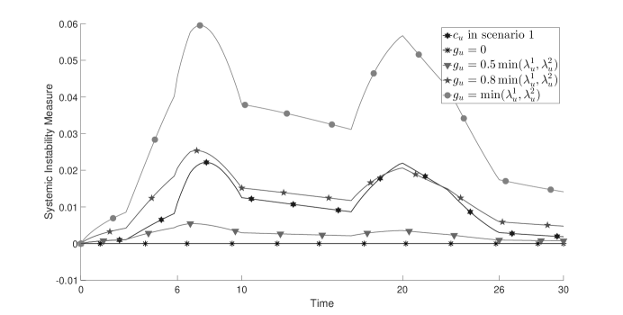
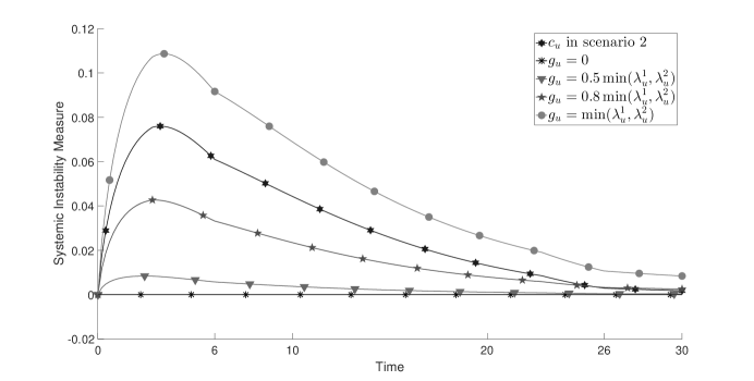
Refer to caption
Figure 4: Systemic Instability Measure for Example 5.1 (Contagious Common Jumps): Scenario 1
Refer to caption
Figure 5: Systemic Instability Measure for Example 5.1 (Contagious Common Jumps): Sceneario 2

Now, we use the same data in Table 3 while changing the lengths of monitor window ΔTΔ𝑇\Delta T, ΔT=0.6,1,3,5Δ𝑇0.6135\Delta T=0.6,1,3,5. The comparison is presented in Figure 6 on page 6. The sequence of systemic instability measure with shorter monitor window ΔTΔ𝑇\Delta T is embraced by the longer monitor window ΔTΔ𝑇\Delta T,

|κ(1,1)(t+ΔT1,t,2,X𝒟,(0,0))||κ(1,1)(t+ΔT2,t,2,X𝒟,(0,0))|,0ΔT1ΔT2<.formulae-sequencesuperscript𝜅11𝑡Δsubscript𝑇1𝑡2superscript𝑋𝒟00superscript𝜅11𝑡Δsubscript𝑇2𝑡2superscript𝑋𝒟000Δsubscript𝑇1Δsubscript𝑇2\left|\kappa^{(1,1)}\left(t+\Delta T_{1},t,2,X^{\mathcal{D}},(0,0)\right)\right|\leq\left|\kappa^{(1,1)}\left(t+\Delta T_{2},t,2,X^{\mathcal{D}},(0,0)\right)\right|,\quad 0\leq\Delta T_{1}\leq\Delta T_{2}<\infty.

From the perspective of risk management, this property should be expected as the uncertainty of a financial system for a longer period is generally higher.

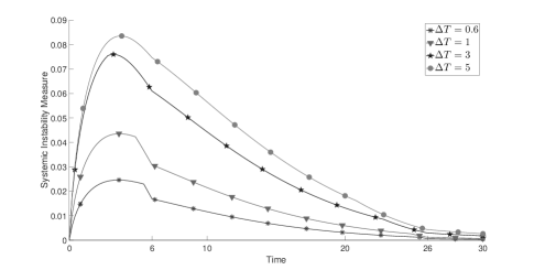
Refer to caption
(a) Scenario 1
Refer to caption
(b) Scenario 2
Figure 6: Systemic Instability Measure for Example 5.1 (Contagious Common Jumps) with Different Lengths of Monitor Window ΔTΔ𝑇\Delta T
Example 5.2 (Extreme contagion).

Assume that Yisuperscript𝑌𝑖Y^{i} is generated by ΛuisuperscriptsubscriptΛ𝑢𝑖\Lambda_{u}^{i},

ΛuisuperscriptsubscriptΛ𝑢𝑖\displaystyle\Lambda_{u}^{i} = (\@arstrut01\@arstrut0-cucu\@arstrut100) ,u0,i=1,2.formulae-sequenceabsent (\@arstrut01\@arstrut0-cucu\@arstrut100) formulae-sequence𝑢0𝑖12\displaystyle=\hbox{}\vbox{\kern 0.86108pt\hbox{$\kern 0.0pt\kern 2.5pt\kern-5.0pt\left(\kern 0.0pt\kern-2.5pt\kern-6.66669pt\vbox{\kern-0.86108pt\vbox{\vbox{ \halign{\kern\arraycolsep\hfil\@arstrut$\kbcolstyle#$\hfil\kern\arraycolsep& \kern\arraycolsep\hfil$\@kbrowstyle#$\ifkbalignright\relax\else\hfil\fi\kern\arraycolsep&& \kern\arraycolsep\hfil$\@kbrowstyle#$\ifkbalignright\relax\else\hfil\fi\kern\arraycolsep\cr 5.0pt\hfil\@arstrut$\scriptstyle$\hfil\kern 5.0pt&5.0pt\hfil$\scriptstyle 0$\hfil\kern 5.0pt&5.0pt\hfil$\scriptstyle 1$\hfil\kern 5.0pt\crcr\kern 0.86108pt\cr 5.0pt\hfil\@arstrut$\scriptstyle 0$\hfil\kern 5.0pt&5.0pt\hfil$-c_{u}$\hfil\kern 5.0pt&5.0pt\hfil$c_{u}$\hfil\kern 5.0pt\cr 5.0pt\hfil\@arstrut$\scriptstyle 1$\hfil\kern 5.0pt&5.0pt\hfil$0$\hfil\kern 5.0pt&5.0pt\hfil$0$\hfil\kern 5.0pt\cr}}}}\right)$}},\quad u\geq 0,\ i=1,2.

We solve for the solution (Λu𝒟,u0)superscriptsubscriptΛ𝑢𝒟𝑢0\left(\Lambda_{u}^{\mathcal{D}},u\geq 0\right) of the form,

Λu𝒟superscriptsubscriptΛ𝑢𝒟\displaystyle\Lambda_{u}^{\mathcal{D}} = (\@arstrut(0,0)(0,1)(1,0)(1,1) \@arstrut(0,0)-cu00cu\@arstrut(0,1)0000\@arstrut(1,0)0000\@arstrut(1,1)0000) ,absent (\@arstrut(0,0)(0,1)(1,0)(1,1) \@arstrut(0,0)-cu00cu\@arstrut(0,1)0000\@arstrut(1,0)0000\@arstrut(1,1)0000) \displaystyle=\hbox{}\vbox{\kern 0.86108pt\hbox{$\kern 0.0pt\kern 2.5pt\kern-5.0pt\left(\kern 0.0pt\kern-2.5pt\kern-6.66669pt\vbox{\kern-0.86108pt\vbox{\vbox{ \halign{\kern\arraycolsep\hfil\@arstrut$\kbcolstyle#$\hfil\kern\arraycolsep& \kern\arraycolsep\hfil$\@kbrowstyle#$\ifkbalignright\relax\else\hfil\fi\kern\arraycolsep&& \kern\arraycolsep\hfil$\@kbrowstyle#$\ifkbalignright\relax\else\hfil\fi\kern\arraycolsep\cr 5.0pt\hfil\@arstrut$\scriptstyle$\hfil\kern 5.0pt&5.0pt\hfil$\scriptstyle(0,0)$\hfil\kern 5.0pt&5.0pt\hfil$\scriptstyle(0,1)$\hfil\kern 5.0pt&5.0pt\hfil$\scriptstyle(1,0)$\hfil\kern 5.0pt&5.0pt\hfil$\scriptstyle(1,1)$\hfil\kern 5.0pt\crcr\kern 0.86108pt\cr 5.0pt\hfil\@arstrut$\scriptstyle(0,0)$\hfil\kern 5.0pt&5.0pt\hfil$-c_{u}$\hfil\kern 5.0pt&5.0pt\hfil$0$\hfil\kern 5.0pt&5.0pt\hfil$0$\hfil\kern 5.0pt&5.0pt\hfil$c_{u}$\hfil\kern 5.0pt\cr 5.0pt\hfil\@arstrut$\scriptstyle(0,1)$\hfil\kern 5.0pt&5.0pt\hfil$0$\hfil\kern 5.0pt&5.0pt\hfil$0$\hfil\kern 5.0pt&5.0pt\hfil$0$\hfil\kern 5.0pt&5.0pt\hfil$0$\hfil\kern 5.0pt\cr 5.0pt\hfil\@arstrut$\scriptstyle(1,0)$\hfil\kern 5.0pt&5.0pt\hfil$0$\hfil\kern 5.0pt&5.0pt\hfil$0$\hfil\kern 5.0pt&5.0pt\hfil$0$\hfil\kern 5.0pt&5.0pt\hfil$0$\hfil\kern 5.0pt\cr 5.0pt\hfil\@arstrut$\scriptstyle(1,1)$\hfil\kern 5.0pt&5.0pt\hfil$0$\hfil\kern 5.0pt&5.0pt\hfil$0$\hfil\kern 5.0pt&5.0pt\hfil$0$\hfil\kern 5.0pt&5.0pt\hfil$0$\hfil\kern 5.0pt\cr}}}}\right)$}}, (5.37)

where cu>0subscript𝑐𝑢0c_{u}>0 and piecewise constant. In view of (5.37), if the components jump, they must jump simultaneously. Note that in this structure, the transition probability for individual jump is zero. Hence, we call this structure as extreme contagion.

The parameters of this example are summarized in Table 4. We investigate the general properties of the systemic instability measure for the structure (5.37), and then compare the results to the structure (5.31) with different gusubscript𝑔𝑢g_{u}’s.

Table 4: Parameters for Example 5.2 (Extreme Contagion)
Parameters Time Periods
[0,6)06[0,6) [6,10)610[6,10) [10,20)1020[10,20) [20,26)2026[20,26) [26,30)2630[26,30) [30,)30[30,\infty)
Scenario 1: cusubscript𝑐𝑢c_{u} 0.010.010.01 0.10.10.1 0.080.080.08 0.050.050.05 0.030.030.03 0.030.030.03
Scenario 2: cusubscript𝑐𝑢c_{u} 0.080.080.08 0.030.030.03 0.020.020.02 0.040.040.04 0.030.030.03 0.030.030.03

In Figure 7 on page 7 and Figure 8 on page 8, an interesting observation is that the systemic instability measure of extreme contagion coincides with the measure obtained by gu=min(λu1,λu2)subscript𝑔𝑢superscriptsubscript𝜆𝑢1superscriptsubscript𝜆𝑢2g_{u}=\min\left(\lambda_{u}^{1},\lambda_{u}^{2}\right). The mathematical explanations are given below. First, Y1superscript𝑌1Y^{1} and Y2superscript𝑌2Y^{2} have the same law. For the structure (5.37), the chain does not move if it is not in state (0,0)00(0,0). For the structure (5.31), condition A is satisfied and the transition probability of individual jumps from state (0,0)00(0,0) is 00. Thus both structures produce the same levels of systemic instability.
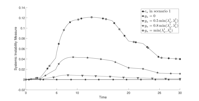
Refer to caption
Figure 7: Systemic Instability Measure for Example 5.2 (Extreme Contagion): Scenario 1
Refer to caption
Figure 8: Systemic Instability Measure for Example 5.2 (Extreme Contagion): Scenario 2
Example 5.3 (Extreme anti-contagion).

Consider Markov chains Y1,Y2superscript𝑌1superscript𝑌2Y^{1},Y^{2} with generators

ΛuisuperscriptsubscriptΛ𝑢𝑖\displaystyle\Lambda_{u}^{i} = (\@arstrut01\@arstrut0-λuiλui\@arstrut100) ,u0,i=1,2,formulae-sequenceabsent (\@arstrut01\@arstrut0-λuiλui\@arstrut100) formulae-sequence𝑢0𝑖12\displaystyle=\hbox{}\vbox{\kern 0.86108pt\hbox{$\kern 0.0pt\kern 2.5pt\kern-5.0pt\left(\kern 0.0pt\kern-2.5pt\kern-6.66669pt\vbox{\kern-0.86108pt\vbox{\vbox{ \halign{\kern\arraycolsep\hfil\@arstrut$\kbcolstyle#$\hfil\kern\arraycolsep& \kern\arraycolsep\hfil$\@kbrowstyle#$\ifkbalignright\relax\else\hfil\fi\kern\arraycolsep&& \kern\arraycolsep\hfil$\@kbrowstyle#$\ifkbalignright\relax\else\hfil\fi\kern\arraycolsep\cr 5.0pt\hfil\@arstrut$\scriptstyle$\hfil\kern 5.0pt&5.0pt\hfil$\scriptstyle 0$\hfil\kern 5.0pt&5.0pt\hfil$\scriptstyle 1$\hfil\kern 5.0pt\crcr\kern 0.86108pt\cr 5.0pt\hfil\@arstrut$\scriptstyle 0$\hfil\kern 5.0pt&5.0pt\hfil$-\lambda_{u}^{i}$\hfil\kern 5.0pt&5.0pt\hfil$\lambda_{u}^{i}$\hfil\kern 5.0pt\cr 5.0pt\hfil\@arstrut$\scriptstyle 1$\hfil\kern 5.0pt&5.0pt\hfil$0$\hfil\kern 5.0pt&5.0pt\hfil$0$\hfil\kern 5.0pt\cr}}}}\right)$}},\quad u\geq 0,\ i=1,2,

respectively, where

λu1=bu(au+bu)e0u(av+bv)dvau+bue0u(av+bv)dvλu2=au(au+bu)e0u(av+bv)dvbu+aue0u(av+bv)dv,superscriptsubscript𝜆𝑢1subscript𝑏𝑢subscript𝑎𝑢subscript𝑏𝑢superscriptesuperscriptsubscript0𝑢subscript𝑎𝑣subscript𝑏𝑣d𝑣subscript𝑎𝑢subscript𝑏𝑢superscriptesuperscriptsubscript0𝑢subscript𝑎𝑣subscript𝑏𝑣d𝑣superscriptsubscript𝜆𝑢2subscript𝑎𝑢subscript𝑎𝑢subscript𝑏𝑢superscriptesuperscriptsubscript0𝑢subscript𝑎𝑣subscript𝑏𝑣d𝑣subscript𝑏𝑢subscript𝑎𝑢superscriptesuperscriptsubscript0𝑢subscript𝑎𝑣subscript𝑏𝑣d𝑣\displaystyle\begin{split}\lambda_{u}^{1}&=\frac{b_{u}\left(a_{u}+b_{u}\right)\mathrm{e}^{-\int_{0}^{u}\left(a_{v}+b_{v}\right)\operatorname{d}\!v}}{a_{u}+b_{u}\mathrm{e}^{-\int_{0}^{u}\left(a_{v}+b_{v}\right)\operatorname{d}\!v}}\\ \lambda_{u}^{2}&=\frac{a_{u}\left(a_{u}+b_{u}\right)\mathrm{e}^{-\int_{0}^{u}\left(a_{v}+b_{v}\right)\operatorname{d}\!v}}{b_{u}+a_{u}\mathrm{e}^{-\int_{0}^{u}\left(a_{v}+b_{v}\right)\operatorname{d}\!v}},\end{split}

and au,bu>0subscript𝑎𝑢subscript𝑏𝑢0a_{u},b_{u}>0 and piecewise constant.

We solve for a Markov structure X𝒟superscript𝑋𝒟X^{\mathcal{D}} for {Y1,Y2}superscript𝑌1superscript𝑌2\left\{Y^{1},Y^{2}\right\} with generator (Λu𝒟,u0)superscriptsubscriptΛ𝑢𝒟𝑢0\left(\Lambda_{u}^{\mathcal{D}},u\geq 0\right) of the form,

Λu𝒟superscriptsubscriptΛ𝑢𝒟\displaystyle\Lambda_{u}^{\mathcal{D}} = (\@arstrut(0,0)(0,1)(1,0)(1,1)\@arstrut(0,0)-(au+bu)aubu0\@arstrut(0,1)0000\@arstrut(1,0)0000\@arstrut(1,1)0000) ,absent (\@arstrut(0,0)(0,1)(1,0)(1,1)\@arstrut(0,0)-(au+bu)aubu0\@arstrut(0,1)0000\@arstrut(1,0)0000\@arstrut(1,1)0000) \displaystyle=\hbox{}\vbox{\kern 0.86108pt\hbox{$\kern 0.0pt\kern 2.5pt\kern-5.0pt\left(\kern 0.0pt\kern-2.5pt\kern-6.66669pt\vbox{\kern-0.86108pt\vbox{\vbox{ \halign{\kern\arraycolsep\hfil\@arstrut$\kbcolstyle#$\hfil\kern\arraycolsep& \kern\arraycolsep\hfil$\@kbrowstyle#$\ifkbalignright\relax\else\hfil\fi\kern\arraycolsep&& \kern\arraycolsep\hfil$\@kbrowstyle#$\ifkbalignright\relax\else\hfil\fi\kern\arraycolsep\cr 5.0pt\hfil\@arstrut$\scriptstyle$\hfil\kern 5.0pt&5.0pt\hfil$\scriptstyle(0,0)$\hfil\kern 5.0pt&5.0pt\hfil$\scriptstyle(0,1)$\hfil\kern 5.0pt&5.0pt\hfil$\scriptstyle(1,0)$\hfil\kern 5.0pt&5.0pt\hfil$\scriptstyle(1,1)$\hfil\kern 5.0pt\crcr\kern 0.86108pt\cr 5.0pt\hfil\@arstrut$\scriptstyle(0,0)$\hfil\kern 5.0pt&5.0pt\hfil$-(a_{u}+b_{u})$\hfil\kern 5.0pt&5.0pt\hfil$a_{u}$\hfil\kern 5.0pt&5.0pt\hfil$b_{u}$\hfil\kern 5.0pt&5.0pt\hfil$0$\hfil\kern 5.0pt\cr 5.0pt\hfil\@arstrut$\scriptstyle(0,1)$\hfil\kern 5.0pt&5.0pt\hfil$0$\hfil\kern 5.0pt&5.0pt\hfil$0$\hfil\kern 5.0pt&5.0pt\hfil$0$\hfil\kern 5.0pt&5.0pt\hfil$0$\hfil\kern 5.0pt\cr 5.0pt\hfil\@arstrut$\scriptstyle(1,0)$\hfil\kern 5.0pt&5.0pt\hfil$0$\hfil\kern 5.0pt&5.0pt\hfil$0$\hfil\kern 5.0pt&5.0pt\hfil$0$\hfil\kern 5.0pt&5.0pt\hfil$0$\hfil\kern 5.0pt\cr 5.0pt\hfil\@arstrut$\scriptstyle(1,1)$\hfil\kern 5.0pt&5.0pt\hfil$0$\hfil\kern 5.0pt&5.0pt\hfil$0$\hfil\kern 5.0pt&5.0pt\hfil$0$\hfil\kern 5.0pt&5.0pt\hfil$0$\hfil\kern 5.0pt\cr}}}}\right)$}}, (5.43)

where au,bu>0subscript𝑎𝑢subscript𝑏𝑢0a_{u},b_{u}>0.

Unlike the structure (5.37) of extreme contagion, in view of the structure (5.43), every component jumps individually. It is impossible for both components to jump simultaneously,

(j=12𝟙{XT𝒟,j=1}2|Xt𝒟=(0,0))=0,t[0,T].\mathbb{P}\left(\sum_{j=1}^{2}\mathbbm{1}_{\left\{X_{T}^{\mathcal{D},j}=1\right\}}\geq 2\ \bigg{\rvert}\ X_{t}^{\mathcal{D}}=(0,0)\right)=0,\quad t\in[0,T]. (5.44)

We call this structure as extreme anti-contagion. The theoretical value of the systemic dependence measure is non-positive for any 0t<0𝑡0\leq t<\infty. The parameters for this example are given in Table 5.

Table 5: Parameters for Example 5.3 (Extreme Anti-contagion)
Parameters Time Periods
[0,6)06[0,6) [6,10)610[6,10) [10,20)1020[10,20) [20,26)2026[20,26) [26,30)2630[26,30) [30,)30[30,\infty)
Scenario 1: au=busubscript𝑎𝑢subscript𝑏𝑢a_{u}=b_{u} 0.010.010.01 0.080.080.08 0.050.050.05 0.030.030.03 0.010.010.01 0.010.010.01
Scenario 2: au=busubscript𝑎𝑢subscript𝑏𝑢a_{u}=b_{u} 0.050.050.05 0.020.020.02 0.030.030.03 0.070.070.07 0.050.050.05 0.050.050.05

In Figure 9 on page 9 and Figure 10 on page 10, every curve stands for the systemic instability measure as a function of t𝑡t. We observe that the systemic instability measures are indeed non-positive for the structure (5.43), and thus the financial system has favorable systemic dependence and is of systemic benefit. Besides, the financial system shares more favorable systemic benefit when the values of au,busubscript𝑎𝑢subscript𝑏𝑢a_{u},b_{u} get larger.

Refer to caption
Figure 9: Systemic Instability Measure for Example 5.3 (Extreme Anti-contagion): Scenario 1
Refer to caption
Figure 10: Systemic Instability Measure for Example 5.3 (Extreme Anti-contagion): Scenario 2
Example 5.4 (Systemic importance).

Consider Markov chains Y1,Y2superscript𝑌1superscript𝑌2Y^{1},Y^{2} with generators

ΛuisuperscriptsubscriptΛ𝑢𝑖\displaystyle\Lambda_{u}^{i} = (\@arstrut01\@arstrut0-λuiλui \@arstrut100) ,u0,i=1,2,formulae-sequenceabsent (\@arstrut01\@arstrut0-λuiλui \@arstrut100) formulae-sequence𝑢0𝑖12\displaystyle=\hbox{}\vbox{\kern 0.86108pt\hbox{$\kern 0.0pt\kern 2.5pt\kern-5.0pt\left(\kern 0.0pt\kern-2.5pt\kern-6.66669pt\vbox{\kern-0.86108pt\vbox{\vbox{ \halign{\kern\arraycolsep\hfil\@arstrut$\kbcolstyle#$\hfil\kern\arraycolsep& \kern\arraycolsep\hfil$\@kbrowstyle#$\ifkbalignright\relax\else\hfil\fi\kern\arraycolsep&& \kern\arraycolsep\hfil$\@kbrowstyle#$\ifkbalignright\relax\else\hfil\fi\kern\arraycolsep\cr 5.0pt\hfil\@arstrut$\scriptstyle$\hfil\kern 5.0pt&5.0pt\hfil$\scriptstyle 0$\hfil\kern 5.0pt&5.0pt\hfil$\scriptstyle 1$\hfil\kern 5.0pt\crcr\kern 0.86108pt\cr 5.0pt\hfil\@arstrut$\scriptstyle 0$\hfil\kern 5.0pt&5.0pt\hfil$-\lambda_{u}^{i}$\hfil\kern 5.0pt&5.0pt\hfil$\lambda_{u}^{i}$\hfil\kern 5.0pt\cr 5.0pt\hfil\@arstrut$\scriptstyle 1$\hfil\kern 5.0pt&5.0pt\hfil$0$\hfil\kern 5.0pt&5.0pt\hfil$0$\hfil\kern 5.0pt\cr}}}}\right)$}},\quad u\geq 0,\ i=1,2,

respectively, where

λu1=θu(cudu)+duλu2=au+cuθu=e0u(av+cv)dvcuduau+cudue0u(av+cv)dv+auau+cudue0udvdv,superscriptsubscript𝜆𝑢1subscript𝜃𝑢subscript𝑐𝑢subscript𝑑𝑢subscript𝑑𝑢superscriptsubscript𝜆𝑢2subscript𝑎𝑢subscript𝑐𝑢subscript𝜃𝑢superscriptesuperscriptsubscript0𝑢subscript𝑎𝑣subscript𝑐𝑣d𝑣subscript𝑐𝑢subscript𝑑𝑢subscript𝑎𝑢subscript𝑐𝑢subscript𝑑𝑢superscriptesuperscriptsubscript0𝑢subscript𝑎𝑣subscript𝑐𝑣d𝑣subscript𝑎𝑢subscript𝑎𝑢subscript𝑐𝑢subscript𝑑𝑢superscriptesuperscriptsubscript0𝑢subscript𝑑𝑣d𝑣\displaystyle\begin{split}\lambda_{u}^{1}&=\theta_{u}\left(c_{u}-d_{u}\right)+d_{u}\\ \lambda_{u}^{2}&=a_{u}+c_{u}\\ \theta_{u}&=\frac{\mathrm{e}^{-\int_{0}^{u}\left(a_{v}+c_{v}\right)\operatorname{d}\!v}}{\frac{c_{u}-d_{u}}{a_{u}+c_{u}-d_{u}}\mathrm{e}^{-\int_{0}^{u}\left(a_{v}+c_{v}\right)\operatorname{d}\!v}+\frac{a_{u}}{a_{u}+c_{u}-d_{u}}\mathrm{e}^{-\int_{0}^{u}d_{v}\operatorname{d}\!v}},\end{split}

with piecewise constant au,cu,du>0subscript𝑎𝑢subscript𝑐𝑢subscript𝑑𝑢0a_{u},c_{u},d_{u}>0, cudusubscript𝑐𝑢subscript𝑑𝑢c_{u}\neq d_{u}. Note that if cu=dusubscript𝑐𝑢subscript𝑑𝑢c_{u}=d_{u}, the generator in (5.50) is a strong Markov structure and coincides with the Λu𝒮superscriptsubscriptΛ𝑢𝒮\Lambda_{u}^{\mathcal{S}} with gu=min(λu1,λu2)subscript𝑔𝑢superscriptsubscript𝜆𝑢1superscriptsubscript𝜆𝑢2g_{u}=\min\left(\lambda_{u}^{1},\lambda_{u}^{2}\right).

It can be verified that a bivariate Markov chain X𝒟=(X𝒟,1,X𝒟,2)superscript𝑋𝒟superscript𝑋𝒟1superscript𝑋𝒟2X^{\mathcal{D}}=\left(X^{\mathcal{D},1},X^{\mathcal{D},2}\right) generated by (Λu𝒟,u0)superscriptsubscriptΛ𝑢𝒟𝑢0\left(\Lambda_{u}^{\mathcal{D}},u\geq 0\right),

Λu𝒟superscriptsubscriptΛ𝑢𝒟\displaystyle\Lambda_{u}^{\mathcal{D}} = (
\@arstrut (0,0) (0,1) (1,0) (1,1)
\@arstrut(0,0) -(+aucu) au 0 cu
\@arstrut(0,1) 0 -du 0 du
\@arstrut(1,0) 0 0 -(+aucu) +aucu
\@arstrut(1,1) 0 0 0 0
)
,
absent (
\@arstrut (0,0) (0,1) (1,0) (1,1)
\@arstrut(0,0) -(+aucu) au 0 cu
\@arstrut(0,1) 0 -du 0 du
\@arstrut(1,0) 0 0 -(+aucu) +aucu
\@arstrut(1,1) 0 0 0 0
)
\displaystyle=\hbox{}\vbox{\kern 0.86108pt\hbox{$\kern 0.0pt\kern 2.5pt\kern-5.0pt\left(\kern 0.0pt\kern-2.5pt\kern-6.66669pt\vbox{\kern-0.86108pt\vbox{\vbox{ \halign{\kern\arraycolsep\hfil\@arstrut$\kbcolstyle#$\hfil\kern\arraycolsep& \kern\arraycolsep\hfil$\@kbrowstyle#$\ifkbalignright\relax\else\hfil\fi\kern\arraycolsep&& \kern\arraycolsep\hfil$\@kbrowstyle#$\ifkbalignright\relax\else\hfil\fi\kern\arraycolsep\cr 5.0pt\hfil\@arstrut$\scriptstyle$\hfil\kern 5.0pt&5.0pt\hfil$\scriptstyle(0,0)$\hfil\kern 5.0pt&5.0pt\hfil$\scriptstyle(0,1)$\hfil\kern 5.0pt&5.0pt\hfil$\scriptstyle(1,0)$\hfil\kern 5.0pt&5.0pt\hfil$\scriptstyle(1,1)$\hfil\kern 5.0pt\crcr\kern 0.86108pt\cr 5.0pt\hfil\@arstrut$\scriptstyle(0,0)$\hfil\kern 5.0pt&5.0pt\hfil$-(a_{u}+c_{u})$\hfil\kern 5.0pt&5.0pt\hfil$a_{u}$\hfil\kern 5.0pt&5.0pt\hfil$0$\hfil\kern 5.0pt&5.0pt\hfil$c_{u}$\hfil\kern 5.0pt\cr 5.0pt\hfil\@arstrut$\scriptstyle(0,1)$\hfil\kern 5.0pt&5.0pt\hfil$0$\hfil\kern 5.0pt&5.0pt\hfil$-d_{u}$\hfil\kern 5.0pt&5.0pt\hfil$0$\hfil\kern 5.0pt&5.0pt\hfil$d_{u}$\hfil\kern 5.0pt\cr 5.0pt\hfil\@arstrut$\scriptstyle(1,0)$\hfil\kern 5.0pt&5.0pt\hfil$0$\hfil\kern 5.0pt&5.0pt\hfil$0$\hfil\kern 5.0pt&5.0pt\hfil$-(a_{u}+c_{u})$\hfil\kern 5.0pt&5.0pt\hfil$a_{u}+c_{u}$\hfil\kern 5.0pt\cr 5.0pt\hfil\@arstrut$\scriptstyle(1,1)$\hfil\kern 5.0pt&5.0pt\hfil$0$\hfil\kern 5.0pt&5.0pt\hfil$0$\hfil\kern 5.0pt&5.0pt\hfil$0$\hfil\kern 5.0pt&5.0pt\hfil$0$\hfil\kern 5.0pt\cr}}}}\right)$}},
(5.50)

is a weak Markov structure for {Y1,Y2}superscript𝑌1superscript𝑌2\left\{Y^{1},Y^{2}\right\}. Specifically, X𝒟,1superscript𝑋𝒟1X^{\mathcal{D},1} is Markovian in its own filtration, but not the filtration of X𝒟superscript𝑋𝒟X^{\mathcal{D}}. Whereas X𝒟,2superscript𝑋𝒟2X^{\mathcal{D},2} is Markovian in the filtration 𝔽Xsuperscript𝔽𝑋\mathbb{F}^{X}, and necessarily Markovian in its own filtration.

In view of (5.50), we know that

(Xs𝒟=(1,0)|Xt𝒟=(0,0))=0,0ts,formulae-sequencesuperscriptsubscript𝑋𝑠𝒟conditional10superscriptsubscript𝑋𝑡𝒟0000𝑡𝑠\mathbb{P}\left(X_{s}^{\mathcal{D}}=(1,0)\;|\;X_{t}^{\mathcal{D}}=(0,0)\right)=0,\quad 0\leq t\leq s,

and

0<(Xs𝒟,1=1|Xt𝒟=(0,0))(Xs𝒟,1=1|Xt𝒟=(0,1)),0ts.formulae-sequence0superscriptsubscript𝑋𝑠𝒟1conditional1superscriptsubscript𝑋𝑡𝒟00superscriptsubscript𝑋𝑠𝒟1conditional1superscriptsubscript𝑋𝑡𝒟010𝑡𝑠0<\mathbb{P}\left(X_{s}^{\mathcal{D},1}=1\;|\;X_{t}^{\mathcal{D}}=(0,0)\right)\neq\mathbb{P}\left(X_{s}^{\mathcal{D},1}=1\;|\;X_{t}^{\mathcal{D}}=(0,1)\right),\quad 0\leq t\leq s.

It means that X𝒟,1superscript𝑋𝒟1X^{\mathcal{D},1} cannot be in default alone. Saying differently, if X𝒟,1superscript𝑋𝒟1X^{\mathcal{D},1} defaults, X𝒟,2superscript𝑋𝒟2X^{\mathcal{D},2} must have defaulted at least earlier than X𝒟,1superscript𝑋𝒟1X^{\mathcal{D},1}. Moreover, it holds that

(Xs𝒟,2=1|Xt𝒟=(0,0))=(Xs𝒟,2=1|Xt𝒟=(1,0)),0ts.formulae-sequencesuperscriptsubscript𝑋𝑠𝒟2conditional1superscriptsubscript𝑋𝑡𝒟00superscriptsubscript𝑋𝑠𝒟2conditional1superscriptsubscript𝑋𝑡𝒟100𝑡𝑠\mathbb{P}\left(X_{s}^{\mathcal{D},2}=1\;|\;X_{t}^{\mathcal{D}}=(0,0)\right)=\mathbb{P}\left(X_{s}^{\mathcal{D},2}=1\;|\;X_{t}^{\mathcal{D}}=(1,0)\right),\quad 0\leq t\leq s.

Whether X𝒟,1superscript𝑋𝒟1X^{\mathcal{D},1} defaults or not, it does not impact on the default of X𝒟,2superscript𝑋𝒟2X^{\mathcal{D},2}. The relationship between X𝒟,1superscript𝑋𝒟1X^{\mathcal{D},1} and X𝒟,2superscript𝑋𝒟2X^{\mathcal{D},2} is similar to parasitism, and X𝒟,2superscript𝑋𝒟2X^{\mathcal{D},2} is the host. During a crisis, we would like to prevent X𝒟,2superscript𝑋𝒟2X^{\mathcal{D},2} from default to avoid Armageddon. Financially, we say that X𝒟,2superscript𝑋𝒟2X^{\mathcal{D},2} is systemically more important than X𝒟,1superscript𝑋𝒟1X^{\mathcal{D},1}. One remark should be made that this relationship between X𝒟,1superscript𝑋𝒟1X^{\mathcal{D},1} and X𝒟,2superscript𝑋𝒟2X^{\mathcal{D},2} is embedded in the structure of Λu𝒟superscriptsubscriptΛ𝑢𝒟\Lambda_{u}^{\mathcal{D}} given in (5.50). It is independent of functions a,c,d𝑎𝑐𝑑a,c,d.

Table 6: Parameters for Example 5.4 (Systemic Importance)
Parameters Time Periods
[0,6)06[0,6) [6,10)610[6,10) [10,20)1020[10,20) [20,26)2026[20,26) [26,30)2630[26,30) [30,)30[30,\infty)
Scenario 1: ausubscript𝑎𝑢a_{u} 0.02 0.02 0.02 0.02 0.02 0.02
cusubscript𝑐𝑢c_{u} 0.02 0.09 0.06 0.02 0.09 0.09
dusubscript𝑑𝑢d_{u} 0.01 0.01 0.01 0.01 0.01 0.01
Scenario 2: ausubscript𝑎𝑢a_{u} 0.02 0.02 0.02 0.02 0.02 0.02
cusubscript𝑐𝑢c_{u} 0.09 0.06 0.02 0.09 0.02 0.02
dusubscript𝑑𝑢d_{u} 0.01 0.01 0.01 0.01 0.01 0.01

Now, we turn our attention to the numerical results. In what follows, we would like to study the effect of the second distress. The parameters are provided in Table 6. Both scenarios have the same parameters in ausubscript𝑎𝑢a_{u} and dusubscript𝑑𝑢d_{u}, but different cusubscript𝑐𝑢c_{u} cycling. In scenario 1, the simulated system embarks from good condition, in the sense of the magnitude of cusubscript𝑐𝑢c_{u}, while in scenario 2 the simulated system starts from bad condition. In Figure 11 on page 11 and Figure 12 on page 12, X𝒟superscript𝑋𝒟X^{\mathcal{D}} produces the highest level in systemic instability in both scenarios. This unsymmetrical relationship between two components is considered more risky than the other dependence structures, which allow individual default symmetrically. Next observation is regarding the second distress occurred in period [26,30)2630[26,30) of scenario 1 and in period [20,26)2026[20,26) of scenario 2. Although the impact of the second distress is inconclusive555We may have higher systemic instability in the second distress with different time periods setting. For instance, see Figure 13 on page 13 by using the same parameters of scenario 1 in Table 6 with time periods [0,6)06[0,6), [6,8)68[6,8), [8,10)810[8,10), [10,12)1012[10,12), [12,15)1215[12,15), [15,)15[15,\infty)., the systemic instability in scenario 2 is indeed higher if the system starts from the bad condition.
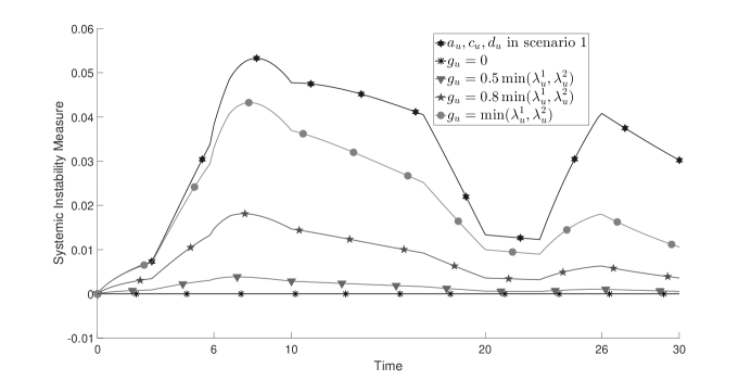
Refer to caption
Figure 11: Systemic Instability Measure for Example 5.4 (Systemic Importance): Scenario 1
Refer to caption
Figure 12: Systemic Instability Measure for Example 5.4 (Systemic Importance): Scenario 2
Refer to caption
Figure 13: Systemic Instability Measure for Example 5.4 (Systemic Importance): Scenario 1 with Time Periods [0,6),[6,8),[8,10),[10,12),[12,15),[15,)06688101012121515[0,6),[6,8),[8,10),[10,12),[12,15),[15,\infty).
Example 5.5 (Two weak-only Markov strcutures).

In this final example, we will compare systemic instability measures of two weak-only Markov structures for the same collection of identical Markov chains {Y1,Y2}superscript𝑌1superscript𝑌2\{Y^{1},Y^{2}\}. Specifically, we take a=b𝑎𝑏a=b in (5.13) and obtain λu1=λu2superscriptsubscript𝜆𝑢1superscriptsubscript𝜆𝑢2\lambda_{u}^{1}=\lambda_{u}^{2}. We use this simple example to show that a financial system with distinct dependence structures produces different levels of systemic instability. In addition, the results are consistent with financial intuitions.

The first weak-only Markov structure (Λu𝒟,u0)superscriptsubscriptΛ𝑢𝒟𝑢0\left(\Lambda_{u}^{\mathcal{D}},u\geq 0\right) is of the form

Λu𝒟superscriptsubscriptΛ𝑢𝒟\displaystyle\Lambda_{u}^{\mathcal{D}} = (\@arstrut(0,0)(0,1)(1,0)(1,1)\@arstrut(0,0)-(2a+cu)aacu\@arstrut(0,1)0-a0a\@arstrut(1,0)00-aa\@arstrut(1,1)0000) ,absent (\@arstrut(0,0)(0,1)(1,0)(1,1)\@arstrut(0,0)-(2a+cu)aacu\@arstrut(0,1)0-a0a\@arstrut(1,0)00-aa\@arstrut(1,1)0000) \displaystyle=\hbox{}\vbox{\kern 0.86108pt\hbox{$\kern 0.0pt\kern 2.5pt\kern-5.0pt\left(\kern 0.0pt\kern-2.5pt\kern-6.66669pt\vbox{\kern-0.86108pt\vbox{\vbox{ \halign{\kern\arraycolsep\hfil\@arstrut$\kbcolstyle#$\hfil\kern\arraycolsep& \kern\arraycolsep\hfil$\@kbrowstyle#$\ifkbalignright\relax\else\hfil\fi\kern\arraycolsep&& \kern\arraycolsep\hfil$\@kbrowstyle#$\ifkbalignright\relax\else\hfil\fi\kern\arraycolsep\cr 5.0pt\hfil\@arstrut$\scriptstyle$\hfil\kern 5.0pt&5.0pt\hfil$\scriptstyle(0,0)$\hfil\kern 5.0pt&5.0pt\hfil$\scriptstyle(0,1)$\hfil\kern 5.0pt&5.0pt\hfil$\scriptstyle(1,0)$\hfil\kern 5.0pt&5.0pt\hfil$\scriptstyle(1,1)$\hfil\kern 5.0pt\crcr\kern 0.86108pt\cr 5.0pt\hfil\@arstrut$\scriptstyle(0,0)$\hfil\kern 5.0pt&5.0pt\hfil$-(2a+c_{u})$\hfil\kern 5.0pt&5.0pt\hfil$a$\hfil\kern 5.0pt&5.0pt\hfil$a$\hfil\kern 5.0pt&5.0pt\hfil$c_{u}$\hfil\kern 5.0pt\cr 5.0pt\hfil\@arstrut$\scriptstyle(0,1)$\hfil\kern 5.0pt&5.0pt\hfil$0$\hfil\kern 5.0pt&5.0pt\hfil$-a$\hfil\kern 5.0pt&5.0pt\hfil$0$\hfil\kern 5.0pt&5.0pt\hfil$a$\hfil\kern 5.0pt\cr 5.0pt\hfil\@arstrut$\scriptstyle(1,0)$\hfil\kern 5.0pt&5.0pt\hfil$0$\hfil\kern 5.0pt&5.0pt\hfil$0$\hfil\kern 5.0pt&5.0pt\hfil$-a$\hfil\kern 5.0pt&5.0pt\hfil$a$\hfil\kern 5.0pt\cr 5.0pt\hfil\@arstrut$\scriptstyle(1,1)$\hfil\kern 5.0pt&5.0pt\hfil$0$\hfil\kern 5.0pt&5.0pt\hfil$0$\hfil\kern 5.0pt&5.0pt\hfil$0$\hfil\kern 5.0pt&5.0pt\hfil$0$\hfil\kern 5.0pt\cr}}}}\right)$}}, (5.56)

and the second weak-only Markov structure comes from Example 5.2 with (Λu𝒟,u0)superscriptsubscriptΛ𝑢𝒟𝑢0\left(\Lambda_{u}^{\mathcal{D}},u\geq 0\right) of the form

Λu𝒟superscriptsubscriptΛ𝑢𝒟\displaystyle\Lambda_{u}^{\mathcal{D}} = (
\@arstrut (0,0) (0,1) (1,0) (1,1)
\@arstrut(0,0) -λu1 0 0 λu1
\@arstrut(0,1) 0 0 0 0
\@arstrut(1,0) 0 0 0 0
\@arstrut(1,1) 0 0 0 0
)
.
absent (
\@arstrut (0,0) (0,1) (1,0) (1,1)
\@arstrut(0,0) -λu1 0 0 λu1
\@arstrut(0,1) 0 0 0 0
\@arstrut(1,0) 0 0 0 0
\@arstrut(1,1) 0 0 0 0
)
\displaystyle=\hbox{}\vbox{\kern 0.86108pt\hbox{$\kern 0.0pt\kern 2.5pt\kern-5.0pt\left(\kern 0.0pt\kern-2.5pt\kern-6.66669pt\vbox{\kern-0.86108pt\vbox{\vbox{ \halign{\kern\arraycolsep\hfil\@arstrut$\kbcolstyle#$\hfil\kern\arraycolsep& \kern\arraycolsep\hfil$\@kbrowstyle#$\ifkbalignright\relax\else\hfil\fi\kern\arraycolsep&& \kern\arraycolsep\hfil$\@kbrowstyle#$\ifkbalignright\relax\else\hfil\fi\kern\arraycolsep\cr 5.0pt\hfil\@arstrut$\scriptstyle$\hfil\kern 5.0pt&5.0pt\hfil$\scriptstyle(0,0)$\hfil\kern 5.0pt&5.0pt\hfil$\scriptstyle(0,1)$\hfil\kern 5.0pt&5.0pt\hfil$\scriptstyle(1,0)$\hfil\kern 5.0pt&5.0pt\hfil$\scriptstyle(1,1)$\hfil\kern 5.0pt\crcr\kern 0.86108pt\cr 5.0pt\hfil\@arstrut$\scriptstyle(0,0)$\hfil\kern 5.0pt&5.0pt\hfil$-\lambda_{u}^{1}$\hfil\kern 5.0pt&5.0pt\hfil$0$\hfil\kern 5.0pt&5.0pt\hfil$0$\hfil\kern 5.0pt&5.0pt\hfil$\lambda_{u}^{1}$\hfil\kern 5.0pt\cr 5.0pt\hfil\@arstrut$\scriptstyle(0,1)$\hfil\kern 5.0pt&5.0pt\hfil$0$\hfil\kern 5.0pt&5.0pt\hfil$0$\hfil\kern 5.0pt&5.0pt\hfil$0$\hfil\kern 5.0pt&5.0pt\hfil$0$\hfil\kern 5.0pt\cr 5.0pt\hfil\@arstrut$\scriptstyle(1,0)$\hfil\kern 5.0pt&5.0pt\hfil$0$\hfil\kern 5.0pt&5.0pt\hfil$0$\hfil\kern 5.0pt&5.0pt\hfil$0$\hfil\kern 5.0pt&5.0pt\hfil$0$\hfil\kern 5.0pt\cr 5.0pt\hfil\@arstrut$\scriptstyle(1,1)$\hfil\kern 5.0pt&5.0pt\hfil$0$\hfil\kern 5.0pt&5.0pt\hfil$0$\hfil\kern 5.0pt&5.0pt\hfil$0$\hfil\kern 5.0pt&5.0pt\hfil$0$\hfil\kern 5.0pt\cr}}}}\right)$}}.
(5.62)

Both Markov structures (5.56) and (5.62) are the solutions of

Λui=ΘuiΛu𝒟Φi,u0,i=1,2,formulae-sequencesuperscriptsubscriptΛ𝑢𝑖superscriptsubscriptΘ𝑢𝑖superscriptsubscriptΛ𝑢𝒟superscriptΦ𝑖formulae-sequence𝑢0𝑖12\Lambda_{u}^{i}=\Theta_{u}^{i}\Lambda_{u}^{\mathcal{D}}\Phi^{i},\quad u\geq 0,\ i=1,2,

with Λu1=Λu2superscriptsubscriptΛ𝑢1superscriptsubscriptΛ𝑢2\Lambda_{u}^{1}=\Lambda_{u}^{2}.

The parameters are listed in Table 7 on page 7. In Figure 14 on page 14, we observe that the X𝒟superscript𝑋𝒟X^{\mathcal{D}} with extreme contagious structure produces higher values in systemic instability measure in both scenarios. This result is consistent with financial intuitions. If two financial institutions only default simultaneously, as we are measuring the event of Armageddon, this financial system is certainly more unstable than allowing any financial institution to default individually. Because the financial system allowing single default will be relatively away from Armageddon. Moreover, the system beginning with bad condition, i.e. scenario 2, generally behaves more unstable.

Table 7: Parameters for Example 5.5 (Two Weak-only Markov Structures)
Parameters Time Periods
[0,6)06[0,6) [6,10)610[6,10) [10,20)1020[10,20) [20,26)2026[20,26) [26,30)2630[26,30) [30,)30[30,\infty)
a=b𝑎𝑏a=b 0.01 0.01 0.01 0.01 0.01 0.01
Scenario 1: cusubscript𝑐𝑢c_{u} 0.02 0.09 0.06 0.02 0.09 0.09
Scenario 2: cusubscript𝑐𝑢c_{u} 0.09 0.06 0.02 0.09 0.02 0.02
Refer to caption
(a) Scenario 1
Refer to caption
(b) Scenario 2
Figure 14: Systemic Instability Measure for Example 5.5 (Two Weak-only Markov Structures)

Appendix A Technical Results

In this section, we borrow condition A from [8] and collect relevant results from [13] to lay the basis for our work. Recall the setting in Section 2, let X=(X1,,Xm)𝑋superscript𝑋1superscript𝑋𝑚X=\left(X^{1},\ldots,X^{m}\right) be a multivariate Markov chain and take values in E=E1××Em𝐸subscript𝐸1subscript𝐸𝑚E=E_{1}\times\cdots\times E_{m}. First, we state several conditions.

Condition (M). We say the generator matrix function ΛtsubscriptΛ𝑡\Lambda_{t} satisfies condition (M) if ΛtsubscriptΛ𝑡\Lambda_{t} satisfies for every t0𝑡0t\geq 0, i=1,2,,m𝑖12𝑚i=1,2,\ldots,m,

(𝐌i)y(yi)λtx,y=y(yi)λtx^,y,xj,x^j,yjEj,j=1,2,,m,x,x^(xi),xiyi.formulae-sequence𝐌𝑖subscript𝑦superscript𝑦𝑖superscriptsubscript𝜆𝑡𝑥𝑦subscript𝑦superscript𝑦𝑖superscriptsubscript𝜆𝑡^𝑥𝑦superscript𝑥𝑗superscript^𝑥𝑗superscript𝑦𝑗subscript𝐸𝑗formulae-sequence𝑗12𝑚𝑥formulae-sequence^𝑥superscript𝑥𝑖superscript𝑥𝑖superscript𝑦𝑖\left(\mathbf{M}\mathit{i}\right)\quad\sum_{y\in\mathcal{H}\left(y^{i}\right)}\lambda_{t}^{x,y}=\sum_{y\in\mathcal{H}\left(y^{i}\right)}\lambda_{t}^{\hat{x},y},\quad x^{j},\hat{x}^{j},y^{j}\in E_{j},\ j=1,2,\ldots,m,\ x,\hat{x}\in\mathcal{H}\left(x^{i}\right),\ x^{i}\neq y^{i}.

Specifically,

x=(x1,,xi,,xm),x^=(x^1,,xi,,x^m),y=(y1,,yi,,ym).formulae-sequence𝑥superscript𝑥1superscript𝑥𝑖superscript𝑥𝑚formulae-sequence^𝑥superscript^𝑥1superscript𝑥𝑖superscript^𝑥𝑚𝑦superscript𝑦1superscript𝑦𝑖superscript𝑦𝑚x=\left(x^{1},\ldots,x^{i},\ldots,x^{m}\right),\ \hat{x}=\left(\hat{x}^{1},\ldots,x^{i},\ldots,\hat{x}^{m}\right),\ y=\left(y^{1},\ldots,y^{i},\ldots,y^{m}\right).

Condition (P). We say the transition probability function 𝐏t,ssubscript𝐏𝑡𝑠\mathbf{P}_{t,s} satisfies condition (P) if for any 0ts<0𝑡𝑠0\leq t\leq s<\infty, i=1,2,,m𝑖12𝑚i=1,2,\ldots,m, we have

(𝐏i)y(yi)𝐏t,sx,y=y(yi)𝐏t,sx^,y,xj,x^j,yjEj,j=1,2,,m,x,x^(xi),xiyi.formulae-sequence𝐏𝑖subscript𝑦superscript𝑦𝑖superscriptsubscript𝐏𝑡𝑠𝑥𝑦subscript𝑦superscript𝑦𝑖superscriptsubscript𝐏𝑡𝑠^𝑥𝑦superscript𝑥𝑗superscript^𝑥𝑗superscript𝑦𝑗subscript𝐸𝑗formulae-sequence𝑗12𝑚𝑥formulae-sequence^𝑥superscript𝑥𝑖superscript𝑥𝑖superscript𝑦𝑖\left(\mathbf{P}\mathit{i}\right)\quad\sum_{y\in\mathcal{H}\left(y^{i}\right)}\mathbf{P}_{t,s}^{x,y}=\sum_{y\in\mathcal{H}\left(y^{i}\right)}\mathbf{P}_{t,s}^{\hat{x},y},\quad x^{j},\hat{x}^{j},y^{j}\in E_{j},\ j=1,2,\ldots,m,\ x,\hat{x}\in\mathcal{H}\left(x^{i}\right),\ x^{i}\neq y^{i}.

It was proved in [13, Proposition A.2] that condition A is equivalent to condition A.

Theorem A.1.

Assume that

(Xt=z)>0,dta.e.,zE.\mathbb{P}\left(X_{t}=z\right)>0,\ dt\operatorname{-a.e.},\quad z\in E. (A.1)

Then strong Markovian consistency implies condition A.

We denote by ΠtsubscriptΠ𝑡\Pi_{t} the collection of all finite partitions of interval [0,t]0𝑡[0,t], namely,

Πt={πt={0,t1,,tn1,t}| 0=t0<t1<<tn=t,n}.subscriptΠ𝑡conditional-setsubscript𝜋𝑡0subscript𝑡1subscript𝑡𝑛1𝑡formulae-sequence 0subscript𝑡0subscript𝑡1subscript𝑡𝑛𝑡𝑛\Pi_{t}=\left\{\pi_{t}=\{0,t_{1},\ldots,t_{n-1},t\}\;|\;0=t_{0}<t_{1}<\cdots<t_{n}=t,\ n\in\mathbb{N}\right\}.

We denote by Einsuperscriptsubscript𝐸𝑖𝑛E_{i}^{n} the n𝑛n-fold Cartesian product of Eisubscript𝐸𝑖E_{i}. Let ψ(a)𝜓𝑎\psi(a) be a vector in Ein+1superscriptsubscript𝐸𝑖𝑛1E_{i}^{n+1} with the last element in a𝑎a. Moreover, ΥisuperscriptΥ𝑖\Upsilon^{i} denotes the projection operator acting on the initial distribution,

(ΥiμX)(Γ)=(X0iΓi),ΓE,ΓiEi.formulae-sequencesuperscriptΥ𝑖superscript𝜇𝑋Γsuperscriptsubscript𝑋0𝑖superscriptΓ𝑖formulae-sequenceΓ𝐸superscriptΓ𝑖subscript𝐸𝑖\left(\Upsilon^{i}\mu^{X}\right)\left(\Gamma\right)=\mathbb{P}\left(X_{0}^{i}\in\Gamma^{i}\right),\quad\Gamma\subset E,\ \Gamma^{i}\subset E_{i}.
Theorem A.2.

The component Xisuperscript𝑋𝑖X^{i} of X𝑋X is a Markov chain in its natural filtration if and only if for 0ts0𝑡𝑠0\leq t\leq s, any xti,xsiEisuperscriptsubscript𝑥𝑡𝑖superscriptsubscript𝑥𝑠𝑖subscript𝐸𝑖x_{t}^{i},x_{s}^{i}\in E_{i}, ψ(xti)Ein+1𝜓superscriptsubscript𝑥𝑡𝑖superscriptsubscript𝐸𝑖𝑛1\psi(x_{t}^{i})\in E_{i}^{n+1}, any πtΠtsubscript𝜋𝑡subscriptΠ𝑡\pi_{t}\in\Pi_{t}, the following holds,

xt(xti)Ξi(t,xt,ψ(xti),πt,μX)𝐏t,sxt,xsi=0,subscriptsubscript𝑥𝑡superscriptsubscript𝑥𝑡𝑖superscriptΞ𝑖𝑡subscript𝑥𝑡𝜓superscriptsubscript𝑥𝑡𝑖subscript𝜋𝑡superscript𝜇𝑋superscriptsubscript𝐏𝑡𝑠subscript𝑥𝑡superscriptsubscript𝑥𝑠𝑖0\sum_{x_{t}\in\mathcal{H}\left(x_{t}^{i}\right)}\Xi^{i}\left(t,x_{t},\psi(x_{t}^{i}),\pi_{t},\mu^{X}\right)\mathbf{P}_{t,s}^{x_{t},x_{s}^{i}}=0, (A.2)

where

Ξi(t,xt,ψ(xti),πt,μX)superscriptΞ𝑖𝑡subscript𝑥𝑡𝜓superscriptsubscript𝑥𝑡𝑖subscript𝜋𝑡superscript𝜇𝑋\displaystyle\Xi^{i}\left(t,x_{t},\psi(x_{t}^{i}),\pi_{t},\mu^{X}\right) :=(Xt=xt|Xti=xti,Xtn1i=xn1i,,X0i=x0i)(Xt=xt|Xti=xti)\displaystyle:=\mathbb{P}\left(X_{t}=x_{t}\;|\;X_{t}^{i}=x_{t}^{i},\ X_{t_{n-1}}^{i}=x_{n-1}^{i},\ldots,\ X_{0}^{i}=x_{0}^{i}\right)-\mathbb{P}\left(X_{t}=x_{t}\;|\;X_{t}^{i}=x_{t}^{i}\right)
𝐏t,sxt,xsisuperscriptsubscript𝐏𝑡𝑠subscript𝑥𝑡superscriptsubscript𝑥𝑠𝑖\displaystyle\mathbf{P}_{t,s}^{x_{t},x_{s}^{i}} :=(Xsi=xsi|Xt=xt).assignabsentsuperscriptsubscript𝑋𝑠𝑖conditionalsuperscriptsubscript𝑥𝑠𝑖subscript𝑋𝑡subscript𝑥𝑡\displaystyle:=\mathbb{P}\left(X_{s}^{i}=x_{s}^{i}\;|\;X_{t}=x_{t}\right).

We state the condition A.

Condition (Ci𝑖i). Given μX>0superscript𝜇𝑋0\mu^{X}>0, for any t0𝑡0t\geq 0, xtiEi,xt(xti),ψ(xti)Ein+1formulae-sequencesuperscriptsubscript𝑥𝑡𝑖subscript𝐸𝑖formulae-sequencesubscript𝑥𝑡superscriptsubscript𝑥𝑡𝑖𝜓superscriptsubscript𝑥𝑡𝑖superscriptsubscript𝐸𝑖𝑛1x_{t}^{i}\in E_{i},\ x_{t}\in\mathcal{H}\left(x_{t}^{i}\right),\ \psi(x_{t}^{i})\in E_{i}^{n+1}, and πtΠtsubscript𝜋𝑡subscriptΠ𝑡\pi_{t}\in\Pi_{t},

Ξi(t,xt,ψ(xti),πt,μX)=0.superscriptΞ𝑖𝑡subscript𝑥𝑡𝜓superscriptsubscript𝑥𝑡𝑖subscript𝜋𝑡superscript𝜇𝑋0\Xi^{i}\left(t,x_{t},\psi(x_{t}^{i}),\pi_{t},\mu^{X}\right)=0.
Theorem A.3.

Assume that a multivariate Markov chain X=(X1,,Xm)𝑋superscript𝑋1superscript𝑋𝑚X=\left(X^{1},\ldots,X^{m}\right) has infinitesimal generator (Λu,u0)subscriptΛ𝑢𝑢0\left(\Lambda_{u},u\geq 0\right) with transition semigroup (𝐏t,s,0ts)subscript𝐏𝑡𝑠0𝑡𝑠\left(\mathbf{P}_{t,s},0\leq t\leq s\right). If there exists an initial distribution μX>0superscript𝜇𝑋0\mu^{X}>0 such that the transition semigroup 𝐏^t,sisuperscriptsubscript^𝐏𝑡𝑠𝑖\widehat{\mathbf{P}}_{t,s}^{i} of (ΘuiΛuΦi,u0)superscriptsubscriptΘ𝑢𝑖subscriptΛ𝑢superscriptΦ𝑖𝑢0\left(\Theta_{u}^{i}\Lambda_{u}\Phi^{i},u\geq 0\right) satisfies the identity

Θti𝐏t,s=𝐏^t,siΘsi,0ts,formulae-sequencesuperscriptsubscriptΘ𝑡𝑖subscript𝐏𝑡𝑠superscriptsubscript^𝐏𝑡𝑠𝑖superscriptsubscriptΘ𝑠𝑖0𝑡𝑠\Theta_{t}^{i}\mathbf{P}_{t,s}=\widehat{\mathbf{P}}_{t,s}^{i}\Theta_{s}^{i},\quad 0\leq t\leq s, (A.3)

then

  1. (i)

    𝐏t,si=𝐏^t,sisuperscriptsubscript𝐏𝑡𝑠𝑖superscriptsubscript^𝐏𝑡𝑠𝑖\mathbf{P}_{t,s}^{i}=\widehat{\mathbf{P}}_{t,s}^{i}, where 𝐏t,sisuperscriptsubscript𝐏𝑡𝑠𝑖\mathbf{P}_{t,s}^{i} is the semigroup of Xisuperscript𝑋𝑖X^{i};

  2. (ii)

    condition A holds true.

Corollary A.4.

If the assumptions in Theorem A.3 hold true, then the component Xisuperscript𝑋𝑖X^{i} of X𝑋X is Markov in its natural filtration with the initial distribution ΥiμXsuperscriptΥ𝑖superscript𝜇𝑋\Upsilon^{i}\mu^{X}. Moreover, Xisuperscript𝑋𝑖X^{i} has the generator (ΘtiΛtΦi,t0)superscriptsubscriptΘ𝑡𝑖subscriptΛ𝑡superscriptΦ𝑖𝑡0\left(\Theta_{t}^{i}\Lambda_{t}\Phi^{i},t\geq 0\right).

We conclude this section by presenting the conditions for X𝑋X to be weak-only Markovian consistent with respect to the component Xisuperscript𝑋𝑖X^{i}.

Theorem A.5.

Suppose that X𝑋X is a multivariate Markov chain generated by (Λt,t0)subscriptΛ𝑡𝑡0\left(\Lambda_{t},t\geq 0\right) with initial distribution μX>0superscript𝜇𝑋0\mu^{X}>0. If the following conditions are satisfied,

  1. (i)

    for any 0ts0𝑡𝑠0\leq t\leq s, xti,xsiEisuperscriptsubscript𝑥𝑡𝑖superscriptsubscript𝑥𝑠𝑖subscript𝐸𝑖x_{t}^{i},x_{s}^{i}\in E_{i}, ψ(xti)Ein+1𝜓superscriptsubscript𝑥𝑡𝑖superscriptsubscript𝐸𝑖𝑛1\psi\left(x_{t}^{i}\right)\in E_{i}^{n+1}, and πtΠtsubscript𝜋𝑡subscriptΠ𝑡\pi_{t}\in\Pi_{t}, Equation (A.2) holds true;

  2. (ii)

    the inequality holds,

    (Xt=x)>0,dta.e.,xE;\mathbb{P}\left(X_{t}=x\right)>0,\ dt\operatorname{-a.e.},\quad x\in E;
  3. (iii)

    condition A (or equivalently, condition A) does not hold,

then the component Xisuperscript𝑋𝑖X^{i} of X𝑋X is a Markov chain in its natural filtration, but not a Markov chain in the filtration of X𝑋X. Necessarily, the initial distribution of Xisuperscript𝑋𝑖X^{i} is ΥiμXsuperscriptΥ𝑖superscript𝜇𝑋\Upsilon^{i}\mu^{X} and the generator of Xisuperscript𝑋𝑖X^{i} coincides with (ΘtiΛtΦi,t0)superscriptsubscriptΘ𝑡𝑖subscriptΛ𝑡superscriptΦ𝑖𝑡0\left(\Theta_{t}^{i}\Lambda_{t}\Phi^{i},t\geq 0\right).

Acknowledgments

The author greatly thanks Prof. Tomasz R. Bielecki and Prof. Igor Cialenco for their enlightening comments and helpful discussions.

References

  • AM [12] H. Amini and A. Minca. Mathematical modeling of systemic risk. In Advances in network analysis and its applications, pages 3–26. Springer, 2012.
  • APPR [12] V. V. Acharya, L. H. Pedersen, T. Philippon, and M. P. Richardson. Measuring systemic risk. London, Centre for Economic Policy Research, 2012.
  • BC [15] L. Bo and A. Capponi. Systemic risk in interbanking networks. SIAM Journal on Financial Mathematics, 6(1):386–424, 2015.
  • BCCH [14] T. R. Bielecki, A. Cousin, S. Crépey, and A. Herbertsson. Dynamic hedging of portfolio credit risk in a Markov copula model. J. Optim. Theory Appl., 161(1):90–102, 2014.
  • BCF [18] T. R. Bielecki, I. Cialenco, and S. Feng. A dynamic model of central counterparty risk. 2018. arXiv:1803.02012v1.
  • BFFMB [15] F. Biagini, J.-P. Fouque, M. Frittelli, and T. Meyer-Brandis. A unified approach to systemic risk measures via acceptance sets. arXiv preprint arXiv:1503.06354, 2015.
  • BFLV [12] D. Bisias, M. Flood, A. W. Lo, and S. Valavanis. A survey of systemic risk analytics. Annual Review of Financial Economics, 4(1):255–296, 2012.
  • BJN [13] T. R. Bielecki, J. Jakubowski, and M. Nieweglowski. Intricacies of dependence between components of multivariate Markov chains: Weak Markov consistency and weak Markov copulae. Electronic Journal of Probability, 18(45):1–21, 2013.
  • BJN [17] T. R. Bielecki, J. Jakubowski, and M. Nieweglowski. A note on independence copula for conditional Markov chains. In Recent Progress and Modern Challenges in Applied Mathematics, Modeling and Computational Science. Springer-Verlag New York, 2017.
  • BJVV [08] T. R. Bielecki, J. Jakubowski, A. Vidozzi, and L. Vidozzi. Study of dependence for some stochastic processes. Stochastic Analysis and Applications, 26:903–924, 2008.
  • BVV [08] T. R. Bielecki, A. Vidozzi, and L. Vidozzi. A Markov copulae approach to pricing and hedging of credit index derivatives and ratings triggered step-up bonds. Journal of Credit Risk, 4:47–76, 2008.
  • CCVW [14] H. Chen, J. D. Cummins, K. S. Viswanathan, and M. A. Weiss. Systemic risk and the interconnectedness between banks and insurers: An econometric analysis. The Journal of Risk and Insurance, 81(3):623–652, 2014.
  • Cha [17] Y.-S. Chang. Markov Chain Structures with Applications to Systemic Risk. Doctoral dissertation, Illinois Institute of Technology, 2017. (Order No. 10639902).
  • CIM [13] C. Chen, G. Iyengar, and C. C. Moallemi. An axiomatic approach to systemic risk. Management Science, 59(6):1373–1388, 2013.
  • CJZ [09] S. Crépey, M. Jeanblanc, and B. Zargari. Counterparty risk on a CDS in a Markov chain copula model with joint defaults. Recent Advances in Financial Engineering, pages 91–126, 2009.
  • CT [06] T. M. Cover and J. A. Thomas. Elements of Information Theory. John Wiley & Sons, Inc., Hoboken, NJ, 2 edition, 2006.
  • [17] E. B. Dynkin. Markov Processes, volume I. Springer-Verlag, 1965.
  • [18] E. B. Dynkin. Markov Processes, volume II. Springer-Verlag, 1965.
  • EN [01] L. Eisenberg and T. H. Noe. Systemic risk in financial systems. Management Science, 47(2):236–249, 2001.
  • FL [13] J.-P. Fouque and J. A. Langsam, editors. Handbook on Systemic Risk. Cambridge, 2013.
  • FRW [17] Z. Feinstein, B. Rudloff, and S. Weber. Measures of systemic risk. SIAM Journal on Financial Mathematics, 8(1):627–708, 2017. arXiv:1502.07961.
  • Gig [11] S. Giglio. Credit default swap spreads and systemic financial risk. Proceedings, Federal Reserve Bank of Chicago, 10:104–141, March 2011.
  • GY [15] P. Glasserman and H. P. Young. How likely is contagion in financial networks? Journal of Banking and Finance, 50:383–399, 2015.
  • HJ [94] R. A. Horn and C. R. Johnson. Topics in Matrix Analysis. Cambridge University Press, 1994.
  • HMBS [16] H. Hoffmann, T. Meyer-Brandis, and G. Svindland. Risk-consistent conditional systemic risk measures. Stochastic Processes and their Applications, 126(7):2017–2037, 2016.
  • HS [81] H. V. Henderson and S. R. Searle. The Vec-permutation, the Vec operator and Kronecker products: A review. Linear and Multilinear algebra, 9(4):271–288, 1981.
  • LRMC [10] R. López-Ruiz, H. Mancini, and X. Calbet. A Statistical Measure of Complexity, chapter 8, pages 147–168. 2010.
  • PD [16] P. G. Popescu and S. S. Dragomir. Bounds for Kullback-Leibler divergence. Electronic Journal of Differential Equations, 2016.
  • SE [17] M. Segoviano and R. A. Espinoza. Consistent measures of systemic risk. SRC Discussion Paper, 2017.
  • SG [09] M. A. Segoviano and C. Goodhart. Banking stability measures. IMF Working Paper, pages 1–56, January 2009.
  • Sum [13] M. Summer. Financial contagion and network analysis. Annual Review of Financial Economics, 5:277–297, 2013.
  • Wen [81] A. D. Wentzell. A Course in the Theory of Stochastic Processes. McGraw-Hill, 1981.