\TheoremsNumberedThrough\EquationsNumberedThrough
\RUNAUTHOR\RUNTITLE
\TITLE

Comparison-Based Algorithms for One-Dimensional Stochastic Convex Optimization

\ARTICLEAUTHORS
\AUTHOR

Xi Chen \AFFStern School of Business, New York University, New York City, NY 10012, xchen3@stern.nyu.edu

\AUTHOR

Qihang Lin \AFFTippie College of Business, University of Iowa, Iowa City, IA, 52245, qihang-lin@uiowa.edu

\AUTHOR

Zizhuo Wang \AFFDepartment of Industrial and Systems Engineering, University of Minnesota, Minneapolis, MN 55455,

\AFF

Institute of Data and Decision Analytics, The Chinese University of Hong Kong, Shenzhen, zwang@umn.edu

\ABSTRACT

Stochastic optimization finds a wide range of applications in operations research and management science. However, existing stochastic optimization techniques usually require the information of random samples (e.g., demands in the newsvendor problem) or the objective values at the sampled points (e.g., the lost sales cost), which might not be available in practice. In this paper, we consider a new setup for stochastic optimization, in which the decision maker has access to only comparative information between a random sample and two chosen decision points in each iteration. We propose a comparison-based algorithm (CBA) to solve such problems in one dimension with convex objective functions. Particularly, the CBA properly chooses the two points in each iteration and constructs an unbiased gradient estimate for the original problem. We show that the CBA achieves the same convergence rate as the optimal stochastic gradient methods (with the samples observed). We also consider extensions of our approach to multi-dimensional quadratic problems as well as problems with non-convex objective functions. Numerical experiments show that the CBA performs well in test problems.

\KEYWORDS

stochastic optimization, comparison, stochastic gradient

\HISTORY

This version on

1 Introduction

In this paper, we consider the following stochastic optimization problem:

minℓ≀x≀usubscriptβ„“π‘₯𝑒\displaystyle\min_{\ell\leq x\leq u} H​(x)=𝔼ξ​[h​(x,ΞΎ)]𝐻π‘₯subscriptπ”Όπœ‰delimited-[]β„Žπ‘₯πœ‰\displaystyle H(x)={\mathbb{E}}_{\xi}\left[h(x,\xi)\right] (1)

where βˆ’βˆžβ‰€β„“β‰€u≀+βˆžβ„“π‘’-\infty\leq\ell\leq u\leq+\infty and ΞΎπœ‰\xi is a random variable.111Throughout the note, when β„“=βˆ’βˆžβ„“\ell=-\infty (u=+βˆžπ‘’u=+\infty, resp.), the notation ℓ≀xβ„“π‘₯\ell\leq x (x≀uπ‘₯𝑒x\leq u, resp.) will be interpreted as x>βˆ’βˆžπ‘₯x>-\infty (x<+∞π‘₯x<+\infty, resp.). This problem has many applications and is fundamental for stochastic optimization. For example,

  1. 1.

    If h​(x,ΞΎ)=(xβˆ’ΞΎ)2β„Žπ‘₯πœ‰superscriptπ‘₯πœ‰2h(x,\xi)=(x-\xi)^{2} with β„“=βˆ’βˆžβ„“\ell=-\infty and u=+βˆžπ‘’u=+\infty, then the problem is to find the expectation of ΞΎπœ‰\xi.

  2. 2.

    If h​(x,ΞΎ)=π”₯β‹…(xβˆ’ΞΎ)++π”Ÿβ‹…(ΞΎβˆ’x)+β„Žπ‘₯πœ‰β‹…π”₯superscriptπ‘₯πœ‰β‹…π”Ÿsuperscriptπœ‰π‘₯h(x,\xi)={\mathfrak{h}}\cdot(x-\xi)^{+}+{\mathfrak{b}}\cdot(\xi-x)^{+}, then the problem is the classical newsvendor problem with unit holding cost π”₯π”₯{\mathfrak{h}} and unit backorder cost π”Ÿπ”Ÿ{\mathfrak{b}}. It can also be viewed as the problem of finding the π”Ÿ/(π”₯+π”Ÿ)π”Ÿπ”₯π”Ÿ{\mathfrak{b}}/({\mathfrak{h}}+{\mathfrak{b}})-th quantile of ΞΎπœ‰\xi when β„“=βˆ’βˆžβ„“\ell=-\infty and u=+βˆžπ‘’u=+\infty. Furthermore, one can consider a more general version of this problem in which

    h​(x,ΞΎ)={π”₯+​(x,ΞΎ)Β if ​xβ‰₯ΞΎπ”₯βˆ’β€‹(x,ΞΎ)Β if ​x<ΞΎ.β„Žπ‘₯πœ‰casessubscriptπ”₯π‘₯πœ‰Β ifΒ π‘₯πœ‰subscriptπ”₯π‘₯πœ‰Β ifΒ π‘₯πœ‰\displaystyle h(x,\xi)=\left\{\begin{array}[]{ll}\mathfrak{h}_{+}(x,\xi)&\mbox{ if }x\geq\xi\\ \mathfrak{h}_{-}(x,\xi)&\mbox{ if }x<\xi.\end{array}\right.

    This problem can be viewed as a newsvendor problem with general holding and backorder costs (see, e.g., Halman etΒ al. 2012 and references therein for discussions of this problem, where π”₯+​(x,ΞΎ)subscriptπ”₯π‘₯πœ‰\mathfrak{h}_{+}(x,\xi) is a general holding cost function and π”₯βˆ’β€‹(x,ΞΎ)subscriptπ”₯π‘₯πœ‰\mathfrak{h}_{-}(x,\xi) is a general backorder cost function). It can also be viewed as a single period appointment scheduling problem with general waiting and overtime costs (see, e.g., Gupta and Denton 2008) or a staffing problem with general underage and overage costs (see, e.g., Kolker 2017).

  3. 3.

    If h​(x,ΞΎ)=βˆ’xβ‹…1​(ΞΎβ‰₯x)β„Žπ‘₯πœ‰β‹…π‘₯1πœ‰π‘₯h(x,\xi)=-x\cdot 1(\xi\geq x), then the problem can be viewed as an optimal pricing problem where xπ‘₯x is the price set by the seller, ΞΎπœ‰\xi is the valuation of each customer, and h​(x,ΞΎ)β„Žπ‘₯πœ‰h(x,\xi) is the negative of the revenue obtained from the customer (a customer purchases at price xπ‘₯x if and only if his/her valuation ΞΎπœ‰\xi is greater than or equal to xπ‘₯x).

In many practical situations, the distribution of ΞΎπœ‰\xi (whose c.d.f. will be denoted by F​(β‹…)𝐹⋅F(\cdot)) is unknown a priori. Existing stochastic optimization techniques for (1) usually require sampling from the distribution of ΞΎπœ‰\xi and use random samples to update the decision xπ‘₯x toward optimality. In the existing methods, it is assumed that either the random samples of ΞΎπœ‰\xi are fully observed or the objective value h​(x,ΞΎ)β„Žπ‘₯πœ‰h(x,\xi) under a decision xπ‘₯x and random samples ΞΎπœ‰\xi can be observed. However, such information may not always be available in practice (see Examples 1.1-1.3 below).

In this paper, we investigate whether having full sample information is always critical for solving one-dimensional stochastic convex optimization problems. We realize that, in some cases where full samples are not observed, comparative relation between a chosen decision variable and a random sample may still be accessible. This motivates us to study stochastic optimization with only the presence of comparative information. Specifically, given a decision xπ‘₯x, a sample ΞΎπœ‰\xi is drawn from the underlying distribution, and we assume that we only have information about whether ΞΎπœ‰\xi is greater than or less than (or equals to) xπ‘₯x. In addition, after knowing the comparative relation between xπ‘₯x and ΞΎπœ‰\xi, we further assume that we can choose another point z𝑧z and obtain information about whether ΞΎπœ‰\xi is greater than or less than (or equals to) z𝑧z. Such a z𝑧z is not as a decision variable but a randomly sampled point. We show that, in fact, having the comparative information in this way can sometimes be sufficient for solving (1). In the following, we list several scenarios in which such situations may arise:

Example 1.1

Suppose xπ‘₯x represents a certain feature of a product (e.g., size or taste, etc) and ΞΎπœ‰\xi is the preference of each customer about that feature, and the firm selling this product would like to find out the average preference of the customers (or equivalently, to find the optimal offering to minimize the expected customer dissatisfaction, measured by h​(x,ΞΎ)=(xβˆ’ΞΎ)2β„Žπ‘₯πœ‰superscriptπ‘₯πœ‰2h(x,\xi)=(x-\xi)^{2}). Such a firm faces a stochastic optimization problem described in the first example above. In many cases, it is hard for a customer to give an exact value for his/her preference (i.e., the exact value of his/her ΞΎπœ‰\xi). However, it is quite plausible that the customer can report comparative relation between his/her preferred value of the feature and the actual value of the feature of the product presented to him/her (e.g., whether the product should be larger or whether the taste should be saltier). Furthermore, it is possible to ask one customer to compare his/her preferred value with two different values of the same feature of the product, for example, by giving the customer two different samples. Moreover, the second sample may be given in a customer satisfaction survey, and the customer will not count the second sample toward its (dis)satisfaction value. Therefore, such a scenario fits the setting described above.

Example 1.2

In a newsvendor problem, it is sometimes hard to observe the exact demand in each period due to demand censorship. In such situations, one does not have direct access to the sample point (the demand) nor does one have access to the cost in the corresponding period (the lost sales cost).222There is a vast literature on newsvendor/inventory problems with censored demand. For some recent references, we refer the readers to Ding etΒ al. (2002), Bensoussan etΒ al. (2007), and Besbes and Muharremoglu (2013). However, the seller usually has comparative information between the realized demand and the chosen inventory level (e.g., by observing if there is a stock out or a leftover). Moreover, by allowing the seller to make a one-time additional ordering in each time period (this ability is sometimes called the quick response ability for the seller, see e.g., Cachon and Swinney 2011), it is possible that one can obtain such information at two points. In such cases, the firm will face a newsvendor problem as described in the second example above, and thus it will correspond to the setting in our problem.

Example 1.3

In a revenue management problem, by offering a price to each customer, the seller can observe whether the customer purchased the product, and the seller faces a stochastic optimization problem described in the third example above. In practice, it is hard to ask the customer to report a true valuation of the product. However, it is possible to ask the customer in a market survey whether he or she will purchase the product at a different price. Such an example can also be extended to a divisible product case in which a customer can buy a continuous amount of a product with a maximum of 111. In this case, the hβ„Žh function can be redefined as h​(x,ΞΎ)=βˆ’x​min⁑{1,g​(x,ΞΎ)}β„Žπ‘₯πœ‰π‘₯1𝑔π‘₯πœ‰h(x,\xi)=-x\min\{1,g(x,\xi)\} where xπ‘₯x is the offered price, g​(x,ΞΎ)𝑔π‘₯πœ‰g(x,\xi) is the unconstrained purchase amount of the customer, and ΞΎπœ‰\xi is the maximum price this customer is willing to buy the full amount of this product (i.e., g​(x,ΞΎ)𝑔π‘₯πœ‰g(x,\xi) is decreasing in xπ‘₯x with g​(x,ΞΎ)>1𝑔π‘₯πœ‰1g(x,\xi)>1 when x<ΞΎπ‘₯πœ‰x<\xi and g​(x,ΞΎ)<1𝑔π‘₯πœ‰1g(x,\xi)<1 when x>ΞΎπ‘₯πœ‰x>\xi). Such a purchase behavior can be explained by a quadratic utility function of the customer, which is often used in the literature (see e.g., Candogan etΒ al. 2012). For the seller, by observing whether the customer buys the full amount of the product, he or she can infer whether an offered price is greater than or less than the ΞΎπœ‰\xi value of this customer.333There is abundant recent literature that studies the setting in which the seller can observe the full information of ΞΎπœ‰\xi for each customer. In particular, it has been shown that in this case, the seller can obtain asymptotic optimal revenue as the selling horizon grows. For a review of this literature, we refer the readers to den Boer (2015).

In this paper, we propose an efficient algorithm to solve the above-described stochastic optimization problem. More precisely, we propose a stochastic approximation algorithm that only utilizes comparative information between each sample point and two chosen decision points in each iteration. We show that by properly choosing the two points (one point has to be chosen randomly according to a specifically designed distribution), we can obtain unbiased gradient estimates for the original problem.444 If h​(x,ΞΎ)β„Žπ‘₯πœ‰h(x,\xi) is piecewise linear with two pieces, e.g., h​(x,ΞΎ)=π”₯β‹…(xβˆ’ΞΎ)++π”Ÿβ‹…(ΞΎβˆ’x)+β„Žπ‘₯πœ‰β‹…π”₯superscriptπ‘₯πœ‰β‹…π”Ÿsuperscriptπœ‰π‘₯h(x,\xi)={\mathfrak{h}}\cdot(x-\xi)^{+}+{\mathfrak{b}}\cdot(\xi-x)^{+}, only comparing xπ‘₯x and ΞΎπœ‰\xi may be sufficient to compute the stochastic gradient hx′​(x,ΞΎ)superscriptsubscriptβ„Žπ‘₯β€²π‘₯πœ‰h_{x}^{\prime}(x,\xi) (that equals π”₯π”₯\mathfrak{h} or βˆ’π”Ÿπ”Ÿ-\mathfrak{b}). The unbiased gradient estimates will in turn give rise to efficient algorithms based on a standard stochastic gradient method (we will review the related literature shortly). Under some mild conditions, we show that if the original problem is convex, then our algorithm will achieve a convergence rate of O​(1/T)𝑂1𝑇O(1/\sqrt{T}) for the objective value (where T𝑇T is the number of iterations); if the original problem is strongly convex, then the convergence rate can be improved to O​(1/T)𝑂1𝑇O(1/T). Moreover, the information at two points is necessary in this setting as we show that only knowing comparative information between the sample and one point in each iteration is insufficient for any algorithm to converge to the optimal solution (see Example 2.5). We also perform several numerical experiments using our algorithm. The experimental results show that our algorithms are indeed efficient, with convergence speed in the same order compared to the case when one has direct observations of the samples. We also extend our algorithm to a multi-dimensional setting with quadratic objective function, a setting with non-convex objective function and a setting in which multiple comparisons can be conducted in each iteration.

Literature Review. Broadly speaking, our work falls into the area of stochastic optimization, a subject on which there is vast literature. There has been a vast literature on stochastic optimization. For a comprehensive review of this literature, we refer the readers to Shapiro etΒ al. (2014). In particular, in this literature, it is usually assumed that one has access to random samples (or alternatively, the objective values at the sampled points). Two main types of algorithms have been proposed, namely the sample average approximation (SAA) method (see, e.g., Shapiro etΒ al. 2014) and the stochastic approximation (SA) methods (see, e.g., Robbins and Monro 1951, Kiefer and Wolfowitz 1952). A typical SAA method collects a number of samples from the underlying distribution and uses the sample averaged objective function to approximate the expected value function. This method has been widely used in many operations management problems (see, e.g., Levi etΒ al. 2015, Ban and Rudin 2018). In contrast, the SA approach (e.g., the stochastic gradient descent) is usually an iterative algorithm. In each iteration, a new sample (or a small batch of new samples) is drawn, and a new iterate is computed using the new sample(s). Our work belongs to the category of SA. In the following, we shall focus our literature review on the stochastic approximation methods.

If the objective function is convex, then various stochastic gradient methods can guarantee, under slightly different assumptions, that the objective value of the iterates converges to the optimal value in a rate of O​(1/T)𝑂1𝑇O(1/\sqrt{T}) after T𝑇T iterations (see, e.g., Nemirovski etΒ al. 2009, Duchi and Singer 2009, Hu etΒ al. 2009, Xiao 2010, Lin etΒ al. 2011, Chen etΒ al. 2012, Lan 2012, Lan and Ghadimi 2012, Rakhlin etΒ al. 2012, Lan and Ghadimi 2013, Shamir and Zhang 2013, Hazan and Kale 2014). Furthermore, this convergence rate is known to be optimal (Nemirovski and Yudin 1983). When the objective function is strongly convex, some stochastic gradient methods can obtain an improved convergence rate of O​(log⁑T/T)𝑂𝑇𝑇O(\log T/T) (Duchi and Singer 2009, Xiao 2010). More recently, several papers have further improved the convergence rate to O​(1/T)𝑂1𝑇O(1/T). Among those papers, there are three different methods used: (a) accelerated stochastic gradient method with auxiliary iterates besides the main iterate (Hu etΒ al. 2009, Lin etΒ al. 2011, Lan 2012, Lan and Ghadimi 2012, Chen etΒ al. 2012, Lan and Ghadimi 2013); (b) averaging the historical solutions (Rakhlin etΒ al. 2012, Shamir and Zhang 2013); and (c) multi-stage stochastic gradient method that periodically restarts (Hazan and Kale 2014). Again, the convergence rate of O​(1/T)𝑂1𝑇O(1/T) has been shown to be optimal by Nemirovski and Yudin (1983) for strongly convex problems.

Apart from the setting of minimizing a single objective function, stochastic gradient methods can also be applied to online learning problems (for a comprehensive review, see Shalev-Shwartz 2012) where a sequence of functions is presented to a decision maker who needs to provide a solution sequentially to each function with the goal of minimizing the total regret. It is known that the stochastic gradient methods can obtain a regret of O​(T)𝑂𝑇O(\sqrt{T}) after T𝑇T decisions if the functions presented are convex. Moreover, this regret has been shown to be optimal (Cesa-Bianchi and Lugosi 2006). When the functions are strongly convex, Zinkevich (2003), Duchi and Singer (2009), Xiao (2010) and Duchi etΒ al. (2011) show that the regret can be further improved to O​(log⁑T)𝑂𝑇O(\log{T}).

To distinguish our work from the above, we note that all of the above works have assumed that either the sample is directly accessible (one can observe the value of each sample) or the objective value corresponding to the decision variable and the current sample is accessible. In either case, it is easy to obtain an estimate of the gradient of the objective function. In contrast, in our case, we do not have access to the sample or the objective value. Instead, we only have comparative information between each sample and two chosen decision points. Indeed as we shall discuss in the next section, one of the main challenges in our problem is to use this very limited information to construct an unbiased gradient for the original problem and then further use it to find the optimal solution. Our contribution is to show that the same order of convergence rate can still be achieved under this setting with less information.

2 Main Results

In this paper, we make the following assumptions:

{assumption}
  1. (A1) The random variable ΞΎπœ‰\xi follows a continuous distribution.

  2. (A2) For each ΞΎπœ‰\xi, h​(x,ΞΎ)β„Žπ‘₯πœ‰h(x,\xi) is continuously differentiable with respect to xπ‘₯x on [β„“,ΞΎ)β„“πœ‰[\ell,\xi) and (ΞΎ,u]πœ‰π‘’(\xi,u] with the derivative denoted by hx′​(x,ΞΎ)subscriptsuperscriptβ„Žβ€²π‘₯π‘₯πœ‰h^{\prime}_{x}(x,\xi). Furthermore, for any x∈[β„“,u]π‘₯ℓ𝑒x\in[\ell,u], hβˆ’β€²β€‹(x):=limzβ†’xβˆ’β€‹hx′​(x,z)assignsubscriptsuperscriptβ„Žβ€²π‘₯→𝑧limit-fromπ‘₯subscriptsuperscriptβ„Žβ€²π‘₯π‘₯𝑧h^{\prime}_{-}(x):=\underset{z\rightarrow x-}{\lim}h^{\prime}_{x}(x,z) and h+′​(x):=limzβ†’x+​hx′​(x,z)assignsubscriptsuperscriptβ„Žβ€²π‘₯→𝑧limit-fromπ‘₯subscriptsuperscriptβ„Žβ€²π‘₯π‘₯𝑧h^{\prime}_{+}(x):=\underset{z\rightarrow x+}{\lim}h^{\prime}_{x}(x,z) exist and are finite.

  3. (A3) For any x∈[β„“,u]π‘₯ℓ𝑒x\in[\ell,u], xβ‰ ΞΎπ‘₯πœ‰x\neq\xi, hx,ξ′′​(x,ΞΎ)=βˆ‚2h​(x,ΞΎ)βˆ‚ΞΎβ€‹βˆ‚xsuperscriptsubscriptβ„Žπ‘₯πœ‰β€²β€²π‘₯πœ‰superscript2β„Žπ‘₯πœ‰πœ‰π‘₯h_{x,\xi}^{\prime\prime}(x,\xi)=\frac{\partial^{2}h(x,\xi)}{\partial\xi\partial x} exists.

  4. (A4) H​(x)𝐻π‘₯H(x) in (1) is differentiable and ΞΌπœ‡\mu-convex on [β„“,u]ℓ𝑒[\ell,u] for some ΞΌβ‰₯0πœ‡0\mu\geq 0, namely,

    H​(x2)β‰₯H​(x1)+H′​(x1)​(x2βˆ’x1)+ΞΌ2​(x2βˆ’x1)2,βˆ€x1,x2∈[β„“,u].formulae-sequence𝐻subscriptπ‘₯2𝐻subscriptπ‘₯1superscript𝐻′subscriptπ‘₯1subscriptπ‘₯2subscriptπ‘₯1πœ‡2superscriptsubscriptπ‘₯2subscriptπ‘₯12for-allsubscriptπ‘₯1subscriptπ‘₯2ℓ𝑒\displaystyle H(x_{2})\geq H(x_{1})+H^{\prime}(x_{1})(x_{2}-x_{1})+\frac{\mu}{2}(x_{2}-x_{1})^{2},\quad\forall x_{1},x_{2}\in[\ell,u]. (3)

    Moreover, 𝔼ξ​(hx′​(x,ΞΎ))=H′​(x)subscriptπ”Όπœ‰subscriptsuperscriptβ„Žβ€²π‘₯π‘₯πœ‰superscript𝐻′π‘₯\mathbb{E}_{\xi}(h^{\prime}_{x}(x,\xi))=H^{\prime}(x) for all x∈[β„“,u]π‘₯ℓ𝑒x\in[\ell,u].

  5. (A5) Either of the following statements is true:

    1. a.

      There exists a constant K1subscript𝐾1K_{1} such that 𝔼ξ​(hx′​(x,ΞΎ))2≀K12subscriptπ”Όπœ‰superscriptsuperscriptsubscriptβ„Žπ‘₯β€²π‘₯πœ‰2superscriptsubscript𝐾12\mathbb{E}_{\xi}(h_{x}^{\prime}(x,\xi))^{2}\leq K_{1}^{2} for any x∈[β„“,u]π‘₯ℓ𝑒x\in[\ell,u];

    2. b.

      H′​(x)superscript𝐻′π‘₯H^{\prime}(x) is L𝐿L-Lipschitz continuous on [β„“,u]ℓ𝑒[\ell,u]. Furthermore, there exists a constant K2subscript𝐾2K_{2} such that

      𝔼ξ​(hx′​(x,ΞΎ)βˆ’H′​(x))2≀K22,βˆ€x∈[β„“,u].formulae-sequencesubscriptπ”Όπœ‰superscriptsuperscriptsubscriptβ„Žπ‘₯β€²π‘₯πœ‰superscript𝐻′π‘₯2superscriptsubscript𝐾22for-allπ‘₯ℓ𝑒\displaystyle\mathbb{E}_{\xi}(h_{x}^{\prime}(x,\xi)-H^{\prime}(x))^{2}\leq K_{2}^{2},\quad\forall x\in[\ell,u].

Now we make several comments on the above assumptions. The first assumption that ΞΎπœ‰\xi is continuously distributed is mainly for the ease of discussion. In fact, all of our results will continue to hold as long as with probability 111, for all iterates xπ‘₯x in our algorithm, ℙ​(ΞΎ=x)=0β„™πœ‰π‘₯0{\mathbb{P}}(\xi=x)=0. We shall revisit this assumption in Section 6. Assumptions A2-A4 are some regularity assumptions on the functions hβ„Žh and H𝐻H. Particularly, the last point of Assumption A4 is satisfied under many cases, for example, when hx′​(x,ΞΎ)subscriptsuperscriptβ„Žβ€²π‘₯π‘₯πœ‰h^{\prime}_{x}(x,\xi) is continuous in ΞΎπœ‰\xi and ΞΎπœ‰\xi is supported on a finite set (Widder 1990), or when h​(x,ΞΎ)β„Žπ‘₯πœ‰h(x,\xi) is convex in xπ‘₯x for each ΞΎπœ‰\xi (by monotone convergence theorem). When (3) holds with ΞΌ>0πœ‡0\mu>0, we call H𝐻H a ΞΌπœ‡\mu-strongly convex function. The last assumption states that the partial derivative hx′​(x,ΞΎ)subscriptsuperscriptβ„Žβ€²π‘₯π‘₯πœ‰h^{\prime}_{x}(x,\xi) has uniformly bounded second-order moment or variance. This is used to guarantee that the step in each iteration in our algorithm has bounded variance, which is a common assumption in stochastic approximation literature (see, e.g., Nemirovski etΒ al. 2009, Duchi and Singer 2009, Lan and Ghadimi 2013).

In addition, Assumption 2 is not hard to satisfy in our examples mentioned earlier. Specifically, for Example 1.1, it satisfies Assumption 2 when ΞΎπœ‰\xi is continuously distributed and has finite variance. For Example 1.2, it satisfies Assumption 2 when ΞΎπœ‰\xi is continuously distributed and the cost functions are linear. When the cost functions are nonlinear (π”₯+subscriptπ”₯\mathfrak{h}_{+} and π”₯βˆ’subscriptπ”₯\mathfrak{h}_{-} respectively), it satisfies Assumption 2 if both π”₯+subscriptπ”₯\mathfrak{h}_{+} and π”₯βˆ’subscriptπ”₯\mathfrak{h}_{-} are second-order continuously differentiable on their respective domains, have bounded first-order derivatives (for example, when xπ‘₯x and ΞΎπœ‰\xi are restricted to finite intervals), and hβ„Žh is convex in xπ‘₯x. For Example 1.3, it satisfies Assumption 2 under the divisible case when ΞΎπœ‰\xi is a continuous random variable and the expected revenue function x​𝔼ξ​min⁑{g​(x,ΞΎ),1}π‘₯subscriptπ”Όπœ‰π‘”π‘₯πœ‰1x{\mathbb{E}}_{\xi}\min\{g(x,\xi),1\} is concave on [β„“,u]ℓ𝑒[\ell,u], which holds, for example, when g​(x,ΞΎ)𝑔π‘₯πœ‰g(x,\xi) is a piecewise linear function and when the range [β„“,u]ℓ𝑒[\ell,u] is small.555The indivisible product case with h​(x,ΞΎ)=βˆ’xβ‹…1​(ΞΎβ‰₯x)β„Žπ‘₯πœ‰β‹…π‘₯1πœ‰π‘₯h(x,\xi)=-x\cdot 1(\xi\geq x) does not satisfy Assumption (A4). In particular, it does not satisfy 𝔼ξ​(hx′​(x,ΞΎ))=H′​(x)subscriptπ”Όπœ‰subscriptsuperscriptβ„Žβ€²π‘₯π‘₯πœ‰superscript𝐻′π‘₯\mathbb{E}_{\xi}(h^{\prime}_{x}(x,\xi))=H^{\prime}(x) (it does satisfy all the other assumptions under mild conditions though). In order to satisfy 𝔼ξ​(hx′​(x,ΞΎ))=H′​(x)subscriptπ”Όπœ‰subscriptsuperscriptβ„Žβ€²π‘₯π‘₯πœ‰superscript𝐻′π‘₯\mathbb{E}_{\xi}(h^{\prime}_{x}(x,\xi))=H^{\prime}(x), it is sufficient that h​(x,ΞΎ)β„Žπ‘₯πœ‰h(x,\xi) is continuous in xπ‘₯x, which holds in the divisible product case.

In the following, we propose a comparison-based algorithm (CBA) to solve (1). Let ΞΞ\Xi denote the support of ΞΎπœ‰\xi with βˆ’βˆžβ‰€sΒ―:=inf{Ξ}≀sΒ―:=sup{Ξ}≀+βˆžΒ―π‘ assigninfimumΞžΒ―π‘ assignsupremumΞ-\infty\leq\underline{s}:=\inf\{\Xi\}\leq\bar{s}:=\sup\{\Xi\}\leq+\infty. The algorithm requires specification of two functions, fβˆ’β€‹(x,z)subscript𝑓π‘₯𝑧f_{-}(x,z) and f+​(x,z)subscript𝑓π‘₯𝑧f_{+}(x,z), which need to satisfy the following conditions.

  • β€’

    (C1) fβˆ’β€‹(x,z)=0subscript𝑓π‘₯𝑧0f_{-}(x,z)=0 for all zβ‰₯x𝑧π‘₯z\geq x and fβˆ’β€‹(x,z)>0subscript𝑓π‘₯𝑧0f_{-}(x,z)>0 for all s¯≀z<x¯𝑠𝑧π‘₯\underline{s}\leq z<x. In addition, for all xπ‘₯x, we have βˆ«βˆ’βˆžxβˆ’fβˆ’β€‹(x,z)​𝑑z=1superscriptsubscriptlimit-fromπ‘₯subscript𝑓π‘₯𝑧differential-d𝑧1\int_{-\infty}^{x-}f_{-}(x,z)dz=1.

  • β€’

    (C2) f+​(x,z)=0subscript𝑓π‘₯𝑧0f_{+}(x,z)=0 for all z≀x𝑧π‘₯z\leq x and f+​(x,z)>0subscript𝑓π‘₯𝑧0f_{+}(x,z)>0 for all sΒ―β‰₯z>x¯𝑠𝑧π‘₯\bar{s}\geq z>x. In addition, for all xπ‘₯x, we have ∫x+∞f+​(x,z)​𝑑z=1superscriptsubscriptlimit-fromπ‘₯subscript𝑓π‘₯𝑧differential-d𝑧1\int_{x+}^{\infty}f_{+}(x,z)dz=1.

  • β€’

    (C3) There exists a constant K3subscript𝐾3K_{3} such that ∫sΒ―xβˆ’F​(z)​(hx,z′′​(x,z))2fβˆ’β€‹(x,z)​𝑑z≀K3superscriptsubscript¯𝑠limit-fromπ‘₯𝐹𝑧superscriptsubscriptsuperscriptβ„Žβ€²β€²π‘₯𝑧π‘₯𝑧2subscript𝑓π‘₯𝑧differential-d𝑧subscript𝐾3\int_{\underline{s}}^{x-}\frac{F(z)(h^{\prime\prime}_{x,z}(x,z))^{2}}{f_{-}(x,z)}dz\leq K_{3} and ∫x+sΒ―(1βˆ’F​(z))​(hx,z′′​(x,z))2f+​(x,z)​𝑑z≀K3superscriptsubscriptlimit-fromπ‘₯¯𝑠1𝐹𝑧superscriptsubscriptsuperscriptβ„Žβ€²β€²π‘₯𝑧π‘₯𝑧2subscript𝑓π‘₯𝑧differential-d𝑧subscript𝐾3\int_{x+}^{\bar{s}}\frac{(1-F(z))(h^{\prime\prime}_{x,z}(x,z))^{2}}{f_{+}(x,z)}dz\leq K_{3} for all x∈[β„“,u]π‘₯ℓ𝑒x\in[\ell,u], where F​(β‹…)𝐹⋅F(\cdot) is the c.d.f. of ΞΎπœ‰\xi.

Note that, for any given x∈[β„“,u]π‘₯ℓ𝑒x\in[\ell,u], fβˆ’β€‹(x,z)subscript𝑓π‘₯𝑧f_{-}(x,z) and f+​(x,z)subscript𝑓π‘₯𝑧f_{+}(x,z) essentially define two density functions of z𝑧z on (βˆ’βˆž,x]π‘₯(-\infty,x] and [x,+∞)π‘₯[x,+\infty). (We will discuss how to choose fβˆ’β€‹(β‹…,β‹…)subscript𝑓⋅⋅f_{-}(\cdot,\cdot) and f+​(β‹…,β‹…)subscript𝑓⋅⋅f_{+}(\cdot,\cdot) in Section 3.) Also, we note that s¯¯𝑠\underline{s} and s¯¯𝑠\bar{s} need not to be known in advance. If one is unsure about s¯¯𝑠\underline{s} (s¯¯𝑠\bar{s}, resp.), then one can choose a sufficiently small (large, resp.) value, or just choose sΒ―=βˆ’βˆžΒ―π‘ \underline{s}=-\infty (sΒ―=+βˆžΒ―π‘ \bar{s}=+\infty, resp.). Condition (C3) is a technical condition and may not be straightforward to verify at the first glance. However, in Section 3, we show that under mild conditions (e.g., ΞΎπœ‰\xi has a light tail and hx,z′′​(x,z)subscriptsuperscriptβ„Žβ€²β€²π‘₯𝑧π‘₯𝑧h^{\prime\prime}_{x,z}(x,z) is uniformly bounded), it is not hard to choose the functions fβˆ’β€‹(x,z)subscript𝑓π‘₯𝑧f_{-}(x,z) and f+​(x,z)subscript𝑓π‘₯𝑧f_{+}(x,z) such that condition (C3) is satisfied (we will leave the detailed discussions in Section 3). Next, in Algorithm 1, we describe the detailed procedure of the CBA.

Algorithm 1 Comparison-Based Algorithm (CBA):
  1. 1.

    Initialization. Set t=1𝑑1t=1, x1∈[β„“,u]subscriptπ‘₯1ℓ𝑒x_{1}\in[\ell,u]. Define Ξ·tsubscriptπœ‚π‘‘\eta_{t} for all tβ‰₯1𝑑1t\geq 1. Set the maximum number of iterations T𝑇T. Choose functions fβˆ’β€‹(x,z)subscript𝑓π‘₯𝑧f_{-}(x,z) and f+​(x,z)subscript𝑓π‘₯𝑧f_{+}(x,z) that satisfy (C1)-(C3).

  2. 2.

    Main iteration. Sample ΞΎtsubscriptπœ‰π‘‘\xi_{t} from the distribution of ΞΎπœ‰\xi. If ΞΎt=xtsubscriptπœ‰π‘‘subscriptπ‘₯𝑑\xi_{t}=x_{t}, then resample ΞΎtsubscriptπœ‰π‘‘\xi_{t} until it does not equal xtsubscriptπ‘₯𝑑x_{t}. (This step will always terminate in a finite number of steps as long as ΞΎπœ‰\xi is not deterministic.)

    1. (a)

      If ΞΎt<xtsubscriptπœ‰π‘‘subscriptπ‘₯𝑑\xi_{t}<x_{t}, then generate ztsubscript𝑧𝑑z_{t} from a distribution on (βˆ’βˆž,xt]subscriptπ‘₯𝑑(-\infty,x_{t}] with p.d.f. fβˆ’β€‹(xt,zt)subscript𝑓subscriptπ‘₯𝑑subscript𝑧𝑑f_{-}(x_{t},z_{t}). Set

      g​(xt,ΞΎt,zt)={hβˆ’β€²β€‹(xt),Β if ​zt<ΞΎt,hβˆ’β€²β€‹(xt)βˆ’hx,z′′​(xt,zt)fβˆ’β€‹(xt,zt),Β if ​ztβ‰₯ΞΎt.𝑔subscriptπ‘₯𝑑subscriptπœ‰π‘‘subscript𝑧𝑑casessubscriptsuperscriptβ„Žβ€²subscriptπ‘₯𝑑 ifΒ subscript𝑧𝑑subscriptπœ‰π‘‘subscriptsuperscriptβ„Žβ€²subscriptπ‘₯𝑑subscriptsuperscriptβ„Žβ€²β€²π‘₯𝑧subscriptπ‘₯𝑑subscript𝑧𝑑subscript𝑓subscriptπ‘₯𝑑subscript𝑧𝑑 ifΒ subscript𝑧𝑑subscriptπœ‰π‘‘\displaystyle g(x_{t},\xi_{t},z_{t})=\left\{\begin{array}[]{ll}h^{\prime}_{-}(x_{t}),&\mbox{ if }z_{t}<\xi_{t},\\ h^{\prime}_{-}(x_{t})-\frac{h^{\prime\prime}_{x,z}(x_{t},z_{t})}{f_{-}(x_{t},z_{t})},&\mbox{ if }z_{t}\geq\xi_{t}.\end{array}\right. (6)
    2. (b)

      If ΞΎt>xtsubscriptπœ‰π‘‘subscriptπ‘₯𝑑\xi_{t}>x_{t}, then generate ztsubscript𝑧𝑑z_{t} from a distribution on [xt,+∞)subscriptπ‘₯𝑑[x_{t},+\infty) with p.d.f. f+​(xt,zt)subscript𝑓subscriptπ‘₯𝑑subscript𝑧𝑑f_{+}(x_{t},z_{t}). Set

      g​(xt,ΞΎt,zt)={h+′​(xt),Β if ​zt>ΞΎt,h+′​(xt)+hx,z′′​(xt,zt)f+​(xt,zt),Β if ​zt≀ξt.𝑔subscriptπ‘₯𝑑subscriptπœ‰π‘‘subscript𝑧𝑑casessubscriptsuperscriptβ„Žβ€²subscriptπ‘₯𝑑 ifΒ subscript𝑧𝑑subscriptπœ‰π‘‘subscriptsuperscriptβ„Žβ€²subscriptπ‘₯𝑑subscriptsuperscriptβ„Žβ€²β€²π‘₯𝑧subscriptπ‘₯𝑑subscript𝑧𝑑subscript𝑓subscriptπ‘₯𝑑subscript𝑧𝑑 ifΒ subscript𝑧𝑑subscriptπœ‰π‘‘\displaystyle g(x_{t},\xi_{t},z_{t})=\left\{\begin{array}[]{ll}h^{\prime}_{+}(x_{t}),&\mbox{ if }z_{t}>\xi_{t},\\ h^{\prime}_{+}(x_{t})+\frac{h^{\prime\prime}_{x,z}(x_{t},z_{t})}{f_{+}(x_{t},z_{t})},&\mbox{ if }z_{t}\leq\xi_{t}.\end{array}\right. (9)

    Let

    xt+1subscriptπ‘₯𝑑1\displaystyle x_{t+1} =\displaystyle= Proj[β„“,u]​(xtβˆ’Ξ·t​g​(xt,ΞΎt,zt))=max⁑(β„“,min⁑(u,xtβˆ’Ξ·t​g​(xt,ΞΎt,zt))).subscriptProjℓ𝑒subscriptπ‘₯𝑑subscriptπœ‚π‘‘π‘”subscriptπ‘₯𝑑subscriptπœ‰π‘‘subscript𝑧𝑑ℓ𝑒subscriptπ‘₯𝑑subscriptπœ‚π‘‘π‘”subscriptπ‘₯𝑑subscriptπœ‰π‘‘subscript𝑧𝑑\displaystyle\text{Proj}_{[\ell,u]}\left(x_{t}-\eta_{t}g(x_{t},\xi_{t},z_{t})\right)=\max\left(\ell,\min\left(u,x_{t}-\eta_{t}g(x_{t},\xi_{t},z_{t})\right)\right). (10)
  3. 3.

    Termination. Stop when tβ‰₯T𝑑𝑇t\geq T. Otherwise, let t←t+1←𝑑𝑑1t\leftarrow t+1 and go back to Step 2.

  4. 4.

    Output. CBA​(x1,T,{Ξ·t}t=1T)=xΒ―T=1Tβ€‹βˆ‘t=1TxtCBAsubscriptπ‘₯1𝑇superscriptsubscriptsubscriptπœ‚π‘‘π‘‘1𝑇subscriptΒ―π‘₯𝑇1𝑇superscriptsubscript𝑑1𝑇subscriptπ‘₯𝑑\textbf{CBA}(x_{1},T,\{\eta_{t}\}_{t=1}^{T})=\bar{x}_{T}=\frac{1}{T}\sum_{t=1}^{T}x_{t}.

In iteration t𝑑t of CBA, the solution xtsubscriptπ‘₯𝑑x_{t} will be updated based on two random samples. First, a sample ΞΎtsubscriptπœ‰π‘‘\xi_{t} is drawn from the distribution of ΞΎπœ‰\xi. In contrast to existing stochastic gradient methods, CBA does not require exactly observing ΞΎtsubscriptπœ‰π‘‘\xi_{t} but only needs to know whether ΞΎt<xtsubscriptπœ‰π‘‘subscriptπ‘₯𝑑\xi_{t}<x_{t} or ΞΎt>xtsubscriptπœ‰π‘‘subscriptπ‘₯𝑑\xi_{t}>x_{t}. Based on the result of the comparison between ΞΎtsubscriptπœ‰π‘‘\xi_{t} and xtsubscriptπ‘₯𝑑x_{t}, a second sample ztsubscript𝑧𝑑z_{t} is drawn from the density function f+​(xt,z)subscript𝑓subscriptπ‘₯𝑑𝑧f_{+}(x_{t},z) or fβˆ’β€‹(xt,z)subscript𝑓subscriptπ‘₯𝑑𝑧f_{-}(x_{t},z). An unbiased stochastic gradient, g​(xt,ΞΎt,zt)𝑔subscriptπ‘₯𝑑subscriptπœ‰π‘‘subscript𝑧𝑑g(x_{t},\xi_{t},z_{t}), of H​(xt)𝐻subscriptπ‘₯𝑑H(x_{t}) is then constructed and used to update xtsubscriptπ‘₯𝑑x_{t} with the standard gradient descent step.

We note that the output of Algorithm 1 is the average of the historical solutions xΒ―T=1Tβ€‹βˆ‘t=1TxtsubscriptΒ―π‘₯𝑇1𝑇superscriptsubscript𝑑1𝑇subscriptπ‘₯𝑑\bar{x}_{T}=\frac{1}{T}\sum_{t=1}^{T}x_{t}. This is because the convergence of objective value is established based on xΒ―TsubscriptΒ―π‘₯𝑇\bar{x}_{T}. However, Algorithm 1 can be applied to the online learning setting where one can use the solution xtsubscriptπ‘₯𝑑x_{t} as the decision in each stage t𝑑t and obtain the desired expected total regret (see Proposition 2.2-2.4). We have the following proposition about the stochastic gradient g​(xt,ΞΎt,zt)𝑔subscriptπ‘₯𝑑subscriptπœ‰π‘‘subscript𝑧𝑑g(x_{t},\xi_{t},z_{t}) in CBA.

Proposition 2.1

Suppose fβˆ’β€‹(x,z)subscript𝑓π‘₯𝑧f_{-}(x,z) and f+​(x,z)subscript𝑓π‘₯𝑧f_{+}(x,z) satisfy (C1)-(C3) and Assumption 2 holds. Then

  1. 1.

    𝔼z​g​(x,ΞΎ,z)=hx′​(x,ΞΎ)subscript𝔼𝑧𝑔π‘₯πœ‰π‘§subscriptsuperscriptβ„Žβ€²π‘₯π‘₯πœ‰{\mathbb{E}}_{z}g(x,\xi,z)=h^{\prime}_{x}(x,\xi), for all x∈[β„“,u]π‘₯ℓ𝑒x\in[\ell,u], xβ‰ ΞΎπ‘₯πœ‰x\neq\xi.

  2. 2.

    𝔼z,ξ​g​(x,ΞΎ,z)=H′​(x)subscriptπ”Όπ‘§πœ‰π‘”π‘₯πœ‰π‘§superscript𝐻′π‘₯{\mathbb{E}}_{z,\xi}g(x,\xi,z)=H^{\prime}(x), for all x∈[β„“,u]π‘₯ℓ𝑒x\in[\ell,u].

  3. 3.

    If Assumption A5(a) holds, then 𝔼z,ξ​(g​(x,ΞΎ,z))2≀G2:=K12+2​K3subscriptπ”Όπ‘§πœ‰superscript𝑔π‘₯πœ‰π‘§2superscript𝐺2assignsuperscriptsubscript𝐾122subscript𝐾3\mathbb{E}_{z,\xi}(g(x,\xi,z))^{2}\leq G^{2}:=K_{1}^{2}+2K_{3}. If Assumption A5(b) holds, then 𝔼z,ξ​(g​(x,ΞΎ,z)βˆ’H′​(x))2≀σ2:=K22+2​K3subscriptπ”Όπ‘§πœ‰superscript𝑔π‘₯πœ‰π‘§superscript𝐻′π‘₯2superscript𝜎2assignsuperscriptsubscript𝐾222subscript𝐾3{\mathbb{E}}_{z,\xi}(g(x,\xi,z)-H^{\prime}(x))^{2}\leq\sigma^{2}:=K_{2}^{2}+2K_{3}.

Proof of Proposition 2.1. First, we consider the case when ΞΎ<xπœ‰π‘₯\xi<x. We have

𝔼z​g​(x,ΞΎ,z)=hβˆ’β€²β€‹(x)βˆ’βˆ«ΞΎxβˆ’hx,z′′​(x,z)​𝑑z=hx′​(x,ΞΎ).subscript𝔼𝑧𝑔π‘₯πœ‰π‘§superscriptsubscriptβ„Žβ€²π‘₯superscriptsubscriptπœ‰limit-fromπ‘₯subscriptsuperscriptβ„Žβ€²β€²π‘₯𝑧π‘₯𝑧differential-d𝑧subscriptsuperscriptβ„Žβ€²π‘₯π‘₯πœ‰\displaystyle{\mathbb{E}}_{z}g(x,\xi,z)=h_{-}^{\prime}(x)-\int_{\xi}^{x-}h^{\prime\prime}_{x,z}(x,z)dz=h^{\prime}_{x}(x,\xi).

Similarly, when ΞΎ>xπœ‰π‘₯\xi>x,

𝔼z​g​(x,ΞΎ,z)=h+′​(x)+∫x+ΞΎhx,z′′​(x,z)​𝑑z=hx′​(x,ΞΎ).subscript𝔼𝑧𝑔π‘₯πœ‰π‘§superscriptsubscriptβ„Žβ€²π‘₯superscriptsubscriptlimit-fromπ‘₯πœ‰subscriptsuperscriptβ„Žβ€²β€²π‘₯𝑧π‘₯𝑧differential-d𝑧subscriptsuperscriptβ„Žβ€²π‘₯π‘₯πœ‰\displaystyle{\mathbb{E}}_{z}g(x,\xi,z)=h_{+}^{\prime}(x)+\int_{x+}^{\xi}h^{\prime\prime}_{x,z}(x,z)dz=h^{\prime}_{x}(x,\xi).

Thus the first conclusion of the proposition is proved. The second conclusion of the proposition follows from Assumption A1 (which ensures ΞΎ=xπœ‰π‘₯\xi=x is a zero-measure event) and Assumption A4.

Next, we show the first part of the third conclusion when Assumption A5(a) is true. If ΞΎ<xπœ‰π‘₯\xi<x, then we have

𝔼z​(g​(x,ΞΎ,z))2subscript𝔼𝑧superscript𝑔π‘₯πœ‰π‘§2\displaystyle{\mathbb{E}}_{z}(g(x,\xi,z))^{2} =\displaystyle= βˆ«βˆ’βˆžxβˆ’(hβˆ’β€²β€‹(x))2​fβˆ’β€‹(x,z)​𝑑z+∫ξxβˆ’(βˆ’2​hβˆ’β€²β€‹(x)​hx,z′′​(x,z)fβˆ’β€‹(x,z)+(hx,z′′​(x,z)fβˆ’β€‹(x,z))2)​fβˆ’β€‹(x,z)​𝑑zsuperscriptsubscriptlimit-fromπ‘₯superscriptsubscriptsuperscriptβ„Žβ€²π‘₯2subscript𝑓π‘₯𝑧differential-d𝑧superscriptsubscriptπœ‰limit-fromπ‘₯2subscriptsuperscriptβ„Žβ€²π‘₯subscriptsuperscriptβ„Žβ€²β€²π‘₯𝑧π‘₯𝑧subscript𝑓π‘₯𝑧superscriptsubscriptsuperscriptβ„Žβ€²β€²π‘₯𝑧π‘₯𝑧subscript𝑓π‘₯𝑧2subscript𝑓π‘₯𝑧differential-d𝑧\displaystyle\int_{-\infty}^{x-}(h^{\prime}_{-}(x))^{2}f_{-}(x,z)dz+\int_{\xi}^{x-}\left(-2h^{\prime}_{-}(x)\frac{h^{\prime\prime}_{x,z}(x,z)}{f_{-}(x,z)}+\left(\frac{h^{\prime\prime}_{x,z}(x,z)}{f_{-}(x,z)}\right)^{2}\right)f_{-}(x,z)dz
=\displaystyle= (hβˆ’β€²β€‹(x))2βˆ’2​hβˆ’β€²β€‹(x)​(hβˆ’β€²β€‹(x)βˆ’hx′​(x,ΞΎ))+∫ξxβˆ’(hx,z′′​(x,z))2fβˆ’β€‹(x,z)​𝑑zsuperscriptsubscriptsuperscriptβ„Žβ€²π‘₯22subscriptsuperscriptβ„Žβ€²π‘₯subscriptsuperscriptβ„Žβ€²π‘₯subscriptsuperscriptβ„Žβ€²π‘₯π‘₯πœ‰superscriptsubscriptπœ‰limit-fromπ‘₯superscriptsubscriptsuperscriptβ„Žβ€²β€²π‘₯𝑧π‘₯𝑧2subscript𝑓π‘₯𝑧differential-d𝑧\displaystyle(h^{\prime}_{-}(x))^{2}-2h^{\prime}_{-}(x)(h^{\prime}_{-}(x)-h^{\prime}_{x}(x,\xi))+\int_{\xi}^{x-}\frac{(h^{\prime\prime}_{x,z}(x,z))^{2}}{f_{-}(x,z)}dz
≀\displaystyle\leq (hx′​(x,ΞΎ))2+∫ξxβˆ’(hx,z′′​(x,z))2fβˆ’β€‹(x,z)​𝑑z.superscriptsubscriptsuperscriptβ„Žβ€²π‘₯π‘₯πœ‰2superscriptsubscriptπœ‰limit-fromπ‘₯superscriptsubscriptsuperscriptβ„Žβ€²β€²π‘₯𝑧π‘₯𝑧2subscript𝑓π‘₯𝑧differential-d𝑧\displaystyle(h^{\prime}_{x}(x,\xi))^{2}+\int_{\xi}^{x-}\frac{(h^{\prime\prime}_{x,z}(x,z))^{2}}{f_{-}(x,z)}dz.

where the last inequality is because a2+b2β‰₯2​a​bsuperscriptπ‘Ž2superscript𝑏22π‘Žπ‘a^{2}+b^{2}\geq 2ab for any aπ‘Ža, b𝑏b. By similar arguments, if ΞΎ>xπœ‰π‘₯\xi>x, then

𝔼z​(g​(x,ΞΎ,z))2subscript𝔼𝑧superscript𝑔π‘₯πœ‰π‘§2\displaystyle{\mathbb{E}}_{z}(g(x,\xi,z))^{2} ≀\displaystyle\leq (hx′​(x,ΞΎ))2+∫x+ΞΎ(hx,z′′​(x,z))2f+​(x,z)​𝑑z.superscriptsubscriptsuperscriptβ„Žβ€²π‘₯π‘₯πœ‰2superscriptsubscriptlimit-fromπ‘₯πœ‰superscriptsubscriptsuperscriptβ„Žβ€²β€²π‘₯𝑧π‘₯𝑧2subscript𝑓π‘₯𝑧differential-d𝑧\displaystyle(h^{\prime}_{x}(x,\xi))^{2}+\int_{x+}^{\xi}\frac{(h^{\prime\prime}_{x,z}(x,z))^{2}}{f_{+}(x,z)}dz.

These two inequalities and Assumption A5(a) further imply

𝔼z,ξ​(g​(x,ΞΎ,z))2subscriptπ”Όπ‘§πœ‰superscript𝑔π‘₯πœ‰π‘§2\displaystyle{\mathbb{E}}_{z,\xi}(g(x,\xi,z))^{2} ≀\displaystyle\leq K12+∫sΒ―xβˆ’(∫ξxβˆ’(hx,z′′​(x,z))2fβˆ’β€‹(x,z)​𝑑z)​𝑑F​(ΞΎ)+∫x+sΒ―(∫x+ΞΎ(hx,z′′​(x,z))2f+​(x,z)​𝑑z)​𝑑F​(ΞΎ)superscriptsubscript𝐾12superscriptsubscript¯𝑠limit-fromπ‘₯superscriptsubscriptπœ‰limit-fromπ‘₯superscriptsubscriptsuperscriptβ„Žβ€²β€²π‘₯𝑧π‘₯𝑧2subscript𝑓π‘₯𝑧differential-d𝑧differential-dπΉπœ‰superscriptsubscriptlimit-fromπ‘₯¯𝑠superscriptsubscriptlimit-fromπ‘₯πœ‰superscriptsubscriptsuperscriptβ„Žβ€²β€²π‘₯𝑧π‘₯𝑧2subscript𝑓π‘₯𝑧differential-d𝑧differential-dπΉπœ‰\displaystyle K_{1}^{2}+\int_{\underline{s}}^{x-}\left(\int_{\xi}^{x-}\frac{(h^{\prime\prime}_{x,z}(x,z))^{2}}{f_{-}(x,z)}dz\right)dF(\xi)+\int_{x+}^{\bar{s}}\left(\int_{x+}^{\xi}\frac{(h^{\prime\prime}_{x,z}(x,z))^{2}}{f_{+}(x,z)}dz\right)dF(\xi)
=\displaystyle= K12+∫sΒ―xβˆ’F​(z)​(hx,z′′​(x,z))2fβˆ’β€‹(x,z)​𝑑z+∫x+sΒ―(1βˆ’F​(z))​(hx,z′′​(x,z))2f+​(x,z)​𝑑zsuperscriptsubscript𝐾12superscriptsubscript¯𝑠limit-fromπ‘₯𝐹𝑧superscriptsubscriptsuperscriptβ„Žβ€²β€²π‘₯𝑧π‘₯𝑧2subscript𝑓π‘₯𝑧differential-d𝑧superscriptsubscriptlimit-fromπ‘₯¯𝑠1𝐹𝑧superscriptsubscriptsuperscriptβ„Žβ€²β€²π‘₯𝑧π‘₯𝑧2subscript𝑓π‘₯𝑧differential-d𝑧\displaystyle K_{1}^{2}+\int_{\underline{s}}^{x-}\frac{F(z)(h^{\prime\prime}_{x,z}(x,z))^{2}}{f_{-}(x,z)}dz+\int_{x+}^{\bar{s}}\frac{(1-F(z))(h^{\prime\prime}_{x,z}(x,z))^{2}}{f_{+}(x,z)}dz
≀\displaystyle\leq K12+2​K3,superscriptsubscript𝐾122subscript𝐾3\displaystyle K_{1}^{2}+2K_{3},

where the interchanging of integrals in the equality is justified by Tonelli’s theorem and the last inequality is due to (C3).

Next, we show the second part of the third conclusion when Assumption A5(b) is true. If ΞΎ<xπœ‰π‘₯\xi<x, then following the similar analysis as in (2), we have

𝔼z​(g​(x,ΞΎ,z)βˆ’hx′​(x,ΞΎ))2=𝔼z​(g​(x,ΞΎ,z))2βˆ’(hx′​(x,ΞΎ))2β‰€βˆ«ΞΎxβˆ’(hx,z′′​(x,z))2fβˆ’β€‹(x,z)​𝑑z.subscript𝔼𝑧superscript𝑔π‘₯πœ‰π‘§subscriptsuperscriptβ„Žβ€²π‘₯π‘₯πœ‰2subscript𝔼𝑧superscript𝑔π‘₯πœ‰π‘§2superscriptsubscriptsuperscriptβ„Žβ€²π‘₯π‘₯πœ‰2superscriptsubscriptπœ‰limit-fromπ‘₯superscriptsubscriptsuperscriptβ„Žβ€²β€²π‘₯𝑧π‘₯𝑧2subscript𝑓π‘₯𝑧differential-d𝑧\displaystyle{\mathbb{E}}_{z}(g(x,\xi,z)-h^{\prime}_{x}(x,\xi))^{2}={\mathbb{E}}_{z}(g(x,\xi,z))^{2}-(h^{\prime}_{x}(x,\xi))^{2}\leq\int_{\xi}^{x-}\frac{(h^{\prime\prime}_{x,z}(x,z))^{2}}{f_{-}(x,z)}dz.

Similarly, if ΞΎ>xπœ‰π‘₯\xi>x, then

𝔼z​(g​(x,ΞΎ,z)βˆ’hx′​(x,ΞΎ))2subscript𝔼𝑧superscript𝑔π‘₯πœ‰π‘§subscriptsuperscriptβ„Žβ€²π‘₯π‘₯πœ‰2\displaystyle{\mathbb{E}}_{z}(g(x,\xi,z)-h^{\prime}_{x}(x,\xi))^{2} ≀\displaystyle\leq ∫x+ΞΎ(hx,z′′​(x,z))2f+​(x,z)​𝑑z.superscriptsubscriptlimit-fromπ‘₯πœ‰superscriptsubscriptsuperscriptβ„Žβ€²β€²π‘₯𝑧π‘₯𝑧2subscript𝑓π‘₯𝑧differential-d𝑧\displaystyle\int_{x+}^{\xi}\frac{(h^{\prime\prime}_{x,z}(x,z))^{2}}{f_{+}(x,z)}dz.

By using the same argument as in (2), we have

𝔼z,ξ​(g​(x,ΞΎ,z)βˆ’hx′​(x,ΞΎ))2≀2​K3.subscriptπ”Όπ‘§πœ‰superscript𝑔π‘₯πœ‰π‘§subscriptsuperscriptβ„Žβ€²π‘₯π‘₯πœ‰22subscript𝐾3\displaystyle{\mathbb{E}}_{z,\xi}(g(x,\xi,z)-h^{\prime}_{x}(x,\xi))^{2}\leq 2K_{3}.

Finally, we note that,

𝔼z,ξ​(g​(x,ΞΎ,z)βˆ’H′​(x))2subscriptπ”Όπ‘§πœ‰superscript𝑔π‘₯πœ‰π‘§superscript𝐻′π‘₯2\displaystyle{\mathbb{E}}_{z,\xi}(g(x,\xi,z)-H^{\prime}(x))^{2} =\displaystyle= 𝔼z,ξ​(g​(x,ΞΎ,z)βˆ’hx′​(x,ΞΎ))2+𝔼ξ​(hx′​(x,ΞΎ)βˆ’H′​(x))2.subscriptπ”Όπ‘§πœ‰superscript𝑔π‘₯πœ‰π‘§subscriptsuperscriptβ„Žβ€²π‘₯π‘₯πœ‰2subscriptπ”Όπœ‰superscriptsuperscriptsubscriptβ„Žπ‘₯β€²π‘₯πœ‰superscript𝐻′π‘₯2\displaystyle{\mathbb{E}}_{z,\xi}(g(x,\xi,z)-h^{\prime}_{x}(x,\xi))^{2}+\mathbb{E}_{\xi}(h_{x}^{\prime}(x,\xi)-H^{\prime}(x))^{2}.

Therefore, when Assumption A5(b) holds, we have 𝔼z,ξ​(g​(x,ΞΎ,z)βˆ’H′​(x))2≀K22+2​K3subscriptπ”Όπ‘§πœ‰superscript𝑔π‘₯πœ‰π‘§superscript𝐻′π‘₯2superscriptsubscript𝐾222subscript𝐾3{\mathbb{E}}_{z,\xi}(g(x,\xi,z)-H^{\prime}(x))^{2}\leq K_{2}^{2}+2K_{3}. Thus the proposition holds. β–‘β–‘\hfill\Box

Proposition 2.1 shows that in the CBA, the gradient estimate g​(x,ΞΎ,z)𝑔π‘₯πœ‰π‘§g(x,\xi,z) is an unbiased estimate of the true gradient at xπ‘₯x and can be utilized as a stochastic gradient of H​(x)𝐻π‘₯H(x). Note that such an unbiased gradient is generated without accessing the sample ΞΎπœ‰\xi itself nor the value of the objective function h​(x,ΞΎ)β„Žπ‘₯πœ‰h(x,\xi) at the sampled point. The only information used in generating the unbiased gradient is comparative information between the sample and two points.

Using the unbiased stochastic gradient, we can characterize the convergence results of the CBA in the following propositions.

Proposition 2.2

Suppose ΞΌ=0πœ‡0\mu=0. Let G2superscript𝐺2G^{2} and Οƒ2superscript𝜎2\sigma^{2} be defined as in PropositionΒ 2.1 and xβˆ—superscriptπ‘₯x^{*} be any optimal solution to (1).

  • β€’

    If Assumption A5(a) holds, then by choosing Ξ·t=1Tsubscriptπœ‚π‘‘1𝑇\eta_{t}=\frac{1}{\sqrt{T}}, the CBA ensures that

    𝔼​(H​(xΒ―T)βˆ’H​(xβˆ—))≀(x1βˆ’xβˆ—)22​T+G22​Tandβˆ‘t=1T𝔼​(H​(xt)βˆ’H​(xβˆ—))≀T2​(x1βˆ’xβˆ—)2+T​G22.formulae-sequence𝔼𝐻subscriptΒ―π‘₯𝑇𝐻superscriptπ‘₯superscriptsubscriptπ‘₯1superscriptπ‘₯22𝑇superscript𝐺22𝑇andsuperscriptsubscript𝑑1𝑇𝔼𝐻subscriptπ‘₯𝑑𝐻superscriptπ‘₯𝑇2superscriptsubscriptπ‘₯1superscriptπ‘₯2𝑇superscript𝐺22\displaystyle\mathbb{E}(H(\bar{x}_{T})-H(x^{*}))\leq\frac{(x_{1}-x^{*})^{2}}{2\sqrt{T}}+\frac{G^{2}}{2\sqrt{T}}\qquad\mbox{and}\qquad\sum_{t=1}^{T}\mathbb{E}(H(x_{t})-H(x^{*}))\leq\frac{\sqrt{T}}{2}(x_{1}-x^{*})^{2}+\frac{\sqrt{T}G^{2}}{2}.

    If, in addition, u𝑒u and β„“β„“\ell are finite, then by choosing Ξ·t=1tsubscriptπœ‚π‘‘1𝑑\eta_{t}=\frac{1}{\sqrt{t}}, the CBA ensures that

    𝔼​(H​(xΒ―T)βˆ’H​(xβˆ—))≀(uβˆ’β„“)22​T+G2Tandβˆ‘t=1T𝔼​(H​(xt)βˆ’H​(xβˆ—))≀T2​(uβˆ’β„“)2+T​G2.formulae-sequence𝔼𝐻subscriptΒ―π‘₯𝑇𝐻superscriptπ‘₯superscript𝑒ℓ22𝑇superscript𝐺2𝑇andsuperscriptsubscript𝑑1𝑇𝔼𝐻subscriptπ‘₯𝑑𝐻superscriptπ‘₯𝑇2superscript𝑒ℓ2𝑇superscript𝐺2\displaystyle\mathbb{E}(H(\bar{x}_{T})-H(x^{*}))\leq\frac{(u-\ell)^{2}}{2\sqrt{T}}+\frac{G^{2}}{\sqrt{T}}\qquad\mbox{and}\qquad\sum_{t=1}^{T}\mathbb{E}(H(x_{t})-H(x^{*}))\leq\frac{\sqrt{T}}{2}(u-\ell)^{2}+\sqrt{T}G^{2}.
  • β€’

    If Assumption A5(b) holds, then by choosing Ξ·t=1L+Tsubscriptπœ‚π‘‘1𝐿𝑇\eta_{t}=\frac{1}{L+\sqrt{T}}, the CBA ensures that

    𝔼​(H​(xΒ―T)βˆ’H​(xβˆ—))𝔼𝐻subscriptΒ―π‘₯𝑇𝐻superscriptπ‘₯\displaystyle\mathbb{E}(H(\bar{x}_{T})-H(x^{*})) ≀\displaystyle\leq L+T2​T​(x1βˆ’xβˆ—)2+H​(x1)βˆ’H​(xβˆ—)T+Οƒ22​T,Β and𝐿𝑇2𝑇superscriptsubscriptπ‘₯1superscriptπ‘₯2𝐻subscriptπ‘₯1𝐻superscriptπ‘₯𝑇superscript𝜎22𝑇 and\displaystyle\frac{L+\sqrt{T}}{2T}(x_{1}-x^{*})^{2}+\frac{H(x_{1})-H(x^{*})}{T}+\frac{\sigma^{2}}{2\sqrt{T}},\mbox{ and}
    βˆ‘t=1T𝔼​(H​(xt)βˆ’H​(xβˆ—))superscriptsubscript𝑑1𝑇𝔼𝐻subscriptπ‘₯𝑑𝐻superscriptπ‘₯\displaystyle\sum_{t=1}^{T}\mathbb{E}(H(x_{t})-H(x^{*})) ≀\displaystyle\leq L+T2​(x1βˆ’xβˆ—)2+H​(x1)βˆ’H​(xβˆ—)+T​σ22.𝐿𝑇2superscriptsubscriptπ‘₯1superscriptπ‘₯2𝐻subscriptπ‘₯1𝐻superscriptπ‘₯𝑇superscript𝜎22\displaystyle\frac{L+\sqrt{T}}{2}(x_{1}-x^{*})^{2}+H(x_{1})-H(x^{*})+\frac{\sqrt{T}\sigma^{2}}{2}.

    If, in addition, u𝑒u and β„“β„“\ell are finite, then by choosing Ξ·t=1L+tsubscriptπœ‚π‘‘1𝐿𝑑\eta_{t}=\frac{1}{L+\sqrt{t}}, the CBA ensures that

    𝔼​(H​(xΒ―T)βˆ’H​(xβˆ—))𝔼𝐻subscriptΒ―π‘₯𝑇𝐻superscriptπ‘₯\displaystyle\mathbb{E}(H(\bar{x}_{T})-H(x^{*})) ≀\displaystyle\leq (uβˆ’β„“)22​T+H​(x1)βˆ’H​(xβˆ—)T+L​(x1βˆ’xβˆ—)22​T+Οƒ2T,Β andsuperscript𝑒ℓ22𝑇𝐻subscriptπ‘₯1𝐻superscriptπ‘₯𝑇𝐿superscriptsubscriptπ‘₯1superscriptπ‘₯22𝑇superscript𝜎2𝑇 and\displaystyle\frac{(u-\ell)^{2}}{2\sqrt{T}}+\frac{H(x_{1})-H(x^{*})}{T}+\frac{L(x_{1}-x^{*})^{2}}{2T}+\frac{\sigma^{2}}{\sqrt{T}},\mbox{ and}
    βˆ‘t=1T𝔼​(H​(xt)βˆ’H​(xβˆ—))superscriptsubscript𝑑1𝑇𝔼𝐻subscriptπ‘₯𝑑𝐻superscriptπ‘₯\displaystyle\sum_{t=1}^{T}\mathbb{E}(H(x_{t})-H(x^{*})) ≀\displaystyle\leq T2​(uβˆ’β„“)2+H​(x1)βˆ’H​(xβˆ—)+L2​(x1βˆ’xβˆ—)2+T​σ2.𝑇2superscript𝑒ℓ2𝐻subscriptπ‘₯1𝐻superscriptπ‘₯𝐿2superscriptsubscriptπ‘₯1superscriptπ‘₯2𝑇superscript𝜎2\displaystyle\frac{\sqrt{T}}{2}(u-\ell)^{2}+H(x_{1})-H(x^{*})+\frac{L}{2}(x_{1}-x^{*})^{2}+\sqrt{T}\sigma^{2}.

Proposition 2.2 gives the performance of the CBA when ΞΌ=0πœ‡0\mu=0. When ΞΌ=0πœ‡0\mu=0 and u𝑒u and/or β„“β„“\ell are infinite, the stepsize Ξ·tsubscriptπœ‚π‘‘\eta_{t} is chosen to be a constant depending on the total number of iterations T𝑇T in order to achieve the optimal convergence rate (i.e., Ξ·t=1Tsubscriptπœ‚π‘‘1𝑇\eta_{t}=\frac{1}{\sqrt{T}} when Assumption A5(a) holds and Ξ·t=1L+Tsubscriptπœ‚π‘‘1𝐿𝑇\eta_{t}=\frac{1}{L+\sqrt{T}} when Assumption A5(b) holds). Therefore, one needs to determine the total number of iterations T𝑇T before running the optimization algorithm for the computation of the stepsize. When ΞΌ=0πœ‡0\mu=0 and u𝑒u and β„“β„“\ell are finite, the stepsize Ξ·tsubscriptπœ‚π‘‘\eta_{t} can be chosen as a decreasing sequence in t𝑑t (i.e., Ξ·t=1tsubscriptπœ‚π‘‘1𝑑\eta_{t}=\frac{1}{\sqrt{t}} when Assumption A5(a) holds and Ξ·t=1L+tsubscriptπœ‚π‘‘1𝐿𝑑\eta_{t}=\frac{1}{L+\sqrt{t}} when Assumption A5(b) holds). In such a case, one does not need to pre-specify the total number of iterations T𝑇T. The convergence result when Assumption A5(a) holds has a proof similar to Nemirovski etΒ al. (2009) and Duchi and Singer (2009) except using our comparison-based stochastic gradient. Also, the convergence result when Assumption A5(b) holds is largely built upon the results in Lan (2012). The detailed proof of the proposition are given in Appendix 7.

Next, we have a further result when ΞΌ>0πœ‡0\mu>0.

Proposition 2.3

Suppose ΞΌ>0πœ‡0\mu>0. Let G2superscript𝐺2G^{2} and Οƒ2superscript𝜎2\sigma^{2} be defined as in PropositionΒ 2.1 and xβˆ—superscriptπ‘₯x^{*} be any optimal solution to (1).

  • β€’

    If Assumption A5(a) holds, then by choosing Ξ·t=1μ​tsubscriptπœ‚π‘‘1πœ‡π‘‘\eta_{t}=\frac{1}{\mu t}, the CBA ensures that

    𝔼​(H​(xΒ―T)βˆ’H​(xβˆ—))≀G22​μ​log⁑T+1Tandβˆ‘t=1T𝔼​(H​(xt)βˆ’H​(xβˆ—))≀G22​μ​(log⁑T+1).formulae-sequence𝔼𝐻subscriptΒ―π‘₯𝑇𝐻superscriptπ‘₯superscript𝐺22πœ‡π‘‡1𝑇andsuperscriptsubscript𝑑1𝑇𝔼𝐻subscriptπ‘₯𝑑𝐻superscriptπ‘₯superscript𝐺22πœ‡π‘‡1\displaystyle\mathbb{E}(H(\bar{x}_{T})-H(x^{*}))\leq\frac{G^{2}}{2\mu}\frac{\log T+1}{T}\qquad\mbox{and}\qquad\sum_{t=1}^{T}\mathbb{E}(H(x_{t})-H(x^{*}))\leq\frac{G^{2}}{2\mu}(\log T+1).
  • β€’

    If Assumption A5(b) holds, then by choosing Ξ·t=1μ​t+Lsubscriptπœ‚π‘‘1πœ‡π‘‘πΏ\eta_{t}=\frac{1}{\mu t+L}, the CBA ensures that

    𝔼​(H​(xΒ―T)βˆ’H​(xβˆ—))𝔼𝐻subscriptΒ―π‘₯𝑇𝐻superscriptπ‘₯\displaystyle\mathbb{E}(H(\bar{x}_{T})-H(x^{*})) ≀\displaystyle\leq Οƒ22​μ​log⁑T+1T+H​(x1)βˆ’H​(xβˆ—)T+L​(x1βˆ’xβˆ—)22​T,Β andsuperscript𝜎22πœ‡π‘‡1𝑇𝐻subscriptπ‘₯1𝐻superscriptπ‘₯𝑇𝐿superscriptsubscriptπ‘₯1superscriptπ‘₯22𝑇 and\displaystyle\frac{\sigma^{2}}{2\mu}\frac{\log T+1}{T}+\frac{H(x_{1})-H(x^{*})}{T}+\frac{L(x_{1}-x^{*})^{2}}{2T},\mbox{ and}
    βˆ‘t=1T𝔼​(H​(xt)βˆ’H​(xβˆ—))superscriptsubscript𝑑1𝑇𝔼𝐻subscriptπ‘₯𝑑𝐻superscriptπ‘₯\displaystyle\sum_{t=1}^{T}\mathbb{E}(H(x_{t})-H(x^{*})) ≀\displaystyle\leq Οƒ22​μ​(log⁑T+1)+H​(x1)βˆ’H​(xβˆ—)+L​(x1βˆ’xβˆ—)22.superscript𝜎22πœ‡π‘‡1𝐻subscriptπ‘₯1𝐻superscriptπ‘₯𝐿superscriptsubscriptπ‘₯1superscriptπ‘₯22\displaystyle\frac{\sigma^{2}}{2\mu}(\log T+1)+H(x_{1})-H(x^{*})+\frac{L(x_{1}-x^{*})^{2}}{2}.

Proposition 2.3 gives the performance of the CBA when ΞΌ>0πœ‡0\mu>0. The convergence rate of O​(log⁑T/T)𝑂𝑇𝑇O\left(\log T/T\right) when ΞΌ>0πœ‡0\mu>0 is better than the convergence rate of O​(1/T)𝑂1𝑇O\left(1/\sqrt{T}\right) when ΞΌ=0πœ‡0\mu=0. In such case, one does not need to know T𝑇T in advance and can always choose the stepsize as a decreasing sequence in t𝑑t. Again, the detailed proof of the proposition is given in Appendix 7.

According to PropositionΒ 2.3, when ΞΌ>0πœ‡0\mu>0, the convergence rate of CBA is O​(log⁑T/T)𝑂𝑇𝑇O\left(\log T/T\right). In the following, we improve the convergence rate when ΞΌ>0πœ‡0\mu>0 to O​(1/T)𝑂1𝑇O(1/T) using a restarting method first proposed by Hazan and Kale (2014). In Hazan and Kale (2014), the authors show that the restarting method works when Assumption A5(a) holds. In this paper, we extend the result by showing that the restarting method can also obtain the O​(1/T)𝑂1𝑇O(1/T) rate if Assumption A5(b) holds. According to Nemirovski and Yudin (1983), no algorithm can achieve convergence rate better than O​(1/T)𝑂1𝑇O\left(1/T\right), thus we have obtained the best possible convergence rates in those settings. We now describe the restarting method in Algorithm 2, which we will later refer to as the multi-stage comparison-based algorithm (MCBA).

Algorithm 2 Multi-stage Comparison-Based Algorithm (MCBA)
  1. 1.

    Initialize the number of stages Kβ‰₯1𝐾1K\geq 1, the starting solution x^1superscript^π‘₯1\hat{x}^{1}. Set k=1π‘˜1k=1.

  2. 2.

    Let Tksubscriptπ‘‡π‘˜T_{k} be the number of iterations in stage kπ‘˜k and Ξ·tksuperscriptsubscriptπœ‚π‘‘π‘˜\eta_{t}^{k} be the step length in iteration t𝑑t of CBA in stage kπ‘˜k for t=1,2,…,Tk𝑑12…subscriptπ‘‡π‘˜t=1,2,\dots,T_{k}.

  3. 3.

    Let x^k+1=CBA​(x^k,Tk,{Ξ·tk}t=1Tk)superscript^π‘₯π‘˜1CBAsuperscript^π‘₯π‘˜subscriptπ‘‡π‘˜superscriptsubscriptsuperscriptsubscriptπœ‚π‘‘π‘˜π‘‘1subscriptπ‘‡π‘˜\hat{x}^{k+1}=\textbf{CBA}(\hat{x}^{k},T_{k},\{\eta_{t}^{k}\}_{t=1}^{T_{k}}).

  4. 4.

    Stop when kβ‰₯Kπ‘˜πΎk\geq K. Otherwise, let k←k+1β†π‘˜π‘˜1k\leftarrow k+1 and go back to step 2.

  5. 5.

    Output x^K+1superscript^π‘₯𝐾1\hat{x}^{K+1}.

We have the following proposition about the performance of Algorithm 2. The proof of the proposition is given in Appendix 7.

Proposition 2.4

Suppose ΞΌ>0πœ‡0\mu>0. Let G2superscript𝐺2G^{2} and Οƒ2superscript𝜎2\sigma^{2} be defined as in PropositionΒ 2.1, xβˆ—superscriptπ‘₯x^{*} be any optimal solution to (1), and T=βˆ‘k=1KTk𝑇superscriptsubscriptπ‘˜1𝐾subscriptπ‘‡π‘˜T=\sum_{k=1}^{K}T_{k} with Tksubscriptπ‘‡π‘˜T_{k} defined in MCBA.

  • β€’

    If Assumption A5(a) holds, then by choosing Ξ·tk=12k+1​μsuperscriptsubscriptπœ‚π‘‘π‘˜1superscript2π‘˜1πœ‡\eta_{t}^{k}=\frac{1}{2^{k+1}\mu} and Tk=2k+3subscriptπ‘‡π‘˜superscript2π‘˜3T_{k}=2^{k+3}, the MCBA ensures that

    𝔼​(H​(x^K+1)βˆ’H​(xβˆ—))≀16​(H​(x^1)βˆ’H​(xβˆ—)+G2/ΞΌ)T.𝔼𝐻subscript^π‘₯𝐾1𝐻superscriptπ‘₯16𝐻subscript^π‘₯1𝐻superscriptπ‘₯superscript𝐺2πœ‡π‘‡\displaystyle\mathbb{E}(H(\hat{x}_{K+1})-H(x^{*}))\leq\frac{16(H(\hat{x}_{1})-H(x^{*})+G^{2}/\mu)}{T}.
  • β€’

    If Assumption A5(b) holds, then by choosing Ξ·tk=12k+1​μ+Lsuperscriptsubscriptπœ‚π‘‘π‘˜1superscript2π‘˜1πœ‡πΏ\eta_{t}^{k}=\frac{1}{2^{k+1}\mu+L} and Tk=2k+3+4subscriptπ‘‡π‘˜superscript2π‘˜34T_{k}=2^{k+3}+4, the MCBA ensures that

    𝔼​(H​(x^K+1)βˆ’H​(xβˆ—))≀32​(H​(x^1)βˆ’H​(xβˆ—)+L​(x^1βˆ’xβˆ—)2/2+Οƒ2/ΞΌ)T.𝔼𝐻subscript^π‘₯𝐾1𝐻superscriptπ‘₯32𝐻subscript^π‘₯1𝐻superscriptπ‘₯𝐿superscriptsubscript^π‘₯1superscriptπ‘₯22superscript𝜎2πœ‡π‘‡\displaystyle\mathbb{E}(H(\hat{x}_{K+1})-H(x^{*}))\leq\frac{32(H(\hat{x}_{1})-H(x^{*})+L(\hat{x}_{1}-x^{*})^{2}/2+\sigma^{2}/\mu)}{T}.

Both Proposition 2.3 and 2.4 give the convergence rates of CBA and MCBA for strongly convex problems (i.e., ΞΌ>0πœ‡0\mu>0). The convergence rate of MCBA is O​(1/T)𝑂1𝑇O(1/T) which improves the O​(log⁑T/T)𝑂𝑇𝑇O\left(\log T/T\right) convergence rate of CBA by a factor of log⁑T𝑇\log T. The intuition for this difference is that the output xΒ―TsubscriptΒ―π‘₯𝑇\bar{x}_{T} of CBA is the average of all historical solutions so its quality is reduced by the earlier solutions (i.e., xtsubscriptπ‘₯𝑑x_{t} with a small t𝑑t) which are far from the optimal solution. On the contrary, MCBA restarts CBA periodically with a better initial solution (i.e., x^ksubscript^π‘₯π‘˜\hat{x}_{k}) for each restart. As a result, the output of MCBA is the average of historical solutions only in the last (K𝐾Kth) call of CBA which does not involve the earlier solutions and thus has a higher quality. This is the main reason for MCBA to have a better solution after the same number of iterations, or equivalently, a better convergence rate than CBA. However, CBA is easier to implement as it does not require periodic restart as needed in MCBA. Moreover, the theoretical convergence of MCBA requires strong convexity in the problem while CBA converges without strong convexity requirement (see Proposition 2.2).666 Note that, in PropositionΒ 2.4, we only focus on the case when ΞΌ>0πœ‡0\mu>0 since MCBA is mainly designed to improve the convergence rate O​(log⁑T/T)𝑂𝑇𝑇O\left(\log T/T\right) of CBA when the problem is strongly convex. When ΞΌ=0πœ‡0\mu=0, the convergence rate of MCBA is still O​(1/T)𝑂1𝑇O(1/\sqrt{T}).

By Proposition 2.2-2.4, we have shown that under some mild assumptions (Assumption 2), if one has access to comparative information between each sample ΞΎtsubscriptπœ‰π‘‘\xi_{t} and two points, then one can still find the optimal solution to (1), and the convergence speed is in the same order as when one can observe the actual value of the sample (or the objective value at the sampled point). One natural question is whether the same convergence result can be achieved by only having comparative information between each sample ΞΎtsubscriptπœ‰π‘‘\xi_{t} and one point. The next example gives a negative answer to this question, showing that it is impossible to always find the optimal solution in this case, even if one allows the algorithm to be a randomized one. Thus it verifies the necessity of having comparative information at two points in each iteration (for each sample).

Example 2.5

Let h​(x,ΞΎ)=(xβˆ’ΞΎ)2β„Žπ‘₯πœ‰superscriptπ‘₯πœ‰2h(x,\xi)=(x-\xi)^{2}, β„“=βˆ’1β„“1\ell=-1 and u=1𝑒1u=1. In this case, the optimization problem (1) is to find the projection of the expected value of ΞΎπœ‰\xi onto the interval [βˆ’1,1]11[-1,1]. Suppose there are two underlying distributions for ΞΎπœ‰\xi. In the first case, ΞΎπœ‰\xi follows a uniform distribution on [βˆ’3,βˆ’2]32[-3,-2] or [2,3]23[2,3], each with probability 0.50.50.5. In the second case, ΞΎπœ‰\xi follows a uniform distribution on [βˆ’3,βˆ’2]32[-3,-2] or [3,4]34[3,4], each with probability 0.50.50.5. In the following, we denote the distributions corresponding to the first and second cases by F1​(β‹…)subscript𝐹1β‹…F_{1}(\cdot) and F2​(β‹…)subscript𝐹2β‹…F_{2}(\cdot), respectively. It is easy to verify that in the first case, the optimal solution to (1) is xβˆ—=0superscriptπ‘₯0x^{*}=0, while in the second case, the optimal solution to (1) is xβˆ—=0.25superscriptπ‘₯0.25x^{*}=0.25. And it is also easy to verify that the above settings (both cases) satisfy Assumption 2.

Now we consider any algorithm that only utilizes the comparative information between ΞΎtsubscriptπœ‰π‘‘\xi_{t} and one decision point xtsubscriptπ‘₯𝑑x_{t} in each iteration (however, the point has to be chosen between [β„“,u]ℓ𝑒[\ell,u] since we can modify h​(x,ΞΎ)β„Žπ‘₯πœ‰h(x,\xi) such that it is undefined or ∞\infty on xβˆ‰[β„“,u]π‘₯ℓ𝑒x\notin[\ell,u]). Suppose the algorithm maps xtsubscriptπ‘₯𝑑x_{t} and the comparative information between ΞΎtsubscriptπœ‰π‘‘\xi_{t} and the chosen decision point to a distribution of xt+1subscriptπ‘₯𝑑1x_{t+1} (thus we allow randomized algorithm). Note that for any x∈[β„“,u]π‘₯ℓ𝑒x\in[\ell,u], F1​(x)=F2​(x)=0.5subscript𝐹1π‘₯subscript𝐹2π‘₯0.5F_{1}(x)=F_{2}(x)=0.5. In other words, there is a 0.50.50.5 probability that ΞΎ>xπœ‰π‘₯\xi>x and a 0.50.50.5 probability that ΞΎ<xπœ‰π‘₯\xi<x no matter whether ΞΎπœ‰\xi is drawn from F1​(β‹…)subscript𝐹1β‹…F_{1}(\cdot) or F2​(β‹…)subscript𝐹2β‹…F_{2}(\cdot). For any algorithm, the distribution of each xtsubscriptπ‘₯𝑑x_{t} will be the same under either case. Thus, no algorithm can return the optimal solution in both cases. In other words, no algorithm can guarantee to solve (1) with comparative information between each sample and only one point, even under Assumption 2. β–‘β–‘\hfill\Box

3 Choice of fβˆ’subscript𝑓f_{-} and f+subscript𝑓f_{+}

In the CBA, one important step is the specification of the two sets of density functions fβˆ’β€‹(x,z)subscript𝑓π‘₯𝑧f_{-}(x,z) and f+​(x,z)subscript𝑓π‘₯𝑧f_{+}(x,z). In the last section, we only said that fβˆ’subscript𝑓f_{-} and f+subscript𝑓f_{+} need to satisfy conditions (C1)-(C3) but did not give any specific examples. Nor did we discuss what are good choices of fβˆ’subscript𝑓f_{-} and f+subscript𝑓f_{+}. In this section, we address this issue by first showing several examples of fβˆ’subscript𝑓f_{-} and f+subscript𝑓f_{+} which could be useful in practice and then discussing the effect of choices of fβˆ’subscript𝑓f_{-} and f+subscript𝑓f_{+} on the efficiency of the algorithms. We start with the following examples of choices of fβˆ’subscript𝑓f_{-} and f+subscript𝑓f_{+}.

Example 3.1 (Uniform Sampling Distribution)

Suppose the support of ΞΎπœ‰\xi is known to be contained in a finite interval [sΒ―,sΒ―]¯𝑠¯𝑠[\underline{s},\bar{s}] and the optimal decision xβˆ—superscriptπ‘₯x^{*} is known to be within a finite interval [β„“,u]ℓ𝑒[\ell,u]. (Without loss of generality, we assume [sΒ―,sΒ―]βŠ†[β„“,u]¯𝑠¯𝑠ℓ𝑒[\underline{s},\bar{s}]\subseteq[\ell,u]. Otherwise, we can expand [β„“,u]ℓ𝑒[\ell,u] to contain [sΒ―,sΒ―]¯𝑠¯𝑠[\underline{s},\bar{s}].) And we assume hx,z′′​(x,z)subscriptsuperscriptβ„Žβ€²β€²π‘₯𝑧π‘₯𝑧h^{\prime\prime}_{x,z}(x,z) is uniformly bounded on [β„“,u]Γ—[sΒ―,sΒ―]ℓ𝑒¯𝑠¯𝑠[\ell,u]\times[\underline{s},\bar{s}], xβ‰ zπ‘₯𝑧x\neq z. Then we can set both fβˆ’β€‹(x,z)subscript𝑓π‘₯𝑧f_{-}(x,z) and f+​(x,z)subscript𝑓π‘₯𝑧f_{+}(x,z) to be uniformly distributed, i.e., for x∈(β„“,u)π‘₯ℓ𝑒x\in(\ell,u),

fβˆ’β€‹(x,z)={1xβˆ’β„“β„“β‰€z<x0otherwiseandf+​(x,z)={1uβˆ’xx<z≀u0otherwise.formulae-sequencesubscript𝑓π‘₯𝑧cases1π‘₯ℓℓ𝑧π‘₯0otherwiseandsubscript𝑓π‘₯𝑧cases1𝑒π‘₯π‘₯𝑧𝑒0otherwisef_{-}(x,z)=\begin{cases}\frac{1}{x-\ell}&\ell\leq z<x\\ 0&\text{otherwise}\end{cases}\qquad\mbox{and}\qquad f_{+}(x,z)=\begin{cases}\frac{1}{u-x}&x<z\leq u\\ 0&\text{otherwise}\end{cases}.

When x=β„“π‘₯β„“x=\ell, we can set fβˆ’subscript𝑓f_{-} to be a uniform distribution on [β„“βˆ’1,β„“]β„“1β„“[\ell-1,\ell]; and when x=uπ‘₯𝑒x=u, we can set f+subscript𝑓f_{+} to be a uniform distribution on [u,u+1]𝑒𝑒1[u,u+1]. It is not hard to verify that this set of choices satisfy conditions (C1)-(C3).

Example 3.2 (Exponential Sampling Distribution)

Suppose the support of ΞΎπœ‰\xi is ℝℝ{\mathbb{R}} or unknown, and ΞΎπœ‰\xi follows a light tail distribution (more precisely, there exists a constant λ¯>0Β―πœ†0\bar{\lambda}>0 such that limtβ†’βˆžeλ¯​t​ℙ​(|ΞΎ|>t)=0subscript→𝑑superscriptπ‘’Β―πœ†π‘‘β„™πœ‰π‘‘0\lim_{t\rightarrow\infty}e^{\bar{\lambda}{t}}{\mathbb{P}}(|\xi|>t)=0). Moreover, xπ‘₯x is constrained on a finite interval [β„“,u]ℓ𝑒[\ell,u] and we assume hx,z′′​(x,z)subscriptsuperscriptβ„Žβ€²β€²π‘₯𝑧π‘₯𝑧h^{\prime\prime}_{x,z}(x,z) is uniformly bounded on [β„“,u]×ℝℓ𝑒ℝ[\ell,u]\times\mathbb{R}, xβ‰ zπ‘₯𝑧x\neq z. Then we can choose fβˆ’subscript𝑓f_{-} and f+subscript𝑓f_{+} to be exponential distributions. More precisely, we can choose

fβˆ’β€‹(x,z)={0zβ‰₯xΞ»βˆ’β€‹exp⁑(βˆ’Ξ»βˆ’β€‹(xβˆ’z))z<xandf+​(x,z)={Ξ»+​exp⁑(βˆ’Ξ»+​(zβˆ’x))z>x0z≀xformulae-sequencesubscript𝑓π‘₯𝑧cases0𝑧π‘₯subscriptπœ†subscriptπœ†π‘₯𝑧𝑧π‘₯andsubscript𝑓π‘₯𝑧casessubscriptπœ†subscriptπœ†π‘§π‘₯𝑧π‘₯0𝑧π‘₯f_{-}(x,z)=\begin{cases}0&z\geq x\\ \lambda_{-}\exp(-\lambda_{-}(x-z))&z<x\end{cases}\qquad\mbox{and}\qquad f_{+}(x,z)=\begin{cases}\lambda_{+}\exp(-\lambda_{+}(z-x))&z>x\\ 0&z\leq x\end{cases}

where 0<Ξ»βˆ’,Ξ»+<λ¯formulae-sequence0subscriptπœ†subscriptπœ†Β―πœ†0<\lambda_{-},\lambda_{+}<\bar{\lambda} are two parameters one can adjust. Apparently under this choice of fβˆ’subscript𝑓f_{-} and f+subscript𝑓f_{+}, conditions (C1)-(C2) are satisfied. For (C3), we note that by the light tail assumption, there exists a constant C𝐢C such that eβˆ’Ξ»Β―β€‹t​F​(t)≀Csuperscriptπ‘’Β―πœ†π‘‘πΉπ‘‘πΆe^{-\bar{\lambda}t}F(t)\leq C and eλ¯​t​(1βˆ’F​(t))≀Csuperscriptπ‘’Β―πœ†π‘‘1𝐹𝑑𝐢e^{\bar{\lambda}t}(1-F(t))\leq C for all t𝑑t. Therefore, we have

βˆ«βˆ’βˆžxβˆ’F​(z)fβˆ’β€‹(x,z)​𝑑z=eΞ»βˆ’β€‹xΞ»βˆ’β€‹βˆ«βˆ’βˆžxeβˆ’Ξ»βˆ’β€‹z​F​(z)​𝑑z≀C​eΞ»βˆ’β€‹xΞ»βˆ’β€‹βˆ«βˆ’βˆžxe(Ξ»Β―βˆ’Ξ»βˆ’)​z​𝑑z≀C​eλ¯​x(Ξ»Β―βˆ’Ξ»βˆ’)β€‹Ξ»βˆ’,superscriptsubscriptlimit-fromπ‘₯𝐹𝑧subscript𝑓π‘₯𝑧differential-d𝑧superscript𝑒subscriptπœ†π‘₯subscriptπœ†superscriptsubscriptπ‘₯superscript𝑒subscriptπœ†π‘§πΉπ‘§differential-d𝑧𝐢superscript𝑒subscriptπœ†π‘₯subscriptπœ†superscriptsubscriptπ‘₯superscriptπ‘’Β―πœ†subscriptπœ†π‘§differential-d𝑧𝐢superscriptπ‘’Β―πœ†π‘₯Β―πœ†subscriptπœ†subscriptπœ†\displaystyle\int_{-\infty}^{x-}\frac{F(z)}{f_{-}(x,z)}dz=\frac{e^{\lambda_{-}x}}{\lambda_{-}}\int_{-\infty}^{x}e^{-\lambda_{-}z}F(z)dz\leq\frac{Ce^{\lambda_{-}x}}{\lambda_{-}}\int_{-\infty}^{x}e^{(\bar{\lambda}-\lambda_{-})z}dz\leq\frac{Ce^{\bar{\lambda}x}}{(\bar{\lambda}-\lambda_{-})\lambda_{-}},
∫x+∞1βˆ’F​(z)f+​(x,z)​𝑑z=eβˆ’Ξ»+​xΞ»+β€‹βˆ«x∞eΞ»+​z​(1βˆ’F​(z))​𝑑z≀C​eβˆ’Ξ»+​xΞ»+β€‹βˆ«x∞eβˆ’(Ξ»Β―βˆ’Ξ»+)​z​𝑑z≀C​eβˆ’Ξ»Β―β€‹x(Ξ»Β―βˆ’Ξ»+)​λ+.superscriptsubscriptlimit-fromπ‘₯1𝐹𝑧subscript𝑓π‘₯𝑧differential-d𝑧superscript𝑒subscriptπœ†π‘₯subscriptπœ†superscriptsubscriptπ‘₯superscript𝑒subscriptπœ†π‘§1𝐹𝑧differential-d𝑧𝐢superscript𝑒subscriptπœ†π‘₯subscriptπœ†superscriptsubscriptπ‘₯superscriptπ‘’Β―πœ†subscriptπœ†π‘§differential-d𝑧𝐢superscriptπ‘’Β―πœ†π‘₯Β―πœ†subscriptπœ†subscriptπœ†\displaystyle\int_{x+}^{\infty}\frac{1-F(z)}{f_{+}(x,z)}dz=\frac{e^{-\lambda_{+}x}}{\lambda_{+}}\int_{x}^{\infty}e^{\lambda_{+}z}(1-F(z))dz\leq\frac{Ce^{-\lambda_{+}x}}{\lambda_{+}}\int_{x}^{\infty}e^{-(\bar{\lambda}-\lambda_{+})z}dz\leq\frac{Ce^{-\bar{\lambda}x}}{(\bar{\lambda}-\lambda_{+})\lambda_{+}}.

Combined with the uniform boundedness of hx,z′′​(x,z)subscriptsuperscriptβ„Žβ€²β€²π‘₯𝑧π‘₯𝑧h^{\prime\prime}_{x,z}(x,z), condition (C3) also holds in this case.

Next we discuss the effect of choosing different fβˆ’subscript𝑓f_{-} and f+subscript𝑓f_{+} on the efficiency of the algorithm and the optimal choices of fβˆ’subscript𝑓f_{-} and f+subscript𝑓f_{+}. First we note that by Proposition 2.2-2.4, the choice of fβˆ’subscript𝑓f_{-} and f+subscript𝑓f_{+} does not affect the asymptotic convergence rate of the algorithms as long as they satisfy conditions (C1)-(C3). All what they affect is the constant in the convergence results, which depends on 𝔼z,ξ​(g​(x,ΞΎ,z))2subscriptπ”Όπ‘§πœ‰superscript𝑔π‘₯πœ‰π‘§2{\mathbb{E}}_{z,\xi}(g(x,\xi,z))^{2} or 𝔼z,ξ​(g​(x,ΞΎ,z)βˆ’H′​(x))2subscriptπ”Όπ‘§πœ‰superscript𝑔π‘₯πœ‰π‘§superscript𝐻′π‘₯2{\mathbb{E}}_{z,\xi}(g(x,\xi,z)-H^{\prime}(x))^{2} (depending on whether Assumption A5(a) or A5(b) holds). However, by Proposition 2.1, 𝔼z,ξ​(g​(x,ΞΎ,z)βˆ’H′​(x))2=𝔼z,ξ​(g​(x,ΞΎ,z))2βˆ’(H′​(x))2subscriptπ”Όπ‘§πœ‰superscript𝑔π‘₯πœ‰π‘§superscript𝐻′π‘₯2subscriptπ”Όπ‘§πœ‰superscript𝑔π‘₯πœ‰π‘§2superscriptsuperscript𝐻′π‘₯2{\mathbb{E}}_{z,\xi}(g(x,\xi,z)-H^{\prime}(x))^{2}={\mathbb{E}}_{z,\xi}(g(x,\xi,z))^{2}-(H^{\prime}(x))^{2}, i.e., the two terms only differ by a constant which does not depend on the choice of fβˆ’subscript𝑓f_{-} and f+subscript𝑓f_{+}. Therefore, in what follows, we focus on choosing fβˆ’subscript𝑓f_{-} and f+subscript𝑓f_{+} to minimize 𝔼z,ξ​(g​(x,ΞΎ,z))2subscriptπ”Όπ‘§πœ‰superscript𝑔π‘₯πœ‰π‘§2{\mathbb{E}}_{z,\xi}(g(x,\xi,z))^{2}.

By (2), for any ΞΎ<xπœ‰π‘₯\xi<x, we have

𝔼z​(g​(x,ΞΎ,z))2=2​hβˆ’β€²β€‹(x)​hx′​(x,ΞΎ)βˆ’(hβˆ’β€²β€‹(x))2+∫ξxβˆ’(hx,z′′​(x,z))2fβˆ’β€‹(x,z)​𝑑z.subscript𝔼𝑧superscript𝑔π‘₯πœ‰π‘§22subscriptsuperscriptβ„Žβ€²π‘₯subscriptsuperscriptβ„Žβ€²π‘₯π‘₯πœ‰superscriptsubscriptsuperscriptβ„Žβ€²π‘₯2superscriptsubscriptπœ‰limit-fromπ‘₯superscriptsubscriptsuperscriptβ„Žβ€²β€²π‘₯𝑧π‘₯𝑧2subscript𝑓π‘₯𝑧differential-d𝑧\displaystyle{\mathbb{E}}_{z}(g(x,\xi,z))^{2}=2h^{\prime}_{-}(x)h^{\prime}_{x}(x,\xi)-(h^{\prime}_{-}(x))^{2}+\int_{\xi}^{x-}\frac{(h^{\prime\prime}_{x,z}(x,z))^{2}}{f_{-}(x,z)}dz.

By a similar argument, for ΞΎ>xπœ‰π‘₯\xi>x, we have

𝔼z​(g​(x,ΞΎ,z))2=2​hβˆ’β€²β€‹(x)​hx′​(x,ΞΎ)βˆ’(hβˆ’β€²β€‹(x))2+∫x+ΞΎ(hx,z′′​(x,z))2f+​(x,z)​𝑑z.subscript𝔼𝑧superscript𝑔π‘₯πœ‰π‘§22subscriptsuperscriptβ„Žβ€²π‘₯subscriptsuperscriptβ„Žβ€²π‘₯π‘₯πœ‰superscriptsubscriptsuperscriptβ„Žβ€²π‘₯2superscriptsubscriptlimit-fromπ‘₯πœ‰superscriptsubscriptsuperscriptβ„Žβ€²β€²π‘₯𝑧π‘₯𝑧2subscript𝑓π‘₯𝑧differential-d𝑧\displaystyle{\mathbb{E}}_{z}(g(x,\xi,z))^{2}=2h^{\prime}_{-}(x)h^{\prime}_{x}(x,\xi)-(h^{\prime}_{-}(x))^{2}+\int_{x+}^{\xi}\frac{(h^{\prime\prime}_{x,z}(x,z))^{2}}{f_{+}(x,z)}dz.

Further taking expectation over ΞΎπœ‰\xi, we have

𝔼z,ξ​(g​(x,ΞΎ,z))2subscriptπ”Όπ‘§πœ‰superscript𝑔π‘₯πœ‰π‘§2\displaystyle{\mathbb{E}}_{z,\xi}(g(x,\xi,z))^{2}
=\displaystyle= 2​hβˆ’β€²β€‹(x)​H′​(x)βˆ’(hβˆ’β€²β€‹(x))2+βˆ«βˆ’βˆžxβˆ’(∫ξxβˆ’(hx,z′′​(x,z))2fβˆ’β€‹(x,z)​𝑑z)​𝑑F​(ΞΎ)+∫x+∞(∫x+ΞΎ(hx,z′′​(x,z))2f+​(x,z)​𝑑z)​𝑑F​(ΞΎ)2subscriptsuperscriptβ„Žβ€²π‘₯superscript𝐻′π‘₯superscriptsubscriptsuperscriptβ„Žβ€²π‘₯2superscriptsubscriptlimit-fromπ‘₯superscriptsubscriptπœ‰limit-fromπ‘₯superscriptsubscriptsuperscriptβ„Žβ€²β€²π‘₯𝑧π‘₯𝑧2subscript𝑓π‘₯𝑧differential-d𝑧differential-dπΉπœ‰superscriptsubscriptlimit-fromπ‘₯superscriptsubscriptlimit-fromπ‘₯πœ‰superscriptsubscriptsuperscriptβ„Žβ€²β€²π‘₯𝑧π‘₯𝑧2subscript𝑓π‘₯𝑧differential-d𝑧differential-dπΉπœ‰\displaystyle 2h^{\prime}_{-}(x)H^{\prime}(x)-(h^{\prime}_{-}(x))^{2}+\int_{-\infty}^{x-}\left(\int_{\xi}^{x-}\frac{(h^{\prime\prime}_{x,z}(x,z))^{2}}{f_{-}(x,z)}dz\right)dF(\xi)+\int_{x+}^{\infty}\left(\int_{x+}^{\xi}\frac{(h^{\prime\prime}_{x,z}(x,z))^{2}}{f_{+}(x,z)}dz\right)dF(\xi)
=\displaystyle= 2​hβˆ’β€²β€‹(x)​H′​(x)βˆ’(hβˆ’β€²β€‹(x))2+βˆ«βˆ’βˆžxβˆ’F​(z)​(hx,z′′​(x,z))2fβˆ’β€‹(x,z)​𝑑z+∫x+∞(1βˆ’F​(z))​(hx,z′′​(x,z))2f+​(x,z)​𝑑z.2subscriptsuperscriptβ„Žβ€²π‘₯superscript𝐻′π‘₯superscriptsubscriptsuperscriptβ„Žβ€²π‘₯2superscriptsubscriptlimit-fromπ‘₯𝐹𝑧superscriptsubscriptsuperscriptβ„Žβ€²β€²π‘₯𝑧π‘₯𝑧2subscript𝑓π‘₯𝑧differential-d𝑧superscriptsubscriptlimit-fromπ‘₯1𝐹𝑧superscriptsubscriptsuperscriptβ„Žβ€²β€²π‘₯𝑧π‘₯𝑧2subscript𝑓π‘₯𝑧differential-d𝑧\displaystyle 2h^{\prime}_{-}(x)H^{\prime}(x)-(h^{\prime}_{-}(x))^{2}+\int_{-\infty}^{x-}\frac{F(z)(h^{\prime\prime}_{x,z}(x,z))^{2}}{f_{-}(x,z)}dz+\int_{x+}^{\infty}\frac{(1-F(z))(h^{\prime\prime}_{x,z}(x,z))^{2}}{f_{+}(x,z)}dz.

By Cauchy-Schwarz inequality and condition (C1), we have

βˆ«βˆ’βˆžxβˆ’F​(z)​(hx,z′′​(x,z))2fβˆ’β€‹(x,z)​𝑑z=βˆ«βˆ’βˆžxβˆ’F​(z)​(hx,z′′​(x,z))2fβˆ’β€‹(x,z)​𝑑zβ‹…βˆ«βˆ’βˆžxβˆ’fβˆ’β€‹(x,z)​𝑑zβ‰₯(βˆ«βˆ’βˆžxF​(z)​|hx,z′′​(x,z)|​𝑑z)2.superscriptsubscriptlimit-fromπ‘₯𝐹𝑧superscriptsubscriptsuperscriptβ„Žβ€²β€²π‘₯𝑧π‘₯𝑧2subscript𝑓π‘₯𝑧differential-d𝑧superscriptsubscriptlimit-fromπ‘₯⋅𝐹𝑧superscriptsubscriptsuperscriptβ„Žβ€²β€²π‘₯𝑧π‘₯𝑧2subscript𝑓π‘₯𝑧differential-d𝑧superscriptsubscriptlimit-fromπ‘₯subscript𝑓π‘₯𝑧differential-d𝑧superscriptsuperscriptsubscriptπ‘₯𝐹𝑧subscriptsuperscriptβ„Žβ€²β€²π‘₯𝑧π‘₯𝑧differential-d𝑧2\displaystyle\int_{-\infty}^{x-}\frac{F(z)(h^{\prime\prime}_{x,z}(x,z))^{2}}{f_{-}(x,z)}dz=\int_{-\infty}^{x-}\frac{F(z)(h^{\prime\prime}_{x,z}(x,z))^{2}}{f_{-}(x,z)}dz\cdot\int_{-\infty}^{x-}f_{-}(x,z)dz\geq\left(\int_{-\infty}^{x}\sqrt{F(z)}|h^{\prime\prime}_{x,z}(x,z)|dz\right)^{2}.

And the equality holds only if fβˆ’β€‹(x,z)=Cβˆ’β€‹F​(z)​|hx,z′′​(x,z)|subscript𝑓π‘₯𝑧subscript𝐢𝐹𝑧subscriptsuperscriptβ„Žβ€²β€²π‘₯𝑧π‘₯𝑧f_{-}(x,z)=C_{-}\sqrt{F(z)}|h^{\prime\prime}_{x,z}(x,z)|, for all z<x𝑧π‘₯z<x for some Cβˆ’>0subscript𝐢0C_{-}>0. Therefore, if F​(z)​|hx,z′′​(x,z)|𝐹𝑧subscriptsuperscriptβ„Žβ€²β€²π‘₯𝑧π‘₯𝑧\sqrt{F(z)}|h^{\prime\prime}_{x,z}(x,z)| is integrable on (βˆ’βˆž,x]π‘₯(-\infty,x], then the optimal choice for fβˆ’β€‹(x,z)subscript𝑓π‘₯𝑧f_{-}(x,z) is

fβˆ’β€‹(x,z)=F​(z)​|hx,z′′​(x,z)|βˆ«βˆ’βˆžxF​(z)​|hx,z′′​(x,z)|​𝑑z,βˆ€z<x.formulae-sequencesubscript𝑓π‘₯𝑧𝐹𝑧subscriptsuperscriptβ„Žβ€²β€²π‘₯𝑧π‘₯𝑧superscriptsubscriptπ‘₯𝐹𝑧subscriptsuperscriptβ„Žβ€²β€²π‘₯𝑧π‘₯𝑧differential-d𝑧for-all𝑧π‘₯\displaystyle f_{-}(x,z)=\frac{\sqrt{F(z)}|h^{\prime\prime}_{x,z}(x,z)|}{\int_{-\infty}^{x}\sqrt{F(z)}|h^{\prime\prime}_{x,z}(x,z)|dz},\quad\forall z<x. (13)

Similarly, if 1βˆ’F​(z)​|hx,z′′​(x,z)|1𝐹𝑧subscriptsuperscriptβ„Žβ€²β€²π‘₯𝑧π‘₯𝑧\sqrt{1-F(z)}|h^{\prime\prime}_{x,z}(x,z)| is integrable on [x,∞)π‘₯[x,\infty), then the optimal choice for f+​(x,z)subscript𝑓π‘₯𝑧f_{+}(x,z) is

f+​(x,z)=1βˆ’F​(z)​|hx,z′′​(x,z)|∫x∞1βˆ’F​(z)​|hx,z′′​(x,z)|​𝑑z,βˆ€z>x.formulae-sequencesubscript𝑓π‘₯𝑧1𝐹𝑧subscriptsuperscriptβ„Žβ€²β€²π‘₯𝑧π‘₯𝑧superscriptsubscriptπ‘₯1𝐹𝑧subscriptsuperscriptβ„Žβ€²β€²π‘₯𝑧π‘₯𝑧differential-d𝑧for-all𝑧π‘₯\displaystyle f_{+}(x,z)=\frac{\sqrt{1-F(z)}|h^{\prime\prime}_{x,z}(x,z)|}{\int_{x}^{\infty}\sqrt{1-F(z)}|h^{\prime\prime}_{x,z}(x,z)|dz},\quad\forall z>x. (14)

Now we use an example to illustrate the above results. Suppose h​(x,ΞΎ)=(xβˆ’ΞΎ)2β„Žπ‘₯πœ‰superscriptπ‘₯πœ‰2h(x,\xi)=(x-\xi)^{2} and F​(z)𝐹𝑧F(z) is a uniform distribution on [a,b]π‘Žπ‘[a,b]. Then the optimal choice of fβˆ’subscript𝑓f_{-} and f+subscript𝑓f_{+} are

fβˆ’β€‹(x,z)=3​(zβˆ’a)1/22​(xβˆ’a)3/2,βˆ€a≀z<x≀bandf+​(x,z)=3​(bβˆ’z)1/22​(bβˆ’x)3/2,βˆ€a≀x<z≀b.formulae-sequenceformulae-sequencesubscript𝑓π‘₯𝑧3superscriptπ‘§π‘Ž122superscriptπ‘₯π‘Ž32for-allπ‘Žπ‘§π‘₯𝑏andsubscript𝑓π‘₯𝑧3superscript𝑏𝑧122superscript𝑏π‘₯32for-allπ‘Žπ‘₯𝑧𝑏\displaystyle f_{-}(x,z)=\frac{3(z-a)^{1/2}}{2(x-a)^{3/2}},\;\forall a\leq z<x\leq b\quad\mbox{and}\quad f_{+}(x,z)=\frac{3(b-z)^{1/2}}{2(b-x)^{3/2}},\;\forall a\leq x<z\leq b.

Similarly, when h​(x,ΞΎ)=(xβˆ’ΞΎ)2β„Žπ‘₯πœ‰superscriptπ‘₯πœ‰2h(x,\xi)=(x-\xi)^{2} and F​(z)𝐹𝑧F(z) is a normal distribution 𝒩​(a,b2)π’©π‘Žsuperscript𝑏2\mathcal{N}(a,b^{2}), the optimal choice of fβˆ’subscript𝑓f_{-} and f+subscript𝑓f_{+} are (it is easy to show that the integrals on the bottom are finite)

fβˆ’β€‹(x,z)=Φ​(zβˆ’ab)βˆ«βˆ’βˆžxΦ​(zβˆ’ab)​𝑑zβˆ€z<xandf+​(x,z)=1βˆ’Ξ¦β€‹(zβˆ’ab)∫x∞1βˆ’Ξ¦β€‹(zβˆ’ab)​𝑑zβˆ€z>xformulae-sequencesubscript𝑓π‘₯π‘§Ξ¦π‘§π‘Žπ‘superscriptsubscriptπ‘₯Ξ¦π‘§π‘Žπ‘differential-d𝑧formulae-sequencefor-all𝑧π‘₯andformulae-sequencesubscript𝑓π‘₯𝑧1Ξ¦π‘§π‘Žπ‘superscriptsubscriptπ‘₯1Ξ¦π‘§π‘Žπ‘differential-d𝑧for-all𝑧π‘₯\displaystyle f_{-}(x,z)=\frac{\sqrt{\Phi\left(\frac{z-a}{b}\right)}}{\int_{-\infty}^{x}\sqrt{\Phi\left(\frac{z-a}{b}\right)}dz}\quad\forall z<x\quad\mbox{and}\quad f_{+}(x,z)=\frac{\sqrt{1-\Phi\left(\frac{z-a}{b}\right)}}{\int_{x}^{\infty}\sqrt{1-\Phi\left(\frac{z-a}{b}\right)}dz}\quad\forall z>x

where Φ​(β‹…)Ξ¦β‹…\Phi(\cdot) is the c.d.f. of a standard normal distribution.

However, in many cases, the optimal choice of fβˆ’subscript𝑓f_{-} and f+subscript𝑓f_{+} may not exist due to either 1) F​(z)​|hx,z′′​(x,z)|𝐹𝑧subscriptsuperscriptβ„Žβ€²β€²π‘₯𝑧π‘₯𝑧\sqrt{F(z)}|h^{\prime\prime}_{x,z}(x,z)| or 1βˆ’F​(z)​|hx,z′′​(x,z)|1𝐹𝑧subscriptsuperscriptβ„Žβ€²β€²π‘₯𝑧π‘₯𝑧\sqrt{1-F(z)}|h^{\prime\prime}_{x,z}(x,z)| is not integrable, or 2) the integration is 00 (e.g., in the case when h​(x,ΞΎ)β„Žπ‘₯πœ‰h(x,\xi) is piecewise linear in xπ‘₯x and ΞΎπœ‰\xi). In those cases, either the optimal fβˆ’subscript𝑓f_{-} and f+subscript𝑓f_{+} are not attainable, or the choice of fβˆ’subscript𝑓f_{-} and f+subscript𝑓f_{+} does not matter (e.g., in the piecewise linear case777In the piecewise linear case, the comparative information between xπ‘₯x and ΞΎπœ‰\xi will imply the knowledge of the stochastic gradient at the current sample point, and the gradient does not depend on the choice of fβˆ’subscript𝑓f_{-} and f+subscript𝑓f_{+} functions.). Moreover, finding the optimal fβˆ’subscript𝑓f_{-} and f+subscript𝑓f_{+} essentially needs the knowledge of the distribution of ΞΎπœ‰\xi, which is not known in advance. Therefore, one can only use an approximate (or prior) distribution of ΞΎπœ‰\xi to calculate the distribution.888Such issues are common in variance reduction problems in simulation. The optimal choice to reduce variance relies on the knowledge of the underlying distribution. See, e.g., Asmussen and Glynn (2007). In addition, sampling from the distributions described above usually involves much more computational efforts than sampling from a uniform distribution or an exponential distribution, the overhead of which may well overshadow the improvement of the convergence speed. Therefore, in practice, choosing a heuristic sampling distribution fβˆ’subscript𝑓f_{-} and f+subscript𝑓f_{+} may be more preferable, such as the uniform or exponential distributions described earlier in this section. Indeed, as we will see in later in Section 5, using uniform or exponential distributions lead to efficient solutions in our test cases.

4 Extensions

In this section, we discuss a few extensions of our comparison-based algorithms. In particular, in Section 4.1, we extend our discussions to multi-dimensional problems with quadratic objective functions. In Section 4.2, we consider the case in which the objective function is not a convex function. In Section 4.3, we consider the case in which multiple samples can be drawn and multiple comparisons can be conducted in each iteration. We also consider a case in which categorical results (depending on the difference between the decision point and the sampled point) instead of binary results can be obtained from each comparison in Appendix 9. Overall, we show that our proposed ideas can still be applied in those settings (with some variations).

4.1 Multi-Dimensional Convex Quadratic Problem

In this section, we extend our model to a multi-dimensional convex quadratic problem and propose a stochastic optimization algorithm for such a setting based on comparative information. Specifically, we consider the following stochastic convex optimization problem

minxβˆˆπ’³β‘H​(x)=𝔼ξ​[h​(x,ΞΎ):=12​(xβˆ’ΞΎ)βŠ€β€‹Q​(xβˆ’ΞΎ)],subscriptπ‘₯𝒳𝐻π‘₯subscriptπ”Όπœ‰delimited-[]assignβ„Žπ‘₯πœ‰12superscriptπ‘₯πœ‰top𝑄π‘₯πœ‰\displaystyle\min_{x\in{\mathcal{X}}}H(x)={\mathbb{E}}_{\xi}\left[h(x,\xi):=\frac{1}{2}(x-\xi)^{\top}Q(x-\xi)\right], (15)

where xβˆˆβ„dπ‘₯superscriptℝ𝑑x\in\mathbb{R}^{d}, ΞΎβˆˆβ„dπœ‰superscriptℝ𝑑\xi\in\mathbb{R}^{d} is a random variable, Q𝑄Q is a positive definite matrix and 𝒳𝒳\mathcal{X} is a closed convex set in ℝdsuperscriptℝ𝑑\mathbb{R}^{d}.

We denote the gradient of H𝐻H by βˆ‡H​(x):=𝔼​Q​(xβˆ’ΞΎ)assignβˆ‡π»π‘₯𝔼𝑄π‘₯πœ‰\nabla H(x):=\mathbb{E}Q(x-\xi), the directional derivative of h​(x,ΞΎ)β„Žπ‘₯πœ‰h(x,\xi) along a direction uβˆˆβ„d𝑒superscriptℝ𝑑u\in\mathbb{R}^{d} by βˆ‡uh​(x,ΞΎ):=uT​Q​(xβˆ’ΞΎ)assignsubscriptβˆ‡π‘’β„Žπ‘₯πœ‰superscript𝑒𝑇𝑄π‘₯πœ‰\nabla_{u}h(x,\xi):=u^{T}Q(x-\xi), and the gradient of h​(x,ΞΎ)β„Žπ‘₯πœ‰h(x,\xi) with respect to xπ‘₯x by βˆ‡h​(x,ΞΎ):=Q​(xβˆ’ΞΎ)assignβˆ‡β„Žπ‘₯πœ‰π‘„π‘₯πœ‰\nabla h(x,\xi):=Q(x-\xi). The following assumption is made in this section: {assumption} There exists a constant K4subscript𝐾4K_{4} such that π”Όβ€‹β€–ΞΎβˆ’π”Όβ€‹ΞΎβ€–22≀K42𝔼superscriptsubscriptnormπœ‰π”Όπœ‰22superscriptsubscript𝐾42\mathbb{E}\|\xi-\mathbb{E}\xi\|_{2}^{2}\leq K_{4}^{2}. This assumption simply requires that ΞΎπœ‰\xi has a finite variance, which is not hard to satisfy in practice.

Suppose we can generate a random vector u𝑒u in ℝdsuperscriptℝ𝑑\mathbb{R}^{d} that satisfies 𝔼​(u​u⊀)=Id𝔼𝑒superscript𝑒topsubscript𝐼𝑑\mathbb{E}(uu^{\top})=I_{d}, where Idsubscript𝐼𝑑I_{d} is the dΓ—d𝑑𝑑d\times d identity matrix. We will have 𝔼u​uβ€‹βˆ‡uh​(x,ΞΎ)=𝔼u​u​uβŠ€β€‹Q​(xβˆ’ΞΎ)=βˆ‡h​(x,ΞΎ)subscript𝔼𝑒𝑒subscriptβˆ‡π‘’β„Žπ‘₯πœ‰subscript𝔼𝑒𝑒superscript𝑒top𝑄π‘₯πœ‰βˆ‡β„Žπ‘₯πœ‰\mathbb{E}_{u}u\nabla_{u}h(x,\xi)=\mathbb{E}_{u}uu^{\top}Q(x-\xi)=\nabla h(x,\xi). Hence, to construct an unbiased stochastic gradient for H​(x)𝐻π‘₯H(x), we only need to construct an unbiased stochastic estimation for uβŠ€β€‹Q​(xβˆ’ΞΎ)superscript𝑒top𝑄π‘₯πœ‰u^{\top}Q(x-\xi) and multiply it to u𝑒u. In the following, we show that this can be done by first comparing x+z​uπ‘₯𝑧𝑒x+zu and xβˆ’z​uπ‘₯𝑧𝑒x-zu (in the value of h​(β‹…,ΞΎ)β„Žβ‹…πœ‰h(\cdot,\xi)) with a random positive number z𝑧z and then comparing the better one between x+z​uπ‘₯𝑧𝑒x+zu and xβˆ’z​uπ‘₯𝑧𝑒x-zu with xπ‘₯x. In other words, we can still construct a stochastic gradient for H​(x)𝐻π‘₯H(x) in (15) using two comparisons.

Similar as ExampleΒ 1.1, this problem may still represent a problem of finding the average features of a group of customers. In particular, in such problems, xπ‘₯x may represent d𝑑d features (e.g., size, taste, etc.) of a product while ΞΎπœ‰\xi is the preference of a random customer on those features. The firm would like to find the optimal features to minimize the expected customer dissatisfaction which is measured by h​(x,ΞΎ)β„Žπ‘₯πœ‰h(x,\xi) in (15). Suppose the current product is xπ‘₯x. To implement the two comparisons above, the firm can generate a random change u𝑒u and a random level z𝑧z and then ask a customer for his/her preference between two new products x+z​uπ‘₯𝑧𝑒x+zu and xβˆ’z​uπ‘₯𝑧𝑒x-zu and his/her preference between the better new product and the current product.

We call this method comparison-based algorithm for quadratic problem (CBA-QP) and provide its details in AlgorithmΒ 3. In CBA-QP, we need to specify a density function f​(z)𝑓𝑧f(z) on [0,+∞)0[0,+\infty), which needs to satisfy the following condition.

  • β€’

    (C4) There exists a constant K5subscript𝐾5K_{5} such that for any xβˆˆπ’³π‘₯𝒳x\in{\mathcal{X}},

    ∫0+∞Prob​(Ξ»max​(Q)​‖xβˆ’ΞΎβ€–2Ξ»min​(Q)​dβ‰₯z)f​(z)​𝑑z=∫∫0Ξ»max​(Q)​‖xβˆ’ΞΎβ€–2Ξ»min​(Q)​d1f​(z)​𝑑z​𝑑F​(ΞΎ)≀K5superscriptsubscript0Probsubscriptπœ†π‘„subscriptnormπ‘₯πœ‰2subscriptπœ†π‘„π‘‘π‘§π‘“π‘§differential-d𝑧superscriptsubscript0subscriptπœ†π‘„subscriptnormπ‘₯πœ‰2subscriptπœ†π‘„π‘‘1𝑓𝑧differential-d𝑧differential-dπΉπœ‰subscript𝐾5\int_{0}^{+\infty}\frac{\text{Prob}\left(\frac{\lambda_{\max}(Q)\|x-\xi\|_{2}}{\lambda_{\min}(Q)\sqrt{d}}\geq z\right)}{f(z)}dz=\int\int_{0}^{\frac{\lambda_{\max}(Q)\|x-\xi\|_{2}}{\lambda_{\min}(Q)\sqrt{d}}}\frac{1}{f(z)}dzdF(\xi)\leq K_{5}

    where Ξ»max​(Q)subscriptπœ†π‘„\lambda_{\max}(Q) and Ξ»min​(Q)subscriptπœ†π‘„\lambda_{\min}(Q) are the largest and smallest eigenvalues of Q𝑄Q, respectively.

Below we give two examples of choices of f​(z)𝑓𝑧f(z) such that it satisfies condition (C4).

Example 4.1 (Uniform Sampling Distribution)

Suppose ΞΞ\Xi (the support of ΞΎπœ‰\xi) and the feasible set 𝒳𝒳\mathcal{X} are both bounded. The quantity R:=Ξ»max​(Q)Ξ»min​(Q)​d​maxxβˆˆπ’³,ΞΎβˆˆΞžβ‘β€–xβˆ’ΞΎβ€–2assign𝑅subscriptπœ†π‘„subscriptπœ†π‘„π‘‘subscriptformulae-sequenceπ‘₯π’³πœ‰Ξžsubscriptnormπ‘₯πœ‰2R:=\frac{\lambda_{\max}(Q)}{\lambda_{\min}(Q)\sqrt{d}}\max\limits_{x\in\mathcal{X},\xi\in\Xi}\|x-\xi\|_{2} is finite. We can set f​(z)𝑓𝑧f(z) to be the density function of a uniform distribution on [0,R]0𝑅[0,R], i.e.,

f​(z)={1/R0≀z≀R0otherwise.𝑓𝑧cases1𝑅0𝑧𝑅0otherwise.f(z)=\begin{cases}1/R&0\leq z\leq R\\ 0&\text{otherwise.}\end{cases}

With this choice, we have

∫∫0Ξ»max​(Q)​‖xβˆ’ΞΎβ€–2Ξ»min​(Q)​d1f​(z)​𝑑z​𝑑F​(ΞΎ)≀R2,superscriptsubscript0subscriptπœ†π‘„subscriptnormπ‘₯πœ‰2subscriptπœ†π‘„π‘‘1𝑓𝑧differential-d𝑧differential-dπΉπœ‰superscript𝑅2\int\int_{0}^{\frac{\lambda_{\max}(Q)\|x-\xi\|_{2}}{\lambda_{\min}(Q)\sqrt{d}}}\frac{1}{f(z)}dzdF(\xi)\leq R^{2},

thus (C4) is satisfied with K5=R2subscript𝐾5superscript𝑅2K_{5}=R^{2}.

Example 4.2 (Exponential Sampling Distribution)

Suppose ΞΎπœ‰\xi follows a light tail distribution with 𝔼​exp⁑(β€–ΞΎβ€–2)≀σ¯𝔼subscriptnormπœ‰2¯𝜎\mathbb{E}\exp(\|\xi\|_{2})\leq\bar{\sigma} for some σ¯>0¯𝜎0\bar{\sigma}>0. Moreover, suppose the feasible set 𝒳𝒳\mathcal{X} is bounded. Then we can choose f​(z)𝑓𝑧f(z) to be an exponential distribution, i.e.,

f​(z)={0z<0λ​exp⁑(βˆ’Ξ»β€‹z)zβ‰₯0,𝑓𝑧cases0𝑧0πœ†πœ†π‘§π‘§0f(z)=\begin{cases}0&z<0\\ \lambda\exp(-\lambda z)&z\geq 0,\end{cases} (16)

where Ξ»πœ†\lambda can be any positive constant less than c:=d​λmin​(Q)Ξ»max​(Q)assign𝑐𝑑subscriptπœ†π‘„subscriptπœ†π‘„c:=\frac{\sqrt{d}\lambda_{\min}(Q)}{\lambda_{\max}(Q)}. With this choice, we have

∫0Ξ»max​(Q)​‖xβˆ’ΞΎβ€–2Ξ»min​(Q)​d1f​(z)​𝑑z≀1Ξ»2​exp⁑(Ξ»max​(Q)​‖xβˆ’ΞΎβ€–2​λλmin​(Q)​d)≀1Ξ»2​exp⁑(λ​maxxβˆˆπ’³β‘β€–xβ€–2c)​exp⁑(λ​‖ξ‖2c).superscriptsubscript0subscriptπœ†π‘„subscriptnormπ‘₯πœ‰2subscriptπœ†π‘„π‘‘1𝑓𝑧differential-d𝑧1superscriptπœ†2subscriptπœ†π‘„subscriptnormπ‘₯πœ‰2πœ†subscriptπœ†π‘„π‘‘1superscriptπœ†2πœ†subscriptπ‘₯𝒳subscriptnormπ‘₯2π‘πœ†subscriptnormπœ‰2𝑐\int_{0}^{\frac{\lambda_{\max}(Q)\|x-\xi\|_{2}}{\lambda_{\min}(Q)\sqrt{d}}}\frac{1}{f(z)}dz\leq\frac{1}{\lambda^{2}}\exp\left(\frac{\lambda_{\max}(Q)\|x-\xi\|_{2}\lambda}{\lambda_{\min}(Q)\sqrt{d}}\right)\leq\frac{1}{\lambda^{2}}\exp\left(\frac{\lambda\max\limits_{x\in\mathcal{X}}\|x\|_{2}}{c}\right)\exp\left(\frac{\lambda\|\xi\|_{2}}{c}\right).

By the light tail assumption and the concavity of (β‹…)Ξ»/csuperscriptβ‹…πœ†π‘(\cdot)^{\lambda/c}, we can use Jensen’s inequality to show that 𝔼​exp⁑(λ​‖ξ‖2c)≀[𝔼​exp⁑(β€–ΞΎβ€–2)]Ξ»c≀σ¯λcπ”Όπœ†subscriptnormπœ‰2𝑐superscriptdelimited-[]𝔼subscriptnormπœ‰2πœ†π‘superscriptΒ―πœŽπœ†π‘\mathbb{E}\exp\left(\frac{\lambda\|\xi\|_{2}}{c}\right)\leq\left[\mathbb{E}\exp\left(\|\xi\|_{2}\right)\right]^{\frac{\lambda}{c}}\leq\bar{\sigma}^{\frac{\lambda}{c}}. Using this inequality, we further have

∫∫0Ξ»max​(Q)​‖xβˆ’ΞΎβ€–2Ξ»min​(Q)​d1f​(z)​𝑑z​𝑑F​(ΞΎ)≀σ¯λcΞ»2​exp⁑(λ​maxxβˆˆπ’³β‘β€–xβ€–2c),superscriptsubscript0subscriptπœ†π‘„subscriptnormπ‘₯πœ‰2subscriptπœ†π‘„π‘‘1𝑓𝑧differential-d𝑧differential-dπΉπœ‰superscriptΒ―πœŽπœ†π‘superscriptπœ†2πœ†subscriptπ‘₯𝒳subscriptnormπ‘₯2𝑐\int\int_{0}^{\frac{\lambda_{\max}(Q)\|x-\xi\|_{2}}{\lambda_{\min}(Q)\sqrt{d}}}\frac{1}{f(z)}dzdF(\xi)\leq\frac{\bar{\sigma}^{\frac{\lambda}{c}}}{\lambda^{2}}\exp\left(\frac{\lambda\max\limits_{x\in\mathcal{X}}\|x\|_{2}}{c}\right),

thus (C4) is satisfied with K5=σ¯λcΞ»2​exp⁑(Ξ»c​maxxβˆˆπ’³β‘β€–xβ€–2)subscript𝐾5superscriptΒ―πœŽπœ†π‘superscriptπœ†2πœ†π‘subscriptπ‘₯𝒳subscriptnormπ‘₯2K_{5}=\frac{\bar{\sigma}^{\frac{\lambda}{c}}}{\lambda^{2}}\exp\left(\frac{\lambda}{c}\max\limits_{x\in\mathcal{X}}\|x\|_{2}\right).

Algorithm 3 CBA for Quadratic Problem (CBA-QP):
  1. 1.

    Initialization. Set t=1𝑑1t=1, x1βˆˆπ’³βŠ‚β„dsubscriptπ‘₯1𝒳superscriptℝ𝑑x_{1}\in{\mathcal{X}}\subset\mathbb{R}^{d}. Define Ξ·tsubscriptπœ‚π‘‘\eta_{t} for all tβ‰₯1𝑑1t\geq 1. Set the maximum number of iterations T𝑇T. Choose a density function f​(z)𝑓𝑧f(z) on [0,+∞)0[0,+\infty). Let 𝒬𝒬\mathcal{Q} be the uniform distribution on a sphere in ℝdsuperscriptℝ𝑑\mathbb{R}^{d} with radius d𝑑\sqrt{d}. Note that 𝔼​u​uT=Id𝔼𝑒superscript𝑒𝑇subscript𝐼𝑑\mathbb{E}uu^{T}=I_{d} for u𝑒u following distribution 𝒬𝒬\mathcal{Q}.

  2. 2.

    Main iteration. Sample ΞΎtsubscriptπœ‰π‘‘\xi_{t} from the distribution of ΞΎπœ‰\xi. Sample utsubscript𝑒𝑑u_{t} from 𝒬𝒬\mathcal{Q}. Sample ztsubscript𝑧𝑑z_{t} from f​(z)𝑓𝑧f(z)

    1. (a)

      If h​(xt+zt​ut,ΞΎt)<h​(xtβˆ’zt​ut,ΞΎt)β„Žsubscriptπ‘₯𝑑subscript𝑧𝑑subscript𝑒𝑑subscriptπœ‰π‘‘β„Žsubscriptπ‘₯𝑑subscript𝑧𝑑subscript𝑒𝑑subscriptπœ‰π‘‘h(x_{t}+z_{t}u_{t},\xi_{t})<h(x_{t}-z_{t}u_{t},\xi_{t}), set

      g​(xt,ΞΎt,ut,zt)={0,Β if ​h​(xt+zt​ut,ΞΎt)>h​(xt,ΞΎt),βˆ’12​utT​Q​utf​(zt)​ut,Β if ​h​(xt+zt​ut,ΞΎt)≀h​(xt,ΞΎt).𝑔subscriptπ‘₯𝑑subscriptπœ‰π‘‘subscript𝑒𝑑subscript𝑧𝑑cases0Β ifΒ β„Žsubscriptπ‘₯𝑑subscript𝑧𝑑subscript𝑒𝑑subscriptπœ‰π‘‘β„Žsubscriptπ‘₯𝑑subscriptπœ‰π‘‘12superscriptsubscript𝑒𝑑𝑇𝑄subscript𝑒𝑑𝑓subscript𝑧𝑑subscript𝑒𝑑 ifΒ β„Žsubscriptπ‘₯𝑑subscript𝑧𝑑subscript𝑒𝑑subscriptπœ‰π‘‘β„Žsubscriptπ‘₯𝑑subscriptπœ‰π‘‘\displaystyle g(x_{t},\xi_{t},u_{t},z_{t})=\left\{\begin{array}[]{ll}0,&\mbox{ if }h(x_{t}+z_{t}u_{t},\xi_{t})>h(x_{t},\xi_{t}),\\ -\frac{1}{2}\frac{u_{t}^{T}Qu_{t}}{f(z_{t})}u_{t},&\mbox{ if }h(x_{t}+z_{t}u_{t},\xi_{t})\leq h(x_{t},\xi_{t}).\end{array}\right.
    2. (b)

      If h​(xt+zt​ut,ΞΎt)β‰₯h​(xtβˆ’zt​ut,ΞΎt)β„Žsubscriptπ‘₯𝑑subscript𝑧𝑑subscript𝑒𝑑subscriptπœ‰π‘‘β„Žsubscriptπ‘₯𝑑subscript𝑧𝑑subscript𝑒𝑑subscriptπœ‰π‘‘h(x_{t}+z_{t}u_{t},\xi_{t})\geq h(x_{t}-z_{t}u_{t},\xi_{t}), set

      g​(xt,ΞΎt,ut,zt)={0,Β if ​h​(xtβˆ’zt​ut,ΞΎt)>h​(xt,ΞΎt),12​utT​Q​utf​(zt)​ut,Β if ​h​(xtβˆ’zt​ut,ΞΎt)≀h​(xt,ΞΎt).𝑔subscriptπ‘₯𝑑subscriptπœ‰π‘‘subscript𝑒𝑑subscript𝑧𝑑cases0Β ifΒ β„Žsubscriptπ‘₯𝑑subscript𝑧𝑑subscript𝑒𝑑subscriptπœ‰π‘‘β„Žsubscriptπ‘₯𝑑subscriptπœ‰π‘‘12superscriptsubscript𝑒𝑑𝑇𝑄subscript𝑒𝑑𝑓subscript𝑧𝑑subscript𝑒𝑑 ifΒ β„Žsubscriptπ‘₯𝑑subscript𝑧𝑑subscript𝑒𝑑subscriptπœ‰π‘‘β„Žsubscriptπ‘₯𝑑subscriptπœ‰π‘‘\displaystyle g(x_{t},\xi_{t},u_{t},z_{t})=\left\{\begin{array}[]{ll}0,&\mbox{ if }h(x_{t}-z_{t}u_{t},\xi_{t})>h(x_{t},\xi_{t}),\\ \frac{1}{2}\frac{u_{t}^{T}Qu_{t}}{f(z_{t})}u_{t},&\mbox{ if }h(x_{t}-z_{t}u_{t},\xi_{t})\leq h(x_{t},\xi_{t}).\end{array}\right.

    Let

    xt+1subscriptπ‘₯𝑑1\displaystyle x_{t+1} =\displaystyle= Proj𝒳​(xtβˆ’Ξ·t​g​(xt,ΞΎt,ut​zt)).subscriptProj𝒳subscriptπ‘₯𝑑subscriptπœ‚π‘‘π‘”subscriptπ‘₯𝑑subscriptπœ‰π‘‘subscript𝑒𝑑subscript𝑧𝑑\displaystyle\text{Proj}_{\mathcal{X}}\left(x_{t}-\eta_{t}g(x_{t},\xi_{t},u_{t}z_{t})\right). (19)
  3. 3.

    Termination. Stop when tβ‰₯T𝑑𝑇t\geq T. Otherwise, let t←t+1←𝑑𝑑1t\leftarrow t+1 and go back to Step 2.

  4. 4.

    Output. CBA-QP​(x1,T,{Ξ·t}t=1T)=xΒ―T=1Tβ€‹βˆ‘t=1TxtCBA-QPsubscriptπ‘₯1𝑇superscriptsubscriptsubscriptπœ‚π‘‘π‘‘1𝑇subscriptΒ―π‘₯𝑇1𝑇superscriptsubscript𝑑1𝑇subscriptπ‘₯𝑑\textbf{CBA-QP}(x_{1},T,\{\eta_{t}\}_{t=1}^{T})=\bar{x}_{T}=\frac{1}{T}\sum_{t=1}^{T}x_{t}.

The proposition below gives some properties of the stochastic gradient g​(xt,ΞΎt,ut,zt)𝑔subscriptπ‘₯𝑑subscriptπœ‰π‘‘subscript𝑒𝑑subscript𝑧𝑑g(x_{t},\xi_{t},u_{t},z_{t}) in CBA-QP (see Algorithm 3):

Proposition 4.3

Let z𝑧z, u𝑒u, and g𝑔g be defined in Algorithm 3. Then the following properties hold.

  1. 1.

    𝔼z,u​g​(x,ΞΎ,u,z)=βˆ‡h​(x,ΞΎ)subscript𝔼𝑧𝑒𝑔π‘₯πœ‰π‘’π‘§βˆ‡β„Žπ‘₯πœ‰{\mathbb{E}}_{z,u}g(x,\xi,u,z)=\nabla h(x,\xi), for all xβˆˆπ’³π‘₯𝒳x\in{\mathcal{X}}.

  2. 2.

    𝔼z,u,ξ​g​(x,ΞΎ,u,z)=βˆ‡H​(x)subscriptπ”Όπ‘§π‘’πœ‰π‘”π‘₯πœ‰π‘’π‘§βˆ‡π»π‘₯{\mathbb{E}}_{z,u,\xi}g(x,\xi,u,z)=\nabla H(x), for all xβˆˆπ’³π‘₯𝒳x\in{\mathcal{X}}.

  3. 3.

    𝔼z,u,ξ​‖g​(x,ΞΎ,u,z)βˆ’βˆ‡H​(x)β€–22≀σ2:=Ξ»max​(Q)2​K42+Ξ»max​(Q)2​d3​K54subscriptπ”Όπ‘§π‘’πœ‰superscriptsubscriptnorm𝑔π‘₯πœ‰π‘’π‘§βˆ‡π»π‘₯22superscript𝜎2assignsubscriptπœ†superscript𝑄2superscriptsubscript𝐾42subscriptπœ†superscript𝑄2superscript𝑑3subscript𝐾54{\mathbb{E}}_{z,u,\xi}\|g(x,\xi,u,z)-\nabla H(x)\|_{2}^{2}\leq\sigma^{2}:=\lambda_{\max}(Q)^{2}K_{4}^{2}+\frac{\lambda_{\max}(Q)^{2}d^{3}K_{5}}{4}.

Proof of Proposition 4.3. First, we consider the case when h​(x+z​u,ΞΎ)<h​(xβˆ’z​u,ΞΎ)β„Žπ‘₯π‘§π‘’πœ‰β„Žπ‘₯π‘§π‘’πœ‰h(x+zu,\xi)<h(x-zu,\xi), which is equivalent to uT​Q​(xβˆ’ΞΎ)<0superscript𝑒𝑇𝑄π‘₯πœ‰0u^{T}Q(x-\xi)<0 by the definition of hβ„Žh and the non-negativity of z𝑧z. Note that h​(x+z​u,ΞΎ)≀h​(x,ΞΎ)β„Žπ‘₯π‘§π‘’πœ‰β„Žπ‘₯πœ‰h(x+zu,\xi)\leq h(x,\xi) if and only if z​uT​Q​(xβˆ’ΞΎ)+z22​uT​Q​u≀0𝑧superscript𝑒𝑇𝑄π‘₯πœ‰superscript𝑧22superscript𝑒𝑇𝑄𝑒0zu^{T}Q(x-\xi)+\frac{z^{2}}{2}u^{T}Qu\leq 0, or equivalently, 0≀zβ‰€βˆ’2​uT​Q​(xβˆ’ΞΎ)uT​Q​u0𝑧2superscript𝑒𝑇𝑄π‘₯πœ‰superscript𝑒𝑇𝑄𝑒0\leq z\leq-\frac{2u^{T}Q(x-\xi)}{u^{T}Qu}. It then follows from the definition of g𝑔g that

𝔼z​g​(x,ΞΎ,u,z)=∫0βˆ’2​uT​Q​(xβˆ’ΞΎ)uT​Q​uβˆ’12​uT​Q​uβ‹…u​d​z=uT​Q​(xβˆ’ΞΎ)​u=βˆ‡uh​(x,ΞΎ)​u.subscript𝔼𝑧𝑔π‘₯πœ‰π‘’π‘§superscriptsubscript02superscript𝑒𝑇𝑄π‘₯πœ‰superscript𝑒𝑇𝑄𝑒⋅12superscript𝑒𝑇𝑄𝑒𝑒𝑑𝑧superscript𝑒𝑇𝑄π‘₯πœ‰π‘’subscriptβˆ‡π‘’β„Žπ‘₯πœ‰π‘’\displaystyle{\mathbb{E}}_{z}g(x,\xi,u,z)=\int_{0}^{-\frac{2u^{T}Q(x-\xi)}{u^{T}Qu}}-\frac{1}{2}u^{T}Qu\cdot udz=u^{T}Q(x-\xi)u=\nabla_{u}h(x,\xi)u.

Similarly, the second case h​(x+z​u,ΞΎ)β‰₯h​(xβˆ’z​u,ΞΎ)β„Žπ‘₯π‘§π‘’πœ‰β„Žπ‘₯π‘§π‘’πœ‰h(x+zu,\xi)\geq h(x-zu,\xi) occurs when uT​Q​(xβˆ’ΞΎ)β‰₯0superscript𝑒𝑇𝑄π‘₯πœ‰0u^{T}Q(x-\xi)\geq 0. The inequality h​(xβˆ’z​u,ΞΎ)≀h​(x,ΞΎ)β„Žπ‘₯π‘§π‘’πœ‰β„Žπ‘₯πœ‰h(x-zu,\xi)\leq h(x,\xi) holds if and only if βˆ’z​uT​Q​(xβˆ’ΞΎ)+z22​uT​Q​u≀0𝑧superscript𝑒𝑇𝑄π‘₯πœ‰superscript𝑧22superscript𝑒𝑇𝑄𝑒0-zu^{T}Q(x-\xi)+\frac{z^{2}}{2}u^{T}Qu\leq 0, or equivalently, 0≀z≀2​uT​Q​(xβˆ’ΞΎ)uT​Q​u0𝑧2superscript𝑒𝑇𝑄π‘₯πœ‰superscript𝑒𝑇𝑄𝑒0\leq z\leq\frac{2u^{T}Q(x-\xi)}{u^{T}Qu}. It then follows again from the definition of g𝑔g that

𝔼z​g​(x,ΞΎ,u,z)=∫02​uT​Q​(xβˆ’ΞΎ)uT​Q​u12​uT​Q​uβ‹…u​𝑑z=uT​Q​(xβˆ’ΞΎ)​u=βˆ‡uh​(x,ΞΎ)​u.subscript𝔼𝑧𝑔π‘₯πœ‰π‘’π‘§superscriptsubscript02superscript𝑒𝑇𝑄π‘₯πœ‰superscript𝑒𝑇𝑄𝑒⋅12superscript𝑒𝑇𝑄𝑒𝑒differential-d𝑧superscript𝑒𝑇𝑄π‘₯πœ‰π‘’subscriptβˆ‡π‘’β„Žπ‘₯πœ‰π‘’\displaystyle{\mathbb{E}}_{z}g(x,\xi,u,z)=\int_{0}^{\frac{2u^{T}Q(x-\xi)}{u^{T}Qu}}\frac{1}{2}u^{T}Qu\cdot udz=u^{T}Q(x-\xi)u=\nabla_{u}h(x,\xi)u.

Therefore, in both cases, we have 𝔼z​g​(x,ΞΎ,u,z)=βˆ‡uh​(x,ΞΎ)​usubscript𝔼𝑧𝑔π‘₯πœ‰π‘’π‘§subscriptβˆ‡π‘’β„Žπ‘₯πœ‰π‘’{\mathbb{E}}_{z}g(x,\xi,u,z)=\nabla_{u}h(x,\xi)u. Since 𝔼​(u​uT)=Id𝔼𝑒superscript𝑒𝑇subscript𝐼𝑑\mathbb{E}(uu^{T})=I_{d}, further taking expectation over u𝑒u on both sides of this equality gives the first conclusion of the proposition.

The second conclusion can be obtained by taking expectation over ΞΎπœ‰\xi on both sides of the first conclusion, namely, 𝔼z,u,ξ​g​(x,ΞΎ,u,z)=𝔼ξ​𝔼z,u​g​(x,ΞΎ,u,z)=π”ΌΞΎβ€‹βˆ‡h​(x,ΞΎ)=βˆ‡H​(x)subscriptπ”Όπ‘§π‘’πœ‰π‘”π‘₯πœ‰π‘’π‘§subscriptπ”Όπœ‰subscript𝔼𝑧𝑒𝑔π‘₯πœ‰π‘’π‘§subscriptπ”Όπœ‰βˆ‡β„Žπ‘₯πœ‰βˆ‡π»π‘₯{\mathbb{E}}_{z,u,\xi}g(x,\xi,u,z)={\mathbb{E}}_{\xi}{\mathbb{E}}_{z,u}g(x,\xi,u,z)={\mathbb{E}}_{\xi}\nabla h(x,\xi)=\nabla H(x). (This holds because hβ„Žh is a convex function, thus one can apply the monotone convergence theorem.)

Next, we prove the third conclusion. The first conclusion implies that

𝔼u,z​‖g​(x,ΞΎ,u,z)βˆ’βˆ‡h​(x,ΞΎ)β€–2subscript𝔼𝑒𝑧superscriptnorm𝑔π‘₯πœ‰π‘’π‘§βˆ‡β„Žπ‘₯πœ‰2\displaystyle{\mathbb{E}}_{u,z}\|g(x,\xi,u,z)-\nabla h(x,\xi)\|^{2} =\displaystyle= 𝔼u,z​‖g​(x,ΞΎ,u,z)β€–2βˆ’β€–βˆ‡h​(x,ΞΎ)β€–2.subscript𝔼𝑒𝑧superscriptnorm𝑔π‘₯πœ‰π‘’π‘§2superscriptnormβˆ‡β„Žπ‘₯πœ‰2\displaystyle{\mathbb{E}}_{u,z}\|g(x,\xi,u,z)\|^{2}-\|\nabla h(x,\xi)\|^{2}.

If h​(x+z​u,ΞΎ)<h​(xβˆ’z​u,ΞΎ)β„Žπ‘₯π‘§π‘’πœ‰β„Žπ‘₯π‘§π‘’πœ‰h(x+zu,\xi)<h(x-zu,\xi), by the definition of g𝑔g, we can show that

𝔼z​‖g​(x,ΞΎ,u,z)β€–2subscript𝔼𝑧superscriptnorm𝑔π‘₯πœ‰π‘’π‘§2\displaystyle{\mathbb{E}}_{z}\|g(x,\xi,u,z)\|^{2} =\displaystyle= ∫0βˆ’2​uT​Q​(xβˆ’ΞΎ)uT​Q​u(uT​Q​u)24​f​(z)​‖uβ€–22​𝑑zsuperscriptsubscript02superscript𝑒𝑇𝑄π‘₯πœ‰superscript𝑒𝑇𝑄𝑒superscriptsuperscript𝑒𝑇𝑄𝑒24𝑓𝑧superscriptsubscriptnorm𝑒22differential-d𝑧\displaystyle\int_{0}^{-\frac{2u^{T}Q(x-\xi)}{u^{T}Qu}}\frac{(u^{T}Qu)^{2}}{4f(z)}\|u\|_{2}^{2}dz
≀\displaystyle\leq ∫0Ξ»max​(Q)​‖uβ€–2​‖xβˆ’ΞΎβ€–2Ξ»min​(Q)​‖uβ€–22Ξ»max​(Q)2​‖uβ€–244​f​(z)​‖uβ€–22​𝑑zsuperscriptsubscript0subscriptπœ†π‘„subscriptnorm𝑒2subscriptnormπ‘₯πœ‰2subscriptπœ†π‘„superscriptsubscriptnorm𝑒22subscriptπœ†superscript𝑄2superscriptsubscriptnorm𝑒244𝑓𝑧superscriptsubscriptnorm𝑒22differential-d𝑧\displaystyle\int_{0}^{\frac{\lambda_{\max}(Q)\|u\|_{2}\|x-\xi\|_{2}}{\lambda_{\min}(Q)\|u\|_{2}^{2}}}\frac{\lambda_{\max}(Q)^{2}\|u\|_{2}^{4}}{4f(z)}\|u\|_{2}^{2}dz
=\displaystyle= Ξ»max​(Q)2​d34β€‹βˆ«0Ξ»max​(Q)​‖xβˆ’ΞΎβ€–2Ξ»min​(Q)​d1f​(z)​𝑑z,subscriptπœ†superscript𝑄2superscript𝑑34superscriptsubscript0subscriptπœ†π‘„subscriptnormπ‘₯πœ‰2subscriptπœ†π‘„π‘‘1𝑓𝑧differential-d𝑧\displaystyle\frac{\lambda_{\max}(Q)^{2}d^{3}}{4}\int_{0}^{\frac{\lambda_{\max}(Q)\|x-\xi\|_{2}}{\lambda_{\min}(Q)\sqrt{d}}}\frac{1}{f(z)}dz,

where the inequality is by Cauchy-Schwarz inequality and the second equality is because β€–uβ€–=dnorm𝑒𝑑\|u\|=\sqrt{d}. Similarly, if h​(x+z​u,ΞΎ)β‰₯h​(xβˆ’z​u,ΞΎ)β„Žπ‘₯π‘§π‘’πœ‰β„Žπ‘₯π‘§π‘’πœ‰h(x+zu,\xi)\geq h(x-zu,\xi), then we can also show that

𝔼z​‖g​(x,ΞΎ,u,z)βˆ’βˆ‡h​(x,ΞΎ)β€–2≀λmax​(Q)2​d34β€‹βˆ«0Ξ»max​(Q)​‖xβˆ’ΞΎβ€–2Ξ»min​(Q)​d1f​(z)​𝑑z.subscript𝔼𝑧superscriptnorm𝑔π‘₯πœ‰π‘’π‘§βˆ‡β„Žπ‘₯πœ‰2subscriptπœ†superscript𝑄2superscript𝑑34superscriptsubscript0subscriptπœ†π‘„subscriptnormπ‘₯πœ‰2subscriptπœ†π‘„π‘‘1𝑓𝑧differential-d𝑧\displaystyle{\mathbb{E}}_{z}\|g(x,\xi,u,z)-\nabla h(x,\xi)\|^{2}\leq\frac{\lambda_{\max}(Q)^{2}d^{3}}{4}\int_{0}^{\frac{\lambda_{\max}(Q)\|x-\xi\|_{2}}{\lambda_{\min}(Q)\sqrt{d}}}\frac{1}{f(z)}dz.

As a result, we have

𝔼u,z​‖g​(x,ΞΎ,u,z)βˆ’βˆ‡h​(x,ΞΎ)β€–2≀λmax​(Q)2​d34β€‹βˆ«0Ξ»max​(Q)​‖xβˆ’ΞΎβ€–2Ξ»min​(Q)​d1f​(z)​𝑑z.subscript𝔼𝑒𝑧superscriptnorm𝑔π‘₯πœ‰π‘’π‘§βˆ‡β„Žπ‘₯πœ‰2subscriptπœ†superscript𝑄2superscript𝑑34superscriptsubscript0subscriptπœ†π‘„subscriptnormπ‘₯πœ‰2subscriptπœ†π‘„π‘‘1𝑓𝑧differential-d𝑧{\mathbb{E}}_{u,z}\|g(x,\xi,u,z)-\nabla h(x,\xi)\|^{2}\leq\frac{\lambda_{\max}(Q)^{2}d^{3}}{4}\int_{0}^{\frac{\lambda_{\max}(Q)\|x-\xi\|_{2}}{\lambda_{\min}(Q)\sqrt{d}}}\frac{1}{f(z)}dz.

According to this inequality and condition (C4), we have

𝔼z,u,ξ​‖g​(x,ΞΎ,u,z)βˆ’βˆ‡h​(x,ΞΎ)β€–2subscriptπ”Όπ‘§π‘’πœ‰superscriptnorm𝑔π‘₯πœ‰π‘’π‘§βˆ‡β„Žπ‘₯πœ‰2\displaystyle{\mathbb{E}}_{z,u,\xi}\|g(x,\xi,u,z)-\nabla h(x,\xi)\|^{2} ≀\displaystyle\leq Ξ»max​(Q)2​d34β€‹βˆ«βˆ«0Ξ»max​(Q)​‖xβˆ’ΞΎβ€–2Ξ»min​(Q)​d1f​(z)​𝑑z​𝑑F​(ΞΎ)≀λmax​(Q)2​d3​K54.subscriptπœ†superscript𝑄2superscript𝑑34superscriptsubscript0subscriptπœ†π‘„subscriptnormπ‘₯πœ‰2subscriptπœ†π‘„π‘‘1𝑓𝑧differential-d𝑧differential-dπΉπœ‰subscriptπœ†superscript𝑄2superscript𝑑3subscript𝐾54\displaystyle\frac{\lambda_{\max}(Q)^{2}d^{3}}{4}\int\int_{0}^{\frac{\lambda_{\max}(Q)\|x-\xi\|_{2}}{\lambda_{\min}(Q)\sqrt{d}}}\frac{1}{f(z)}dzdF(\xi)\leq\frac{\lambda_{\max}(Q)^{2}d^{3}K_{5}}{4}.

In addition, by AssumptionΒ 4.1, we have

π”ΌΞΎβ€‹β€–βˆ‡h​(x,ΞΎ)βˆ’βˆ‡H​(x)β€–22=𝔼ξ​‖Q​(xβˆ’ΞΎ)βˆ’Q​(xβˆ’π”Όβ€‹ΞΎ)β€–22≀λmax​(Q)2β€‹π”ΌΞΎβ€‹β€–ΞΎβˆ’π”Όβ€‹ΞΎβ€–22≀λmax​(Q)2​K42.subscriptπ”Όπœ‰superscriptsubscriptnormβˆ‡β„Žπ‘₯πœ‰βˆ‡π»π‘₯22subscriptπ”Όπœ‰superscriptsubscriptnorm𝑄π‘₯πœ‰π‘„π‘₯π”Όπœ‰22subscriptπœ†superscript𝑄2subscriptπ”Όπœ‰superscriptsubscriptnormπœ‰π”Όπœ‰22subscriptπœ†superscript𝑄2superscriptsubscript𝐾42\mathbb{E}_{\xi}\|\nabla h(x,\xi)-\nabla H(x)\|_{2}^{2}=\mathbb{E}_{\xi}\|Q(x-\xi)-Q(x-\mathbb{E}\xi)\|_{2}^{2}\leq\lambda_{\max}(Q)^{2}\mathbb{E}_{\xi}\|\xi-\mathbb{E}\xi\|_{2}^{2}\leq\lambda_{\max}(Q)^{2}K_{4}^{2}.

Finally, we note that

𝔼z,u,ξ​‖g​(x,ΞΎ,u,z)βˆ’βˆ‡H​(x)β€–22subscriptπ”Όπ‘§π‘’πœ‰superscriptsubscriptnorm𝑔π‘₯πœ‰π‘’π‘§βˆ‡π»π‘₯22\displaystyle{\mathbb{E}}_{z,u,\xi}\|g(x,\xi,u,z)-\nabla H(x)\|_{2}^{2} =\displaystyle= 𝔼z,u,ξ​‖g​(x,ΞΎ,u,z)βˆ’βˆ‡h​(x,ΞΎ)β€–22+π”ΌΞΎβ€‹β€–βˆ‡h​(x,ΞΎ)βˆ’βˆ‡H​(x)β€–22.subscriptπ”Όπ‘§π‘’πœ‰superscriptsubscriptnorm𝑔π‘₯πœ‰π‘’π‘§βˆ‡β„Žπ‘₯πœ‰22subscriptπ”Όπœ‰superscriptsubscriptnormβˆ‡β„Žπ‘₯πœ‰βˆ‡π»π‘₯22\displaystyle{\mathbb{E}}_{z,u,\xi}\|g(x,\xi,u,z)-\nabla h(x,\xi)\|_{2}^{2}+\mathbb{E}_{\xi}\|\nabla h(x,\xi)-\nabla H(x)\|_{2}^{2}.

Therefore, 𝔼z,u,ξ​‖g​(x,ΞΎ,u,z)βˆ’βˆ‡H​(x)β€–22≀σ2:=Ξ»max​(Q)2​K42+Ξ»max​(Q)2​d3​K54subscriptπ”Όπ‘§π‘’πœ‰superscriptsubscriptnorm𝑔π‘₯πœ‰π‘’π‘§βˆ‡π»π‘₯22superscript𝜎2assignsubscriptπœ†superscript𝑄2superscriptsubscript𝐾42subscriptπœ†superscript𝑄2superscript𝑑3subscript𝐾54{\mathbb{E}}_{z,u,\xi}\|g(x,\xi,u,z)-\nabla H(x)\|_{2}^{2}\leq\sigma^{2}:=\lambda_{\max}(Q)^{2}K_{4}^{2}+\frac{\lambda_{\max}(Q)^{2}d^{3}K_{5}}{4}. Thus the proposition holds. β–‘β–‘\hfill\Box

Based on Proposition 4.3, we have the following proposition about the performance of CBA-QP.

Proposition 4.4

Let Οƒ2superscript𝜎2\sigma^{2} be defined as in PropositionΒ 4.3. Let xβˆ—superscriptπ‘₯x^{*} be any optimal solution to (15) and ΞΌ>0πœ‡0\mu>0 and L>0𝐿0L>0 be the smallest and largest eigenvalues of Q𝑄Q, respectively. Then by choosing Ξ·t=1μ​t+Lsubscriptπœ‚π‘‘1πœ‡π‘‘πΏ\eta_{t}=\frac{1}{\mu t+L}, the CBA-QP ensures that

𝔼​(H​(xΒ―T)βˆ’H​(xβˆ—))𝔼𝐻subscriptΒ―π‘₯𝑇𝐻superscriptπ‘₯\displaystyle\mathbb{E}(H(\bar{x}_{T})-H(x^{*})) ≀\displaystyle\leq Οƒ22​μ​log⁑T+1T+H​(x1)βˆ’H​(xβˆ—)T+L​‖x1βˆ’xβˆ—β€–222​T,Β andsuperscript𝜎22πœ‡π‘‡1𝑇𝐻subscriptπ‘₯1𝐻superscriptπ‘₯𝑇𝐿superscriptsubscriptnormsubscriptπ‘₯1superscriptπ‘₯222𝑇 and\displaystyle\frac{\sigma^{2}}{2\mu}\frac{\log T+1}{T}+\frac{H(x_{1})-H(x^{*})}{T}+\frac{L\|x_{1}-x^{*}\|_{2}^{2}}{2T},\mbox{ and}
βˆ‘t=1T𝔼​(H​(xt)βˆ’H​(xβˆ—))superscriptsubscript𝑑1𝑇𝔼𝐻subscriptπ‘₯𝑑𝐻superscriptπ‘₯\displaystyle\sum_{t=1}^{T}\mathbb{E}(H(x_{t})-H(x^{*})) ≀\displaystyle\leq Οƒ22​μ​(log⁑T+1)+H​(x1)βˆ’H​(xβˆ—)+L​‖x1βˆ’xβˆ—β€–222.superscript𝜎22πœ‡π‘‡1𝐻subscriptπ‘₯1𝐻superscriptπ‘₯𝐿superscriptsubscriptnormsubscriptπ‘₯1superscriptπ‘₯222\displaystyle\frac{\sigma^{2}}{2\mu}(\log T+1)+H(x_{1})-H(x^{*})+\frac{L\|x_{1}-x^{*}\|_{2}^{2}}{2}.

Similar as to CBA, we can further improve the theoretical performance of CBA-QP using a restarting strategy as described in MCBA. We denote the resulting restarted algorithm by MCBA-QP.

Algorithm 4 Multi-stage Comparison-Based Algorithm for Quadratic Problem (MCBA-QP)
  1. 1.

    Initialize the number of stages Kβ‰₯1𝐾1K\geq 1, the starting solution x^1superscript^π‘₯1\hat{x}^{1}. Set k=1π‘˜1k=1.

  2. 2.

    Let Tksubscriptπ‘‡π‘˜T_{k} be the number of iterations in stage kπ‘˜k and Ξ·tksuperscriptsubscriptπœ‚π‘‘π‘˜\eta_{t}^{k} be the step length in iteration t𝑑t of CBA-QP in stage kπ‘˜k for t=1,2,…,Tk𝑑12…subscriptπ‘‡π‘˜t=1,2,\dots,T_{k}.

  3. 3.

    Let x^k+1=CBA-QP​(x^k,Tk,{Ξ·tk}t=1Tk)superscript^π‘₯π‘˜1CBA-QPsuperscript^π‘₯π‘˜subscriptπ‘‡π‘˜superscriptsubscriptsuperscriptsubscriptπœ‚π‘‘π‘˜π‘‘1subscriptπ‘‡π‘˜\hat{x}^{k+1}=\textbf{CBA-QP}(\hat{x}^{k},T_{k},\{\eta_{t}^{k}\}_{t=1}^{T_{k}}).

  4. 4.

    Stop when kβ‰₯Kπ‘˜πΎk\geq K. Otherwise, let k←k+1β†π‘˜π‘˜1k\leftarrow k+1 and go back to step 2.

  5. 5.

    Output x^K+1superscript^π‘₯𝐾1\hat{x}^{K+1}.

Proposition 4.5

Let Οƒ2superscript𝜎2\sigma^{2} be defined as in PropositionΒ 4.3, ΞΌ>0πœ‡0\mu>0 and L>0𝐿0L>0 be defined as in PropositionΒ 4.4, and T=βˆ‘k=1KTk𝑇superscriptsubscriptπ‘˜1𝐾subscriptπ‘‡π‘˜T=\sum_{k=1}^{K}T_{k} with Tksubscriptπ‘‡π‘˜T_{k} defined in MCBA-QP. By choosing Ξ·tk=12k+1​μ+Lsuperscriptsubscriptπœ‚π‘‘π‘˜1superscript2π‘˜1πœ‡πΏ\eta_{t}^{k}=\frac{1}{2^{k+1}\mu+L} and Tk=2k+3+4subscriptπ‘‡π‘˜superscript2π‘˜34T_{k}=2^{k+3}+4, the MCBA-QP ensures that

𝔼​(H​(x^K+1)βˆ’H​(xβˆ—))≀32​(H​(x^1)βˆ’H​(xβˆ—)+L​‖x^1βˆ’xβˆ—β€–22/2+Οƒ2/ΞΌ)T.𝔼𝐻subscript^π‘₯𝐾1𝐻superscriptπ‘₯32𝐻subscript^π‘₯1𝐻superscriptπ‘₯𝐿superscriptsubscriptnormsubscript^π‘₯1superscriptπ‘₯222superscript𝜎2πœ‡π‘‡\displaystyle\mathbb{E}(H(\hat{x}_{K+1})-H(x^{*}))\leq\frac{32(H(\hat{x}_{1})-H(x^{*})+L\|\hat{x}_{1}-x^{*}\|_{2}^{2}/2+\sigma^{2}/\mu)}{T}.

The proofs of Proposition 4.4 and 4.5 are very similar to those of the second part of Proposition 2.3 and the second part of Proposition 2.4, respectively, and are provided in Appendix 8.

Although we mainly focus on the quadratic problem for the multi-dimensional case, it is easy to see that our approach can also be applied to the multi-dimensional cases where the objective function is separable with respect to each dimension while the constraint may not be separable. In particular, our method can be applied to the following problem

minxβˆˆπ’³β‘H​(x)=𝔼ξ​[h​(x,ΞΎ):=βˆ‘i=1dhi​(xi,ΞΎi)]subscriptπ‘₯𝒳𝐻π‘₯subscriptπ”Όπœ‰delimited-[]assignβ„Žπ‘₯πœ‰superscriptsubscript𝑖1𝑑subscriptβ„Žπ‘–subscriptπ‘₯𝑖subscriptπœ‰π‘–\min\limits_{x\in\mathcal{X}}H(x)={\mathbb{E}}_{\xi}\left[h(x,\xi):=\sum_{i=1}^{d}h_{i}(x_{i},\xi_{i})\right]

where x=(x1,…,xd)βŠ€βˆˆβ„dπ‘₯superscriptsubscriptπ‘₯1…subscriptπ‘₯𝑑topsuperscriptℝ𝑑x=(x_{1},\dots,x_{d})^{\top}\in\mathbb{R}^{d}, ΞΎ=(ΞΎ1,…,ΞΎd)βŠ€βˆˆβ„dπœ‰superscriptsubscriptπœ‰1…subscriptπœ‰π‘‘topsuperscriptℝ𝑑\xi=(\xi_{1},\dots,\xi_{d})^{\top}\in\mathbb{R}^{d}, 𝒳𝒳\mathcal{X} is a convex closed set in ℝdsuperscriptℝ𝑑\mathbb{R}^{d}, and hi​(xi,ΞΎi)subscriptβ„Žπ‘–subscriptπ‘₯𝑖subscriptπœ‰π‘–h_{i}(x_{i},\xi_{i}) is a function satisfying AssumptionΒ 2. In such cases, one can apply the idea of CBA to construct an unbiased stochastic gradient of each hi​(xi,ΞΎi)subscriptβ„Žπ‘–subscriptπ‘₯𝑖subscriptπœ‰π‘–h_{i}(x_{i},\xi_{i}) based on comparisons and then concatenate them into an unbiased stochastic gradient of h​(x,ΞΎ)β„Žπ‘₯πœ‰h(x,\xi) in order to apply the projected gradient stepΒ (19). The resulting algorithm will have the same convergence rates as CBA under each setting in PropositionΒ 2.2-2.4. Note that, we do not assume 𝒳𝒳\mathcal{X} is separable so we still cannot solve the problem above as d𝑑d independent problems.

4.2 Non-Convex Problem

The focus of our study in this paper is to construct an unbiased stochastic gradient based on comparative information. Once the construction is done, one can also apply the stochastic gradient to non-convex stochastic optimization problems. Although the stochastic gradient method can no longer guarantee to reach a global optimal solution for a non-convex problem, the recent result by Davis and Drusvyatskiy (2018) shows that the iterative solution generated by stochastic gradient method still converges to a nearly stationary point under some conditions.

In this section, we still consider one-dimensional problem (1) but H​(x)𝐻π‘₯H(x) is no longer convex. More specifically, we still assume AssumptionΒ 2 holds except that Assumption (A4) is replaced by

  • (A4’) H​(x)𝐻π‘₯H(x) in (1) is differentiable and ρ𝜌\rho-weakly convex on [β„“,u]ℓ𝑒[\ell,u] for some ρ>0𝜌0\rho>0, namely,

    H​(x2)β‰₯H​(x1)+H′​(x1)​(x2βˆ’x1)βˆ’Ο2​(x2βˆ’x1)2,βˆ€x1,x2∈[β„“,u].formulae-sequence𝐻subscriptπ‘₯2𝐻subscriptπ‘₯1superscript𝐻′subscriptπ‘₯1subscriptπ‘₯2subscriptπ‘₯1𝜌2superscriptsubscriptπ‘₯2subscriptπ‘₯12for-allsubscriptπ‘₯1subscriptπ‘₯2ℓ𝑒\displaystyle H(x_{2})\geq H(x_{1})+H^{\prime}(x_{1})(x_{2}-x_{1})-\frac{\rho}{2}(x_{2}-x_{1})^{2},\quad\forall x_{1},x_{2}\in[\ell,u]. (20)

    Moreover, 𝔼ξ​(hx′​(x,ΞΎ))=H′​(x)subscriptπ”Όπœ‰subscriptsuperscriptβ„Žβ€²π‘₯π‘₯πœ‰superscript𝐻′π‘₯\mathbb{E}_{\xi}(h^{\prime}_{x}(x,\xi))=H^{\prime}(x) for all x∈[β„“,u]π‘₯ℓ𝑒x\in[\ell,u].

For any Ξ»>0πœ†0\lambda>0, the Moreau envelope for (1) is defined as a function

Hλ​(x):=minℓ≀y≀u⁑{H​(y)+12​λ​(xβˆ’y)2}.assignsubscriptπ»πœ†π‘₯subscriptℓ𝑦𝑒𝐻𝑦12πœ†superscriptπ‘₯𝑦2\displaystyle H_{\lambda}(x):=\min_{\ell\leq y\leq u}\left\{H(y)+\frac{1}{2\lambda}(x-y)^{2}\right\}. (21)

By definition, as long as Ξ»<1Οπœ†1𝜌\lambda<\frac{1}{\rho}, the minimization problem (21) has a strongly convex objective function and has a unique solution, denoted by x^^π‘₯\hat{x}. Moreover, the function Hλ​(x)subscriptπ»πœ†π‘₯H_{\lambda}(x) is continuously differentiable with the gradient given by Hλ′​(x):=1λ​(xβˆ’x^)assignsubscriptsuperscriptπ»β€²πœ†π‘₯1πœ†π‘₯^π‘₯H^{\prime}_{\lambda}(x):=\frac{1}{\lambda}(x-\hat{x}). According to Davis and Drusvyatskiy (2018), the value of |Hλ′​(x)|subscriptsuperscriptπ»β€²πœ†π‘₯|H^{\prime}_{\lambda}(x)| measures the near stationarity of a solution x∈[β„“,u]π‘₯ℓ𝑒x\in[\ell,u] because

|xβˆ’x^|=λ​|Hλ′​(x)|Β andΒ dist​(0;βˆ‚H​(x^))≀|Hλ′​(x)|formulae-sequenceπ‘₯^π‘₯πœ†subscriptsuperscriptπ»β€²πœ†π‘₯Β andΒ dist0𝐻^π‘₯subscriptsuperscriptπ»β€²πœ†π‘₯|x-\hat{x}|=\lambda|H^{\prime}_{\lambda}(x)|\quad\text{ and }\quad\text{dist}(0;\partial H(\hat{x}))\leq|H^{\prime}_{\lambda}(x)|

where βˆ‚H​(x^)𝐻^π‘₯\partial H(\hat{x}) the subdifferential of H𝐻H at xπ‘₯x, i.e., the set of all v𝑣v satisfying H​(y)β‰₯H​(x)+v​(yβˆ’x)+o​(β€–yβˆ’xβ€–)𝐻𝑦𝐻π‘₯𝑣𝑦π‘₯π‘œnorm𝑦π‘₯H(y)\geq H(x)+v(y-x)+o(\|y-x\|) as yβ†’x→𝑦π‘₯y\rightarrow x and dist​(x;A)distπ‘₯𝐴\text{dist}(x;A) is the nearest distance between point xπ‘₯x and set A𝐴A defined as dist​(x;A)=infy∈Aβ€–xβˆ’yβ€–distπ‘₯𝐴subscriptinfimum𝑦𝐴normπ‘₯𝑦\text{dist}(x;A)=\inf_{y\in A}||x-y||. This means that if |Hλ′​(x)|=1λ​|xβˆ’x^|subscriptsuperscriptπ»β€²πœ†π‘₯1πœ†π‘₯^π‘₯|H^{\prime}_{\lambda}(x)|=\frac{1}{\lambda}|x-\hat{x}| is small, then the solution xπ‘₯x is closed to a point x^^π‘₯\hat{x} (because of small |xβˆ’x^|π‘₯^π‘₯|x-\hat{x}|) which is nearly stationary (because of small dist​(0;βˆ‚H​(x^))dist0𝐻^π‘₯\text{dist}(0;\partial H(\hat{x}))).

According to Davis and Drusvyatskiy (2018), in order to find a solution xπ‘₯x with a small |Hλ′​(x)|subscriptsuperscriptπ»β€²πœ†π‘₯|H^{\prime}_{\lambda}(x)|, we can still use CBA except that the output will be xtβˆ—subscriptπ‘₯superscript𝑑x_{t^{*}} where tβˆ—superscript𝑑t^{*} is a random index such that ℙ​(tβˆ—=t)=Ξ·tβˆ‘s=1TΞ·sβ„™superscript𝑑𝑑subscriptπœ‚π‘‘superscriptsubscript𝑠1𝑇subscriptπœ‚π‘ {\mathbb{P}}(t^{*}=t)=\frac{\eta_{t}}{\sum_{s=1}^{T}\eta_{s}} for t=1,2,…,T𝑑12…𝑇t=1,2,\dots,T. Then, we have 𝔼​|Hλ′​(xtβˆ—)|𝔼subscriptsuperscriptπ»β€²πœ†subscriptπ‘₯superscript𝑑\mathbb{E}|H^{\prime}_{\lambda}(x_{t^{*}})| with Ξ»=12β€‹Οπœ†12𝜌\lambda=\frac{1}{2\rho} converges to zero in a rate of O​(1T)𝑂1𝑇O(\frac{1}{\sqrt{T}}). We state this result formally as follows.

Proposition 4.6 (Corollary 2.2 by Davis and Drusvyatskiy 2018)

Suppose Assumption (A4) is replaced by Assumption (A4’) and the optimal value of (1) is finite. Let G2superscript𝐺2G^{2} be defined as in PropositionΒ 2.1 and tβˆ—superscript𝑑t^{*} be a random index such that ℙ​(tβˆ—=t)=Ξ·tβˆ‘s=1TΞ·sβ„™superscript𝑑𝑑subscriptπœ‚π‘‘superscriptsubscript𝑠1𝑇subscriptπœ‚π‘ {\mathbb{P}}(t^{*}=t)=\frac{\eta_{t}}{\sum_{s=1}^{T}\eta_{s}} for t=1,2,…,T𝑑12…𝑇t=1,2,\dots,T. By choosing Ξ·t=1Tsubscriptπœ‚π‘‘1𝑇\eta_{t}=\frac{1}{\sqrt{T}}, the CBA ensures that

𝔼​|H12​ρ′​(xtβˆ—)|2≀2​(H12​ρ​(x1)βˆ’minℓ≀x≀u⁑H​(x))+ρ​G2T.𝔼superscriptsubscriptsuperscript𝐻′12𝜌subscriptπ‘₯superscript𝑑22subscript𝐻12𝜌subscriptπ‘₯1subscriptβ„“π‘₯𝑒𝐻π‘₯𝜌superscript𝐺2𝑇\displaystyle\mathbb{E}|H^{\prime}_{\frac{1}{2\rho}}(x_{t^{*}})|^{2}\leq 2\frac{(H_{\frac{1}{2\rho}}(x_{1})-\min_{\ell\leq x\leq u}H(x))+\rho G^{2}}{\sqrt{T}}.

Therefore, the comparison-based algorithm can be partly applied to non-convex problems.

Remark 4.7

Recently, there has been growing interest on the convergence of first-order methods when the objective function is non-convex but satisfies the Kurdyka-Łojasiewicz (KL) property Β (Bolte etΒ al. 2007, 2014, Attouch etΒ al. 2010, Karimi etΒ al. 2016, Noll 2014, Xu and Yin 2017, Li etΒ al. 2017). A function H​(x)𝐻π‘₯H(x) satisfies the KL property at a point xβˆ—superscriptπ‘₯x^{*} if there exists Ξ·>0πœ‚0\eta>0, a neighborhood Uπ‘ˆU of xβˆ—superscriptπ‘₯x^{*}, and a concave function ΞΊ:[0,Ξ·]β†’[0,+∞):πœ…β†’0πœ‚0\kappa:[0,\eta]\rightarrow[0,+\infty) such that: (i) κ​(0)=0πœ…00\kappa(0)=0, (ii) ΞΊπœ…\kappa is continuously differentiable on (0,Ξ·)0πœ‚(0,\eta), (iii) κ′​(β‹…)>0superscriptπœ…β€²β‹…0\kappa^{\prime}(\cdot)>0 on (0,Ξ·)0πœ‚(0,\eta), and (iv)

κ′​(H​(x)βˆ’H​(xβˆ—))β‹…dist​(0;βˆ‚H​(xβˆ—))β‰₯1β‹…superscriptπœ…β€²π»π‘₯𝐻superscriptπ‘₯dist0𝐻superscriptπ‘₯1\kappa^{\prime}(H(x)-H(x^{*}))\cdot\text{dist}(0;\partial H(x^{*}))\geq 1

for any x∈Uπ‘₯π‘ˆx\in U that satisfies H​(xβˆ—)<H​(x)<H​(xβˆ—)+η𝐻superscriptπ‘₯𝐻π‘₯𝐻superscriptπ‘₯πœ‚H(x^{*})<H(x)<H(x^{*})+\eta. Existing results show that, if H​(x)𝐻π‘₯H(x) is non-convex but satisfies the KL property, each bounded sequence generated by a first-order method converges to a stationary point xβˆ—superscriptπ‘₯x^{*} of H​(x)𝐻π‘₯H(x), and the local convergence rate to xβˆ—superscriptπ‘₯x^{*} can be characterized by the geometry of ΞΊπœ…\kappa near xβˆ—superscriptπ‘₯x^{*} (see, e.g., Proposition 3 in Attouch etΒ al. 2010).

However, almost all existing studies on first-order methods under the KL property focus on deterministic cases. Since our approaches construct stochastic gradients, most of the existing results utilizing KL property cannot be directly applied to our problem. The only result we are aware of about stochastic gradient descent under the KL property is given by Karimi etΒ al. (2016). However, they make stronger assumptions than the KL property on the problem. In particular, they require that the problem be unconstrained, that the aforementioned neighborhood Uπ‘ˆU be the entire space ℝℝ\mathbb{R}, and that ΞΊπœ…\kappa be in the form of κ​(t)=c​tπœ…π‘‘π‘π‘‘\kappa(t)=c\sqrt{t} for some c>0𝑐0c>0. If these conditions are satisfied by H​(x)𝐻π‘₯H(x), the CBA can also find an Ο΅italic-Ο΅\epsilon-optimal solution within O​(1/Ο΅)𝑂1italic-Ο΅O(1/\epsilon) iterations according to Theorem 4 in Karimi etΒ al. (2016). This is because CBA is essentially a stochastic gradient descent method except that the stochastic gradient is constructed using comparative information.

4.3 Mini-Batch Method with Additional Comparisons

In this section, we consider the scenario where multiple comparisons can be conducted in each iteration. In such cases, a mini-batch technique can be implemented in CBA and MCBA to reduce the noise in stochastic gradient and improve the performance of the algorithms. In particular, we still compare ΞΎtsubscriptπœ‰π‘‘\xi_{t} and xtsubscriptπ‘₯𝑑x_{t} in iteration t𝑑t in AlgorithmΒ 1. In case (a) where ΞΎt<xtsubscriptπœ‰π‘‘subscriptπ‘₯𝑑\xi_{t}<x_{t}, we generate S𝑆S independent samples, denoted by ztssuperscriptsubscript𝑧𝑑𝑠z_{t}^{s} for s=1,2,…,S𝑠12…𝑆s=1,2,\dots,S, from a distribution on (βˆ’βˆž,xt]subscriptπ‘₯𝑑(-\infty,x_{t}] with p.d.f. fβˆ’β€‹(xt,z)subscript𝑓subscriptπ‘₯𝑑𝑧f_{-}(x_{t},z) and construct a stochastic gradient g​(xt,ΞΎt,zts)𝑔subscriptπ‘₯𝑑subscriptπœ‰π‘‘superscriptsubscript𝑧𝑑𝑠g(x_{t},\xi_{t},z_{t}^{s}) as in (6) with ztsubscript𝑧𝑑z_{t} replaced by ztssuperscriptsubscript𝑧𝑑𝑠z_{t}^{s}. Similarly, in case (b) where ΞΎt>xtsubscriptπœ‰π‘‘subscriptπ‘₯𝑑\xi_{t}>x_{t}, we generate ztssuperscriptsubscript𝑧𝑑𝑠z_{t}^{s} from a distribution on [xt,+∞)subscriptπ‘₯𝑑[x_{t},+\infty) with p.d.f. f+​(xt,z)subscript𝑓subscriptπ‘₯𝑑𝑧f_{+}(x_{t},z) and construct g​(xt,ΞΎt,zts)𝑔subscriptπ‘₯𝑑subscriptπœ‰π‘‘superscriptsubscript𝑧𝑑𝑠g(x_{t},\xi_{t},z_{t}^{s}) as in (9) with ztsubscript𝑧𝑑z_{t} replaced by ztssuperscriptsubscript𝑧𝑑𝑠z_{t}^{s}. After obtaining g​(xt,ΞΎt,zts)𝑔subscriptπ‘₯𝑑subscriptπœ‰π‘‘superscriptsubscript𝑧𝑑𝑠g(x_{t},\xi_{t},z_{t}^{s}) in either case, we replace (10) in CBA with the following two steps

gΒ―tsubscript¯𝑔𝑑\displaystyle\bar{g}_{t} =\displaystyle= 1Sβ€‹βˆ‘s=1Sg​(xt,ΞΎt,zts)1𝑆superscriptsubscript𝑠1𝑆𝑔subscriptπ‘₯𝑑subscriptπœ‰π‘‘superscriptsubscript𝑧𝑑𝑠\displaystyle\frac{1}{S}\sum_{s=1}^{S}g(x_{t},\xi_{t},z_{t}^{s})
xt+1subscriptπ‘₯𝑑1\displaystyle x_{t+1} =\displaystyle= Proj[β„“,u]​(xtβˆ’Ξ·t​gΒ―t)=max⁑(β„“,min⁑(u,xtβˆ’Ξ·t​gΒ―t)).subscriptProjℓ𝑒subscriptπ‘₯𝑑subscriptπœ‚π‘‘subscript¯𝑔𝑑ℓ𝑒subscriptπ‘₯𝑑subscriptπœ‚π‘‘subscript¯𝑔𝑑\displaystyle\text{Proj}_{[\ell,u]}\left(x_{t}-\eta_{t}\bar{g}_{t}\right)=\max\left(\ell,\min\left(u,x_{t}-\eta_{t}\bar{g}_{t}\right)\right).

Here, gΒ―tsubscript¯𝑔𝑑\bar{g}_{t} is the average gradient constructed by a mini-batch, which satisfies 𝔼zts,s=1,…,S,ΞΎt​gΒ―t=H′​(xt)subscript𝔼formulae-sequencesuperscriptsubscript𝑧𝑑𝑠𝑠1…𝑆subscriptπœ‰π‘‘subscript¯𝑔𝑑superscript𝐻′subscriptπ‘₯𝑑\mathbb{E}_{z_{t}^{s},s=1,\dots,S,\xi_{t}}\bar{g}_{t}=H^{\prime}(x_{t}) by conclusion 2 in PropositionΒ 2.1 and has a smaller noise than g​(xt,ΞΎt,zt)𝑔subscriptπ‘₯𝑑subscriptπœ‰π‘‘subscript𝑧𝑑g(x_{t},\xi_{t},z_{t}). MCBA can also benefit from this technique by calling CBA after the aforementioned modification.

This mini-batch technique will not improve the asymptotic convergence rate of CBA and MCBA because it will not completely eliminate the noise in the stochastic gradient. However, by reducing the noise, it will improve the algorithm’s performance in practice as we demonstrate in SectionΒ 5.3.999Note that in the mini-batch method, the multiple samples are drawn simultaneously. It is worth noting that it is also possible to draw multiple samples sequentially, each one depending on the results of all previous ones. However, that mechanism will be quite complex. Moreover, the asymptotic performance will not improve because it will not surpass the asymptotic performance when the samples can be directly observed (which is already achieved by our current algorithm with two comparisons). Therefore, we here only choose to present the mini-batch approach.

5 Numerical Tests

In this section, we conduct numerical experiments to show that although much less information is used, the proposed algorithms based only on comparative information converge at the same rate as the stochastic gradient methods. We will also investigate the impact of choices of fβˆ’subscript𝑓f_{-} and f+subscript𝑓f_{+} and the impact of mini-batch on the performances of the proposed methods. We implemented all algorithms in MATLAB running on a 64-bit Microsoft Windows 10 machine with a 2.70 Ghz Intel Core i7-6820HQ CPU and 8GB of memory.

5.1 Convergence of Objective Value

In this section, we conduct numerical experiments to test the performance of the CBA and the MCBA. We consider two objective functions:

1)h1​(x,ΞΎ)=(xβˆ’ΞΎ)2Β andΒ Β 2)h2​(x,ΞΎ)={(xβˆ’ΞΎ)2+(xβˆ’ΞΎ)if ​ξ<x2​(xβˆ’ΞΎ)2+2​(ΞΎβˆ’x)if ​ξβ‰₯x.formulae-sequence1)subscriptβ„Ž1π‘₯πœ‰superscriptπ‘₯πœ‰2Β andΒ Β 2)subscriptβ„Ž2π‘₯πœ‰casessuperscriptπ‘₯πœ‰2π‘₯πœ‰ifΒ πœ‰π‘₯2superscriptπ‘₯πœ‰22πœ‰π‘₯ifΒ πœ‰π‘₯\displaystyle\mbox{ 1)}\quad h_{1}(x,\xi)=(x-\xi)^{2}\qquad\mbox{ and }\qquad\mbox{ 2)}\quad h_{2}(x,\xi)=\left\{\begin{array}[]{ll}(x-\xi)^{2}+(x-\xi)&\mbox{if }\xi<x\\ 2(x-\xi)^{2}+2(\xi-x)&\mbox{if }\xi\geq x\end{array}\right..

Here the two objective functions correspond to the two examples we described in the beginning with h1subscriptβ„Ž1h_{1} being smooth but not h2subscriptβ„Ž2h_{2}. For each choice of h​(x,ΞΎ)β„Žπ‘₯πœ‰h(x,\xi), we consider two distributions of ΞΎπœ‰\xi, a uniform distribution 𝒰​[50,150]𝒰50150\mathcal{U}[50,150] and a normal distribution 𝒩​(100,100)𝒩100100\mathcal{N}(100,100). Thus we have four cases in total. It is easy to see that for the first objective function, the optimal solution under either underlying distribution is xβˆ—=100superscriptπ‘₯100x^{*}=100. For the second objective function, the optimal solution under the uniform distribution is xβˆ—=108.66superscriptπ‘₯108.66x^{*}=108.66 while the optimal solution under the normal distribution is xβˆ—=102.82superscriptπ‘₯102.82x^{*}=102.82. In all experiments, we choose the feasible set to be [β„“,u]=[50,150]ℓ𝑒50150[\ell,u]=[50,150]. For the cases where ΞΎβˆΌπ’°β€‹[50,150]similar-toπœ‰π’°50150\xi\sim\mathcal{U}[50,150], we choose fβˆ’subscript𝑓f_{-} and f+subscript𝑓f_{+} to be uniform distributions as in Example 3.1 with β„“=50β„“50\ell=50 and u=150𝑒150u=150. For the cases where ΞΎβˆΌπ’©β€‹(100,100)similar-toπœ‰π’©100100\xi\sim\mathcal{N}(100,100), we choose fβˆ’subscript𝑓f_{-} and f+subscript𝑓f_{+} to be exponential distributions as in Example 3.2 with Ξ»+=Ξ»βˆ’=2βˆ’4=0.0625subscriptπœ†subscriptπœ†superscript240.0625\lambda_{+}=\lambda_{-}=2^{-4}=0.0625. (Later in Section 5.2 we will test the effect of choosing different fβˆ’subscript𝑓f_{-} and f+subscript𝑓f_{+} on the convergence speed of the algorithms.)

In each of the four settings above, Assumption 2 holds with both A5(a) and A5(b) satisfied, and H​(x)𝐻π‘₯H(x) is strongly convex. To compare the performance of the CBA with or without utilizing the strong convexity of the problem, we test both step lengths Ξ·t=1/tsubscriptπœ‚π‘‘1𝑑\eta_{t}=1/\sqrt{t} and Ξ·t=1/(μ​t)subscriptπœ‚π‘‘1πœ‡π‘‘\eta_{t}=1/(\mu t) for the CBA as suggested by Proposition 2.2 and Proposition 2.3. For the MCBA, we use the step sizes Ξ·tk=1/(2k+1​μ)superscriptsubscriptπœ‚π‘‘π‘˜1superscript2π‘˜1πœ‡\eta_{t}^{k}=1/(2^{k+1}\mu) and Tk=2k+3subscriptπ‘‡π‘˜superscript2π‘˜3T_{k}=2^{k+3} as suggested by Proposition 2.4. We choose ΞΌ=0.5πœ‡0.5\mu=0.5 in all settings.

In the following, we compare the CBA and the MCBA with the standard stochastic gradient descent (SGD) method (see Nemirovski etΒ al. 2009, Duchi and Singer 2009). In the standard SGD method, it is assumed that ΞΎtsubscriptπœ‰π‘‘\xi_{t} can be observed directly and the stochastic gradient update step xt+1=Proj[β„“,u]​(xtβˆ’Ξ·t​hx′​(xt,ΞΎt))subscriptπ‘₯𝑑1subscriptProjℓ𝑒subscriptπ‘₯𝑑subscriptπœ‚π‘‘superscriptsubscriptβ„Žπ‘₯β€²subscriptπ‘₯𝑑subscriptπœ‰π‘‘x_{t+1}=\text{Proj}_{[\ell,u]}\left(x_{t}-\eta_{t}h_{x}^{\prime}(x_{t},\xi_{t})\right) is performed in each iteration. In the experiments, we apply the same step lengths in the SGD method as in the CBA. In all tests, we start from a random initial point x1βˆΌπ’°β€‹[50,150]similar-tosubscriptπ‘₯1𝒰50150x_{1}\sim\mathcal{U}[50,150] and run each algorithm for T=500𝑇500T=500 iterations and we report the average relative optimality gap Ξ΄t=H​(xΒ―t)βˆ’H​(xβˆ—)H​(xβˆ—)subscript𝛿𝑑𝐻subscriptΒ―π‘₯𝑑𝐻superscriptπ‘₯𝐻superscriptπ‘₯\delta_{t}=\frac{H(\bar{x}_{t})-H(x^{*})}{H(x^{*})} over 200020002000 independent trails for each t𝑑t. The results are reported in Figure 1.
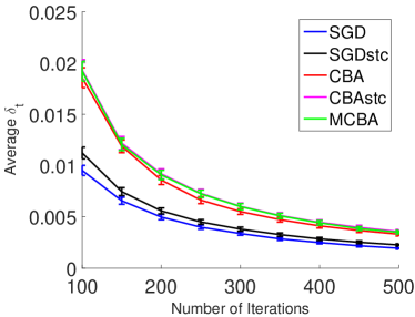
Refer to caption
Refer to caption
Refer to caption
Refer to caption
Figure 1: The convergence of the average relative optimality gap for different algorithms for the four instances. First row: h1​(x,ΞΎ)subscriptβ„Ž1π‘₯πœ‰h_{1}(x,\xi); Second row: h2​(x,ΞΎ)subscriptβ„Ž2π‘₯πœ‰h_{2}(x,\xi). First column: ΞΎβˆΌπ’°β€‹[50,150]similar-toπœ‰π’°50150\xi\sim\mathcal{U}[50,150]; Second column: ΞΎβˆΌπ’©β€‹(100,100)similar-toπœ‰π’©100100\xi\sim\mathcal{N}(100,100).

In Figure 1, the xπ‘₯x-axis represents the number of iterations and the y𝑦y-axis represents the average relative optimality gap for each algorithm. The curves CBA and SGD represent the results of CBA and SGD with Ξ·t=1/tsubscriptπœ‚π‘‘1𝑑\eta_{t}=1/\sqrt{t} respectively while the curves CBAstc and SGDstc represent the results of CBA and SGD with Ξ·t=1/(μ​t)subscriptπœ‚π‘‘1πœ‡π‘‘\eta_{t}=1/(\mu t) respectively. The curve MCBA represents the results of the MCBA algorithm. In each of the curves, the bar at each point represents the standard error of the corresponding Ξ΄tsubscript𝛿𝑑\delta_{t}. As one can see, the standard errors are fairly small. Thus the test results are quite stable in these numerical experiments. We also present the average computation time of all algorithms in TableΒ 3.

h1​(x,ΞΎ)subscriptβ„Ž1π‘₯πœ‰h_{1}(x,\xi) h2​(x,ΞΎ)subscriptβ„Ž2π‘₯πœ‰h_{2}(x,\xi)
Algorithm ΞΎβˆΌπ’°β€‹[50,150]similar-toπœ‰π’°50150\xi\sim\mathcal{U}[50,150] ΞΎβˆΌπ’©β€‹(100,100)similar-toπœ‰π’©100100\xi\sim\mathcal{N}(100,100) ΞΎβˆΌπ’°β€‹[50,150]similar-toπœ‰π’°50150\xi\sim\mathcal{U}[50,150] ΞΎβˆΌπ’©β€‹(100,100)similar-toπœ‰π’©100100\xi\sim\mathcal{N}(100,100)
SGD 0.008 0.007 0.010 0.040
SGDstc 0.007 0.007 0.009 0.038
CBA 0.011 0.018 0.013 0.049
CBAstc 0.011 0.017 0.013 0.045
MCBA 0.013 0.021 0.017 0.055
Table 1: The computation time (in seconds) of different algorithms for 500 iterations for the four instances.

From the results shown in Figure 1, we can see that all of CBA, CBAstc and MCBA converge quite fast in these problems. Even though they use much less information than the SGD and the SGDstc methods, it takes only about twice as many iterations to get the same accuracy. As shown in TableΒ 3, the computation time for 500 iterations is less than 0.10.10.1 seconds in each algorithm and the time is not much different across different algorithms. (This short runtime is because of the low dimensionality of the problems.) Moreover, in our tests, CBA, CBAstc and MCBA have quite similar performance despite their different theoretical guarantees.101010 Note that in Figure 1, the CBA and the CBAstc sometimes perform even better than the MCBA despite the worse theoretical guarantee. In fact, this is common in convex optimization literature for such types of (restarting) methods. For example, Chen etΒ al. (2012) proposed a stochastic gradient method called MORDA, which improves ORDA in the same paper in theoretical convergence rate using a similar restarting technique to our MCBA method. However, in the fourth column of Table 2 in Chen etΒ al. (2012), the objective value in MORDA is higher than that in ORDA. Similarly, Lan and Ghadimi (2012) developed a stochastic gradient method called Multistage AC-SA, which improves AC-SA in theoretical convergence rate but not necessarily in numerical performance (see Table 4.3 in Lan and Ghadimi 2012).

5.2 Choices of fβˆ’subscript𝑓f_{-} and f+subscript𝑓f_{+}

In this section, we perform some additional tests to study the impact of different choices of fβˆ’subscript𝑓f_{-} and f+subscript𝑓f_{+} on the performance of the CBA. We still consider the two objective functions considered in the last section, but we focus on the case in which ΞΎβˆΌπ’©β€‹(100,100)similar-toπœ‰π’©100100\xi\sim\mathcal{N}(100,100). First we keep fβˆ’subscript𝑓f_{-} and f+subscript𝑓f_{+} to be exponential distributions (as in Example 3.2) and see how the performance is affected by different values of Ξ»βˆ’=Ξ»+=Ξ»subscriptπœ†subscriptπœ†πœ†\lambda_{-}=\lambda_{+}=\lambda. The results are shown in Figure 2.

Refer to caption
Refer to caption
Figure 2: The impact of Ξ»πœ†\lambda in f+subscript𝑓f_{+} and fβˆ’subscript𝑓f_{-} to different algorithms, measured by the average relative optimality gap after 500 iterations. Left: h1​(x,ΞΎ)subscriptβ„Ž1π‘₯πœ‰h_{1}(x,\xi); Right: h2​(x,ΞΎ)subscriptβ„Ž2π‘₯πœ‰h_{2}(x,\xi). In both cases, ΞΎβˆΌπ’©β€‹(100,100)similar-toπœ‰π’©100100\xi\sim\mathcal{N}(100,100).

In Figure 2, the xπ‘₯x-axis represents the value of log2⁑λsubscript2πœ†\log_{2}\lambda while the y𝑦y-axis represents the relative optimality gap Ξ΄Tsubscript𝛿𝑇\delta_{T} after 500500500 iterations evaluated as the average value of 200020002000 independent trials (again the bars show the standard error in these trials). The influences of different values of Ξ»πœ†\lambda in fβˆ’subscript𝑓f_{-} and f+subscript𝑓f_{+} are presented for the CBA, the CBAstc and the MCBA algorithms. We can see that the value of Ξ»πœ†\lambda does influence the convergence speed of the algorithms. Particularly, in both figures in Figure 2, the optimality gap after T=500𝑇500T=500 iterations decreases first as Ξ»πœ†\lambda increases but starts to increase when Ξ»πœ†\lambda is large. Moreover, the influence is relatively small when Ξ»πœ†\lambda is small but is large when Ξ»πœ†\lambda is large. And the influence is more pronounced for the CBAstc algorithm. In our setting, the best performance is obtained around Ξ»=2βˆ’4=0.0625πœ†superscript240.0625\lambda=2^{-4}=0.0625 for all algorithms.

In Section 3, we provided the optimal choice of fβˆ’subscript𝑓f_{-} and f+subscript𝑓f_{+} in (13) and (14). In FigureΒ 3, we present the difference in the performances of the CBA when fβˆ’subscript𝑓f_{-} and f+subscript𝑓f_{+} are chosen optimally versus when they are chosen as exponential distributions with Ξ»βˆ’=Ξ»+=0.0625subscriptπœ†subscriptπœ†0.0625\lambda_{-}=\lambda_{+}=0.0625. In this experiment, we choose h​(x,ΞΎ)=h1​(x,ΞΎ)β„Žπ‘₯πœ‰subscriptβ„Ž1π‘₯πœ‰h(x,\xi)=h_{1}(x,\xi) and run the CBA for 500 iterations and compute the average relative optimality gap Ξ΄500subscript𝛿500\delta_{500} over 200020002000 independent trials. The results are plotted in Figure 3.
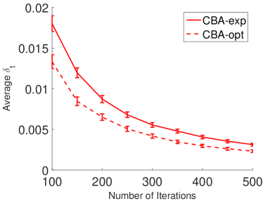
Refer to caption
Refer to caption
Figure 3: The convergence of the average relative optimality gap in CBA when choosing f+subscript𝑓f_{+} and fβˆ’subscript𝑓f_{-} to be the exponential distribution and the optimal distribution in (13) and (14). Left: ΞΎβˆΌπ’°β€‹[50,150]similar-toπœ‰π’°50150\xi\sim\mathcal{U}[50,150]; Right: ΞΎβˆΌπ’©β€‹(100,100)similar-toπœ‰π’©100100\xi\sim\mathcal{N}(100,100). In both cases, h​(x,ΞΎ)=(xβˆ’ΞΎ)2β„Žπ‘₯πœ‰superscriptπ‘₯πœ‰2h(x,\xi)=(x-\xi)^{2}.

In Figure 3, we can see that the optimal choice of fβˆ’subscript𝑓f_{-} and f+subscript𝑓f_{+} does improve the performance of the CBA, which confirms our analysis in Section 3. However, the improvement is not essential yet generating samples from the optimal distribution is much more time consuming. For example, when ΞΎβˆΌπ’©β€‹(100,100)similar-toπœ‰π’©100100\xi\sim\mathcal{N}(100,100), the computational time is less than 0.050.050.05 seconds when using exponential distribution but about 111 second when using the optimal distribution. Therefore, as we discussed in the end of Section 3, one can just choose a simple distribution in practice.

5.3 Mini-Batch Method with Additional Comparisons

In this section, we numerically test how the performance of CBA depends on the sample size S𝑆S in the mini-batch technique described in SectionΒ 4.3. The instances and the choice of parameters are all identical to SectionΒ 5.1. We present the convergence of CBA with S=1,2,5,10,100𝑆12510100S=1,2,5,10,100 in FigureΒ 4 and the associated runtimes in TableΒ 2. According to the figures, one additional comparison (i.e. S=2𝑆2S=2) with z𝑧z can improve the convergence of AlgorithmΒ 1 in all four instances. Although increasing S𝑆S can still improve the performance further, the effect diminishes quickly. This is because the noise in the stochastic gradient is generated from the sample noise of both ΞΎπœ‰\xi and z𝑧z. The mini-batch technique for sampling z𝑧z does not help reduce the noise due to ΞΎπœ‰\xi, which eventually dominates the noise due to z𝑧z when S𝑆S is large enough.111111In Appendix 10, we also present numerical results of convergence with mini-batch method with respect to runtime of the algorithm. The results show that choosing a small batch size can usually lead to fastest convergence (in terms of time). This is because of the tradeoff between the reduced number of iterations required in the mini-batch method and the increased computational efforts required in each iteration. Although a similar mini-batch technique can be applied to ΞΎπœ‰\xi, it might not be practical when applying our algorithm in practice. For example, when ΞΎπœ‰\xi represents the ideal product of a customer, creating a mini-batch for ΞΎπœ‰\xi means asking different customers’ preference without updating the solution, which is not consistent with the setting of online optimization where the solution is updated after the visit of each customer.
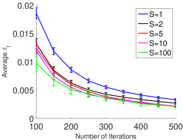
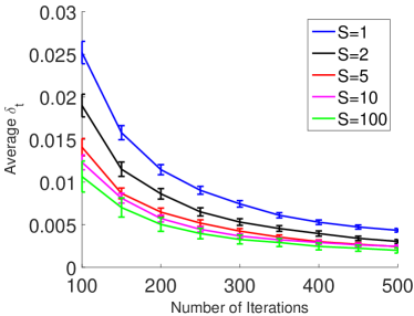
Refer to caption
Refer to caption
Refer to caption
Refer to caption
Figure 4: The convergence of the average relative optimality gap in CBA when using different numbers of comparisons (S𝑆S). First row: h1​(x,ΞΎ)subscriptβ„Ž1π‘₯πœ‰h_{1}(x,\xi); Second row: h2​(x,ΞΎ)subscriptβ„Ž2π‘₯πœ‰h_{2}(x,\xi). First column: ΞΎβˆΌπ’°β€‹[50,150]similar-toπœ‰π’°50150\xi\sim\mathcal{U}[50,150]; Second column: ΞΎβˆΌπ’©β€‹(100,100)similar-toπœ‰π’©100100\xi\sim\mathcal{N}(100,100).
h1​(x,ΞΎ)subscriptβ„Ž1π‘₯πœ‰h_{1}(x,\xi) h2​(x,ΞΎ)subscriptβ„Ž2π‘₯πœ‰h_{2}(x,\xi)
S𝑆S ΞΎβˆΌπ’°β€‹[50,150]similar-toπœ‰π’°50150\xi\sim\mathcal{U}[50,150] ΞΎβˆΌπ’©β€‹(100,100)similar-toπœ‰π’©100100\xi\sim\mathcal{N}(100,100) ΞΎβˆΌπ’°β€‹[50,150]similar-toπœ‰π’°50150\xi\sim\mathcal{U}[50,150] ΞΎβˆΌπ’©β€‹(100,100)similar-toπœ‰π’©100100\xi\sim\mathcal{N}(100,100)
1 0.011 0.018 0.013 0.049
2 0.015 0.022 0.020 0.053
5 0.021 0.025 0.022 0.057
10 0.026 0.033 0.029 0.064
100 0.117 0.158 0.125 0.175
Table 2: The computation time (in seconds) of CBA for 500 iterations when using different numbers of comparisons (S𝑆S) per iteration.

5.4 Multi-Dimensional Problems

In this section, we conduct numerical experiments to test the performance of the CBA-QP and the MCBA-QP on the multi-dimensional stochastic quadratic programΒ (15). To generate a testing instance ofΒ (15), we first generate a dΓ—d𝑑𝑑d\times d matrix Qβ€²superscript𝑄′Q^{\prime} where each entry is sampled from an i.i.d. standard normal distribution 𝒩​(0,1)𝒩01\mathcal{N}(0,1) and then set Q=(Qβ€²)βŠ€β€‹Qβ€²/d+Id𝑄superscriptsuperscript𝑄′topsuperscript𝑄′𝑑subscript𝐼𝑑Q=(Q^{\prime})^{\top}Q^{\prime}/d+I_{d} inΒ (15), where Idsubscript𝐼𝑑I_{d} is a dΓ—d𝑑𝑑d\times d identity matrix. We choose the random variable ΞΎπœ‰\xi in (15) with a multivariate normal distribution 𝒩​(100β€‹πŸd,502​Id)𝒩100subscript1𝑑superscript502subscript𝐼𝑑\mathcal{N}(100\mathbf{1}_{d},50^{2}I_{d}), where 𝟏dsubscript1𝑑\mathbf{1}_{d} is the all-one vector in ℝdsuperscriptℝ𝑑\mathbb{R}^{d}. It is easy to show that, with this choice, AssumptionΒ 4.1 holds and we have 𝔼​exp⁑(β€–ΞΎβ€–2)≀σ¯𝔼subscriptnormπœ‰2¯𝜎\mathbb{E}\exp(\|\xi\|_{2})\leq\bar{\sigma} for some σ¯>0¯𝜎0\bar{\sigma}>0 so that we can choose f𝑓f in AlgorithmsΒ 4.4 andΒ 4.5 to be an exponential distribution in order to guarantee (C4) according to ExampleΒ 4.2. More specifically, we choose f𝑓f to be the exponential distribution (16) with Ξ»=2βˆ’4=0.0625πœ†superscript240.0625\lambda=2^{-4}=0.0625 (same as Ξ»+subscriptπœ†\lambda_{+} and Ξ»βˆ’subscriptπœ†\lambda_{-} in SectionΒ 5.1). Finally, we choose the feasible set ofΒ (15) to be the box 𝒳=∏1d[50,150]𝒳superscriptsubscriptproduct1𝑑50150\mathcal{X}=\prod_{1}^{d}[50,150].

We compare the performance of the SGD, CBA-QP and MCBA-QP methods. In the SGD method, each iteration computes xt+1=Proj𝒳​(xtβˆ’Ξ·t​Q​(xtβˆ’ΞΎt))subscriptπ‘₯𝑑1subscriptProj𝒳subscriptπ‘₯𝑑subscriptπœ‚π‘‘π‘„subscriptπ‘₯𝑑subscriptπœ‰π‘‘x_{t+1}=\text{Proj}_{\mathcal{X}}\left(x_{t}-\eta_{t}Q(x_{t}-\xi_{t})\right) where ΞΎtsubscriptπœ‰π‘‘\xi_{t} is sampled from the distribution of ΞΎπœ‰\xi and Q​(xtβˆ’ΞΎt)𝑄subscriptπ‘₯𝑑subscriptπœ‰π‘‘Q(x_{t}-\xi_{t}) is the gradient of h​(x,ΞΎ)β„Žπ‘₯πœ‰h(x,\xi) with respect to xπ‘₯x. As suggested by Proposition 4.4, we choose Ξ·t=1/(μ​t+L)subscriptπœ‚π‘‘1πœ‡π‘‘πΏ\eta_{t}=1/(\mu t+L) in CBA-QP where ΞΌπœ‡\mu and L𝐿L are the smallest and largest eigenvalues of Q𝑄Q, respectively. For MCBA, we choose Ξ·tk=12k+1​μ+Lsuperscriptsubscriptπœ‚π‘‘π‘˜1superscript2π‘˜1πœ‡πΏ\eta_{t}^{k}=\frac{1}{2^{k+1}\mu+L} and Tk=2k+3+4subscriptπ‘‡π‘˜superscript2π‘˜34T_{k}=2^{k+3}+4 as suggested by Proposition 4.5. In the experiments, we apply the same step lengths in the SGD method as in the CBA-QP method.

We randomly generate Q𝑄Q in the aforementioned method, start each algorithm at the same initial point x1subscriptπ‘₯1x_{1} that is uniformly randomly sampled in the box 𝒳𝒳\mathcal{X}, and run each algorithm for T=2000𝑇2000T=2000 iterations. We report the average relative optimality gap Ξ΄t=H​(xΒ―t)βˆ’H​(xβˆ—)H​(xβˆ—)subscript𝛿𝑑𝐻subscriptΒ―π‘₯𝑑𝐻superscriptπ‘₯𝐻superscriptπ‘₯\delta_{t}=\frac{H(\bar{x}_{t})-H(x^{*})}{H(x^{*})} and its standard error over 200020002000 independent trails for each t𝑑t. We run these experiments with the dimension d=5𝑑5d=5 and d=20𝑑20d=20. The results are reported in Figure 5.
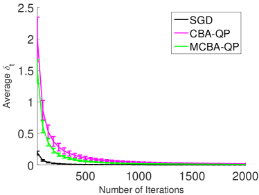
Refer to caption
Refer to caption
Figure 5: The convergence of the average relative optimality gap for different algorithms for the multi-dimensional quadratic programΒ (15). Left: d=5𝑑5d=5; Right: d=20𝑑20d=20.

From the results shown in Figure 5, we see that even though CBA-QP and MCBA-QP use much less information than the SGD method, they can eventually find a solution with an accuracy comparable to SGD. As shown in TableΒ 3, the computation time for 2000 iterations is less than one second in each algorithm and the time is not much different across different algorithms. (This short runtime is because of the low dimensionality of the problems.) Moreover, in our tests, MCBA-QP has a faster convergence rate than CBA-QP which is consistent with PropositionΒ 4.4 andΒ 4.5. However, CBA-QP and MCBA-QP converge more slowly than SGD. This is because SGD utilizes the information of ΞΎπœ‰\xi with the full dimension while CBA-QP and MCBA-QP can only exploit information along a random direction u𝑒u. This difference is more significant as the dimension increases, which is confirmed by Figure 5.

Algorithm d=5𝑑5d=5 d=20𝑑20d=20
SGD 0.236 0.344
CBA-QP 0.391 0.490
MCBA-QP 0.440 0.585
Table 3: The computation time (in seconds) of different algorithms for 2000 iterations for the four instances.

6 Concluding Remarks

In this paper, we considered a stochastic optimization problem when neither the underlying uncertain parameters nor the objective value at the sampled point can be observed. Instead, the decision maker can only access to comparative information between the sample point and two chosen decision points in each iteration. We proposed an algorithm that gives unbiased gradient estimates for this problem, which achieves the same asymptotic convergence rate as standard stochastic gradient methods. Numerical experiments demonstrate that our proposed algorithm is efficient.

There is one remark we would like to make. In this paper, we assumed that ΞΎπœ‰\xi follows a continuous distribution. However, we only need that in each iteration, the probability that ΞΎt=xtsubscriptπœ‰π‘‘subscriptπ‘₯𝑑\xi_{t}=x_{t} is 00. This can be guaranteed by only requiring ℙ​(ΞΎ=β„“)=ℙ​(ΞΎ=u)=0β„™πœ‰β„“β„™πœ‰π‘’0{\mathbb{P}}(\xi=\ell)={\mathbb{P}}(\xi=u)=0, and then in the CBA, adding a small and decaying random perturbation to g​(xt,ΞΎt,zt)𝑔subscriptπ‘₯𝑑subscriptπœ‰π‘‘subscript𝑧𝑑g(x_{t},\xi_{t},z_{t}) (for example, a uniform distribution on [βˆ’1/2t,1/2t]1superscript2𝑑1superscript2𝑑[-1/2^{t},1/2^{t}] in iteration t𝑑t). By doing this, one can still use the same analysis, and the same performance guarantee holds for the modified algorithm.

There are several future directions of research. First, for multi-dimensional problems, we only considered convex quadratic problems in this paper (as mentioned in Section 4.1, we can also generalize our method to separable objective function cases). It would be of interest to see whether the ideas and techniques can be generalized to more general multi-dimensional settings. Second, in this paper, we assumed that the distribution of ΞΎπœ‰\xi is stationary over time, and the comparative information is always reported accurately. However, in practice, the distribution of ΞΎπœ‰\xi may change over time or the comparative information may be reported in a noisy fashion. It would be interesting to see whether we could extend our discussions to consider such situations. Finally, our paper only considers a continuous decision setting, i.e., we assumed that all the decision variables as well as the test variables can take any continuous values. In many practical situations, the decision variables may only be chosen from a finite set. It is worth further research to see whether a similar idea can be applied in such settings.

Acknowledgments

The authors thank the editor-in-chief, the associated editor and three anonymous referees for many useful suggestions and feedback. Xi Chen was supported by the NSF IIS-18454444, the Alibaba Innovation Research Award, and the Bloomberg Data Science Research Grant.

References

  • Asmussen and Glynn (2007) Asmussen, S., P.Β W. Glynn. 2007. Stochastic Simulation. Springer.
  • Attouch etΒ al. (2010) Attouch, H., J.Β Bolte, P.Β Redont, A.Β Soubeyran. 2010. Proximal alternating minimization and projection methods for nonconvex problems: An approach based on the Kurdyka-Lojasiewicz inequality. Mathematics of Operations Research 35(2) 438–457.
  • Ban and Rudin (2018) Ban, G.-Y., C.Β Rudin. 2018. The big data newsvendor: Practical insights from machine learning. Operations Research Forthcoming.
  • Bensoussan etΒ al. (2007) Bensoussan, A., M.Β Γ‡akanyildirim, S.Β P. Sethi. 2007. A multiperiod newsvendor problem with partially observed demand. Mathematics of Operations Research 32(2) 322–344.
  • Besbes and Muharremoglu (2013) Besbes, O., A.Β Muharremoglu. 2013. On implications of demand censoring in the newsvendor problem. Management Science 59(6) 1407–1424.
  • Bolte etΒ al. (2007) Bolte, J., A.Β Daniilidis, A.Β Lewis. 2007. The Ε‚ojasiewicz inequality for nonsmooth subanalytic functions with applications to subgradient dynamical systems. SIAM Journal on Optimization 17(4) 1205–1223.
  • Bolte etΒ al. (2014) Bolte, J., S.Β Sabach, M.Β Teboulle. 2014. Proximal alternating linearized minimization or nonconvex and nonsmooth problems. Mathematical Programming 146(1-2) 459–494.
  • Cachon and Swinney (2011) Cachon, G., R.Β Swinney. 2011. The value of fast fashion: Quick response, enhanced design, and strategic consumer behavior. Management Science 57(4) 579–595.
  • Candogan etΒ al. (2012) Candogan, O., K.Β Bimpikis, A.Β Ozdaglar. 2012. Optimal pricing in networks with externalities. Operations Research 60(4) 883–905.
  • Cesa-Bianchi and Lugosi (2006) Cesa-Bianchi, N., G.Β Lugosi. 2006. Prediction, Learning, and Games. Cambridge University Press.
  • Chen etΒ al. (2012) Chen, X., Q.Β Lin, J.Β Pena. 2012. Optimal regularized dual averaging methods for stochastic optimization. Advances in Neural Information Processing Systems 25. 395–403.
  • Davis and Drusvyatskiy (2018) Davis, D., D.Β Drusvyatskiy. 2018. Stochastic subgradient method converges at the rate O​(kβˆ’1/4)𝑂superscriptπ‘˜14{O}(k^{-1/4}) on weakly convex functions. Working Paper.
  • den Boer (2015) den Boer, A.Β V. 2015. Dynamic pricing and learning: Historical origins, current research, and new directions. Surveys in Operations Research and Management Science 20(1) 1–18.
  • Ding etΒ al. (2002) Ding, X., M.Β Puterman, A.Β Bisi. 2002. The censored newsvendor and the optimal acquisition of information. Operations Research 50(3) 517–527.
  • Duchi etΒ al. (2011) Duchi, J., E.Β Hazan, Y.Β Singer. 2011. Adaptive subgradient methods for online learning and stochastic optimization. Journal of Machine Learning Research 12 2121–2159.
  • Duchi and Singer (2009) Duchi, J., Y.Β Singer. 2009. Efficient online and batch learning using forward-backward splitting. Journal of Machine Learning Research 10 2873–2898.
  • Gupta and Denton (2008) Gupta, D., B.Β Denton. 2008. Appointment scheduling in health care: Challenges and opportunities. IIE Transactions 40 800–819.
  • Halman etΒ al. (2012) Halman, N., J.Β Orlin, D.Β Simchi-Levi. 2012. Approximating the nonlinear newsvendor and single-item stochastic lot-sizing problems when data is given by an oracle. Operations Research 60(2) 429–446.
  • Hazan and Kale (2014) Hazan, E., S.Β Kale. 2014. Beyond the regret minimization barrier: Optimal algorithms for stochastic strongly-convex optimization. Journal of Machine Learning Research 15 2489–2512.
  • Hu etΒ al. (2009) Hu, C., J.Β T. Kwok, W.Β Pan. 2009. Accelerated gradient methods for stochastic optimization and online learning. Advances in Neural Information Processing Systems 22. 781–789.
  • Karimi etΒ al. (2016) Karimi, H., J.Β Nutini, M.Β Schmidt. 2016. Linear convergence of gradient and proximal-gradient methods under the Polyak-Lojasiewicz condition. Joint European Conference on Machine Learning and Knowledge Discovery in Databases. Springer, 795–811.
  • Kiefer and Wolfowitz (1952) Kiefer, J., J.Β Wolfowitz. 1952. Stochastic estimation of the maximum of a regression function. The Annals of Mathematical Statistics 23(3) 462–466.
  • Kolker (2017) Kolker, A. 2017. The Optimal Workforce Staffing Solutions With Random Patient Demand in Healthcare Settings, chap. 322. IGI Global Information Science, 3711 – 3724.
  • Lan (2012) Lan, G. 2012. An optimal method for stochastic composite optimization. Mathematical Programming 133(1-2) 365–397.
  • Lan and Ghadimi (2012) Lan, G., S.Β Ghadimi. 2012. Optimal stochastic approximation algorithms for strongly convex stochastic composite optimization, Part I: A generic algorithmic framework. SIAM Journal on Optimization 22(4) 1469–1492.
  • Lan and Ghadimi (2013) Lan, G., S.Β Ghadimi. 2013. Optimal stochastic approximation algorithms for strongly convex stochastic composite optimization, Part II: Shrinking procedures and optimal algorithms. SIAM Journal on Optimization 23(4) 2061–2089.
  • Levi etΒ al. (2015) Levi, R., G.Β Perakis, J.Β Uichanco. 2015. The data-driven newsvendor problem: New bounds and insights. Operations Research 63(6) 1294–1306.
  • Li etΒ al. (2017) Li, Q., Y.Β Zhou, Y.Β Liang, P.Β K. Varshney. 2017. Convergence analysis of proximal gradient with momentum for nonconvex optimization. Working Paper.
  • Lin etΒ al. (2011) Lin, Q., X.Β Chen, J.Β Pena. 2011. A sparsity preserving stochastic gradient method for composite optimization. Tech. rep., Carnegie Mellon University.
  • Nemirovski etΒ al. (2009) Nemirovski, A., A.Β Juditsky, G.Β Lan, A.Β Shapiro. 2009. Robust stochastic approximation approach to stochastic programming. SIAM Journal on Optimization 19(4) 1574–1609.
  • Nemirovski and Yudin (1983) Nemirovski, A., D.Β Yudin. 1983. Problem Complexity and Method Efficiency in Optimization. Weily, New York.
  • Noll (2014) Noll, D. 2014. Convergence of non-smooth descent methods using the Kurdyka–Lojasiewicz inequality. Journal of Optimization Theory and Applications 160(2) 553–572.
  • Rakhlin etΒ al. (2012) Rakhlin, A., O.Β Shamir, K.Β Sridharan. 2012. Making gradient descent optimal for strongly convex stochastic optimization. Proceedings of the 29th International Conference on Machine Learning. 449–456.
  • Robbins and Monro (1951) Robbins, H., S.Β Monro. 1951. A stochastic approximation method. The Annals of Mathematical Statistics 22(3) 400–407.
  • Shalev-Shwartz (2012) Shalev-Shwartz, S. 2012. Online learning and online convex optimization. Foundations and Trends in Machine Learning 4(2) 107–194.
  • Shamir and Zhang (2013) Shamir, O., T.Β Zhang. 2013. Stochastic gradient descent for non-smooth optimization: Convergence results and optimal averaging schemes. Proceedings of the 30th International Conference on Machine Learning. 71–79.
  • Shapiro etΒ al. (2014) Shapiro, A., D.Β Dentcheva, A.Β Ruszczynski. 2014. Lectures on Stochastic Programming: Modeling and Theory. SIAM.
  • Widder (1990) Widder, D.Β V. 1990. Advanced Calculus. Dover Publication Inc.
  • Xiao (2010) Xiao, L. 2010. Dual averaging methods for regularized stochastic learning and online optimization. Journal of Machine Learning Research 11 2543–2596.
  • Xu and Yin (2017) Xu, Y., W.Β Yin. 2017. A globally convergent algorithm for nonconvex optimization based on block coordinate update. Journal of Scientific Computing 72(2) 700–734.
  • Zinkevich (2003) Zinkevich, M. 2003. Online convex programming and generalized infinitesimal gradient ascent. Proceedings of the 20th International Conference on Machine Learning. 928–936.
\APPENDICES

7 Proofs of PropositionΒ 2.2, 2.3 and 2.4

Proof of PropositionΒ 2.2. We prove the proposition by considering the case when Assumption A5(a) or A5(b) holds respectively. For the ease of notation, we shall use 𝔼tsubscript𝔼𝑑\mathbb{E}_{t} to denote the conditional expectation taken over ΞΎtsubscriptπœ‰π‘‘\xi_{t} and ztsubscript𝑧𝑑z_{t} conditioning on ΞΎ1,z1,ΞΎ2,z2,…,ΞΎtβˆ’1,ztβˆ’1subscriptπœ‰1subscript𝑧1subscriptπœ‰2subscript𝑧2…subscriptπœ‰π‘‘1subscript𝑧𝑑1\xi_{1},z_{1},\xi_{2},z_{2},\dots,\xi_{t-1},z_{t-1}.

1. When Assumption A5(a) holds (based on Nemirovski etΒ al. 2009, Duchi and Singer 2009):

According to (10), we have

(xt+1βˆ’xβˆ—)2superscriptsubscriptπ‘₯𝑑1superscriptπ‘₯2\displaystyle(x_{t+1}-x^{*})^{2} =\displaystyle= (Proj[β„“,u]​(xtβˆ’Ξ·t​g​(xt,ΞΎt,zt))βˆ’Proj[β„“,u]​(xβˆ—))2superscriptsubscriptProjℓ𝑒subscriptπ‘₯𝑑subscriptπœ‚π‘‘π‘”subscriptπ‘₯𝑑subscriptπœ‰π‘‘subscript𝑧𝑑subscriptProjℓ𝑒superscriptπ‘₯2\displaystyle(\text{Proj}_{[\ell,u]}(x_{t}-\eta_{t}g(x_{t},\xi_{t},z_{t}))-\text{Proj}_{[\ell,u]}(x^{*}))^{2} (23)
≀\displaystyle\leq (xtβˆ’Ξ·t​g​(xt,ΞΎt,zt)βˆ’xβˆ—)2superscriptsubscriptπ‘₯𝑑subscriptπœ‚π‘‘π‘”subscriptπ‘₯𝑑subscriptπœ‰π‘‘subscript𝑧𝑑superscriptπ‘₯2\displaystyle(x_{t}-\eta_{t}g(x_{t},\xi_{t},z_{t})-x^{*})^{2}
=\displaystyle= (xtβˆ’xβˆ—)2βˆ’2​ηt​g​(xt,ΞΎt,zt)​(xtβˆ’xβˆ—)+Ξ·t2​(g​(xt,ΞΎt,zt))2.superscriptsubscriptπ‘₯𝑑superscriptπ‘₯22subscriptπœ‚π‘‘π‘”subscriptπ‘₯𝑑subscriptπœ‰π‘‘subscript𝑧𝑑subscriptπ‘₯𝑑superscriptπ‘₯superscriptsubscriptπœ‚π‘‘2superscript𝑔subscriptπ‘₯𝑑subscriptπœ‰π‘‘subscript𝑧𝑑2\displaystyle(x_{t}-x^{*})^{2}-2\eta_{t}g(x_{t},\xi_{t},z_{t})(x_{t}-x^{*})+\eta_{t}^{2}(g(x_{t},\xi_{t},z_{t}))^{2}.

Taking expectation of (23) over ΞΎtsubscriptπœ‰π‘‘\xi_{t} and ztsubscript𝑧𝑑z_{t}, we have

𝔼t​(xt+1βˆ’xβˆ—)2subscript𝔼𝑑superscriptsubscriptπ‘₯𝑑1superscriptπ‘₯2\displaystyle\mathbb{E}_{t}(x_{t+1}-x^{*})^{2} =\displaystyle= (xtβˆ’xβˆ—)2βˆ’2​ηt​H′​(xt)​(xtβˆ’xβˆ—)+Ξ·t2​𝔼t​(g​(xt,ΞΎt,zt))2superscriptsubscriptπ‘₯𝑑superscriptπ‘₯22subscriptπœ‚π‘‘superscript𝐻′subscriptπ‘₯𝑑subscriptπ‘₯𝑑superscriptπ‘₯superscriptsubscriptπœ‚π‘‘2subscript𝔼𝑑superscript𝑔subscriptπ‘₯𝑑subscriptπœ‰π‘‘subscript𝑧𝑑2\displaystyle(x_{t}-x^{*})^{2}-2\eta_{t}H^{\prime}(x_{t})(x_{t}-x^{*})+\eta_{t}^{2}\mathbb{E}_{t}(g(x_{t},\xi_{t},z_{t}))^{2} (24)
≀\displaystyle\leq (1βˆ’Ξ·t​μ)​(xtβˆ’xβˆ—)2βˆ’2​ηt​(H​(xt)βˆ’H​(xβˆ—))+Ξ·t2​𝔼t​(g​(xt,ΞΎt,zt))2,1subscriptπœ‚π‘‘πœ‡superscriptsubscriptπ‘₯𝑑superscriptπ‘₯22subscriptπœ‚π‘‘π»subscriptπ‘₯𝑑𝐻superscriptπ‘₯superscriptsubscriptπœ‚π‘‘2subscript𝔼𝑑superscript𝑔subscriptπ‘₯𝑑subscriptπœ‰π‘‘subscript𝑧𝑑2\displaystyle(1-\eta_{t}\mu)(x_{t}-x^{*})^{2}-2\eta_{t}(H(x_{t})-H(x^{*}))+\eta_{t}^{2}\mathbb{E}_{t}(g(x_{t},\xi_{t},z_{t}))^{2},

where the first equality is because of Proposition 2.1 and the last inequality is because of (3) (H​(β‹…)𝐻⋅H(\cdot) is ΞΌπœ‡\mu-convex). According to the third statement in Proposition 2.1, (24) implies that

H​(xt)βˆ’H​(xβˆ—)𝐻subscriptπ‘₯𝑑𝐻superscriptπ‘₯\displaystyle H(x_{t})-H(x^{*}) ≀\displaystyle\leq 1βˆ’Ξ·t​μ2​ηt​(xtβˆ’xβˆ—)2βˆ’12​ηt​𝔼t​(xt+1βˆ’xβˆ—)2+Ξ·t​G22.1subscriptπœ‚π‘‘πœ‡2subscriptπœ‚π‘‘superscriptsubscriptπ‘₯𝑑superscriptπ‘₯212subscriptπœ‚π‘‘subscript𝔼𝑑superscriptsubscriptπ‘₯𝑑1superscriptπ‘₯2subscriptπœ‚π‘‘superscript𝐺22\displaystyle\frac{1-\eta_{t}\mu}{2\eta_{t}}(x_{t}-x^{*})^{2}-\frac{1}{2\eta_{t}}\mathbb{E}_{t}(x_{t+1}-x^{*})^{2}+\frac{\eta_{t}G^{2}}{2}. (25)

If ΞΌ=0πœ‡0\mu=0 and we choose Ξ·t=1Tsubscriptπœ‚π‘‘1𝑇\eta_{t}=\frac{1}{\sqrt{T}}, then summing (25) for t=1,2,…,T𝑑12…𝑇t=1,2,\dots,T and taking expectation give

T​𝔼​(H​(xΒ―T)βˆ’H​(xβˆ—))β‰€βˆ‘t=1T𝔼​(H​(xt)βˆ’H​(xβˆ—))≀T2​(x1βˆ’xβˆ—)2+T​G22.𝑇𝔼𝐻subscriptΒ―π‘₯𝑇𝐻superscriptπ‘₯superscriptsubscript𝑑1𝑇𝔼𝐻subscriptπ‘₯𝑑𝐻superscriptπ‘₯𝑇2superscriptsubscriptπ‘₯1superscriptπ‘₯2𝑇superscript𝐺22\displaystyle T\mathbb{E}(H(\bar{x}_{T})-H(x^{*}))\leq\sum_{t=1}^{T}\mathbb{E}(H(x_{t})-H(x^{*}))\leq\frac{\sqrt{T}}{2}(x_{1}-x^{*})^{2}+\frac{\sqrt{T}G^{2}}{2}.

The desired result for this part is obtained by dividing this inequality by T𝑇T. In addition, if both u𝑒u and β„“β„“\ell are finite and we choose Ξ·t=1tsubscriptπœ‚π‘‘1𝑑\eta_{t}=\frac{1}{\sqrt{t}}, then summing (25) for t=1,2,…,T𝑑12…𝑇t=1,2,\dots,T and taking expectation give

T​𝔼​(H​(xΒ―T)βˆ’H​(xβˆ—))β‰€βˆ‘t=1T𝔼​(H​(xt)βˆ’H​(xβˆ—))β‰€βˆ‘t=1Ttβˆ’tβˆ’12​(xtβˆ’xβˆ—)2+βˆ‘t=1TG22​t.𝑇𝔼𝐻subscriptΒ―π‘₯𝑇𝐻superscriptπ‘₯superscriptsubscript𝑑1𝑇𝔼𝐻subscriptπ‘₯𝑑𝐻superscriptπ‘₯superscriptsubscript𝑑1𝑇𝑑𝑑12superscriptsubscriptπ‘₯𝑑superscriptπ‘₯2superscriptsubscript𝑑1𝑇superscript𝐺22𝑑\displaystyle T\mathbb{E}(H(\bar{x}_{T})-H(x^{*}))\leq\sum_{t=1}^{T}\mathbb{E}(H(x_{t})-H(x^{*}))\leq\sum_{t=1}^{T}\frac{\sqrt{t}-\sqrt{t-1}}{2}(x_{t}-x^{*})^{2}+\sum_{t=1}^{T}\frac{G^{2}}{2\sqrt{t}}.

Note that (xtβˆ’xβˆ—)2≀(uβˆ’β„“)2superscriptsubscriptπ‘₯𝑑superscriptπ‘₯2superscript𝑒ℓ2(x_{t}-x^{*})^{2}\leq(u-\ell)^{2} and βˆ‘t=1T1tβ‰€βˆ«0T1x​𝑑x=2​Tsuperscriptsubscript𝑑1𝑇1𝑑superscriptsubscript0𝑇1π‘₯differential-dπ‘₯2𝑇\sum_{t=1}^{T}\frac{1}{\sqrt{t}}\leq\int_{0}^{T}\frac{1}{\sqrt{x}}dx=2\sqrt{T} so that the above inequality implies

T​𝔼​(H​(xΒ―T)βˆ’H​(xβˆ—))β‰€βˆ‘t=1T𝔼​(H​(xt)βˆ’H​(xβˆ—))≀T2​(uβˆ’β„“)2+T​G2.𝑇𝔼𝐻subscriptΒ―π‘₯𝑇𝐻superscriptπ‘₯superscriptsubscript𝑑1𝑇𝔼𝐻subscriptπ‘₯𝑑𝐻superscriptπ‘₯𝑇2superscript𝑒ℓ2𝑇superscript𝐺2\displaystyle T\mathbb{E}(H(\bar{x}_{T})-H(x^{*}))\leq\sum_{t=1}^{T}\mathbb{E}(H(x_{t})-H(x^{*}))\leq\frac{\sqrt{T}}{2}(u-\ell)^{2}+\sqrt{T}G^{2}.

The desired result for this part is obtained by dividing this inequality by T𝑇T.

2. When Assumption A5(b) holds (based on Lan 2012):

The ΞΌπœ‡\mu-convexity property (3) of H​(β‹…)𝐻⋅H(\cdot) implies that

H​(xβˆ—)𝐻superscriptπ‘₯\displaystyle H(x^{*}) β‰₯\displaystyle\geq H​(xt)+H′​(xt)​(xβˆ—βˆ’xt)+ΞΌ2​(xβˆ—βˆ’xt)2𝐻subscriptπ‘₯𝑑superscript𝐻′subscriptπ‘₯𝑑superscriptπ‘₯subscriptπ‘₯π‘‘πœ‡2superscriptsuperscriptπ‘₯subscriptπ‘₯𝑑2\displaystyle H(x_{t})+H^{\prime}(x_{t})(x^{*}-x_{t})+\frac{\mu}{2}(x^{*}-x_{t})^{2} (26)
=\displaystyle= H​(xt)+𝔼t​[g​(xt,ΞΎt,zt)​(xβˆ—βˆ’xt)]+ΞΌ2​(xβˆ—βˆ’xt)2𝐻subscriptπ‘₯𝑑subscript𝔼𝑑delimited-[]𝑔subscriptπ‘₯𝑑subscriptπœ‰π‘‘subscript𝑧𝑑superscriptπ‘₯subscriptπ‘₯π‘‘πœ‡2superscriptsuperscriptπ‘₯subscriptπ‘₯𝑑2\displaystyle H(x_{t})+\mathbb{E}_{t}[g(x_{t},\xi_{t},z_{t})(x^{*}-x_{t})]+\frac{\mu}{2}(x^{*}-x_{t})^{2}
=\displaystyle= H​(xt)+𝔼t​[(g​(xt,ΞΎt,zt)βˆ’H′​(xt))​(xt+1βˆ’xt)]+H′​(xt)​(xt+1βˆ’xt)𝐻subscriptπ‘₯𝑑subscript𝔼𝑑delimited-[]𝑔subscriptπ‘₯𝑑subscriptπœ‰π‘‘subscript𝑧𝑑superscript𝐻′subscriptπ‘₯𝑑subscriptπ‘₯𝑑1subscriptπ‘₯𝑑superscript𝐻′subscriptπ‘₯𝑑subscriptπ‘₯𝑑1subscriptπ‘₯𝑑\displaystyle H(x_{t})+\mathbb{E}_{t}[(g(x_{t},\xi_{t},z_{t})-H^{\prime}(x_{t}))(x_{t+1}-x_{t})]+H^{\prime}(x_{t})(x_{t+1}-x_{t})
+𝔼t​[g​(xt,ΞΎt,zt)​(xβˆ—βˆ’xt+1)]+ΞΌ2​(xβˆ—βˆ’xt)2,subscript𝔼𝑑delimited-[]𝑔subscriptπ‘₯𝑑subscriptπœ‰π‘‘subscript𝑧𝑑superscriptπ‘₯subscriptπ‘₯𝑑1πœ‡2superscriptsuperscriptπ‘₯subscriptπ‘₯𝑑2\displaystyle+\mathbb{E}_{t}[g(x_{t},\xi_{t},z_{t})(x^{*}-x_{t+1})]+\frac{\mu}{2}(x^{*}-x_{t})^{2},

where the first equality is because of Proposition 2.1. By Assumption A5(b), H′​(x)superscript𝐻′π‘₯H^{\prime}(x) is L𝐿L-Lipschitz continuous, thus

H​(xt+1)𝐻subscriptπ‘₯𝑑1\displaystyle H(x_{t+1}) ≀\displaystyle\leq H​(xt)+H′​(xt)​(xt+1βˆ’xt)+L2​(xt+1βˆ’xt)2𝐻subscriptπ‘₯𝑑superscript𝐻′subscriptπ‘₯𝑑subscriptπ‘₯𝑑1subscriptπ‘₯𝑑𝐿2superscriptsubscriptπ‘₯𝑑1subscriptπ‘₯𝑑2\displaystyle H(x_{t})+H^{\prime}(x_{t})(x_{t+1}-x_{t})+\frac{L}{2}(x_{t+1}-x_{t})^{2}

which, together with (26), implies that

H​(xβˆ—)𝐻superscriptπ‘₯\displaystyle H(x^{*}) β‰₯\displaystyle\geq 𝔼t​H​(xt+1)+𝔼t​[(g​(xt,ΞΎt,zt)βˆ’H′​(xt))​(xt+1βˆ’xt)]βˆ’L2​𝔼t​(xt+1βˆ’xt)2subscript𝔼𝑑𝐻subscriptπ‘₯𝑑1subscript𝔼𝑑delimited-[]𝑔subscriptπ‘₯𝑑subscriptπœ‰π‘‘subscript𝑧𝑑superscript𝐻′subscriptπ‘₯𝑑subscriptπ‘₯𝑑1subscriptπ‘₯𝑑𝐿2subscript𝔼𝑑superscriptsubscriptπ‘₯𝑑1subscriptπ‘₯𝑑2\displaystyle\mathbb{E}_{t}H(x_{t+1})+\mathbb{E}_{t}[(g(x_{t},\xi_{t},z_{t})-H^{\prime}(x_{t}))(x_{t+1}-x_{t})]-\frac{L}{2}\mathbb{E}_{t}(x_{t+1}-x_{t})^{2}
+𝔼t​[g​(xt,ΞΎt,zt)​(xβˆ—βˆ’xt+1)]+ΞΌ2​(xβˆ—βˆ’xt)2subscript𝔼𝑑delimited-[]𝑔subscriptπ‘₯𝑑subscriptπœ‰π‘‘subscript𝑧𝑑superscriptπ‘₯subscriptπ‘₯𝑑1πœ‡2superscriptsuperscriptπ‘₯subscriptπ‘₯𝑑2\displaystyle+\mathbb{E}_{t}[g(x_{t},\xi_{t},z_{t})(x^{*}-x_{t+1})]+\frac{\mu}{2}(x^{*}-x_{t})^{2}
β‰₯\displaystyle\geq 𝔼t​H​(xt+1)βˆ’12​at​𝔼t​(g​(xt,ΞΎt,zt)βˆ’H′​(xt))2βˆ’L+at2​𝔼t​(xt+1βˆ’xt)2subscript𝔼𝑑𝐻subscriptπ‘₯𝑑112subscriptπ‘Žπ‘‘subscript𝔼𝑑superscript𝑔subscriptπ‘₯𝑑subscriptπœ‰π‘‘subscript𝑧𝑑superscript𝐻′subscriptπ‘₯𝑑2𝐿subscriptπ‘Žπ‘‘2subscript𝔼𝑑superscriptsubscriptπ‘₯𝑑1subscriptπ‘₯𝑑2\displaystyle\mathbb{E}_{t}H(x_{t+1})-\frac{1}{2a_{t}}\mathbb{E}_{t}(g(x_{t},\xi_{t},z_{t})-H^{\prime}(x_{t}))^{2}-\frac{L+a_{t}}{2}\mathbb{E}_{t}(x_{t+1}-x_{t})^{2}
+𝔼t​[g​(xt,ΞΎt,zt)​(xβˆ—βˆ’xt+1)]+ΞΌ2​(xβˆ—βˆ’xt)2subscript𝔼𝑑delimited-[]𝑔subscriptπ‘₯𝑑subscriptπœ‰π‘‘subscript𝑧𝑑superscriptπ‘₯subscriptπ‘₯𝑑1πœ‡2superscriptsuperscriptπ‘₯subscriptπ‘₯𝑑2\displaystyle+\mathbb{E}_{t}[g(x_{t},\xi_{t},z_{t})(x^{*}-x_{t+1})]+\frac{\mu}{2}(x^{*}-x_{t})^{2}
β‰₯\displaystyle\geq 𝔼t​H​(xt+1)βˆ’Οƒ22​atβˆ’L+at2​𝔼t​(xt+1βˆ’xt)2+𝔼t​[g​(xt,ΞΎt,zt)​(xβˆ—βˆ’xt+1)]+ΞΌ2​(xβˆ—βˆ’xt)2,subscript𝔼𝑑𝐻subscriptπ‘₯𝑑1superscript𝜎22subscriptπ‘Žπ‘‘πΏsubscriptπ‘Žπ‘‘2subscript𝔼𝑑superscriptsubscriptπ‘₯𝑑1subscriptπ‘₯𝑑2subscript𝔼𝑑delimited-[]𝑔subscriptπ‘₯𝑑subscriptπœ‰π‘‘subscript𝑧𝑑superscriptπ‘₯subscriptπ‘₯𝑑1πœ‡2superscriptsuperscriptπ‘₯subscriptπ‘₯𝑑2\displaystyle\mathbb{E}_{t}H(x_{t+1})-\frac{\sigma^{2}}{2a_{t}}-\frac{L+a_{t}}{2}\mathbb{E}_{t}(x_{t+1}-x_{t})^{2}+\mathbb{E}_{t}[g(x_{t},\xi_{t},z_{t})(x^{*}-x_{t+1})]+\frac{\mu}{2}(x^{*}-x_{t})^{2},

where atsubscriptπ‘Žπ‘‘a_{t} is a positive constant, the second inequality is due to Young’s inequality, namely, x​y≀x22​a+a​y22π‘₯𝑦superscriptπ‘₯22π‘Žπ‘Žsuperscript𝑦22xy\leq\frac{x^{2}}{2a}+\frac{ay^{2}}{2} for any a>0π‘Ž0a>0, and the last equality is due to the third statement of Proposition 2.1. We will determine the value of atsubscriptπ‘Žπ‘‘a_{t} later but we always ensure that atsubscriptπ‘Žπ‘‘a_{t} and Ξ·tsubscriptπœ‚π‘‘\eta_{t} satisfy

L+at2βˆ’12​ηt≀0.𝐿subscriptπ‘Žπ‘‘212subscriptπœ‚π‘‘0\displaystyle\frac{L+a_{t}}{2}-\frac{1}{2\eta_{t}}\leq 0. (27)

By the optimality of xt+1subscriptπ‘₯𝑑1x_{t+1} as a solution to the projection problemΒ (10), we have

(xt+1βˆ’xt+Ξ·t​g​(xt,ΞΎt,zt))​(xβˆ—βˆ’xt+1)β‰₯0.subscriptπ‘₯𝑑1subscriptπ‘₯𝑑subscriptπœ‚π‘‘π‘”subscriptπ‘₯𝑑subscriptπœ‰π‘‘subscript𝑧𝑑superscriptπ‘₯subscriptπ‘₯𝑑10\displaystyle(x_{t+1}-x_{t}+\eta_{t}g(x_{t},\xi_{t},z_{t}))(x^{*}-x_{t+1})\geq 0.

Thus we have

H​(xβˆ—)𝐻superscriptπ‘₯\displaystyle H(x^{*}) β‰₯\displaystyle\geq 𝔼t​H​(xt+1)βˆ’Οƒ22​atβˆ’L+at2​𝔼t​(xt+1βˆ’xt)2+1Ξ·t​𝔼t​[(xt+1βˆ’xt)​(xt+1βˆ’xβˆ—)]+ΞΌ2​(xβˆ—βˆ’xt)2subscript𝔼𝑑𝐻subscriptπ‘₯𝑑1superscript𝜎22subscriptπ‘Žπ‘‘πΏsubscriptπ‘Žπ‘‘2subscript𝔼𝑑superscriptsubscriptπ‘₯𝑑1subscriptπ‘₯𝑑21subscriptπœ‚π‘‘subscript𝔼𝑑delimited-[]subscriptπ‘₯𝑑1subscriptπ‘₯𝑑subscriptπ‘₯𝑑1superscriptπ‘₯πœ‡2superscriptsuperscriptπ‘₯subscriptπ‘₯𝑑2\displaystyle\mathbb{E}_{t}H(x_{t+1})-\frac{\sigma^{2}}{2a_{t}}-\frac{L+a_{t}}{2}\mathbb{E}_{t}(x_{t+1}-x_{t})^{2}+\frac{1}{\eta_{t}}\mathbb{E}_{t}[(x_{t+1}-x_{t})(x_{t+1}-x^{*})]+\frac{\mu}{2}(x^{*}-x_{t})^{2} (28)
=\displaystyle= 𝔼t​H​(xt+1)βˆ’Οƒ22​atβˆ’(L+at2βˆ’12​ηt)​𝔼t​(xt+1βˆ’xt)2subscript𝔼𝑑𝐻subscriptπ‘₯𝑑1superscript𝜎22subscriptπ‘Žπ‘‘πΏsubscriptπ‘Žπ‘‘212subscriptπœ‚π‘‘subscript𝔼𝑑superscriptsubscriptπ‘₯𝑑1subscriptπ‘₯𝑑2\displaystyle\mathbb{E}_{t}H(x_{t+1})-\frac{\sigma^{2}}{2a_{t}}-\left(\frac{L+a_{t}}{2}-\frac{1}{2\eta_{t}}\right)\mathbb{E}_{t}(x_{t+1}-x_{t})^{2}
+12​ηt​𝔼t​(xt+1βˆ’xβˆ—)2βˆ’(12​ηtβˆ’ΞΌ2)​𝔼t​(xtβˆ’xβˆ—)212subscriptπœ‚π‘‘subscript𝔼𝑑superscriptsubscriptπ‘₯𝑑1superscriptπ‘₯212subscriptπœ‚π‘‘πœ‡2subscript𝔼𝑑superscriptsubscriptπ‘₯𝑑superscriptπ‘₯2\displaystyle+\frac{1}{2\eta_{t}}\mathbb{E}_{t}(x_{t+1}-x^{*})^{2}-\left(\frac{1}{2\eta_{t}}-\frac{\mu}{2}\right)\mathbb{E}_{t}(x_{t}-x^{*})^{2}
β‰₯\displaystyle\geq 𝔼t​H​(xt+1)βˆ’Οƒ22​at+12​ηt​𝔼t​(xt+1βˆ’xβˆ—)2βˆ’(12​ηtβˆ’ΞΌ2)​𝔼t​(xtβˆ’xβˆ—)2,subscript𝔼𝑑𝐻subscriptπ‘₯𝑑1superscript𝜎22subscriptπ‘Žπ‘‘12subscriptπœ‚π‘‘subscript𝔼𝑑superscriptsubscriptπ‘₯𝑑1superscriptπ‘₯212subscriptπœ‚π‘‘πœ‡2subscript𝔼𝑑superscriptsubscriptπ‘₯𝑑superscriptπ‘₯2\displaystyle\mathbb{E}_{t}H(x_{t+1})-\frac{\sigma^{2}}{2a_{t}}+\frac{1}{2\eta_{t}}\mathbb{E}_{t}(x_{t+1}-x^{*})^{2}-\left(\frac{1}{2\eta_{t}}-\frac{\mu}{2}\right)\mathbb{E}_{t}(x_{t}-x^{*})^{2},

where the second inequality is from (27).

If ΞΌ=0πœ‡0\mu=0 and we choose Ξ·t=1L+Tsubscriptπœ‚π‘‘1𝐿𝑇\eta_{t}=\frac{1}{L+\sqrt{T}} and at=Tsubscriptπ‘Žπ‘‘π‘‡a_{t}=\sqrt{T} so that (27) is satisfied. Summing (28) for t=1,2,…,Tβˆ’1𝑑12…𝑇1t=1,2,\dots,T-1 and organizing terms give

T​𝔼​(H​(xΒ―T)βˆ’H​(xβˆ—))β‰€βˆ‘t=1T𝔼​(H​(xt)βˆ’H​(xβˆ—))≀L+T2​(x1βˆ’xβˆ—)2+H​(x1)βˆ’H​(xβˆ—)+T​σ22.𝑇𝔼𝐻subscriptΒ―π‘₯𝑇𝐻superscriptπ‘₯superscriptsubscript𝑑1𝑇𝔼𝐻subscriptπ‘₯𝑑𝐻superscriptπ‘₯𝐿𝑇2superscriptsubscriptπ‘₯1superscriptπ‘₯2𝐻subscriptπ‘₯1𝐻superscriptπ‘₯𝑇superscript𝜎22\displaystyle T\mathbb{E}(H(\bar{x}_{T})-H(x^{*}))\leq\sum_{t=1}^{T}\mathbb{E}(H(x_{t})-H(x^{*}))\leq\frac{L+\sqrt{T}}{2}(x_{1}-x^{*})^{2}+H(x_{1})-H(x^{*})+\frac{\sqrt{T}\sigma^{2}}{2}.

The desired result for this part is obtained by dividing this inequality by T𝑇T. In addition, if both u𝑒u and β„“β„“\ell are finite and we choose Ξ·t=1L+tsubscriptπœ‚π‘‘1𝐿𝑑\eta_{t}=\frac{1}{L+\sqrt{t}} and at=tsubscriptπ‘Žπ‘‘π‘‘a_{t}=\sqrt{t}, then summing (28) for t=1,2,…,Tβˆ’1𝑑12…𝑇1t=1,2,\dots,T-1 and taking expectation give

T​𝔼​(H​(xΒ―T)βˆ’H​(xβˆ—))𝑇𝔼𝐻subscriptΒ―π‘₯𝑇𝐻superscriptπ‘₯\displaystyle T\mathbb{E}(H(\bar{x}_{T})-H(x^{*})) ≀\displaystyle\leq βˆ‘t=1T𝔼​(H​(xt)βˆ’H​(xβˆ—))superscriptsubscript𝑑1𝑇𝔼𝐻subscriptπ‘₯𝑑𝐻superscriptπ‘₯\displaystyle\sum_{t=1}^{T}\mathbb{E}(H(x_{t})-H(x^{*}))
≀\displaystyle\leq βˆ‘t=1Tβˆ’1tβˆ’tβˆ’12​(xtβˆ’xβˆ—)2+H​(x1)βˆ’H​(xβˆ—)+L2​(x1βˆ’xβˆ—)2+βˆ‘t=1Tβˆ’1Οƒ22​t.superscriptsubscript𝑑1𝑇1𝑑𝑑12superscriptsubscriptπ‘₯𝑑superscriptπ‘₯2𝐻subscriptπ‘₯1𝐻superscriptπ‘₯𝐿2superscriptsubscriptπ‘₯1superscriptπ‘₯2superscriptsubscript𝑑1𝑇1superscript𝜎22𝑑\displaystyle\sum_{t=1}^{T-1}\frac{\sqrt{t}-\sqrt{t-1}}{2}(x_{t}-x^{*})^{2}+H(x_{1})-H(x^{*})+\frac{L}{2}(x_{1}-x^{*})^{2}+\sum_{t=1}^{T-1}\frac{\sigma^{2}}{2\sqrt{t}}.

Note that (xtβˆ’xβˆ—)2≀(uβˆ’β„“)2superscriptsubscriptπ‘₯𝑑superscriptπ‘₯2superscript𝑒ℓ2(x_{t}-x^{*})^{2}\leq(u-\ell)^{2} and βˆ‘t=1Tβˆ’11tβ‰€βˆ«0T1x​𝑑x=2​Tsuperscriptsubscript𝑑1𝑇11𝑑superscriptsubscript0𝑇1π‘₯differential-dπ‘₯2𝑇\sum_{t=1}^{T-1}\frac{1}{\sqrt{t}}\leq\int_{0}^{T}\frac{1}{\sqrt{x}}dx=2\sqrt{T} so that the above inequality implies

T​𝔼​(H​(xΒ―T)βˆ’H​(xβˆ—))β‰€βˆ‘t=1T𝔼​(H​(xt)βˆ’H​(xβˆ—))≀T2​(uβˆ’β„“)2+H​(x1)βˆ’H​(xβˆ—)+L2​(x1βˆ’xβˆ—)2+T​σ2.𝑇𝔼𝐻subscriptΒ―π‘₯𝑇𝐻superscriptπ‘₯superscriptsubscript𝑑1𝑇𝔼𝐻subscriptπ‘₯𝑑𝐻superscriptπ‘₯𝑇2superscript𝑒ℓ2𝐻subscriptπ‘₯1𝐻superscriptπ‘₯𝐿2superscriptsubscriptπ‘₯1superscriptπ‘₯2𝑇superscript𝜎2\displaystyle T\mathbb{E}(H(\bar{x}_{T})-H(x^{*}))\leq\sum_{t=1}^{T}\mathbb{E}(H(x_{t})-H(x^{*}))\leq\frac{\sqrt{T}}{2}(u-\ell)^{2}+H(x_{1})-H(x^{*})+\frac{L}{2}(x_{1}-x^{*})^{2}+\sqrt{T}\sigma^{2}.

The desired result for this part is obtained by dividing this inequality by T𝑇T. β–‘β–‘\hfill\Box

Proof of Proposition 2.3. Similar as to the proof of Proposition 2.2, we consider the case when Assumption A5(a) or A5(b) holds respectively, and use 𝔼tsubscript𝔼𝑑\mathbb{E}_{t} to denote the conditional expectation taken over ΞΎtsubscriptπœ‰π‘‘\xi_{t} and ztsubscript𝑧𝑑z_{t} conditioning on ΞΎ1,z1,ΞΎ2,z2,…,ΞΎtβˆ’1,ztβˆ’1subscriptπœ‰1subscript𝑧1subscriptπœ‰2subscript𝑧2…subscriptπœ‰π‘‘1subscript𝑧𝑑1\xi_{1},z_{1},\xi_{2},z_{2},\dots,\xi_{t-1},z_{t-1}.

1. When Assumption A5(a) holds: We can still show (25) using exactly the same argument in the proof of Proposition 2.2.

If ΞΌ>0πœ‡0\mu>0 and we choose Ξ·t=1μ​tsubscriptπœ‚π‘‘1πœ‡π‘‘\eta_{t}=\frac{1}{\mu t}, summing (25) for t=1,2,…,T𝑑12…𝑇t=1,2,\dots,T gives

T​𝔼​(H​(xΒ―T)βˆ’H​(xβˆ—))β‰€βˆ‘t=1T𝔼​(H​(xt)βˆ’H​(xβˆ—))β‰€βˆ‘t=1TG22​μ​t.𝑇𝔼𝐻subscriptΒ―π‘₯𝑇𝐻superscriptπ‘₯superscriptsubscript𝑑1𝑇𝔼𝐻subscriptπ‘₯𝑑𝐻superscriptπ‘₯superscriptsubscript𝑑1𝑇superscript𝐺22πœ‡π‘‘\displaystyle T\mathbb{E}(H(\bar{x}_{T})-H(x^{*}))\leq\sum_{t=1}^{T}\mathbb{E}(H(x_{t})-H(x^{*}))\leq\sum_{t=1}^{T}\frac{G^{2}}{2\mu t}.

The desired result for this part is obtained by dividing this inequality by T𝑇T and using the fact that βˆ‘t=1T1t≀log⁑T+1superscriptsubscript𝑑1𝑇1𝑑𝑇1\sum_{t=1}^{T}\frac{1}{t}\leq\log T+1.

2. When Assumption A5(b) holds: Using exactly the same argument in the proof of Proposition 2.2, we can show that (28) holds for any positive constant atsubscriptπ‘Žπ‘‘a_{t} that satisfies (27).

If ΞΌ>0πœ‡0\mu>0 and we choose Ξ·t=1μ​t+Lsubscriptπœ‚π‘‘1πœ‡π‘‘πΏ\eta_{t}=\frac{1}{\mu t+L} and at=μ​tsubscriptπ‘Žπ‘‘πœ‡π‘‘a_{t}=\mu t so that (27) is satisfied. Summing (28) for t=1,2,…,Tβˆ’1𝑑12…𝑇1t=1,2,\dots,T-1 gives

T​𝔼​(H​(xΒ―T)βˆ’H​(xβˆ—))β‰€βˆ‘t=1T𝔼​(H​(xt)βˆ’H​(xβˆ—))β‰€βˆ‘t=1TΟƒ22​μ​t+H​(x1)βˆ’H​(xβˆ—)+L​(x1βˆ’xβˆ—)22.𝑇𝔼𝐻subscriptΒ―π‘₯𝑇𝐻superscriptπ‘₯superscriptsubscript𝑑1𝑇𝔼𝐻subscriptπ‘₯𝑑𝐻superscriptπ‘₯superscriptsubscript𝑑1𝑇superscript𝜎22πœ‡π‘‘π»subscriptπ‘₯1𝐻superscriptπ‘₯𝐿superscriptsubscriptπ‘₯1superscriptπ‘₯22\displaystyle T\mathbb{E}(H(\bar{x}_{T})-H(x^{*}))\leq\sum_{t=1}^{T}\mathbb{E}(H(x_{t})-H(x^{*}))\leq\sum_{t=1}^{T}\frac{\sigma^{2}}{2\mu t}+H(x_{1})-H(x^{*})+\frac{L(x_{1}-x^{*})^{2}}{2}.

The desired result for this part is obtained by dividing this inequality by T𝑇T and using the fact that βˆ‘t=1T1t≀log⁑T+1superscriptsubscript𝑑1𝑇1𝑑𝑇1\sum_{t=1}^{T}\frac{1}{t}\leq\log T+1. β–‘β–‘\hfill\Box

Before we prove Proposition 2.4, we first introduce the following lemma:

Lemma 7.1

If Assumption A5(a) holds, then by choosing Ξ·t=η∈(0,+∞)subscriptπœ‚π‘‘πœ‚0\eta_{t}=\eta\in(0,+\infty), the CBA ensures that

𝔼​(H​(xΒ―T)βˆ’H​(xβˆ—))≀(x1βˆ’xβˆ—)22​η​T+η​G22.𝔼𝐻subscriptΒ―π‘₯𝑇𝐻superscriptπ‘₯superscriptsubscriptπ‘₯1superscriptπ‘₯22πœ‚π‘‡πœ‚superscript𝐺22\displaystyle\mathbb{E}(H(\bar{x}_{T})-H(x^{*}))\leq\frac{(x_{1}-x^{*})^{2}}{2\eta T}+\frac{\eta G^{2}}{2}.

If Assumption A5(b) holds, then by choosing Ξ·t=η∈(0,1L)subscriptπœ‚π‘‘πœ‚01𝐿\eta_{t}=\eta\in(0,\frac{1}{L}) and at=1Ξ·tβˆ’Lsubscriptπ‘Žπ‘‘1subscriptπœ‚π‘‘πΏa_{t}=\frac{1}{\eta_{t}}-L, the CBA ensures that

𝔼​(H​(xΒ―T)βˆ’H​(xβˆ—))≀(x1βˆ’xβˆ—)22​η​T+H​(x1)βˆ’H​(xβˆ—)T+Οƒ21/Ξ·βˆ’L.𝔼𝐻subscriptΒ―π‘₯𝑇𝐻superscriptπ‘₯superscriptsubscriptπ‘₯1superscriptπ‘₯22πœ‚π‘‡π»subscriptπ‘₯1𝐻superscriptπ‘₯𝑇superscript𝜎21πœ‚πΏ\displaystyle\mathbb{E}(H(\bar{x}_{T})-H(x^{*}))\leq\frac{(x_{1}-x^{*})^{2}}{2\eta T}+\frac{H(x_{1})-H(x^{*})}{T}+\frac{\sigma^{2}}{1/\eta-L}.

Proof of Lemma 7.1. When Assumption A5(a) holds, by choosing Ξ·t=η∈(0,∞)subscriptπœ‚π‘‘πœ‚0\eta_{t}=\eta\in(0,\infty) and summing (25) over t=1,2,…,T𝑑12…𝑇t=1,2,\dots,T, we have

T​𝔼​(H​(xΒ―T)βˆ’H​(xβˆ—))β‰€βˆ‘t=1T𝔼​(H​(xt)βˆ’H​(xβˆ—))≀(x1βˆ’xβˆ—)22​η+T​η​G22.𝑇𝔼𝐻subscriptΒ―π‘₯𝑇𝐻superscriptπ‘₯superscriptsubscript𝑑1𝑇𝔼𝐻subscriptπ‘₯𝑑𝐻superscriptπ‘₯superscriptsubscriptπ‘₯1superscriptπ‘₯22πœ‚π‘‡πœ‚superscript𝐺22\displaystyle T\mathbb{E}(H(\bar{x}_{T})-H(x^{*}))\leq\sum_{t=1}^{T}\mathbb{E}(H(x_{t})-H(x^{*}))\leq\frac{(x_{1}-x^{*})^{2}}{2\eta}+\frac{T\eta G^{2}}{2}.

The first conclusion is obtained by dividing this inequality by T𝑇T.

When Assumption A5(b) holds, by setting Ξ·t=η∈(0,1L)subscriptπœ‚π‘‘πœ‚01𝐿\eta_{t}=\eta\in(0,\frac{1}{L}), at=1Ξ·βˆ’Lsubscriptπ‘Žπ‘‘1πœ‚πΏa_{t}=\frac{1}{\eta}-L and summing (28) over t=1,2,…,Tβˆ’1𝑑12…𝑇1t=1,2,\dots,T-1, we have

T​𝔼​(H​(xΒ―T)βˆ’H​(xβˆ—))≀(x1βˆ’xβˆ—)22​η+H​(x1)βˆ’H​(xβˆ—)+T​σ21/Ξ·βˆ’L.𝑇𝔼𝐻subscriptΒ―π‘₯𝑇𝐻superscriptπ‘₯superscriptsubscriptπ‘₯1superscriptπ‘₯22πœ‚π»subscriptπ‘₯1𝐻superscriptπ‘₯𝑇superscript𝜎21πœ‚πΏ\displaystyle T\mathbb{E}(H(\bar{x}_{T})-H(x^{*}))\leq\frac{(x_{1}-x^{*})^{2}}{2\eta}+H(x_{1})-H(x^{*})+\frac{T\sigma^{2}}{1/\eta-L}.

The second conclusion is obtained by dividing this inequality by T𝑇T. β–‘β–‘\hfill\Box

Proof of Proposition 2.4. The optimality of xβˆ—superscriptπ‘₯x^{*} and the ΞΌπœ‡\mu-convexity property (3) of H​(β‹…)𝐻⋅H(\cdot) imply

ΞΌ2​(x^kβˆ’xβˆ—)2≀H​(x^k)βˆ’H​(xβˆ—).πœ‡2superscriptsuperscript^π‘₯π‘˜superscriptπ‘₯2𝐻subscript^π‘₯π‘˜π»superscriptπ‘₯\displaystyle\frac{\mu}{2}(\hat{x}^{k}-x^{*})^{2}\leq H(\hat{x}_{k})-H(x^{*}). (29)

With a slight abuse of notation, let 𝔼ksubscriptπ”Όπ‘˜\mathbb{E}_{k} be the conditional expectation conditioning on x^1,x^2,…,x^ksuperscript^π‘₯1superscript^π‘₯2…superscript^π‘₯π‘˜\hat{x}^{1},\hat{x}^{2},\dots,\hat{x}^{k}.

1. When Assumption A5(a) holds (based on Hazan and Kale 2014):

Define Ξ”k=H​(x^k)βˆ’H​(xβˆ—)subscriptΞ”π‘˜π»superscript^π‘₯π‘˜π»superscriptπ‘₯\Delta_{k}=H(\hat{x}^{k})-H(x^{*}) for kβ‰₯1π‘˜1k\geq 1. In the following, we use induction to show 𝔼​Δk≀Δ1+G2/ΞΌ2kβˆ’1𝔼subscriptΞ”π‘˜subscriptΞ”1superscript𝐺2πœ‡superscript2π‘˜1\mathbb{E}\Delta_{k}\leq\frac{\Delta_{1}+G^{2}/\mu}{2^{k-1}} for kβ‰₯1π‘˜1k\geq 1. Note that this statement holds trivially when k=1π‘˜1k=1. Suppose 𝔼​Δk≀Δ1+G2/ΞΌ2kβˆ’1𝔼subscriptΞ”π‘˜subscriptΞ”1superscript𝐺2πœ‡superscript2π‘˜1\mathbb{E}\Delta_{k}\leq\frac{\Delta_{1}+G^{2}/\mu}{2^{k-1}}. Now we consider 𝔼​Δk+1𝔼subscriptΞ”π‘˜1\mathbb{E}\Delta_{k+1}.

By LemmaΒ 7.1 and Ξ·tk=12k+1​μsuperscriptsubscriptπœ‚π‘‘π‘˜1superscript2π‘˜1πœ‡\eta_{t}^{k}=\frac{1}{2^{k+1}\mu}, we have

𝔼​Δk+1=𝔼k​(H​(x^k+1)βˆ’H​(xβˆ—))≀2k​μ​(x^kβˆ’xβˆ—)2Tk+G22k+2​μ≀2k+1​ΔkTk+G22k+2​μ,𝔼subscriptΞ”π‘˜1subscriptπ”Όπ‘˜π»superscript^π‘₯π‘˜1𝐻superscriptπ‘₯superscript2π‘˜πœ‡superscriptsuperscript^π‘₯π‘˜superscriptπ‘₯2subscriptπ‘‡π‘˜superscript𝐺2superscript2π‘˜2πœ‡superscript2π‘˜1subscriptΞ”π‘˜subscriptπ‘‡π‘˜superscript𝐺2superscript2π‘˜2πœ‡\displaystyle\mathbb{E}\Delta_{k+1}=\mathbb{E}_{k}(H(\hat{x}^{k+1})-H(x^{*}))\leq\frac{2^{k}\mu(\hat{x}^{k}-x^{*})^{2}}{T_{k}}+\frac{G^{2}}{2^{k+2}\mu}\leq\frac{2^{k+1}\Delta_{k}}{T_{k}}+\frac{G^{2}}{2^{k+2}\mu},

where the second inequality is due to (29). Taking expectation over x^1,x^2,…,x^ksuperscript^π‘₯1superscript^π‘₯2…superscript^π‘₯π‘˜\hat{x}^{1},\hat{x}^{2},\dots,\hat{x}^{k} and applying the induction assumption 𝔼​Δk=Ξ”1+G2/ΞΌ2kβˆ’1𝔼subscriptΞ”π‘˜subscriptΞ”1superscript𝐺2πœ‡superscript2π‘˜1\mathbb{E}\Delta_{k}=\frac{\Delta_{1}+G^{2}/\mu}{2^{k-1}}, we have

𝔼​Δk+1≀2k+1​(Ξ”1+G2/ΞΌ)Tk​2kβˆ’1+G22k+2​μ≀Δ12k+1+G22k+1​μ+G22k+2​μ≀Δ1+G2/ΞΌ2k,𝔼subscriptΞ”π‘˜1superscript2π‘˜1subscriptΞ”1superscript𝐺2πœ‡subscriptπ‘‡π‘˜superscript2π‘˜1superscript𝐺2superscript2π‘˜2πœ‡subscriptΞ”1superscript2π‘˜1superscript𝐺2superscript2π‘˜1πœ‡superscript𝐺2superscript2π‘˜2πœ‡subscriptΞ”1superscript𝐺2πœ‡superscript2π‘˜\displaystyle\mathbb{E}\Delta_{k+1}\leq\frac{2^{k+1}(\Delta_{1}+G^{2}/\mu)}{T_{k}2^{k-1}}+\frac{G^{2}}{2^{k+2}\mu}\leq\frac{\Delta_{1}}{2^{k+1}}+\frac{G^{2}}{2^{k+1}\mu}+\frac{G^{2}}{2^{k+2}\mu}\leq\frac{\Delta_{1}+G^{2}/\mu}{2^{k}}, (30)

where we use the facts that Tk=2k+3subscriptπ‘‡π‘˜superscript2π‘˜3T_{k}=2^{k+3}. By induction assumption, 𝔼​Δk≀Δ1+G2/ΞΌ2kβˆ’1𝔼subscriptΞ”π‘˜subscriptΞ”1superscript𝐺2πœ‡superscript2π‘˜1\mathbb{E}\Delta_{k}\leq\frac{\Delta_{1}+G^{2}/\mu}{2^{k-1}} for kβ‰₯1π‘˜1k\geq 1. Since T=βˆ‘k=1KTk=βˆ‘k=1K2k+3≀2K+4𝑇superscriptsubscriptπ‘˜1𝐾subscriptπ‘‡π‘˜superscriptsubscriptπ‘˜1𝐾superscript2π‘˜3superscript2𝐾4T=\sum_{k=1}^{K}T_{k}=\sum_{k=1}^{K}2^{k+3}\leq 2^{K+4}, we have Kβ‰₯log2⁑(T/16)𝐾subscript2𝑇16K\geq\log_{2}(T/16). Let k=Kπ‘˜πΎk=K in (30), we have

𝔼​(H​(x^K+1)βˆ’H​(xβˆ—))=𝔼​ΔK+1≀Δ1+G2/ΞΌ2K≀16​(Ξ”1+G2/ΞΌ)T.𝔼𝐻superscript^π‘₯𝐾1𝐻superscriptπ‘₯𝔼subscriptΔ𝐾1subscriptΞ”1superscript𝐺2πœ‡superscript2𝐾16subscriptΞ”1superscript𝐺2πœ‡π‘‡\displaystyle\mathbb{E}(H(\hat{x}^{K+1})-H(x^{*}))=\mathbb{E}\Delta_{K+1}\leq\frac{\Delta_{1}+G^{2}/\mu}{2^{K}}\leq\frac{16(\Delta_{1}+G^{2}/\mu)}{T}.

2. When Assumption A5(b) holds:

Define Ξ”k=H​(x^k)βˆ’H​(xβˆ—)+L2​(x^kβˆ’xβˆ—)2subscriptΞ”π‘˜π»superscript^π‘₯π‘˜π»superscriptπ‘₯𝐿2superscriptsuperscript^π‘₯π‘˜superscriptπ‘₯2\Delta_{k}=H(\hat{x}^{k})-H(x^{*})+\frac{L}{2}(\hat{x}^{k}-x^{*})^{2} for kβ‰₯1π‘˜1k\geq 1. In the following, we use induction to show 𝔼​Δk≀Δ1+Οƒ2/ΞΌ2kβˆ’1𝔼subscriptΞ”π‘˜subscriptΞ”1superscript𝜎2πœ‡superscript2π‘˜1\mathbb{E}\Delta_{k}\leq\frac{\Delta_{1}+\sigma^{2}/\mu}{2^{k-1}} for kβ‰₯1π‘˜1k\geq 1. Note that this statement holds trivially when k=1π‘˜1k=1. Suppose 𝔼​Δk≀Δ1+Οƒ2/ΞΌ2kβˆ’1𝔼subscriptΞ”π‘˜subscriptΞ”1superscript𝜎2πœ‡superscript2π‘˜1\mathbb{E}\Delta_{k}\leq\frac{\Delta_{1}+\sigma^{2}/\mu}{2^{k-1}}. Now we consider 𝔼​Δk+1𝔼subscriptΞ”π‘˜1\mathbb{E}\Delta_{k+1}.

By LemmaΒ 7.1 and Ξ·tk=12k+1​μ+L∈(0,1L)superscriptsubscriptπœ‚π‘‘π‘˜1superscript2π‘˜1πœ‡πΏ01𝐿\eta_{t}^{k}=\frac{1}{2^{k+1}\mu+L}\in(0,\frac{1}{L}), we have

𝔼​Δk+1=𝔼k​(H​(x^k+1)βˆ’H​(xβˆ—))≀(2k+1​μ+L)​(x^kβˆ’xβˆ—)22​Tk+Ξ”kTk+Οƒ22k+1​μ≀(2k+1+1)​ΔkTk+Οƒ22k+1​μ,𝔼subscriptΞ”π‘˜1subscriptπ”Όπ‘˜π»superscript^π‘₯π‘˜1𝐻superscriptπ‘₯superscript2π‘˜1πœ‡πΏsuperscriptsuperscript^π‘₯π‘˜superscriptπ‘₯22subscriptπ‘‡π‘˜subscriptΞ”π‘˜subscriptπ‘‡π‘˜superscript𝜎2superscript2π‘˜1πœ‡superscript2π‘˜11subscriptΞ”π‘˜subscriptπ‘‡π‘˜superscript𝜎2superscript2π‘˜1πœ‡\displaystyle\mathbb{E}\Delta_{k+1}=\mathbb{E}_{k}(H(\hat{x}^{k+1})-H(x^{*}))\leq\frac{(2^{k+1}\mu+L)(\hat{x}^{k}-x^{*})^{2}}{2T_{k}}+\frac{\Delta_{k}}{T_{k}}+\frac{\sigma^{2}}{2^{k+1}\mu}\leq\left(2^{k+1}+1\right)\frac{\Delta_{k}}{T_{k}}+\frac{\sigma^{2}}{2^{k+1}\mu},

where the second inequality is due to (29). Taking expectation over x^1,x^2,…,x^ksuperscript^π‘₯1superscript^π‘₯2…superscript^π‘₯π‘˜\hat{x}^{1},\hat{x}^{2},\dots,\hat{x}^{k} and applying the induction assumption 𝔼​Δk=Ξ”1+Οƒ2/ΞΌ2kβˆ’1𝔼subscriptΞ”π‘˜subscriptΞ”1superscript𝜎2πœ‡superscript2π‘˜1\mathbb{E}\Delta_{k}=\frac{\Delta_{1}+\sigma^{2}/\mu}{2^{k-1}}, we have

𝔼​Δk+1≀(2k+1+1)​Δ1+Οƒ2/ΞΌTk​2kβˆ’1+Οƒ22k+1​μ≀Δ12k+1+Οƒ22k+1​μ+Οƒ22k+1​μ≀Δ1+Οƒ2/ΞΌ2k,𝔼subscriptΞ”π‘˜1superscript2π‘˜11subscriptΞ”1superscript𝜎2πœ‡subscriptπ‘‡π‘˜superscript2π‘˜1superscript𝜎2superscript2π‘˜1πœ‡subscriptΞ”1superscript2π‘˜1superscript𝜎2superscript2π‘˜1πœ‡superscript𝜎2superscript2π‘˜1πœ‡subscriptΞ”1superscript𝜎2πœ‡superscript2π‘˜\displaystyle\mathbb{E}\Delta_{k+1}\leq\left(2^{k+1}+1\right)\frac{\Delta_{1}+\sigma^{2}/\mu}{T_{k}2^{k-1}}+\frac{\sigma^{2}}{2^{k+1}\mu}\leq\frac{\Delta_{1}}{2^{k+1}}+\frac{\sigma^{2}}{2^{k+1}\mu}+\frac{\sigma^{2}}{2^{k+1}\mu}\leq\frac{\Delta_{1}+\sigma^{2}/\mu}{2^{k}}, (31)

where we use the facts that Tk=2k+3+4subscriptπ‘‡π‘˜superscript2π‘˜34T_{k}=2^{k+3}+4. Thus, 𝔼​Δk≀Δ1+Οƒ2/ΞΌ2kβˆ’1𝔼subscriptΞ”π‘˜subscriptΞ”1superscript𝜎2πœ‡superscript2π‘˜1\mathbb{E}\Delta_{k}\leq\frac{\Delta_{1}+\sigma^{2}/\mu}{2^{k-1}} for kβ‰₯1π‘˜1k\geq 1. Since T=βˆ‘k=1KTk=βˆ‘k=1K(2k+3+4)≀2K+5𝑇superscriptsubscriptπ‘˜1𝐾subscriptπ‘‡π‘˜superscriptsubscriptπ‘˜1𝐾superscript2π‘˜34superscript2𝐾5T=\sum_{k=1}^{K}T_{k}=\sum_{k=1}^{K}\left(2^{k+3}+4\right)\leq 2^{K+5}, we have Kβ‰₯log2⁑(T/32)𝐾subscript2𝑇32K\geq\log_{2}(T/32). Let k=Kπ‘˜πΎk=K in (31), we have

𝔼​(H​(x^K+1)βˆ’H​(xβˆ—))=𝔼​ΔK+1≀Δ1+Οƒ2/ΞΌ2K=32​(Ξ”1+Οƒ2/ΞΌ)T.𝔼𝐻superscript^π‘₯𝐾1𝐻superscriptπ‘₯𝔼subscriptΔ𝐾1subscriptΞ”1superscript𝜎2πœ‡superscript2𝐾32subscriptΞ”1superscript𝜎2πœ‡π‘‡\displaystyle\mathbb{E}(H(\hat{x}^{K+1})-H(x^{*}))=\mathbb{E}\Delta_{K+1}\leq\frac{\Delta_{1}+\sigma^{2}/\mu}{2^{K}}=\frac{32(\Delta_{1}+\sigma^{2}/\mu)}{T}.

Thus the proposition is proved. β–‘β–‘\hfill\Box

8 Proofs of Proposition 4.4 and 4.5

Proof of PropositionΒ 4.4. For the ease of notation, we shall use 𝔼tsubscript𝔼𝑑\mathbb{E}_{t} to denote the conditional expectation taken over ΞΎtsubscriptπœ‰π‘‘\xi_{t}, utsubscript𝑒𝑑u_{t} and ztsubscript𝑧𝑑z_{t} conditioning on ΞΎ1,z1,ut,ΞΎ2,z2,u2​…,ΞΎtβˆ’1,ztβˆ’1,utβˆ’1subscriptπœ‰1subscript𝑧1subscript𝑒𝑑subscriptπœ‰2subscript𝑧2subscript𝑒2…subscriptπœ‰π‘‘1subscript𝑧𝑑1subscript𝑒𝑑1\xi_{1},z_{1},u_{t},\xi_{2},z_{2},u_{2}\dots,\xi_{t-1},z_{t-1},u_{t-1}. The proof is similar to the proof of PropositionΒ 2.2 when Assumption A5(b) holds.

Since ΞΌπœ‡\mu is the smallest eigenvalues of Q𝑄Q and it is positive, H​(β‹…)𝐻⋅H(\cdot) defined in (15) is ΞΌπœ‡\mu-convex, which implies (26) using PropositionΒ 4.3. Moreover, since L𝐿L is the largest eigenvalues of Q𝑄Q, H′​(x)superscript𝐻′π‘₯H^{\prime}(x) is L𝐿L-Lipschitz continuous so that

H​(xt+1)𝐻subscriptπ‘₯𝑑1\displaystyle H(x_{t+1}) ≀\displaystyle\leq H​(xt)+H′​(xt)​(xt+1βˆ’xt)+L2​(xt+1βˆ’xt)2𝐻subscriptπ‘₯𝑑superscript𝐻′subscriptπ‘₯𝑑subscriptπ‘₯𝑑1subscriptπ‘₯𝑑𝐿2superscriptsubscriptπ‘₯𝑑1subscriptπ‘₯𝑑2\displaystyle H(x_{t})+H^{\prime}(x_{t})(x_{t+1}-x_{t})+\frac{L}{2}(x_{t+1}-x_{t})^{2}

which, by PropositionΒ 4.3 and the same argument in the proof of PropositionΒ 2.2, implies that

H​(xβˆ—)𝐻superscriptπ‘₯\displaystyle H(x^{*}) β‰₯\displaystyle\geq 𝔼t​H​(xt+1)βˆ’Οƒ22​atβˆ’L+at2​𝔼t​(xt+1βˆ’xt)2+𝔼t​[g​(xt,ΞΎt,zt)​(xβˆ—βˆ’xt+1)]+ΞΌ2​(xβˆ—βˆ’xt)2,subscript𝔼𝑑𝐻subscriptπ‘₯𝑑1superscript𝜎22subscriptπ‘Žπ‘‘πΏsubscriptπ‘Žπ‘‘2subscript𝔼𝑑superscriptsubscriptπ‘₯𝑑1subscriptπ‘₯𝑑2subscript𝔼𝑑delimited-[]𝑔subscriptπ‘₯𝑑subscriptπœ‰π‘‘subscript𝑧𝑑superscriptπ‘₯subscriptπ‘₯𝑑1πœ‡2superscriptsuperscriptπ‘₯subscriptπ‘₯𝑑2\displaystyle\mathbb{E}_{t}H(x_{t+1})-\frac{\sigma^{2}}{2a_{t}}-\frac{L+a_{t}}{2}\mathbb{E}_{t}(x_{t+1}-x_{t})^{2}+\mathbb{E}_{t}[g(x_{t},\xi_{t},z_{t})(x^{*}-x_{t+1})]+\frac{\mu}{2}(x^{*}-x_{t})^{2},

where atsubscriptπ‘Žπ‘‘a_{t} is a positive constant chosen to satisfy (27).

By the optimality of xt+1subscriptπ‘₯𝑑1x_{t+1} as a solution to the projection problemΒ (19), we have

(xt+1βˆ’xt+Ξ·t​g​(xt,ΞΎt,zt))​(xβˆ—βˆ’xt+1)β‰₯0.subscriptπ‘₯𝑑1subscriptπ‘₯𝑑subscriptπœ‚π‘‘π‘”subscriptπ‘₯𝑑subscriptπœ‰π‘‘subscript𝑧𝑑superscriptπ‘₯subscriptπ‘₯𝑑10\displaystyle(x_{t+1}-x_{t}+\eta_{t}g(x_{t},\xi_{t},z_{t}))(x^{*}-x_{t+1})\geq 0.

Using this inequality and the same argument in the proof of PropositionΒ 2.2 (under Assumption A5(b)), we can show that (28) holds.

Since ΞΌ>0πœ‡0\mu>0 by assumption, we can choose Ξ·t=1μ​t+Lsubscriptπœ‚π‘‘1πœ‡π‘‘πΏ\eta_{t}=\frac{1}{\mu t+L} and at=μ​tsubscriptπ‘Žπ‘‘πœ‡π‘‘a_{t}=\mu t so that (27) is satisfied. Summing (28) for t=1,2,…,Tβˆ’1𝑑12…𝑇1t=1,2,\dots,T-1 gives

T​𝔼​(H​(xΒ―T)βˆ’H​(xβˆ—))β‰€βˆ‘t=1T𝔼​(H​(xt)βˆ’H​(xβˆ—))β‰€βˆ‘t=1TΟƒ22​μ​t+H​(x1)βˆ’H​(xβˆ—)+L​(x1βˆ’xβˆ—)22.𝑇𝔼𝐻subscriptΒ―π‘₯𝑇𝐻superscriptπ‘₯superscriptsubscript𝑑1𝑇𝔼𝐻subscriptπ‘₯𝑑𝐻superscriptπ‘₯superscriptsubscript𝑑1𝑇superscript𝜎22πœ‡π‘‘π»subscriptπ‘₯1𝐻superscriptπ‘₯𝐿superscriptsubscriptπ‘₯1superscriptπ‘₯22\displaystyle T\mathbb{E}(H(\bar{x}_{T})-H(x^{*}))\leq\sum_{t=1}^{T}\mathbb{E}(H(x_{t})-H(x^{*}))\leq\sum_{t=1}^{T}\frac{\sigma^{2}}{2\mu t}+H(x_{1})-H(x^{*})+\frac{L(x_{1}-x^{*})^{2}}{2}.

The conclusion of this proposition is obtained by dividing this inequality by T𝑇T and using the fact that βˆ‘t=1T1t≀log⁑T+1superscriptsubscript𝑑1𝑇1𝑑𝑇1\sum_{t=1}^{T}\frac{1}{t}\leq\log T+1. β–‘β–‘\hfill\Box

Proof of PropositionΒ 4.5. The optimality of xβˆ—superscriptπ‘₯x^{*} and the ΞΌπœ‡\mu-convexity of H​(β‹…)𝐻⋅H(\cdot) imply (29). Let 𝔼ksubscriptπ”Όπ‘˜\mathbb{E}_{k} be the conditional expectation conditioning on x^1,x^2,…,x^ksuperscript^π‘₯1superscript^π‘₯2…superscript^π‘₯π‘˜\hat{x}^{1},\hat{x}^{2},\dots,\hat{x}^{k}.

Following a similar argument to the proof of PropositionΒ 2.4 when Assumption A5(b) holds, we define Ξ”k=H​(x^k)βˆ’H​(xβˆ—)+L2​(x^kβˆ’xβˆ—)2subscriptΞ”π‘˜π»superscript^π‘₯π‘˜π»superscriptπ‘₯𝐿2superscriptsuperscript^π‘₯π‘˜superscriptπ‘₯2\Delta_{k}=H(\hat{x}^{k})-H(x^{*})+\frac{L}{2}(\hat{x}^{k}-x^{*})^{2} for kβ‰₯1π‘˜1k\geq 1. We then use induction to show 𝔼​Δk≀Δ1+Οƒ2/ΞΌ2kβˆ’1𝔼subscriptΞ”π‘˜subscriptΞ”1superscript𝜎2πœ‡superscript2π‘˜1\mathbb{E}\Delta_{k}\leq\frac{\Delta_{1}+\sigma^{2}/\mu}{2^{k-1}} for kβ‰₯1π‘˜1k\geq 1. Note that this statement holds trivially when k=1π‘˜1k=1. Suppose 𝔼​Δk≀Δ1+Οƒ2/ΞΌ2kβˆ’1𝔼subscriptΞ”π‘˜subscriptΞ”1superscript𝜎2πœ‡superscript2π‘˜1\mathbb{E}\Delta_{k}\leq\frac{\Delta_{1}+\sigma^{2}/\mu}{2^{k-1}}. Now we consider 𝔼​Δk+1𝔼subscriptΞ”π‘˜1\mathbb{E}\Delta_{k+1}.

By setting Ξ·tk=12k+1​μ+L∈(0,1L)superscriptsubscriptπœ‚π‘‘π‘˜1superscript2π‘˜1πœ‡πΏ01𝐿\eta_{t}^{k}=\frac{1}{2^{k+1}\mu+L}\in(0,\frac{1}{L}) and summing (28) over t=1,2,…,Tβˆ’1𝑑12…𝑇1t=1,2,\dots,T-1, we have

𝔼​Δk+1=𝔼k​(H​(x^k+1)βˆ’H​(xβˆ—))≀(2k+1​μ+L)​(x^kβˆ’xβˆ—)22​Tk+Ξ”kTk+Οƒ22k+1​μ≀(2k+1+1)​ΔkTk+Οƒ22k+1​μ,𝔼subscriptΞ”π‘˜1subscriptπ”Όπ‘˜π»superscript^π‘₯π‘˜1𝐻superscriptπ‘₯superscript2π‘˜1πœ‡πΏsuperscriptsuperscript^π‘₯π‘˜superscriptπ‘₯22subscriptπ‘‡π‘˜subscriptΞ”π‘˜subscriptπ‘‡π‘˜superscript𝜎2superscript2π‘˜1πœ‡superscript2π‘˜11subscriptΞ”π‘˜subscriptπ‘‡π‘˜superscript𝜎2superscript2π‘˜1πœ‡\displaystyle\mathbb{E}\Delta_{k+1}=\mathbb{E}_{k}(H(\hat{x}^{k+1})-H(x^{*}))\leq\frac{(2^{k+1}\mu+L)(\hat{x}^{k}-x^{*})^{2}}{2T_{k}}+\frac{\Delta_{k}}{T_{k}}+\frac{\sigma^{2}}{2^{k+1}\mu}\leq\left(2^{k+1}+1\right)\frac{\Delta_{k}}{T_{k}}+\frac{\sigma^{2}}{2^{k+1}\mu},

Taking expectation over x^1,x^2,…,x^ksuperscript^π‘₯1superscript^π‘₯2…superscript^π‘₯π‘˜\hat{x}^{1},\hat{x}^{2},\dots,\hat{x}^{k} and applying the induction assumption 𝔼​Δk=Ξ”1+Οƒ2/ΞΌ2kβˆ’1𝔼subscriptΞ”π‘˜subscriptΞ”1superscript𝜎2πœ‡superscript2π‘˜1\mathbb{E}\Delta_{k}=\frac{\Delta_{1}+\sigma^{2}/\mu}{2^{k-1}}, we can obtain (31). Thus, 𝔼​Δk≀Δ1+Οƒ2/ΞΌ2kβˆ’1𝔼subscriptΞ”π‘˜subscriptΞ”1superscript𝜎2πœ‡superscript2π‘˜1\mathbb{E}\Delta_{k}\leq\frac{\Delta_{1}+\sigma^{2}/\mu}{2^{k-1}} for kβ‰₯1π‘˜1k\geq 1. Since T=βˆ‘k=1KTk=βˆ‘k=1K(2k+3+4)≀2K+5𝑇superscriptsubscriptπ‘˜1𝐾subscriptπ‘‡π‘˜superscriptsubscriptπ‘˜1𝐾superscript2π‘˜34superscript2𝐾5T=\sum_{k=1}^{K}T_{k}=\sum_{k=1}^{K}\left(2^{k+3}+4\right)\leq 2^{K+5}, we have Kβ‰₯log2⁑(T/32)𝐾subscript2𝑇32K\geq\log_{2}(T/32). Let k=Kπ‘˜πΎk=K in (31), we have

𝔼​(H​(x^K+1)βˆ’H​(xβˆ—))=𝔼​ΔK+1≀Δ1+Οƒ2/ΞΌ2K=32​(Ξ”1+Οƒ2/ΞΌ)T.𝔼𝐻superscript^π‘₯𝐾1𝐻superscriptπ‘₯𝔼subscriptΔ𝐾1subscriptΞ”1superscript𝜎2πœ‡superscript2𝐾32subscriptΞ”1superscript𝜎2πœ‡π‘‡\displaystyle\mathbb{E}(H(\hat{x}^{K+1})-H(x^{*}))=\mathbb{E}\Delta_{K+1}\leq\frac{\Delta_{1}+\sigma^{2}/\mu}{2^{K}}=\frac{32(\Delta_{1}+\sigma^{2}/\mu)}{T}.

Thus the proposition is proved. β–‘β–‘\hfill\Box β–‘β–‘\hfill\Box

9 CBA with Categorical Results from Comparison

In CBA given in AlgorithmΒ 1, the results of the comparison between xπ‘₯x and ΞΎπœ‰\xi is binary, i.e., either ΞΎ>xπœ‰π‘₯\xi>x or ΞΎ<xπœ‰π‘₯\xi<x. In this section, we extend CBA to allow the comparison result to be categorical and depend on the gap between ΞΎπœ‰\xi and xπ‘₯x. In particular, we assume there exist m+1π‘š1m+1 non-negative quantities ΞΈ0,ΞΈ1,…,ΞΈmβˆ’1subscriptπœƒ0subscriptπœƒ1…subscriptπœƒπ‘š1\theta_{0},\theta_{1},\dots,\theta_{m-1} and ΞΈmsubscriptπœƒπ‘š\theta_{m} satisfying 0=:ΞΈ0<ΞΈ1<β‹―<ΞΈmβˆ’2<ΞΈmβˆ’1<ΞΈm:=+∞0=:\theta_{0}<\theta_{1}<\dots<\theta_{m-2}<\theta_{m-1}<\theta_{m}:=+\infty such that, after presenting a solution xπ‘₯x, we know whether ξ∈(x+ΞΈi,x+ΞΈi+1]πœ‰π‘₯subscriptπœƒπ‘–π‘₯subscriptπœƒπ‘–1\xi\in(x+\theta_{i},x+\theta_{i+1}] or ξ∈[xβˆ’ΞΈi+1,xβˆ’ΞΈi)πœ‰π‘₯subscriptπœƒπ‘–1π‘₯subscriptπœƒπ‘–\xi\in[x-\theta_{i+1},x-\theta_{i}) for all i=0,1,…,mβˆ’1𝑖01β€¦π‘š1i=0,1,\dots,m-1. Using ExampleΒ 1.1 as an example, this type of comparison result corresponds to the case where the customer reports a coarse level of the difference between his/her preferred value of the feature and the actual value of the feature of the product presented to him/her (e.g., whether the size of the product is too small, a little small, a little large or too large). Note that the binary comparison result is a special case of the categorical result with m=1π‘š1m=1.

To facilitate the development of algorithm, we need to replace Assumption A2 with the following assumption:

  • (A2’) For each ΞΎπœ‰\xi, h​(x,ΞΎ)β„Žπ‘₯πœ‰h(x,\xi) is continuously differentiable with respect to xπ‘₯x on [β„“,ΞΎ)β„“πœ‰[\ell,\xi) and (ΞΎ,u]πœ‰π‘’(\xi,u] with the derivative denoted by hx′​(x,ΞΎ)subscriptsuperscriptβ„Žβ€²π‘₯π‘₯πœ‰h^{\prime}_{x}(x,\xi). Furthermore, for any x∈[β„“,u]π‘₯ℓ𝑒x\in[\ell,u], hβˆ’β€²β€‹(x,xβˆ’ΞΈi):=limzβ†’xβˆ’ΞΈi​hx′​(x,z)assignsubscriptsuperscriptβ„Žβ€²π‘₯π‘₯subscriptπœƒπ‘–β†’π‘§π‘₯subscriptπœƒπ‘–subscriptsuperscriptβ„Žβ€²π‘₯π‘₯𝑧h^{\prime}_{-}(x,x-\theta_{i}):=\underset{z\rightarrow x-\theta_{i}}{\lim}h^{\prime}_{x}(x,z) and h+′​(x,x+ΞΈi):=limzβ†’x+ΞΈi​hx′​(x,z)assignsubscriptsuperscriptβ„Žβ€²π‘₯π‘₯subscriptπœƒπ‘–β†’π‘§π‘₯subscriptπœƒπ‘–subscriptsuperscriptβ„Žβ€²π‘₯π‘₯𝑧h^{\prime}_{+}(x,x+\theta_{i}):=\underset{z\rightarrow x+\theta_{i}}{\lim}h^{\prime}_{x}(x,z) exist and are finite for any i=0,1,…,mβˆ’1𝑖01β€¦π‘š1i=0,1,\dots,m-1.

With this comparative information, we propose a comparison-based algorithm with categorical comparison result (CBA-C) to solve (1). The algorithm requires specification of 2​m2π‘š2m functions, fβˆ’i​(x,z)superscriptsubscript𝑓𝑖π‘₯𝑧f_{-}^{i}(x,z) and f+i​(x,z)superscriptsubscript𝑓𝑖π‘₯𝑧f_{+}^{i}(x,z) for i=0,1,…,mβˆ’1𝑖01β€¦π‘š1i=0,1,\dots,m-1, which need to satisfy the following conditions.

  • β€’

    (C1’) fβˆ’i​(x,z)=0superscriptsubscript𝑓𝑖π‘₯𝑧0f_{-}^{i}(x,z)=0 for all zβˆ‰[xβˆ’ΞΈi+1,xβˆ’ΞΈi)𝑧π‘₯subscriptπœƒπ‘–1π‘₯subscriptπœƒπ‘–z\notin[x-\theta_{i+1},x-\theta_{i}) and fβˆ’i​(x,z)>0superscriptsubscript𝑓𝑖π‘₯𝑧0f_{-}^{i}(x,z)>0 for all max⁑{sΒ―,xβˆ’ΞΈi+1}≀z≀xβˆ’ΞΈi¯𝑠π‘₯subscriptπœƒπ‘–1𝑧π‘₯subscriptπœƒπ‘–\max\{\underline{s},x-\theta_{i+1}\}\leq z\leq x-\theta_{i}. In addition, for all xπ‘₯x, we have ∫xβˆ’ΞΈi+1xβˆ’ΞΈifβˆ’i​(x,z)​𝑑z=1superscriptsubscriptπ‘₯subscriptπœƒπ‘–1π‘₯subscriptπœƒπ‘–superscriptsubscript𝑓𝑖π‘₯𝑧differential-d𝑧1\int_{x-\theta_{i+1}}^{x-\theta_{i}}f_{-}^{i}(x,z)dz=1.

  • β€’

    (C2’) f+i​(x,z)=0superscriptsubscript𝑓𝑖π‘₯𝑧0f_{+}^{i}(x,z)=0 for all zβˆ‰(x+ΞΈi,x+ΞΈi+1]𝑧π‘₯subscriptπœƒπ‘–π‘₯subscriptπœƒπ‘–1z\notin(x+\theta_{i},x+\theta_{i+1}] and f+i​(x,z)>0superscriptsubscript𝑓𝑖π‘₯𝑧0f_{+}^{i}(x,z)>0 for all min⁑{sΒ―,x+ΞΈi+1}β‰₯z>x+ΞΈi¯𝑠π‘₯subscriptπœƒπ‘–1𝑧π‘₯subscriptπœƒπ‘–\min\{\bar{s},x+\theta_{i+1}\}\geq z>x+\theta_{i}. In addition, for all xπ‘₯x, we have ∫x+ΞΈix+ΞΈi+1f+i​(x,z)​𝑑z=1superscriptsubscriptπ‘₯subscriptπœƒπ‘–π‘₯subscriptπœƒπ‘–1superscriptsubscript𝑓𝑖π‘₯𝑧differential-d𝑧1\int_{x+\theta_{i}}^{x+\theta_{i+1}}f_{+}^{i}(x,z)dz=1.

  • β€’

    (C3’) There exists a constant K3isuperscriptsubscript𝐾3𝑖K_{3}^{i} such that ∫xβˆ’ΞΈi+1xβˆ’ΞΈi(F​(z)βˆ’F​(xβˆ’ΞΈi+1))​(hx,z′′​(x,z))2fβˆ’i​(x,z)​𝑑z≀K3superscriptsubscriptπ‘₯subscriptπœƒπ‘–1π‘₯subscriptπœƒπ‘–πΉπ‘§πΉπ‘₯subscriptπœƒπ‘–1superscriptsubscriptsuperscriptβ„Žβ€²β€²π‘₯𝑧π‘₯𝑧2superscriptsubscript𝑓𝑖π‘₯𝑧differential-d𝑧subscript𝐾3\int_{x-\theta_{i+1}}^{x-\theta_{i}}\frac{(F(z)-F(x-\theta_{i+1}))(h^{\prime\prime}_{x,z}(x,z))^{2}}{f_{-}^{i}(x,z)}dz\leq K_{3} and ∫xβˆ’ΞΈi+1xβˆ’ΞΈi(F​(x+ΞΈi+1)βˆ’F​(z))​(hx,z′′​(x,z))2f+i​(x,z)​𝑑z≀K3superscriptsubscriptπ‘₯subscriptπœƒπ‘–1π‘₯subscriptπœƒπ‘–πΉπ‘₯subscriptπœƒπ‘–1𝐹𝑧superscriptsubscriptsuperscriptβ„Žβ€²β€²π‘₯𝑧π‘₯𝑧2superscriptsubscript𝑓𝑖π‘₯𝑧differential-d𝑧subscript𝐾3\int_{x-\theta_{i+1}}^{x-\theta_{i}}\frac{(F(x+\theta_{i+1})-F(z))(h^{\prime\prime}_{x,z}(x,z))^{2}}{f_{+}^{i}(x,z)}dz\leq K_{3} for all x∈[β„“,u]π‘₯ℓ𝑒x\in[\ell,u], where F​(β‹…)𝐹⋅F(\cdot) is the c.d.f. of ΞΎπœ‰\xi.

Note that fβˆ’i​(x,z)superscriptsubscript𝑓𝑖π‘₯𝑧f_{-}^{i}(x,z) and f+i​(x,z)superscriptsubscript𝑓𝑖π‘₯𝑧f_{+}^{i}(x,z) essentially define the density function on [xβˆ’ΞΈi+1,xβˆ’ΞΈi)π‘₯subscriptπœƒπ‘–1π‘₯subscriptπœƒπ‘–[x-\theta_{i+1},x-\theta_{i}) and (x+ΞΈi,x+ΞΈi+1]π‘₯subscriptπœƒπ‘–π‘₯subscriptπœƒπ‘–1(x+\theta_{i},x+\theta_{i+1}], respectively, for any given x∈[β„“,u]π‘₯ℓ𝑒x\in[\ell,u]. The functions fβˆ’i​(x,z)superscriptsubscript𝑓𝑖π‘₯𝑧f_{-}^{i}(x,z) and f+i​(x,z)superscriptsubscript𝑓𝑖π‘₯𝑧f_{+}^{i}(x,z) satisfying C1’-C3’ can be constructed in a similar way as in ExampleΒ 3.1 and 3.2 and their optimal choices are similar to (13) and (14). Next, in Algorithm 5, we describe the detailed procedure of the CBA-C.

Algorithm 5 Comparison-Based Algorithm with Categorical Comparison Result (CBA-C):
  1. 1.

    Initialization. Set t=1𝑑1t=1, x1∈[β„“,u]subscriptπ‘₯1ℓ𝑒x_{1}\in[\ell,u]. Define Ξ·tsubscriptπœ‚π‘‘\eta_{t} for all tβ‰₯1𝑑1t\geq 1. Set the maximum number of iterations T𝑇T. Choose functions fβˆ’i​(x,z)superscriptsubscript𝑓𝑖π‘₯𝑧f_{-}^{i}(x,z) and f+i​(x,z)superscriptsubscript𝑓𝑖π‘₯𝑧f_{+}^{i}(x,z) for i=0,1,…,mβˆ’1𝑖01β€¦π‘š1i=0,1,\dots,m-1 that satisfy (C1’)-(C3’).

  2. 2.

    Main iteration. Sample ΞΎtsubscriptπœ‰π‘‘\xi_{t} from the distribution of ΞΎπœ‰\xi. If ΞΎt=xtsubscriptπœ‰π‘‘subscriptπ‘₯𝑑\xi_{t}=x_{t}, then resample ΞΎtsubscriptπœ‰π‘‘\xi_{t} until it does not equal xtsubscriptπ‘₯𝑑x_{t}. (This step will always terminate in a finite number of steps as long as ΞΎπœ‰\xi is not deterministic.)

    1. (a)

      If ΞΎt∈[xtβˆ’ΞΈi+1,xtβˆ’ΞΈi)subscriptπœ‰π‘‘subscriptπ‘₯𝑑subscriptπœƒπ‘–1subscriptπ‘₯𝑑subscriptπœƒπ‘–\xi_{t}\in[x_{t}-\theta_{i+1},x_{t}-\theta_{i}), then generate ztsubscript𝑧𝑑z_{t} from a distribution on [xtβˆ’ΞΈi+1,xtβˆ’ΞΈi)subscriptπ‘₯𝑑subscriptπœƒπ‘–1subscriptπ‘₯𝑑subscriptπœƒπ‘–[x_{t}-\theta_{i+1},x_{t}-\theta_{i}) with p.d.f. fβˆ’i​(xt,zt)superscriptsubscript𝑓𝑖subscriptπ‘₯𝑑subscript𝑧𝑑f_{-}^{i}(x_{t},z_{t}). Set

      g​(xt,ΞΎt,zt)={hβˆ’β€²β€‹(xt,xtβˆ’ΞΈi),Β if ​zt<ΞΎt,hβˆ’β€²β€‹(xt,xtβˆ’ΞΈi)βˆ’hx,z′′​(xt,zt)fβˆ’β€‹(xt,zt),Β if ​ztβ‰₯ΞΎt.𝑔subscriptπ‘₯𝑑subscriptπœ‰π‘‘subscript𝑧𝑑casessubscriptsuperscriptβ„Žβ€²subscriptπ‘₯𝑑subscriptπ‘₯𝑑subscriptπœƒπ‘–Β ifΒ subscript𝑧𝑑subscriptπœ‰π‘‘subscriptsuperscriptβ„Žβ€²subscriptπ‘₯𝑑subscriptπ‘₯𝑑subscriptπœƒπ‘–subscriptsuperscriptβ„Žβ€²β€²π‘₯𝑧subscriptπ‘₯𝑑subscript𝑧𝑑subscript𝑓subscriptπ‘₯𝑑subscript𝑧𝑑 ifΒ subscript𝑧𝑑subscriptπœ‰π‘‘\displaystyle g(x_{t},\xi_{t},z_{t})=\left\{\begin{array}[]{ll}h^{\prime}_{-}(x_{t},x_{t}-\theta_{i}),&\mbox{ if }z_{t}<\xi_{t},\\ h^{\prime}_{-}(x_{t},x_{t}-\theta_{i})-\frac{h^{\prime\prime}_{x,z}(x_{t},z_{t})}{f_{-}(x_{t},z_{t})},&\mbox{ if }z_{t}\geq\xi_{t}.\end{array}\right. (34)
    2. (b)

      If ΞΎt∈(xt+ΞΈi,xt+ΞΈi+1]subscriptπœ‰π‘‘subscriptπ‘₯𝑑subscriptπœƒπ‘–subscriptπ‘₯𝑑subscriptπœƒπ‘–1\xi_{t}\in(x_{t}+\theta_{i},x_{t}+\theta_{i+1}], then generate ztsubscript𝑧𝑑z_{t} from a distribution on (xt+ΞΈi,xt+ΞΈi+1]subscriptπ‘₯𝑑subscriptπœƒπ‘–subscriptπ‘₯𝑑subscriptπœƒπ‘–1(x_{t}+\theta_{i},x_{t}+\theta_{i+1}] with p.d.f. f+i​(xt,zt)superscriptsubscript𝑓𝑖subscriptπ‘₯𝑑subscript𝑧𝑑f_{+}^{i}(x_{t},z_{t}). Set

      g​(xt,ΞΎt,zt)={h+′​(xt,xt+ΞΈi),Β if ​zt>ΞΎt,h+′​(xt,xt+ΞΈi)+hx,z′′​(xt,zt)f+​(xt,zt),Β if ​zt≀ξt.𝑔subscriptπ‘₯𝑑subscriptπœ‰π‘‘subscript𝑧𝑑casessubscriptsuperscriptβ„Žβ€²subscriptπ‘₯𝑑subscriptπ‘₯𝑑subscriptπœƒπ‘–Β ifΒ subscript𝑧𝑑subscriptπœ‰π‘‘subscriptsuperscriptβ„Žβ€²subscriptπ‘₯𝑑subscriptπ‘₯𝑑subscriptπœƒπ‘–subscriptsuperscriptβ„Žβ€²β€²π‘₯𝑧subscriptπ‘₯𝑑subscript𝑧𝑑subscript𝑓subscriptπ‘₯𝑑subscript𝑧𝑑 ifΒ subscript𝑧𝑑subscriptπœ‰π‘‘\displaystyle g(x_{t},\xi_{t},z_{t})=\left\{\begin{array}[]{ll}h^{\prime}_{+}(x_{t},x_{t}+\theta_{i}),&\mbox{ if }z_{t}>\xi_{t},\\ h^{\prime}_{+}(x_{t},x_{t}+\theta_{i})+\frac{h^{\prime\prime}_{x,z}(x_{t},z_{t})}{f_{+}(x_{t},z_{t})},&\mbox{ if }z_{t}\leq\xi_{t}.\end{array}\right. (37)

    Let

    xt+1subscriptπ‘₯𝑑1\displaystyle x_{t+1} =\displaystyle= Proj[β„“,u]​(xtβˆ’Ξ·t​g​(xt,ΞΎt,zt))=max⁑(β„“,min⁑(u,xtβˆ’Ξ·t​g​(xt,ΞΎt,zt))).subscriptProjℓ𝑒subscriptπ‘₯𝑑subscriptπœ‚π‘‘π‘”subscriptπ‘₯𝑑subscriptπœ‰π‘‘subscript𝑧𝑑ℓ𝑒subscriptπ‘₯𝑑subscriptπœ‚π‘‘π‘”subscriptπ‘₯𝑑subscriptπœ‰π‘‘subscript𝑧𝑑\displaystyle\text{Proj}_{[\ell,u]}\left(x_{t}-\eta_{t}g(x_{t},\xi_{t},z_{t})\right)=\max\left(\ell,\min\left(u,x_{t}-\eta_{t}g(x_{t},\xi_{t},z_{t})\right)\right). (38)
  3. 3.

    Termination. Stop when tβ‰₯T𝑑𝑇t\geq T. Otherwise, let t←t+1←𝑑𝑑1t\leftarrow t+1 and go back to Step 2.

  4. 4.

    Output. CBA-C​(x1,T,{Ξ·t}t=1T)=xΒ―T=1Tβ€‹βˆ‘t=1TxtCBA-Csubscriptπ‘₯1𝑇superscriptsubscriptsubscriptπœ‚π‘‘π‘‘1𝑇subscriptΒ―π‘₯𝑇1𝑇superscriptsubscript𝑑1𝑇subscriptπ‘₯𝑑\textbf{CBA-C}(x_{1},T,\{\eta_{t}\}_{t=1}^{T})=\bar{x}_{T}=\frac{1}{T}\sum_{t=1}^{T}x_{t}.

We have the following proposition about the comparison-based algorithm with categorical result.

Proposition 9.1

Suppose fβˆ’i​(x,z)superscriptsubscript𝑓𝑖π‘₯𝑧f_{-}^{i}(x,z) and f+i​(x,z)superscriptsubscript𝑓𝑖π‘₯𝑧f_{+}^{i}(x,z) satisfy (C1’)-(C3’) and Assumption 2 holds with (A2) replaced by (A2’). Then

  1. 1.

    𝔼z​g​(x,ΞΎ,z)=hx′​(x,ΞΎ)subscript𝔼𝑧𝑔π‘₯πœ‰π‘§subscriptsuperscriptβ„Žβ€²π‘₯π‘₯πœ‰{\mathbb{E}}_{z}g(x,\xi,z)=h^{\prime}_{x}(x,\xi), for all x∈[β„“,u]π‘₯ℓ𝑒x\in[\ell,u], xβ‰ ΞΎπ‘₯πœ‰x\neq\xi.

  2. 2.

    𝔼z,ξ​g​(x,ΞΎ,z)=H′​(x)subscriptπ”Όπ‘§πœ‰π‘”π‘₯πœ‰π‘§superscript𝐻′π‘₯{\mathbb{E}}_{z,\xi}g(x,\xi,z)=H^{\prime}(x), for all x∈[β„“,u]π‘₯ℓ𝑒x\in[\ell,u].

  3. 3.

    If Assumption A5(a) holds, then 𝔼z,ξ​(g​(x,ΞΎ,z))2≀G′⁣2:=K12+2β€‹βˆ‘i=0mβˆ’1K3isubscriptπ”Όπ‘§πœ‰superscript𝑔π‘₯πœ‰π‘§2superscript𝐺′2assignsuperscriptsubscript𝐾122superscriptsubscript𝑖0π‘š1superscriptsubscript𝐾3𝑖\mathbb{E}_{z,\xi}(g(x,\xi,z))^{2}\leq G^{\prime 2}:=K_{1}^{2}+2\sum_{i=0}^{m-1}K_{3}^{i}. If Assumption A5(b) holds, then 𝔼z,ξ​(g​(x,ΞΎ,z)βˆ’H′​(x))2≀σ′⁣2:=K22+2β€‹βˆ‘i=0mβˆ’1K3isubscriptπ”Όπ‘§πœ‰superscript𝑔π‘₯πœ‰π‘§superscript𝐻′π‘₯2superscriptπœŽβ€²2assignsuperscriptsubscript𝐾222superscriptsubscript𝑖0π‘š1superscriptsubscript𝐾3𝑖{\mathbb{E}}_{z,\xi}(g(x,\xi,z)-H^{\prime}(x))^{2}\leq\sigma^{\prime 2}:=K_{2}^{2}+2\sum_{i=0}^{m-1}K_{3}^{i}.

Proof of Proposition 9.1. First, we consider the case when ξ∈[xβˆ’ΞΈi+1,xβˆ’ΞΈi)πœ‰π‘₯subscriptπœƒπ‘–1π‘₯subscriptπœƒπ‘–\xi\in[x-\theta_{i+1},x-\theta_{i}). We have

𝔼z​g​(x,ΞΎ,z)=hβˆ’β€²β€‹(x,xβˆ’ΞΈi)βˆ’βˆ«ΞΎxβˆ’ΞΈihx,z′′​(x,z)​𝑑z=hx′​(x,ΞΎ).subscript𝔼𝑧𝑔π‘₯πœ‰π‘§superscriptsubscriptβ„Žβ€²π‘₯π‘₯subscriptπœƒπ‘–superscriptsubscriptπœ‰π‘₯subscriptπœƒπ‘–subscriptsuperscriptβ„Žβ€²β€²π‘₯𝑧π‘₯𝑧differential-d𝑧subscriptsuperscriptβ„Žβ€²π‘₯π‘₯πœ‰\displaystyle{\mathbb{E}}_{z}g(x,\xi,z)=h_{-}^{\prime}(x,x-\theta_{i})-\int_{\xi}^{x-\theta_{i}}h^{\prime\prime}_{x,z}(x,z)dz=h^{\prime}_{x}(x,\xi).

Similarly, when ξ∈(x+ΞΈi,x+ΞΈi+1]πœ‰π‘₯subscriptπœƒπ‘–π‘₯subscriptπœƒπ‘–1\xi\in(x+\theta_{i},x+\theta_{i+1}],

𝔼z​g​(x,ΞΎ,z)=h+′​(x,x+ΞΈi)+∫x+ΞΈiΞΎhx,z′′​(x,z)​𝑑z=hx′​(x,ΞΎ).subscript𝔼𝑧𝑔π‘₯πœ‰π‘§superscriptsubscriptβ„Žβ€²π‘₯π‘₯subscriptπœƒπ‘–superscriptsubscriptπ‘₯subscriptπœƒπ‘–πœ‰subscriptsuperscriptβ„Žβ€²β€²π‘₯𝑧π‘₯𝑧differential-d𝑧subscriptsuperscriptβ„Žβ€²π‘₯π‘₯πœ‰\displaystyle{\mathbb{E}}_{z}g(x,\xi,z)=h_{+}^{\prime}(x,x+\theta_{i})+\int_{x+\theta_{i}}^{\xi}h^{\prime\prime}_{x,z}(x,z)dz=h^{\prime}_{x}(x,\xi).

Thus the first conclusion of the proposition is proved. The second conclusion of the proposition follows from Assumption A1 (which ensures ΞΎ=xπœ‰π‘₯\xi=x is a zero-measure event) and Assumption A4.

Next, we show the first part of the third conclusion when Assumption A5(a) is true. If ξ∈[xβˆ’ΞΈi+1,xβˆ’ΞΈi)πœ‰π‘₯subscriptπœƒπ‘–1π‘₯subscriptπœƒπ‘–\xi\in[x-\theta_{i+1},x-\theta_{i}), then we have

𝔼z​(g​(x,ΞΎ,z))2subscript𝔼𝑧superscript𝑔π‘₯πœ‰π‘§2\displaystyle{\mathbb{E}}_{z}(g(x,\xi,z))^{2} =\displaystyle= (hβˆ’β€²β€‹(x,xβˆ’ΞΈi))2+∫ξxβˆ’ΞΈi(βˆ’2​hβˆ’β€²β€‹(xβˆ’ΞΈi)​hx,z′′​(x,z)fβˆ’i​(x,z)+(hx,z′′​(x,z)fβˆ’i​(x,z))2)​fβˆ’i​(x,z)​𝑑zsuperscriptsubscriptsuperscriptβ„Žβ€²π‘₯π‘₯subscriptπœƒπ‘–2superscriptsubscriptπœ‰π‘₯subscriptπœƒπ‘–2subscriptsuperscriptβ„Žβ€²π‘₯subscriptπœƒπ‘–subscriptsuperscriptβ„Žβ€²β€²π‘₯𝑧π‘₯𝑧superscriptsubscript𝑓𝑖π‘₯𝑧superscriptsubscriptsuperscriptβ„Žβ€²β€²π‘₯𝑧π‘₯𝑧superscriptsubscript𝑓𝑖π‘₯𝑧2superscriptsubscript𝑓𝑖π‘₯𝑧differential-d𝑧\displaystyle(h^{\prime}_{-}(x,x-\theta_{i}))^{2}+\int_{\xi}^{x-\theta_{i}}\left(-2h^{\prime}_{-}(x-\theta_{i})\frac{h^{\prime\prime}_{x,z}(x,z)}{f_{-}^{i}(x,z)}+\left(\frac{h^{\prime\prime}_{x,z}(x,z)}{f_{-}^{i}(x,z)}\right)^{2}\right)f_{-}^{i}(x,z)dz
=\displaystyle= (hβˆ’β€²β€‹(x,xβˆ’ΞΈi))2βˆ’2​hβˆ’β€²β€‹(x,xβˆ’ΞΈi)​(hβˆ’β€²β€‹(x,xβˆ’ΞΈi)βˆ’hx′​(x,ΞΎ))+∫ξxβˆ’ΞΈi(hx,z′′​(x,z))2fβˆ’i​(x,z)​𝑑zsuperscriptsubscriptsuperscriptβ„Žβ€²π‘₯π‘₯subscriptπœƒπ‘–22subscriptsuperscriptβ„Žβ€²π‘₯π‘₯subscriptπœƒπ‘–subscriptsuperscriptβ„Žβ€²π‘₯π‘₯subscriptπœƒπ‘–subscriptsuperscriptβ„Žβ€²π‘₯π‘₯πœ‰superscriptsubscriptπœ‰π‘₯subscriptπœƒπ‘–superscriptsubscriptsuperscriptβ„Žβ€²β€²π‘₯𝑧π‘₯𝑧2superscriptsubscript𝑓𝑖π‘₯𝑧differential-d𝑧\displaystyle(h^{\prime}_{-}(x,x-\theta_{i}))^{2}-2h^{\prime}_{-}(x,x-\theta_{i})(h^{\prime}_{-}(x,x-\theta_{i})-h^{\prime}_{x}(x,\xi))+\int_{\xi}^{x-\theta_{i}}\frac{(h^{\prime\prime}_{x,z}(x,z))^{2}}{f_{-}^{i}(x,z)}dz
≀\displaystyle\leq (hx′​(x,ΞΎ))2+∫ξxβˆ’ΞΈi(hx,z′′​(x,z))2fβˆ’i​(x,z)​𝑑z.superscriptsubscriptsuperscriptβ„Žβ€²π‘₯π‘₯πœ‰2superscriptsubscriptπœ‰π‘₯subscriptπœƒπ‘–superscriptsubscriptsuperscriptβ„Žβ€²β€²π‘₯𝑧π‘₯𝑧2superscriptsubscript𝑓𝑖π‘₯𝑧differential-d𝑧\displaystyle(h^{\prime}_{x}(x,\xi))^{2}+\int_{\xi}^{x-\theta_{i}}\frac{(h^{\prime\prime}_{x,z}(x,z))^{2}}{f_{-}^{i}(x,z)}dz.

where the last inequality is because a2+b2β‰₯2​a​bsuperscriptπ‘Ž2superscript𝑏22π‘Žπ‘a^{2}+b^{2}\geq 2ab for any aπ‘Ža, b𝑏b. By similar arguments, if ξ∈(x+ΞΈi,x+ΞΈi+1]πœ‰π‘₯subscriptπœƒπ‘–π‘₯subscriptπœƒπ‘–1\xi\in(x+\theta_{i},x+\theta_{i+1}], then

𝔼z​(g​(x,ΞΎ,z))2subscript𝔼𝑧superscript𝑔π‘₯πœ‰π‘§2\displaystyle{\mathbb{E}}_{z}(g(x,\xi,z))^{2} ≀\displaystyle\leq (hx′​(x,ΞΎ))2+∫x+ΞΈiΞΎ(hx,z′′​(x,z))2f+i​(x,z)​𝑑z.superscriptsubscriptsuperscriptβ„Žβ€²π‘₯π‘₯πœ‰2superscriptsubscriptπ‘₯subscriptπœƒπ‘–πœ‰superscriptsubscriptsuperscriptβ„Žβ€²β€²π‘₯𝑧π‘₯𝑧2superscriptsubscript𝑓𝑖π‘₯𝑧differential-d𝑧\displaystyle(h^{\prime}_{x}(x,\xi))^{2}+\int_{x+\theta_{i}}^{\xi}\frac{(h^{\prime\prime}_{x,z}(x,z))^{2}}{f_{+}^{i}(x,z)}dz.

These two inequalities and Assumption A5(a) further imply

𝔼z,ξ​(g​(x,ΞΎ,z))2subscriptπ”Όπ‘§πœ‰superscript𝑔π‘₯πœ‰π‘§2\displaystyle{\mathbb{E}}_{z,\xi}(g(x,\xi,z))^{2} (40)
≀\displaystyle\leq K12+βˆ‘i=0mβˆ’1∫xβˆ’ΞΈi+1xβˆ’ΞΈi(∫ξxβˆ’ΞΈi(hx,z′′​(x,z))2fβˆ’i​(x,z)​𝑑z)​𝑑F​(ΞΎ)+βˆ‘i=0mβˆ’1∫x+ΞΈix+ΞΈi+1(∫x+ΞΈiΞΎ(hx,z′′​(x,z))2f+i​(x,z)​𝑑z)​𝑑F​(ΞΎ)superscriptsubscript𝐾12superscriptsubscript𝑖0π‘š1superscriptsubscriptπ‘₯subscriptπœƒπ‘–1π‘₯subscriptπœƒπ‘–superscriptsubscriptπœ‰π‘₯subscriptπœƒπ‘–superscriptsubscriptsuperscriptβ„Žβ€²β€²π‘₯𝑧π‘₯𝑧2superscriptsubscript𝑓𝑖π‘₯𝑧differential-d𝑧differential-dπΉπœ‰superscriptsubscript𝑖0π‘š1superscriptsubscriptπ‘₯subscriptπœƒπ‘–π‘₯subscriptπœƒπ‘–1superscriptsubscriptπ‘₯subscriptπœƒπ‘–πœ‰superscriptsubscriptsuperscriptβ„Žβ€²β€²π‘₯𝑧π‘₯𝑧2superscriptsubscript𝑓𝑖π‘₯𝑧differential-d𝑧differential-dπΉπœ‰\displaystyle K_{1}^{2}+\sum_{i=0}^{m-1}\int_{x-\theta_{i+1}}^{x-\theta_{i}}\left(\int_{\xi}^{x-\theta_{i}}\frac{(h^{\prime\prime}_{x,z}(x,z))^{2}}{f_{-}^{i}(x,z)}dz\right)dF(\xi)+\sum_{i=0}^{m-1}\int_{x+\theta_{i}}^{x+\theta_{i+1}}\left(\int_{x+\theta_{i}}^{\xi}\frac{(h^{\prime\prime}_{x,z}(x,z))^{2}}{f_{+}^{i}(x,z)}dz\right)dF(\xi)
=\displaystyle= K12+βˆ‘i=0mβˆ’1∫xβˆ’ΞΈi+1xβˆ’ΞΈi(F​(z)βˆ’F​(xβˆ’ΞΈi+1))​(hx,z′′​(x,z))2fβˆ’i​(x,z)​𝑑z+βˆ‘i=0mβˆ’1∫x+ΞΈix+ΞΈi+1(F​(x+ΞΈi+1)βˆ’F​(z))​(hx,z′′​(x,z))2f+i​(x,z)​𝑑zsuperscriptsubscript𝐾12superscriptsubscript𝑖0π‘š1superscriptsubscriptπ‘₯subscriptπœƒπ‘–1π‘₯subscriptπœƒπ‘–πΉπ‘§πΉπ‘₯subscriptπœƒπ‘–1superscriptsubscriptsuperscriptβ„Žβ€²β€²π‘₯𝑧π‘₯𝑧2superscriptsubscript𝑓𝑖π‘₯𝑧differential-d𝑧superscriptsubscript𝑖0π‘š1superscriptsubscriptπ‘₯subscriptπœƒπ‘–π‘₯subscriptπœƒπ‘–1𝐹π‘₯subscriptπœƒπ‘–1𝐹𝑧superscriptsubscriptsuperscriptβ„Žβ€²β€²π‘₯𝑧π‘₯𝑧2superscriptsubscript𝑓𝑖π‘₯𝑧differential-d𝑧\displaystyle K_{1}^{2}+\sum_{i=0}^{m-1}\int_{x-\theta_{i+1}}^{x-\theta_{i}}\frac{(F(z)-F(x-\theta_{i+1}))(h^{\prime\prime}_{x,z}(x,z))^{2}}{f_{-}^{i}(x,z)}dz+\sum_{i=0}^{m-1}\int_{x+\theta_{i}}^{x+\theta_{i+1}}\frac{(F(x+\theta_{i+1})-F(z))(h^{\prime\prime}_{x,z}(x,z))^{2}}{f_{+}^{i}(x,z)}dz
≀\displaystyle\leq K12+2β€‹βˆ‘i=0mβˆ’1K3i,superscriptsubscript𝐾122superscriptsubscript𝑖0π‘š1superscriptsubscript𝐾3𝑖\displaystyle K_{1}^{2}+2\sum_{i=0}^{m-1}K_{3}^{i},

where the interchanging of integrals in the equality is justified by Tonelli’s theorem and the last inequality is due to (C3’).

Next, we show the second part of the third conclusion when Assumption A5(b) is true. If ξ∈[xβˆ’ΞΈi+1,xβˆ’ΞΈi)πœ‰π‘₯subscriptπœƒπ‘–1π‘₯subscriptπœƒπ‘–\xi\in[x-\theta_{i+1},x-\theta_{i}), then following the similar analysis as in (9), we have

𝔼z​(g​(x,ΞΎ,z)βˆ’hx′​(x,ΞΎ))2=𝔼z​(g​(x,ΞΎ,z))2βˆ’(hx′​(x,ΞΎ))2β‰€βˆ«ΞΎxβˆ’ΞΈi(hx,z′′​(x,z))2fβˆ’i​(x,z)​𝑑z.subscript𝔼𝑧superscript𝑔π‘₯πœ‰π‘§subscriptsuperscriptβ„Žβ€²π‘₯π‘₯πœ‰2subscript𝔼𝑧superscript𝑔π‘₯πœ‰π‘§2superscriptsubscriptsuperscriptβ„Žβ€²π‘₯π‘₯πœ‰2superscriptsubscriptπœ‰π‘₯subscriptπœƒπ‘–superscriptsubscriptsuperscriptβ„Žβ€²β€²π‘₯𝑧π‘₯𝑧2superscriptsubscript𝑓𝑖π‘₯𝑧differential-d𝑧\displaystyle{\mathbb{E}}_{z}(g(x,\xi,z)-h^{\prime}_{x}(x,\xi))^{2}={\mathbb{E}}_{z}(g(x,\xi,z))^{2}-(h^{\prime}_{x}(x,\xi))^{2}\leq\int_{\xi}^{x-\theta_{i}}\frac{(h^{\prime\prime}_{x,z}(x,z))^{2}}{f_{-}^{i}(x,z)}dz.

Similarly, if ξ∈(x+ΞΈi,x+ΞΈi+1]πœ‰π‘₯subscriptπœƒπ‘–π‘₯subscriptπœƒπ‘–1\xi\in(x+\theta_{i},x+\theta_{i+1}], then

𝔼z​(g​(x,ΞΎ,z)βˆ’hx′​(x,ΞΎ))2subscript𝔼𝑧superscript𝑔π‘₯πœ‰π‘§subscriptsuperscriptβ„Žβ€²π‘₯π‘₯πœ‰2\displaystyle{\mathbb{E}}_{z}(g(x,\xi,z)-h^{\prime}_{x}(x,\xi))^{2} ≀\displaystyle\leq ∫x+ΞΈiΞΎ(hx,z′′​(x,z))2f+i​(x,z)​𝑑z.superscriptsubscriptπ‘₯subscriptπœƒπ‘–πœ‰superscriptsubscriptsuperscriptβ„Žβ€²β€²π‘₯𝑧π‘₯𝑧2superscriptsubscript𝑓𝑖π‘₯𝑧differential-d𝑧\displaystyle\int_{x+\theta_{i}}^{\xi}\frac{(h^{\prime\prime}_{x,z}(x,z))^{2}}{f_{+}^{i}(x,z)}dz.

By using the same argument as in (40), we have

𝔼z,ξ​(g​(x,ΞΎ,z)βˆ’hx′​(x,ΞΎ))2≀2β€‹βˆ‘i=0mβˆ’1K3i.subscriptπ”Όπ‘§πœ‰superscript𝑔π‘₯πœ‰π‘§subscriptsuperscriptβ„Žβ€²π‘₯π‘₯πœ‰22superscriptsubscript𝑖0π‘š1superscriptsubscript𝐾3𝑖\displaystyle{\mathbb{E}}_{z,\xi}(g(x,\xi,z)-h^{\prime}_{x}(x,\xi))^{2}\leq 2\sum_{i=0}^{m-1}K_{3}^{i}.

Finally, we note that,

𝔼z,ξ​(g​(x,ΞΎ,z)βˆ’H′​(x))2subscriptπ”Όπ‘§πœ‰superscript𝑔π‘₯πœ‰π‘§superscript𝐻′π‘₯2\displaystyle{\mathbb{E}}_{z,\xi}(g(x,\xi,z)-H^{\prime}(x))^{2} =\displaystyle= 𝔼z,ξ​(g​(x,ΞΎ,z)βˆ’hx′​(x,ΞΎ))2+𝔼ξ​(hx′​(x,ΞΎ)βˆ’H′​(x))2.subscriptπ”Όπ‘§πœ‰superscript𝑔π‘₯πœ‰π‘§subscriptsuperscriptβ„Žβ€²π‘₯π‘₯πœ‰2subscriptπ”Όπœ‰superscriptsuperscriptsubscriptβ„Žπ‘₯β€²π‘₯πœ‰superscript𝐻′π‘₯2\displaystyle{\mathbb{E}}_{z,\xi}(g(x,\xi,z)-h^{\prime}_{x}(x,\xi))^{2}+\mathbb{E}_{\xi}(h_{x}^{\prime}(x,\xi)-H^{\prime}(x))^{2}.

Therefore, when Assumption A5(b) holds, we have 𝔼z,ξ​(g​(x,ΞΎ,z)βˆ’H′​(x))2≀K22+2β€‹βˆ‘i=0mβˆ’1K3isubscriptπ”Όπ‘§πœ‰superscript𝑔π‘₯πœ‰π‘§superscript𝐻′π‘₯2superscriptsubscript𝐾222superscriptsubscript𝑖0π‘š1superscriptsubscript𝐾3𝑖{\mathbb{E}}_{z,\xi}(g(x,\xi,z)-H^{\prime}(x))^{2}\leq K_{2}^{2}+2\sum_{i=0}^{m-1}K_{3}^{i}. Thus the proposition holds. β–‘β–‘\hfill\Box

Proposition 9.1 shows that in the CBA-C, the gradient estimate g​(x,ΞΎ,z)𝑔π‘₯πœ‰π‘§g(x,\xi,z) is an unbiased estimate of the true gradient at xπ‘₯x and can be utilized as a stochastic gradient of H​(x)𝐻π‘₯H(x). As a result, we can also prove that the convergence rates for CBA-C is exactly the same as those of CBA given in PropositionΒ 2.2 andΒ 2.3 except that G2superscript𝐺2G^{2} and Οƒ2superscript𝜎2\sigma^{2} are replaced by G′⁣2superscript𝐺′2G^{\prime 2} and σ′⁣2superscriptπœŽβ€²2\sigma^{\prime 2}.

We also conduct some numerical experiments using CBA-C and the results are given in Appendix Β 10.2.

10 Additional Numerical Tests

10.1 Additional Numerical Results for Mini-Batch Methods

In this section, we present more numerical results on the performance of CBA depends on the sample size S𝑆S in the mini-batch technique described in SectionΒ 4.3. The results here are supplementary to the results presented in SectionΒ 5.3.

With the same instances and setting as in SectionΒ 5.3, we present the convergence of CBA with S=1,2,5,10,100𝑆12510100S=1,2,5,10,100 in FigureΒ 6. Different from FigureΒ 4, the horizontal axis in FigureΒ 6 represents the CPU time elapsed. According to the figures, additional comparisons with z𝑧z do not always improve the time efficiency of CBA. In fact, the CBAs with a small batch size (S=1𝑆1S=1 or 222) converges faster as time increases in the first column of FigureΒ 4 while the CBAs with a medium batch size (S=5𝑆5S=5 or 101010) converges faster in the second column. This does not contradict with the results in FigureΒ 4 because, within the same amount of time, the CBAs with a small S𝑆S can run more iterations than the CBAs with a large S𝑆S. Hence, the CBA with the largest batch size (i.e. S=100𝑆100S=100) converges most slowly due to its long runtime per iteration. In practice, one can experiment with difference values of S𝑆S to achieve the best time efficiency in CBA.
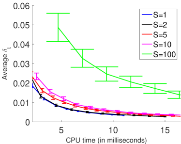
Refer to caption
Refer to caption
Refer to caption
Refer to caption
Figure 6: The convergence of the average relative optimality gap in CBA when using different numbers of comparisons (S𝑆S) in the mini-batch method. First row: h1​(x,ΞΎ)subscriptβ„Ž1π‘₯πœ‰h_{1}(x,\xi); Second row: h2​(x,ΞΎ)subscriptβ„Ž2π‘₯πœ‰h_{2}(x,\xi). First column: ΞΎβˆΌπ’°β€‹[50,150]similar-toπœ‰π’°50150\xi\sim\mathcal{U}[50,150]; Second column: ΞΎβˆΌπ’©β€‹(100,100)similar-toπœ‰π’©100100\xi\sim\mathcal{N}(100,100).

After studying the impact of mini-batch method to CBA, we also show how mini-batch affects SGD and whether the performance of CBA relative to SGD we found in FigureΒ 1 still holds when using different batch sizes. Therefore, we also implement SGD by generating S𝑆S samples of ΞΎπœ‰\xi and using the average of the gradients of hβ„Žh at each sample to perform the stochastic gradient descent step. We also present the convergence of both and CBA and SGD in FigureΒ 7 with S=1,2,5,10,100𝑆12510100S=1,2,5,10,100 in order to compare their performances with different batch sizes. These figures reveal the similar phenomenon as we found in SectionΒ 5.1 that CBA converges more slowly than SGD with the same batch size because CBA uses less information. However, CBA does not require knowing ΞΎπœ‰\xi exactly so that it can be applied in some scenarios where SGD cannot be implemented.
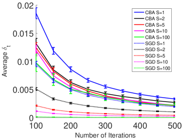
Refer to caption
Refer to caption
Refer to caption
Refer to caption
Figure 7: The convergence of the average relative optimality gap in CBA (solid lines) and SGD (dot lines) when using different batch sizes (S𝑆S) per iteration. First row: h1​(x,ΞΎ)subscriptβ„Ž1π‘₯πœ‰h_{1}(x,\xi); Second row: h2​(x,ΞΎ)subscriptβ„Ž2π‘₯πœ‰h_{2}(x,\xi). First column: ΞΎβˆΌπ’°β€‹[50,150]similar-toπœ‰π’°50150\xi\sim\mathcal{U}[50,150]; Second column: ΞΎβˆΌπ’©β€‹(100,100)similar-toπœ‰π’©100100\xi\sim\mathcal{N}(100,100).

10.2 Categorical Results from Comparison

We conduct numerical experiments to test the performance of the CBA-C (AlgorithmΒ 5) through a comparison with SGD and CBA. We consider the same two objective functions h1subscriptβ„Ž1h_{1} and h2subscriptβ„Ž2h_{2} and the same two distributions of ΞΎπœ‰\xi as in SectionΒ 5.1. The implementation of SGD and CBA, including the choice of Ξ·tsubscriptπœ‚π‘‘\eta_{t}, f+subscript𝑓f_{+} and fβˆ’subscript𝑓f_{-}, is also the same as in SectionΒ 5.1. The number of the categorical results of the comparisons used in CBA-C is chosen to be m=3π‘š3m=3 or m=5π‘š5m=5. To implement CBA-C, we need to specify 2​m2π‘š2m distributions f+isuperscriptsubscript𝑓𝑖f_{+}^{i} and fβˆ’isuperscriptsubscript𝑓𝑖f_{-}^{i} for i=0,1,…,mβˆ’1𝑖01β€¦π‘š1i=0,1,\dots,m-1. When ΞΈi+1<+∞subscriptπœƒπ‘–1\theta_{i+1}<+\infty so that [xtβˆ’ΞΈi+1,xtβˆ’ΞΈi)subscriptπ‘₯𝑑subscriptπœƒπ‘–1subscriptπ‘₯𝑑subscriptπœƒπ‘–[x_{t}-\theta_{i+1},x_{t}-\theta_{i}) and (xt+ΞΈi,xt+ΞΈi+1]subscriptπ‘₯𝑑subscriptπœƒπ‘–subscriptπ‘₯𝑑subscriptπœƒπ‘–1(x_{t}+\theta_{i},x_{t}+\theta_{i+1}] are bounded intervals, we choose fβˆ’isuperscriptsubscript𝑓𝑖f_{-}^{i} and f+isuperscriptsubscript𝑓𝑖f_{+}^{i} to be uniform distributions on the corresponding intervals. For the cases where ΞΈi+1=+∞subscriptπœƒπ‘–1\theta_{i+1}=+\infty (i.e., i=mβˆ’1π‘–π‘š1i=m-1) so that [xtβˆ’ΞΈi+1,xtβˆ’ΞΈi)subscriptπ‘₯𝑑subscriptπœƒπ‘–1subscriptπ‘₯𝑑subscriptπœƒπ‘–[x_{t}-\theta_{i+1},x_{t}-\theta_{i}) and (xt+ΞΈi,xt+ΞΈi+1]subscriptπ‘₯𝑑subscriptπœƒπ‘–subscriptπ‘₯𝑑subscriptπœƒπ‘–1(x_{t}+\theta_{i},x_{t}+\theta_{i+1}] are unbounded in one end, we choose fβˆ’isuperscriptsubscript𝑓𝑖f_{-}^{i} and f+isuperscriptsubscript𝑓𝑖f_{+}^{i} to be exponential distributions as in Example 3.2 with Ξ»+=Ξ»βˆ’=2βˆ’4=0.0625subscriptπœ†subscriptπœ†superscript240.0625\lambda_{+}=\lambda_{-}=2^{-4}=0.0625. For the same reasons given in ExamplesΒ 3.1 and 3.2, the distribution function f+isuperscriptsubscript𝑓𝑖f_{+}^{i} and fβˆ’isuperscriptsubscript𝑓𝑖f_{-}^{i} chosen in this way satisfy (C1’)-(C3’).

Similar to SectionΒ 5.1, in all tests, we start from a random initial point x1βˆΌπ’°β€‹[50,150]similar-tosubscriptπ‘₯1𝒰50150x_{1}\sim\mathcal{U}[50,150] and run each algorithm for T=500𝑇500T=500 iterations and we report the average relative optimality gap Ξ΄t=H​(xΒ―t)βˆ’H​(xβˆ—)H​(xβˆ—)subscript𝛿𝑑𝐻subscriptΒ―π‘₯𝑑𝐻superscriptπ‘₯𝐻superscriptπ‘₯\delta_{t}=\frac{H(\bar{x}_{t})-H(x^{*})}{H(x^{*})} over 200020002000 independent trails for each t𝑑t. The results are reported in Figure 8. The bar at each point represents the standard error of the corresponding Ξ΄tsubscript𝛿𝑑\delta_{t}.

Refer to caption
Refer to caption
Refer to caption
Refer to caption
Figure 8: The convergence of the average relative optimality gap for different algorithms for the four instances. First row: h1​(x,ΞΎ)subscriptβ„Ž1π‘₯πœ‰h_{1}(x,\xi); Second row: h2​(x,ΞΎ)subscriptβ„Ž2π‘₯πœ‰h_{2}(x,\xi). First column: ΞΎβˆΌπ’°β€‹[50,150]similar-toπœ‰π’°50150\xi\sim\mathcal{U}[50,150]; Second column: ΞΎβˆΌπ’©β€‹(100,100)similar-toπœ‰π’©100100\xi\sim\mathcal{N}(100,100).
h1​(x,ΞΎ)subscriptβ„Ž1π‘₯πœ‰h_{1}(x,\xi) h2​(x,ΞΎ)subscriptβ„Ž2π‘₯πœ‰h_{2}(x,\xi)
Algorithm ΞΎβˆΌπ’°β€‹[50,150]similar-toπœ‰π’°50150\xi\sim\mathcal{U}[50,150] ΞΎβˆΌπ’©β€‹(100,100)similar-toπœ‰π’©100100\xi\sim\mathcal{N}(100,100) ΞΎβˆΌπ’°β€‹[50,150]similar-toπœ‰π’°50150\xi\sim\mathcal{U}[50,150] ΞΎβˆΌπ’©β€‹(100,100)similar-toπœ‰π’©100100\xi\sim\mathcal{N}(100,100)
SGD 0.008 0.007 0.010 0.040
CBA 0.011 0.018 0.013 0.049
CBA-C(m=3)π‘š3(m=3) 0.012 0.023 0.023 0.065
CBA-C(m=5)π‘š5(m=5) 0.012 0.026 0.025 0.064
Table 4: The computation time (in seconds) of different algorithms for 500 iterations for the four instances.

From the results shown in Figure 8, we can see that CBA-C converges faster than CBA in these problems. Moreover, the convergence speed of CBA-C is higher for a larger mπ‘šm. This is because the comparison results in CBA-C are categorical instead of binary so that they provide more information about the gap between xπ‘₯x and ΞΎπœ‰\xi which helps to construct a more precision stochastic gradient than CBA. This information becomes more precise as mπ‘šm increases. Also, as shown in TableΒ 4, the computation time of CBA-C for 500 iterations is less than 0.10.10.1 seconds and is similar to CBA.