aainstitutetext: Quantum Gravity and Unified Theory and Theoretical Cosmology Group, Max Planck Institute for Gravitational Physics (Albert Einstein Institute), Am Mu¨¨𝑢\ddot{u}hlenberg 1, 14476 Potsdam-Golm, Germany.bbinstitutetext: Department of Physical Sciences, Indian Institute of Science Education and Research Kolkata, Mohanpur, West Bengal 741246, Indiaccinstitutetext: Ashoka University, Sonepat - 131029, Indiaddinstitutetext: Department of Physics, Birla Institute of Technology, Mesra, Ranchi - 835215, India

Quantum Out-of-Equilibrium Cosmology

Sayantan Choudhury, 111Alternative E-mail: sayanphysicsisi@gmail.com. b    Arkaprava Mukherjee c    Prashali Chauhan d    Sandipan Bhattacherjee sayantan.choudhury@aei.mpg.de,chauhan.prashali@gmail.com, www.farada@gmail.com, arka262016@gmail.com
Abstract

In this work, our prime focus is to study the one to one correspondence between the conduction phenomena in electrical wires with impurity and the scattering events responsible for particle production during stochastic inflation and reheating implemented under a closed quantum mechanical system in early universe cosmology. In this connection, we also present a derivation of quantum corrected version of the Fokker Planck equation without dissipation and its fourth order corrected analytical solution for the probability distribution profile responsible for studying the dynamical features of the particle creation events in the stochastic inflation and reheating stage of the universe. It is explicitly shown from our computation that quantum corrected Fokker Planck equation describe the particle creation phenomena better for Dirac delta type of scatterer. In this connection, we additionally discuss Ito^^𝑜\hat{o}, Stratonovich prescription and the explicit role of finite temperature effective potential for solving the probability distribution profile. Furthermore, we extend our discussion of particle production phenomena to describe the quantum description of randomness involved in the dynamics. We also present computation to derive the expression for the measure of the stochastic non-linearity (randomness or chaos) arising in the stochastic inflation and reheating epoch of the universe, often described by Lyapunov Exponent. Apart from that, we quantify the quantum chaos arising in a closed system by a more strong measure, commonly known as Spectral Form Factor using the principles of Random Matrix Theory (RMT). Additionally, we discuss the role of out of time order correlation function (OTOC) to describe quantum chaos in the present non-equilibrium field theoretic setup and its consequences in early universe cosmology (stochastic inflation and reheating). Finally, for completeness, we also provide a bound on the measure of quantum chaos ( i.e. on Lyapunov Exponent and Spectral Form Factor) arising due to the presence of stochastic non-linear dynamical interactions into the closed quantum system of the early universe in a completely model-independent way.

Keywords:
Cosmology of Theories beyond the SM, Random Matrix Theory, Quantum Chaos, Non-equilibrium statistical field theory, Reheating.

1 Introduction

Quantum fields in an inflationary background Baumann:2009ds ; Baumann:2018muz ; Baumann:2014nda ; Cheung:2007st ; Weinberg:2008hq ; Delacretaz:2016nhw ; Senatore:2016aui ; Delacretaz:2015edn ; LopezNacir:2011kk ; Senatore:2010wk ; Choudhury:2011sq ; Choudhury:2011jt ; Choudhury:2012yh ; Choudhury:2013zna ; Choudhury:2013jya ; Choudhury:2013iaa ; Choudhury:2014sxa ; Choudhury:2014kma ; Choudhury:2014sua ; Choudhury:2014hja ; Choudhury:2015hvr ; Choudhury:2017cos ; Naskar:2017ekm ; Choudhury:2017glj ; Choudhury:2015pqa or during reheating Kofman:1994rk ; Shtanov:1994ce ; Amin:2014eta ; Ozsoy:2015rna ; Giblin:2017qjp ; Kofman:2005yz ; Choudhury:2011rz gives rise to the burst of particle production, which has been extensively studied in ref. Gibbons:1977mu ; SchuTzhold:2013fga ; Winitzki:2005rw . This has been studied to a great extent in the background of the inflationary scenario of the universe in ref.  Birrell:1982ix ; Parker:1968mv ; Fulling:1989nb . Such phenomena has been compared to that of the scattering problem in quantum mechanics with a specific effective potential arising due to the impurity in the conduction wire, which can approximately be solved using the well known WKB technique SchuTzhold:2013fga ; Birrell:1982ix  222In the context of cosmology conformal time dependent effective mass profile exactly mimics the role of impurity potential in electrical conduction wire. Due to such one to one correspondence the time evolution equation (i.e. Klien Gordon equation) of the Fourier modes corresponding to the quantum fluctuation in the context of primordial cosmology can be described in terms of the Schrodinger equation in electrical conduction wire with specific impurity potential. We have investigated this possibility in detail in this paper. Additionally, it is important to note that such time dependent effective mass profiles are also important to study the role of quantum critical quench and eigen state thermalization during the reheating epoch of universe.. It is important to note that such particle production events are completely random (or chaotic) when the evolution is non-adiabatic or tachyonic in nature.
Refer to caption
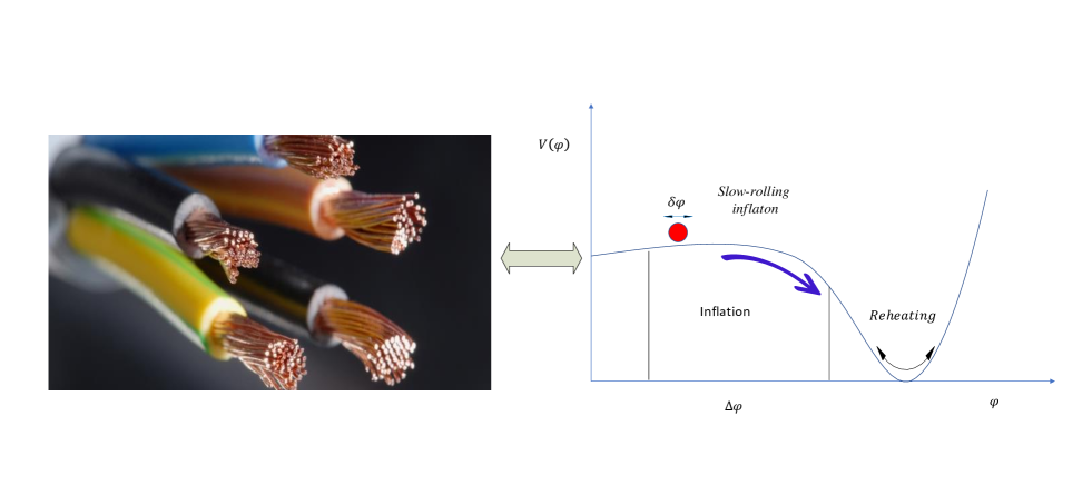
Figure 1: This schematic diagram shows the correspondence between the conduction phenomena in electrical wires with impurity to that of the cosmological random particle-creation events during the non-adiabatic stage of the early universe.

A non-adiabatic change in the time dependent effective mass profiles of the fields (which is actually coming from integrating out the heavy degrees of freedom from the UV complete theory and after path integration finally one gets the time dependent effective coupling parameters between fields) as the background evolution of the fields passes through special points in field space produces these burst of particle creation in (quasi) de Sitter space time. There lies a physical and mathematical equivalence between such cosmological events to that of the stochastic random phenomena occurring in mesoscopic systems where fluctuations in physical quantities play a significant role of producing stochastic randomness in the system under consideration. We also discuss the cosmological systems which have been considered to be rather non-linear and dissipative due to the significant amounts of quantum fluctuations in the effective coupling terms (or in the time dependent effective mass profile) of the interactions between the fields. Important reviews on the non-linear and dissipative effects arising in the context of cosmology were put forward in the refs.  Finelli:2011gd ; Starobinsky:1994bd ; Starobinsky:1986fx ; LopezNacir:2011kk . In this paper we explicitly discuss bout the various non-linear and dissipative effects in cosmological set up that arises in (quasi) de-Sitter space with m2>0superscript𝑚20m^{2}>0, where the term m2superscript𝑚2m^{2} represents the effective mass squared of the created particle in (quasi) de-Sitter background. In this connection it is important to note that, the massless scalar field gets ”thermalize” due to the effective time dependent interaction in the (quasi) de-Sitter background. The cosmological events that we talk about in this paper are identified with those of the particle production stochastic random events. In this paper, we present the dynamical features of inherent chaos (stochastic randomness) in the physical system and its connection with the quantum mechanics in detail. The model is exactly similar to that of ”massless scalar field” interacting with a scatterer in the background which are treated to be the heavy fields and are mainly responsible for cosmological particle production in (qusi) de-Sitter space (seeBirrell:1982ix ). In this context, when the free massless scalar field interacts with the the heavy field in the background space time, it mimics the role of thermalization phenomena of the field which occurs during the epoch of reheating of the universe.
Refer to caption
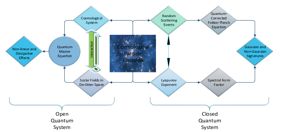
Figure 2: Overview of the computational strategy of the whole paper and how different parts are inter-related.

The specific problem we will discuss here is similar to one presented in ref. Amin:2015ftc . This problem is similar to that of a scattering problem in presence of impurity in quantum mechanics where the Schrödinger equation yields approximate solutions to the wave-function of the particle which encounters a effective impurity potential barrier V(x)𝑉𝑥V(x) of a given strength. The similarity in the following model is drawn between the current carrying electrons responsible for conduction in electrical wires to that of the particle creation in cosmology as a result of the non-adiabatic random events occurring in the early (inflation and reheating) stage of the universe. In this present problem for the sake of simplicity we consider an one dimensional conducting electrical wire, which implies that the current carrying electrons in the electrical wire has only a single propagating degree of freedom. As mentioned earlier, this has been considered to reduce clutter in our computation. But the similar problem can be generalized to more complicated situation 333For an example, one can generalize the same prescription in three space dimensions.. Since, a current carrying wire consists of a large number of impurities, these act like the potential barriers V(x)𝑉𝑥V(x), which are randomly distributed across the wire. Therefore, the motion of the electrons while confronting these scatterers gets hindered due to the presence of these randomly placed scatterers. One of the most important outcome of such an event is known as Anderson Localization as appearing in the context of condensed matter systems. Usually this is characterized by probability density of the localized wave-function:

|ψ(x)|2exp(|x|/ξ),similar-tosuperscript𝜓𝑥2𝑥𝜉\boxed{|\psi(x)|^{2}\sim\exp{\left(|x|/\xi\right)}}~{}~{}, (1)

with ξ𝜉\xi being the localization length of the quantum mechanical wave-function ψ(x)𝜓𝑥\psi(x). This phenomena of Anderson Localization usually occurs due to the interference of the waves scattered from the impurities present in the conduction wire. By formulating cosmological particle production as a random scattering problem, it has been shown in Amin:2015ftc that Anderson localization maps to a problem of estimating exponential particle production, as given by:

|ϕk(τ)|2exp(μkτ),similar-tosuperscriptsubscriptitalic-ϕ𝑘𝜏2subscript𝜇𝑘𝜏\boxed{|\phi_{k}(\tau)|^{2}\sim\exp{\left(\mu_{k}\tau\right)}}~{}~{}, (2)

where μksubscript𝜇𝑘\mu_{k} is the mean particle production rate which is characterized by the conformal time dependent scalar field ϕk(τ)subscriptitalic-ϕ𝑘𝜏\phi_{k}(\tau). A striking similarity has been observed between such scattering problems in conducting wires to that of the burst of particle production in cosmological random events shown in ref. Amin:2015ftc . In such cases, it has been observed that the solving a scattering problem in quantum mechanics using Schrödinger equation is similar to solving a Klein-Gordon equation for a massless scalar field in presence of a conformal time-dependent effective mass squared coupling parameter m2(τ)superscript𝑚2𝜏m^{2}(\tau). In this context the scalar field with time-dependent mass m2(τ)superscript𝑚2𝜏m^{2}(\tau) mimics the role of coupling strength parameter which characterizes the scattering to the massless scalar field in (quasi) de Sitter background. For more details see refs. Bassett:1997gb ; Zanchin:1997gf ; Zanchin:1998fj . Moreover, such stochasticity in a cosmological set up arises due to the stochastic time evolution of Hubble parameter H(t)𝐻𝑡H(t), so that the inflaton (or the field participating in reheating) evolves with time stochastically due to the quantum fluctuations in the FLRW background. In the similar context the role of interacting scalar field has been studied to a great deal in ref. Bassett:1997gb .

In this context,we have presented the the amount by which the quantum mechanical system deviates with respect to the initial conditions. This means that more the value of this exponent, more is the chaos or stochastic randomness in the system under consideration in this paper. This exponent plays a significant role in our scenario as the number of particles produces in a given scattering event per unit time is random in nature. In a system of randomly spaced scatterers chaos emerges out of the random scattering events that an electron encounters while drifting across the wire with some drift velocity v within the conducting wire. The number that quantifies this increase in stochastic randomness or chaos in the system is the Lyapunov Exponent. In refs. Bassett:1997gb ; Amin:2015ftc , particle production phenomena in cosmological non-adiabatic events has been exclusively studied which yields the fact that the particle occupation number depends on Floquet indices μksubscript𝜇𝑘\mu_{k}, which finally control the number of produced particles with the following number density:

nk(τ)=0𝑑kk2exp[2m(τ)μkτ],subscript𝑛𝑘𝜏superscriptsubscript0differential-d𝑘superscript𝑘22𝑚𝜏subscript𝜇𝑘𝜏\displaystyle n_{k}(\tau)=\int_{0}^{\infty}dk~{}k^{2}\exp{\left[2m(\tau)\mu_{k}\tau\right]}~{}~{}, (3)

as well as the variances in the field fluctuation. The quantum fluctuations in the inflationary state of the universe results in the randomization of these bursts of particle production. The number density has been a random variable which is rendered stochastic due to the scattering events in the context of early universe cosmology. Our main objective in this paper to quantify this characteristic number for the massless scalar field having a conformal time-dependent mass coupling with it. One of the prime reasons for finding a signature of chaos in such a system is the well known thermalization phenomena, which means that the FLRW background which embeds the massless scalar field into it is being thermalized by the massive field in interaction with the FLRW set up, which constantly being giving rise to a burst of particle production in the context of early universe cosmology. The scalar fields that we considering in our paper are said to be massive or heavy fields (mH𝑚𝐻m\geq H) which mimics the role of the scatterers in the Schrödinger problem in quantum mechanics where the strength of the effective potential or the scatterer is given by the probability distribution function of the effective potential function. We draw a picturesque landscape by considering three distinct mass profiles:

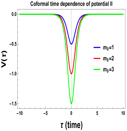
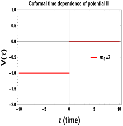
m2(τ)={m022[1tanh(ρτ)],Profile  I m02sech2(ρτ),Profile  II m02Θ(τ).Profile  III ,superscript𝑚2𝜏casessuperscriptsubscript𝑚022delimited-[]1𝜌𝜏Profile  I missing-subexpressionsuperscriptsubscript𝑚02superscriptsech2𝜌𝜏Profile  II missing-subexpressionsuperscriptsubscript𝑚02Θ𝜏Profile  III missing-subexpressionmissing-subexpressionmissing-subexpression\displaystyle\begin{array}[]{lll}\displaystyle m^{2}(\tau)=\left\{\begin{array}[]{lll}\displaystyle\frac{m_{0}^{2}}{2}\left[1-\tanh(\rho\tau)\right]\,,{}{}{}{}{}{}{}{}{}{}{}{}&\mbox{\small{\color[rgb]{1,0,0}\bf{Profile~{} I }}}\\ \displaystyle m_{0}^{2}~{}{\rm sech}^{2}(\rho\tau)\,,{}{}{}{}{}{}{}{}{}{}{}{}&\mbox{\small{\color[rgb]{1,0,0}\bf{Profile~{} II }}}\\ \displaystyle m_{0}^{2}~{}\Theta(-\tau).{}{}{}{}{}{}{}{}{}{}{}{}&\mbox{\small{\color[rgb]{1,0,0}\bf{Profile~{} III }}}\end{array}\right.\end{array}, (8)

which exactly mimics the role of cosmological scatterers in early universe. We thereby investigate the momentum scale dependent behaviour of the Lyapunov exponent. In this context, the incoming momenta of the mode functions of the quantized massless scalar field having random interactions with the scatterer. In the following class of model, the Bogoliubov coefficients arise due to the interaction between massless scalar field with the heavy field. These Bogoliubov coefficients gives the information about the transmission coefficient viz.a.viz in similar problem to that of a scattering problem in quantum mechanics, that we solve using the well known WKB approximation technique 444To find approximate solution of the Schrödinger equation (or in other words the Klein-Gordon field equation) in presence of an arbitrary impurity effective potential, (or the conformal time dependent mass coupling parameter) WKB approximation method plays crucial role Choudhury:2016cso ; Choudhury:2016pfr .. These WKB solutions are extremely useful as it tell us the dynamical feature of the particle production in cosmological scattering events.

In continuation with this, we discuss about the epoch of reheating which occurs after the end of inflationary stage of the universe which finally results in the stochastic random burst of particle production. The dynamics of these stochastic random bursts of particle production can be well understood by using a Fokker-Planck equation, which gives us a statistical interpretation of the number density of particles created per scattering event. Since, the number of particles created in a given non-adiabatic event is not discrete in nature but rather its random, which means that there must be a probability distribution function associated with the particle number. The various dynamical features of this type of probability distribution and its physical consequences has been studied in ref. Amin:2015ftc . It has been phenomenologically proposed in ref. Amin:2015ftc that such probability density function would necessarily is Gaussian one. The occupation number of the produced particles, nksubscript𝑛𝑘n_{k}, executes a drifting Brownian motion and a Fokker-Planck (FP) equation that evolves the probability distribution, P(nk;τ)𝑃subscript𝑛𝑘𝜏P(n_{k};\tau), emerging out of this Brownian motion has been studied in ref. Amin:2015ftc . We further compute the analytical expressions for the mean, variance and other higher order moments which are commonly known as, skewness and kurtosis and such additional statistical higher order moments are very useful to study the exact mathematical form and asymptotic limits of the probability distribution function. The evolution of mean, variance, skewness and kurtosis finally gives a coarse-grained analysis of the Fokker-Planck dynamics to more corrected orders of magnitude in quantum regime. We show in this paper explicitly that though Gaussianity is an inherent part of the probability density function, but the consideration of the higher order moments in the Fokker-Planck equation tells us that the density function may not be a Gaussian one but with some higher-order corrections entailed into it due to the quantum mechanical origin. Therefore, to a greater extent we extend the more corrected quantum version of the Fokker-Planck equation used to describe the dynamics of the probability distribution function used in ref. Amin:2015ftc that tells us the dynamics of the bursts of particle production in these random scattering events. The more quantum corrected version tells us that the probability amplitude of the particle production in the scattering events is more than a Log normal distribution. The distribution profile of the probability distribution function depends largely on the profile of the scatterer, i.e., the effective potential V(x)𝑉𝑥V(x) in the Schrödinger-like equation. While calculating the Fokker-Planck dynamics we observe that the skewness gives us a clue about the rate at which the particle production occurs meaning that longer the trailing part of the profile more is the number density of particles in the scattering event for a given time in the frame of the observer, whereas, kurtosis tells us the width of the probability distribution function which is essentially the amplitude with which the particle production phenomena occurs, which more suggestively tells us about the standard deviation of the density function from Gaussianity. This may be a signature of non-Gaussianity that arises in various models in early universe cosmology.

In this connection it is important to note that, such stochastic approaches to the early universe scenario have been studied in details in Linde:2002yd ; Koks:1997rk , where the authors give an account of how chaos arises in the context of eternal inflation. As any rapidly oscillating classical field looses its energy by creating pairs of elementary particles, these particles interact with each other and comes to a state of showing thermal behaviour at some temperature T𝑇T. This implies that we must eliminate the necessary assumption of the universe being in thermal equilibrium. This means that the inflating universe is rather thermal in the sense that the particle creation events that occurs during the quantum fluctuation in the randomly distributed scalar fields ϕitalic-ϕ\phi which results in a chaotic model of the inflationary scenario of the universe thereby leading to a generation of stochastic idea of the particle creation events during the thermalization of the quantum states of the field randomly distributed over the space-time. These particle creation events are more phenomenologically associated with one of the fundamental ideas in out-of-equilibrium statistical mechanics known as Fokker-Planck equation which gives the rate of the particle production during theses random events in stochastically emerging space-time along with the distribution function that this rate charts out. In ref. Amin:2015ftc , such a phenomenon of particle creation events by the randomly spaced scatterers in due context of cosmology has been shown where the the statistics of the produced particles as a function of time which is the probability distribution function P(nk,τ)𝑃subscript𝑛𝑘𝜏P(n_{k},\tau) has been predicted to be following a Log-Normal distribution. The entire process have been carried out with the delta-scatterers which are localized in space-time.

Following ref. Amin:2015ftc , in this paper we give a more improved quantum corrected version of the same approach to the probability density function of the particle production events and our prediction from the results show that the higher order quantum correction terms being included into the Fokker-planck equation introduces an approximation to the theory. This tells us that the number of particles produced in a given non-adiabatic event during the reheating stage of the universe is quantized, which would mean that the rate of particle production in a given event gives rise to a discrete set of occupation number nksubscript𝑛𝑘n_{k}. Furthermore, the quantum corrected terms obtained by deriving the Fokker-Planck equation takes the general form, which is linear in nksubscript𝑛𝑘n_{k} being the first order in τ𝜏\tau. Using this information we calculate further the leading order, second and third order terms in the Fokker-Planck equation. Hence, we derive the analytic expression of the quantum corrected version of Fokker-Planck equation. We also calculate the various higher moments in order to get an overview of the nature of the solution of the quantum corrected Fokker-Planck equation which are - standard deviation, skewness and kurtosis which gives the hint of how the probability density function deviates from its Gaussian nature when the higher order quantum corrections are taken into account in the computation. This in turn may will be another indirect signature of the primordial non-Gaussianity in cosmology other than obtaining the signatures provided by the 3-point functions from scalar fluctuations.

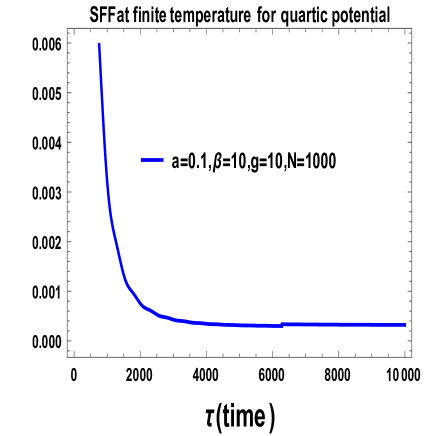
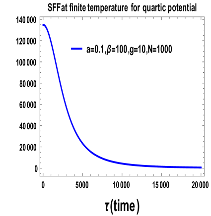
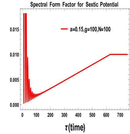
Apart from that, we discuss about spectral form factor (SFF), which measures the random distribution of eigen values of the energy hamiltonian of a chaotic system. For this computation of SFF we use the principles of random matrix theory (RMT) in this paper. In the present context an upper bound on SFF denotes the saturation of eigen value distribution hence supports the ref. Maldacena:2015waa for quantum chaotic system. Within the framework of quantum physics, chaotic systems can be characterized using only some additional constraints. This theoretical approach is discussed in refs. Dyson:1962es ; Dyson:1970tza ; Dyson:1962a ; Dyson:II ; Dyson:IV and the authors use the theory of random matrices to characterize quantum mechanical system. In this method, any arbitrarily complicated many-body Hamiltonian can be replaced by matrix of random numbers drawn from a Gaussian statistical ensemble. This random matrix approach towards quantum mechanics help to characterize and understand the underlying features of the chaotic random system. After studying the behaviour of SFF with time one can further comment that whether it is valid for a cosmological particle production event (semi-classical) or not. For our purpose we discuss generalized version of SFF for different even order polynomial structure of random potential and then extend that result to describe the cosmological particle production events Maldacena:2016hyu ; Garcia-Garcia:2016mno . For any random potential we can use this method of SFF and we can deal with scatterer of any arbitrary type. For any such scatterer we can get a bound on randomness in the chaotic system characterised by SFF. Also using specific transfer matrix for different conformal time dependent effective mass profiles which are precisely known in this paper, we can finally compute Lyapunov exponent which also measure stochastic randomness.

Also it is important to note that in ref. Amin:2015ftc , the scatterers were considered to be some localized potential functions in space-time. On the contrary the choice of our specific time dependent mass profiles mimics the role of thermalized fields or effective potential functions, which are playing the role of scatterers in this context. We see that the choice of these time dependent mass profiles leads to particle production which is chaotic in nature and therefore, to determine the rise of chaos in such a system we quantify as well as analyse chaos by a well known quantities known as the , Lyapunov exponentMandal:2015kxi and Spectral Form Factor (SFF) Gaikwad:2017odv . Here fusing the principles of random matrix theory (RMT) we provide a generalized bound on randomness (or stochasticity) for any general random scatterer whose potential can be expressed in terms of an even polynomial. More precisely, we provide a possible method to compute the degree of randomness in a chaotic system and from that one can check the bound on chaos.

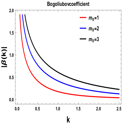
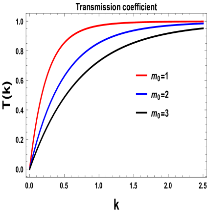
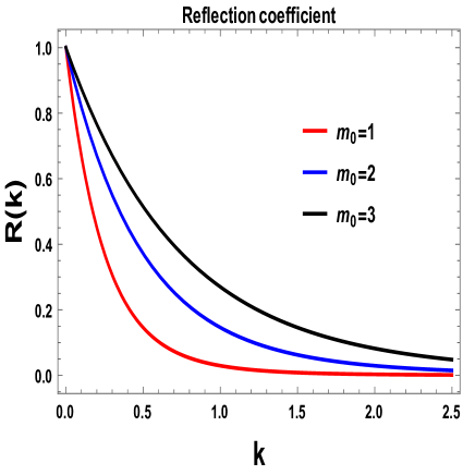
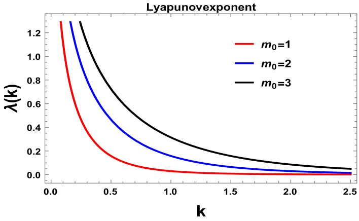
The plan of the paper is as follows - In section 2 we discuss about the model which is responsible for the quantum description of chaos during the cosmological particle production and have similarities with the quantum mechanical problem of electrical conducting wire with impurities. In section 3, we have presented the analytical expressions for the Bogoliubov coefficients, transmisson and reflection coefficients, Lyapunov exponent, conductance, and resistance for different time dependent mass profile. We have discussed the correspondence between In section 5 the specific role of Spectral Form Factor (SFF) to quantify chaos in the context of particle production rate is discussed. In section 6 the particle production event with quantum corrected Fokker-Planck equation is discussed by taking contribution upto fourth order and also different higher order moments from the quantum corrected probability density function are explicitly computed. Finally, in section 7 we conclude with the future prospect and physical impacts of our work.

Additionally it is important to note that, throughout this paper, we use natural system of units, =c=1Planck-constant-over-2-pi𝑐1\hbar=c=1.

2 Modelling randomness in cosmology

The background model which we consider in this section to quantify quantum chaos in cosmology consists of a massless scalar field interacting with coupled with a background scalar field with conformal time dependent mass profile which in principle have heavier or comparable to the Hubble scale (mH𝑚𝐻m\geq H) Arkani-Hamed:2015bza ; Maldacena:2015bha ; Choudhury:2016cso . It is important to note that such heavy mass profiles play significant role in finding various cosmological correlation functions and also can be treated as an additional probe to break the degeneracy between various models of inflation from the perspective of implementing cosmological perturbation theory in (quasi) de Sitter background. We know that in usual set up of primordial cosmological perturbation such heavy fields are not appearing in the low energy effective field theory action. For that case in the simplest situation we actually start with an one field set up where the kinetic term is canonical in nature and the field is minimally coupled with the background gravity which is treated to be classical usually. Also such field has an effective structure of the interaction potential which play crucial role to study the time dynamics in FLRW cosmological background. Here specifically the field is treated to be massless compared to the Hubble scale (m<<Hmuch-less-than𝑚𝐻m<<H). However, this is not the complete story yet. To explain this let us start with a Ultra Violet (UV) complete set up of quantum field theory (QFT) such as string theory in higher dimensions. There are various examples of string theory from which one can start the computation, which are - Type II A, Type II B, Heterotic, M - theory etc. Also the low energy extension of such theories (supergravity) are also useful for the computation in the context of cosmology. Here it is important to note such all such theories contain massive (m>>Hmuch-greater-than𝑚𝐻m>>H), intermediate mass (mH𝑚𝐻m\approx H) and massless (m<<Hmuch-less-than𝑚𝐻m<<H) fields in the matter multiplet. To write down an effective field theory (EFT) one need to integrate out all such heavy degrees of freedom from the UV complete version of the action 555Important notes:
       Here we note the following points which are very useful to study the consequences from EFT set up: 1. In this context, one can construct an EFT by utilizing the underlying symmetries appearing in the field theoretic set up. In such a generalized description where EFT is constructed by following the top down approach, we really don’t care about the exact UV completion of the parent theory i.e. detailed quantum field theory origin at high energy scale of such effective constructions are not important in this case. See ref. Cheung:2007st ; Choudhury:2017glj for more technical details. 2. In a more generalized prescription of EFT one can construct the set up which requires to correctly account for all relevant self interactions of adiabatic modes around and after the cosmological horizon crossing. Specifically the adiabatic mode contains all types of EFT relevant operators, including transient reductions in the effective sound speed cSsubscript𝑐𝑆c_{S} each time the background field undertakes non-geodesic motion in background target space. In an EFT framework with single field setting, where heavy directions are such that the mass of the field under consideration is heavy compared to the Hubble scale i.e. m>>Hmuch-greater-than𝑚𝐻m>>H, one gets transient drops in the effective sound speed cSsubscript𝑐𝑆c_{S} during slow roll if the potential is such that the field traverses a bend even if the parent theory consists of canonically normalized scalar fields. So for general consideration one can allow many more possibilities without following any restriction to time dependent mass profile. However, these three specific types of time dependent mass profiles are very popular in the context of the study of quantum critical quench in a analytical fashion. We have considered these profiles particularly as our future objective is to apply the idea of quantum quench in the context of De Sitter space to quantify randomness during reheating phase. It is important to note that, using a simple field redefinition at the level of quantum fluctuation to the Mukhanov-Sasaki variable which results in a time dependent mass for the rescaled variable appearing with additional contributions of the mathematical form, cS˙/cSSHsimilar-to˙subscript𝑐𝑆subscript𝑐𝑆𝑆𝐻\dot{c_{S}}/c_{S}\sim SH. Here S=cS˙/HcS𝑆˙subscript𝑐𝑆𝐻subscript𝑐𝑆S=\dot{c_{S}}/Hc_{S} is the associated slow roll parameter with the effective time dependent sound speed cSsubscript𝑐𝑆c_{S} and H𝐻H is the Hubble parameter and it is associated with the changes in the radius of curvature of the inflaton trajectory. In this case the effective sound speed is given by, cS21+4ϕ˙2/κ2M2subscriptsuperscript𝑐2𝑆14superscript˙italic-ϕ2superscript𝜅2superscript𝑀2c^{-2}_{S}\equiv 1+4\dot{\phi}^{2}/\kappa^{2}M^{2}, where κ𝜅\kappa is the radius of curvature of the background inflaton (ϕitalic-ϕ\phi) trajectory and M𝑀M is the effective cut-off scale of the EFT at high energy (UV) regime. Equivalently, it refers to the degree to which effective sound speed cSsubscript𝑐𝑆c_{S} is reduced, which actually quantify the distance from the adiabatic minimum of the potential in the background inflaton trajectory is forced by its evolution. Each of these possibilities has different applications in the low energy limiting region of EFT. When the effective sound speed cS<<1much-less-thansubscript𝑐𝑆1c_{S}<<1 and c˙S0similar-tosubscript˙𝑐𝑆0\dot{c}_{S}\sim 0 is fixed over few e-folds of expansion then it is extremely difficult to maintain a meaningful derivative expansion without considering other types of special symmetries appearing in the set up. However, as mentioned earlier, within certain limits one can consider an adiabatic region where the effective sound speed cS<<1much-less-thansubscript𝑐𝑆1c_{S}<<1 and c˙ScSHsimilar-tosubscript˙𝑐𝑆subscript𝑐𝑆𝐻\dot{c}_{S}\sim c_{S}H and S=cS˙/HcS1𝑆˙subscript𝑐𝑆𝐻subscript𝑐𝑆similar-to1S=\dot{c_{S}}/Hc_{S}\sim 1 is fixed over a very small e-fold of expansion and this in turn generate all possible consistent transient strong coupling parameters without violating perturbative uniterity and these terms are explicitly appearing in the derivative expansion in the EFT. Consequently, the nature of these two types of features in the effective sound speed cSsubscript𝑐𝑆c_{S} give rise to distinctive contributions to the physical observables studied in the EFT set up. The positive detection of these physical observables in different experiments allow to extract the underlying non-trivial physics from the EFT set up. In the technical ground the adiabatic mode is identified with the Goldstone boson, which is appearing due to spontaneously broken time translational symmetry prior to the path integration of the heavy fields. In this context, the invariance of the parent theory completely fixes the entire non-perturbative structure of all possible Wilsonian EFT operators and the associated coupling parameters can be expressed entirely by the effective sound speed cSsubscript𝑐𝑆c_{S} of adiabatic perturbations, where the adiabaticity conditions cS<<1much-less-thansubscript𝑐𝑆1c_{S}<<1 and c˙ScSHsimilar-tosubscript˙𝑐𝑆subscript𝑐𝑆𝐻\dot{c}_{S}\sim c_{S}H are respected. In principle, cSsubscript𝑐𝑆c_{S} can be computed in terms of the parameters of the parent theory. Thus the additional contributions appearing in the adiabatic limit cS<<1much-less-thansubscript𝑐𝑆1c_{S}<<1 and c˙ScSHsimilar-tosubscript˙𝑐𝑆subscript𝑐𝑆𝐻\dot{c}_{S}\sim c_{S}H directly justifies the validity of our treatment in this paper. For further technical details of this EFT set up see ref. Achucarro:2010da ; Achucarro:2012sm ; Chluba:2015bqa .
. After doing dimensional reduction along with applying various compactification techniques one can derive various types of UV complete effective field theories at cosmological scale where the effective couplings of various relevant and irrelevant Wilsonian operators have time dependent profile in FLRW background and in such a case from the relevant quadratic operator one can also get the time dependent effective mass which is in general heavy (mH𝑚𝐻m\geq H). It is further important to mention here that, such heavy fields can give rise to non vanishing one point function for scalar (curvature) perturbation in cosmology, which carries the signature of Bell’s inequality violation in primordial universe Maldacena:2015bha ; Choudhury:2016cso ; Kanno:2017dci ; Kanno:2016qcc ; Kanno:2014bma ; Kanno:2014ifa ; Kanno:2014lma . Also it is important to note that such Bell violating set up can be explained using the theory of quantum entanglement in (quasi) de Sitter background and can give rise to non-vanishing quantum information theoretic measure i.e. Von Neumann entropy, Re´´𝑒\acute{e}nyi entropy, quantum discord, logarithmic entangled negativity Choudhury:2017bou ; Choudhury:2017qyl ; Maldacena:2012xp ; Albrecht:2018prr etc. Additionally, one can get correct expression for two point function and also the three point function from scalar (curvature) perturbation, which will show significant effect in estimating primordial non-Gaussianity from single field models of inflation. Apart from this one can consider a simplest situation in four space-time dimensions where the cosmological dynamics is explained in terms of two interacting scalar fields. The light field (m<<Hmuch-less-than𝑚𝐻m<<H) is participating in inflation and the other heavy field (m>>Hmuch-greater-than𝑚𝐻m>>H) is participating to explain the dynamics of reheating. If we path integrate out the reheating degrees of freedom then we get an effective field theory of inflation which is exactly same as we have explained earlier. But here one can consider the other possibility as well in which one can path integrate out the light inflaton degrees of freedom and write down an effective field theory to describe reheating in terms of the heavy fields (mH𝑚𝐻m\geq H). In such a description this reheating field have mass and in the effective field theory description one can write down some time dependent coupling in terms of the integrated inflaton degrees of freedom and the mass of the reheating field appearing in the coefficient of the relevant quadratic operator. In this description such time dependent coupling is treated to be the time dependent effective mass parameter profile which is considered in the present discussion. So it is evident from this discussion that using both the effective field theory of inflation and reheating one can actually explain the origin of such time dependent effective mass profiles in four dimensions. However, in this paper since our objective is to study the cosmological particle production phenomena, we will mostly focus on the reheating epoch of the universe.

The dynamics of this fluctuating scalar field 666Here it is important to note that, for inflation this scalar field is actually massless and in the effective field theory description one can construct the time dependent effective mass profile. On the other hand, in the context of reheating the scalar field is massive and in the effective field theory description one can construct time dependent effective mass in terms of the original mass of the reheating field and other degrees of freedom which are integrated out from the original theory. in FLRW cosmological background with a time-dependent coupling obeys the following Klein-Gordon equation 777Here we have assumed that the effective sound speed parameter, cS=1subscript𝑐𝑆1c_{S}=1, which indirectly implies the fact that for background time evolution we are considering a single scalar field with canonical kinetic term minimally coupled to the gravity. Effective mass of the scalar field is m(τ)𝑚𝜏m(\tau), which has time dependent profile. However, one can generalize this prescription for any general non-canonical single field (i.e.P(X,ϕ)𝑃𝑋italic-ϕP(X,\phi) theory) theoretic framework where the effective sound speed parameter cS1subscript𝑐𝑆1c_{S}\neq 1. :

[d2dτ2+(k2+m2(τ))]ϕk(τ)=0,delimited-[]superscript𝑑2𝑑superscript𝜏2superscript𝑘2superscript𝑚2𝜏subscriptitalic-ϕ𝑘𝜏0\boxed{\left[\frac{d^{2}}{d\tau^{2}}+\left(k^{2}+m^{2}(\tau)\right)\right]\phi_{k}(\tau)=0}~{}~{}, (9)

where m2(τ)superscript𝑚2𝜏{m^{2}(\tau)} is the time dependent mass of the scalar field with which is originating from the effective field theory (EFT) of massless scalar field coupled with other heavy degrees of freedom by following the two possibilities:

  1. 1.

    In EFT time dependent couplings are appearing after path integrating out the massive degrees of freedom. This prescription is usually used to construct a most generic EFT of inflation.

  2. 2.

    In EFT time dependent couplings are appearing after path integrating out the massless degrees of freedom. This prescription is usually used to construct a most generic EFT of reheating.

Here ϕk(τ)subscriptitalic-ϕ𝑘𝜏\phi_{k}(\tau) is the associated Fourier mode of the fluctuating scalar field with momentum k𝑘k, where it plays the role of wave number in the present context.

In this paper, our prime objective is to find a precise equivalence between the dynamics of this scalar field resulting in stochastic particle production in cosmological events during reheating and the similarity with the dynamics of the electron transport in conduction wires. To establish this equivalence we start with the fact that the above mentioned Klein-Gordon equation for the fluctuating scalar field in (quasi) de Sitter background shows a striking similarity with the time-independent one dimensional Schrödinger equation appearing in the context of quantum mechanical system which describes the space evolution of electron inside a wire in presence of impurity as given by:

[d2dx2+EV(x)]ψ(x)=0,delimited-[]superscript𝑑2𝑑superscript𝑥2𝐸𝑉𝑥𝜓𝑥0\displaystyle\left[\frac{d^{2}}{dx^{2}}+E-V(x)\right]\psi(x)=0, (10)
Scattering in conduction wire Cosmological particle creation
Symbol Physical interpretation Symbol Physical interpretation
x Distance τ𝜏\tau Conformal time
V(x) Potential -m2(τ)superscript𝑚2𝜏m^{2}(\tau) Time Dependent mass parameter
Ψ(x)Ψ𝑥\Psi(x) Wave Function ϕk(τ)subscriptitalic-ϕ𝑘𝜏\phi_{k}(\tau) Mode function in Fourier space
Nssubscript𝑁𝑠N_{s} No. of Scatterers Nssubscript𝑁𝑠N_{s} No. of non-adiabatic events
ΔΔ\Deltax Distance between scatterers ΔτΔ𝜏\Delta\tau Time between non-adiabatic events
ξ𝜉\xi Localization length μksubscript𝜇𝑘\mu_{k} Mean particle production rate
ρ(x)𝜌𝑥\rho(x) Resistance nk(τ)subscript𝑛𝑘𝜏n_{k}(\tau) Particle occupation number
E𝐸E Energy eigen value k2superscript𝑘2k^{2} Wave number of Fourier modes
Ncsubscript𝑁𝑐N_{c} Number of channels Nfsubscript𝑁𝑓N_{f} Number of fields
Table 1: A brief overview of the connection between the scattering problem in quantum mechanics to that of cosmological particle creation events.

where, V(x)𝑉𝑥V(x) corresponds to the time-dependent potential which is appearing as an outcome of impurity in the electrical wire and plays the similar role of negative of the square of time-dependent mass profile as appearing in the context of cosmology i.e. m2(τ)superscript𝑚2𝜏-m^{2}(\tau). Also E𝐸E represents the energy eigen value which mimics the role of the wave number squared i.e. k2superscript𝑘2k^{2}. Finally, ψ(x)𝜓𝑥\psi(x) represents the wave function of the quantum mechanical system under consideration which is similar to the Fourier modes of the time dependent fluctuating scalar field in the context of cosmology i.e. ϕk(τ)subscriptitalic-ϕ𝑘𝜏\phi_{k}(\tau). The above set up can be re-expressed in terms of solving a transfer matrix problem since the scatterers can be thought as potential profiles in Schrödinger problem in quantum mechanics with the incoming and outgoing modes of the scalar field related to each other with the Bogoliubov coefficients. A complete overview of the connection between the variables that quantify the scattering problem in the context of quantum mechanics to the one in the cosmological particle production problem has been shown in table (1).

It is very well known fact that the conductance of the electrical wire is related to the transmission probability of electrons across the wire and this can be obtained by explicitly solving the time-independent Schrödinger equation (see Eq (11)) in the presence of the impurities. Before going to the further details of the computation here we begin by reviewing the scattering problem by a single impurity localized at the position x=xj𝑥subscript𝑥𝑗x=x_{j}. To the left (L) and the right (R) of the impurity potential, the wave-function can be written as a linear combination of right-propagating waves (exp(ikx)𝑖𝑘𝑥\exp\left(ikx\right)) and the left-propagating waves (exp(ikx)𝑖𝑘𝑥\exp\left(-ikx\right)) as:

ψΔ(x)=βΔexp(ikx)+αΔexp(ikx)whereΔ=L,R,formulae-sequencesubscript𝜓Δ𝑥subscript𝛽Δ𝑖𝑘𝑥subscript𝛼Δ𝑖𝑘𝑥whereΔ𝐿𝑅\displaystyle\psi_{\Delta}(x)=\beta_{\Delta}\exp\left(ikx\right)+\alpha_{\Delta}\exp\left(-ikx\right)~{}~{}~{}~{}~{}~{}~{}~{}{\rm where}~{}\Delta=L,R, (11)

This is essentially a scattering problem in the context of quantum mechanics in which the impurities act as interaction potentials or scatterers across which the electrons get transmitted within the conduction wire. The map between the Bogoliubov coefficients (βR,αR)subscript𝛽𝑅subscript𝛼𝑅(\beta_{R},\alpha_{R}) from the right (R) side and the Bogoliubov coefficients (βL,αL)subscript𝛽𝐿subscript𝛼𝐿(\beta_{L},\alpha_{L}) from the left (L) side can be expressed in terms of the following Bogoliubov transformation equation as:

R=jL,subscript𝑅subscript𝑗subscript𝐿\displaystyle{\cal B}_{R}={\cal M}_{j}~{}{\cal B}_{L}, (12)

where we define:

Δ=(βΔαΔ)whereΔ=L,R,formulae-sequencesubscriptΔmatrixsubscript𝛽Δsubscript𝛼ΔwhereΔ𝐿𝑅\displaystyle{\cal B}_{\Delta}=\begin{pmatrix}\beta_{\Delta}\\ \alpha_{\Delta}\end{pmatrix}~{}~{}~{}~{}~{}~{}~{}~{}~{}{\rm where}~{}\Delta=L,R, (13)

and in this context the transfer matrix for the j𝑗j-th scatterer jsubscript𝑗{\cal M}_{j} is given by the following expression:

j=(1tjrjtjrjtj1tj),subscript𝑗matrix1subscriptsuperscript𝑡𝑗subscriptsuperscript𝑟𝑗subscriptsuperscript𝑡𝑗subscript𝑟𝑗subscript𝑡𝑗1subscript𝑡𝑗\displaystyle{\cal M}_{j}=\large\begin{pmatrix}\large~{}~{}\frac{1}{t^{*}_{j}}~{}~{}~{}~{}&\frac{-r^{*}_{j}}{t^{*}_{j}}~{}~{}\\ ~{}~{}\frac{-r_{j}}{t_{j}}~{}~{}~{}~{}&\frac{1}{t_{j}}~{}~{}\end{pmatrix}, (14)

which is essentially an unitary matrix related the incoming and the outgoing wave functions and their normalization coefficients.

Ultimately, using this methodology our objective is to connect several impurities together. This is particularly very easy to describe in terms of the transfer matrix approach, since the total transfer matrix across Nssubscript𝑁𝑠N_{s} number of scatterers is simply given by the simple matrix multiplication of the individual transfer matrices as given by the following expression:

(Ns)=j=1Nsj=NsNs1321.subscript𝑁𝑠subscriptsuperscriptproductsubscript𝑁𝑠𝑗1subscript𝑗tensor-producttensor-productsubscriptsubscript𝑁𝑠subscriptsubscript𝑁𝑠1subscript3subscript2subscript1\displaystyle{\cal M}\equiv{\cal M}(N_{s})=\prod^{N_{s}}_{j=1}{\cal M}_{j}={\cal M}_{N_{s}}\otimes{\cal M}_{N_{s}-1}\otimes......\otimes{\cal M}_{3}\otimes{\cal M}_{2}\otimes{\cal M}_{1}. (15)

For our choice of convenience of symbols we will drop the term Nssubscript𝑁𝑠N_{s} for the Nssubscript𝑁𝑠N_{s} number of scatterers and hence we will be considering this to be equal to {\cal M}.

Refer to caption
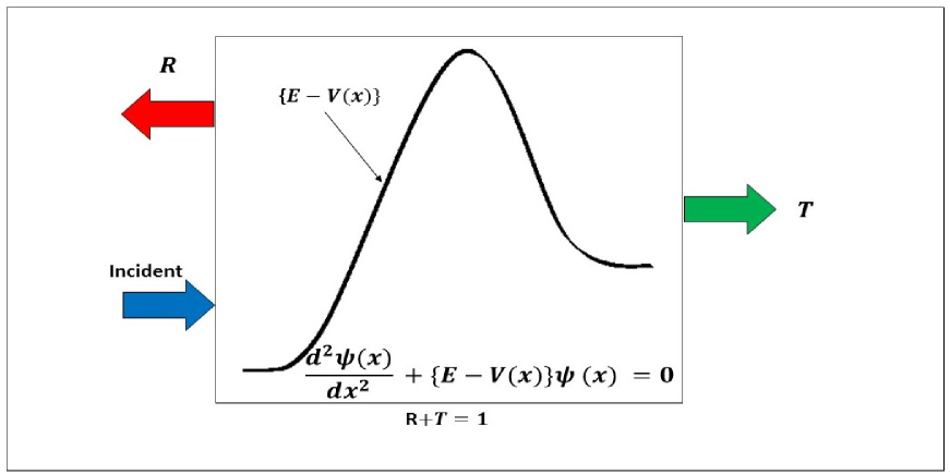
Figure 3: This diagram shows that incoming wave of electron encounter a scatterer and it partially passes through it with T(transmisson probability) and partially reflected back with R(reflection probability).

In Fig:3 we show the electron(wave) encounter a potential(impurity or scatterer).It transmit and reflect through it.From simalirty of Klein-Gordon equation and the time-independent one dimensional Schrödinger equation we calculate R and T for particle production event. Further, let us consider the simplest possibility of having two (Ns=2subscript𝑁𝑠2N_{s}=2) scatterers across which the transmission probability can be written as:

T=T1T2|1R1R2eiθ|2,𝑇subscript𝑇1subscript𝑇2superscript1subscript𝑅1subscript𝑅2superscript𝑒𝑖𝜃2\displaystyle T=\frac{T_{1}T_{2}}{|1-\sqrt{R_{1}R_{2}}e^{i\theta}|^{2}}, (16)

where the transmission and reflection coefficients for the jth𝑗𝑡j-th scatterer can be expressed as:

Tj=tjtj,Rj=rjrjj=1,2.formulae-sequencesubscript𝑇𝑗subscriptsuperscript𝑡𝑗subscript𝑡𝑗formulae-sequencesubscript𝑅𝑗subscriptsuperscript𝑟𝑗subscript𝑟𝑗for-all𝑗12\displaystyle T_{j}=t^{*}_{j}t_{j},~{}~{}~{}R_{j}=r^{*}_{j}r_{j}~{}~{}~{}~{}~{}\forall j=1,2. (17)

and additionally eiθsuperscript𝑒𝑖𝜃e^{i\theta} is the overall phase factor which describes the shift in phase between the reflecting waves across the scatterers due to the presence of impurities. If the distance between the two impurities is random in nature and uniformly distributed over a region with the assumption, kΔx>>1much-greater-than𝑘Δ𝑥1k\Delta x>>1 (where Δx=x2x1Δ𝑥subscript𝑥2subscript𝑥1\Delta x=x_{2}-x_{1} is the distance between the scatterers), then the phase θ𝜃\theta is also uniformly distributed over the interval 0<θ<2π0𝜃2𝜋0<\theta<2\pi. Using this fact explicitly we take logarithm on both sides of the above equation and further doing average over the phase within the interval 0<θ<2π0𝜃2𝜋0<\theta<2\pi we finally get 888Following this discussion, one can generalize this statement for Nssubscript𝑁𝑠N_{s} number of scatterers as: logTθ=log(j=1NsTj)=j=1NslogTj.subscriptdelimited-⟨⟩𝑇𝜃subscriptsuperscriptproductsubscript𝑁𝑠𝑗1subscript𝑇𝑗subscriptsuperscriptsubscript𝑁𝑠𝑗1subscript𝑇𝑗\displaystyle\langle\log{T}\rangle_{\theta}=\log\left(\prod^{N_{s}}_{j=1}T_{j}\right)=\sum^{N_{s}}_{j=1}\log T_{j}. (18) :

logTθ=logT1+logT2+2log|1R1R2eiθ|θ=0=log(j=12Tj)=j=12logTjsubscriptdelimited-⟨⟩𝑇𝜃subscript𝑇1subscript𝑇2subscript2subscriptdelimited-⟨⟩1subscript𝑅1subscript𝑅2superscript𝑒𝑖𝜃𝜃absent0subscriptsuperscriptproduct2𝑗1subscript𝑇𝑗subscriptsuperscript2𝑗1subscript𝑇𝑗\displaystyle\langle\log{T}\rangle_{\theta}=\log{T_{1}}+\log{T_{2}}+\underbrace{2\langle\log\left|1-\sqrt{R_{1}R_{2}}e^{i\theta}\right|\rangle_{\theta}}_{=0}=\log\left(\prod^{2}_{j=1}T_{j}\right)=\sum^{2}_{j=1}\log T_{j} (19)

The phase-averaged logarithm of the total transmission probability across Nssubscript𝑁𝑠N_{s} number of scatterers then further simply can be written as:

logTθ=log(j=1NsTj)=j=1NslogTj=Nsγ,subscriptdelimited-⟨⟩𝑇𝜃subscriptsuperscriptproductsubscript𝑁𝑠𝑗1subscript𝑇𝑗subscriptsuperscriptsubscript𝑁𝑠𝑗1subscript𝑇𝑗subscript𝑁𝑠𝛾\displaystyle\langle\log{T}\rangle_{\theta}=\log\left(\prod^{N_{s}}_{j=1}T_{j}\right)=\sum^{N_{s}}_{j=1}\log T_{j}=-N_{s}\gamma, (20)

where γ𝛾\gamma is known as the Lyapunov exponent, which is defined as:

γ=Ns1j=1NslogTj=Ns1log(j=1NsTj)=Ns1logTθ.𝛾subscriptsuperscript𝑁1𝑠superscriptsubscript𝑗1subscript𝑁𝑠subscript𝑇𝑗subscriptsuperscript𝑁1𝑠subscriptsuperscriptproductsubscript𝑁𝑠𝑗1subscript𝑇𝑗subscriptsuperscript𝑁1𝑠subscriptdelimited-⟨⟩𝑇𝜃\displaystyle\gamma=-N^{-1}_{s}\sum_{j=1}^{N_{s}}\log{T_{j}}=-N^{-1}_{s}\log\left(\prod^{N_{s}}_{j=1}T_{j}\right)=-N^{-1}_{s}\langle\log{T}\rangle_{\theta}. (21)

This actually determines the rise of chaos in the system. Using this information the typical transmission probability is defined as:

Ttypexp(logTθ)=j=1NsTj=exp(Nsγ)=exp(L/ξ),subscript𝑇𝑡𝑦𝑝subscriptdelimited-⟨⟩𝑇𝜃subscriptsuperscriptproductsubscript𝑁𝑠𝑗1subscript𝑇𝑗subscript𝑁𝑠𝛾𝐿𝜉\displaystyle T_{typ}\equiv\exp\left(\langle\log{T}\rangle_{\theta}\right)=\prod^{N_{s}}_{j=1}T_{j}=\exp\left(-N_{s}\gamma\right)=\exp\left(L/\xi\right), (22)

which corresponds to the most probable transmission probability in the ensemble of random potentials. Also it is important to note that,

LNsΔx=Ns(xNsx1),𝐿subscript𝑁𝑠Δ𝑥subscript𝑁𝑠subscript𝑥subscript𝑁𝑠subscript𝑥1\displaystyle L\equiv N_{s}\Delta x=N_{s}\left(x_{N_{s}}-x_{1}\right), (23)

represents the total length of the conduction wire. Here the localization length is defined as:

ξΔxγ=L(j=1NslogTj)1=L(log(j=1NsTj))1=L(logTθ)1.𝜉Δ𝑥𝛾𝐿superscriptsuperscriptsubscript𝑗1subscript𝑁𝑠subscript𝑇𝑗1𝐿superscriptsubscriptsuperscriptproductsubscript𝑁𝑠𝑗1subscript𝑇𝑗1𝐿superscriptsubscriptdelimited-⟨⟩𝑇𝜃1\displaystyle\xi\equiv\frac{\Delta x}{\gamma}=-L\left(\sum_{j=1}^{N_{s}}\log{T_{j}}\right)^{-1}=-L\left(\log\left(\prod^{N_{s}}_{j=1}T_{j}\right)\right)^{-1}=-L\left(\langle\log{T}\rangle_{\theta}\right)^{-1}. (24)

In one spacial dimension, the localization length is of the same order as the transport mean free path as pointed in ref. Rolf Landauer (2006) Electrical resistance of disordered one-dimensional lattices ; Localization distance and mean free path in one-dimensional disordered systems . If the mean distance between scatterers, ΔxΔ𝑥\Delta x, and the average logarithm of the transmission probability per scattering, γ𝛾\gamma, are fixed, then the total transmission probability decays exponentially with the length L𝐿L of the conduction wire 999 Equivalently, here one can say that it exponentially decays with the number of scatterers.. This is commonly known as Anderson localization Absence of Diffusion in Certain Random Lattices .

Naturally, it is well known that the resistance of the conduction wire scales inversely with the total transmission probability. At zero temperature, all one-dimensional conduction wire are therefore can be treated as an insulator, which is independent of the strength of the impurities appearing in the wire. However, the mathematical structure of the total transmission probability T𝑇T is preserved for Nssubscript𝑁𝑠N_{s} number of such scatterers and this can be shown as:

=(1tNsrNstNsrNstNs1tNs)(1t3r3t3r3t31t3)(1t2r2t2r2t21t2)(1t1r1t1r1t11t1).tensor-productmatrix1subscriptsuperscript𝑡subscript𝑁𝑠subscriptsuperscript𝑟subscript𝑁𝑠subscriptsuperscript𝑡subscript𝑁𝑠subscript𝑟subscript𝑁𝑠subscript𝑡subscript𝑁𝑠1subscript𝑡subscript𝑁𝑠matrix1subscriptsuperscript𝑡3subscriptsuperscript𝑟3subscriptsuperscript𝑡3subscript𝑟3subscript𝑡31subscript𝑡3matrix1subscriptsuperscript𝑡2subscriptsuperscript𝑟2subscriptsuperscript𝑡2subscript𝑟2subscript𝑡21subscript𝑡2matrix1subscriptsuperscript𝑡1subscriptsuperscript𝑟1subscriptsuperscript𝑡1subscript𝑟1subscript𝑡11subscript𝑡1\boxed{{\cal M}=\large\begin{pmatrix}~{}~{}\frac{1}{t^{*}_{N_{s}}}~{}~{}~{}&\frac{-r^{*}_{N_{s}}}{t^{*}_{N_{s}}}~{}~{}\\ ~{}~{}\frac{-r_{N_{s}}}{t_{N_{s}}}~{}~{}~{}&\frac{1}{t_{N_{s}}}~{}~{}\end{pmatrix}\otimes\cdots\otimes\begin{pmatrix}~{}~{}\frac{1}{t^{*}_{3}}~{}~{}~{}&\frac{-r^{*}_{3}}{t^{*}_{3}}~{}~{}\\ ~{}~{}\frac{-r_{3}}{t_{3}}~{}~{}~{}&\frac{1}{t_{3}}~{}~{}\end{pmatrix}\otimes\begin{pmatrix}~{}~{}\frac{1}{t^{*}_{2}}~{}~{}~{}&\frac{-r^{*}_{2}}{t^{*}_{2}}~{}~{}\\ ~{}~{}\frac{-r_{2}}{t_{2}}~{}~{}~{}&\frac{1}{t_{2}}~{}~{}\end{pmatrix}\otimes\begin{pmatrix}~{}~{}\frac{1}{t^{*}_{1}}~{}~{}~{}&\frac{-r^{*}_{1}}{t^{*}_{1}}~{}~{}\\ ~{}~{}\frac{-r_{1}}{t_{1}}~{}~{}~{}&\frac{1}{t_{1}}~{}~{}\end{pmatrix}}~{}~{}. (25)

For a one-dimensional non relativistic electron in conduction wire under the influence of certain potential V(x)𝑉𝑥V(x) evolution of the wave function ψ(x,t)𝜓𝑥𝑡\psi(x,t) is given by:

[d2dx2+EV(x)]ψ(x)=0,delimited-[]superscript𝑑2𝑑superscript𝑥2𝐸𝑉𝑥𝜓𝑥0\displaystyle\left[\frac{d^{2}}{dx^{2}}+E-V(x)\right]\psi(x)=0, (26)

with the Hamiltonian for this particle is given by:

H=p22m+V(x)𝐻superscript𝑝22𝑚𝑉𝑥\displaystyle H=\frac{p^{2}}{2m}+V(x) (27)

If we consider the particle is initially prepared in presence of potential V(x)𝑉𝑥V(x) wave-packet take the specific form of ψ(x,t)𝜓𝑥𝑡\psi(x,t). The final stationary density distribution |ψ(x,t)|2superscript𝜓𝑥𝑡2|\psi(x,t)|^{2} at long time carries important information both in their average and fluctuations. The quantum mechanical wave can tunnel through potential hills and reflect for by small fluctuations. So the initial wave packet split on each potential fluctuations into a transmitted and a reflected part. After huge number of scattering instances this reduce to a random walk problem and on average the motion at long times will have the diffusion constant in it. This is exactly the case of electron is propagating in a conduction wire. At long times average dynamics 1005.0915 of the wave packet freeze and it takes the shape as given by the equation

|ψ(z,t)|2exp(|z|ξ),proportional-tosuperscript𝜓𝑧𝑡2𝑒𝑥𝑝𝑧𝜉\displaystyle|\psi(z,t)|^{2}\propto exp\left(-\frac{|z|}{\xi}\right), (28)

Here, ξ𝜉\xi is the localization length as discussed in Eq:-24. An electron in random potential is normally studied using statistical ensemble of random one-electron matrix Hamiltonians. Using Tight Binding approximation in orthogonalized lattice-site basis representation. The diagonal matrix elements are chosen from a flat probability distribution of width W,the strength of disorder. The off-diagonal hopping matrix elements for every pair of nearest-neighbour sites and represented by 222x222 matrix where potential take the form,

V=t0.𝐈+iμ𝐭.σ=t0.𝐈+iμ(tx.σx+ty.σy+tz.σz)\displaystyle V=t^{0}.{\bf I}+i\mu{\bf t}.{\bf\sigma}=t^{0}.{\bf I}+i\mu(t^{x}.\sigma_{x}+t^{y}.\sigma_{y}+t^{z}.\sigma_{z}) (29)

where, 𝐈𝐈{\bf I}, σx,σy,σzsubscript𝜎𝑥subscript𝜎𝑦subscript𝜎𝑧\sigma_{x},\sigma_{y},\sigma_{z} are identity and Pauli spin matrices forming the complete basis set. Here μ𝜇\mu is the random spin-orbit coupling strength, tx,ty,tzsuperscript𝑡𝑥superscript𝑡𝑦superscript𝑡𝑧t^{x},t^{y},t^{z} are independent random variables taken from uniform distribution on interval [1/2,1/2]1212[-1/2,1/2]. The metal-insulator transformation occur at specific values. Below that mobility edges appear in band separating localised states near edges from extended states near band center.

The tight-binding random matrix ensembles (TBME) classified scheme is possible on symmetry. Orthogonal Ensemble in random potential..Localisation and mobility occur in all 3-D tight-binding ensembles and in 2-D for symplectic and unitary classes. From this distinction one found striking similarities with symmetry classification of Gaussian random matrix ensemble. The Gaussian ensemble belongs to high dimensionality limit of TBME and always metallic. So the metallic phase is well approximated by Gaussian random matrix theory. From our discussion on RMT we use the Nearest Neighbour Spacing Distribution function [P(ω𝜔\omega)see-Eq145] and measure it in units of mean level spacing ΔΔ\Delta. Around the mobility edge and intermediate law from P(ω)𝑃𝜔P(\omega) can be obtained. Anderson localization in this context mimics quantum chaotic transition. The fluctuations for the density of states are partially responsible for the conductance fluctuations. Although average density of states is insensitive to Anderson transition its higher order moments are sensitive to it. On an other approach we can relate Anderson localization to RMT using Lyapunov Exponents. Equation 21 and 24 relates Anderson localization to Lyapunov exponents. Now statistical property of the Lyapunov spectrum with large number of degrees of freedom can be described universally by RMT. 1702.06935 As described in 1702.06935 , the spectrum of Lyapunov exponents is well approximated by the following expression:

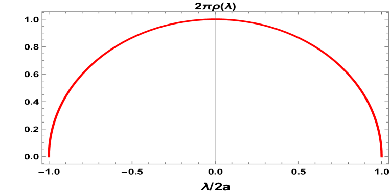
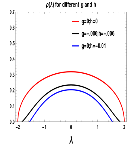
ρ(λ,t)=34λmax32λmax|λ|𝜌𝜆𝑡34superscriptsubscript𝜆𝑚𝑎𝑥32subscript𝜆𝑚𝑎𝑥𝜆\displaystyle\rho(\lambda,t)=\frac{3}{4\lambda_{max}^{\frac{3}{2}}}\sqrt{\lambda_{max}-|\lambda|} (30)

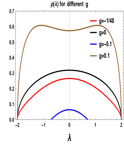
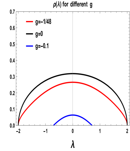
Here λmaxsubscript𝜆𝑚𝑎𝑥\lambda_{max} is the time independent parameter which approximately equals to bound of Lyapunov exponent. This equation shows striking similarity with Wigner law [Eq:-337]. In this approach we can also show the connection between Anderson localization and RMT. But there is a striking difference too. Random matrix theory takes all its entries from Gaussian random variables but for electronic models [Scattering matrix theory] matrix ensemble have short-ranged and sparse random matrix with most of the matrix elements having main diagonal non-zero.

3 Randomness from conduction wire to cosmology: Dynamical study with time dependent protocols

In this section, our objective is to explain the various features from the time dependent effective mass profiles which are related to the quantum mechanical scattering problem in conduction wire as mentioned earlier. These features are appended bellow:

  1. 1.

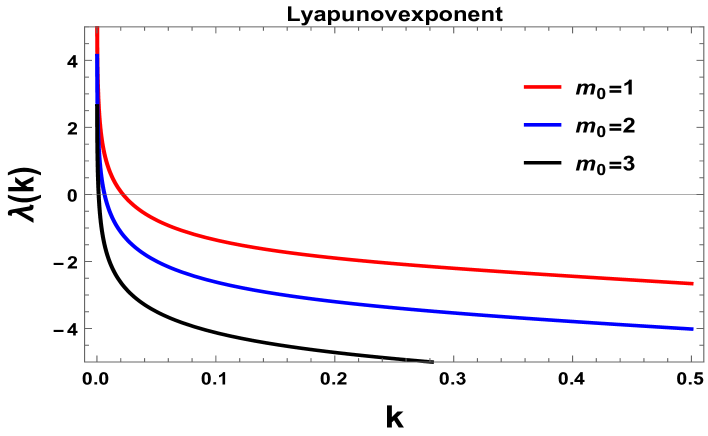
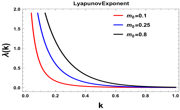
    Lyapunov exponent:  It actually quantify the amount of chaos appearing in the quantum mechanical systems that we are studying in the context of early universe cosmology. In our discussion it tells us the degree of randomness in the stochastic particle production. In our case, the chaos emerges due to the random scattering events which are non adiabatic and we call these as cosmological scattering events leading to particle production. In this section, we discuss about Lyapunov exponent and try to discuss their behaviour for the different time dependent mass profiles. In thus context, Lyapunov exponent is defined as Amin:2015ftc ; Localization1 :

    λ=logT,𝜆log𝑇\displaystyle\lambda=-{\rm log}~{}T, (31)

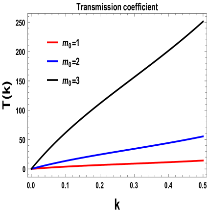
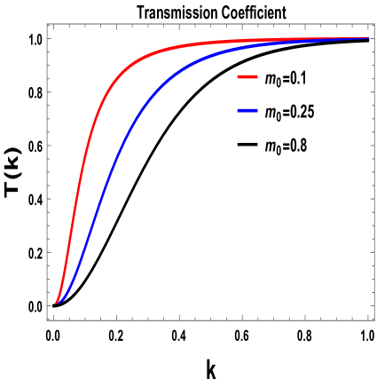
    where, T𝑇T is the transmission coefficient given by the following expression:

    T=tt=|t|2,𝑇superscript𝑡𝑡superscript𝑡2\displaystyle T=t^{*}t=|t|^{2}, (32)

    with t𝑡t and tsuperscript𝑡t^{*} being the transmission amplitude of the incoming and the outgoing wave. In the present discussion, the transmission coefficient can be expressed as:

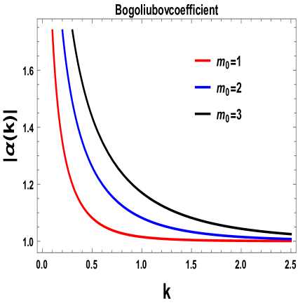
    T=|t|2=1|α|2,𝑇superscript𝑡21superscript𝛼2\displaystyle T=|t|^{2}=\frac{1}{|\alpha|^{2}}, (33)

    where β𝛽\beta and α𝛼\alpha are the Bogoliubov coefficients. Also, it is important to note that, in the present context one can define the reflection coefficient as:

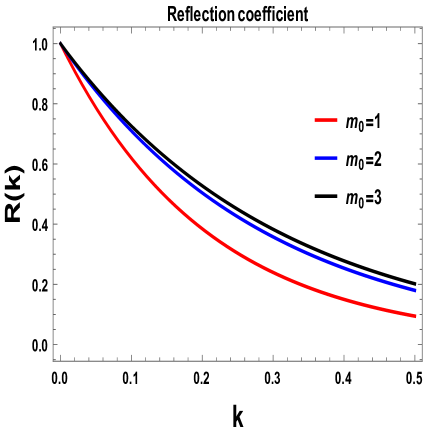
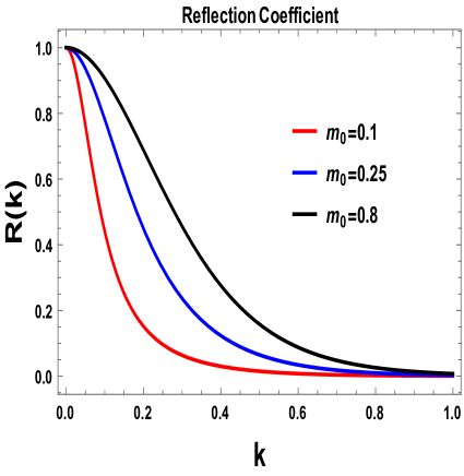
    R=r~r~=|r~|2=|β|2|α|2,𝑅superscript~𝑟~𝑟superscript~𝑟2superscript𝛽2superscript𝛼2\displaystyle R=\tilde{r}^{*}\tilde{r}=|\tilde{r}|^{2}=\frac{|\beta|^{2}}{|\alpha|^{2}}, (34)

    where r~~𝑟\tilde{r} and r~superscript~𝑟\tilde{r}^{*} being the reflection amplitude of the incoming and the outgoing wave. Finally from Eq (6.3.2) and Eq (34), we get the following conservation equation:

    R+T=|r~|2+|t|2=1+|β|2|α|2=1,𝑅𝑇superscript~𝑟2superscript𝑡21superscript𝛽2superscript𝛼21\displaystyle R+T=|\tilde{r}|^{2}+|t|^{2}=\frac{1+|\beta|^{2}}{|\alpha|^{2}}=1, (35)

    where we have used the following normalization condition for the Bogoliubov coefficients, as given by:

    |α|2|β|2=1.superscript𝛼2superscript𝛽21\displaystyle|\alpha|^{2}-|\beta|^{2}=1. (36)
  2. 2.

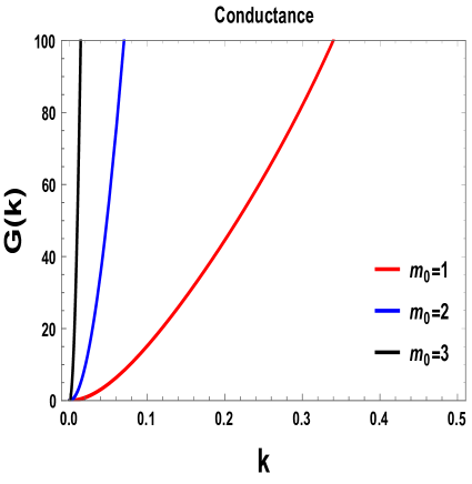
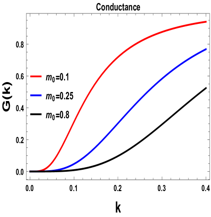
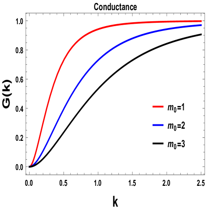
    Conductance:  It quantify the degree of support of the flow of electron inside an electrical conduction wire. this is exactly reciprocal of resistance. In the present context, conductance refers to the ability of the massless scalar fields to transmit through the massive fields which are the specific heavy mass profiles that we have discussed above. This may be more suggestive in telling us about the interaction of the massless scalar field with the massive fields. More value of conductance refers to the larger transmitivity of the background fields through the scatterers and vice-versa. Thus, conductance also carries a valuable information about the transmission coefficient of the scalar field interacting with the scatterer. In this context, the conductance can be expressed as:

    G=exp(2λ)=T2=|t|4=1|α|4,𝐺2𝜆superscript𝑇2superscript𝑡41superscript𝛼4\displaystyle G=\exp\left(-2\lambda\right)=T^{2}=|t|^{4}=\frac{1}{|\alpha|^{4}}~{}~{}, (37)

    where λ𝜆\lambda is the Lyapunov exponent, T𝑇T is the transmission coefficient, |t|𝑡|t| is the transmission amplitude of the incoming/outgoing wave and β,α𝛽𝛼\beta,~{}\alpha are the Bogoliubov coefficients as mentioned above.

  3. 3.

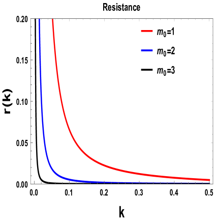
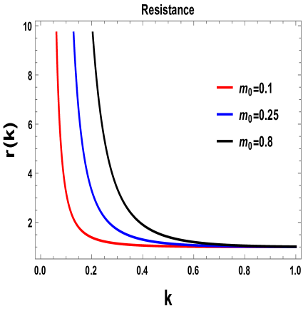
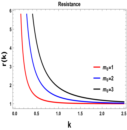
    Resistance:  It quantify the degree of oppose of the flow of electrons inside an electrical conduction wire. It is the property by the virtue of which the scatterers (which are the time dependent mass profiles in our case) resist the massless scalar field to tunnel through them. In other words, it is the same Schrödinger formulation in quantum mechanics where the incoming wave interacts with a potential barrier and the strength of the barrier is the measurement of resistance to the tunneling of the incoming particle through it. This means that more the resistance to the incoming wave, more is the lower is the transmission probability across the barrier. Resistance is defined as the reciprocal of conductance G(k)𝐺𝑘G(k), which gives:

    r(k)=1G(k)=exp(2λ)=1T2=1|t|4=|α|4.𝑟𝑘1𝐺𝑘2𝜆1superscript𝑇21superscript𝑡4superscript𝛼4\displaystyle r(k)=\frac{1}{G(k)}=\exp\left(2\lambda\right)=\frac{1}{T^{2}}=\frac{1}{|t|^{4}}=|\alpha|^{4}~{}~{}. (38)

We will discuss details of these features for three different mass profiles as mentioned in Eq (8). All of these mass profiles that we choose here mimics the role of scatterers inside the conduction wire. Such scatterers provide the way for scattering events to occur resulting in random particle production in cosmological space-time.

To study the cosmological particle creation problem during early epoch of universe (specifically during reheating) we use the analogy with the quantum mechanical scattering problem inside an electrical conduction wire in presence of time dependent effective mass profile we will perform the computation in (quasi) de Sitter space using FLRW spatially flat metric.

Here we consider a massive free scalar field with time-dependent mass  101010Here it is important to note that our approach is similar to that of used in refs. Mandal:2015kxi ; Das:2014hqa to explain the time dynamics of quantum quench. :

S𝑆\displaystyle S =\displaystyle= 12d4xg(gμνμχνχm2(τ)χ2)12superscript𝑑4𝑥𝑔superscript𝑔𝜇𝜈subscript𝜇𝜒subscript𝜈𝜒superscript𝑚2𝜏superscript𝜒2\displaystyle-\frac{1}{2}\int d^{4}x\sqrt{-g}(g^{\mu\nu}\partial_{\mu}\chi~{}\partial_{\nu}\chi-m^{2}(\tau)\chi^{2}) (39)
=\displaystyle= 12d3x𝑑τa2(τ)[(χ(𝐱,τ)τ)2a2(τ){(χ(𝐱,τ))2+m2(τ)(χ(𝐱,τ))2}]12superscript𝑑3𝑥differential-d𝜏superscript𝑎2𝜏delimited-[]superscript𝜒𝐱𝜏𝜏2superscript𝑎2𝜏superscript𝜒𝐱𝜏2superscript𝑚2𝜏superscript𝜒𝐱𝜏2\displaystyle\frac{1}{2}\int d^{3}x~{}d\tau~{}a^{2}(\tau)\left[\left(\frac{\partial\chi({\bf x},\tau)}{\partial\tau}\right)^{2}-a^{2}(\tau)\left\{({\bf\nabla}\chi({\bf x},\tau))^{2}+m^{2}(\tau)(\chi({\bf x},\tau))^{2}\right\}\right]
=\displaystyle= 12d3k(2π)3𝑑τa2(τ)[|dχk(τ)dτ|2a2(τ)(k2+m2(τ))|χk(τ)|2],12superscript𝑑3𝑘superscript2𝜋3differential-d𝜏superscript𝑎2𝜏delimited-[]superscript𝑑subscript𝜒𝑘𝜏𝑑𝜏2superscript𝑎2𝜏superscript𝑘2superscript𝑚2𝜏superscriptsubscript𝜒𝑘𝜏2\displaystyle\frac{1}{2}\int\frac{d^{3}k}{(2\pi)^{3}}d\tau~{}a^{2}(\tau)\left[\left|\frac{d\chi_{k}(\tau)}{d\tau}\right|^{2}-a^{2}(\tau)(k^{2}+m^{2}(\tau))|\chi_{k}(\tau)|^{2}\right],

where the scalar field satisfies the following constraint:

χ(k,τ)=χ(k,τ),𝜒𝑘𝜏superscript𝜒𝑘𝜏\displaystyle\chi(-k,\tau)=\chi^{*}(k,\tau), (40)

and the Fourier transform of the field is defined as:

χ(𝐱,τ)=d3k(2π)3χk(τ)ei𝐤.𝐱.𝜒𝐱𝜏superscript𝑑3𝑘superscript2𝜋3subscript𝜒𝑘𝜏superscript𝑒formulae-sequence𝑖𝐤𝐱\displaystyle\chi({\bf x},\tau)=\int\frac{d^{3}k}{(2\pi)^{3}}\ \chi_{k}(\tau)\ e^{i{\bf k}.{\bf x}}. (41)

Also in the (quasi) de Sitter background the scale factor a(τ)𝑎𝜏a(\tau) can be expressed in terms of conformal time as 111111In de Sitter and quasi de Sitter space one can compute the relation between the conformal time (τ𝜏\tau) and the physical time (t𝑡t) as given by the following expressions: τ=dta={1Ha=1Hexp(Ht),De Sitter1Ha(1+ϵ)=1H(1+ϵ)exp(Ht),Quasi De Sitter ,𝜏𝑑𝑡𝑎cases1𝐻𝑎1𝐻𝐻𝑡De Sittermissing-subexpression1𝐻𝑎1italic-ϵ1𝐻1italic-ϵ𝐻𝑡Quasi De Sitter missing-subexpressionmissing-subexpressionmissing-subexpression\displaystyle\begin{array}[]{lll}\displaystyle\tau=\int\frac{dt}{a}=\left\{\begin{array}[]{lll}\displaystyle-\frac{1}{Ha}=-\frac{1}{H}\exp(-Ht)\,,{}{}{}{}{}{}{}{}{}{}{}{}&\mbox{\small{\color[rgb]{1,0,0}\bf{De Sitter}}}\\ \displaystyle-\frac{1}{Ha}(1+\epsilon)=-\frac{1}{H}(1+\epsilon)\exp(-Ht)\,,{}{}{}{}{}{}{}{}{}{}{}{}&\mbox{\small{\color[rgb]{1,0,0}\bf{Quasi De Sitter }}}\end{array}\right.\end{array}~{}~{}, (45) :

a(τ)={1Hτ,De Sitter1Hτ(1+ϵ),Quasi De Sitter ,𝑎𝜏cases1𝐻𝜏De Sittermissing-subexpression1𝐻𝜏1italic-ϵQuasi De Sitter missing-subexpressionmissing-subexpressionmissing-subexpression\displaystyle\begin{array}[]{lll}\displaystyle a(\tau)=\left\{\begin{array}[]{lll}\displaystyle-\frac{1}{H\tau}\,,{}{}{}{}{}{}{}{}{}{}{}{}&\mbox{\small{\color[rgb]{1,0,0}\bf{De Sitter}}}\\ \displaystyle-\frac{1}{H\tau}(1+\epsilon)\,,{}{}{}{}{}{}{}{}{}{}{}{}&\mbox{\small{\color[rgb]{1,0,0}\bf{Quasi De Sitter }}}\end{array}\right.\end{array}, (49)

where ϵitalic-ϵ\epsilon is the slow-roll parameter in quasi de Sitter space, which is defined as:

ϵ=1H2dHdt=1a(τ)H2dHdτϵ¯a(τ)=Hϵ¯τ.italic-ϵ1superscript𝐻2𝑑𝐻𝑑𝑡1𝑎𝜏superscript𝐻2𝑑𝐻𝑑𝜏¯italic-ϵ𝑎𝜏𝐻¯italic-ϵ𝜏\displaystyle\epsilon=-\frac{1}{H^{2}}\frac{dH}{dt}=-\frac{1}{a(\tau)H^{2}}\frac{dH}{d\tau}\approx\frac{\bar{\epsilon}}{a(\tau)}=-H\bar{\epsilon}\tau. (50)

Here, we define a new slow-roll parameter with respect to the conformal time:

ϵ¯=1H2dHdτ.¯italic-ϵ1superscript𝐻2𝑑𝐻𝑑𝜏\displaystyle\bar{\epsilon}=-\frac{1}{H^{2}}\frac{dH}{d\tau}. (51)

Now we use the following field redefinition in Fourier space:

ϕk(τ)a(τ)χk(τ).subscriptitalic-ϕ𝑘𝜏𝑎𝜏subscript𝜒𝑘𝜏\displaystyle\phi_{k}(\tau)\equiv a(\tau)~{}\chi_{k}(\tau). (52)

Consequently, the scalar field action as stated in Eq (53) can be recast in terms of the newly defined field ϕk(τ)subscriptitalic-ϕ𝑘𝜏\phi_{k}(\tau) as:

S=12d3k(2π)3𝑑τ(|dϕk(τ)dτ1a(τ)da(τ)dτϕk(τ)|2(k2+m2(τ))|ϕk(τ)|2),𝑆12superscript𝑑3𝑘superscript2𝜋3differential-d𝜏superscript𝑑subscriptitalic-ϕ𝑘𝜏𝑑𝜏1𝑎𝜏𝑑𝑎𝜏𝑑𝜏subscriptitalic-ϕ𝑘𝜏2superscript𝑘2superscript𝑚2𝜏superscriptsubscriptitalic-ϕ𝑘𝜏2\displaystyle S=\frac{1}{2}\int\frac{d^{3}k}{(2\pi)^{3}}d\tau~{}\left(\left|\frac{d\phi_{k}(\tau)}{d\tau}-\frac{1}{a(\tau)}\frac{da(\tau)}{d\tau}\phi_{k}(\tau)\right|^{2}-(k^{2}+m^{2}(\tau))|\phi_{k}(\tau)|^{2}\right), (53)

Further, varying the above action with respect to the redefined field ϕk(τ)subscriptsuperscriptitalic-ϕ𝑘𝜏\phi^{*}_{k}(\tau) we get the following equation of motion:

[d2dτ2+1a(τ)da(τ)dτddτ+(k2+m2(τ)(1a(τ)da(τ)dτ)2)]ϕk(τ)=0.delimited-[]superscript𝑑2𝑑superscript𝜏21𝑎𝜏𝑑𝑎𝜏𝑑𝜏𝑑𝑑𝜏superscript𝑘2superscript𝑚2𝜏superscript1𝑎𝜏𝑑𝑎𝜏𝑑𝜏2subscriptitalic-ϕ𝑘𝜏0\displaystyle\left[\frac{d^{2}}{d\tau^{2}}+\frac{1}{a(\tau)}\frac{da(\tau)}{d\tau}\frac{d}{d\tau}+\left(k^{2}+m^{2}(\tau)-\left(\frac{1}{a(\tau)}\frac{da(\tau)}{d\tau}\right)^{2}\right)\right]\phi_{k}(\tau)=0. (54)

Further, Eq (54) can be simplified for de Sitter and quasi de Sitter space as:

𝐃𝐞𝐒𝐢𝐭𝐭𝐞𝐫:¯¯:𝐃𝐞𝐒𝐢𝐭𝐭𝐞𝐫absent\displaystyle\underline{{\color[rgb]{1,0,0}\bf De~{}Sitter:}}~{}~{}~{}~{}~{}~{}~{}~{}~{}~{}~{}~{}~{}~{}~{}~{}~{}~{}~{}~{}~{}~{}~{}~{}~{}~{}~{}~{}~{}~{}~{}~{}~{}~{}~{}~{}~{}~{}~{}~{}~{}\quad\quad\quad~{}~{}~{}~{}~{}~{}~{}~{}~{}~{}~{}~{}~{}~{}~{}~{}~{}~{}~{}~{}~{}~{}~{}~{}~{}~{}~{}~{}~{}~{}~{}~{}~{}~{}~{}~{}~{}~{}
[d2dτ21τddτ+(k2+m2(τ)1τ2)]ϕk(τ)=0.delimited-[]superscript𝑑2𝑑superscript𝜏21𝜏𝑑𝑑𝜏superscript𝑘2superscript𝑚2𝜏1superscript𝜏2subscriptitalic-ϕ𝑘𝜏0\displaystyle\left[\frac{d^{2}}{d\tau^{2}}-\frac{1}{\tau}\frac{d}{d\tau}+\left(k^{2}+m^{2}(\tau)-\frac{1}{\tau^{2}}\right)\right]\phi_{k}(\tau)=0.~{}~{}~{}~{}~{}~{}~{}~{}~{}~{} (55)
𝐐𝐮𝐚𝐬𝐢𝐃𝐞𝐒𝐢𝐭𝐭𝐞𝐫:¯¯:𝐐𝐮𝐚𝐬𝐢𝐃𝐞𝐒𝐢𝐭𝐭𝐞𝐫absent\displaystyle\underline{{\color[rgb]{1,0,0}\bf Quasi~{}De~{}Sitter:}}~{}~{}~{}~{}~{}~{}~{}~{}~{}~{}~{}~{}~{}~{}~{}~{}~{}~{}~{}~{}~{}~{}~{}~{}~{}~{}~{}~{}~{}~{}~{}~{}~{}~{}~{}~{}~{}~{}~{}~{}~{}\quad\quad\quad~{}~{}~{}~{}~{}~{}~{}~{}~{}~{}~{}~{}~{}~{}~{}~{}~{}~{}~{}~{}~{}~{}~{}~{}~{}~{}~{}~{}~{}~{}~{}~{}~{}~{}~{}~{}~{}~{}
[d2dτ21τ(12ϵ21+ϵ)ddτ+(k2+m2(τ)1τ2(12ϵ21+ϵ)2)]ϕk(τ)=0.delimited-[]superscript𝑑2𝑑superscript𝜏21𝜏12superscriptitalic-ϵ21italic-ϵ𝑑𝑑𝜏superscript𝑘2superscript𝑚2𝜏1superscript𝜏2superscript12superscriptitalic-ϵ21italic-ϵ2subscriptitalic-ϕ𝑘𝜏0\displaystyle\left[\frac{d^{2}}{d\tau^{2}}-\frac{1}{\tau}\left(1-\frac{2\epsilon^{2}}{1+\epsilon}\right)\frac{d}{d\tau}+\left(k^{2}+m^{2}(\tau)-\frac{1}{\tau^{2}}\left(1-\frac{2\epsilon^{2}}{1+\epsilon}\right)^{2}\right)\right]\phi_{k}(\tau)=0.~{}~{}~{}~{}~{}~{}~{}~{}~{}~{} (56)

It is important to note that, the main contribution to particle production is originating from the excitations of the field with k/a>>m>>Hmuch-greater-than𝑘𝑎𝑚much-greater-than𝐻k/a>>m>>H, at the stage of oscillations. Therefore, in the first approximation we can neglect the expansion of the Universe, taking the scale factor a(τ)𝑎𝜏a(\tau) as a constant during reheating. We call it reheating approximation 121212Important note: In the present context, the analysis is perfectly valid for the highly localized particle production events after neglecting the cosmological expansion during reheating approximation. But this approximation fail for the events that are sufficiently spaced out. If we don’t neglect the cosmological expansion in this computation then the conformal time dependent mass term of the form 2τ22superscript𝜏22\tau^{2} is restored from the background cosmological background. This actually implies that the scattering problem is being performed on a conformal time dependent potential of the form 1/r21superscript𝑟21/r^{2} (inverse square), which makes the analytic computations of the Bogoliubov coefficients and all the other derived physical quantities to quantify quantum randomness from the present set up extremely difficult. Here it is important to note that, for long wavelength cosmological observables particle production appears more than an e-fold apart and consequently the corrections appearing due to the cosmological expansion seem certainly relevant in the computation as the incoming and outgoing wave functions depart from plane waves. Although for localized particle production events, the reheating approximation considered in this paper perfectly holds good. In the present context this approximation breaks when we consider the particle production events for a sustained period of time or may be separated by times approaching an e-fold expansion. Consequently, one can approximately write Eq (54) in the following simplified form 131313Here it is important to note that, since the scale factor a(τ)𝑎𝜏a(\tau) is approximately a constant during reheating (reheating approximation), then conformal time (τ𝜏\tau) and the physical time (t𝑡t) is related through the following coordinate rescaling transformation: τ=dta=ta.𝜏𝑑𝑡𝑎𝑡𝑎\displaystyle\tau=\int\frac{dt}{a}=\frac{t}{a}. (57) :

[d2dτ2+(k2+m2(τ))]ϕk(τ)=0.delimited-[]superscript𝑑2𝑑superscript𝜏2superscript𝑘2superscript𝑚2𝜏subscriptitalic-ϕ𝑘𝜏0\displaystyle\left[\frac{d^{2}}{d\tau^{2}}+\left(k^{2}+m^{2}(\tau)\right)\right]\phi_{k}(\tau)=0. (58)

The Fourier modes of the scalar field follow the equation of motion in as stated in Eq 58, with every Fourier mode satisfying the Schrödinger equation where m2(τ)superscript𝑚2𝜏-m^{2}(\tau) playing the role of a potential.

Refer to caption
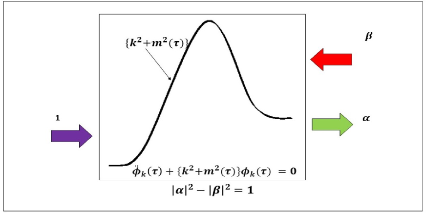
Figure 4: This diagram shows that ground state fluctuations from the past can in future be amplified which can be measured by the coefficient α𝛼\alpha whereas particle excitation from ground state can be measured by β𝛽\beta.

In Fig:4 the particle produced show fluctuation from ground state and from calculating the Bogoliubov coefficients we predicted all its properties. For the solution we refer to ref. Birrell:1982ix , for the field ϕk(τ)subscriptitalic-ϕ𝑘𝜏\phi_{k}(\tau) can be expressed in two distinctive ways, as given by:

ϕk(τ)subscriptitalic-ϕ𝑘𝜏\displaystyle\phi_{k}(\tau) =ain(k)uin(k,τ)+ain(k)uin(k,τ)absentsubscript𝑎𝑖𝑛𝑘subscript𝑢𝑖𝑛𝑘𝜏subscriptsuperscript𝑎𝑖𝑛𝑘subscriptsuperscript𝑢𝑖𝑛𝑘𝜏\displaystyle=a_{in}(k)u_{in}(k,\tau)+a^{\dagger}_{in}(-k)u^{*}_{in}(-k,\tau) (59)
=aout(k)uout(k,τ)+aout(k)uout(k,τ),absentsubscript𝑎𝑜𝑢𝑡𝑘subscript𝑢𝑜𝑢𝑡𝑘𝜏subscriptsuperscript𝑎𝑜𝑢𝑡𝑘subscriptsuperscript𝑢𝑜𝑢𝑡𝑘𝜏\displaystyle=a_{out}(k)u_{out}(k,\tau)+a^{\dagger}_{out}(-k)u^{*}_{out}(-k,\tau),

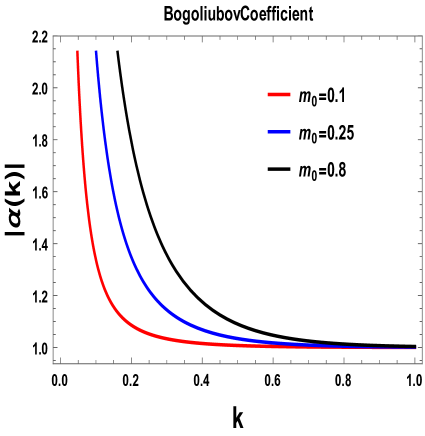
where uin,in(k,τ)subscript𝑢𝑖𝑛𝑖𝑛𝑘𝜏u_{in,in}(k,\tau) and uin,out(k,τ)subscript𝑢𝑖𝑛𝑜𝑢𝑡𝑘𝜏u_{in,out}(k,\tau) are the ‘ingoing’ and ‘outgoing’ wave-functions. Also, the in- and out- oscillators are related to each other through the Bogoliubov coefficients α(k)𝛼𝑘\alpha(k) and β(k)𝛽𝑘\beta(k)

ain(k)subscript𝑎𝑖𝑛𝑘\displaystyle a_{in}(k) =α(k)aout(k)β(k)aout(k),absentsuperscript𝛼𝑘subscript𝑎𝑜𝑢𝑡𝑘superscript𝛽𝑘subscriptsuperscript𝑎𝑜𝑢𝑡𝑘\displaystyle=\alpha^{*}(k)a_{out}(k)-\beta^{*}(k)a^{\dagger}_{out}(-k),
aout(k)subscript𝑎𝑜𝑢𝑡𝑘\displaystyle a_{out}(k) =α(k)ain(k)+β(k)ain(k),absent𝛼𝑘subscript𝑎𝑖𝑛𝑘superscript𝛽𝑘subscriptsuperscript𝑎𝑖𝑛𝑘\displaystyle=\alpha(k)a_{in}(k)+\beta^{*}(k)a^{\dagger}_{in}(-k), (60)

Now, we calculate the various electrical properties and also the expression for the Lyapunov exponent to quantify quantum chaos for the various time dependent effective mass profiles which are equivalent to the impurity potential term in the time Independent Schrödinger Equation describing a scattering problem inside a conduction wire.

3.1 Protocol I: m2(τ)=m02(1tanh(ρτ))/2superscript𝑚2𝜏subscriptsuperscript𝑚201𝜌𝜏2m^{2}(\tau)=m^{2}_{0}(1-\tanh(\rho\tau))/2
Refer to caption
(a) m2(τ)superscript𝑚2𝜏m^{2}(\tau) vs τ𝜏\tau profile.
Refer to caption
(b) V(τ)𝑉𝜏V(\tau) vs τ𝜏\tau profile.
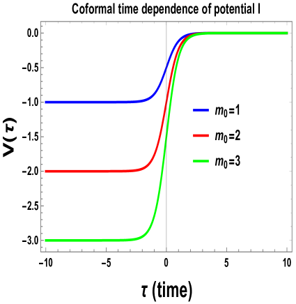
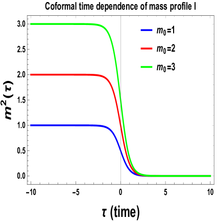
Figure 5: Conformal time dependent behaviour of the mass profile I and its corresponding potential used in Schrödinger scattering problem is explicitly shown here. Here we fix ρ=1𝜌1\rho=1.

Here we start with the following mass profile:

m2(τ)=m02(1tanh(ρτ))/2.superscript𝑚2𝜏subscriptsuperscript𝑚201𝜌𝜏2\displaystyle m^{2}(\tau)=m^{2}_{0}(1-\tanh(\rho\tau))/2. (61)

The corresponding Schrödinger problem for this potential function can be solved by using the potential function as given bellow:

V(τ)=m2(τ)=m02(1tanh(ρτ))/2.𝑉𝜏superscript𝑚2𝜏subscriptsuperscript𝑚201𝜌𝜏2\displaystyle V(\tau)=-m^{2}(\tau)=-m^{2}_{0}(1-\tanh(\rho\tau))/2. (62)

In fig. (5(a)) and fig. (5(b)), we have explicitly shown the conformal time dependent behaviour of the mass profile under consideration and also the corresponding potential used in Schrödinger scattering problem.

We can find the following explicit solutions for uin(k,t)subscript𝑢𝑖𝑛𝑘𝑡u_{in}(k,t) and uout(k,t)subscript𝑢𝑜𝑢𝑡𝑘𝑡u_{out}(k,t), as given by:

uin(k,τ)=eiωinτ2ωin2F1(iωρ,iω+ρ;1iωinρ;e2ρτ),subscript𝑢𝑖𝑛𝑘𝜏subscriptsuperscript𝑒𝑖subscript𝜔𝑖𝑛𝜏2subscript𝜔𝑖𝑛2subscript𝐹1𝑖subscript𝜔𝜌𝑖subscript𝜔𝜌1𝑖subscript𝜔𝑖𝑛𝜌superscript𝑒2𝜌𝜏\displaystyle u_{in}(k,\tau)=\frac{e^{-i\omega_{in}\tau}}{\sqrt{2\omega_{in}}}\;_{2}F_{1}\left(\frac{i\omega_{-}}{\rho},-\frac{i\omega_{+}}{\rho};1-\frac{i\omega_{in}}{\rho};-e^{2\rho\tau}\right), (63)
uout(k,τ)=eiωoutτ2ωout2F1(iωρ,iω+ρ;iωoutρ+1;e2ρτ),subscript𝑢𝑜𝑢𝑡𝑘𝜏subscriptsuperscript𝑒𝑖subscript𝜔𝑜𝑢𝑡𝜏2subscript𝜔𝑜𝑢𝑡2subscript𝐹1𝑖subscript𝜔𝜌𝑖subscript𝜔𝜌𝑖subscript𝜔𝑜𝑢𝑡𝜌1superscript𝑒2𝜌𝜏\displaystyle u_{out}(k,\tau)=\frac{e^{-i\omega_{out}\tau}}{\sqrt{2\omega_{out}}}\;_{2}F_{1}\left(\frac{i\omega_{-}}{\rho},\frac{i\omega_{+}}{\rho};\frac{i\omega_{out}}{\rho}+1;-e^{-2\rho\tau}\right), (64)

where we define ω±subscript𝜔plus-or-minus\omega_{\pm}, ωinsubscript𝜔𝑖𝑛\omega_{in} and ωoutsubscript𝜔𝑜𝑢𝑡\omega_{out} in the following:

ωin=k2+m02,ωout=|k|,ω±=12(ωout±ωin).formulae-sequencesubscript𝜔𝑖𝑛superscript𝑘2superscriptsubscript𝑚02formulae-sequencesubscript𝜔𝑜𝑢𝑡𝑘subscript𝜔plus-or-minus12plus-or-minussubscript𝜔𝑜𝑢𝑡subscript𝜔𝑖𝑛\displaystyle\omega_{in}=\sqrt{k^{2}+m_{0}^{2}},\quad\omega_{out}=|k|,\quad\omega_{\pm}=\frac{1}{2}(\omega_{out}\pm\omega_{in}). (65)

3.1.1 Bogoliubov coefficients

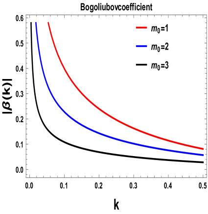
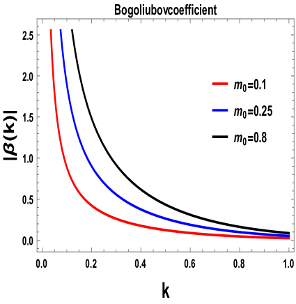
For this specific mass profile the Bogoliubov coefficients can be expressed as:

α(k)=ωoutωinΓ(iωoutρ)Γ(1iωinρ)Γ(iω+2ρ)Γ(1iω+2ρ),β(k)=ωoutωinΓ(iωoutρ)Γ(1iωinρ)Γ(iω2ρ)Γ(1+iω2ρ).formulae-sequence𝛼𝑘subscript𝜔𝑜𝑢𝑡subscript𝜔𝑖𝑛Γ𝑖subscript𝜔𝑜𝑢𝑡𝜌Γ1𝑖subscript𝜔𝑖𝑛𝜌Γ𝑖subscript𝜔2𝜌Γ1𝑖subscript𝜔2𝜌𝛽𝑘subscript𝜔𝑜𝑢𝑡subscript𝜔𝑖𝑛Γ𝑖subscript𝜔𝑜𝑢𝑡𝜌Γ1𝑖subscript𝜔𝑖𝑛𝜌Γ𝑖subscript𝜔2𝜌Γ1𝑖subscript𝜔2𝜌\displaystyle\alpha(k)=\sqrt{\frac{\omega_{out}}{\omega_{in}}}\;\frac{\Gamma\left(-\frac{i\omega_{out}}{\rho}\right)\Gamma\left(1-\frac{i\omega_{in}}{\rho}\right)}{\Gamma\left(-\frac{i\omega_{+}}{2\rho}\right)\Gamma\left(1-\frac{i\omega_{+}}{2\rho}\right)},~{}~{}~{}\beta(k)=\sqrt{\frac{\omega_{out}}{\omega_{in}}}\;\frac{\Gamma\left(\frac{i\omega_{out}}{\rho}\right)\Gamma\left(1-\frac{i\omega_{in}}{\rho}\right)}{\Gamma\left(\frac{i\omega_{-}}{2\rho}\right)\Gamma\left(1+\frac{i\omega_{-}}{2\rho}\right)}.~{}~{}~{}~{} (66)
Refer to caption
(a) α𝛼\alpha vs k𝑘k profile.
Refer to caption
(b) β𝛽\beta vs k𝑘k profile.
Figure 6: Wave number dependence of the Bogoliubov coefficients from the mass profile I is shown here. Here we fix ρ=1𝜌1\rho=1.

In fig. (6(a)) and fig. (6(b)), we have shown the variation of the Bogoliubov Coefficients with wave number k𝑘k.

3.1.2 Optical properties: Reflection and transmission coefficients

For this specific mass profile the transmission and reflection coefficients can be expressed as:

T=1|α(k)|2=ωinωout|Γ(iω+2ρ)Γ(1iω+2ρ)|2|Γ(iωoutρ)Γ(1iωinρ)|2,𝑇1superscript𝛼𝑘2subscript𝜔𝑖𝑛subscript𝜔𝑜𝑢𝑡superscriptΓ𝑖subscript𝜔2𝜌Γ1𝑖subscript𝜔2𝜌2superscriptΓ𝑖subscript𝜔𝑜𝑢𝑡𝜌Γ1𝑖subscript𝜔𝑖𝑛𝜌2\displaystyle T=\frac{1}{|\alpha(k)|^{2}}=\frac{\omega_{in}}{\omega_{out}}\frac{|\Gamma\left(-\frac{i\omega_{+}}{2\rho}\right)\Gamma\left(1-\frac{i\omega_{+}}{2\rho}\right)|^{2}}{|\Gamma\left(-\frac{i\omega_{out}}{\rho}\right)\Gamma\left(1-\frac{i\omega_{in}}{\rho}\right)|^{2}}, (67)
R=|β(k)|2|α(k)|2=|Γ(iωoutρ)|2|Γ(iωoutρ)|2|Γ(iω+2ρ)Γ(1iω+2ρ)|2|Γ(iω2ρ)Γ(1+iω2ρ)|2.𝑅superscript𝛽𝑘2superscript𝛼𝑘2superscriptΓ𝑖subscript𝜔𝑜𝑢𝑡𝜌2superscriptΓ𝑖subscript𝜔𝑜𝑢𝑡𝜌2superscriptΓ𝑖subscript𝜔2𝜌Γ1𝑖subscript𝜔2𝜌2superscriptΓ𝑖subscript𝜔2𝜌Γ1𝑖subscript𝜔2𝜌2\displaystyle R=\frac{|\beta(k)|^{2}}{|\alpha(k)|^{2}}=\frac{|\Gamma\left(\frac{i\omega_{out}}{\rho}\right)|^{2}}{|\Gamma\left(-\frac{i\omega_{out}}{\rho}\right)|^{2}}\frac{|\Gamma\left(-\frac{i\omega_{+}}{2\rho}\right)\Gamma\left(1-\frac{i\omega_{+}}{2\rho}\right)|^{2}}{|\Gamma\left(\frac{i\omega_{-}}{2\rho}\right)\Gamma\left(1+\frac{i\omega_{-}}{2\rho}\right)|^{2}}. (68)
Refer to caption
(a) T(k)𝑇𝑘T(k) vs k𝑘k plot.
Refer to caption
(b) R(k)𝑅𝑘R(k) vs k𝑘k plot.
Figure 7: Wave number dependence of transmission and reflection coefficients for the mass profile I is shown here. Here we fix ρ=1𝜌1\rho=1.

In fig. (7(a)) and fig. (7(b)), we have shown the variation of the transmission and reflection coefficients with wave number k𝑘k.

3.1.3 Chaotic property: Lyapunov exponent

For this specific mass profile the Lyapunov exponent can be expressed as:

λ(k)=logT=2log|α(k)|=2log|ωoutωinΓ(iωoutρ)Γ(1iωinρ)Γ(iω+2ρ)Γ(1iω+2ρ)|.𝜆𝑘𝑇2𝛼𝑘2subscript𝜔𝑜𝑢𝑡subscript𝜔𝑖𝑛Γ𝑖subscript𝜔𝑜𝑢𝑡𝜌Γ1𝑖subscript𝜔𝑖𝑛𝜌Γ𝑖subscript𝜔2𝜌Γ1𝑖subscript𝜔2𝜌\displaystyle\lambda(k)=-\log~{}T=2\log|\alpha(k)|=2\log\left|\sqrt{\frac{\omega_{out}}{\omega_{in}}}\;\frac{\Gamma\left(-\frac{i\omega_{out}}{\rho}\right)\Gamma\left(1-\frac{i\omega_{in}}{\rho}\right)}{\Gamma\left(-\frac{i\omega_{+}}{2\rho}\right)\Gamma\left(1-\frac{i\omega_{+}}{2\rho}\right)}\right|. (69)
Refer to caption
Figure 8: Wave number dependence of Lyapunov exponent is shown for mass profile I. Here we fix ρ=1𝜌1\rho=1.

In fig. 8, we observe that with increase in wave number k𝑘k the Lyapunov exponent decreases. This shows that the Lyapunov exponent is dependent on the momenta values of the fields interacting with the massive field acting as a scatterer. Furthermore, we discover that for the mass profile I, the chaos in the event reduces with increase in the wave number. This suggests that lesser the number of fields interacting with the massive field more is the chaos in the quantum system considered in this paper. Since, a negative value of Lyapunov Exponent pulls a system out of chaos, this further tells us that the Lyapunov exponent is inversely related to the number of background fields interacting with the scatterer or the massive field. This may be interpreted in the following way in the context of Schrödinger problem in quantum mechanics that a higher value of wave number k𝑘k of the incoming wave would be able to cross a potential barrier of a given strength and would be able to get transmitted through the barrier and the pulse won’t damp easily than that of a wave with lower k𝑘k value. This means that the scatterer acts as a definitive medium which allows only certain wave numbers to pass through thus reducing the chaos in the system.

3.1.4 Conduction properties: Conductance and Resistance

For the given mass profile the expression for conductance and resistance can be expressed as:

G(k)=exp(2λ(k))=2log|ωinωoutΓ(iω+2ρ)Γ(1iω+2ρ)Γ(iωoutρ)Γ(1iωinρ)|𝐺𝑘2𝜆𝑘2subscript𝜔𝑖𝑛subscript𝜔𝑜𝑢𝑡Γ𝑖subscript𝜔2𝜌Γ1𝑖subscript𝜔2𝜌Γ𝑖subscript𝜔𝑜𝑢𝑡𝜌Γ1𝑖subscript𝜔𝑖𝑛𝜌\displaystyle~{}G(k)=\exp(-2\lambda(k))=2\log\left|\sqrt{\frac{\omega_{in}}{\omega_{out}}}\;\frac{\Gamma\left(-\frac{i\omega_{+}}{2\rho}\right)\Gamma\left(1-\frac{i\omega_{+}}{2\rho}\right)}{\Gamma\left(-\frac{i\omega_{out}}{\rho}\right)\Gamma\left(1-\frac{i\omega_{in}}{\rho}\right)}\right| (70)
r(k)=exp(2λ(k))=2log|ωoutωinΓ(iωoutρ)Γ(1iωinρ)Γ(iω+2ρ)Γ(1iω+2ρ)|𝑟𝑘2𝜆𝑘2subscript𝜔𝑜𝑢𝑡subscript𝜔𝑖𝑛Γ𝑖subscript𝜔𝑜𝑢𝑡𝜌Γ1𝑖subscript𝜔𝑖𝑛𝜌Γ𝑖subscript𝜔2𝜌Γ1𝑖subscript𝜔2𝜌\displaystyle r(k)=\exp(2\lambda(k))=2\log\left|\sqrt{\frac{\omega_{out}}{\omega_{in}}}\;\frac{\Gamma\left(-\frac{i\omega_{out}}{\rho}\right)\Gamma\left(1-\frac{i\omega_{in}}{\rho}\right)}{\Gamma\left(-\frac{i\omega_{+}}{2\rho}\right)\Gamma\left(1-\frac{i\omega_{+}}{2\rho}\right)}\right| (71)
Refer to caption
(a) G(k)𝐺𝑘G(k) vs k𝑘k plot.
Refer to caption
(b) r(k)𝑟𝑘r(k) vs k𝑘k plot.
Figure 9: Wave number dependence of conductance and resistance for the mass profile I is shown here. Here we fix ρ=1𝜌1\rho=1.

In fig. 9(a) we have shown the variation of conductance with wave number k𝑘k. This figure shows that with increase in the momenta value of the massless scalar field, the conductance also increases. Now, accounting for m0subscript𝑚0m_{0} values, we see that for m0=1subscript𝑚01m_{0}=1 the conductance shoots up at a much lower k𝑘k value than that of m0=2subscript𝑚02m_{0}=2 and m0=3subscript𝑚03m_{0}=3. This suggests that for m0=1subscript𝑚01m_{0}=1 the field has a much higher transmission probability than that of m0=2subscript𝑚02m_{0}=2 and m0=3subscript𝑚03m_{0}=3. An increase in transmission probability gives a direct evidence of the conductance value. Therefore, we conclude that for m0=1subscript𝑚01m_{0}=1 the field has more conductance value in comparison to m0=2subscript𝑚02m_{0}=2 and m0=3subscript𝑚03m_{0}=3. We also conclude that larger the momenta value, more is the transmission coefficient and thereby shoots up the conductance of the system. This means that an incoming wave with large momenta value would eventually cross a barrier potential field thereby increasing the conductance of the system as the transmission probability would be much higher than an incoming wave with lower momenta value.

In fig. 9(b) we have shown the variation of resistance with wave number. We observe that with an increase in the value of k𝑘k the resistance starts decreasing which suggests that with an increase in momenta value the transmission probability across the scatterer. This may be viewed in accordance with the potential barrier in the Schrödinger equation in quantum mechanics also starts increasing thereby allowing the incoming wave to tunnel through the barrier thereby increasing the transmission probability and hence,reducing the resistance. We also observe that with an increase in k𝑘k value the resistance reduces less rapidly for m0=1subscript𝑚01m_{0}=1 than that of m0=3subscript𝑚03m_{0}=3 and m0=2subscript𝑚02m_{0}=2. Whereas, it reduces more rapidly for m0=3subscript𝑚03m_{0}=3 suggesting that higher the value of the constant m0subscript𝑚0m_{0} lower is the value of resistance offered.

3.2 Protocol II: m2(τ)=m02sech2(ρτ)superscript𝑚2𝜏superscriptsubscript𝑚02superscriptsech2𝜌𝜏m^{2}(\tau)=m_{0}^{2}~{}{\rm sech}^{2}(\rho\tau)
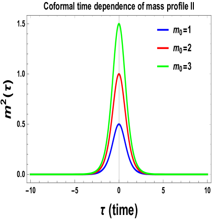
Refer to caption
(a) m2(τ)superscript𝑚2𝜏m^{2}(\tau) vs τ𝜏\tau profile.
Refer to caption
(b) V(τ)𝑉𝜏V(\tau) vs τ𝜏\tau profile.
Figure 10: Conformal time dependent behaviour of the mass profile II and its corresponding potential used in Schrödinger scattering problem is explicitly shown here. Here we fix ρ=1𝜌1\rho=1.

Here we consider the following mass profile:

m2(τ)=m02sech2(ρτ).superscript𝑚2𝜏superscriptsubscript𝑚02superscriptsech2𝜌𝜏\displaystyle~{}m^{2}(\tau)=m_{0}^{2}~{}{\rm sech}^{2}(\rho\tau). (72)

The corresponding Schrödinger problem for this potential function can be solved by using the potential function as given bellow:

V(τ)=m2(τ)=m02sech2(ρτ).𝑉𝜏superscript𝑚2𝜏superscriptsubscript𝑚02superscriptsech2𝜌𝜏\displaystyle V(\tau)=-m^{2}(\tau)=-m_{0}^{2}~{}{\rm sech}^{2}(\rho\tau). (73)

In fig. (10(a)) and fig. (10(b)), we have explicitly shown the conformal time dependent behaviour of the mass profile under consideration and also the corresponding potential used in Schrödinger scattering problem.

Now using the coordinate transformation y=e2ρτ𝑦superscript𝑒2𝜌𝜏y=e^{2\rho\tau} Mandal:2015kxi ; Das:2014hqa one can recast the equation of motion, analogous to the time independent Schrödinger equation takes the following form:

ϕk′′(y)+ϕk(y)y+(k24ρ2y+m02ρ2(1+y)2)ϕk(y)=0.subscriptsuperscriptitalic-ϕ′′𝑘𝑦subscriptsuperscriptitalic-ϕ𝑘𝑦𝑦superscript𝑘24superscript𝜌2𝑦superscriptsubscript𝑚02superscript𝜌2superscript1𝑦2subscriptitalic-ϕ𝑘𝑦0\displaystyle\phi^{\prime\prime}_{k}(y)+\frac{\phi^{\prime}_{k}(y)}{y}+\left(\frac{k^{2}}{4\rho^{2}y}+\frac{m_{0}^{2}}{\rho^{2}(1+y)^{2}}\right)\phi_{k}(y)=0. (74)

The solution of this equation is given by:

u(k,τ)=eikτ(1+e2ρτ)α[C1e2ikτF12(α,ikρ+α,1+ikρ,e2ρτ)+C2F12(α,ikρ+α,1ikρ,e2ρt)],\displaystyle\begin{array}[]{lll}\footnotesize u(k,\tau)=e^{-ik\tau}(1+e^{2\rho\tau})^{\alpha}\left[C_{1}\ e^{2ik\tau}\ {}_{2}F_{1}\left(\alpha,\frac{ik}{\rho}+\alpha,1+\frac{ik}{\rho},-e^{2\rho\tau}\right)\right.\\ \left.~{}~{}~{}~{}~{}+C_{2}\,{}_{2}F_{1}\left(\alpha,-\frac{ik}{\rho}+\alpha,1-\frac{ik}{\rho},-e^{2\rho t}\right)\right],\end{array} (77)

where we define a parameter α𝛼\alpha as:

α=12+1ρ4m02+ρ2𝛼121𝜌4superscriptsubscript𝑚02superscript𝜌2\displaystyle\alpha=\frac{1}{2}+\frac{1}{\rho}\sqrt{4m_{0}^{2}+\rho^{2}} (78)

3.2.1 Bogoliubov coefficients

Now we fix C1=1subscript𝐶11C_{1}=1 and C2=0subscript𝐶20C_{2}=0, which gives the incoming solution uin(k)subscript𝑢𝑖𝑛𝑘u_{in}(k). Further taking the t+𝑡t\to+\infty limit and using Bogoliubov transformation we can express incoming solution in terms of the outgoing solution as given by:

uin(k)=α(k)uout(k)+β(k)uout(k),subscript𝑢𝑖𝑛𝑘𝛼𝑘subscript𝑢𝑜𝑢𝑡𝑘𝛽𝑘subscriptsuperscript𝑢𝑜𝑢𝑡𝑘\displaystyle u_{in}(k)=\alpha(k)u_{out}(k)+\beta(k)u^{*}_{out}(k), (79)

where α(k)𝛼𝑘\alpha(k) and β(k)𝛽𝑘\beta(k) are the Bogoliubov coefficients, which are defined as:

α(k)=Γ(ikρ+1)Γ(ikρ)Γ(ikρα+1)Γ(ikρ+α),β(k)=isin(πα)cosech(πkρ).formulae-sequence𝛼𝑘Γ𝑖𝑘𝜌1Γ𝑖𝑘𝜌Γ𝑖𝑘𝜌𝛼1Γ𝑖𝑘𝜌𝛼𝛽𝑘𝑖𝜋𝛼cosech𝜋𝑘𝜌\displaystyle\alpha(k)=\frac{\Gamma(\frac{ik}{\rho}+1)\Gamma(\frac{ik}{\rho})}{\Gamma(\frac{ik}{\rho}-\alpha+1)\Gamma(\frac{ik}{\rho}+\alpha)},~{}~{}~{}\;\beta(k)=i\sin(\pi\alpha)\text{cosech}\left(\frac{\pi k}{\rho}\right). (80)
Refer to caption
(a) α𝛼\alpha vs k𝑘k profile.
Refer to caption
(b) β𝛽\beta vs k𝑘k profile.
Figure 11: Wave number dependence of the Bogoliubov coefficients are shown here for mass profile II. Here we fix ρ=1𝜌1\rho=1.

In fig. (11(a)) and fig. (11(b)), we have shown the variation of the Bogoliubov coefficients with wave number k𝑘k.

3.2.2 Optical properties: Reflection and transmission coefficients

For this specific mass profile the transmission and the reflection coefficients can be expressed as:

T(K)=1|Γ(ikρ+1)Γ(ikρ)Γ(ikρα+1)Γ(ikρ+α)2|2,R(k)=|isin(πα)cosech(πkρ)|2|Γ(ikρ+1)Γ(ikρ)Γ(ikρα+1)Γ(ikρ+α)|2.formulae-sequence𝑇𝐾1superscriptΓ𝑖𝑘𝜌1Γ𝑖𝑘𝜌Γ𝑖𝑘𝜌𝛼1Γsuperscript𝑖𝑘𝜌𝛼22𝑅𝑘superscript𝑖𝜋𝛼cosech𝜋𝑘𝜌2superscriptΓ𝑖𝑘𝜌1Γ𝑖𝑘𝜌Γ𝑖𝑘𝜌𝛼1Γ𝑖𝑘𝜌𝛼2\displaystyle T(K)=\frac{1}{|\frac{\Gamma(\frac{ik}{\rho}+1)\Gamma(\frac{ik}{\rho})}{\Gamma(\frac{ik}{\rho}-\alpha+1)\Gamma(\frac{ik}{\rho}+\alpha)^{2}}|^{2}},~{}~{}~{}~{}\;R(k)=\frac{|i\sin(\pi\alpha)\text{cosech}\left(\frac{\pi k}{\rho}\right)|^{2}}{|\frac{\Gamma(\frac{ik}{\rho}+1)\Gamma(\frac{ik}{\rho})}{\Gamma(\frac{ik}{\rho}-\alpha+1)\Gamma(\frac{ik}{\rho}+\alpha)}|^{2}}. (81)
Refer to caption
(a) T(k)𝑇𝑘T(k) vs k𝑘k plot.
Refer to caption
(b) R(k)𝑅𝑘R(k) vs k𝑘k plot.
Figure 12: Transmission and Reflection Coefficient for mass profile m2(t)=m02sech2(ρτ)superscript𝑚2𝑡superscriptsubscript𝑚02𝑠𝑒𝑐superscript2𝜌𝜏m^{2}(t)=m_{0}^{2}sech^{2}(\rho\tau)

In fig. (12(a)) and fig. (12(b)), we have shown the variation of the transmission and reflection coefficients with wave number k𝑘k.

3.2.3 Chaotic property: Lyapunov exponent

The Lyapunov exponent for this case may be given as:

λ=logT=2log|α(k)|=2log|Γ(ikρ+1)Γ(ikρ)Γ(ikρα+1)Γ(ikρ+α)2|.𝜆𝑇2𝛼𝑘2Γ𝑖𝑘𝜌1Γ𝑖𝑘𝜌Γ𝑖𝑘𝜌𝛼1Γsuperscript𝑖𝑘𝜌𝛼2\displaystyle\lambda=-\log~{}T=2\log|\alpha(k)|=2\log\left|\frac{\Gamma(\frac{ik}{\rho}+1)\Gamma(\frac{ik}{\rho})}{\Gamma(\frac{ik}{\rho}-\alpha+1)\Gamma(\frac{ik}{\rho}+\alpha)^{2}}\right|. (82)
Refer to caption
Figure 13: This shows the variation of Lyapunov exponent with momenta values for mass profiles with m0=1subscript𝑚01m_{0}=1, m0=2subscript𝑚02m_{0}=2 and m0=3subscript𝑚03m_{0}=3

In fig. 13, we have shown the wave number dependence of Lyapunov exponent. Here we observe that with increase in k𝑘k value the Lyapunov exponent decreases. This implies that the Lyapunov exponent is dependent on the momenta values of the fields interacting with the massive field acting as a scatterer. Furthermore, we also discover that for this mass profile II, the chaos in the event reduces with increase in the k𝑘k value.

3.2.4 Conduction properties: Conductance and Resistance

For this specific mass profile the expression for the conductance and resistance can be computed as:

G(k)=exp(2λ(k))=|Γ(ikρ+1)Γ(ikρ)Γ(ikρα+1)Γ(ikρ+α)2|4,𝐺𝑘2𝜆𝑘superscriptΓ𝑖𝑘𝜌1Γ𝑖𝑘𝜌Γ𝑖𝑘𝜌𝛼1Γsuperscript𝑖𝑘𝜌𝛼24\displaystyle G(k)=\exp(-2\lambda(k))=\left|\frac{\Gamma(\frac{ik}{\rho}+1)\Gamma(\frac{ik}{\rho})}{\Gamma(\frac{ik}{\rho}-\alpha+1)\Gamma(\frac{ik}{\rho}+\alpha)^{2}}\right|^{4}, (83)
r(k)=exp(2λ(k))=|Γ(ikρα+1)Γ(ikρ+α)2Γ(ikρ+1)Γ(ikρ)|4.𝑟𝑘2𝜆𝑘superscriptΓ𝑖𝑘𝜌𝛼1Γsuperscript𝑖𝑘𝜌𝛼2Γ𝑖𝑘𝜌1Γ𝑖𝑘𝜌4\displaystyle r(k)=\exp(2\lambda(k))=\left|\frac{\Gamma(\frac{ik}{\rho}-\alpha+1)\Gamma(\frac{ik}{\rho}+\alpha)^{2}}{\Gamma(\frac{ik}{\rho}+1)\Gamma(\frac{ik}{\rho})}\right|^{4}. (84)
Refer to caption
(a) G(k)𝐺𝑘G(k) vs k𝑘k plot.
Refer to caption
(b) r(k)𝑟𝑘r(k) vs k𝑘k plot.
Figure 14: Wave number dependence of conductance and resistance for the mass profile II is shown here. Here we fix ρ=1𝜌1\rho=1.

In fig. 14(a) we have shown the wave number dependence of conductance. We observe that for m0=1subscript𝑚01m_{0}=1 conductance starts increasing at a larger value of k𝑘k than that of m0=2subscript𝑚02m_{0}=2 and m0=3subscript𝑚03m_{0}=3. But, in contrast to the variation of conductance with momenta k𝑘k in the above figure, here the conductance starts increasing rapidly for m0=3subscript𝑚03m_{0}=3 than that for m0=1subscript𝑚01m_{0}=1 which suggests that the transmission probability for m0=3subscript𝑚03m_{0}=3 is much higher than m0=1subscript𝑚01m_{0}=1 and m0=2subscript𝑚02m_{0}=2, thereby making it more conductive than the other two.

In fig. 14(b), we have shown the wave number dependence of resistance. Here like the first mass profile the resistance for m0=3subscript𝑚03m_{0}=3 falls more rapidly than that of m0=2subscript𝑚02m_{0}=2 and m0=1subscript𝑚01m_{0}=1. This suggests that for the given mass profile II, as the value of m0subscript𝑚0m_{0} increases, the value of resistance also decreases. But unlike the first mass profile, the resistance for m0=3subscript𝑚03m_{0}=3 falls more rapidly suggesting that for m0=3subscript𝑚03m_{0}=3 this specific mass profile offers more resistance than the first one. Therefore, we conclude that for the same values of m0subscript𝑚0m_{0} this mass profile offers less resistance in comparison to the first mass profile.

3.3 Protocol III: m2(τ)=m02Θ(τ)superscript𝑚2𝜏superscriptsubscript𝑚02Θ𝜏m^{2}(\tau)=m_{0}^{2}~{}\Theta(-\tau)
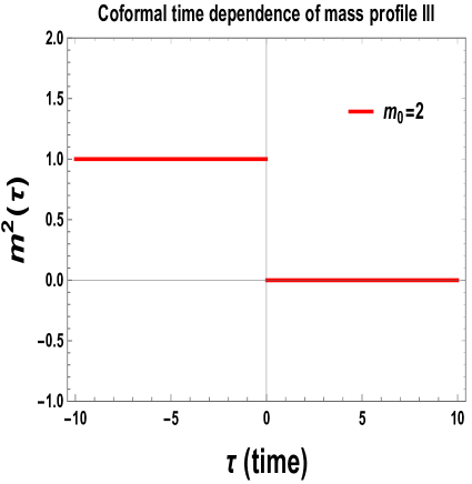
Refer to caption
(a) m2(τ)superscript𝑚2𝜏m^{2}(\tau) vs τ𝜏\tau profile.
Refer to caption
(b) V(τ)𝑉𝜏V(\tau) vs τ𝜏\tau profile.
Figure 15: Conformal time dependent behaviour of the mass profile II and its corresponding potential used in Schrödinger scattering problem is explicitly shown here.

Here we consider the following time dependent mass profile:

m2(τ)=m02Θ(τ).superscript𝑚2𝜏superscriptsubscript𝑚02Θ𝜏\displaystyle m^{2}(\tau)=m_{0}^{2}~{}\Theta(-\tau). (85)

This ΘΘ\Theta function in τ𝜏\tau makes the mass profile a quenched one.

The corresponding Schrödinger problem for this potential function can be solved by using the potential function as given bellow:

V(τ)=m2(τ)=m02Θ(τ).𝑉𝜏superscript𝑚2𝜏superscriptsubscript𝑚02Θ𝜏\displaystyle V(\tau)=-m^{2}(\tau)=-m_{0}^{2}~{}\Theta(-\tau). (86)

In fig. (15(a)) and fig. (15(b)), we have explicitly shown the conformal time dependent behaviour of the mass profile under consideration and also the corresponding potential used in Schrödinger scattering problem.

3.3.1 Bogoliubov coefficients

For this specific mass profile the Bogoliubov coefficients can be expressed as:

α(k)=12|k|+ωin|k|ωin,β(k)=12|k|ωin|k|ωin.formulae-sequence𝛼𝑘12𝑘subscript𝜔𝑖𝑛𝑘subscript𝜔𝑖𝑛𝛽𝑘12𝑘subscript𝜔𝑖𝑛𝑘subscript𝜔𝑖𝑛\displaystyle\alpha(k)=\frac{1}{2}\frac{|k|+\omega_{in}}{\sqrt{|k|\omega_{in}}},~{}~{}~{}~{}\;\beta(k)=\frac{1}{2}\frac{|k|-\omega_{in}}{\sqrt{|k|\omega_{in}}}. (87)

with the solution of the incoming and the outgoing waves are given by the following expressions:

uin(k,t)=eiωint2ωin,uout(k,t)=eiωoutt2ωout.formulae-sequencesubscript𝑢𝑖𝑛𝑘𝑡superscript𝑒𝑖subscript𝜔𝑖𝑛𝑡2subscript𝜔𝑖𝑛subscript𝑢𝑜𝑢𝑡𝑘𝑡superscript𝑒𝑖subscript𝜔𝑜𝑢𝑡𝑡2subscript𝜔𝑜𝑢𝑡\displaystyle u_{in}(k,t)=\frac{e^{-i\omega_{in}t}}{\sqrt{2\omega_{in}}},~{}~{}~{}u_{out}(k,t)=\frac{e^{-i\omega_{out}t}}{\sqrt{2\omega_{out}}}. (88)
Refer to caption
(a) α𝛼\alpha vs k𝑘k profile.
Refer to caption
(b) β𝛽\beta vs k𝑘k profile.
Figure 16: Wave number dependence of Bogoliubov coefficients for mass profile II is shown here.

In fig. (17(a)) and fig. (16(b)), we have shown the variation of the transmission and reflection coefficients with wave number k𝑘k.

3.3.2 Optical properties: Refeclection and transmission coefficients

For this specific mass profile the transmission and the reflection coefficients can be computed as:

T(k)=|2|k|ωin|k|+ωin|2,R(k)=|2|k|ωin|k|ωin|2.formulae-sequence𝑇𝑘superscript2𝑘subscript𝜔𝑖𝑛𝑘subscript𝜔𝑖𝑛2𝑅𝑘superscript2𝑘subscript𝜔𝑖𝑛𝑘subscript𝜔𝑖𝑛2\displaystyle T(k)=\left|\frac{2\sqrt{|k|\omega_{in}}}{|k|+\omega_{in}}\right|^{2},~{}~{}~{}R(k)=\left|\frac{2\sqrt{|k|\omega_{in}}}{|k|-\omega_{in}}\right|^{2}. (89)
Refer to caption
(a) T(k)𝑇𝑘T(k) vs k𝑘k plot.
Refer to caption
(b) R(k)𝑅𝑘R(k) vs k𝑘k plot.
Figure 17: Wave number dependence of the transmission and reflection coefficients for mass profile III is shown here.

In fig. (17(a)) and fig. (17(b)), we have shown the variation of the transmission and reflection coefficients with wave number k𝑘k.

3.3.3 Chaotic property: Lyapunov exponent

The Lyapunov in this case is written as:

λ=2logT=2log|α(k)|=2log|12|k|+ωin|k|ωin|.𝜆2𝑇2𝛼𝑘212𝑘subscript𝜔𝑖𝑛𝑘subscript𝜔𝑖𝑛\displaystyle\lambda=-2\log~{}T=2\log|\alpha(k)|=2\log\left|\frac{1}{2}\frac{|k|+\omega_{in}}{\sqrt{|k|\omega_{in}}}\right|. (90)
Refer to caption
Figure 18: Variation of Lyapunov exponent is shown with respect to the wave number.

From fig. 18 we observe that with increase in wave number the Lyapunov exponent decreases more like a rectangular hyperbolic fashion. In comparison to the other two mass profiles where the reduction in the value of the Lyapunov exponent is much less rapid in comparison to this mass profile discussed here. This suggests that since, the mass profile is a heavy side theta function, which is a quenched mass protocol, the Lyapunov exponent also gives a similar like profile. This shows that the Lyapunov exponent is dependent on the wave number of the fields interacting with the massive field acting as a scatterer. Furthermore, we discover that for this given mass profile, the chaos in the event reduces with increase in the k𝑘k value. So, in this case the Lyapunov exponent decays much rapidly than the first two mass profiles. Next, we will try to find an upper bound of Lyapunov exponent using the definition of RMT

3.3.4 Conduction properties: Conductance and Resistance

For this specific mass profile the expression for the conductance and resistance can be written as:

G(k)=exp(2λ(k))=|2|k|ωin|k|+ωin|4,𝐺𝑘2𝜆𝑘superscript2𝑘subscript𝜔𝑖𝑛𝑘subscript𝜔𝑖𝑛4\displaystyle G(k)=\exp(-2\lambda(k))=\left|\frac{2\sqrt{|k|\omega_{in}}}{|k|+\omega_{in}}\right|^{4}, (91)
r(k)=exp(2λ(k))=|12|k|+ωin|k|ωin|4,𝑟𝑘2𝜆𝑘superscript12𝑘subscript𝜔𝑖𝑛𝑘subscript𝜔𝑖𝑛4\displaystyle r(k)=\exp(2\lambda(k))=\left|\frac{1}{2}\frac{|k|+\omega_{in}}{\sqrt{|k|\omega_{in}}}\right|^{4}, (92)
Refer to caption
(a) G(k)𝐺𝑘G(k) vs k𝑘k plot.
Refer to caption
(b) r(k)𝑟𝑘r(k) vs k𝑘k plot.
Figure 19: Wave number dependence of conductance and resistance for the mass profile III is shown here.

In fig. 19(a), we have shown the wave number dependence of conductance. This figure shows that with increase in the wave number of the massless scalar field, the conductance also increases. Now, accounting for m0subscript𝑚0m_{0} values, we see that for m0=1subscript𝑚01m_{0}=1 the conductance shoots up at a much lower k𝑘k value than that of m0=2subscript𝑚02m_{0}=2 and m0=3subscript𝑚03m_{0}=3. This suggests that for m0=1subscript𝑚01m_{0}=1 the field has a much higher transmission probability than that of m0=2subscript𝑚02m_{0}=2 and m0=3subscript𝑚03m_{0}=3. An increase in transmission probability gives a direct evidence of the conductance value. Therefore, we conclude that for m0=1subscript𝑚01m_{0}=1 the field has more conductance value in comparison to m0=2subscript𝑚02m_{0}=2 and m0=3subscript𝑚03m_{0}=3.

In fig. 19(b), unlike the mass profile I the resistance for m0=1subscript𝑚01m_{0}=1 falls more rapidly than that of m0=2subscript𝑚02m_{0}=2 and m0=3subscript𝑚03m_{0}=3. This suggest that for the given mass profile, as the value of m0subscript𝑚0m_{0} increases, the value of resistance also increases suggesting that heavier the field gets lesser is the transmission probability of the incoming wave to tunnel through it thereby reducing the value of conductance for this specific mass profile.

4 Quantum chaos from out of time ordered correlators (OTOC)

4.1 Chaos bound in out-of-equilibrium quantum field theory (OEQFT) and its application to cosmology

We know that in the context of quantum field theory it is possible to achieve the following universal bound on the Lyapunov exponent Maldacena:2015waa  141414For this specific discussion only we keep the Planck’s constant Planck-constant-over-2-pi\hbar and the Boltzmann constant kBsubscript𝑘𝐵k_{B} in our computation. But for the rest of the paper we fix =1Planck-constant-over-2-pi1\hbar=1 and kB=1subscript𝑘𝐵1k_{B}=1 for which the parameter β𝛽\beta can be written as, β=1/T𝛽1𝑇\beta=1/T. In such a situation chaos bound is given by, λ<2π/β𝜆2𝜋𝛽\lambda<2\pi/\beta. 151515In the context of weakly coupled gauge theory one can introduce ’t Hooft coupling λTsubscript𝜆𝑇\lambda_{T} which is independent of N𝑁N and in such a theory the Lyapunov exponent is given by the following expression: 𝐋𝐲𝐚𝐩𝐮𝐧𝐨𝐯𝐞𝐱𝐩𝐨𝐧𝐞𝐧𝐭𝐢𝐧𝐠𝐚𝐮𝐠𝐞𝐭𝐡𝐞𝐨𝐫𝐲:¯λG=λTβ=λTkBT=λT2π2πkBT<λ¯:𝐋𝐲𝐚𝐩𝐮𝐧𝐨𝐯𝐞𝐱𝐩𝐨𝐧𝐞𝐧𝐭𝐢𝐧𝐠𝐚𝐮𝐠𝐞𝐭𝐡𝐞𝐨𝐫𝐲absentsubscript𝜆𝐺subscript𝜆𝑇𝛽subscript𝜆𝑇subscript𝑘𝐵𝑇Planck-constant-over-2-pisubscript𝜆𝑇2𝜋2𝜋subscript𝑘𝐵𝑇Planck-constant-over-2-pi𝜆\displaystyle{{\color[rgb]{0,0,1}\bf\underline{Lyapunov~{}exponent~{}in~{}gauge~{}theory:}}}~{}~{}~{}~{}~{}~{}~{}~{}\lambda_{G}=\frac{\lambda_{T}}{\beta}=\lambda_{T}k_{B}T=\frac{\hbar\lambda_{T}}{2\pi}\frac{2\pi k_{B}T}{\hbar}<\lambda (93) :

𝐔𝐧𝐢𝐯𝐞𝐫𝐬𝐚𝐥𝐜𝐡𝐚𝐨𝐬𝐛𝐨𝐮𝐧𝐝𝐢𝐧𝐎𝐄𝐐𝐅𝐓:¯λ2πkBT=2πβ,¯:𝐔𝐧𝐢𝐯𝐞𝐫𝐬𝐚𝐥𝐜𝐡𝐚𝐨𝐬𝐛𝐨𝐮𝐧𝐝𝐢𝐧𝐎𝐄𝐐𝐅𝐓absent𝜆2𝜋subscript𝑘𝐵𝑇Planck-constant-over-2-pi2𝜋Planck-constant-over-2-pi𝛽\displaystyle{{\color[rgb]{0,0,1}\bf\underline{Universal~{}chaos~{}bound~{}in~{}OEQFT:}}}~{}~{}~{}~{}~{}~{}~{}~{}\lambda\leq\frac{2\pi k_{B}T}{\hbar}=\frac{2\pi}{\hbar\beta}, (94)

where kBsubscript𝑘𝐵k_{B} is the Boltzmann constant and T𝑇T is the temperature associated with the dynamical system. This upper bound of the Lyapunov exponent is treated as the saturation bound of chaos 161616Considering the bulk contribution weakly coupled with string theory with large radius of curvature one can show that the perturbative stringy correction to the Einstein gravity computation of the scrambling can give rise to the following first order corrected expression for the Lyapunov exponent : 𝐒𝐭𝐫𝐢𝐧𝐠𝐲𝐜𝐨𝐫𝐫𝐞𝐜𝐭𝐢𝐨𝐧:λ=2πβ[1μ22Ls2+𝐒𝐭𝐫𝐢𝐧𝐠𝐲𝐜𝐨𝐫𝐫𝐞𝐜𝐭𝐢𝐨𝐧],\displaystyle{\color[rgb]{0,0,1}\bf Stringy~{}correction:}~{}~{}~{}~{}\lambda=\frac{2\pi}{\beta}\left[1-\underbrace{\frac{\mu^{2}}{2}L_{s}^{2}+\cdots}_{{\color[rgb]{1,0,0}\bf Stringy~{}correction}}\right], (95) where Lssubscript𝐿𝑠L_{s} is the stringy length scale and μ2superscript𝜇2\mu^{2} is a specific constant which is appearing in the shock wave equation propagating along the horizon. . Our aim is to establish this bound in the context of cosmology and study its further consequences. This bound was first proposed in the context of quantum information theory of black hole chaosblackhole ; Lowe:2017ehz ; Polchinski:2016hrw ; Polchinski:2015cea . Additionally it is important that, the bound on the Lyapunov exponent saturates in the context of Sachdev-Ye-Kitaev (SYK) model Maldacena:2016hyu ; Choudhury:2017tax ; Mandal:2017thl ; Gross:2017hcz ; Das:2017pif ; Garcia-Garcia:2016mno ; Garcia-Garcia:2017pzl ; Witten:2016iux ; Nishinaka:2016nxg , which describes the quantum features of Majorana fermions in presence of infinitely long range disorder. Saturation of the Lyapunov exponent implies that SYK model mimics a quantum description of black hole via AdS/CFT correspondence. In the strict classical limit 0Planck-constant-over-2-pi0\hbar\rightarrow 0 the Lyapunov exponent take any values, which is consistent with the requirement.

To give an explicit derivation of the chaos bound on Lyapunov exponent in the context of cosmology let us follow the steps appended below:

  1. 1.

    Let us start with a completely mathematical problem described by a time dependent function g(τ)𝑔𝜏g(\tau), which satisfy the following set of properties:

    1. (a)

      In the complex plane g(τ+iT)𝑔𝜏𝑖𝑇g(\tau+iT) is analytic in the half strip described within τ>0𝜏0\tau>0 and β4Tβ4𝛽4𝑇𝛽4-\frac{\beta}{4}\leq T\leq\frac{\beta}{4}. In this context, τ𝜏\tau and T𝑇T represent the real and imaginary part of the complex number τ+iT𝜏𝑖𝑇\tau+iT after analytical continuation in complex plane.

    2. (b)

      The function g(τ)𝑔𝜏g(\tau) is completely real at T=0𝑇0T=0.

    3. (c)

      After analytical continuation the function in the complex plane satisfy the following constraint:

      |g(τ+iT)|1,𝑔𝜏𝑖𝑇1|g(\tau+iT)|\leq 1, (96)

      which is perfectly valid in the complete half strip.

  2. 2.

    Next, we actually conformally map the entire half strip to a unit thermal circle in the complex plane, which can be done using the following Mo¨¨𝑜\ddot{o}bius transformation:

    𝐌𝐨¨𝐛𝐢𝐮𝐬𝐭𝐫𝐚𝐧𝐬𝐟𝐨𝐫𝐦𝐚𝐭𝐢𝐨𝐧:¯z=1Δβ(τ+iT)1+Δβ(τ+iT),¯:𝐌¨𝐨𝐛𝐢𝐮𝐬𝐭𝐫𝐚𝐧𝐬𝐟𝐨𝐫𝐦𝐚𝐭𝐢𝐨𝐧absent𝑧1subscriptΔ𝛽𝜏𝑖𝑇1subscriptΔ𝛽𝜏𝑖𝑇\displaystyle{\color[rgb]{0,0,1}\bf\underline{M\ddot{o}bius~{}transformation:}}~{}~{}~{}~{}z=\frac{1-\Delta_{\beta}(\tau+iT)}{1+\Delta_{\beta}(\tau+iT)}, (97)

    where Δβ(τ+iT)subscriptΔ𝛽𝜏𝑖𝑇\Delta_{\beta}(\tau+iT) is the temperature dependent function in the complex plane, described by the following expression:

    Δβ(τ+iT):=sinh(2πβ(τ+iT)).assignsubscriptΔ𝛽𝜏𝑖𝑇2𝜋𝛽𝜏𝑖𝑇\displaystyle\Delta_{\beta}(\tau+iT):=\sinh\left(\frac{2\pi}{\beta}(\tau+iT)\right). (98)
    Refer to caption
    (a) |z|𝑧|z| with β=1𝛽1\beta=1.
    Refer to caption
    (b) z with β=1𝛽1\beta=1 and T=0𝑇0T=0.
    Figure 20: Parametric dependence |z|𝑧|z| and z(T=0)𝑧𝑇0z(T=0) at different temperatures.

    In fig. (20(a)), we have shown the behaviour of the amplitude of the complex number z𝑧z with respect to the parameters (τ,T𝜏𝑇\tau,T) in 3D plot. Finally, to check the consistency with Schwarz-Pick inequality we have plotted the complex number z𝑧z at T=0𝑇0T=0 in fig. (20(b)).

  3. 3.

    Further using Eq (96) one can further say that the complex function g(z)𝑔𝑧g(z) is an analytic function from one to one conformal map from unit disk to unit disk.

  4. 4.

    A variant of the Schwarz lemma can be represented as a invariant contribution under analytic automorphisms on the unit disk, which implies the bijective holomorphic mappings of the unit disc to itself. This specific variant is known as the Schwarz–Pick theorem.

  5. 5.

    Now the hyperbolic metric in complex plane is defined as:

    ds2=4dzdz¯(1|z|2)2=(2|dz|(1|z|2))2.𝑑superscript𝑠24𝑑𝑧𝑑¯𝑧superscript1superscript𝑧22superscript2𝑑𝑧1superscript𝑧22\displaystyle ds^{2}=4\frac{dzd\bar{z}}{\left(1-|z|^{2}\right)^{2}}=\left(\frac{2|dz|}{\left(1-|z|^{2}\right)}\right)^{2}. (99)

    Further using this metric and applying Schwarz–Pick theorem one can write:

    𝐒𝐜𝐡𝐰𝐚𝐫𝐳𝐏𝐢𝐜𝐤𝐢𝐧𝐞𝐪𝐮𝐚𝐥𝐢𝐭𝐲:¯|dg|(1|g(z)|2)ds=2|dz|(1|z|2).¯:𝐒𝐜𝐡𝐰𝐚𝐫𝐳𝐏𝐢𝐜𝐤𝐢𝐧𝐞𝐪𝐮𝐚𝐥𝐢𝐭𝐲absent𝑑𝑔1superscript𝑔𝑧2𝑑𝑠2𝑑𝑧1superscript𝑧2\displaystyle{\color[rgb]{0,0,1}\bf\underline{Schwarz–Pick~{}inequality:}}~{}~{}~{}~{}\frac{|dg|}{\left(1-|g(z)|^{2}\right)}\leq ds=\frac{2|dz|}{\left(1-|z|^{2}\right)}. (100)
  6. 6.

    Further applying the fact that the function g(τ)𝑔𝜏g(\tau) is real at T=0𝑇0T=0 and using Eq (100) we get the following simplified result:

    11g2(τ)|dg(τ)dτ|[11|z|2|dzdτ|]T=0=πβcoth(2πτβ).11superscript𝑔2𝜏𝑑𝑔𝜏𝑑𝜏subscriptdelimited-[]11superscript𝑧2𝑑𝑧𝑑𝜏𝑇0𝜋𝛽hyperbolic-cotangent2𝜋𝜏𝛽\displaystyle\frac{1}{1-g^{2}(\tau)}\left|\frac{dg(\tau)}{d\tau}\right|\leq\left[\frac{1}{1-|z|^{2}}\left|\frac{dz}{d\tau}\right|\right]_{T=0}=\frac{\pi}{\beta}\coth\left(\frac{2\pi\tau}{\beta}\right). (101)
  7. 7.

    Further, rearranging Eq (101) we get the following final result:

    1(1g(τ))|dg(τ)dτ|12(1+g(τ))2πβcoth(2πτβ),11𝑔𝜏𝑑𝑔𝜏𝑑𝜏121𝑔𝜏2𝜋𝛽hyperbolic-cotangent2𝜋𝜏𝛽\displaystyle\frac{1}{(1-g(\tau))}\left|\frac{dg(\tau)}{d\tau}\right|\leq\frac{1}{2}(1+g(\tau))\frac{2\pi}{\beta}\coth\left(\frac{2\pi\tau}{\beta}\right), (102)

    which is the outcome of Schwarz-Pick inequality and very very useful to prove the universal chaos bound in OEQFT.

    Now it is important to note that in this context,

    12(1+g(τ))coth(2πτβ)1+β2π𝒪(exp(4πτβ)).121𝑔𝜏hyperbolic-cotangent2𝜋𝜏𝛽1𝛽2𝜋𝒪4𝜋𝜏𝛽\displaystyle\frac{1}{2}(1+g(\tau))\coth\left(\frac{2\pi\tau}{\beta}\right)\leq 1+\frac{\beta}{2\pi}{\cal O}\left(\exp\left(-\frac{4\pi\tau}{\beta}\right)\right).~{} (103)

    This further implies that:

    1(1g(τ))|dg(τ)dτ|2πβ+𝒪(exp(4πτβ)).11𝑔𝜏𝑑𝑔𝜏𝑑𝜏2𝜋𝛽𝒪4𝜋𝜏𝛽\displaystyle\frac{1}{(1-g(\tau))}\left|\frac{dg(\tau)}{d\tau}\right|\leq\frac{2\pi}{\beta}+{\cal O}\left(\exp\left(-\frac{4\pi\tau}{\beta}\right)\right). (104)

    Now at very large time scale (τ𝜏\tau\rightarrow\infty) or at very high temperature (β=1/T0𝛽1𝑇0\beta=1/T\rightarrow 0) one can neglect the contribution from the second sub-leading term. As a result we get the following inequality:

    1(1g(τ))|dg(τ)dτ|2πβ,11𝑔𝜏𝑑𝑔𝜏𝑑𝜏2𝜋𝛽\displaystyle\frac{1}{(1-g(\tau))}\left|\frac{dg(\tau)}{d\tau}\right|\leq\frac{2\pi}{\beta}, (105)
  8. 8.

    Further, we take the following phenomenological function:

    g(τ)=1kexp[λτ],𝑔𝜏1𝑘Planck-constant-over-2-pi𝜆𝜏\displaystyle g(\tau)=1-k\exp[\hbar\lambda\tau], (106)

    where k𝑘k is constant and λ𝜆\lambda is the Lyapunov exponent. This function satisfy all the requirements that we have mentioned earlier explicitly. Further substituting this function in the result obtained in Eq (102) we get the following simplified result 171717Henceforth we set =1Planck-constant-over-2-pi1\hbar=1 for which the bound is translated to λ2πβ𝜆2𝜋𝛽\lambda\leq\frac{2\pi}{\beta}, which we will use for the further application purposes.:

    λ2πβ,𝜆2𝜋Planck-constant-over-2-pi𝛽\displaystyle\lambda\leq\frac{2\pi}{\hbar\beta}, (107)

    which proves the Universal chaos bound in OEQFT.

  9. 9.

    This bound on the Lyapunov exponent is an unique feature of all classes of OEQFT set up. It has a very strong impact in the context of early universe cosmology, specifically during reheating epoch. By knowing specific time dependent couplings in the context of effective field theory (EFT) it is possible to give an estimate of Lyapunov exponent in such OEQFT set up. We will show this feature in the next section for three known model of interactions appearing in EFT. In such a situation one can give an estimate of the upper bound on reheating temperature using this bound, which is again obviously an universal bound itself. The earlier study in the context of reheating actually predicts a very crude estimate of reheating temperature which is based on the assumption that reheating is extremely model dependent. It actually means that to write an EFT of reheating we need to know the all interacting relativistic degrees of freedom in a specific model. In this framework the total energy density during reheating can be expressed in terms of total number of relativistic degrees of freedom by the following expression:

    ρreh=π230g(Treh)Treh4.subscript𝜌rehsuperscript𝜋230subscript𝑔subscript𝑇rehsubscriptsuperscript𝑇4reh\displaystyle\rho_{\rm reh}=\frac{\pi^{2}}{30}g_{*}(T_{\rm reh})T^{4}_{\rm reh}. (108)

    Using this expression of energy density during reheating epoch one can able to express the reheating temperature as:

    Treh=(30π2g(Treh))1/4ρreh1/4(30π2g(Treh))1/4Vreh1/4,subscript𝑇rehsuperscript30superscript𝜋2subscript𝑔subscript𝑇reh14subscriptsuperscript𝜌14rehsuperscript30superscript𝜋2subscript𝑔subscript𝑇reh14subscriptsuperscript𝑉14reh\displaystyle T_{\rm reh}=\left(\frac{30}{\pi^{2}g_{*}(T_{\rm reh})}\right)^{1/4}\rho^{1/4}_{\rm reh}\approx\left(\frac{30}{\pi^{2}g_{*}(T_{\rm reh})}\right)^{1/4}V^{1/4}_{\rm reh}, (109)

    where g(Treh)subscript𝑔subscript𝑇rehg_{*}(T_{\rm reh}) is the effective number of total relativistic degrees of freedom present in the thermal bath at temperature T=Treh𝑇subscript𝑇rehT=T_{\rm reh} and Vrehsubscript𝑉𝑟𝑒V_{reh} is the scale of reheating which can be obtained by fixing the field value at ϕ=ϕrehitalic-ϕsubscriptitalic-ϕreh\phi=\phi_{\rm reh} for a specific model. Counting all the degrees of freedom in the particle physics model one can fix g(Treh)subscript𝑔subscript𝑇rehg_{*}(T_{\rm reh}) in the present context. To find the reheating constraint from the prescribed set up let us further introduce the number of e-foldings at the epoch of reheating, which is defined as:

    𝒩reh=trehteH𝑑t=𝒩totalΔ𝒩~1Mp2ϕrehϕeV(ϕ)V(ϕ)𝑑ϕ,subscript𝒩rehsubscriptsuperscriptsubscript𝑡𝑒subscript𝑡reh𝐻differential-d𝑡subscript𝒩total~Δ𝒩1subscriptsuperscript𝑀2𝑝subscriptsuperscriptsubscriptitalic-ϕ𝑒subscriptitalic-ϕreh𝑉italic-ϕsuperscript𝑉italic-ϕdifferential-ditalic-ϕ\displaystyle{\cal N}_{\rm reh}=\int^{t_{e}}_{t_{\rm reh}}H~{}dt={\cal N}_{\rm total}-\widetilde{\Delta{\cal N}}\approx-\frac{1}{M^{2}_{p}}\int^{\phi_{e}}_{\phi_{\rm reh}}\frac{V(\phi)}{V^{{}^{\prime}}(\phi)}~{}d\phi, (110)

    where 𝒩totalsubscript𝒩total{\cal N}_{\rm total} is the total number of e-foldings which is defined as:

    𝒩total=titeH𝑑t1Mp2ϕiϕeV(ϕ)V(ϕ)𝑑ϕ𝒪(6070)𝐅𝐫𝐨𝐦𝐏𝐥𝐚𝐧𝐜𝐤𝐨𝐛𝐬𝐞𝐫𝐯𝐚𝐭𝐢𝐨𝐧.subscript𝒩totalsubscriptsuperscriptsubscript𝑡𝑒subscript𝑡𝑖𝐻differential-d𝑡1subscriptsuperscript𝑀2𝑝subscriptsuperscriptsubscriptitalic-ϕ𝑒subscriptitalic-ϕ𝑖𝑉italic-ϕsuperscript𝑉italic-ϕdifferential-ditalic-ϕsimilar-tosubscript𝒪6070𝐅𝐫𝐨𝐦𝐏𝐥𝐚𝐧𝐜𝐤𝐨𝐛𝐬𝐞𝐫𝐯𝐚𝐭𝐢𝐨𝐧{\cal N}_{\rm total}=\int^{t_{e}}_{t_{i}}H~{}dt-\frac{1}{M^{2}_{p}}\int^{\phi_{e}}_{\phi_{i}}\frac{V(\phi)}{V^{{}^{\prime}}(\phi)}~{}d\phi\sim\underbrace{{\cal O}(60-70)}_{{\color[rgb]{1,0,0}\bf From~{}Planck~{}observation}}~{}. (111)

    Here tesubscript𝑡𝑒t_{e}, tisubscript𝑡𝑖t_{i} and trehsubscript𝑡reht_{\rm reh} are the representative time to specify end of inflation, starting of inflation and time scale at the end of reheating respectively. Similarly ϕesubscriptitalic-ϕ𝑒\phi_{e} and ϕrehsubscriptitalic-ϕreh\phi_{\rm reh} are the field values at the end of inflation and reheating respectively, which can be computed for a given known model of inflation. Also it is important to note that in this context, Δ𝒩~~Δ𝒩\widetilde{\Delta{\cal N}} is defined as:

    Δ𝒩~=𝒩total𝒩reh=Δ𝒩(𝒩reh𝒩cmb)Δ𝒩Δ𝒩~=(𝒩reh𝒩cmb).~Δ𝒩subscript𝒩totalsubscript𝒩rehΔ𝒩subscript𝒩rehsubscript𝒩cmbΔ𝒩~Δ𝒩subscript𝒩rehsubscript𝒩cmb\displaystyle\widetilde{\Delta{\cal N}}={\cal N}_{\rm total}-{\cal N}_{\rm reh}=\Delta{\cal N}-\left({\cal N}_{\rm reh}-{\cal N}_{\rm cmb}\right)\Longrightarrow\Delta{\cal N}-\widetilde{\Delta{\cal N}}=\left({\cal N}_{\rm reh}-{\cal N}_{\rm cmb}\right). (112)

    Here Δ𝒩Δ𝒩\Delta{\cal N} is defined as:

    Δ𝒩=𝒩total𝒩cmb.Δ𝒩subscript𝒩totalsubscript𝒩cmb\displaystyle\Delta{\cal N}={\cal N}_{\rm total}-{\cal N}_{\rm cmb}. (113)

    From different models of inflation one can explicitly compute e-foldings at horizon exit, which is given by the following expression:

    𝒩cmb=tcmbteH𝑑t1Mp2ϕcmbϕeV(ϕ)V(ϕ)𝑑ϕ𝒪(810)𝐅𝐫𝐨𝐦𝐏𝐥𝐚𝐧𝐜𝐤𝐨𝐛𝐬𝐞𝐫𝐯𝐚𝐭𝐢𝐨𝐧.subscript𝒩cmbsubscriptsuperscriptsubscript𝑡𝑒subscript𝑡cmb𝐻differential-d𝑡1subscriptsuperscript𝑀2𝑝subscriptsuperscriptsubscriptitalic-ϕ𝑒subscriptitalic-ϕcmb𝑉italic-ϕsuperscript𝑉italic-ϕdifferential-ditalic-ϕsimilar-tosubscript𝒪810𝐅𝐫𝐨𝐦𝐏𝐥𝐚𝐧𝐜𝐤𝐨𝐛𝐬𝐞𝐫𝐯𝐚𝐭𝐢𝐨𝐧\displaystyle{\cal N}_{\rm cmb}=\int^{t_{e}}_{t_{\rm cmb}}H~{}dt\approx-\frac{1}{M^{2}_{p}}\int^{\phi_{e}}_{\phi_{\rm cmb}}\frac{V(\phi)}{V^{{}^{\prime}}(\phi)}~{}d\phi\sim\underbrace{{\cal O}(8-10)}_{{\color[rgb]{1,0,0}\bf From~{}Planck~{}observation}}~{}. (114)

    Consequently, the value of Δ𝒩Δ𝒩\Delta{\cal N} from observation can be estimated as:

    Δ𝒩𝒪(5260).similar-toΔ𝒩𝒪5260\displaystyle\Delta{\cal N}\sim{\cal O}(52-60). (115)

    Now, to give a numerical estimate of the reheating temperature let us consider the following simplest monomial model:

    eV(ϕ)=V0(ϕMp)p,𝑒𝑉italic-ϕsubscript𝑉0superscriptitalic-ϕsubscript𝑀𝑝𝑝\displaystyle eV(\phi)=V_{0}\left(\frac{\phi}{M_{p}}\right)^{p}, (116)

    where V0subscript𝑉0V_{0} fix the overall scale of the potential and p𝑝p is the degree of the monomial which depends on the characteristic of the model. For this model the field value during reheating can be expressed as:

    ϕreh=2p𝒩reh+(ϕeMp)2Mp.subscriptitalic-ϕreh2𝑝subscript𝒩rehsuperscriptsubscriptitalic-ϕ𝑒subscript𝑀𝑝2subscript𝑀𝑝\displaystyle\phi_{\rm reh}=\sqrt{2p{\cal N}_{\rm reh}+\left(\frac{\phi_{e}}{M_{p}}\right)^{2}}~{}M_{p}. (117)

    The reheating scale is quantified in terms of the number of e-foldings as:

    V(ϕreh)=V0(ϕrehMp)p=V0[2p𝒩reh+(ϕeMp)2]p/2.𝑉subscriptitalic-ϕrehsubscript𝑉0superscriptsubscriptitalic-ϕrehsubscript𝑀𝑝𝑝subscript𝑉0superscriptdelimited-[]2𝑝subscript𝒩rehsuperscriptsubscriptitalic-ϕ𝑒subscript𝑀𝑝2𝑝2\displaystyle V(\phi_{\rm reh})=V_{0}\left(\frac{\phi_{\rm reh}}{M_{p}}\right)^{p}=V_{0}~{}\left[2p{\cal N}_{\rm reh}+\left(\frac{\phi_{e}}{M_{p}}\right)^{2}\right]^{p/2}. (118)

    Consequently, for the monomial model the reheating temperature can be quantified as:

    𝐑𝐞𝐡𝐞𝐚𝐭𝐢𝐧𝐠𝐛𝐨𝐮𝐧𝐝𝐟𝐫𝐨𝐦𝐦𝐨𝐝𝐞𝐥:¯¯:𝐑𝐞𝐡𝐞𝐚𝐭𝐢𝐧𝐠𝐛𝐨𝐮𝐧𝐝𝐟𝐫𝐨𝐦𝐦𝐨𝐝𝐞𝐥absent\displaystyle{\color[rgb]{0,0,1}\bf\underline{Reheating~{}bound~{}from~{}model:}} (119)
    Treh=(30π2g(Treh))1/4V01/4[2p𝒩reh+(ϕeMp)2]p/8<Vinf1/4.subscript𝑇rehsuperscript30superscript𝜋2subscript𝑔subscript𝑇reh14subscriptsuperscript𝑉140superscriptdelimited-[]2𝑝subscript𝒩rehsuperscriptsubscriptitalic-ϕ𝑒subscript𝑀𝑝2𝑝8subscriptsuperscript𝑉14inf\displaystyle T_{\rm reh}=\left(\frac{30}{\pi^{2}g_{*}(T_{\rm reh})}\right)^{1/4}V^{1/4}_{0}\left[2p{\cal N}_{\rm reh}+\left(\frac{\phi_{e}}{M_{p}}\right)^{2}\right]^{p/8}<V^{1/4}_{\rm inf}.

    Here Vinfsubscript𝑉infV_{\rm inf} is the scale of inflation which is quantified by the following expression:

    𝐔𝐩𝐩𝐞𝐫𝐛𝐨𝐮𝐧𝐝𝐨𝐧𝐢𝐧𝐟𝐥𝐚𝐭𝐢𝐨𝐧𝐚𝐫𝐲𝐬𝐜𝐚𝐥𝐞:¯Vinf1/41.67×1016GeV(r(k)0.064)1/4.¯:𝐔𝐩𝐩𝐞𝐫𝐛𝐨𝐮𝐧𝐝𝐨𝐧𝐢𝐧𝐟𝐥𝐚𝐭𝐢𝐨𝐧𝐚𝐫𝐲𝐬𝐜𝐚𝐥𝐞absentsubscriptsuperscript𝑉14infimum1.67superscript1016GeVsuperscript𝑟subscript𝑘0.06414\displaystyle{\color[rgb]{0,0,1}\bf\underline{Upper~{}bound~{}on~{}inflationary~{}scale:}}~{}~{}~{}~{}V^{1/4}_{\rm\inf}\leq 1.67\times 10^{16}{\rm GeV}\left(\frac{r(k_{*})}{0.064}\right)^{1/4}. (120)

    As a result, we get the following bound on the reheating temperature:

    𝐔𝐩𝐩𝐞𝐫𝐛𝐨𝐮𝐧𝐝𝐨𝐧𝐫𝐞𝐡𝐞𝐚𝐭𝐢𝐧𝐠𝐭𝐞𝐦𝐩𝐞𝐫𝐚𝐭𝐮𝐫𝐞𝐟𝐫𝐨𝐦𝐢𝐧𝐟𝐥𝐚𝐭𝐢𝐨𝐧:¯¯:𝐔𝐩𝐩𝐞𝐫𝐛𝐨𝐮𝐧𝐝𝐨𝐧𝐫𝐞𝐡𝐞𝐚𝐭𝐢𝐧𝐠𝐭𝐞𝐦𝐩𝐞𝐫𝐚𝐭𝐮𝐫𝐞𝐟𝐫𝐨𝐦𝐢𝐧𝐟𝐥𝐚𝐭𝐢𝐨𝐧absent\displaystyle{\color[rgb]{0,0,1}\bf\underline{Upper-bound~{}on~{}reheating~{}temperature~{}from~{}inflation:}}
    Treh1.67×1016GeV(r(k)0.064)1/4,subscript𝑇reh1.67superscript1016GeVsuperscript𝑟subscript𝑘0.06414\displaystyle~{}~{}~{}~{}~{}~{}~{}~{}~{}~{}~{}~{}~{}~{}~{}~{}~{}~{}~{}~{}T_{\rm reh}\leq 1.67\times 10^{16}{\rm GeV}\left(\frac{r(k_{*})}{0.064}\right)^{1/4}, (121)

    which is true for any models of inflation. From the Planck 2018+BICEP2/Keck Array BK14 data the upper bound on the tensor-to-scalar ratio (primordial gravitational waves) is restricted to:

    r(k)<0.064,𝑟subscript𝑘0.064\displaystyle r(k_{*})<0.064, (122)

    where k0.05Mpc1similar-tosubscript𝑘0.05superscriptMpc1k_{*}\sim 0.05{\rm Mpc}^{-1} is the pivot scale of momentum. This implies that the upper bound of reheating temperature from the Planck 2018+BICEP2/Keck Array BK14 data is given by:

    Treh1.67×1016GeV.subscript𝑇reh1.67superscript1016GeV\displaystyle T_{\rm reh}\leq 1.67\times 10^{16}{\rm GeV}. (123)

    Here to writing down this expression for reheating temperature it is important to consider the following assumption:

    1. (a)

      Contribution from the kinetic term of the field which is mainly responsible for reheating is neglected.

    2. (b)

      We also assume that reheating is described by scalar field.

    This further implies that depending on the background particle physics model reheating temperature actually varies in a wide range and one cannot able to determine exactly its value as there is no such universal bound available earlier in this context. This is the main shortcoming of the phenomenological prediction of reheating temperature in the context of early universe cosmology.

    On the other hand, just only considering the dynamical details of quantum chaos one can express the reheating temperature in terms of the Lyapunov exponent:

    𝐔𝐧𝐢𝐯𝐞𝐫𝐬𝐚𝐥𝐥𝐨𝐰𝐞𝐫𝐛𝐨𝐮𝐧𝐝`𝐨𝐧𝐫𝐞𝐡𝐞𝐚𝐭𝐢𝐧𝐠𝐭𝐞𝐦𝐩𝐞𝐫𝐚𝐭𝐮𝐫𝐞:¯Trehλ2π,¯:𝐔𝐧𝐢𝐯𝐞𝐫𝐬𝐚𝐥𝐥𝐨𝐰𝐞𝐫𝐛𝐨𝐮𝐧𝐝`𝐨𝐧𝐫𝐞𝐡𝐞𝐚𝐭𝐢𝐧𝐠𝐭𝐞𝐦𝐩𝐞𝐫𝐚𝐭𝐮𝐫𝐞absentsubscript𝑇reh𝜆2𝜋\displaystyle{\color[rgb]{0,0,1}\bf\underline{Universal~{}lower-bound`on~{}reheating~{}temperature:}}~{}~{}~{}~{}T_{\rm reh}\geq\frac{\lambda}{2\pi}, (124)

    which is an universal lower bound on reheating temperature in the present context of discussion as it is not involve any model dependence from the background theory. This implies that the universal bound on quantum chaos in OEQFT restrict us to fix an universal model independent lower bound on reheating temperature. Combing the obtained bound in this paper and the upper bound obtained from inflation one can restrict the reheating temperature within a specified range. Additionally, the present analysis helps us put an unique upper bound on the Lyapunov exponent in terms of the scale of inflation (or tensor-to-scalar ratio) as:

    λVinf1/4=1.67×1016GeV(r(k)0.064)1/4.𝜆subscriptsuperscript𝑉14inf1.67superscript1016GeVsuperscript𝑟subscript𝑘0.06414\displaystyle\lambda\leq V^{1/4}_{\rm inf}=1.67\times 10^{16}{\rm GeV}\left(\frac{r(k_{*})}{0.064}\right)^{1/4}. (125)

4.2 Out of time ordered correlators (OTOC) in OEQFT

4.2.1 What is OTOC?

Now it is important to note that the universal bound on quantum chaos can be achieved by computing the out of time ordered correlators (OTOC), which in general can be expressed in terms of commutators. In the study of quantum chaos, specifically in the context of Butterfly effect one can introduce two time dependent operators W(τ)𝑊𝜏W(\tau) and V(τ)𝑉superscript𝜏V(\tau^{{}^{\prime}}) from which one can define a commutator, [W(τ),V(0)]𝑊𝜏𝑉0\left[W(\tau),V(0)\right], where the operators are in general Hermitian in nature and they have introduced with time separation Δτ=ττ=τΔ𝜏𝜏superscript𝜏𝜏\Delta\tau=\tau-\tau^{{}^{\prime}}=\tau with τ=0superscript𝜏0\tau^{{}^{\prime}}=0. This commutator actually captures the effect of perturbation by the operator V(0)𝑉0V(0) on the later time measurement on the operator W(τ)𝑊𝜏W(\tau) and the converse statement is also true. The time dependence of the operator W(τ)𝑊𝜏W(\tau) in this context of discussion can be expressed in the Heisenberg representation as:

W(τ)=exp[iHτ]W(0)exp[iHτ].𝑊𝜏𝑖𝐻𝜏𝑊0𝑖𝐻𝜏\displaystyle W(\tau)=\exp\left[iH\tau\right]~{}W(0)~{}\exp\left[-iH\tau\right]. (126)

The strength of such chaotic effect is characterised by the following measure:

𝐐𝐮𝐚𝐧𝐭𝐮𝐦𝐎𝐓𝐎𝐂:¯𝒞(τ):=[W(τ),V(0)]2𝐅𝐨𝐮𝐫𝐩𝐨𝐢𝐧𝐭𝐪𝐮𝐚𝐧𝐭𝐮𝐦𝐨𝐩𝐞𝐫𝐚𝐭𝐨𝐫,assign¯:𝐐𝐮𝐚𝐧𝐭𝐮𝐦𝐎𝐓𝐎𝐂absent𝒞𝜏delimited-⟨⟩subscriptsuperscript𝑊𝜏𝑉02𝐅𝐨𝐮𝐫𝐩𝐨𝐢𝐧𝐭𝐪𝐮𝐚𝐧𝐭𝐮𝐦𝐨𝐩𝐞𝐫𝐚𝐭𝐨𝐫\displaystyle{\color[rgb]{0,0,1}\bf\underline{Quantum~{}OTOC:}}~{}~{}~{}~{}~{}~{}~{}{\cal C}(\tau):=-\langle\underbrace{\left[W(\tau),V(0)\right]^{2}}_{{\color[rgb]{1,0,0}\bf Four~{}point~{}quantum~{}operator}}\rangle, (127)

where the expectation value is in general the thermal averaged 181818Thermal averaging is a very important concept in the context of AdS/CFT correspondence as the dual description of the quantum field theory of balck holes can be treated as a thermal bath which have Hawking temperature., which is defined as:

𝒞(τ)=[W(τ),V(0)]2=1ZTr{exp(βH)[W(τ),V(0)]}.𝒞𝜏delimited-⟨⟩superscript𝑊𝜏𝑉021𝑍Tr𝛽𝐻𝑊𝜏𝑉0\displaystyle{\cal C}(\tau)=-\langle\left[W(\tau),V(0)\right]^{2}\rangle=-\frac{1}{Z}{\rm Tr}\left\{\exp(-\beta H)\left[W(\tau),V(0)\right]\right\}. (128)

Here Z𝑍Z is the partition function which is defined as:

Z=Tr{exp[βH]},𝑍Tr𝛽𝐻\displaystyle Z={\rm Tr}\left\{\exp[-\beta H]\right\}, (129)

and H𝐻H is the Hamiltonian of the chaotic system under consideration. Here it is important to note that to construct the chaotic OTOC measure instead of using the two point operator, [W(τ),V(0)]𝑊𝜏𝑉0\left[W(\tau),V(0)\right] (commutator), here we have actually used the four point quantum operator, [W(τ),V(0)]2superscript𝑊𝜏𝑉02\left[W(\tau),V(0)\right]^{2} (square of the commutator). The specific reason for such choice is following. To describe this let us first assume that we replace the commutator bracket by the Poisson bracket by considering the semi-classical limiting situation. In such a case the Poisson bracket shows typically an exponential growth, exp[λτ]𝜆𝜏\exp[\lambda\tau], where λ𝜆\lambda is the Lyapunov exponent. But the signature of its coefficient can be anything, either positive or negative. Now further if we take the thermal averaging over this two point operator then both the contributions are cancelled each other in the semi-classical limit and will not contribute to describe chaos. From the quantum mechanical perspective, the two point thermal averaged operator, [W(τ),V(0)]delimited-⟨⟩𝑊𝜏𝑉0\langle\left[W(\tau),V(0)\right]\rangle actually captures the description of correlation between the quantum Hermitian operators W(τ)𝑊𝜏W(\tau) and V(0)𝑉0V(0)., which decays in the large time limit (τ𝜏\tau\rightarrow\infty) and cannot describe the chaotic behaviour. On the other hand, the four point quantum operator after transforming it to the Poisson bracket in the semi-classical picture don’t show any ambiguity in the signature of the co-efficient as it takes only positive value. After taking thermal average we get non vanishing result using which one can describe quantum chaos. In the quantum mechanical picture the four point thermal averaged operator, [W(τ),V(0)]2delimited-⟨⟩superscript𝑊𝜏𝑉02\langle\left[W(\tau),V(0)\right]^{2}\rangle not decays exponentially at the leading order in the large time limit (τ𝜏\tau\rightarrow\infty).

Now, in the quantum mechanical description of the Butterfly effect predicts the following result:

𝒞(τ)2V(0)V(0)W(τ)W(τ)=2V(0)V(0)W(τ)W(τ)forτ,similar-to𝒞𝜏2delimited-⟨⟩𝑉0𝑉0𝑊𝜏𝑊𝜏2delimited-⟨⟩𝑉0𝑉0delimited-⟨⟩𝑊𝜏𝑊𝜏for𝜏\displaystyle{\cal C}(\tau)\sim 2\langle V(0)V(0)W(\tau)W(\tau)\rangle=2\langle V(0)V(0)\rangle\langle W(\tau)W(\tau)\rangle~{}~{}~{}{\rm for}~{}\tau\rightarrow\infty, (130)

for any mathematical structure of the operators V(0)𝑉0V(0) and W(t)𝑊𝑡W(t). Here it is important to note that, V(0)W(τ)W(τ)V(0)𝑉0𝑊𝜏𝑊𝜏𝑉0V(0)W(\tau)W(\tau)V(0) contribution is not directly effected by the quantum chaos.

Also it is important to note that, in the present context for the sake of simplicity we additionally assume that:

V(0)delimited-⟨⟩𝑉0\displaystyle\langle V(0)\rangle =0,absent0\displaystyle=0, (131)
W(τ)delimited-⟨⟩𝑊𝜏\displaystyle\langle W(\tau)\rangle =0,absent0\displaystyle=0, (132)

i.e. both the one point function or the thermal averaged expectation values of these operators vanishes.

4.2.2 Estimation of scrambling and dissipation time scales from OTOC

In the context of quantum chaos two important time scales are associated:

  1. 1.

    Scrambing time:
    Here the associated time scale where the operator 𝒞(τ)𝒞𝜏{\cal C}(\tau) is relevant is known as the scrambling time scale τsubscript𝜏\tau_{*}. Sometimes in literature this is known as the Ehrenfest time scale. A possible distinction between the classical and quantum description of chaos can be described by the Ehrenfest time scale in which the previously mentioned OTOC don’t grow with respect to the associated time scale and saturates at the same scale. In the next section we have provided a alternative chaos bound on OTOC (i.e. SFF in our case) from which we have further give an estimate of the bound on the Ehrenfest time scale.

  2. 2.

    Dissipation time:
    Another time scale for chaos is the exponential decay time scale τdsubscript𝜏𝑑\tau_{d} in which the two point thermal correlation function behaves like V(0)V(τ)delimited-⟨⟩𝑉0𝑉𝜏\langle V(0)V(\tau)\rangle. Sometimes in this literature it is known as the dissipation time scale or the collision time scale. In the context of strongly coupled quantum field theories at finite temperature it is expected that the dissipation time scale τdβsimilar-tosubscript𝜏𝑑𝛽\tau_{d}\sim\beta. It is also expected that for large time limit the more general form of the OTOC during this time scaled as:

    V(0)V(0)W(τ)W(τ)V(0)V(0)W(τ)W(τ)+𝒪(exp[τ/τd])+,similar-todelimited-⟨⟩𝑉0𝑉0𝑊𝜏𝑊𝜏delimited-⟨⟩𝑉0𝑉0delimited-⟨⟩𝑊𝜏𝑊𝜏𝒪𝜏subscript𝜏𝑑\displaystyle\langle V(0)V(0)W(\tau)W(\tau)\rangle\sim\langle V(0)V(0)\rangle\langle W(\tau)W(\tau)\rangle+{\cal O}(\exp[-\tau/\tau_{d}])+\cdots, (133)

    where \cdots represent higher order terms which are more suppressed by the dissipation time scale τdsubscript𝜏𝑑\tau_{d}.

In the present context, additionally one can predict the connection between the quantum mechanical operator 𝒞(τ)𝒞𝜏{\cal C}(\tau) and quantum chaos by considering the semi-classical limit of a chaotic system which involves a single particle. To demonstrate this argument one can consider semi-classical billiards as a toy example. In the semi-classical limit one can take, V(0)=p(0),W(τ)=q(τ),formulae-sequence𝑉0𝑝0𝑊𝜏𝑞𝜏V(0)=p(0),~{}W(\tau)=q(\tau), where p𝑝p and q𝑞q is the generalized momentum and coordinate respectively. As a result in the semi-classical limiting approximation one can map the previously defined commutator bracket to the Poisson bracket, as given by:

[q(τ),p(0)]i{q(τ),p(0)}𝐏𝐁=iq(τ)q(0),𝑞𝜏𝑝0𝑖Planck-constant-over-2-pisubscript𝑞𝜏𝑝0𝐏𝐁𝑖Planck-constant-over-2-pi𝑞𝜏𝑞0\displaystyle\left[q(\tau),p(0)\right]\Longrightarrow i\hbar\left\{q(\tau),p(0)\right\}_{\bf PB}=i\hbar\frac{\partial q(\tau)}{\partial q(0)}, (134)

which can be treated as the classical analogous version of the quantum mechanical Butterfly effect. It is also expected that for such a system the nearby dynamical trajectories scale as, q(τ)q(0)exp[λτ],similar-to𝑞𝜏𝑞0𝜆𝜏q(\tau)\sim q(0)\exp\left[\lambda\tau\right], where λ𝜆\lambda is the Lyapunov exponent. It is in principle divergent in nature for large time limiting situation. Now at the dissipation time scale τdsubscript𝜏𝑑\tau_{d} it is also expected that, τd1/λ,similar-tosubscript𝜏𝑑1𝜆\tau_{d}\sim 1/\lambda, for which the nearby trajectory is convergent and is of the order of e𝑒e. On the other hand, the prescribed OTOC can approximately expressed in semi-classical limit as 191919Classical result:   Here one can perform the exact classical computation of OTOC to check whether the quantum and classical descriptions give the same result or not. In the case of billiards, the Poisson bracket is given by, {q(τ),p(0)}𝐏𝐁exp[λτ].similar-tosubscript𝑞𝜏𝑝0𝐏𝐁𝜆𝜏\left\{q(\tau),p(0)\right\}_{\bf PB}\sim\exp[\lambda\tau]. One can explicitly show that in this context the Lyapunov exponent can be expressed as, λvA=p(0)A,similar-to𝜆𝑣𝐴𝑝0𝐴\lambda\sim\frac{v}{\sqrt{A}}=\frac{p(0)}{\sqrt{A}}, where A=πR2+4aR𝐴𝜋superscript𝑅24𝑎𝑅A=\pi R^{2}+4aR is the area of the stadium and v𝑣v is the velocity of the particle. Then the classical OTOC can be expressed as: 𝒞(τ)𝒞𝜏\displaystyle{\cal C}(\tau) =\displaystyle= 1Zcld2q2πd2p(0)2πexp[βp2(0)+2p(0)A]1subscript𝑍clsuperscript𝑑2𝑞2𝜋superscript𝑑2𝑝02𝜋𝛽superscript𝑝202𝑝0𝐴\displaystyle\frac{1}{Z_{\rm cl}}\int\frac{d^{2}q}{2\pi}\frac{d^{2}p(0)}{2\pi}~{}\exp\left[-\beta p^{2}(0)+\frac{2p(0)}{\sqrt{A}}\right] (135) =\displaystyle= 1Zcl0dp2πpexp[β(p(0)τβA)2+τ2β2A]1subscript𝑍clsubscriptsuperscript0𝑑𝑝2𝜋𝑝𝛽superscript𝑝0𝜏𝛽𝐴2superscript𝜏2superscript𝛽2𝐴\displaystyle\frac{1}{Z_{\rm cl}}\int^{\infty}_{0}\frac{dp}{2\pi}~{}p~{}\exp\left[-\beta\left(p(0)-\frac{\tau}{\beta\sqrt{A}}\right)^{2}+\frac{\tau^{2}}{\beta^{2}A}\right] =\displaystyle= {1+πτAβexp[τ2Aβ2](erf(τ2Aβ)+1)},1𝜋𝜏𝐴𝛽superscript𝜏2𝐴superscript𝛽2erf𝜏2𝐴𝛽1\displaystyle\left\{1+\frac{\sqrt{\pi}\tau}{\sqrt{A\beta}}\exp\left[\frac{\tau^{2}}{A\beta^{2}}\right]\left(\text{erf}\left(\frac{\tau}{2\sqrt{A\beta}}\right)+1\right)\right\}, where Zclsubscript𝑍clZ_{\rm cl} is the classical partition function defined as: Zcl=d2q2πd2p(0)2πeβp2(0)=0dp2πpexp[β(p(0))2]=14πβ.subscript𝑍clsuperscript𝑑2𝑞2𝜋superscript𝑑2𝑝02𝜋superscript𝑒𝛽superscript𝑝20subscriptsuperscript0𝑑𝑝2𝜋𝑝𝛽superscript𝑝0214𝜋𝛽Z_{\rm cl}=\int\frac{d^{2}q}{2\pi}\frac{d^{2}p(0)}{2\pi}~{}e^{-\beta p^{2}(0)}=\int^{\infty}_{0}\frac{dp}{2\pi}~{}p~{}\exp\left[-\beta\left(p(0)\right)^{2}\right]=\frac{1}{4\pi\beta}. (136) Further taking A=1𝐴1A=1 for simplicity we get: 𝐂𝐥𝐚𝐬𝐬𝐢𝐜𝐚𝐥𝐎𝐓𝐎𝐂:¯𝒞(τ)¯:𝐂𝐥𝐚𝐬𝐬𝐢𝐜𝐚𝐥𝐎𝐓𝐎𝐂absent𝒞𝜏\displaystyle{\color[rgb]{0,0,1}\bf\underline{Classical~{}OTOC:}}~{}~{}~{}{\cal C}(\tau) =\displaystyle= {1+πτ2βexp[τ24β2](erf(τ2β)+1)}1𝜋𝜏2𝛽superscript𝜏24superscript𝛽2erf𝜏2𝛽1\displaystyle\left\{1+\frac{\sqrt{\pi}\tau}{2\sqrt{\beta}}\exp\left[\frac{\tau^{2}}{4\beta^{2}}\right]\left(\text{erf}\left(\frac{\tau}{2\sqrt{\beta}}\right)+1\right)\right\} (137) Further taking the limit t>>βmuch-greater-than𝑡𝛽t>>\sqrt{\beta} we get the following simplified answer for classical OTOC for billiards: 𝐂𝐥𝐚𝐬𝐬𝐢𝐜𝐚𝐥𝐎𝐓𝐎𝐂:¯𝒞(τ)¯:𝐂𝐥𝐚𝐬𝐬𝐢𝐜𝐚𝐥𝐎𝐓𝐎𝐂absent𝒞𝜏\displaystyle{\color[rgb]{0,0,1}\bf\underline{Classical~{}OTOC:}}~{}~{}~{}{\cal C}(\tau) =\displaystyle= πτβexp[τ24β2]fort>>β.much-greater-than𝜋𝜏𝛽superscript𝜏24superscript𝛽2for𝑡𝛽\displaystyle\frac{\sqrt{\pi}\tau}{\sqrt{\beta}}\exp\left[\frac{\tau^{2}}{4\beta^{2}}\right]~{}~{}~{}~{}~{}~{}{\rm for}~{}~{}t>>\sqrt{\beta}~{}. (138) This result implies that in classical OTOC and in semi-classical (or quantum) OTOC the time dependence is completely different. In the case of classical OTOC it shows faster growth with respect to the result obtained for quantum OTOC.:

𝐒𝐞𝐦𝐢𝐜𝐥𝐚𝐬𝐬𝐢𝐜𝐚𝐥𝐎𝐓𝐎𝐂:¯𝒞(τ)2(q(τ)q(0))2=2exp[2λτ].similar-to¯:𝐒𝐞𝐦𝐢𝐜𝐥𝐚𝐬𝐬𝐢𝐜𝐚𝐥𝐎𝐓𝐎𝐂absent𝒞𝜏superscriptPlanck-constant-over-2-pi2superscript𝑞𝜏𝑞02superscriptPlanck-constant-over-2-pi22𝜆𝜏\displaystyle{\color[rgb]{0,0,1}\bf\underline{Semi-classical~{}OTOC:}}~{}~{}~{}~{}~{}{\cal C}(\tau)\sim\hbar^{2}\left(\frac{\partial q(\tau)}{\partial q(0)}\right)^{2}=\hbar^{2}\exp\left[2\lambda\tau\right]. (139)
Refer to caption
(a) Semi-classical  OTOC
Refer to caption
(b) Classical  OTOC
Figure 21: Time dependent behaviour of semi-classical and classical OTOC for billiards.

In fig. (21(a)) and fig. (21(b)), we have shown the variation of the time dependent behaviour of semi-classical and classical OTOC for billiards, which show they are different in both the cases.

Now at the scrambling time scale, τsubscript𝜏\tau_{*} and dissipation time scale, τdsubscript𝜏𝑑\tau_{d} the OTOC approximately in the semi-classical limit scaled as:

𝒞(τ)1,𝒞(τd)2e2,formulae-sequencesimilar-to𝒞subscript𝜏1similar-to𝒞subscript𝜏𝑑superscriptPlanck-constant-over-2-pi2superscript𝑒2\displaystyle{\cal C}(\tau_{*})\sim 1,~{}~{}~{}~{}~{}{\cal C}(\tau_{d})\sim\hbar^{2}e^{2}, (140)

from which the scrambling time scale, τsubscript𝜏\tau_{*} can be estimated as:

τsubscript𝜏\displaystyle\tau_{*} similar-to\displaystyle\sim 1λln1.1𝜆1Planck-constant-over-2-pi\displaystyle\frac{1}{\lambda}\ln\frac{1}{\hbar}. (141)

This further implies that, in the semi-classical limit the scrambling time scale, τsubscript𝜏\tau_{*} and dissipation time scale, τdsubscript𝜏𝑑\tau_{d} are related by the following expression:

τsubscript𝜏\displaystyle\tau_{*} τdln1,similar-toabsentsubscript𝜏𝑑1Planck-constant-over-2-pi\displaystyle\sim\tau_{d}\ln\frac{1}{\hbar}, (142)

which explicitly shows that both the time scales for quantum chaos is different from each other and the fractional difference is given by the following expression:

τdττdsubscript𝜏𝑑subscript𝜏subscript𝜏𝑑\displaystyle\frac{\tau_{d}-\tau_{*}}{\tau_{d}} =\displaystyle= 1ln1=ln,11Planck-constant-over-2-piPlanck-constant-over-2-pi\displaystyle 1-\ln\frac{1}{\hbar}=\ln\hbar, (143)

which is actually a large amount of hierarchy at the semi-classical limit as 0Planck-constant-over-2-pi0\hbar\rightarrow 0.

Now, the OTOC in the present context actually quantify the temporal growth of the Hermitian quantum mechanical operator W(τ)𝑊𝜏W(\tau) is is introduced earlier in this section. In the general prescriptions of quantum field theory (QFT) such OTOC can be expressed in terms of the addition of simple type of operators, which span the quantum basis. Now, if the OTOC is large 202020In the present context large OTOC (𝒞(τ)𝒞𝜏{\cal C}(\tau) implies that the quantum operator for chaos W(τ)𝑊𝜏W(\tau) completely destroy the effect of the initial factor exp[iHτ]𝑖𝐻𝜏\exp[iH\tau] and the final factor exp[iHτ]𝑖𝐻𝜏\exp[-iH\tau] to cancel their contribution in the definition of the operator W(τ)𝑊𝜏W(\tau). then in such a situation with non-local interactions the scrambling time scale, τsubscript𝜏\tau_{*} can be estimated as:

tln𝒩bitfor𝒞(τ),formulae-sequencesimilar-tosubscript𝑡subscript𝒩bitfor𝒞𝜏\displaystyle t_{*}\sim\ln{\cal N}_{\rm bit}~{}~{}~{}~{}~{}~{}{\rm for}~{}~{}{\cal C}(\tau)\rightarrow\infty, (144)

where 𝒩bitsubscript𝒩bit{\cal N}_{\rm bit} is the number of qubits. Similarly for local interactions he scrambling time scale, τsubscript𝜏\tau_{*} can be estimated by computing the separation between the quantum operators W𝑊W and V𝑉V. Additionally it is important to note that, quantization of a classical chaotic system may accommodate positive Lyapunov exponent from the OTOC mentioned earlier. To quantify quantum chaos also the nearest neighbour distribution (NDD) for the spectrum of the energy is alternatively used 212121In the context of integrable and non-integrable quantum mechanical system nearest neighbour distribution (NDD) is described by Poisson and Wigner functional.. Except Lyapunov exponent, in the present context of discussion OTOC (in our discussion it is SFF) play crucial role to quantify quantum chaos to explain dynamical features in the early epoch of universe.

5 Quantum chaos from RMT: An alternative treatment in cosmology

In this section, we will try to generalize spectral form factor (SFF) for any order of even polynomial potential. To serve this purpose, one can create such ensemble, such that all possible interaction between energy levels of many-body Hamiltonian would be accounted for by various matrices in the ensemble. If the Hamiltonian is time-reversal symmetric the required distribution will be invariant under orthogonal transformation. Else, it is invariant under unitary transformation.

In the thermodynamic limit (N𝑁N\rightarrow\infty) eigen value of density of random matrices showed a universal behaviour characterised by Wigner’s Semicircle law. The results seemed to be applicable to a varied class of quantum system displaying chaotic behaviour. Chaos was also a hallmark of a few-body Hamiltonian (N𝑁N finite), but better diagnostic for quantum systems was devised in which nearest neighbour spacing distribution (NNSD) of eigenvalues of the system will be chaotic if distribution is Wigner Dyson type:

P(ω=En+1En)=Aβωβe(βω),𝑃𝜔subscript𝐸𝑛1subscript𝐸𝑛subscript𝐴𝛽superscript𝜔𝛽superscript𝑒𝛽𝜔\displaystyle P(\omega=E_{n+1}-E_{n})=A_{\beta}\omega^{\beta}e^{(-\beta\omega)}, (145)

Here it is important to note that, here β𝛽\beta is fixed at, β=1𝛽1\beta=1 for Gaussian orthogonal ensemble and β=2𝛽2\beta=2 for Gaussian unitary ensemble. In the present context of discussion Spectral Form Factor (SFF) is a tool for characterising spectrum ( i.e. discreteness of energy spectrum) of quantum system under consideration and defined by the following expression:

𝐒𝐅𝐅=|Z(β+iτ)|2=m,neβ(Em+En)eit(EmEn).𝐒𝐅𝐅superscript𝑍𝛽𝑖𝜏2subscript𝑚𝑛superscript𝑒𝛽subscript𝐸𝑚subscript𝐸𝑛superscript𝑒𝑖𝑡subscript𝐸𝑚subscript𝐸𝑛\displaystyle{\bf SFF}=|Z(\beta+i\tau)|^{2}=\sum_{m,n}e^{-\beta(E_{m}+E_{n})}e^{-it(E_{m}-E_{n})}. (146)

Here Z(β)𝑍𝛽Z(\beta) is the partition function of the quantum system and β=1/T𝛽1𝑇\beta=1/T. For β=0𝛽0\beta=0, the expression pick out contribution only form the difference between nearest neighbour energy eigenvalues at very late times. SFF when averaged over Gaussian random matrices, has very particular behaviour at large N with initial decay followed by a linear rise and then after a critical point saturation.This approach can relate a saturation limit for large N which can be treated as bound on chaos. Additionally, it is important to note that quantifying chaos through finding SFF is very useful when one cannot have a specific time dependent mass profile during cosmological particle production. In terms of scattering problem in the conduction wire if we don’t know precisely the structure of interaction potential, then one can quantify chaos in terms of SFF rather than using Lyapunov exponent, as we have used in the previous section. Here we will discuss general approach to find SFF to quantify chaos for various even polynomial potential.

5.1 Quantifying chaos using RMT

Gaussian matrix ensemble is a collection of large number of matrices which are filled with random numbers picked arbitrarily from a Gaussian probability distribution. See refs. Eynard:2015aea ; 1997PhRvE..55.4067B for more details.

Element of matrix Type of ensemble Relation
Elements are real Gaussian Orthogonal Ensemble time reversal symmetric Hamiltonian
Elements are complex Gaussian Unitary Ensemble broken time reversal symmetric Hamiltonian
Elements are quaternion Gaussian Sympletic Ensemble -
Table 2: Properties of Gaussian matrix ensemble in Random Matrix Theory (RMT).

In table (2), we have explicitly mentioned the properties of the each elements of the Gaussian matrix ensemble in Random Matrix Theory (RMT).

Further, the joint probability distribution of such random matrix, which is characterized by the Gaussian potential is given by the following expression:

P(M)dM=exp(12trM2)dM=exp(12i=1Nxii2)exp(ijNxii2)ij=1Ndxij,𝑃𝑀𝑑𝑀12𝑡𝑟superscript𝑀2𝑑𝑀12superscriptsubscript𝑖1𝑁superscriptsubscript𝑥𝑖𝑖2superscriptsubscript𝑖𝑗𝑁superscriptsubscript𝑥𝑖𝑖2superscriptsubscriptproduct𝑖𝑗1𝑁𝑑subscript𝑥𝑖𝑗\displaystyle P(M)dM=\exp\left(-\frac{1}{2}trM^{2}\right)dM=\exp\left(-\frac{1}{2}\sum_{i=1}^{N}x_{ii}^{2}\right)\exp\left(-\sum_{i\neq j}^{N}x_{ii}^{2}\right)\prod_{i\eqslantless j=1}^{N}dx_{ij}, (147)

where N𝑁N represents the rank of the matrix M𝑀M. If we consider any ensemble of matrices to keep this measure invariant under similarity transformation:

MU1MU,𝑀superscript𝑈1𝑀𝑈M\rightarrow U^{-1}MU, (148)

such that it satisfies the following constraint:

P(U1MU)=P(M).𝑃superscript𝑈1𝑀𝑈𝑃𝑀P(U^{-1}MU)=P(M). (149)

Here U𝑈U being an orthogonal or unitary matrix. Then for most generalized ensemble one can implement the concepts of time independent Random Matrix Theory RMT1 in the present context of discussion. Now here integrating over the random matrix measure one can construct the following expression for the partition function for the Gaussian matrix ensemble, as given by:

Z=𝑑MeTr(V(M).\displaystyle\text{\ooalign{\raisebox{0.86108pt}{--}\cr$Z$\cr}}=\int dM~{}e^{-{\rm Tr}(V(M)}. (152)

Further, using similarity transformation one can diagonalize the random matrix M𝑀M as:

M=U1DU.𝑀superscript𝑈1𝐷𝑈M=U^{-1}DU. (153)

On the other hand, ensemble in basis of eigenvalues of the matrix the partition function can be written as:

Z=i=1N𝑑λieN2S(λ1,.λN)𝑍superscriptsubscriptproduct𝑖1𝑁differential-dsubscript𝜆𝑖superscript𝑒superscript𝑁2𝑆formulae-sequencesubscript𝜆1subscript𝜆𝑁\displaystyle\text{\ooalign{\raisebox{0.86108pt}{--}\cr$Z$\cr}}=\prod_{i=1}^{N}\int d\lambda_{i}~{}e^{-N^{2}S(\lambda_{1},....\lambda_{N})} (156)

where the action S(λi)𝑆subscript𝜆𝑖S(\lambda_{i}) is defined as 222222This formalism is very useful when we can’t able specify the particle interaction in the effective action. More precisely, in this situation when we really don’t have any information about the particle interaction one can’t able to define the action in terms of the usual language. Additionally it is important to note that, in our computation we consider that gravitational background is classical and non dynamical. However it will not explicitly appearing in the action for the distribution of eigen values of random matrices. Also during reheating since one can neglect the contribution from the expansion of our universe, then considering only the representative action for random distribution is sufficient enough for our discussion when we don’t have any knowledge about the particle interactions at the level of action. In such a situation gravitational background is treated to be not evolving with time during reheating.:

S(λ1,.λN)=1Ni=1NV(λi)+βi<jNlog|λiλj|.\displaystyle S(\lambda_{1},....\lambda_{N})=\frac{1}{N}\sum_{i=1}^{N}V(\lambda_{i})+\beta\sum_{i<j}^{N}\log|\lambda_{i}-\lambda_{j}|. (157)

Here we fix β=1𝛽1\beta=1 for GOE and β=2𝛽2\beta=2 for GUE. The overall 1/N1𝑁1/N come from scaling of eigenvalues by factor N𝑁\sqrt{N}. To find a solution we need to extremize the action w.r.t λisubscript𝜆𝑖\lambda_{i}, such that we get:

dSdλi=0V(λi)=2Nji1λiλj.iff𝑑𝑆𝑑subscript𝜆𝑖0superscript𝑉subscript𝜆𝑖2𝑁subscript𝑗𝑖1subscript𝜆𝑖subscript𝜆𝑗\displaystyle\frac{dS}{d\lambda_{i}}=0\iff V^{\prime}(\lambda_{i})=\frac{2}{N}\sum_{j\neq i}\frac{1}{\lambda_{i}-\lambda_{j}}. (158)

Now we need the method of resolvents to derive the expression for the partition function (Z(β)𝑍𝛽Z(\beta)) in the present context. In continum limit of eigenvalues we can use density of states (eigen values) ρ(λ)𝜌𝜆\rho(\lambda), which gives the number of eigen values lying in between λ𝜆\lambda and λ+dλ𝜆𝑑𝜆\lambda+d\lambda. Therefore, saddle point of V(λi)superscript𝑉subscript𝜆𝑖V^{\prime}(\lambda_{i}) is given by the following expression:

V(λi)=2Pr(𝑑uρ(u)λu)superscript𝑉subscript𝜆𝑖2Prdifferential-d𝑢𝜌𝑢𝜆𝑢\displaystyle V^{\prime}(\lambda_{i})=2{\rm Pr}\left(\int du\frac{\rho(u)}{\lambda-u}\right) (159)

Here Pr represents the principal part of the integral. Solution of the principal part of the integral Eq (159) gives the eigen value density ρ(u)𝜌𝑢\rho(u) at large N limit.

Now, we can define resolvent as given by:

ω(x)=1Ni=1N1xλi𝜔𝑥1𝑁superscriptsubscript𝑖1𝑁1𝑥subscript𝜆𝑖\displaystyle\omega(x)=\frac{1}{N}\sum_{i=1}^{N}\frac{1}{x-\lambda_{i}} (160)

further, using Eq (160) we compute the following function:

ω2(x)+1Nω(x)superscript𝜔2𝑥1𝑁superscript𝜔𝑥\displaystyle\omega^{2}(x)+\frac{1}{N}\omega^{\prime}(x) =\displaystyle= 1N2[i=1N1xλi]21N2i=1N1(xλi)21superscript𝑁2superscriptdelimited-[]superscriptsubscript𝑖1𝑁1𝑥subscript𝜆𝑖21superscript𝑁2superscriptsubscript𝑖1𝑁1superscript𝑥subscript𝜆𝑖2\displaystyle\frac{1}{N^{2}}\left[\sum_{i=1}^{N}\frac{1}{x-\lambda_{i}}\right]^{2}-\frac{1}{N^{2}}\sum_{i=1}^{N}\frac{1}{(x-\lambda_{i})^{2}} (161)
=\displaystyle= 1N2[i=1N1xλiij=1Nλjλi(xλi)(xλj)]1superscript𝑁2delimited-[]superscriptsubscript𝑖1𝑁1𝑥subscript𝜆𝑖superscriptsubscript𝑖𝑗1𝑁subscript𝜆𝑗𝜆𝑖𝑥subscript𝜆𝑖𝑥subscript𝜆𝑗\displaystyle\frac{1}{N^{2}}\left[\sum_{i=1}^{N}\frac{1}{x-\lambda_{i}}\sum_{i\neq j=1}^{N}\frac{\lambda_{j}-\lambda{i}}{(x-\lambda_{i})(x-\lambda_{j})}\right]
=\displaystyle= 1N2[i=1N1xλiij=1N1(λiλj)]1superscript𝑁2delimited-[]superscriptsubscript𝑖1𝑁1𝑥subscript𝜆𝑖superscriptsubscript𝑖𝑗1𝑁1subscript𝜆𝑖subscript𝜆𝑗\displaystyle\frac{1}{N^{2}}\left[\sum_{i=1}^{N}\frac{1}{x-\lambda_{i}}\sum_{i\neq j=1}^{N}\frac{1}{(\lambda_{i}-\lambda_{j})}\right]

Next, we use the following resolvent identities for our computation performed in this paper:

R(Z;A)R(ω;A)=(Zω)R(Z;A)R(ω;A),𝑅𝑍𝐴𝑅𝜔𝐴𝑍𝜔𝑅𝑍𝐴𝑅𝜔𝐴\displaystyle R(Z;A)-R(\omega;A)=(Z-\omega)R(Z;A)R(\omega;A), (162)
R(Z;A)R(Z;B)=R(Z;A)(BA)R(Z;B).𝑅𝑍𝐴𝑅𝑍𝐵𝑅𝑍𝐴𝐵𝐴𝑅𝑍𝐵\displaystyle R(Z;A)-R(Z;B)=R(Z;A)(B-A)R(Z;B). (163)

Here R𝑅R denotes the resolvent and A,B𝐴𝐵A,B both defined over same linear space. Consequently, Eq (161) can be recast into the following simplified form:

ω(x)2+1Nω(x)=1Ni=1NV(λi)xλi+1Ni=1NV(x)V(λi)xλi=V(x)ω(x)ρ(x).𝜔superscript𝑥21𝑁superscript𝜔𝑥1𝑁superscriptsubscript𝑖1𝑁superscript𝑉subscript𝜆𝑖𝑥subscript𝜆𝑖1𝑁superscriptsubscript𝑖1𝑁superscript𝑉𝑥superscript𝑉subscript𝜆𝑖𝑥subscript𝜆𝑖superscript𝑉𝑥𝜔𝑥𝜌𝑥\displaystyle\omega(x)^{2}+\frac{1}{N}\omega^{\prime}(x)=\frac{1}{N}\sum_{i=1}^{N}\frac{V^{\prime}(\lambda_{i})}{x-\lambda_{i}}+\frac{1}{N}\sum_{i=1}^{N}\frac{V^{\prime}(x)-V^{\prime}(\lambda_{i})}{x-\lambda_{i}}=V^{\prime}(x)\omega(x)-\rho(x). (164)

Here we define:

ρ(x)=i=1NV(x)V(λi)xλi,ω=1Ni=1N1xλi=1NΨΨ,formulae-sequence𝜌𝑥superscriptsubscript𝑖1𝑁superscript𝑉𝑥superscript𝑉subscript𝜆𝑖𝑥subscript𝜆𝑖𝜔1𝑁superscriptsubscript𝑖1𝑁1𝑥subscript𝜆𝑖1𝑁superscriptΨΨ\displaystyle\rho(x)=\sum_{i=1}^{N}\frac{V^{\prime}(x)-V^{\prime}(\lambda_{i})}{x-\lambda_{i}},~{}~{}~{}\omega=\frac{1}{N}\sum_{i=1}^{N}\frac{1}{x-\lambda_{i}}=\frac{1}{N}\frac{\Psi^{\prime}}{\Psi}, (165)

which implies that, here ωsuperscript𝜔\omega^{\prime} can be expressed as:

ω=1N(Ψ′′ΨΨΨ2).superscript𝜔1𝑁superscriptΨ′′ΨsuperscriptΨsuperscriptΨ2\omega^{\prime}=\frac{1}{N}\left(\frac{\Psi^{\prime\prime}}{\Psi}-\frac{\Psi^{\prime}}{\Psi^{2}}\right). (166)

Finally, in terms of newly defined function ΨΨ\Psi as stated in Eq (165), one can further recast Eq (164) as:

1N2Ψ2Ψ2+1N2(Ψ′′ΨΨΨ2)=V(x)1NΨΨρ(x).1superscript𝑁2superscriptΨ2superscriptΨ21superscript𝑁2superscriptΨ′′ΨsuperscriptΨsuperscriptΨ2superscript𝑉𝑥1𝑁superscriptΨΨ𝜌𝑥\displaystyle\frac{1}{N^{2}}\frac{\Psi^{\prime 2}}{\Psi^{2}}+\frac{1}{N^{2}}\left(\frac{\Psi^{\prime\prime}}{\Psi}-\frac{\Psi^{\prime}}{\Psi^{2}}\right)=V^{\prime}(x)\frac{1}{N}\frac{\Psi^{\prime}}{\Psi}-\rho(x). (167)

Further, comparing the two equivalent definition of ω(x)𝜔𝑥\omega(x) we get the following differential equation for ΨΨ\Psi in terms of the eigen values of the random matrix, as given by:

ΨΨ=i=1N1xλi.superscriptΨΨsuperscriptsubscript𝑖1𝑁1𝑥subscript𝜆𝑖\displaystyle\frac{\Psi^{\prime}}{\Psi}=\sum_{i=1}^{N}\frac{1}{x-\lambda_{i}}. (168)

Therefore , the solution for Ψ(x)Ψ𝑥\Psi(x) is given by the following characterestic polynomial :

Ψ(x)=i=1N(xλi)=det(xIM).Ψ𝑥superscriptsubscriptproduct𝑖1𝑁𝑥subscript𝜆𝑖det𝑥IM\displaystyle\Psi(x)=\prod_{i=1}^{N}(x-\lambda_{i})={\rm det}(x~{}{\rm I}-{\rm M}). (169)

Here it is important to note that, the solution obtained in large N limit can be compared with the solution obtained using WKB approximation in Schrödinger equation. Then we can neglect the term 1Nω(x)1𝑁superscript𝜔𝑥\frac{1}{N}\omega^{\prime}(x) in Eq 164 and write down the following approximated algebraic equation of ω(x)𝜔𝑥\omega(x), given by:

ω¯2(x)V(x)ω¯(x)+ρ¯(x)=0superscript¯𝜔2𝑥superscript𝑉𝑥¯𝜔𝑥¯𝜌𝑥0\displaystyle\overline{\omega}^{2}(x)-V^{\prime}(x)\overline{\omega}(x)+\overline{\rho}(x)=0 (170)

where we have introduced two new quantities ω¯(x)¯𝜔𝑥\overline{\omega}(x) and ρ¯(x)¯𝜌𝑥\overline{\rho}(x), which are defined as:

ω¯(x)=limNω(x),¯𝜔𝑥subscript𝑁𝜔𝑥\displaystyle\overline{\omega}(x)=\lim_{N\to\infty}\omega(x), (171)
ρ¯(x)=limNρ(x).¯𝜌𝑥subscript𝑁𝜌𝑥\displaystyle\overline{\rho}(x)=\lim_{N\to\infty}\rho(x). (172)

Then solution of ω¯(x)¯𝜔𝑥\overline{\omega}(x) is given by the following expression:

ω¯(x)ω¯±(x)=12[V(x)±(V(x))24ρ¯(x)].¯𝜔𝑥subscript¯𝜔plus-or-minus𝑥12delimited-[]plus-or-minussuperscript𝑉𝑥superscriptsuperscript𝑉𝑥24¯𝜌𝑥\displaystyle\overline{\omega}(x)\equiv\overline{\omega}_{\pm}(x)=\frac{1}{2}\left[V^{\prime}(x)\pm\sqrt{(V^{\prime}(x))^{2}-4\overline{\rho}(x)}\right]. (173)

Here for our discussion ω¯+(x)subscript¯𝜔𝑥\overline{\omega}_{+}(x) is redundant and only acceptable solution for our purpose is given by the following expression:

ω¯(x)ω¯(x)=12[V(x)(V(x))24ρ¯(x)].¯𝜔𝑥subscript¯𝜔𝑥12delimited-[]superscript𝑉𝑥superscriptsuperscript𝑉𝑥24¯𝜌𝑥\displaystyle\overline{\omega}(x)\equiv\overline{\omega}_{-}(x)=\frac{1}{2}\left[V^{\prime}(x)-\sqrt{(V^{\prime}(x))^{2}-4\overline{\rho}(x)}\right]. (174)

Additionally, it important to mention that in large N𝑁N limit we can write, ρ¯(x)=ρ(x)=V′′(x),¯𝜌𝑥𝜌𝑥superscript𝑉′′𝑥\overline{\rho}(x)=\rho(x)=V^{\prime\prime}(x), where ρ(x)𝜌𝑥\rho(x) is the density of eigen values from Wigner’s semi-circle law. Consequently, the solution obtained in Eq (174) can be recast in the following simplified form in the large N𝑁N limit as:

ω^(x)limNω¯(x)limNω¯(x)=12[V(x)(V(x))24V′′(x)].^𝜔𝑥subscript𝑁¯𝜔𝑥subscript𝑁subscript¯𝜔𝑥12delimited-[]superscript𝑉𝑥superscriptsuperscript𝑉𝑥24superscript𝑉′′𝑥\displaystyle\hat{\omega}(x)\equiv\lim_{N\rightarrow\infty}\overline{\omega}(x)\equiv\lim_{N\rightarrow\infty}\overline{\omega}_{-}(x)=\frac{1}{2}\left[V^{\prime}(x)-\sqrt{(V^{\prime}(x))^{2}-4V^{\prime\prime}(x)}\right]. (175)

This implies that, just by knowing the even polynomial structure of the potential V(x)𝑉𝑥V(x) one can able to find out the solution for the distribution of ω¯(x)¯𝜔𝑥\overline{\omega}(x) in terms of the random variable x𝑥x. In this context, which further implies that the Wigner’s semicircle law is defined as the probability density function of eigen values of many random matrices is a semi-circle as N𝑁N\rightarrow\infty. On the other hand, for finite N𝑁N, Schrödinger equation gives the corrections comparing with calculated result obtained in Eq (175), which is given by the following expression:

ω¯(x)ω¯(x)¯𝜔𝑥subscript¯𝜔𝑥\displaystyle\overline{\omega}(x)\equiv\overline{\omega}_{-}(x) =1224ω^(x)+1[116((ω^(x))2+V′′(x))(4ω^(x)+1)]12absent1224^𝜔𝑥1superscriptdelimited-[]116superscript^𝜔𝑥2superscript𝑉′′𝑥4^𝜔𝑥112\displaystyle=\frac{1}{2\sqrt{2}}\sqrt{4\hat{\omega}(x)+1}\left[1-\sqrt{\frac{16((\hat{\omega}(x))^{2}+V^{{}^{\prime\prime}}(x))}{(4\hat{\omega}(x)+1)}}\right]^{\frac{1}{2}} (176)
×[114ρ¯(x)(4ω^(x)+1)[116((ω^(x))2+V′′(x))(4ω^(x)+1)]].absentdelimited-[]114¯𝜌𝑥4^𝜔𝑥1delimited-[]116superscript^𝜔𝑥2superscript𝑉′′𝑥4^𝜔𝑥1\displaystyle~{}~{}~{}~{}\times\left[1-\sqrt{1-\frac{4\overline{\rho}(x)}{(4\hat{\omega}(x)+1)\left[1-\sqrt{\frac{16((\hat{\omega}(x))^{2}+V^{{}^{\prime\prime}}(x))}{(4\hat{\omega}(x)+1)}}\right]}}\right].
Refer to caption
Figure 22: Schematic representation of Wigner semicircle law for Gaussian random matrices.

In fig 22 density function ρ(λ)𝜌𝜆\rho(\lambda) for quadratic or Gaussian potential is plotted against λ𝜆\lambda with scaling factor 12a12𝑎\frac{1}{2a}.The semicircle nature predicted from Eq. (337).

Consequently, one can write:

S[ρ¯]=𝐑𝑑xρ¯(x)V(x)𝐑𝟐𝑑x𝑑xρ¯(x)ρ¯(x)log|xx|+L(1𝐑𝑑xρ¯(x)),𝑆delimited-[]¯𝜌subscript𝐑differential-d𝑥¯𝜌𝑥𝑉𝑥subscriptsuperscript𝐑2differential-d𝑥differential-dsuperscript𝑥¯𝜌𝑥¯𝜌superscript𝑥𝑥superscript𝑥𝐿1subscript𝐑differential-d𝑥¯𝜌𝑥\displaystyle S[\overline{\rho}]=\int_{\bf R}dx~{}\overline{\rho}(x)V(x)-\int_{\bf R^{2}}dx~{}dx^{\prime}~{}\overline{\rho}(x)~{}\overline{\rho}(x^{\prime})~{}\log|x-x^{\prime}|+L\left(1-\int_{\bf R}dx~{}\overline{\rho}(x)\right), (177)

where, L𝐿L is the Lagrange multiplier and 111 denotes the total density.

Now, we can generalize it to normal matrix model whose eigen value belongs to Visubscript𝑉𝑖V_{i} (union of contours). To characterize this here we introduce filling functions, which are described by the symbol ϵisubscriptitalic-ϵ𝑖\epsilon_{i} and consider the contours as:

γn1=i=1dϵini.superscript𝛾superscript𝑛1superscriptsubscriptproduct𝑖1𝑑superscriptsubscriptitalic-ϵ𝑖subscript𝑛𝑖\gamma^{-n^{-1}}=\prod_{i=1}^{d}\epsilon_{i}^{n_{i}}. (178)

Here

i=1d=N,superscriptsubscript𝑖1𝑑𝑁\sum_{i=1}^{d}=N, (179)

where d=𝑑absentd=dimension and nisubscript𝑛𝑖n_{i} eigen values are integrated over γisubscript𝛾𝑖\gamma_{i}.

Further, we define

ϵi=niN.subscriptitalic-ϵ𝑖subscript𝑛𝑖𝑁\epsilon_{i}=\frac{n_{i}}{N}. (180)

Consequently, from Eq (178) one can write:

γi=i,jCi,jγjϵi=i,jCijϵj.iffsubscript𝛾𝑖subscript𝑖𝑗subscript𝐶𝑖𝑗subscript𝛾𝑗subscriptitalic-ϵ𝑖subscript𝑖𝑗subscript𝐶𝑖𝑗subscriptitalic-ϵ𝑗\displaystyle\gamma_{i}=\sum_{i,j}C_{i,j}\gamma_{j}\iff\epsilon_{i}=\sum_{i,j}C_{ij}\epsilon_{j}. (181)
Z(nCnγn1)=nCnZ(γn1)whereCn𝐂,formulae-sequence𝑍subscript𝑛subscript𝐶𝑛superscript𝛾superscript𝑛1subscript𝑛subscript𝐶𝑛𝑍superscript𝛾superscript𝑛1wheresubscript𝐶𝑛𝐂\displaystyle\text{\ooalign{\raisebox{0.86108pt}{--}\cr$Z$\cr}}\left(\sum_{n}C_{n}\gamma^{n^{-1}}\right)=\sum_{n}C_{n}\text{\ooalign{\raisebox{0.86108pt}{--}\cr$Z$\cr}}(\gamma^{n^{-1}})~{}~{}~{}~{}~{}{\rm where}~{}~{}C_{n}\in{\bf C}, (186)

which will be helpful for further computation.

Now, for a contour, which is represented by:

γ=i=1dCiγiϵH1(eV(λ)dλ)𝛾superscriptsubscript𝑖1𝑑subscript𝐶𝑖subscript𝛾𝑖italic-ϵsubscript𝐻1superscript𝑒𝑉𝜆𝑑𝜆\gamma=\sum_{i=1}^{d}C_{i}~{}\gamma_{i}~{}\epsilon~{}H_{1}(e^{-V(\lambda)}d\lambda) (187)

one can write:

1N!Z(γN)=ni=1dCinii=1dni!Z(γn1).1𝑁𝑍superscript𝛾𝑁subscript𝑛superscriptsubscriptproduct𝑖1𝑑superscriptsubscript𝐶𝑖subscript𝑛𝑖superscriptsubscriptproduct𝑖1𝑑subscript𝑛𝑖𝑍superscript𝛾superscript𝑛1\frac{1}{N!}\text{\ooalign{\raisebox{0.86108pt}{--}\cr$Z$\cr}}(\gamma^{N})=\sum_{n}\frac{\prod_{i=1}^{d}C_{i}^{n_{i}}}{\prod_{i=1}^{d}n_{i}!}\text{\ooalign{\raisebox{0.86108pt}{--}\cr$Z$\cr}}(\gamma^{-n^{-1}}). (188)

Consequently, Eq (177) can be recast into the following simplified form:

S[ρ¯]=γ𝑑xρ¯(x)V(x)γ2𝑑x𝑑xρ¯(x)ρ¯(x)log|xx|+iCi(ϵiγi𝑑xρ¯(x)).𝑆delimited-[]¯𝜌subscript𝛾differential-d𝑥¯𝜌𝑥𝑉𝑥subscriptsuperscript𝛾2differential-d𝑥differential-dsuperscript𝑥¯𝜌𝑥¯𝜌𝑥𝑥superscript𝑥subscript𝑖subscript𝐶𝑖subscriptitalic-ϵ𝑖subscriptsubscript𝛾𝑖differential-d𝑥¯𝜌𝑥\displaystyle S[\overline{\rho}]=\int_{\gamma}dx~{}\overline{\rho}(x)~{}V(x)-\int_{\gamma^{2}}dx~{}dx^{\prime}~{}\overline{\rho}(x)~{}\overline{\rho}(x)~{}\log|x-x^{\prime}|+\sum_{i}C_{i}~{}\left(\epsilon_{i}-\int_{\gamma_{i}}dx\overline{\rho}(x)\right). (189)

Now the Fourier transform of the density function ρ(x)𝜌𝑥\rho(x) can be written as:

ρ~(k)=𝐑𝑑xeikxρ¯(x),~𝜌𝑘subscript𝐑differential-d𝑥superscript𝑒𝑖𝑘𝑥¯𝜌𝑥\widetilde{\rho}(k)=\int_{\bf R}dx~{}e^{ikx}~{}\overline{\rho}(x), (190)

using which the second term of Eq (189) can be written in Fourier space as:

𝐑×𝐑𝑑x𝑑xρ¯(x)ρ¯(x)log|xx|=𝐑dk|k|ρ~(k)ρ~(k)=120dkk|ρ~(k)|2subscript𝐑𝐑differential-d𝑥differential-dsuperscript𝑥¯𝜌𝑥¯𝜌superscript𝑥𝑥superscript𝑥subscript𝐑𝑑𝑘𝑘~𝜌𝑘~𝜌𝑘12superscriptsubscript0𝑑𝑘𝑘superscript~𝜌𝑘2-\int_{\bf R\times R}dx~{}dx^{\prime}~{}\overline{\rho}(x)~{}\overline{\rho}(x^{\prime})~{}\log|x-x^{\prime}|=\int_{\bf R}\frac{dk}{|k|}~{}\widetilde{\rho}(k)~{}\widetilde{\rho}(-k)=\frac{1}{2}\int_{0}^{\infty}\frac{dk}{k}~{}|\widetilde{\rho}(k)|^{2} (191)

Now we know that the saddle points can be computed by imposing the following condition:

δSδρ~(x)=0.𝛿𝑆𝛿~𝜌𝑥0\displaystyle\frac{\delta S}{\delta\widetilde{\rho}(x)}=0. (192)

During this computation one can further define the effective random potential, which is given by the following expression:

Veff(x)=L=V(x)2𝐑𝑑xρ¯(x)log|xx|.subscript𝑉eff𝑥𝐿𝑉𝑥2subscript𝐑differential-dsuperscript𝑥¯𝜌superscript𝑥𝑥superscript𝑥\displaystyle V_{\rm eff}(x)=L=V(x)-2\int_{\bf R}dx^{\prime}~{}\overline{\rho}(x^{\prime})~{}\log|x-x^{\prime}|. (193)

Then one can recast Eq (189) in terms of the effective potential as:

S[ρ¯]=𝐑𝑑xρ¯(x)Veff(x)+iCi(ϵiγi𝑑xρ¯(x)).𝑆delimited-[]¯𝜌subscript𝐑differential-d𝑥¯𝜌𝑥subscript𝑉eff𝑥subscript𝑖subscript𝐶𝑖subscriptitalic-ϵ𝑖subscriptsubscript𝛾𝑖differential-d𝑥¯𝜌𝑥\displaystyle S[\overline{\rho}]=\int_{\bf R}dx~{}\overline{\rho}(x)~{}V_{\rm eff}(x)+\sum_{i}C_{i}~{}\left(\epsilon_{i}-\int_{\gamma_{i}}dx\overline{\rho}(x)\right). (194)

Further imposing the saddle point condition we get:

V(x)=2Rdxxxρ¯(x),superscript𝑉𝑥2subscript𝑅𝑑superscript𝑥𝑥superscript𝑥¯𝜌superscript𝑥\displaystyle V^{\prime}(x)=2\int_{R}\frac{dx^{\prime}}{x-x^{\prime}}~{}\overline{\rho}(x^{\prime}), (195)

which can be further written in terms of the eigen values of the random matrices as:

V(λi)=j1λiλj.superscript𝑉subscript𝜆𝑖subscript𝑗1subscript𝜆𝑖subscript𝜆𝑗\displaystyle V^{\prime}(\lambda_{i})=\sum_{j}\frac{1}{\lambda_{i}-\lambda_{j}}. (196)

Therefore within supp of ρ¯ρ¯¯𝜌¯𝜌\overline{\rho}\overline{\rho} one can write:

ω¯(x)=suppρ¯dxxxρ¯(x)¯𝜔𝑥subscriptsupp¯𝜌𝑑superscript𝑥𝑥superscript𝑥¯𝜌superscript𝑥\displaystyle\overline{\omega}(x)=\int_{\rm supp~{}\overline{\rho}}\frac{dx^{\prime}}{x-x^{\prime}}~{}\overline{\rho}(x^{\prime}) (197)
V(x)=ω¯(x+i0)+ω¯(xi0).superscript𝑉𝑥¯𝜔𝑥𝑖0¯𝜔𝑥𝑖0\displaystyle V^{\prime}(x)=\overline{\omega}(x+i0)+\overline{\omega}(x-i0). (198)

On the other hand outside the supp of ρ¯¯𝜌\overline{\rho} since ρ¯(x)0¯𝜌𝑥0\overline{\rho}(x)\rightarrow 0, then in the large N𝑁N limit one can write:

ω^(x)limNω¯(x)=1x+O(1x2).^𝜔𝑥subscript𝑁¯𝜔𝑥1𝑥𝑂1superscript𝑥2\displaystyle\hat{\omega}(x)\equiv\lim_{N\to\infty}\overline{\omega}(x)=\frac{1}{x}+O\left(\frac{1}{x^{2}}\right). (199)

Therefore jump (discontinuity) on real line along the support ρ¯(x)¯𝜌𝑥\overline{\rho}(x) is given by the following expression:

Δω¯(x)=ω^(x)ω¯(x)=1x+O(1x2)suppρ¯dxxxρ¯(x).Δ¯𝜔𝑥^𝜔𝑥¯𝜔𝑥1𝑥𝑂1superscript𝑥2subscript𝑠𝑢𝑝𝑝¯𝜌𝑑superscript𝑥𝑥superscript𝑥¯𝜌superscript𝑥\displaystyle\Delta\overline{\omega}(x)=\hat{\omega}(x)-\overline{\omega}(x)=\frac{1}{x}+O\left(\frac{1}{x^{2}}\right)-\int_{supp\overline{\rho}}\frac{dx^{\prime}}{x-x^{\prime}}\overline{\rho}(x^{\prime}). (200)

Then using Eq (200), we get the following simplified expression for the jump (discontinuity)

ω¯(x+i0)ω¯(xi0)=1(x+i0)+O(1(x+i0)2)suppρ¯dxxi0xρ¯(x)=2πiρ¯(xi0).¯𝜔𝑥𝑖0¯𝜔𝑥𝑖01𝑥𝑖0𝑂1superscript𝑥𝑖02subscriptsupp¯𝜌𝑑superscript𝑥𝑥𝑖0superscript𝑥¯𝜌superscript𝑥2𝜋𝑖¯𝜌𝑥𝑖0\boxed{\overline{\omega}(x+i0)-\overline{\omega}(x-i0)=\frac{1}{(x+i0)}+O\left(\frac{1}{(x+i0)^{2}}\right)-\int_{{\rm supp}~{}\overline{\rho}}\frac{dx^{\prime}}{x-i0-x^{\prime}}~{}\overline{\rho}(x^{\prime})=2\pi i~{}\overline{\rho}(x-i0)}~{}~{}. (201)

Now one can introduce a new function P(x)𝑃𝑥P(x) of random variable x𝑥x as:

P(x)=V(x)ω¯(x)ω¯(x)2𝑃𝑥superscript𝑉𝑥¯𝜔𝑥¯𝜔superscript𝑥2P(x)=V^{\prime}(x)\overline{\omega}(x)-\overline{\omega}(x)^{2} (202)

which is analytic on C as it gives zero value of the jump. This is explicitly shown in the following:

P(x+i0)P(xi0)𝑃𝑥𝑖0𝑃𝑥𝑖0\displaystyle P(x+i0)-P(x-i0) =\displaystyle= V(x+i0)ω¯(x+i0)ω¯(x+i0)2V(xi0)ω¯(xi0)+ω¯(xi0)2superscript𝑉𝑥𝑖0¯𝜔𝑥𝑖0¯𝜔superscript𝑥𝑖02superscript𝑉𝑥𝑖0¯𝜔𝑥𝑖0¯𝜔superscript𝑥𝑖02\displaystyle V^{\prime}(x+i0)\overline{\omega}(x+i0)-\overline{\omega}(x+i0)^{2}-V^{\prime}(x-i0)\overline{\omega}(x-i0)+\overline{\omega}(x-i0)^{2} (203)
=\displaystyle= V(x)[ω¯(x+i0)ω¯(xi0)]superscript𝑉𝑥delimited-[]¯𝜔𝑥𝑖0¯𝜔𝑥𝑖0\displaystyle V^{\prime}(x)[\overline{\omega}(x+i0)-\overline{\omega}(x-i0)]
[ω¯(x+i0)ω¯(xi0)][ω¯(x+i0)+ω¯(xi0)]delimited-[]¯𝜔𝑥𝑖0¯𝜔𝑥𝑖0delimited-[]¯𝜔𝑥𝑖0¯𝜔𝑥𝑖0\displaystyle~{}~{}~{}~{}~{}~{}~{}~{}~{}-[\overline{\omega}(x+i0)-\overline{\omega}(x-i0)][\overline{\omega}(x+i0)+\overline{\omega}(x-i0)]
=\displaystyle= 0onsupportofρ¯0onsupportof¯𝜌\displaystyle 0~{}~{}~{}~{}~{}~{}~{}~{}~{}~{}~{}~{}~{}~{}{\rm onsupportof}~{}\overline{\rho}

Additionally, it is important to note that, using the previous results we get:

ω(λ+i0)=12V(λ)iπρ¯(λ),𝜔𝜆𝑖012superscript𝑉𝜆𝑖𝜋¯𝜌𝜆\displaystyle\omega(\lambda+i0)=\frac{1}{2}V^{\prime}(\lambda)-i\pi\overline{\rho}(\lambda), (204)
ω(λi0)=12V(λ)+iiπρ¯(λ)𝜔𝜆𝑖012superscript𝑉𝜆𝑖𝑖𝜋¯𝜌𝜆\displaystyle\omega(\lambda-i0)=\frac{1}{2}V^{\prime}(\lambda)+ii\pi\overline{\rho}(\lambda) (205)

Here the most general solution for the density function is given by the following expression 232323Additionally, it is important to note that the the density function satisfy the following normalization condition: suppμ𝑑μρ(μ)=1subscriptsupp𝜇differential-d𝜇𝜌𝜇1\int_{{\rm supp}~{}\mu}d\mu~{}\rho(\mu)=1 (206) :

ρ(λ)=12πM(λ)σ(λ),𝜌𝜆12𝜋𝑀𝜆𝜎𝜆\displaystyle\rho(\lambda)=\frac{1}{2\pi}M(\lambda)\sqrt{-\sigma(\lambda)}, (207)

where both M(λ)𝑀𝜆M(\lambda) and σ(λ)𝜎𝜆\sigma(\lambda) are polynomial in λ𝜆\lambda are defined as:

M(λ)=k=1ankλ2(nk),σ(λ)=i=1n(λa2i1)(λa2i),formulae-sequence𝑀𝜆superscriptsubscript𝑘1subscript𝑎𝑛𝑘superscript𝜆2𝑛𝑘𝜎𝜆superscriptsubscriptproduct𝑖1𝑛𝜆subscript𝑎2𝑖1𝜆subscript𝑎2𝑖\displaystyle M(\lambda)=\sum_{k=1}^{\infty}a_{n-k}\lambda^{2(n-k)},~{}~{}~{}~{}\sigma(\lambda)=\prod_{i=1}^{n}(\lambda-a_{2i-1})(\lambda-a_{2i}), (208)

Here we consider n𝑛n number of intervals on which ρ(λ)𝜌𝜆\rho(\lambda) is supported and a2i1subscript𝑎2𝑖1a_{2i-1} and a2isubscript𝑎2𝑖a_{2i} are the end point.

Further we consider a general case where instead of the specific form of the mass profile we only know the polynomial structure of interaction random potential V(M)𝑉𝑀V(M) which is characterized in terms of the random matrix M𝑀M. For our purpose we take it to be even polynomial potential written in the following general form:

V(M)=i=1C2iM2i=C2M2+C4M4+C6M6+..𝑉𝑀superscriptsubscript𝑖1subscript𝐶2𝑖superscript𝑀2𝑖subscript𝐶2superscript𝑀2subscript𝐶4superscript𝑀4subscript𝐶6superscript𝑀6\displaystyle V(M)=\sum_{i=1}^{\infty}C_{2i}M^{2i}=C_{2}M^{2}+C_{4}M^{4}+C_{6}M^{6}+..... (209)

Here after diagonalizing the random matrix M𝑀M we get its eigen values λ1,λ2,.λNformulae-sequencesubscript𝜆1subscript𝜆2subscript𝜆𝑁\lambda_{1},\lambda_{2},.............\lambda_{N}, from which we can compute the distribution of this eigen values for large N𝑁N limit and it turns out to be w be the density function ρ(λ)𝜌𝜆\rho(\lambda), which is already introduced earlier.

Now let us consider that the degree of the polynomial P𝑃P, σ𝜎\sigma and M𝑀M are:

deg(P)=2k,deg(σ)=2n,deg(M)=2kn1.formulae-sequencedeg𝑃2𝑘formulae-sequencedeg𝜎2𝑛deg𝑀2𝑘𝑛1{\rm deg}(P)=2k,~{}~{}~{}{\rm deg}(\sigma)=2n,~{}~{}~{}{\rm deg}(M)=2k-n-1. (210)

Now considering n=1𝑛1n=1 and n=2𝑛2n=2 we get:

Forn=1:deg(P)=2k,deg(σ)=2,deg(M)=2k2,:Forn1formulae-sequencedeg𝑃2𝑘formulae-sequencedeg𝜎2deg𝑀2𝑘2\displaystyle{\rm For~{}n=1:}~{}~{}~{}{\rm deg}(P)=2k,~{}~{}~{}{\rm deg}(\sigma)=2,~{}~{}~{}{\rm deg}(M)=2k-2, (211)
Forn=2:deg(P)=2k,deg(σ)=4,deg(M)=2k3.:Forn2formulae-sequencedeg𝑃2𝑘formulae-sequencedeg𝜎4deg𝑀2𝑘3\displaystyle{\rm For~{}n=2:}~{}~{}~{}{\rm deg}(P)=2k,~{}~{}~{}{\rm deg}(\sigma)=4,~{}~{}~{}{\rm deg}(M)=2k-3. (212)

For n=1𝑛1n=1 we also get the following simplified expressions for the polynomial M(λ)𝑀𝜆M(\lambda) and σ(λ)𝜎𝜆\sigma(\lambda):

M(λ)𝑀𝜆\displaystyle M(\lambda) =\displaystyle= k=1a1kλ2(1k),superscriptsubscript𝑘1subscript𝑎1𝑘superscript𝜆21𝑘\displaystyle\sum_{k=1}^{\infty}a_{1-k}\lambda^{2(1-k)}, (213)
σ(λ)𝜎𝜆\displaystyle\sigma(\lambda) =\displaystyle= λ24a2.superscript𝜆24superscript𝑎2\displaystyle\lambda^{2}-4a^{2}. (214)

Consequently, for n=1𝑛1n=1 we get the following expression for the density function on semi-circle:

ρ(λ)=1π4a2λ2k=1a1kλ2(1k).𝜌𝜆1𝜋4superscript𝑎2superscript𝜆2superscriptsubscript𝑘1subscript𝑎1𝑘superscript𝜆21𝑘\displaystyle\rho(\lambda)=\frac{1}{\pi}\sqrt{4a^{2}-\lambda^{2}}~{}\sum_{k=1}^{\infty}a_{1-k}\lambda^{2(1-k)}. (215)

Now we use this ρ(λ)𝜌𝜆\rho(\lambda) in ω(λ+i0)𝜔𝜆𝑖0\omega(\lambda+i0) and Taylor expand in the limit λ𝜆\lambda\rightarrow\infty we get:

ω(λ)=1λ+O(λ2),𝜔𝜆1𝜆𝑂superscript𝜆2\displaystyle\omega(\lambda\rightarrow\infty)=\frac{1}{\lambda}+O\left(\lambda^{2}\right), (216)

which implies that all coefficients of λrsuperscript𝜆𝑟\lambda^{r} for r>0𝑟0r>0 is zero and this gives n𝑛n number of equations. This finally gives the full equation of M(λ)𝑀𝜆M(\lambda) in terms of the coefficients C2isubscript𝐶2𝑖C_{2i}. Solving these equations we get:

12(2λ+4a2λ+4a4λ2+8a6λ5+O(1λ)6)k=1ankλ2(nk)+i=12iC2iλ2i1=1λ.122𝜆4superscript𝑎2𝜆4superscript𝑎4superscript𝜆28superscript𝑎6superscript𝜆5𝑂superscript1𝜆6superscriptsubscript𝑘1subscript𝑎𝑛𝑘superscript𝜆2𝑛𝑘superscriptsubscript𝑖12𝑖subscript𝐶2𝑖superscript𝜆2𝑖11𝜆\displaystyle\frac{1}{2}\left(-2\lambda+\frac{4a^{2}}{\lambda}+\frac{4a^{4}}{\lambda^{2}}+\frac{8a^{6}}{\lambda^{5}}+O\left(\frac{1}{\lambda}\right)^{6}\right)\sum_{k=1}^{\infty}a_{n-k}\lambda^{2(n-k)}+\sum_{i=1}^{\infty}2i~{}C_{2i}~{}\lambda^{2i-1}=\frac{1}{\lambda}. (217)

Further equating the coefficients on both sides of the Eq (217) we get:

2nC2n2an1=0,2𝑛subscript𝐶2𝑛2subscript𝑎𝑛10\displaystyle 2nC_{2n}-2a_{n-1}=0, (218)
4a2an12an2+2(n1)C2n2=04superscript𝑎2subscript𝑎𝑛12subscript𝑎𝑛22𝑛1subscript𝐶2𝑛20\displaystyle 4a^{2}a_{n-1}-2a_{n-2}+2(n-1)C_{2n-2}=0 (219)
4a4an1+4a2an22an3+2(n2)C2n4=0,4superscript𝑎4subscript𝑎𝑛14superscript𝑎2subscript𝑎𝑛22subscript𝑎𝑛32𝑛2subscript𝐶2𝑛40\displaystyle 4a^{4}a_{n-1}+4a^{2}a_{n-2}-2a_{n-3}+2(n-2)C_{2n-4}=0, (220)

and it will continue upto term by term giving all ansubscript𝑎𝑛a_{n} and we get the unique polynomial M(λ)𝑀𝜆M(\lambda). We will verify this generalization for n=1,2,3,4,5𝑛12345n=1,2,3,4,5 and check their SFF in this work accordingly. For more general discussions see ref.  BHANOT1990388 ; Mandal1 also.

5.2 OTOC in Random Matrix Theory (RMT)

In earlier section we have introduced OTOC and its application to cosmology. In this subsection, we will discuss about OTOC appearing in the context of RMT.

5.2.1 Two point OTOC

For this purpose, we start with two point correlation functions for the GUE which is described by the following equation:

𝒪1(0)𝒪2(τ)GUE𝑑H𝒪1(0)𝒪2(τ),subscriptdelimited-⟨⟩subscript𝒪10subscript𝒪2𝜏GUEdifferential-d𝐻delimited-⟨⟩subscript𝒪10subscript𝒪2𝜏\displaystyle\langle{\cal O}_{1}(0){\cal O}_{2}(\tau)\rangle_{\rm GUE}\equiv\int dH~{}\langle{\cal O}_{1}(0){\cal O}_{2}(\tau)\rangle, (221)

where the operator 𝒪2(τ)subscript𝒪2𝜏{\cal O}_{2}(\tau) in Heisenberg picture can be expressed as:

𝒪2(τ)=exp[iHτ]𝒪2(0)exp[iHτ].subscript𝒪2𝜏𝑖𝐻𝜏subscript𝒪20𝑖𝐻𝜏{\cal O}_{2}(\tau)=\exp[-iH\tau]{\cal O}_{2}(0)\exp[iH\tau]. (222)

Here it is important to note that the GUE measure dH𝑑𝐻dH is represented by the Hamiltonian H𝐻H., which is invariant under the following unitary conjugation operation, which is described by:

dH=d(UHU)U.𝑑𝐻𝑑𝑈𝐻superscript𝑈for-all𝑈dH=d(UHU^{\dagger})~{}~{}~{}~{}~{}\forall~{}U. (223)

Here U𝑈U is the unitary matrix. Consequently, the GUE two point correlation function can be further expressed as:

𝒪1(0)𝒪2(τ)GUE=𝑑H𝑑U𝒪1Uexp[iHτ]U𝒪2Uexp[iHτ]U,subscriptdelimited-⟨⟩subscript𝒪10subscript𝒪2𝜏GUEdifferential-d𝐻differential-d𝑈delimited-⟨⟩subscript𝒪1𝑈𝑖𝐻𝜏superscript𝑈subscript𝒪2𝑈𝑖𝐻𝜏superscript𝑈\langle{\cal O}_{1}(0){\cal O}_{2}(\tau)\rangle_{\rm GUE}=\int\int dH~{}dU~{}\langle{\cal O}_{1}U\exp[-iH\tau]U^{\dagger}{\cal O}_{2}U\exp[iH\tau]U^{\dagger}\rangle, (224)

where dU𝑑𝑈dU is the Haar measure appearing in this context. After integrating over the Haar measure we get the following expression for the GUE two point correlation function:

𝒪1(0)𝒪2(τ)GUE=𝒪1𝒪2+𝐒𝐅𝐅(τ)121𝒪1𝒪2C,subscriptdelimited-⟨⟩subscript𝒪10subscript𝒪2𝜏GUEdelimited-⟨⟩subscript𝒪1delimited-⟨⟩subscript𝒪2𝐒𝐅𝐅𝜏1superscript21subscriptdelimited-⟨⟩delimited-⟨⟩subscript𝒪1subscript𝒪2𝐶\displaystyle\langle{\cal O}_{1}(0){\cal O}_{2}(\tau)\rangle_{\rm GUE}=\langle{\cal O}_{1}\rangle\langle{\cal O}_{2}\rangle+\frac{{\bf SFF}(\tau)-1}{{\cal I}^{2}-1}\langle\langle{\cal O}_{1}{\cal O}_{2}\rangle\rangle_{C}, (225)

where the connected two point correlation function 𝒪1𝒪2delimited-⟨⟩delimited-⟨⟩subscript𝒪1subscript𝒪2\langle\langle{\cal O}_{1}{\cal O}_{2}\rangle\rangle is defined as:

𝒪1𝒪2C=𝒪1𝒪2𝒪1𝒪2.subscriptdelimited-⟨⟩delimited-⟨⟩subscript𝒪1subscript𝒪2𝐶delimited-⟨⟩subscript𝒪1subscript𝒪2delimited-⟨⟩subscript𝒪1delimited-⟨⟩subscript𝒪2\langle\langle{\cal O}_{1}{\cal O}_{2}\rangle\rangle_{C}=\langle{\cal O}_{1}{\cal O}_{2}\rangle-\langle{\cal O}_{1}\rangle\langle{\cal O}_{2}\rangle. (226)

Now we consider a special case where 𝒪1subscript𝒪1{\cal O}_{1} and 𝒪2subscript𝒪2{\cal O}_{2} are described Pauli operators. In such a situation, the GUE two point correlation function can be expressed as:

𝒪1(0)𝒪2(τ)GUE={𝐒𝐅𝐅(τ)121,𝒪1=𝒪20,𝒪1𝒪2,subscriptdelimited-⟨⟩subscript𝒪10subscript𝒪2𝜏GUEcases𝐒𝐅𝐅𝜏1superscript21subscript𝒪1subscript𝒪2missing-subexpression0subscript𝒪1subscript𝒪2missing-subexpressionmissing-subexpressionmissing-subexpression\displaystyle\begin{array}[]{lll}\displaystyle\langle{\cal O}_{1}(0){\cal O}_{2}(\tau)\rangle_{\rm GUE}=\left\{\begin{array}[]{lll}\displaystyle\frac{{\bf SFF}(\tau)-1}{{\cal I}^{2}-1}\,,{}{}{}{}{}{}{}{}{}{}{}{}&\mbox{\small{\color[rgb]{1,0,0}\bf{${\cal O}_{1}={\cal O}_{2}$}}}\\ \displaystyle 0\,,{}{}{}{}{}{}{}{}{}{}{}{}&\mbox{\small{\color[rgb]{1,0,0}\bf{${\cal O}_{1}\neq{\cal O}_{2}$}}}\end{array}\right.\end{array}, (230)

where 𝐒𝐅𝐅(τ)𝐒𝐅𝐅𝜏{\bf SFF}(\tau) is the two point Spectral Form Factor (SFF) which we have defined explicitly earlier. Further, one can consider the situation where 𝐒𝐅𝐅(τ)>>1much-greater-than𝐒𝐅𝐅𝜏1{\bf SFF}(\tau)>>1 and 𝒪2(τ)=𝒪1(τ)subscript𝒪2𝜏subscriptsuperscript𝒪1𝜏{\cal O}_{2}(\tau)={\cal O}^{\dagger}_{1}(\tau). For this case the GUE two point correlation function is simplified to the following expression:

𝒪1(0)𝒪2(τ)GUE𝐒𝐅𝐅(τ)2.similar-tosubscriptdelimited-⟨⟩subscript𝒪10subscript𝒪2𝜏GUE𝐒𝐅𝐅𝜏superscript2\langle{\cal O}_{1}(0){\cal O}_{2}(\tau)\rangle_{\rm GUE}\sim\frac{{\bf SFF}(\tau)}{{\cal I}^{2}}. (231)

Here {\cal I} represents the 2nsuperscript2𝑛2^{n} dimensional Hilbert space in the present computation. To derive this above mentioned expression we have not assumed any additional assumption expect the fact that the Haar measure of GUE dH𝑑𝐻dH is invariant. This is a very useful information to study the physical characteristics of chaotic Hamiltonian at macroscopic scales.

5.2.2 Four point OTOC

Now we discuss about the four point OTOC for the GUE prescription. Here the fourth point OTOC can be expressed in terms of fourth Haar moment:

𝒪1(0)𝒪2(τ)𝒪3(0)𝒪4(τ)GUEsubscriptdelimited-⟨⟩subscript𝒪10subscript𝒪2𝜏subscript𝒪30subscript𝒪4𝜏GUE\displaystyle\langle{\cal O}_{1}(0){\cal O}_{2}(\tau){\cal O}_{3}(0){\cal O}_{4}(\tau)\rangle_{\rm GUE} =dHdU𝒪1Uexp[iHτ]U𝒪2U\displaystyle=\int\int dH~{}dU~{}\langle{\cal O}_{1}U\exp[-iH\tau]U^{\dagger}{\cal O}_{2}U
exp[iHτ]U𝒪3Uexp[iHτ]U𝒪4Uexp[iHτ]U,\displaystyle~{}~{}~{}~{}~{}~{}~{}~{}~{}~{}~{}~{}~{}\exp[iH\tau]U^{\dagger}{\cal O}_{3}U\exp[-iH\tau]U^{\dagger}{\cal O}_{4}U\exp[iH\tau]U^{\dagger}\rangle,

where we consider (4!)2=576superscript42576(4!)^{2}=576 terms in this expression for four point OTOC. Now we consider a special situation, where all these operators appearing in the expression for the four point OTOC for GUE are described by Pauli operators. In such a case, the four point OTOC for GUE can be simplified as:

𝒪1(0)𝒪2(τ)𝒪3(0)𝒪4(τ)GUEsubscriptdelimited-⟨⟩subscript𝒪10subscript𝒪2𝜏subscript𝒪30subscript𝒪4𝜏GUE\displaystyle\langle{\cal O}_{1}(0){\cal O}_{2}(\tau){\cal O}_{3}(0){\cal O}_{4}(\tau)\rangle_{\rm GUE} 𝒪1𝒪2𝒪3𝒪4×𝐒𝐅𝐅4(τ)4,similar-to-or-equalsabsentdelimited-⟨⟩subscript𝒪1subscript𝒪2subscript𝒪3subscript𝒪4subscript𝐒𝐅𝐅4𝜏superscript4\displaystyle\simeq\langle{\cal O}_{1}{\cal O}_{2}{\cal O}_{3}{\cal O}_{4}\rangle\times\frac{{\bf SFF}_{4}(\tau)}{{\cal I}^{4}}, (233)

where 𝐒𝐅𝐅4(τ)subscript𝐒𝐅𝐅4𝜏{\bf SFF}_{4}(\tau) is the four point SFF for GUE, which is defined by the following expression:

𝐒𝐅𝐅4(τ)subscript𝐒𝐅𝐅4𝜏\displaystyle{\bf SFF}_{4}(\tau) \displaystyle\equiv Z(τ)Z(τ)Z(τ)Z(τ)GUEsubscriptdelimited-⟨⟩𝑍𝜏𝑍𝜏superscript𝑍𝜏superscript𝑍𝜏GUE\displaystyle\langle Z(\tau)Z(\tau)Z^{*}(\tau)Z^{*}(\tau)\rangle_{\rm GUE} (234)
=\displaystyle= Dλi,j,k,lexp[i(λi+λj+λk+λm)τ]𝐷𝜆subscript𝑖𝑗𝑘𝑙𝑖subscript𝜆𝑖subscript𝜆𝑗subscript𝜆𝑘subscript𝜆𝑚𝜏\displaystyle\int D\lambda\sum_{i,j,k,l}\exp[i(\lambda_{i}+\lambda_{j}+\lambda_{k}+\lambda_{m})\tau]
=\displaystyle= 4J14(2τ)τ4+τ2(τ2)superscript4subscriptsuperscript𝐽412𝜏superscript𝜏4𝜏2𝜏2\displaystyle{\cal I}^{4}\frac{J^{4}_{1}(2\tau)}{\tau^{4}}+\frac{\tau}{2}(\tau-2)
similar-to\displaystyle\sim 6π2τ6+τ2(τ2),superscript6superscript𝜋2superscript𝜏6𝜏2𝜏2\displaystyle\frac{{\cal I}^{6}}{\pi^{2}\tau^{6}}+\frac{\tau}{2}(\tau-2),~{}~{}~{}~{}~{}

and this is derived only by considering the leading order behaviour of four point SFF. Here additionally it is important to note that if we fix:

𝒪1𝒪2𝒪3𝒪4=𝐈.delimited-⟨⟩subscript𝒪1subscript𝒪2subscript𝒪3subscript𝒪4𝐈\langle{\cal O}_{1}{\cal O}_{2}{\cal O}_{3}{\cal O}_{4}\rangle={\bf I}. (235)

This will give rise to non-zero expression for the four point OTOC for GUE. For other situations, where

𝒪1𝒪2𝒪3𝒪4=0,delimited-⟨⟩subscript𝒪1subscript𝒪2subscript𝒪3subscript𝒪40\langle{\cal O}_{1}{\cal O}_{2}{\cal O}_{3}{\cal O}_{4}\rangle=0, (236)

we get zero contribution to the four point OTOC for GUE.

One can further generalise this statement for any arbitrary 2p2𝑝2p point OTOC for GUE, which is given by the following expression:

𝒪1(0)𝒬1(τ)𝒪p(0)𝒬p(τ)GUE𝒪1𝒬1𝒪p𝒬p×𝐒𝐅𝐅2p(τ)2p.similar-to-or-equalssubscriptdelimited-⟨⟩subscript𝒪10subscript𝒬1𝜏subscript𝒪𝑝0subscript𝒬𝑝𝜏GUEdelimited-⟨⟩subscript𝒪1subscript𝒬1subscript𝒪𝑝subscript𝒬𝑝subscript𝐒𝐅𝐅2𝑝𝜏superscript2𝑝\displaystyle\langle{\cal O}_{1}(0){\cal Q}_{1}(\tau)\cdots{\cal O}_{p}(0){\cal Q}_{p}(\tau)\rangle_{\rm GUE}\simeq\langle{\cal O}_{1}{\cal Q}_{1}\cdots{\cal O}_{p}{\cal Q}_{p}\rangle\times\frac{{\bf SFF}_{2p}(\tau)}{{\cal I}^{2p}}. (237)

Generalizing the previous argument one can conclude that the final result for the 2p2𝑝2p point OTOC for GUE is non zero when we have the following constraint:

𝒪1𝒬1𝒪p𝒬p=𝐈.delimited-⟨⟩subscript𝒪1subscript𝒬1subscript𝒪𝑝subscript𝒬𝑝𝐈\displaystyle\langle{\cal O}_{1}{\cal Q}_{1}\cdots{\cal O}_{p}{\cal Q}_{p}\rangle={\bf I}. (238)

Here one can further show that for the GUE we get:

𝒪1(0)𝒪2(τ)𝒪3(2τ)𝒪4(τ)GUE𝒪1(0)𝒪2(τ)𝒪3(0)𝒪4(τ)GUE𝒪1𝒪2𝒪3𝒪4×𝐒𝐅𝐅4(τ)4,similar-to-or-equalssubscriptdelimited-⟨⟩subscript𝒪10subscript𝒪2𝜏subscript𝒪32𝜏subscript𝒪4𝜏GUEsubscriptdelimited-⟨⟩subscript𝒪10subscript𝒪2𝜏subscript𝒪30subscript𝒪4𝜏GUEsimilar-to-or-equalsdelimited-⟨⟩subscript𝒪1subscript𝒪2subscript𝒪3subscript𝒪4subscript𝐒𝐅𝐅4𝜏superscript4\langle{\cal O}_{1}(0){\cal O}_{2}(\tau){\cal O}_{3}(2\tau){\cal O}_{4}(\tau)\rangle_{\rm GUE}\simeq\langle{\cal O}_{1}(0){\cal O}_{2}(\tau){\cal O}_{3}(0){\cal O}_{4}(\tau)\rangle_{\rm GUE}\simeq\langle{\cal O}_{1}{\cal O}_{2}{\cal O}_{3}{\cal O}_{4}\rangle\times\frac{{\bf SFF}_{4}(\tau)}{{\cal I}^{4}}, (239)

which indirectly implies that GUE is not sensitive to the fact that the operators as appearing in this context are out-of-time ordered or something else. Additionally, it is important to note that, if we compute the expression for the OTOC correlation function for a specified class of Hamiltonian operators, which are in general invariant under the operation of conjugation on the unitary matrix U𝑈U. In such a situation from OTOC one can further express the OTOC in terms of SFF. This is a very well known technique in the study of many -body QFT systems, where particularly to study the underlying physics of thermalization and quantum quench . In the next subsection we will provide an analytical proof of the equivalence of the two point SFF and the two point OTOC, which can be further generalized to any arbitrary 2p2𝑝2p point correlation functions.

5.3 Spectral Form Factor (SFF) from OTOC

From the traditional perspective the idea of quantum chaos is used in the context of study of spectral aspects of statistical field theory. Recent developments are made in the context of black hole theory and quantum information theory where using OTOC one can quantify quantum chaos. However in this paper our one of the prime objective to apply the concept of quantum chaos to study early universe cosmology, which is obviously another new direction of future research area. In this subsection, our air is to give a formal proof which establish the connection between Spectral Form Factor (SFF) and OTOC in OEQFT. First of all we consider a limit where β=1/T=0𝛽1𝑇0\beta=1/T=0 in which distribution of quantum operator insertions around a thermal circular path is very straightforward.

Let us consider a quantum mechanical Hamiltonian operator H𝐻H operating on an =2nsuperscript2𝑛{\cal I}=2^{n} dimensional Hilbert space and consists of n𝑛n number of quantum bits (qbits). Next, we consider the two point correlation function 𝒪(0)𝒪(τ)delimited-⟨⟩𝒪0superscript𝒪𝜏\langle{\cal O}(0){\cal O}^{\dagger}(\tau)\rangle using which one define the following averaged two point correlation function:

𝑑𝒪𝒪(0)𝒪(τ)::differential-d𝒪delimited-⟨⟩𝒪0superscript𝒪𝜏absent\displaystyle\int d{\cal O}~{}\langle{\cal O}(0){\cal O}^{\dagger}(\tau)\rangle: \displaystyle\equiv 1𝑑𝒪Tr(𝒪exp[iHτ]𝒪exp[iHτ])1differential-d𝒪Tr𝒪𝑖𝐻𝜏superscript𝒪𝑖𝐻𝜏\displaystyle\frac{1}{{\cal I}}\int d{\cal O}~{}{\rm Tr}\left({\cal O}\exp[-iH\tau]{\cal O}^{\dagger}\exp[iH\tau]\right) (240)
=\displaystyle= 13k=12Tr(𝒪kexp[Hτ]𝒪kexp[iHτ]).1superscript3subscriptsuperscriptsuperscript2𝑘1Trsubscript𝒪𝑘𝐻𝜏subscriptsuperscript𝒪𝑘𝑖𝐻𝜏\displaystyle\frac{1}{{\cal I}^{3}}\sum^{{\cal I}^{2}}_{k=1}{\rm Tr}\left({\cal O}_{k}\exp[-H\tau]{\cal O}^{\dagger}_{k}\exp[iH\tau]\right).

Here we assume that 𝒪𝒪{\cal O} is the Unitary operator which is integrated over a Haar measure on 𝒰(2n)𝒰superscript2𝑛{\cal U}(2^{n}). Also it is important to note that the integral over the Haar measure can be translated in terms of the Pauli operators 𝒪ksubscript𝒪𝑘{\cal O}_{k} and 2=22n=4nsuperscript2superscript22𝑛superscript4𝑛{\cal I}^{2}=2^{2n}=4^{n} represents the total number of Pauli operators for this quantum n𝑛n qubit system.

Further, it is important to note that, to derive the expression for SFF from the present context additionally we need the first moment of the Haar ensemble, which is defined as:

𝑑𝒪𝒪𝒟𝒪=1Tr(𝒟)𝐈,differential-d𝒪𝒪𝒟superscript𝒪1Tr𝒟𝐈\displaystyle\int d{\cal O}~{}{\cal O}{\cal D}{\cal O}^{\dagger}=\frac{1}{{\cal I}}{\rm Tr}({\cal D})~{}{\bf I}, (241)

which can be be equivalently expressed in terms of the language of Pauli operator as:

𝑑𝒪𝒪mk𝒪nl=1δnkδml.differential-d𝒪subscriptsuperscript𝒪𝑘𝑚subscriptsuperscript𝒪𝑙𝑛1subscriptsuperscript𝛿𝑘𝑛subscriptsuperscript𝛿𝑙𝑚\displaystyle\int d{\cal O}~{}{\cal O}^{k}_{m}{\cal O}^{l}_{n}=\frac{1}{{\cal I}}\delta^{k}_{n}\delta^{l}_{m}. (242)

Next using Eq (242) in Eq (240), we get the following simplified result:

𝐐𝐮𝐚𝐧𝐭𝐮𝐦𝐚𝐯𝐞𝐫𝐚𝐠𝐞𝐝𝐎𝐓𝐎𝐂𝐐𝐮𝐚𝐧𝐭𝐮𝐦𝐚𝐯𝐞𝐫𝐚𝐠𝐞𝐝𝐎𝐓𝐎𝐂\displaystyle{\color[rgb]{1,0,0}\bf Quantum~{}averaged~{}OTOC} =\displaystyle= 𝑑𝒪𝒪(0)𝒪(τ)differential-d𝒪delimited-⟨⟩𝒪0superscript𝒪𝜏\displaystyle\int d{\cal O}~{}\langle{\cal O}(0){\cal O}^{\dagger}(\tau)\rangle (243)
=\displaystyle= 12|Tr(exp[iHτ])|21superscript2superscriptTr𝑖𝐻𝜏2\displaystyle\frac{1}{{\cal I}^{2}}|{\rm Tr}(\exp[-iH\tau])|^{2}
=\displaystyle= 12𝐒𝐅𝐅(τ)𝐓𝐰𝐨𝐩𝐨𝐢𝐧𝐭𝐒𝐅𝐅.,proportional-to1superscript2𝐒𝐅𝐅𝜏𝐓𝐰𝐨𝐩𝐨𝐢𝐧𝐭𝐒𝐅𝐅\displaystyle\frac{1}{{\cal I}^{2}}{\bf SFF}(\tau)\propto{\color[rgb]{1,0,0}\bf Two~{}point~{}SFF}.,

where the two point SFF at infinite temperature is defined in terms of the quantum Hamiltonian H𝐻H as:

𝐒𝐅𝐅=|exp[iHτ]|2.𝐒𝐅𝐅superscript𝑖𝐻𝜏2{\bf SFF}=|\exp[-iH\tau]|^{2}. (244)

Here the result obtained in Eq (243) implies that the quantum averaged OTOC is proportional to the two point SFF at infinite temperature of the present context.

This prescription can be further generalised to make the connection between any arbitrary 2p2𝑝2p point quantum OTOC and 2p2𝑝2p point SFF in this context. To establish this connection let us consider a 2p2𝑝2p point quantum OTOC, which is described by:

𝒪1(0)𝒬1(τ)𝒪p(0)𝒬p(τwith𝒪1𝒬1𝒪p𝒬p=𝐈.\langle{\cal O}_{1}(0){\cal Q}_{1}(\tau)\cdots{\cal O}_{p}(0){\cal Q}_{p}(\tau\rangle~{}~{}~{}~{}~{}~{}~{}~{}{\rm with}~{}~{}~{}{\cal O}_{1}{\cal Q}_{1}\cdots{\cal O}_{p}{\cal Q}_{p}={\bf I}. (245)

Now taking the average over such 2p2𝑝2p point OTOC we get:

𝑑𝒪1𝑑𝒬1𝑑𝒪k1𝑑𝒬k𝒪1(0)𝒬1(τ)𝒪p(0)𝒬p(τ)differential-dsubscript𝒪1differential-dsubscript𝒬1differential-dsubscript𝒪𝑘1differential-dsubscript𝒬𝑘delimited-⟨⟩subscript𝒪10subscript𝒬1𝜏subscript𝒪𝑝0subscript𝒬𝑝𝜏\displaystyle\int d{\cal O}_{1}d{\cal Q}_{1}\cdots d{\cal O}_{k-1}d{\cal Q}_{k}~{}\langle{\cal O}_{1}(0){\cal Q}_{1}(\tau)\cdots{\cal O}_{p}(0){\cal Q}_{p}(\tau)\rangle =\displaystyle= 12p|Tr(exp[iHτ])|2p1superscript2𝑝superscriptTr𝑖𝐻𝜏2𝑝\displaystyle\frac{1}{{\cal I}^{2p}}|{\rm Tr}(\exp[-iH\tau])|^{2p} (246)
=\displaystyle= 12p𝐒𝐅𝐅2p(τ),1superscript2𝑝subscript𝐒𝐅𝐅2𝑝𝜏\displaystyle\frac{1}{{\cal I}^{2p}}{\bf SFF}_{2p}(\tau),

where 𝒬psubscript𝒬𝑝{\cal Q}_{p} is defined as:

𝒬p=𝒪p𝒬1𝒪1.subscript𝒬𝑝subscriptsuperscript𝒪𝑝subscriptsuperscript𝒬1subscriptsuperscript𝒪1{\cal Q}_{p}={\cal O}^{\dagger}_{p}\cdots{\cal Q}^{\dagger}_{1}{\cal O}^{\dagger}_{1}. (247)

Here one can consider a special case where

𝒬p=𝒪pp.subscript𝒬𝑝subscriptsuperscript𝒪𝑝for-all𝑝{\cal Q}_{p}={\cal O}^{\dagger}_{p}~{}~{}~{}\forall~{}p. (248)

Consequently, the average over such 2p2𝑝2p point OTOC can be further simplified to the following form:

𝑑𝒪1𝑑𝒪2𝑑𝒪k1𝑑𝒪k𝒪1(0)𝒪1(τ)𝒪p(0)𝒪p(τ)=1p+1Tr(exp[iHτ])pTr(exp[ipHτ]).differential-dsubscript𝒪1differential-dsubscript𝒪2differential-dsubscript𝒪𝑘1differential-dsubscript𝒪𝑘delimited-⟨⟩subscript𝒪10subscriptsuperscript𝒪1𝜏subscript𝒪𝑝0subscriptsuperscript𝒪𝑝𝜏1superscript𝑝1Trsuperscript𝑖𝐻𝜏𝑝Tr𝑖𝑝𝐻𝜏\int d{\cal O}_{1}d{\cal O}_{2}\cdots d{\cal O}_{k-1}d{\cal O}_{k}~{}\langle{\cal O}_{1}(0){\cal O}^{\dagger}_{1}(\tau)\cdots{\cal O}_{p}(0){\cal O}^{\dagger}_{p}(\tau)\rangle=\frac{1}{{\cal I}^{p+1}}\underbrace{{\rm Tr}(\exp[-iH\tau])^{p}{\rm Tr}(\exp[ipH\tau])}. (249)

Here it is important to note that the terms appearing in the absent\underbrace{} are not symmetric because the operator 𝒪1(0)𝒪1(τ)𝒪p(0)𝒪p(τ)subscript𝒪10subscriptsuperscript𝒪1𝜏subscript𝒪𝑝0subscriptsuperscript𝒪𝑝𝜏{\cal O}_{1}(0){\cal O}^{\dagger}_{1}(\tau)\cdots{\cal O}_{p}(0){\cal O}^{\dagger}_{p}(\tau) is an non-Hermitian quantum operator. This result establishes a direct connection between the spectral physics in statistical field theory and other physical observables. Apart from theoretical perspective one can use two point SFF as a good estimator for experimental measure. For this purpose one can consider the following standard deviation (or experimental estimation error) of the unitary operator 𝒪𝒪{\cal O} given by:

σ𝒪=Var(𝒪)=𝑑𝒪|𝒪(0)𝒪(τ)|2|𝑑𝒪𝒪(0)𝒪(τ)|2=𝒪(1).subscript𝜎𝒪Var𝒪differential-d𝒪superscript𝒪0superscript𝒪𝜏2superscriptdifferential-d𝒪𝒪0superscript𝒪𝜏2𝒪1\displaystyle\sigma_{{\cal O}}=\sqrt{{\rm Var}({\cal O})}=\sqrt{\int d{\cal O}|{\cal O}(0){\cal O}^{\dagger}(\tau)|^{2}-\left|\int d{\cal O}{\cal O}(0){\cal O}^{\dagger}(\tau)\right|^{2}}={\cal O}\left(\frac{1}{{\cal I}}\right). (250)

By choosing the Haar unitary operator 𝒪𝒪{\cal O} as a random Clifford operator one can find a good estimator of two point SFF.

To give the similar proof at finite temperature let us consider the energy eigenvalue representation of OTOC, which is given by the following expression:

𝒞(τ)=1|Z(β)|2n,mcn,m(τ)exp[β(En+Em)],𝒞𝜏1superscript𝑍𝛽2subscript𝑛𝑚subscript𝑐𝑛𝑚𝜏𝛽subscript𝐸𝑛subscript𝐸𝑚{\cal C}(\tau)=\frac{1}{|Z(\beta)|^{2}}\sum_{n,m}c_{n,m}(\tau)\exp[-\beta(E_{n}+E_{m})], (251)

where the time dependent expansion coefficient can be expressed as:

cn,m(τ)=n|[eiHτ,x]2|m=exp[i(EnEm)τ].subscript𝑐𝑛𝑚𝜏quantum-operator-product𝑛superscriptsuperscript𝑒𝑖𝐻𝜏𝑥2𝑚𝑖subscript𝐸𝑛subscript𝐸𝑚𝜏c_{n,m}(\tau)=-\langle n|[e^{-iH\tau},x]^{2}|m\rangle=\exp\left[-i(E_{n}-E_{m})\tau\right]. (252)

Here we have used the fact that, H|n=En|n𝐻ket𝑛subscript𝐸𝑛ket𝑛H|n\rangle=E_{n}|n\rangle. Consequently we get:

𝐐𝐮𝐚𝐧𝐭𝐮𝐦𝐎𝐓𝐎𝐂𝒞(τ)𝐐𝐮𝐚𝐧𝐭𝐮𝐦𝐎𝐓𝐎𝐂𝒞𝜏\displaystyle{\color[rgb]{1,0,0}\bf Quantum~{}OTOC}~{}~{}~{}~{}~{}{\cal C}(\tau) =1|Z(β)|2n,mexp[β(En+Em)]exp[i(EnEm)τ]absent1superscript𝑍𝛽2subscript𝑛𝑚𝛽subscript𝐸𝑛subscript𝐸𝑚𝑖subscript𝐸𝑛subscript𝐸𝑚𝜏\displaystyle=\frac{1}{|Z(\beta)|^{2}}\sum_{n,m}\exp[-\beta(E_{n}+E_{m})]\exp\left[-i(E_{n}-E_{m})\tau\right] (253)
=|Z(β+iτ)|2|Z(β)|2=𝐓𝐰𝐨𝐩𝐨𝐢𝐧𝐭𝐒𝐅𝐅.absentsuperscript𝑍𝛽𝑖𝜏2superscript𝑍𝛽2𝐓𝐰𝐨𝐩𝐨𝐢𝐧𝐭𝐒𝐅𝐅\displaystyle=\frac{|Z(\beta+i\tau)|^{2}}{|Z(\beta)|^{2}}={\color[rgb]{1,0,0}\bf Two~{}point~{}SFF}.

This establishes the connection between OTOC and two point SFF at finite temperature

5.4 Two point SFF and thermal Green’s function in RMT

In this subsection our prime objective is to explicitly compute the expression for SFF for different even polynomial potential of random matrices. This is very useful to quantify chaos when we have no information about the interaction or time dependent effective mass profile which will finally give rise to scattering in conduction wire in presence of impurity or cosmological particle creation during reheating.

Let us now consider a Thermofield Double State (TDS) associated with canonical quantum mechanical state at finite temperature. The time evolution of the TDS can be expressed as:

|Ψ(β,τ)𝐓𝐃𝐒=1Z(β)nexp[β2H]exp[iHτ].subscriptketΨ𝛽𝜏𝐓𝐃𝐒1𝑍𝛽subscript𝑛𝛽2𝐻𝑖𝐻𝜏|\Psi(\beta,\tau)\rangle_{\bf TDS}=\frac{1}{\sqrt{Z(\beta)}}\sum_{n}\exp\left[-\frac{\beta}{2}H\right]\exp[iH\tau]. (254)

Using this information one can define Spectral Form Factor (SFF) as:

𝐒𝐅𝐅=|Ψ(β,0|Ψ(β,τ)𝐓𝐃𝐒|2=1|Z(β)|2m,neβ(Em+En)eiτ(EmEn)=|Z(β+iτ)|2|Z(β)|2.𝐓𝐃𝐒\displaystyle{\bf SFF}=|{}_{\bf TDS}\langle\Psi(\beta,0|\Psi(\beta,\tau)\rangle_{\bf TDS}|^{2}=\frac{1}{|Z(\beta)|^{2}}\sum_{m,n}e^{-\beta(E_{m}+E_{n})}e^{-i\tau(E_{m}-E_{n})}=\frac{|Z(\beta+i\tau)|^{2}}{|Z(\beta)|^{2}}. (255)

Here Ensubscript𝐸𝑛E_{n} and Emsubscript𝐸𝑚E_{m} correspond to the n𝑛n -th and m𝑚m -th level of the quantum system under consideration. Here the Boltzmann factor β=1/T𝛽1𝑇\beta=1/T, where T𝑇T is the temperature associated to the system. Apart from temperature dependent Boltzmann factor the definition of SFF also involves involves conformal time τ𝜏\tau, which we have define in earlier section of this paper and during reheating τtproportional-to𝜏𝑡\tau\propto t. Here t𝑡t is the physical time scale and the proportionality factor is constant in space time.

Now at very high temperature (β=1/T0𝛽1𝑇0\beta=1/T\rightarrow 0) and low temperature (β=1/T𝛽1𝑇\beta=1/T\rightarrow\infty) we get the following limiting behaviour of SFF, as given by:

𝐒𝐅𝐅={m,neiτ(EmEn),β=1/T0 0,β=1/T,𝐒𝐅𝐅casessubscript𝑚𝑛superscript𝑒𝑖𝜏subscript𝐸𝑚subscript𝐸𝑛β=1/T0 missing-subexpression0𝛽1𝑇missing-subexpressionmissing-subexpressionmissing-subexpression\displaystyle\begin{array}[]{lll}\displaystyle{\bf SFF}=\left\{\begin{array}[]{lll}\displaystyle\sum_{m,n}e^{-i\tau(E_{m}-E_{n})}\,,{}{}{}{}{}{}{}{}{}{}{}{}&\mbox{\small{\color[rgb]{1,0,0}\bf{$\beta=1/T\rightarrow 0$ }}}\\ \displaystyle 0\,,{}{}{}{}{}{}{}{}{}{}{}{}&\mbox{\small{\color[rgb]{1,0,0}\bf{$\beta=1/T\rightarrow\infty$}}}\end{array}\right.\end{array}, (259)

It is also observed that in τ𝜏\tau\rightarrow\infty limiting situation the nearest neighbour energy spacings contribute only to the quantification of SFF. This implies that the concept of SFF also helps in understanding the time dynamics of the quantum system under consideration and also very useful tool to analyze the discreteness in energy spectrum. Chaotic system satisfy Wigner’s formula which makes SFF a good observable for quantifying chaos.

In usual prescriptions, SFF is averaged over an statistical ensemble of random matrix. This is a very particular feature of SFF and can be directly linked to the quantification of quantum chaos. Before going to discuss further here it is important to note that, all distribution for eigenvalues are different from each other but quite similar at small scales. This is a very crucial information for the computation of SFF to quantify chaos.

Now in the present context we define a new function G(β,τ)𝐺𝛽𝜏G(\beta,\tau), which is represented by the following expression:

G(β,τ)=|Z(β+iτ)|2GUEZ(β)GUE2=suppρ¯𝑑λ𝑑μeβ(λ+μ)eiτ(λμ)D(λ)D(μ)GUEsuppρ¯𝑑λ𝑑μeβ(λ+μ)D(λ)D(μ)GUE.𝐺𝛽𝜏subscriptdelimited-⟨⟩superscript𝑍𝛽𝑖𝜏2GUEsubscriptsuperscriptdelimited-⟨⟩𝑍𝛽2GUEsubscriptsupp¯𝜌differential-d𝜆differential-d𝜇superscript𝑒𝛽𝜆𝜇superscript𝑒𝑖𝜏𝜆𝜇subscriptdelimited-⟨⟩𝐷𝜆𝐷𝜇GUEsubscriptsupp¯𝜌differential-d𝜆differential-d𝜇superscript𝑒𝛽𝜆𝜇delimited-⟨⟩𝐷𝜆subscriptdelimited-⟨⟩𝐷𝜇GUE\displaystyle G(\beta,\tau)=\frac{\langle|Z(\beta+i\tau)|^{2}\rangle_{\rm GUE}}{\langle Z(\beta)\rangle^{2}_{\rm GUE}}=\frac{\int_{{\rm supp}~{}\overline{\rho}}d\lambda~{}d\mu~{}e^{-\beta(\lambda+\mu)}~{}e^{-i\tau(\lambda-\mu)}\langle D(\lambda)D(\mu)\rangle_{\rm GUE}}{\int_{{\rm supp}~{}\overline{\rho}}d\lambda~{}d\mu~{}e^{-\beta(\lambda+\mu)}\langle D(\lambda)\rangle\langle D(\mu)\rangle_{\rm GUE}}. (260)

Here, D(λ)=ρ¯(λ)=𝐷𝜆¯𝜌𝜆absentD(\lambda)=\overline{\rho}(\lambda)=eigen value density. In the present context, G(β,τ)𝐺𝛽𝜏G(\beta,\tau) characterize the two point correlation function which measures SFF.

Now, one can divide the total Green’s function G𝐺G in two parts (connected and disconnected part of the Green’s function), as given by:

G(β,τ)=Gdc(β,τ)+Gc(β,τ),𝐺𝛽𝜏subscript𝐺𝑑𝑐𝛽𝜏subscript𝐺𝑐𝛽𝜏G(\beta,\tau)=G_{dc}(\beta,\tau)+G_{c}(\beta,\tau), (261)

where disconnected part of the Green’s function Gdcsubscript𝐺𝑑𝑐G_{dc} and connected part of the Green’s function Gcsubscript𝐺𝑐G_{c} can be expressed as:

Gdc(β,τ)=[Z(β+iτ)Z(βiτ)Z(β)2]=𝑑λ𝑑μeβ(λ+μ)eiτ(λμ)D(λ)D(μ)𝑑λ𝑑μeβ(λ+μ)D(λ)D(μ).subscript𝐺𝑑𝑐𝛽𝜏delimited-[]delimited-⟨⟩𝑍𝛽𝑖𝜏delimited-⟨⟩𝑍𝛽𝑖𝜏superscriptdelimited-⟨⟩𝑍𝛽2differential-d𝜆differential-d𝜇superscript𝑒𝛽𝜆𝜇superscript𝑒𝑖𝜏𝜆𝜇delimited-⟨⟩𝐷𝜆delimited-⟨⟩𝐷𝜇differential-d𝜆differential-d𝜇superscript𝑒𝛽𝜆𝜇delimited-⟨⟩𝐷𝜆delimited-⟨⟩𝐷𝜇G_{dc}(\beta,\tau)=\left[\frac{\langle Z(\beta+i\tau)\rangle\langle Z(\beta-i\tau)\rangle}{\langle Z(\beta)\rangle^{2}}\right]=\frac{\int d\lambda~{}d\mu~{}e^{-\beta(\lambda+\mu)}~{}e^{-i\tau(\lambda-\mu)}~{}\langle D(\lambda)\rangle\langle D(\mu)\rangle}{\int d\lambda~{}d\mu~{}e^{-\beta(\lambda+\mu)}~{}\langle D(\lambda)\rangle\langle D(\mu)\rangle}~{}~{}. (262)
Gc(β,τ)=G(β,τ)Gdc(β,τ)subscript𝐺𝑐𝛽𝜏𝐺𝛽𝜏subscript𝐺𝑑𝑐𝛽𝜏\displaystyle G_{c}(\beta,\tau)=G(\beta,\tau)-G_{dc}(\beta,\tau) =\displaystyle= [|Z(β+iτ)|2GUEZ(β)GUE2][Z(β+iτ)Z(βiτ)Z(β)2]delimited-[]subscriptdelimited-⟨⟩superscript𝑍𝛽𝑖𝜏2GUEsubscriptsuperscriptdelimited-⟨⟩𝑍𝛽2GUEdelimited-[]delimited-⟨⟩𝑍𝛽𝑖𝜏delimited-⟨⟩𝑍𝛽𝑖𝜏superscriptdelimited-⟨⟩𝑍𝛽2\displaystyle\left[\frac{\langle|Z(\beta+i\tau)|^{2}\rangle_{\rm GUE}}{\langle Z(\beta)\rangle^{2}_{\rm GUE}}\right]-\left[\frac{\langle Z(\beta+i\tau)\rangle\langle Z(\beta-i\tau)\rangle}{\langle Z(\beta)\rangle^{2}}\right] (263)
=\displaystyle= 𝑑λ𝑑μeβ(λ+μ)eiτ(λμ)D(λ)D(μ)𝐜𝑑λ𝑑μeβ(λ+μ)D(λ)D(μ).differential-d𝜆differential-d𝜇superscript𝑒𝛽𝜆𝜇superscript𝑒𝑖𝜏𝜆𝜇subscriptdelimited-⟨⟩𝐷𝜆𝐷𝜇𝐜differential-d𝜆differential-d𝜇superscript𝑒𝛽𝜆𝜇delimited-⟨⟩𝐷𝜆delimited-⟨⟩𝐷𝜇\displaystyle\frac{\int d\lambda~{}d\mu~{}e^{-\beta(\lambda+\mu)}~{}e^{-i\tau(\lambda-\mu)}~{}\langle D(\lambda)D(\mu)\rangle_{\bf c}}{\int d\lambda~{}d\mu~{}e^{-\beta(\lambda+\mu)}~{}\langle D(\lambda)\rangle\langle D(\mu)\rangle}~{}~{}.

Now, for further analysis we consider the high temperature limit (β=1/T0𝛽1𝑇0\beta=1/T\rightarrow 0) and also can divide the total Green’s function G𝐺G in two parts (connected and disconnected part of the Green’s function), as given by:

G(β0,τ)=G(τ)=Gdc(τ)+Gc(τ),𝐺𝛽0𝜏𝐺𝜏subscript𝐺𝑑𝑐𝜏subscript𝐺𝑐𝜏G(\beta\rightarrow 0,\tau)=G(\tau)=G_{dc}(\tau)+G_{c}(\tau), (264)

where disconnected part of the Green’s function Gdcsubscript𝐺𝑑𝑐G_{dc} and connected part of the Green’s function Gcsubscript𝐺𝑐G_{c} can be expressed as:

Gdc(τ)=[Z(β+iτ)Z(βiτ)Z(β)2]β=0=𝑑λ𝑑μeiτ(λμ)D(λ)D(μ)𝑑λ𝑑μD(λ)D(μ).subscript𝐺𝑑𝑐𝜏subscriptdelimited-[]delimited-⟨⟩𝑍𝛽𝑖𝜏delimited-⟨⟩𝑍𝛽𝑖𝜏superscriptdelimited-⟨⟩𝑍𝛽2𝛽0differential-d𝜆differential-d𝜇superscript𝑒𝑖𝜏𝜆𝜇delimited-⟨⟩𝐷𝜆delimited-⟨⟩𝐷𝜇differential-d𝜆differential-d𝜇delimited-⟨⟩𝐷𝜆delimited-⟨⟩𝐷𝜇G_{dc}(\tau)=\left[\frac{\langle Z(\beta+i\tau)\rangle\langle Z(\beta-i\tau)\rangle}{\langle Z(\beta)\rangle^{2}}\right]_{\beta=0}=\frac{\int d\lambda~{}d\mu~{}e^{-i\tau(\lambda-\mu)}~{}\langle D(\lambda)\rangle\langle D(\mu)\rangle}{\int d\lambda~{}d\mu~{}\langle D(\lambda)\rangle\langle D(\mu)\rangle}~{}~{}. (265)
Gc(τ)=G(τ)Gdc(τ)subscript𝐺𝑐𝜏𝐺𝜏subscript𝐺𝑑𝑐𝜏\displaystyle G_{c}(\tau)=G(\tau)-G_{dc}(\tau) =\displaystyle= [|Z(β+iτ)|2GUEZ(β)GUE2]β=0[Z(β+iτ)Z(βiτ)Z(β)2]β=0subscriptdelimited-[]subscriptdelimited-⟨⟩superscript𝑍𝛽𝑖𝜏2GUEsubscriptsuperscriptdelimited-⟨⟩𝑍𝛽2GUE𝛽0subscriptdelimited-[]delimited-⟨⟩𝑍𝛽𝑖𝜏delimited-⟨⟩𝑍𝛽𝑖𝜏superscriptdelimited-⟨⟩𝑍𝛽2𝛽0\displaystyle\left[\frac{\langle|Z(\beta+i\tau)|^{2}\rangle_{\rm GUE}}{\langle Z(\beta)\rangle^{2}_{\rm GUE}}\right]_{\beta=0}-\left[\frac{\langle Z(\beta+i\tau)\rangle\langle Z(\beta-i\tau)\rangle}{\langle Z(\beta)\rangle^{2}}\right]_{\beta=0} (266)
=\displaystyle= 𝑑λ𝑑μeiτ(λμ)D(λ)D(μ)𝐜𝑑λ𝑑μD(λ)D(μ).differential-d𝜆differential-d𝜇superscript𝑒𝑖𝜏𝜆𝜇subscriptdelimited-⟨⟩𝐷𝜆𝐷𝜇𝐜differential-d𝜆differential-d𝜇delimited-⟨⟩𝐷𝜆delimited-⟨⟩𝐷𝜇\displaystyle\frac{\int d\lambda~{}d\mu~{}e^{-i\tau(\lambda-\mu)}~{}\langle D(\lambda)D(\mu)\rangle_{\bf c}}{\int d\lambda~{}d\mu~{}\langle D(\lambda)\rangle\langle D(\mu)\rangle}~{}~{}.

Here we define the connected two-point correlation function, which is given by the following expression:

D(λ)D(μ)𝐜(D(λ)D(μ)D(λ)D(μ)).subscriptdelimited-⟨⟩𝐷𝜆𝐷𝜇𝐜delimited-⟨⟩𝐷𝜆𝐷𝜇delimited-⟨⟩𝐷𝜆delimited-⟨⟩𝐷𝜇\displaystyle\langle D(\lambda)D(\mu)\rangle_{\bf c}\equiv(\langle D(\lambda)D(\mu)\rangle-\langle D(\lambda)\rangle\langle D(\mu)\rangle). (267)

To quantify this explicitly one can define the eigen value density function D(λ)𝐷𝜆D(\lambda) in the neighbourhood of extremum of level density (ρ¯(λ)¯𝜌𝜆\overline{\rho}(\lambda)) as:

D(λ)=D¯(λ)+δD(λ),𝐷𝜆¯𝐷𝜆𝛿𝐷𝜆D(\lambda)=\overline{D}(\lambda)+\delta D(\lambda), (268)

where D¯(λ)¯𝐷𝜆\overline{D}(\lambda) is the average of the eigen value density function over the statistical ensemble of eigen values of the random matrices and δD(λ)𝛿𝐷𝜆\delta D(\lambda) represents the quantum fluctuation on D¯(λ)¯𝐷𝜆\overline{D}(\lambda).

Consequently, using this fact the two point correlation function reduced to the following form:

D(λ)D(μ)𝐜=δD(λ)δD(μ)subscriptdelimited-⟨⟩𝐷𝜆𝐷𝜇𝐜delimited-⟨⟩𝛿𝐷𝜆𝛿𝐷𝜇\displaystyle\langle D(\lambda)D(\mu)\rangle_{\bf c}=\langle\delta D(\lambda)\delta D(\mu)\rangle (269)

and using this connected part of the Green’s function Gcsubscript𝐺𝑐G_{c} can be further simplified as:

Gc(τ)=G(τ)Gdc(τ)=𝑑λ𝑑μeiτ(λμ)δD(λ)δD(μ)𝑑λ𝑑μD(λ)D(μ).subscript𝐺𝑐𝜏𝐺𝜏subscript𝐺𝑑𝑐𝜏differential-d𝜆differential-d𝜇superscript𝑒𝑖𝜏𝜆𝜇delimited-⟨⟩𝛿𝐷𝜆𝛿𝐷𝜇differential-d𝜆differential-d𝜇delimited-⟨⟩𝐷𝜆delimited-⟨⟩𝐷𝜇\displaystyle G_{c}(\tau)=G(\tau)-G_{dc}(\tau)=\frac{\int d\lambda~{}d\mu~{}e^{-i\tau(\lambda-\mu)}~{}\langle\delta D(\lambda)\delta D(\mu)\rangle}{\int d\lambda~{}d\mu~{}\langle D(\lambda)\rangle\langle D(\mu)\rangle}. (270)

Additionally, it is important to note that, the mean level density can be normalised in a semi circle using the following two conditions:

2a2a𝑑λD(λ)superscriptsubscript2𝑎2𝑎differential-d𝜆𝐷𝜆\displaystyle\int_{-2a}^{2a}d\lambda~{}D(\lambda) =\displaystyle= N,𝑁\displaystyle N, (271)
2a2a𝑑λρ(λ)superscriptsubscript2𝑎2𝑎differential-d𝜆𝜌𝜆\displaystyle\int_{-2a}^{2a}d\lambda~{}\rho(\lambda) =\displaystyle= 1.1\displaystyle 1. (272)

Here D(λ)𝐷𝜆D(\lambda) actually represents the number of eigen values lying between the small interval (λ,λ+dλ𝜆𝜆𝑑𝜆\lambda,\lambda+d\lambda) and in the present context it is proportional to O(N)𝑂𝑁~{}O(\sqrt{N}). On the other hand, ρ(λ)𝜌𝜆\rho(\lambda) is the density which we get by extremising the action and treated to be free from all factor of N𝑁N and all eigen values which are just O(1)𝑂1O(1). In this context, the two variables λ𝜆\lambda and σ𝜎\sigma are related by the follwing expression:

λ=Nσ.𝜆𝑁𝜎\lambda=\sqrt{N}\sigma. (273)

To compute the Gdcsubscript𝐺𝑑𝑐G_{dc} and Gcsubscript𝐺𝑐G_{c} part of SFF explicitly let us first start with the one point function on the semi-circle as given by:

Z(β±iτ)nGUE=𝑑λeiτλeβλρ(λ)nGUE=2a2a𝑑λeiτλeβλρ(λ).subscriptdelimited-⟨⟩𝑍plus-or-minus𝛽𝑖𝜏nGUEdifferential-d𝜆superscript𝑒minus-or-plus𝑖𝜏𝜆superscript𝑒𝛽𝜆subscriptdelimited-⟨⟩𝜌𝜆nGUEsuperscriptsubscript2𝑎2𝑎differential-d𝜆superscript𝑒minus-or-plus𝑖𝜏𝜆superscript𝑒𝛽𝜆𝜌𝜆\displaystyle\langle Z(\beta\pm i\tau)\rangle_{\rm nGUE}=\int d\lambda~{}e^{\mp i\tau\lambda}~{}e^{-\beta\lambda}~{}\langle\rho(\lambda)\rangle_{\rm nGUE}=\int_{-2a}^{2a}d\lambda~{}e^{\mp i\tau\lambda}~{}e^{-\beta\lambda}~{}\rho(\lambda). (274)

At high temperature (β=1/T0𝛽1𝑇0\beta=1/T\rightarrow 0) this result can be simplified as::

[Z(β±iτ)nGUE]β=0=𝑑λeiτλρ(λ)nGUE=2a2a𝑑λeiτλρ(λ).subscriptdelimited-[]subscriptdelimited-⟨⟩𝑍plus-or-minus𝛽𝑖𝜏nGUE𝛽0differential-d𝜆superscript𝑒minus-or-plus𝑖𝜏𝜆subscriptdelimited-⟨⟩𝜌𝜆nGUEsuperscriptsubscript2𝑎2𝑎differential-d𝜆superscript𝑒minus-or-plus𝑖𝜏𝜆𝜌𝜆\displaystyle\left[\langle Z(\beta\pm i\tau)\rangle_{\rm nGUE}\right]_{\beta=0}=\int d\lambda~{}e^{\mp i\tau\lambda}~{}\langle\rho(\lambda)\rangle_{\rm nGUE}=\int_{-2a}^{2a}d\lambda~{}e^{\mp i\tau\lambda}~{}\rho(\lambda). (275)

On the other hand at very low temperature limit (β=1/T𝛽1𝑇\beta=1/T\rightarrow\infty) we get: simplified as::

[Z(β+iτ)nGUE]β0.subscriptdelimited-[]subscriptdelimited-⟨⟩𝑍𝛽𝑖𝜏nGUE𝛽0\displaystyle\left[\langle Z(\beta+i\tau)\rangle_{\rm nGUE}\right]_{\beta\rightarrow\infty}\rightarrow 0. (276)

Here it is important to note that, for different polynomial random potential we will get different expressions for the integral measure. Now we need to find the specific point after which properties of SFF drastically changes. We define this points as critical points. For general even order polynomial potential one can write down the following expression for the density function of the eigenvalues of the random matrices:

ρ(λ)=1π4a2λ2k=1nankλ2(nk)evenn𝜌𝜆1𝜋4superscript𝑎2superscript𝜆2superscriptsubscript𝑘1𝑛subscript𝑎𝑛𝑘superscript𝜆2𝑛𝑘for-allevenn\displaystyle\rho(\lambda)=\frac{1}{\pi}\sqrt{4a^{2}-\lambda^{2}}~{}\sum_{k=1}^{n}a_{n-k}\lambda^{2(n-k)}~{}~{}~{}~{}~{}~{}\forall~{}{\rm even~{}n} (277)

Further substituting Eq (277) in Eq (274) we get the following simplified expression for the one point function on the semi-circle:

Z(β±iτ)nGUEsubscriptdelimited-⟨⟩𝑍plus-or-minus𝛽𝑖𝜏nGUE\displaystyle\langle Z(\beta\pm i\tau)\rangle_{\rm nGUE} =\displaystyle= 1π2a2a𝑑λeiτλeβλ4a2λ2k=1nankλ2(nk)evenn1𝜋superscriptsubscript2𝑎2𝑎differential-d𝜆superscript𝑒minus-or-plus𝑖𝜏𝜆superscript𝑒𝛽𝜆4superscript𝑎2superscript𝜆2superscriptsubscript𝑘1𝑛subscript𝑎𝑛𝑘superscript𝜆2𝑛𝑘for-allevenn\displaystyle\frac{1}{\pi}\int_{-2a}^{2a}d\lambda~{}e^{\mp i\tau\lambda}~{}e^{-\beta\lambda}~{}\sqrt{4a^{2}-\lambda^{2}}~{}\sum_{k=1}^{n}a_{n-k}\lambda^{2(n-k)}~{}~{}~{}~{}~{}~{}\forall~{}{\rm even~{}n}
=\displaystyle= k=1nanka2(a2)2k4nk[(e2iπk+e2iπn)a2(k+n)Γ(k+n+12)\displaystyle\sum^{n}_{k=1}a_{n-k}~{}a^{2}\left(-a^{2}\right)^{-2k}4^{n-k}\left[\left(e^{2i\pi k}+e^{2i\pi n}\right)a^{2(k+n)}\Gamma\left(-k+n+\frac{1}{2}\right)\right.
×1F~2(k+n+12;12,k+n+2;a2(β±iτ)2)subscript1absentsubscript~𝐹2𝑘𝑛1212𝑘𝑛2superscript𝑎2superscriptplus-or-minus𝛽𝑖𝜏2\displaystyle\left.~{}~{}~{}~{}~{}~{}~{}~{}~{}~{}~{}~{}~{}~{}\times\,_{1}\tilde{F}_{2}\left(-k+n+\frac{1}{2};\frac{1}{2},-k+n+2;a^{2}(\beta\pm i\tau)^{2}\right)\right.
+a(β±iτ)(a2k(a)2n(a)2ka2n)Γ(k+n+1)𝑎plus-or-minus𝛽𝑖𝜏superscript𝑎2𝑘superscript𝑎2𝑛superscript𝑎2𝑘superscript𝑎2𝑛Γ𝑘𝑛1\displaystyle\left.~{}~{}~{}~{}~{}~{}~{}~{}~{}~{}~{}~{}~{}~{}+a(\beta\pm i\tau)\left(a^{2k}(-a)^{2n}-(-a)^{2k}a^{2n}\right)\Gamma(-k+n+1)\right.
×1F~2(k+n+1;32,k+n+52;a2(β±iτ)2)]evenn.\displaystyle\left.~{}~{}~{}~{}~{}~{}~{}~{}~{}~{}~{}~{}~{}~{}\times\,_{1}\tilde{F}_{2}\left(-k+n+1;\frac{3}{2},-k+n+\frac{5}{2};a^{2}(\beta\pm i\tau)^{2}\right)\right]~{}~{}~{}~{}~{}~{}\forall~{}{\rm even~{}n}.

where F~21(A;B,C;D)subscriptsubscript~𝐹21𝐴𝐵𝐶𝐷\,{}_{1}\tilde{F}_{2}\left(A;B,C;D\right) is the regularized Hypergeometric function.

Repeating the same calculation in high temperature (β=1/T0𝛽1𝑇0\beta=1/T\rightarrow 0) limit we get:

[Z(β±iτ)nGUE]β=0subscriptdelimited-[]subscriptdelimited-⟨⟩𝑍plus-or-minus𝛽𝑖𝜏nGUE𝛽0\displaystyle\left[\langle Z(\beta\pm i\tau)\rangle_{\rm nGUE}\right]_{\beta=0} =\displaystyle= 1π2a2a𝑑λeiτλ4a2λ2k=1nankλ2(nk)evenn1𝜋superscriptsubscript2𝑎2𝑎differential-d𝜆superscript𝑒minus-or-plus𝑖𝜏𝜆4superscript𝑎2superscript𝜆2superscriptsubscript𝑘1𝑛subscript𝑎𝑛𝑘superscript𝜆2𝑛𝑘for-allevenn\displaystyle\frac{1}{\pi}\int_{-2a}^{2a}d\lambda~{}e^{\mp i\tau\lambda}~{}\sqrt{4a^{2}-\lambda^{2}}~{}\sum_{k=1}^{n}a_{n-k}\lambda^{2(n-k)}~{}~{}~{}~{}~{}~{}\forall~{}{\rm even~{}n} (279)
=\displaystyle= k=1nanke2iπk4nka2k+2n+2πΓ(k+n+2)Γ(k+n+52)subscriptsuperscript𝑛𝑘1subscript𝑎𝑛𝑘superscript𝑒2𝑖𝜋𝑘superscript4𝑛𝑘superscript𝑎2𝑘2𝑛2𝜋Γ𝑘𝑛2Γ𝑘𝑛52\displaystyle\sum^{n}_{k=1}a_{n-k}~{}\frac{e^{-2i\pi k}4^{n-k}a^{-2k+2n+2}}{\sqrt{\pi}\Gamma(-k+n+2)\Gamma\left(-k+n+\frac{5}{2}\right)}
×[{(1)2k+(1)2n}Γ(k+n+12)Γ(k+n+52)\displaystyle~{}~{}\times\left[\left\{(-1)^{2k}+(-1)^{2n}\right\}\Gamma\left(-k+n+\frac{1}{2}\right)\Gamma\left(-k+n+\frac{5}{2}\right)\right.
×1F2(k+n+12;12,k+n+2;a2τ2)subscript1absentsubscript𝐹2𝑘𝑛1212𝑘𝑛2superscript𝑎2superscript𝜏2\displaystyle\left.~{}~{}~{}~{}~{}~{}~{}~{}~{}~{}~{}~{}~{}~{}\times\,_{1}F_{2}\left(-k+n+\frac{1}{2};\frac{1}{2},-k+n+2;-a^{2}\tau^{2}\right)\right.
2iaτ{(1)2k+(1)2n+1}Γ(k+n+1)Γ(k+n+2)minus-or-plus2𝑖𝑎𝜏superscript12𝑘superscript12𝑛1Γ𝑘𝑛1Γ𝑘𝑛2\displaystyle\left.~{}~{}~{}~{}~{}~{}~{}~{}\mp 2ia\tau\left\{(-1)^{2k}+(-1)^{2n+1}\right\}\Gamma(-k+n+1)\Gamma(-k+n+2)\right.
×1F2(k+n+1;32,k+n+52;a2τ2)]evenn.\displaystyle\left.~{}~{}~{}~{}~{}~{}~{}~{}~{}~{}~{}~{}~{}~{}\times\,_{1}F_{2}\left(-k+n+1;\frac{3}{2},-k+n+\frac{5}{2};-a^{2}\tau^{2}\right)\right]~{}~{}~{}\forall~{}{\rm even~{}n}.~{}~{}~{}~{}~{}~{}~{}~{}~{}~{}~{}

For different polynomial potentials we can actually calculate the expansion coefficients anksubscript𝑎𝑛𝑘a_{n-k} and get the exact form of Z(β±iτ)𝑍plus-or-minus𝛽𝑖𝜏Z(\beta\pm i\tau).

At finite temperature the disconnected part of the Green’s function (Gdc(β,τ)subscript𝐺𝑑𝑐𝛽𝜏G_{dc}(\beta,\tau)) can be expressed as:

Gdc(β,τ)subscript𝐺𝑑𝑐𝛽𝜏\displaystyle G_{dc}(\beta,\tau) =\displaystyle= Z(β+iτ)Z(βiτ)Z(β)2={q=1nanq(a2)2q4q[(e2iπq+e2iπn)a2(q+n)Γ(q+n+12)\displaystyle\frac{\langle Z(\beta+i\tau)\rangle\langle Z(\beta-i\tau)\rangle}{\langle Z(\beta)\rangle^{2}}=\left\{\sum^{n}_{q=1}a_{n-q}~{}\left(-a^{2}\right)^{-2q}4^{-q}\left[\left(e^{2i\pi q}+e^{2i\pi n}\right)a^{2(q+n)}\Gamma\left(-q+n+\frac{1}{2}\right)\right.\right. (280)
×1F~2(q+n+12;12,q+n+2;a2β2)+aβ(a2q(a)2n(a)2qa2n)Γ(q+n+1)subscript1absentsubscript~𝐹2𝑞𝑛1212𝑞𝑛2superscript𝑎2superscript𝛽2𝑎𝛽superscript𝑎2𝑞superscript𝑎2𝑛superscript𝑎2𝑞superscript𝑎2𝑛Γ𝑞𝑛1\displaystyle\left.\left.\times\,_{1}\tilde{F}_{2}\left(-q+n+\frac{1}{2};\frac{1}{2},-q+n+2;a^{2}\beta^{2}\right)+a\beta\left(a^{2q}(-a)^{2n}-(-a)^{2q}a^{2n}\right)\Gamma(-q+n+1)\right.\right.
×1F~2(q+n+1;32,q+n+52;a2β2)]}2\displaystyle\left.\left.~{}~{}~{}~{}~{}~{}~{}~{}~{}~{}~{}~{}~{}~{}\times\,_{1}\tilde{F}_{2}\left(-q+n+1;\frac{3}{2},-q+n+\frac{5}{2};a^{2}\beta^{2}\right)\right]\right\}^{-2}
×{k=1nank(a2)2k4k[(e2iπk+e2iπn)a2(k+n)Γ(k+n+12)\displaystyle\times\left\{\sum^{n}_{k=1}a_{n-k}~{}\left(-a^{2}\right)^{-2k}4^{-k}\left[\left(e^{2i\pi k}+e^{2i\pi n}\right)a^{2(k+n)}\Gamma\left(-k+n+\frac{1}{2}\right)\right.\right.
F~21(k+n+12;12,k+n+2;a2(β+iτ)2)subscriptsubscript~𝐹21𝑘𝑛1212𝑘𝑛2superscript𝑎2superscript𝛽𝑖𝜏2\displaystyle\left.\left.\,{}_{1}\tilde{F}_{2}\left(-k+n+\frac{1}{2};\frac{1}{2},-k+n+2;a^{2}(\beta+i\tau)^{2}\right)\right.\right.
+a(β+iτ)(a2k(a)2n(a)2ka2n)Γ(k+n+1)𝑎𝛽𝑖𝜏superscript𝑎2𝑘superscript𝑎2𝑛superscript𝑎2𝑘superscript𝑎2𝑛Γ𝑘𝑛1\displaystyle\left.\left.+a(\beta+i\tau)\left(a^{2k}(-a)^{2n}-(-a)^{2k}a^{2n}\right)\Gamma(-k+n+1)\right.\right.
F~21(k+n+1;32,k+n+52;a2(β+iτ)2)]}\displaystyle\left.\left.\,{}_{1}\tilde{F}_{2}\left(-k+n+1;\frac{3}{2},-k+n+\frac{5}{2};a^{2}(\beta+i\tau)^{2}\right)\right]\right\}
×{m=1nanm(a2)2m4m[(e2iπm+e2iπn)a2(m+n)Γ(m+n+12)\displaystyle\times\left\{\sum^{n}_{m=1}a_{n-m}~{}\left(-a^{2}\right)^{-2m}4^{-m}\left[\left(e^{2i\pi m}+e^{2i\pi n}\right)a^{2(m+n)}\Gamma\left(-m+n+\frac{1}{2}\right)\right.\right.
×1F~2(m+n+12;12,m+n+2;a2(βiτ)2)subscript1absentsubscript~𝐹2𝑚𝑛1212𝑚𝑛2superscript𝑎2superscript𝛽𝑖𝜏2\displaystyle\left.\left.~{}~{}~{}~{}~{}~{}~{}~{}~{}~{}~{}~{}~{}~{}\times\,_{1}\tilde{F}_{2}\left(-m+n+\frac{1}{2};\frac{1}{2},-m+n+2;a^{2}(\beta-i\tau)^{2}\right)\right.\right.
+a(βiτ)(a2m(a)2n(a)2ma2n)Γ(m+n+1)𝑎𝛽𝑖𝜏superscript𝑎2𝑚superscript𝑎2𝑛superscript𝑎2𝑚superscript𝑎2𝑛Γ𝑚𝑛1\displaystyle\left.\left.~{}~{}~{}~{}~{}~{}~{}~{}~{}~{}~{}~{}~{}~{}+a(\beta-i\tau)\left(a^{2m}(-a)^{2n}-(-a)^{2m}a^{2n}\right)\Gamma(-m+n+1)\right.\right.
×1F~2(m+n+1;32,m+n+52;a2(βiτ)2)]}evenn,m..\displaystyle\left.\left.~{}~{}~{}~{}~{}~{}~{}~{}~{}~{}~{}~{}~{}~{}\times\,_{1}\tilde{F}_{2}\left(-m+n+1;\frac{3}{2},-m+n+\frac{5}{2};a^{2}(\beta-i\tau)^{2}\right)\right]\right\}~{}~{}~{}\forall~{}{\rm even~{}n,m}.~{}~{}~{}~{}~{}~{}~{}~{}~{}~{}~{}.

Further taking high temperature limit we get the following simplified expression for SFF as given by:

Gdc(τ)subscript𝐺𝑑𝑐𝜏\displaystyle G_{dc}(\tau) =\displaystyle= [Z(β+iτ)Z(βiτ)Z(β)2]β=0subscriptdelimited-[]delimited-⟨⟩𝑍𝛽𝑖𝜏delimited-⟨⟩𝑍𝛽𝑖𝜏superscriptdelimited-⟨⟩𝑍𝛽2𝛽0\displaystyle\left[\frac{\langle Z(\beta+i\tau)\rangle\langle Z(\beta-i\tau)\rangle}{\langle Z(\beta)\rangle^{2}}\right]_{\beta=0} (281)
=\displaystyle= 1N2{k=1nanke2iπk4nka2k+2n+2πΓ(k+n+2)Γ(k+n+52)\displaystyle\frac{1}{N^{2}}\left\{\sum^{n}_{k=1}a_{n-k}~{}\frac{e^{-2i\pi k}4^{n-k}a^{-2k+2n+2}}{\sqrt{\pi}\Gamma(-k+n+2)\Gamma\left(-k+n+\frac{5}{2}\right)}\right.
×[{(1)2k+(1)2n}Γ(k+n+12)Γ(k+n+52)\displaystyle\left.~{}~{}\times\left[\left\{(-1)^{2k}+(-1)^{2n}\right\}\Gamma\left(-k+n+\frac{1}{2}\right)\Gamma\left(-k+n+\frac{5}{2}\right)\right.\right.
×1F2(k+n+12;12,k+n+2;a2τ2)subscript1absentsubscript𝐹2𝑘𝑛1212𝑘𝑛2superscript𝑎2superscript𝜏2\displaystyle\left.\left.~{}~{}~{}~{}~{}~{}~{}~{}~{}~{}~{}~{}~{}~{}\times\,_{1}F_{2}\left(-k+n+\frac{1}{2};\frac{1}{2},-k+n+2;-a^{2}\tau^{2}\right)\right.\right.
2iaτ{(1)2k+(1)2n+1}Γ(k+n+1)Γ(k+n+2)2𝑖𝑎𝜏superscript12𝑘superscript12𝑛1Γ𝑘𝑛1Γ𝑘𝑛2\displaystyle\left.\left.~{}~{}~{}~{}~{}~{}~{}~{}-2ia\tau\left\{(-1)^{2k}+(-1)^{2n+1}\right\}\Gamma(-k+n+1)\Gamma(-k+n+2)\right.\right.
×1F2(k+n+1;32,k+n+52;a2τ2)]}\displaystyle\left.\left.~{}~{}~{}~{}~{}~{}~{}~{}~{}~{}~{}~{}~{}~{}\times\,_{1}F_{2}\left(-k+n+1;\frac{3}{2},-k+n+\frac{5}{2};-a^{2}\tau^{2}\right)\right]\right\}
×{m=1nanke2iπm4nma2m+2n+2πΓ(m+n+2)Γ(m+n+52)\displaystyle\times\left\{\sum^{n}_{m=1}a_{n-k}~{}\frac{e^{-2i\pi m}4^{n-m}a^{-2m+2n+2}}{\sqrt{\pi}\Gamma(-m+n+2)\Gamma\left(-m+n+\frac{5}{2}\right)}\right.
×[{(1)2m+(1)2n}Γ(m+n+12)Γ(m+n+52)\displaystyle\left.~{}~{}\times\left[\left\{(-1)^{2m}+(-1)^{2n}\right\}\Gamma\left(-m+n+\frac{1}{2}\right)\Gamma\left(-m+n+\frac{5}{2}\right)\right.\right.
×1F2(m+n+12;12,m+n+2;a2τ2)subscript1absentsubscript𝐹2𝑚𝑛1212𝑚𝑛2superscript𝑎2superscript𝜏2\displaystyle\left.\left.~{}~{}~{}~{}~{}~{}~{}~{}~{}~{}~{}~{}~{}~{}\times\,_{1}F_{2}\left(-m+n+\frac{1}{2};\frac{1}{2},-m+n+2;-a^{2}\tau^{2}\right)\right.\right.
+2iaτ{(1)2m+(1)2n+1}Γ(m+n+1)Γ(m+n+2)2𝑖𝑎𝜏superscript12𝑚superscript12𝑛1Γ𝑚𝑛1Γ𝑚𝑛2\displaystyle\left.\left.~{}~{}~{}~{}~{}~{}~{}~{}+2ia\tau\left\{(-1)^{2m}+(-1)^{2n+1}\right\}\Gamma(-m+n+1)\Gamma(-m+n+2)\right.\right.
×1F2(m+n+1;32,m+n+52;a2τ2)]}\displaystyle\left.\left.~{}~{}~{}~{}~{}~{}~{}~{}~{}~{}~{}~{}~{}~{}\times\,_{1}F_{2}\left(-m+n+1;\frac{3}{2},-m+n+\frac{5}{2};-a^{2}\tau^{2}\right)\right]\right\}

Next, we will consider late time limiting behaviour of the one point function, which can be expressed as:

limτZ(β±iτ)nGUEZ(β±i)nGUEsubscript𝜏subscriptdelimited-⟨⟩𝑍plus-or-minus𝛽𝑖𝜏𝑛𝐺𝑈𝐸subscriptdelimited-⟨⟩𝑍plus-or-minus𝛽𝑖𝑛𝐺𝑈𝐸\lim_{\tau\to\infty}\langle Z(\beta\pm i\tau)\rangle_{nGUE}\equiv\langle Z(\beta\pm i\infty)\rangle_{nGUE} (282)

and at the high temperature (β=1/T0𝛽1𝑇0\beta=1/T\rightarrow 0) limit we get:

limτ[Z(β±iτ)nGUE]β=0Z(0±i)nGUEsubscript𝜏subscriptdelimited-[]subscriptdelimited-⟨⟩𝑍plus-or-minus𝛽𝑖𝜏𝑛𝐺𝑈𝐸𝛽0subscriptdelimited-⟨⟩𝑍plus-or-minus0𝑖𝑛𝐺𝑈𝐸\lim_{\tau\to\infty}\left[\langle Z(\beta\pm i\tau)\rangle_{nGUE}\right]_{\beta=0}\equiv\langle Z(0\pm i\infty)\rangle_{nGUE} (283)

Now, it is important to note from the previous discussion on SFF that, the connected part of the Green’s function Gcsubscript𝐺𝑐G_{c} part of SFF depends on the two point correlation function δD(λ)δD(μ)delimited-⟨⟩𝛿𝐷𝜆𝛿𝐷𝜇\langle\delta D(\lambda)\delta D(\mu)\rangle and from RMT the exact from of this two-point function near the centre of spectrum (mean) of the eigen values is known and can be expressed in the following form:

δD(λ)δD(μ)=sin2[N(λμ)](πN(λμ))2+1πNδ(λμ)delimited-⟨⟩𝛿𝐷𝜆𝛿𝐷𝜇superscript2𝑁𝜆𝜇superscript𝜋𝑁𝜆𝜇21𝜋𝑁𝛿𝜆𝜇\displaystyle\langle\delta D(\lambda)\delta D(\mu)\rangle=-\frac{\sin^{2}[N(\lambda-\mu)]}{(\pi N(\lambda-\mu))^{2}}+\frac{1}{\pi N}\delta(\lambda-\mu) (284)

which can be derived using the method of orthogonal polynomials for Gaussian ensembles. This is true for any polynomial potential measure whose matrix (operator) is of single trace. Various polynomial potentials change only the eigen value distribution near edges of the distribution. There are two parts and they give different measures:

  1. 1.

    1/N21superscript𝑁21/N^{2} part with sine squared function gives the ramp and have subdominant contribution.

  2. 2.

    1/N1𝑁1/N part with Delta function gives the plateau and dominant.

Next, using Eq (284) in Eq (270) we get the following simplified expression for the connected part of the Green’s function Gcsubscript𝐺𝑐G_{c} as given by:

Gc(τ)=G(τ)Gdc(τ)=1N2𝑑λ𝑑μeiτ(λμ)[sin2[N(λμ)](πN(λμ))2+1πNδ(λμ)].subscript𝐺𝑐𝜏𝐺𝜏subscript𝐺𝑑𝑐𝜏1superscript𝑁2differential-d𝜆differential-d𝜇superscript𝑒𝑖𝜏𝜆𝜇delimited-[]superscript2𝑁𝜆𝜇superscript𝜋𝑁𝜆𝜇21𝜋𝑁𝛿𝜆𝜇\displaystyle G_{c}(\tau)=G(\tau)-G_{dc}(\tau)=\frac{1}{N^{2}}\int d\lambda~{}d\mu~{}e^{-i\tau(\lambda-\mu)}~{}\left[-\frac{\sin^{2}[N(\lambda-\mu)]}{(\pi N(\lambda-\mu))^{2}}+\frac{1}{\pi N}\delta(\lambda-\mu)\right]. (285)

where we have used the fact that:

𝑑λ𝑑μD(λ)D(μ)=N2.differential-d𝜆differential-d𝜇delimited-⟨⟩𝐷𝜆delimited-⟨⟩𝐷𝜇superscript𝑁2\int d\lambda~{}d\mu~{}\langle D(\lambda)\rangle\langle D(\mu)\rangle=N^{2}. (286)

To perform the integral present in the expression for Gcsubscript𝐺𝑐G_{c} we further substitute, λ+μ=E,λμ=ω.formulae-sequence𝜆𝜇𝐸𝜆𝜇𝜔\lambda+\mu=E,~{}~{}~{}\lambda-\mu=\omega. Consequently, the measure can be expressed as, dλdμ=dEdω.𝑑𝜆𝑑𝜇𝑑𝐸𝑑𝜔d\lambda~{}d\mu=dE~{}d\omega. Then at high temperature using this fact Eq (285) can be recast as:

Gc(τ)=G(τ)Gdc(τ)=1N2𝑑E𝑑ωeiτω[1π2sin2[Nω](Nω)2+1πNδ(ω)].subscript𝐺𝑐𝜏𝐺𝜏subscript𝐺𝑑𝑐𝜏1superscript𝑁2subscriptsuperscriptsubscriptsuperscriptdifferential-d𝐸differential-d𝜔superscript𝑒𝑖𝜏𝜔delimited-[]1superscript𝜋2superscript2𝑁𝜔superscript𝑁𝜔21𝜋𝑁𝛿𝜔\displaystyle G_{c}(\tau)=G(\tau)-G_{dc}(\tau)=\frac{1}{N^{2}}\int^{\infty}_{-\infty}\int^{\infty}_{-\infty}dE~{}d\omega~{}e^{-i\tau\omega}~{}\left[-\frac{1}{\pi^{2}}\frac{\sin^{2}[N\omega]}{(N\omega)^{2}}+\frac{1}{\pi N}\delta(\omega)\right]. (287)

Then, at finite temperature the connected part of the Green’s function can be written as:

Gc(β,τ)subscript𝐺𝑐𝛽𝜏\displaystyle G_{c}(\beta,\tau) =\displaystyle= G(β,τ)Gdc(β,τ)𝐺𝛽𝜏subscript𝐺𝑑𝑐𝛽𝜏\displaystyle G(\beta,\tau)-G_{dc}(\beta,\tau) (288)
=\displaystyle= 1N2𝑑E𝑑ωeβEeiτω[1π2sin2[Nω](Nω)2+1πNδ(ω)]1superscript𝑁2subscriptsuperscriptsubscriptsuperscriptdifferential-d𝐸differential-d𝜔superscript𝑒𝛽𝐸superscript𝑒𝑖𝜏𝜔delimited-[]1superscript𝜋2superscript2𝑁𝜔superscript𝑁𝜔21𝜋𝑁𝛿𝜔\displaystyle\frac{1}{N^{2}}\int^{\infty}_{-\infty}\int^{\infty}_{-\infty}dE~{}d\omega~{}e^{-\beta E}e^{-i\tau\omega}~{}\left[-\frac{1}{\pi^{2}}\frac{\sin^{2}[N\omega]}{(N\omega)^{2}}+\frac{1}{\pi N}\delta(\omega)\right]
=\displaystyle= 2πN2δ(β)𝑑ωeiτω[1π2sin2[Nω](Nω)2+1πNδ(ω)],2𝜋superscript𝑁2𝛿𝛽subscriptsuperscriptdifferential-d𝜔superscript𝑒𝑖𝜏𝜔delimited-[]1superscript𝜋2superscript2𝑁𝜔superscript𝑁𝜔21𝜋𝑁𝛿𝜔\displaystyle\frac{2\pi}{N^{2}}\delta(\beta)\int^{\infty}_{-\infty}~{}d\omega~{}e^{-i\tau\omega}~{}\left[-\frac{1}{\pi^{2}}\frac{\sin^{2}[N\omega]}{(N\omega)^{2}}+\frac{1}{\pi N}\delta(\omega)\right],

where δ(β)𝛿𝛽\delta(\beta) is the Dirac Delta Function, which is defined as:

δ(β)=12π𝑑EeβE.𝛿𝛽12𝜋subscriptsuperscriptdifferential-d𝐸superscript𝑒𝛽𝐸\delta(\beta)=\frac{1}{2\pi}\int^{\infty}_{-\infty}~{}dE~{}e^{-\beta E}. (289)

Since the integral over E𝐸E gives trivial Diarc Delta function we choose our working region for which E=0𝐸0E=0 (at hight temperature limit). Then the remaining integrand is only over ω𝜔\omega and it finally gives:

S(τ)=N2Gc(τ)=𝑑ωeiτω[1π2sin2[Nω](Nω)2+1πNδ(ω)].𝑆𝜏superscript𝑁2subscript𝐺𝑐𝜏subscriptsuperscriptdifferential-d𝜔superscript𝑒𝑖𝜏𝜔delimited-[]1superscript𝜋2superscript2𝑁𝜔superscript𝑁𝜔21𝜋𝑁𝛿𝜔\displaystyle S(\tau)=N^{2}G_{c}(\tau)=\int^{\infty}_{-\infty}~{}d\omega~{}e^{-i\tau\omega}~{}\left[-\frac{1}{\pi^{2}}\frac{\sin^{2}[N\omega]}{(N\omega)^{2}}+\frac{1}{\pi N}\delta(\omega)\right]. (290)

which gives us finally the following simplified expression:

S(τ)={τ(2πN)21N+1(πN),τ<2πN 1πN,τ>2πN,𝑆𝜏cases𝜏superscript2𝜋𝑁21𝑁1𝜋𝑁τ<2πN missing-subexpression1𝜋𝑁𝜏2𝜋𝑁missing-subexpressionmissing-subexpressionmissing-subexpression\displaystyle\begin{array}[]{lll}\displaystyle S(\tau)=\left\{\begin{array}[]{lll}\displaystyle\frac{\tau}{(2\pi N)^{2}}-\frac{1}{N}+\frac{1}{(\pi N)}\,,{}{}{}{}{}{}{}{}{}{}{}{}&\mbox{\small{\color[rgb]{1,0,0}\bf{$\tau<2\pi N$ }}}\\ \displaystyle\frac{1}{\pi N}\,,{}{}{}{}{}{}{}{}{}{}{}{}&\mbox{\small{\color[rgb]{1,0,0}\bf{$\tau>2\pi N$}}}\end{array}\right.\end{array}, (294)

From the obtained result it is clearly observed that we get the linear growth in the region τ<2πN𝜏2𝜋𝑁\tau<2\pi N and the constant plateau type behaviour in the region τ>2πN𝜏2𝜋𝑁\tau>2\pi N. Also it is important to note that change in behaviour from region τ<2πN𝜏2𝜋𝑁\tau<2\pi N to region τ>2πN𝜏2𝜋𝑁\tau>2\pi N is abrupt. To show the behaviour of SFF explicitly we define argument of sin\sin function as:

xN(λμ)=Nω=constant𝑥𝑁𝜆𝜇𝑁𝜔constantx\equiv N(\lambda-\mu)=N\omega={\rm constant} (295)

as we choose N𝑁N\rightarrow\infty and ω0𝜔0\omega\rightarrow 0. In this limiting situation we get the following results:

  1. 1.

    For large x(>>1)annotated𝑥much-greater-thanabsent1x(>>1), sinxx0𝑥𝑥0\frac{\sin x}{x}\rightarrow 0 and only the Dirac Delta function remains intact. So in this specific limit the vanishing of sin\sin term implies that the oscillatory fluctuations don’t contribute in the final expression for SFF. This limiting situation is called spectral rigidity.

  2. 2.

    For small x(<<1)annotated𝑥much-less-thanabsent1x(<<1), sinxx1𝑥𝑥1\frac{\sin x}{x}\rightarrow 1. In this limiting situation the integral gets maximum contribution from the ω=0𝜔0\omega=0 region. And this part contributes in ramp region.

We can also measure dip-time and it will give the change of decay behaviour exactly at the critical point. A direct relation between fall-off behaviour of the SFF and the edge behaviour of level density, at critical points can be established using Paley-Wiener Theorem Gaikwad:2017odv .

Now we consider a function g(ζ)𝑔𝜁g(\zeta) which is defined on a compact spatial support and its Fourier transform F(η)𝐹𝜂F(\eta) has a lower bound on the rate of decay is given by the following expression:

|F(η)|(1+η)NγN𝐹𝜂superscript1𝜂𝑁subscript𝛾𝑁\boxed{|F(\eta)|\leqslant(1+\eta)^{-N}\gamma_{N}} (296)

Here N𝑁N is a rational number and γNsubscript𝛾𝑁\gamma_{N} is a real constant. A direct relation between the decay of the SFF and the edge effect of mean level density is given by the following expression:

|Z(±iτ)|1(±τ)n(4a)|2a2adndλn(ρ¯(λ))𝑑λ|delimited-⟨⟩𝑍plus-or-minus𝑖𝜏1superscriptplus-or-minus𝜏𝑛4𝑎superscriptsubscript2𝑎2𝑎superscript𝑑𝑛𝑑superscript𝜆𝑛¯𝜌𝜆differential-d𝜆\displaystyle|\langle Z(\pm i\tau)\rangle|\leqslant\frac{1}{(\pm\tau)^{n}}(4a)~{}\left|\int_{-2a}^{2a}\frac{d^{n}}{d\lambda^{n}}(\overline{\rho}(\lambda))~{}d\lambda\right| (297)

For the proof of this statement see ref. Gaikwad:2017odv . For decay behaviour of SFF at late time we use asymptotic behaivour of the solution appearing in the ref. Dyer:2016pou .

Now to compute SFF we need to add both connected and disconnected part of the Green’s function G𝐺G(=Gc+Gdcabsentsubscript𝐺𝑐subscript𝐺𝑑𝑐=G_{c}+G_{dc}). Therefore, for different even polynomial potential we get finally the following expression for SFF at finite temperature:

𝐒𝐅𝐅(β,τ)G(β,τ)={Gdc(β,τ)+τ(2πN)21N+1(πN),τ<2πN Gdc(β,τ)+1πN,τ>2πN,𝐒𝐅𝐅𝛽𝜏𝐺𝛽𝜏casessubscript𝐺𝑑𝑐𝛽𝜏𝜏superscript2𝜋𝑁21𝑁1𝜋𝑁τ<2πN missing-subexpressionsubscript𝐺𝑑𝑐𝛽𝜏1𝜋𝑁𝜏2𝜋𝑁missing-subexpressionmissing-subexpressionmissing-subexpression\boxed{\begin{array}[]{lll}\displaystyle{\bf SFF}(\beta,\tau)\equiv G(\beta,\tau)=\left\{\begin{array}[]{lll}\displaystyle G_{dc}(\beta,\tau)+\frac{\tau}{(2\pi N)^{2}}-\frac{1}{N}+\frac{1}{(\pi N)}\,,{}{}{}{}{}{}{}{}{}{}{}{}&\mbox{\small{\color[rgb]{1,0,0}\bf{$\tau<2\pi N$ }}}\\ \displaystyle G_{dc}(\beta,\tau)+\frac{1}{\pi N}\,,{}{}{}{}{}{}{}{}{}{}{}{}&\mbox{\small{\color[rgb]{1,0,0}\bf{$\tau>2\pi N$}}}\end{array}\right.\end{array}}~{}~{}, (298)

where 𝐒𝐅𝐅(τ)𝐒𝐅𝐅𝜏{\bf SFF}(\tau) is defined with proper normalization.

After substituting the expression for Gdc(β,τ)subscript𝐺𝑑𝑐𝛽𝜏G_{dc}(\beta,\tau) we get the following expression for the SFF at finite temperature:

𝐒𝐅𝐅(β,τ){q=1nanq(a2)2q4q[(e2iπq+e2iπn)a2(q+n)Γ(q+n+12)×1F~2(q+n+12;12,q+n+2;a2β2)+aβ(a2q(a)2n(a)2qa2n)Γ(q+n+1)×1F~2(q+n+1;32,q+n+52;a2β2)]}2×{k=1nank(a2)2k4k[(e2iπk+e2iπn)a2(k+n)Γ(k+n+12)F~21(k+n+12;12,k+n+2;a2(β+iτ)2)+a(β+iτ)(a2k(a)2n(a)2ka2n)Γ(k+n+1)F~21(k+n+1;32,k+n+52;a2(β+iτ)2)]}×{m=1nanm(a2)2m4m[(e2iπm+e2iπn)a2(m+n)Γ(m+n+12)×1F~2(m+n+12;12,m+n+2;a2(βiτ)2)+a(βiτ)(a2m(a)2n(a)2ma2n)Γ(m+n+1)×1F~2(m+n+1;32,m+n+52;a2(βiτ)2)]}+{τ(2πN)21N+1(πN),τ<2πN 1πN,τ>2πN\displaystyle\boxed{\begin{array}[]{lll}\small\displaystyle{\bf SFF}(\beta,\tau)&\equiv&\displaystyle\left\{\sum^{n}_{q=1}a_{n-q}~{}\left(-a^{2}\right)^{-2q}4^{-q}\left[\left(e^{2i\pi q}+e^{2i\pi n}\right)a^{2(q+n)}\Gamma\left(-q+n+\frac{1}{2}\right)\right.\right.\\ &&\left.\left.\displaystyle\times\,_{1}\tilde{F}_{2}\left(-q+n+\frac{1}{2};\frac{1}{2},-q+n+2;a^{2}\beta^{2}\right)\right.\right.\\ &&\left.\left.~{}~{}~{}~{}~{}~{}~{}~{}~{}~{}~{}~{}~{}~{}\displaystyle+a\beta\left(a^{2q}(-a)^{2n}-(-a)^{2q}a^{2n}\right)\Gamma(-q+n+1)\right.\right.\\ &&\left.\left.~{}~{}~{}~{}~{}~{}~{}~{}~{}~{}~{}~{}~{}~{}\displaystyle\times\,_{1}\tilde{F}_{2}\left(-q+n+1;\frac{3}{2},-q+n+\frac{5}{2};a^{2}\beta^{2}\right)\right]\right\}^{-2}\\ &&\displaystyle\times\left\{\sum^{n}_{k=1}a_{n-k}~{}\left(-a^{2}\right)^{-2k}4^{-k}\left[\left(e^{2i\pi k}+e^{2i\pi n}\right)a^{2(k+n)}\Gamma\left(-k+n+\frac{1}{2}\right)\right.\right.\\ &&\left.\left.\,{}_{1}\tilde{F}_{2}\left(-k+n+\frac{1}{2};\frac{1}{2},-k+n+2;a^{2}(\beta+i\tau)^{2}\right)\right.\right.\\ &&\left.\left.+a(\beta+i\tau)\left(a^{2k}(-a)^{2n}-(-a)^{2k}a^{2n}\right)\Gamma(-k+n+1)\right.\right.\\ &&\left.\left.\,{}_{1}\tilde{F}_{2}\left(-k+n+1;\frac{3}{2},-k+n+\frac{5}{2};a^{2}(\beta+i\tau)^{2}\right)\right]\right\}\\ &&\displaystyle\times\left\{\sum^{n}_{m=1}a_{n-m}~{}\left(-a^{2}\right)^{-2m}4^{-m}\left[\left(e^{2i\pi m}+e^{2i\pi n}\right)a^{2(m+n)}\Gamma\left(-m+n+\frac{1}{2}\right)\right.\right.\\ &&\left.\left.~{}~{}~{}~{}~{}~{}~{}~{}~{}~{}~{}~{}~{}~{}\displaystyle\times\,_{1}\tilde{F}_{2}\left(-m+n+\frac{1}{2};\frac{1}{2},-m+n+2;a^{2}(\beta-i\tau)^{2}\right)\right.\right.\\ &&\left.\left.~{}~{}~{}~{}~{}~{}~{}~{}~{}~{}~{}~{}~{}~{}+a(\beta-i\tau)\left(a^{2m}(-a)^{2n}-(-a)^{2m}a^{2n}\right)\Gamma(-m+n+1)\right.\right.\\ &&\left.\left.~{}~{}~{}~{}~{}~{}~{}~{}~{}~{}~{}~{}~{}~{}\displaystyle\times\,_{1}\tilde{F}_{2}\left(-m+n+1;\frac{3}{2},-m+n+\frac{5}{2};a^{2}(\beta-i\tau)^{2}\right)\right]\right\}\\ &&+\left\{\begin{array}[]{lll}\displaystyle\frac{\tau}{(2\pi N)^{2}}-\frac{1}{N}+\frac{1}{(\pi N)}\,,{}{}{}{}{}{}{}{}{}{}{}{}&\mbox{\small{\color[rgb]{1,0,0}\bf{$\tau<2\pi N$ }}}\\ \displaystyle\frac{1}{\pi N}\,,{}{}{}{}{}{}{}{}{}{}{}{}&\mbox{\small{\color[rgb]{1,0,0}\bf{$\tau>2\pi N$}}}\end{array}\right.\end{array}}~{}~{} (313)
(314)

Further taking the high temperature limit we get the following simplified expression for SFF as given by:

𝐒𝐅𝐅(τ)1N2{k=1nanke2iπk4nka2k+2n+2πΓ(k+n+2)Γ(k+n+52)×[{(1)2k+(1)2n}Γ(k+n+12)Γ(k+n+52)×1F2(k+n+12;12,k+n+2;a2τ2)2iaτ{(1)2k+(1)2n+1}Γ(k+n+1)Γ(k+n+2)×1F2(k+n+1;32,k+n+52;a2τ2)]}×{m=1nanme2iπm4nma2m+2n+2πΓ(m+n+2)Γ(m+n+52)×[{(1)2m+(1)2n}Γ(m+n+12)Γ(m+n+52)×1F2(m+n+12;12,m+n+2;a2τ2)+2iaτ{(1)2m+(1)2n+1}Γ(m+n+1)Γ(m+n+2)×1F2(m+n+1;32,m+n+52;a2τ2)]}+{τ(2πN)21N+1(πN),τ<2πN 1πN,τ>2πN\displaystyle\boxed{\begin{array}[]{lll}\displaystyle{\bf SFF}(\tau)&\equiv&\displaystyle\frac{1}{N^{2}}\left\{\sum^{n}_{k=1}a_{n-k}~{}\frac{e^{-2i\pi k}4^{n-k}a^{-2k+2n+2}}{\sqrt{\pi}\Gamma(-k+n+2)\Gamma\left(-k+n+\frac{5}{2}\right)}\right.\\ &&\left.~{}~{}\displaystyle\times\left[\left\{(-1)^{2k}+(-1)^{2n}\right\}\Gamma\left(-k+n+\frac{1}{2}\right)\Gamma\left(-k+n+\frac{5}{2}\right)\right.\right.\\ &&\left.\left.~{}~{}~{}~{}~{}~{}~{}~{}~{}~{}~{}~{}~{}~{}\displaystyle\times\,_{1}F_{2}\left(-k+n+\frac{1}{2};\frac{1}{2},-k+n+2;-a^{2}\tau^{2}\right)\right.\right.\\ &&\left.\left.~{}~{}~{}~{}~{}~{}~{}~{}-2ia\tau\left\{(-1)^{2k}+(-1)^{2n+1}\right\}\Gamma(-k+n+1)\Gamma(-k+n+2)\right.\right.\\ &&\left.\left.~{}~{}~{}~{}~{}~{}~{}~{}~{}~{}~{}~{}~{}~{}\displaystyle\times\,_{1}F_{2}\left(-k+n+1;\frac{3}{2},-k+n+\frac{5}{2};-a^{2}\tau^{2}\right)\right]\right\}\\ &&\displaystyle\times\left\{\sum^{n}_{m=1}a_{n-m}~{}\frac{e^{-2i\pi m}4^{n-m}a^{-2m+2n+2}}{\sqrt{\pi}\Gamma(-m+n+2)\Gamma\left(-m+n+\frac{5}{2}\right)}\right.\\ &&\left.~{}~{}\displaystyle\times\left[\left\{(-1)^{2m}+(-1)^{2n}\right\}\Gamma\left(-m+n+\frac{1}{2}\right)\Gamma\left(-m+n+\frac{5}{2}\right)\right.\right.\\ &&\left.\left.~{}~{}~{}~{}~{}~{}~{}~{}~{}~{}~{}~{}~{}~{}\displaystyle\times\,_{1}F_{2}\left(-m+n+\frac{1}{2};\frac{1}{2},-m+n+2;-a^{2}\tau^{2}\right)\right.\right.\\ &&\left.\left.~{}~{}~{}~{}~{}~{}~{}~{}+2ia\tau\left\{(-1)^{2m}+(-1)^{2n+1}\right\}\Gamma(-m+n+1)\Gamma(-m+n+2)\right.\right.\\ &&\left.\left.~{}~{}~{}~{}~{}~{}~{}~{}~{}~{}~{}~{}~{}~{}\displaystyle\times\,_{1}F_{2}\left(-m+n+1;\frac{3}{2},-m+n+\frac{5}{2};-a^{2}\tau^{2}\right)\right]\right\}\\ \\ &&+\left\{\begin{array}[]{lll}\displaystyle\frac{\tau}{(2\pi N)^{2}}-\frac{1}{N}+\frac{1}{(\pi N)}\,,{}{}{}{}{}{}{}{}{}{}{}{}&\mbox{\small{\color[rgb]{1,0,0}\bf{$\tau<2\pi N$ }}}\\ \\ \displaystyle\frac{1}{\pi N}\,,{}{}{}{}{}{}{}{}{}{}{}{}&\mbox{\small{\color[rgb]{1,0,0}\bf{$\tau>2\pi N$}}}\end{array}\right.\end{array}}~{}~{} (329)
(330)

5.5 SFF for even polynomial random potentials

5.5.1 For Gaussian random potential

Let us start our discussion with Gaussian random potential given by:

V(M)=12M2.𝑉𝑀12superscript𝑀2\displaystyle V(M)=\frac{1}{2}M^{2}. (331)

Now for a single interval (n=1𝑛1n=1) with end points 2a2𝑎-2a and 2a2𝑎2a (semi-circle) we get:

ω(λ+i0)=λ2+ia04a2λ2.𝜔𝜆𝑖0𝜆2𝑖subscript𝑎04superscript𝑎2superscript𝜆2\displaystyle\omega(\lambda+i0)=\frac{\lambda}{2}+ia_{0}\sqrt{4a^{2}-\lambda^{2}}. (332)

and we get the following expression for density function for eigen value of the random matrix M𝑀M as given by:

ρ(λ)=1π4a2λ2a0.𝜌𝜆1𝜋4superscript𝑎2superscript𝜆2subscript𝑎0\displaystyle\rho(\lambda)=\frac{1}{\pi}\sqrt{4a^{2}-\lambda^{2}}~{}a_{0}. (333)

Further, Taylor expanding ω(λ+i0)𝜔𝜆𝑖0\omega(\lambda+i0) we get the following expression:

4a0a6λ5+2a0a4λ3+2a0a2λ+(12a0)λ+O((1λ)6)=1λ.4subscript𝑎0superscript𝑎6superscript𝜆52subscript𝑎0superscript𝑎4superscript𝜆32subscript𝑎0superscript𝑎2𝜆12subscript𝑎0𝜆𝑂superscript1𝜆61𝜆\frac{4a_{0}a^{6}}{\lambda^{5}}+\frac{2a_{0}a^{4}}{\lambda^{3}}+\frac{2a_{0}a^{2}}{\lambda}+\left(\frac{1}{2}-a_{0}\right)\lambda+O\left(\left(\frac{1}{\lambda}\right)^{6}\right)=\frac{1}{\lambda}. (334)

Then comparing the both the sides of above expression we get:

a0subscript𝑎0\displaystyle a_{0} =\displaystyle= 1/2,12\displaystyle 1/2, (335)
a𝑎\displaystyle a =\displaystyle= ±1.±1\displaystyle\textpm 1. (336)

Then the density function in terms of the eigen value of random matrix M𝑀M is given by the following expression:

ρ(λ)=12π4a2λ2.𝜌𝜆12𝜋4superscript𝑎2superscript𝜆2\displaystyle\rho(\lambda)=\frac{1}{2\pi}\sqrt{4a^{2}-\lambda^{2}}. (337)

and one point function of the partition function in presence of the Gaussian random potential can be expressed as:

Z(β±iτ)=12π2a2a𝑑λ4a2λ2eiτλeβλ=a02F~1(2;a2(β±iτ)2),delimited-⟨⟩𝑍plus-or-minus𝛽𝑖𝜏12𝜋superscriptsubscript2𝑎2𝑎differential-d𝜆4superscript𝑎2superscript𝜆2superscript𝑒minus-or-plusiτ𝜆superscript𝑒𝛽𝜆subscriptsuperscript𝑎20subscript~𝐹12superscript𝑎2superscriptplus-or-minus𝛽𝑖𝜏2\langle Z(\beta\pm i\tau)\rangle=\frac{1}{2\pi}\int_{-2a}^{2a}d\lambda~{}\sqrt{4a^{2}-\lambda^{2}}~{}e^{\mp\text{i$\tau$}\lambda}~{}e^{-\beta\lambda}=a^{2}\,_{0}\tilde{F}_{1}\left(2;a^{2}(\beta\pm i\tau)^{2}\right), (338)

where F~10(A;B)subscriptsubscript~𝐹10𝐴𝐵\,{}_{0}\tilde{F}_{1}\left(A;B\right) is the regularized Hypergeometric function. Now here substituting τ=0𝜏0\tau=0 we get:

Z(β)=12π2a2a𝑑λ4a2λ2eβλ=a02F~1(2;a2β2).delimited-⟨⟩𝑍𝛽12𝜋superscriptsubscript2𝑎2𝑎differential-d𝜆4superscript𝑎2superscript𝜆2superscript𝑒𝛽𝜆subscriptsuperscript𝑎20subscript~𝐹12superscript𝑎2superscript𝛽2\langle Z(\beta)\rangle=\frac{1}{2\pi}\int_{-2a}^{2a}d\lambda~{}\sqrt{4a^{2}-\lambda^{2}}~{}e^{-\beta\lambda}=a^{2}\,_{0}\tilde{F}_{1}\left(2;a^{2}\beta^{2}\right). (339)

Further taking high temperature limit we get the following simplified expression for the one point function:

[Z(β±iτ)]β=0=12π2a2a𝑑λ4a2λ2eiτλ=±aJ1(±2aτ)τ,subscriptdelimited-[]delimited-⟨⟩𝑍plus-or-minus𝛽𝑖𝜏𝛽012𝜋superscriptsubscript2𝑎2𝑎differential-d𝜆4superscript𝑎2superscript𝜆2superscript𝑒minus-or-plusiτ𝜆plus-or-minus𝑎subscript𝐽1plus-or-minus2𝑎𝜏𝜏\left[\langle Z(\beta\pm i\tau)\rangle\right]_{\beta=0}=\frac{1}{2\pi}\int_{-2a}^{2a}d\lambda~{}\sqrt{4a^{2}-\lambda^{2}}~{}e^{\mp\text{i$\tau$}\lambda}=\pm\frac{aJ_{1}(\pm 2a\text{$\tau$})}{\text{$\tau$}}, (340)

which can be further simplified by taking the limit 𝒯=Nτ𝒯𝑁𝜏{\cal T}=\sqrt{N}\tau\rightarrow\infty as:

[Z(β±i𝒯)]β=0=1πa2(±1a𝒯)3/2cos(14(±8a𝒯+π)).subscriptdelimited-[]delimited-⟨⟩𝑍plus-or-minus𝛽𝑖𝒯𝛽01𝜋superscript𝑎2superscriptplus-or-minus1𝑎𝒯3214plus-or-minus8𝑎𝒯𝜋\displaystyle\left[\langle Z(\beta\pm i{\cal T})\rangle\right]_{\beta=0}=-\frac{1}{\sqrt{\pi}}a^{2}\left(\pm\frac{1}{a{\cal T}}\right)^{3/2}\cos\left(\frac{1}{4}(\pm 8a{\cal T}+\pi)\right). (341)

Now for the quadratic random potential disconnected part of the Green’s function can be computed at finite temperature as:

Gdc(β,τ)subscript𝐺𝑑𝑐𝛽𝜏\displaystyle G_{dc}(\beta,\tau) =\displaystyle= Z(β+iτ)Z(βiτ)Z(β)2=F~10(2;a2(β+iτ)2)0F~1(2;a2(β+iτ)2)(F~10(2;a2β2))2,delimited-⟨⟩𝑍𝛽𝑖𝜏delimited-⟨⟩𝑍𝛽𝑖𝜏superscriptdelimited-⟨⟩𝑍𝛽2subscriptsubscript~𝐹10subscript2superscript𝑎2superscript𝛽𝑖𝜏20subscript~𝐹12superscript𝑎2superscript𝛽𝑖𝜏2superscriptsubscriptsubscript~𝐹102superscript𝑎2superscript𝛽22\displaystyle\frac{\langle Z(\beta+i\tau)\rangle\langle Z(\beta-i\tau)\rangle}{\langle Z(\beta)\rangle^{2}}=\frac{\,{}_{0}\tilde{F}_{1}\left(2;a^{2}(\beta+i\tau)^{2}\right)\,_{0}\tilde{F}_{1}\left(2;a^{2}(\beta+i\tau)^{2}\right)}{\left(\,{}_{0}\tilde{F}_{1}\left(2;a^{2}\beta^{2}\right)\right)^{2}},~{}~{}~{}~{}~{}~{} (342)

which can be further simplified in the high temperature limiting situation as:

Gdc(τ)subscript𝐺𝑑𝑐𝜏\displaystyle G_{dc}(\tau) =\displaystyle= [Z(β+iτ)Z(βiτ)Z(β)2]β=0=a2τ4J1(2aτ)J1(2aτ)N2.subscriptdelimited-[]delimited-⟨⟩𝑍𝛽𝑖𝜏delimited-⟨⟩𝑍𝛽𝑖𝜏superscriptdelimited-⟨⟩𝑍𝛽2𝛽0superscript𝑎2superscript𝜏4subscript𝐽12𝑎𝜏subscript𝐽12𝑎𝜏superscript𝑁2\displaystyle\left[\frac{\langle Z(\beta+i\tau)\rangle\langle Z(\beta-i\tau)\rangle}{\langle Z(\beta)\rangle^{2}}\right]_{\beta=0}=-\frac{a^{2}}{\tau^{4}}\frac{J_{1}(2a\text{$\tau$})J_{1}(-2a\text{$\tau$})}{N^{2}}.~{}~{}~{}~{}~{}~{} (343)

Further taking the limit 𝒯=Nτ𝒯𝑁𝜏{\cal T}=\sqrt{N}\tau\rightarrow\infty we get the following simplified result:

Gdc(𝒯)subscript𝐺𝑑𝑐𝒯\displaystyle G_{dc}({\cal T}) =\displaystyle= [Z(β+i𝒯)Z(βi𝒯)Z(β)2]β=0=(1)3/2a42N2π(1a𝒯)3cos(12(8a𝒯+π)).subscriptdelimited-[]delimited-⟨⟩𝑍𝛽𝑖𝒯delimited-⟨⟩𝑍𝛽𝑖𝒯superscriptdelimited-⟨⟩𝑍𝛽2𝛽0superscript132superscript𝑎42superscript𝑁2𝜋superscript1𝑎𝒯3128𝑎𝒯𝜋\displaystyle\left[\frac{\langle Z(\beta+i{\cal T})\rangle\langle Z(\beta-i{\cal T})\rangle}{\langle Z(\beta)\rangle^{2}}\right]_{\beta=0}=(-1)^{3/2}\frac{a^{4}}{2N^{2}\pi}\left(\frac{1}{a{\cal T}}\right)^{3}\cos\left(\frac{1}{2}(8a{\cal T}+\pi)\right).~{}~{}~{}~{}~{}~{}~{}~{}~{}~{} (344)

Now to compute SFF we need to add both connected and disconnected part of the Green’s function G𝐺G(=Gc+Gdcabsentsubscript𝐺𝑐subscript𝐺𝑑𝑐=G_{c}+G_{dc}). Therefore, for quadratic polynomial potential we get finally the following expression for SFF at finite temp:

𝐒𝐅𝐅(β,τ){F~10(2;a2(β+iτ)2)0F~1(2;a2(β+iτ)2)(F~10(2;a2β2))2+τ(2πN)21N+1(πN),τ<2πN F~10(2;a2(β+iτ)2)0F~1(2;a2(β+iτ)2)(F~10(2;a2β2))2+1πN,τ>2πN,𝐒𝐅𝐅𝛽𝜏casessubscriptsubscript~𝐹10subscript2superscript𝑎2superscript𝛽𝑖𝜏20subscript~𝐹12superscript𝑎2superscript𝛽𝑖𝜏2superscriptsubscriptsubscript~𝐹102superscript𝑎2superscript𝛽22missing-subexpressionmissing-subexpression𝜏superscript2𝜋𝑁21𝑁1𝜋𝑁τ<2πN missing-subexpressionmissing-subexpressionmissing-subexpressionmissing-subexpressionsubscriptsubscript~𝐹10subscript2superscript𝑎2superscript𝛽𝑖𝜏20subscript~𝐹12superscript𝑎2superscript𝛽𝑖𝜏2superscriptsubscriptsubscript~𝐹102superscript𝑎2superscript𝛽22missing-subexpressionmissing-subexpression1𝜋𝑁𝜏2𝜋𝑁missing-subexpressionmissing-subexpressionmissing-subexpression\displaystyle\begin{array}[]{lll}\displaystyle{\bf SFF}(\beta,\tau)\equiv\left\{\begin{array}[]{lll}\displaystyle\frac{\,{}_{0}\tilde{F}_{1}\left(2;a^{2}(\beta+i\tau)^{2}\right)\,_{0}\tilde{F}_{1}\left(2;a^{2}(\beta+i\tau)^{2}\right)}{\left(\,{}_{0}\tilde{F}_{1}\left(2;a^{2}\beta^{2}\right)\right)^{2}}\\ \displaystyle~{}~{}~{}~{}~{}~{}~{}~{}~{}+\frac{\tau}{(2\pi N)^{2}}-\frac{1}{N}+\frac{1}{(\pi N)}\,,{}{}{}{}{}{}{}{}{}{}{}{}&\mbox{\small{\color[rgb]{1,0,0}\bf{$\tau<2\pi N$ }}}\\ \\ \displaystyle\frac{\,{}_{0}\tilde{F}_{1}\left(2;a^{2}(\beta+i\tau)^{2}\right)\,_{0}\tilde{F}_{1}\left(2;a^{2}(\beta+i\tau)^{2}\right)}{\left(\,{}_{0}\tilde{F}_{1}\left(2;a^{2}\beta^{2}\right)\right)^{2}}\\ \displaystyle~{}~{}~{}~{}~{}~{}~{}~{}~{}+\frac{1}{\pi N}\,,{}{}{}{}{}{}{}{}{}{}{}{}&\mbox{\small{\color[rgb]{1,0,0}\bf{$\tau>2\pi N$}}}\end{array}\right.\end{array}, (351)

where 𝐒𝐅𝐅(β,τ)𝐒𝐅𝐅𝛽𝜏{\bf SFF}(\beta,\tau) is defined with proper normalization and in our prescription it gives the total Green’s function as mentioned above. Further simplifying the result for high temperature limit we get the following expression for SFF, as given by:

𝐒𝐅𝐅(τ){a2τ4J1(2aτ)J1(2aτ)N2+τ(2πN)21N+1(πN),τ<2πN a2τ4J1(2aτ)J1(2aτ)N2+1πN,τ>2πN,𝐒𝐅𝐅𝜏casessuperscript𝑎2superscript𝜏4subscript𝐽12𝑎𝜏subscript𝐽12𝑎𝜏superscript𝑁2𝜏superscript2𝜋𝑁21𝑁1𝜋𝑁τ<2πN missing-subexpressionsuperscript𝑎2superscript𝜏4subscript𝐽12𝑎𝜏subscript𝐽12𝑎𝜏superscript𝑁21𝜋𝑁𝜏2𝜋𝑁missing-subexpressionmissing-subexpressionmissing-subexpression\boxed{\begin{array}[]{lll}\footnotesize\displaystyle{\bf SFF}(\tau)\equiv\left\{\begin{array}[]{lll}\displaystyle-\frac{a^{2}}{\tau^{4}}\frac{J_{1}(2a\text{$\tau$})J_{1}(-2a\text{$\tau$})}{N^{2}}+\frac{\tau}{(2\pi N)^{2}}-\frac{1}{N}+\frac{1}{(\pi N)}\,,{}{}{}{}{}{}{}{}{}{}{}{}&\mbox{\small{\color[rgb]{1,0,0}\bf{$\tau<2\pi N$ }}}\\ \displaystyle-\frac{a^{2}}{\tau^{4}}\frac{J_{1}(2a\text{$\tau$})J_{1}(-2a\text{$\tau$})}{N^{2}}+\frac{1}{\pi N}\,,{}{}{}{}{}{}{}{}{}{}{}{}&\mbox{\small{\color[rgb]{1,0,0}\bf{$\tau>2\pi N$}}}\end{array}\right.\end{array}}~{}~{}, (352)

Further taking the limit 𝒯=Nτ𝒯𝑁𝜏{\cal T}=\sqrt{N}\tau\rightarrow\infty we get the following simplified result for SFF:

𝐒𝐅𝐅(𝒯){(1)3/2a42N2π(1a𝒯)3cos(12(8a𝒯+π))+𝒯(2π)2N5/21N+1(πN),𝒯<2πN3/2 (1)3/2a42N2π(1a𝒯)3cos(12(8a𝒯+π))+1πN,𝒯>2πN3/2.𝐒𝐅𝐅𝒯casessuperscript132superscript𝑎42superscript𝑁2𝜋superscript1𝑎𝒯3128𝑎𝒯𝜋𝒯superscript2𝜋2superscript𝑁521𝑁1𝜋𝑁𝒯<2πN3/2 missing-subexpressionsuperscript132superscript𝑎42superscript𝑁2𝜋superscript1𝑎𝒯3128𝑎𝒯𝜋1𝜋𝑁𝒯2𝜋superscript𝑁32missing-subexpressionmissing-subexpressionmissing-subexpression\boxed{\begin{array}[]{lll}\footnotesize\displaystyle{\bf SFF}({\cal T})\equiv\left\{\begin{array}[]{lll}\displaystyle(-1)^{3/2}\frac{a^{4}}{2N^{2}\pi}\left(\frac{1}{a{\cal T}}\right)^{3}\cos\left(\frac{1}{2}(8a{\cal T}+\pi)\right)+\frac{{\cal T}}{(2\pi)^{2}N^{5/2}}-\frac{1}{N}+\frac{1}{(\pi N)}\,,{}{}{}{}{}{}{}{}{}{}{}{}&\mbox{\small{\color[rgb]{1,0,0}\bf{${\cal T}<2\pi N^{3/2}$ }}}\\ \displaystyle(-1)^{3/2}\frac{a^{4}}{2N^{2}\pi}\left(\frac{1}{a{\cal T}}\right)^{3}\cos\left(\frac{1}{2}(8a{\cal T}+\pi)\right)+\frac{1}{\pi N}\,,{}{}{}{}{}{}{}{}{}{}{}{}&\mbox{\small{\color[rgb]{1,0,0}\bf{${\cal T}>2\pi N^{3/2}$}}}\end{array}\right.\end{array}}~{}~{}. (353)
Refer to caption
(a) SFF for gaussian potential at β=10𝛽10\beta=10.
Refer to caption
(b) SFF for gaussian potential at β=100𝛽100\beta=100.
Refer to caption
(c) SFF for gaussian potential at β=200𝛽200\beta=200.
Refer to caption
(d) SFF for gaussian potential at β=1000𝛽1000\beta=1000.
Figure 23: Spectral Form Factor for Gaussian potential at different finite temperature[β𝛽\beta] with N=1000𝑁1000N=1000 and a=0.1𝑎0.1a=0.1

From fig. 23(a), fig. 23(b), fig. 23(c) and fig. 23(d) we see that SFF at finite temperature decays with increasing τ𝜏\tau and reach zero. But with changing β𝛽\beta, SFF values remains almost same initially (for higher β𝛽\beta or lower temperature).

For both the plots we have shown that SFF decays to zero for finite temperature.
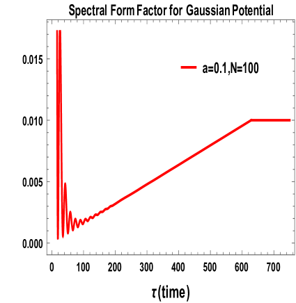
Refer to caption
(a) SFF for gaussian for a=.1,N=100formulae-sequence𝑎.1𝑁100a=.1,N=100
Refer to caption
(b) SFF for gaussian for a=.1,N=1000formulae-sequence𝑎.1𝑁1000a=.1,N=1000
Refer to caption
(c) SFF for gaussian for a=.1,N=10000formulae-sequence𝑎.1𝑁10000a=.1,N=10000
Figure 24: Time variation of SFF for different N at β=0𝛽0\beta=0. Here we used a scale factor SFF+0.01137𝑆𝐹𝐹0.01137SFF+0.01137

In fig. 24(a), fig. 24(b), fig. 24(c) it is observed that SFF with variation in N𝑁N get saturated at different value of τ𝜏\tau. But with increasing N𝑁N the value of the saturation point, will decrease. Subtracting the change of axis[SFF|τ=0evaluated-at𝑆𝐹𝐹𝜏0SFF|_{\tau=0}] we get the predicted bound of SFF.

5.5.2 For Quartic random potential

Here we consider quartic random potential which can be written as:

V(M)=12M2+gM4.𝑉𝑀12superscript𝑀2𝑔superscript𝑀4\displaystyle V(M)=\frac{1}{2}M^{2}+gM^{4}. (354)

For a single interval (n=1𝑛1n=1) with end points -2a and 2a (semi-circle) we get the following expression for density function for eigen value of the random matrix M𝑀M as given by:

ρ(λ)=1π4a2λ2(a1λ2+a0).𝜌𝜆1𝜋4superscript𝑎2superscript𝜆2subscript𝑎1superscript𝜆2subscript𝑎0\displaystyle\rho(\lambda)=\frac{1}{\pi}\sqrt{4a^{2}-\lambda^{2}}~{}\left(a_{1}\lambda^{2}+a_{0}\right). (355)

Now, for the quartic random potential ω(λ+i0)𝜔𝜆𝑖0\omega(\lambda+i0) can be expressed as:

ω(λ+i0)=12(2C2λ+4gλ3)+i4a2λ2(a1λ2+a0).𝜔𝜆𝑖0122subscript𝐶2𝜆4𝑔superscript𝜆3𝑖4superscript𝑎2superscript𝜆2subscript𝑎1superscript𝜆2subscript𝑎0\displaystyle\omega(\lambda+i0)=\frac{1}{2}\left(2C_{2}\lambda+4g\lambda^{3}\right)+i\sqrt{4a^{2}-\lambda^{2}}\left(a_{1}\lambda^{2}+a_{0}\right). (356)

Now Taylor expanding ω(λ+i0)𝜔𝜆𝑖0\omega(\lambda+i0) near λ𝜆\lambda\rightarrow\infty gives the following expression:

(2a1a2a0+12)λ+λ3(2ga1)+10a1a8+4a0a6λ52subscript𝑎1superscript𝑎2subscript𝑎012𝜆superscript𝜆32𝑔subscript𝑎110subscript𝑎1superscript𝑎84subscript𝑎0superscript𝑎6superscript𝜆5\displaystyle\left(2a_{1}a^{2}-a_{0}+\frac{1}{2}\right)\lambda+\lambda^{3}\left(2g-a_{1}\right)+\frac{10a_{1}a^{8}+4a_{0}a^{6}}{\lambda^{5}}
+4a1a6+2a0a4λ3+2a1a4+2a0a2λ+O((1λ)6)=1λ.4subscript𝑎1superscript𝑎62subscript𝑎0superscript𝑎4superscript𝜆32subscript𝑎1superscript𝑎42subscript𝑎0superscript𝑎2𝜆𝑂superscript1𝜆61𝜆\displaystyle~{}~{}~{}~{}~{}~{}~{}~{}~{}~{}~{}~{}~{}~{}~{}~{}~{}~{}~{}~{}~{}~{}+\frac{4a_{1}a^{6}+2a_{0}a^{4}}{\lambda^{3}}+\frac{2a_{1}a^{4}+2a_{0}a^{2}}{\lambda}+O\left(\left(\frac{1}{\lambda}\right)^{6}\right)=\frac{1}{\lambda}. (357)

Therefore equating both sides of the above equation gives:

a1=2g,subscript𝑎12𝑔\displaystyle a_{1}=2g, (358)
a0=4a2g+12,subscript𝑎04superscript𝑎2𝑔12\displaystyle a_{0}=4a^{2}g+\frac{1}{2}, (359)

along with the following constraint condition:

12ga4+a2=1.12𝑔superscript𝑎4superscript𝑎2112ga^{4}+a^{2}=1. (360)

Then the density function in terms of the eigen value of random matrix M𝑀M is given by the following expression:

ρ(λ)=1π(12+4ga2+2gλ2)4a2λ2.𝜌𝜆1𝜋124𝑔superscript𝑎22𝑔superscript𝜆24superscript𝑎2superscript𝜆2\displaystyle\rho(\lambda)=\frac{1}{\pi}\left(\frac{1}{2}+4ga^{2}+2g\lambda^{2}\right)~{}\sqrt{4a^{2}-\lambda^{2}}. (361)

Further solving the constraint we get:

a2=48g+1124g.superscript𝑎248𝑔1124𝑔\displaystyle a^{2}=\frac{\sqrt{48g+1}-1}{24g}. (362)

and Here a2superscript𝑎2a^{2} has imaginary value for g148𝑔148g\leqslant-\frac{1}{48} and the critical value is given by:

gc=148.subscript𝑔𝑐148\boxed{g_{c}=-\frac{1}{48}}~{}. (363)
Refer to caption
(a) ρ(λ)𝜌𝜆\rho(\lambda) for quartic potential for different g𝑔g.
Refer to caption
(b) ρ(λ)𝜌𝜆\rho(\lambda) for quartic potential for different g𝑔g.
Figure 25: Eigen value distribution curve of density function for quartic potential for different parameter values. Here we fix a=1𝑎1a=1.

In fig. 25(a) and fig. 25(b) density function ρ(λ)𝜌𝜆\rho(\lambda) for quartic potential is plotted with a=1𝑎1a=1. The curve follows from Eq. (361). When g=0𝑔0g=0 it matches with Wigner law. For g>0𝑔0g>0 the curve shows a plateau region whereas for g<0𝑔0g<0 it preserve the semicircular nature with minor deviation.The plateau region denotes the deviation from Wigner law even at very less effect of quartic term (as g𝑔g is chosen to be small). The plateau region though converge with semicircle at end point. At gc=148subscript𝑔𝑐148g_{c}=-\frac{1}{48} the curve deviates but converge to semicircle at end points where as for g<gc𝑔subscript𝑔𝑐g<g_{c} the curve never converge to semicircle one supporting its non-existence. (See eq. (363) for details.).

Now we will calculate the one point function of the partition function for quartic random potential, which is given by the following expression:

Z(β±iτ)delimited-⟨⟩𝑍plus-or-minus𝛽𝑖𝜏\displaystyle\langle Z(\beta\pm i\tau)\rangle =\displaystyle= 1π2a2a𝑑λ(12+4ga2+2gλ2)4a2λ2eiτλeβλ1𝜋superscriptsubscript2𝑎2𝑎differential-d𝜆124𝑔superscript𝑎22𝑔superscript𝜆24superscript𝑎2superscript𝜆2superscript𝑒minus-or-plusiτ𝜆superscript𝑒𝛽𝜆\displaystyle\frac{1}{\pi}\int_{-2a}^{2a}d\lambda~{}\left(\frac{1}{2}+4ga^{2}+2g\lambda^{2}\right)~{}\sqrt{4a^{2}-\lambda^{2}}~{}e^{\mp\text{i$\tau$}\lambda}~{}e^{-\beta\lambda} (364)
=\displaystyle= a(β±iτ)2[(24a2g+1)(β±iτ)I1(2a(β±iτ))24agI2(2a(β±iτ))],𝑎superscriptplus-or-minus𝛽𝑖𝜏2delimited-[]24superscript𝑎2𝑔1plus-or-minus𝛽𝑖𝜏subscript𝐼12𝑎plus-or-minus𝛽𝑖𝜏24𝑎𝑔subscript𝐼22𝑎plus-or-minus𝛽𝑖𝜏\displaystyle\frac{a}{(\beta\pm i\tau)^{2}}\left[\left(24a^{2}g+1\right)(\beta\pm i\tau)I_{1}(2a(\beta\pm i\tau))-24agI_{2}(2a(\beta\pm i\tau))\right],~{}~{}~{}~{}~{}~{}~{}~{}~{}~{}

where In(x)subscript𝐼𝑛𝑥I_{n}(x) is the modified Bessel function of first kind with order n𝑛n.

Further taking the high temperature limit we get the following simplified expression for the one point function:

[Z(β±iτ)]β=0subscriptdelimited-[]delimited-⟨⟩𝑍plus-or-minus𝛽𝑖𝜏𝛽0\displaystyle\left[\langle Z(\beta\pm i\tau)\rangle\right]_{\beta=0} =\displaystyle= 1π2a2a𝑑λ(12+4ga2+2gλ2)4a2λ2eiτλ1𝜋superscriptsubscript2𝑎2𝑎differential-d𝜆124𝑔superscript𝑎22𝑔superscript𝜆24superscript𝑎2superscript𝜆2superscript𝑒minus-or-plusiτ𝜆\displaystyle\frac{1}{\pi}\int_{-2a}^{2a}d\lambda~{}\left(\frac{1}{2}+4ga^{2}+2g\lambda^{2}\right)~{}\sqrt{4a^{2}-\lambda^{2}}~{}e^{\mp\text{i$\tau$}\lambda} (365)
=\displaystyle= aτ2[±(24a2g+1)τI1(±2aτ)24agI2(±2aτ)].𝑎superscript𝜏2delimited-[]plus-or-minus24superscript𝑎2𝑔1𝜏subscript𝐼1plus-or-minus2𝑎𝜏24𝑎𝑔subscript𝐼2plus-or-minus2𝑎𝜏\displaystyle\frac{a}{\text{$\tau$}^{2}}\left[\pm\left(24a^{2}g+1\right)\text{$\tau$}I_{1}(\pm 2a\text{$\tau$})-24agI_{2}(\pm 2a\text{$\tau$})\right].

Therefore the first term vanishes exactly at the critical point gc=148subscript𝑔𝑐148g_{c}=-\frac{1}{48} which gives:

a2=124gc=2.superscript𝑎2124subscript𝑔𝑐2\boxed{a^{2}=\frac{1}{24g_{c}}=2}~{}. (366)

Now taking the limit 𝒯=Nt𝒯𝑁𝑡{\cal T}=\sqrt{N}t\rightarrow\infty we get finally the following simplified result for the one point function:

[Z(β±i𝒯)]β=0subscriptdelimited-[]delimited-⟨⟩𝑍plus-or-minus𝛽𝑖𝒯𝛽0\displaystyle\left[\langle Z(\beta\pm i{\cal T})\rangle\right]_{\beta=0} =\displaystyle= 1(±𝒯)3/2aπ[(24a2g+1)cos(±2a𝒯+π4)±24gsin(±2a𝒯+π4)𝒯]1superscriptplus-or-minus𝒯32𝑎𝜋delimited-[]plus-or-minus24superscript𝑎2𝑔1plus-or-minus2𝑎𝒯𝜋424𝑔plus-or-minus2𝑎𝒯𝜋4𝒯\displaystyle-\frac{1}{(\pm{\cal T})^{3/2}}\sqrt{\frac{a}{\pi}}\left[\left(24a^{2}g+1\right)\cos\left(\pm 2a{\cal T}+\frac{\pi}{4}\right)\pm\frac{24g\sin\left(\pm 2a{\cal T}+\frac{\pi}{4}\right)}{{\cal T}}\right] (367)
+O(1(±𝒯)72).𝑂1superscriptplus-or-minus𝒯72\displaystyle~{}~{}~{}~{}~{}~{}~{}~{}~{}~{}~{}~{}~{}~{}~{}~{}~{}~{}~{}~{}~{}~{}~{}~{}~{}~{}~{}~{}~{}~{}~{}~{}~{}~{}~{}~{}~{}~{}~{}~{}~{}~{}~{}~{}~{}~{}~{}~{}~{}~{}~{}~{}~{}~{}~{}~{}~{}~{}~{}~{}~{}~{}~{}~{}+O\left(\frac{1}{(\pm{\cal T})^{\frac{7}{2}}}\right)~{}.~{}~{}~{}~{}~{}~{}~{}~{}~{}~{}~{}~{}~{}

Now for the quartic random potential disconnected part of the Green’s function can be computed at finite temperature as:

Gdc(β,τ)subscript𝐺𝑑𝑐𝛽𝜏\displaystyle G_{dc}(\beta,\tau) =\displaystyle= Z(β+iτ)Z(βiτ)Z(β)2delimited-⟨⟩𝑍𝛽𝑖𝜏delimited-⟨⟩𝑍𝛽𝑖𝜏superscriptdelimited-⟨⟩𝑍𝛽2\displaystyle\frac{\langle Z(\beta+i\tau)\rangle\langle Z(\beta-i\tau)\rangle}{\langle Z(\beta)\rangle^{2}} (368)
=\displaystyle= β4(β2+τ2)21[(24a2g+1)βI1(2aβ)24agI2(2aβ)]2superscript𝛽4superscriptsuperscript𝛽2superscript𝜏221superscriptdelimited-[]24superscript𝑎2𝑔1𝛽subscript𝐼12𝑎𝛽24𝑎𝑔subscript𝐼22𝑎𝛽2\displaystyle\frac{\beta^{4}}{(\beta^{2}+\tau^{2})^{2}}\frac{1}{\left[\left(24a^{2}g+1\right)\beta I_{1}(2a\beta)-24agI_{2}(2a\beta)\right]^{2}}
×[(24a2g+1)(β+iτ)I1(2a(β+iτ))24agI2(2a(β+iτ))]absentdelimited-[]24superscript𝑎2𝑔1𝛽𝑖𝜏subscript𝐼12𝑎𝛽𝑖𝜏24𝑎𝑔subscript𝐼22𝑎𝛽𝑖𝜏\displaystyle~{}~{}~{}~{}~{}~{}~{}~{}~{}~{}\times\left[\left(24a^{2}g+1\right)(\beta+i\tau)I_{1}(2a(\beta+i\tau))-24agI_{2}(2a(\beta+i\tau))\right]
×[(24a2g+1)(βiτ)I1(2a(βiτ))24agI2(2a(βiτ))],absentdelimited-[]24superscript𝑎2𝑔1𝛽𝑖𝜏subscript𝐼12𝑎𝛽𝑖𝜏24𝑎𝑔subscript𝐼22𝑎𝛽𝑖𝜏\displaystyle~{}~{}~{}~{}~{}~{}~{}~{}~{}~{}\times\left[\left(24a^{2}g+1\right)(\beta-i\tau)I_{1}(2a(\beta-i\tau))-24agI_{2}(2a(\beta-i\tau))\right],~{}~{}~{}~{}~{}~{}~{}~{}~{}~{}

which can be further simplified in the high temperature limiting situation as:

Gdc(τ)subscript𝐺𝑑𝑐𝜏\displaystyle G_{dc}(\tau) =\displaystyle= [Z(β+iτ)Z(βiτ)Z(β)2]β=0subscriptdelimited-[]delimited-⟨⟩𝑍𝛽𝑖𝜏delimited-⟨⟩𝑍𝛽𝑖𝜏superscriptdelimited-⟨⟩𝑍𝛽2𝛽0\displaystyle\left[\frac{\langle Z(\beta+i\tau)\rangle\langle Z(\beta-i\tau)\rangle}{\langle Z(\beta)\rangle^{2}}\right]_{\beta=0} (369)
=\displaystyle= a2N2τ4[(24a2g+1)(iτ)I1(2a(iτ))24agI2(2a(iτ))]superscript𝑎2superscript𝑁2superscript𝜏4delimited-[]24superscript𝑎2𝑔1𝑖𝜏subscript𝐼12𝑎𝑖𝜏24𝑎𝑔subscript𝐼22𝑎𝑖𝜏\displaystyle\frac{a^{2}}{N^{2}\tau^{4}}\left[\left(24a^{2}g+1\right)(i\tau)I_{1}(2a(i\tau))-24agI_{2}(2a(i\tau))\right]
×[(24a2g+1)(iτ)I1(2a(iτ))24agI2(2a(iτ))],.absentdelimited-[]24superscript𝑎2𝑔1𝑖𝜏subscript𝐼12𝑎𝑖𝜏24𝑎𝑔subscript𝐼22𝑎𝑖𝜏\displaystyle~{}~{}~{}~{}~{}~{}~{}~{}~{}~{}\times\left[\left(24a^{2}g+1\right)(-i\tau)I_{1}(2a(-i\tau))-24agI_{2}(2a(-i\tau))\right],~{}~{}~{}~{}~{}~{}~{}~{}~{}~{}.~{}~{}~{}~{}~{}~{}

Further taking the limit 𝒯=Nτ𝒯𝑁𝜏{\cal T}=\sqrt{N}\tau\rightarrow\infty we get the following simplified result:

Gdc(𝒯)subscript𝐺𝑑𝑐𝒯\displaystyle G_{dc}({\cal T}) =\displaystyle= [Z(β+i𝒯)Z(βi𝒯)Z(β)2]β=0subscriptdelimited-[]delimited-⟨⟩𝑍𝛽𝑖𝒯delimited-⟨⟩𝑍𝛽𝑖𝒯superscriptdelimited-⟨⟩𝑍𝛽2𝛽0\displaystyle\left[\frac{\langle Z(\beta+i{\cal T})\rangle\langle Z(\beta-i{\cal T})\rangle}{\langle Z(\beta)\rangle^{2}}\right]_{\beta=0} (370)
=\displaystyle= i𝒯3aN2π{[(24a2g+1)cos(2a𝒯+π4)+24gsin(2a𝒯+π4)𝒯]+O(1(𝒯)72)}𝑖superscript𝒯3𝑎superscript𝑁2𝜋delimited-[]24superscript𝑎2𝑔12𝑎𝒯𝜋424𝑔2𝑎𝒯𝜋4𝒯𝑂1superscript𝒯72\displaystyle\frac{i}{{\cal T}^{3}}{\frac{a}{N^{2}\pi}}\left\{\left[\left(24a^{2}g+1\right)\cos\left(2a{\cal T}+\frac{\pi}{4}\right)+\frac{24g\sin\left(2a{\cal T}+\frac{\pi}{4}\right)}{{\cal T}}\right]+O\left(\frac{1}{({\cal T})^{\frac{7}{2}}}\right)\right\}
×{[(24a2g+1)cos(2a𝒯π4)24gsin(2a𝒯π4)𝒯]+O(1(𝒯)72)}.absentdelimited-[]24superscript𝑎2𝑔12𝑎𝒯𝜋424𝑔2𝑎𝒯𝜋4𝒯𝑂1superscript𝒯72\displaystyle~{}~{}~{}~{}\times\left\{\left[\left(24a^{2}g+1\right)\cos\left(2a{\cal T}-\frac{\pi}{4}\right)-\frac{24g\sin\left(2a{\cal T}-\frac{\pi}{4}\right)}{{\cal T}}\right]+O\left(\frac{1}{(-{\cal T})^{\frac{7}{2}}}\right)\right\}.~{}~{}~{}~{}~{}~{}~{}~{}~{}~{}

Now to compute SFF we need to add both connected and disconnected part of the Green’s function G𝐺G(=Gc+Gdcabsentsubscript𝐺𝑐subscript𝐺𝑑𝑐=G_{c}+G_{dc}). Therefore, for quartic polynomial potential we get finally the following expression for SFF at finite temp:

𝐒𝐅𝐅(β,τ){β4(β2+τ2)21[(24a2g+1)βI1(2aβ)24agI2(2aβ)]2×[(24a2g+1)(β+iτ)I1(2a(β+iτ))24agI2(2a(β+iτ))]×[(24a2g+1)(βiτ)I1(2a(βiτ))24agI2(2a(βiτ))]+τ(2πN)21N+1(πN),τ<2πN β4(β2+τ2)21[(24a2g+1)βI1(2aβ)24agI2(2aβ)]2×[(24a2g+1)(β+iτ)I1(2a(β+iτ))24agI2(2a(β+iτ))]×[(24a2g+1)(βiτ)I1(2a(βiτ))24agI2(2a(βiτ))]+1πN,τ>2πN,𝐒𝐅𝐅𝛽𝜏casessuperscript𝛽4superscriptsuperscript𝛽2superscript𝜏221superscriptdelimited-[]24superscript𝑎2𝑔1𝛽subscript𝐼12𝑎𝛽24𝑎𝑔subscript𝐼22𝑎𝛽2missing-subexpressionmissing-subexpressionabsentdelimited-[]24superscript𝑎2𝑔1𝛽𝑖𝜏subscript𝐼12𝑎𝛽𝑖𝜏24𝑎𝑔subscript𝐼22𝑎𝛽𝑖𝜏missing-subexpressionmissing-subexpressionabsentdelimited-[]24superscript𝑎2𝑔1𝛽𝑖𝜏subscript𝐼12𝑎𝛽𝑖𝜏24𝑎𝑔subscript𝐼22𝑎𝛽𝑖𝜏missing-subexpressionmissing-subexpression𝜏superscript2𝜋𝑁21𝑁1𝜋𝑁τ<2πN missing-subexpressionmissing-subexpressionmissing-subexpressionmissing-subexpressionsuperscript𝛽4superscriptsuperscript𝛽2superscript𝜏221superscriptdelimited-[]24superscript𝑎2𝑔1𝛽subscript𝐼12𝑎𝛽24𝑎𝑔subscript𝐼22𝑎𝛽2missing-subexpressionmissing-subexpressionabsentdelimited-[]24superscript𝑎2𝑔1𝛽𝑖𝜏subscript𝐼12𝑎𝛽𝑖𝜏24𝑎𝑔subscript𝐼22𝑎𝛽𝑖𝜏missing-subexpressionmissing-subexpressionabsentdelimited-[]24superscript𝑎2𝑔1𝛽𝑖𝜏subscript𝐼12𝑎𝛽𝑖𝜏24𝑎𝑔subscript𝐼22𝑎𝛽𝑖𝜏missing-subexpressionmissing-subexpression1𝜋𝑁𝜏2𝜋𝑁missing-subexpressionmissing-subexpressionmissing-subexpression\boxed{\begin{array}[]{lll}\displaystyle{\bf SFF}(\beta,\tau)\equiv\left\{\begin{array}[]{lll}\displaystyle\frac{\beta^{4}}{(\beta^{2}+\tau^{2})^{2}}\frac{1}{\left[\left(24a^{2}g+1\right)\beta I_{1}(2a\beta)-24agI_{2}(2a\beta)\right]^{2}}\\ \displaystyle~{}~{}~{}~{}~{}~{}~{}~{}~{}~{}\times\left[\left(24a^{2}g+1\right)(\beta+i\tau)I_{1}(2a(\beta+i\tau))-24agI_{2}(2a(\beta+i\tau))\right]\\ \displaystyle~{}~{}~{}~{}~{}~{}~{}~{}~{}~{}\times\left[\left(24a^{2}g+1\right)(\beta-i\tau)I_{1}(2a(\beta-i\tau))-24agI_{2}(2a(\beta-i\tau))\right]\\ \displaystyle~{}~{}~{}~{}~{}~{}~{}~{}~{}~{}+\frac{\tau}{(2\pi N)^{2}}-\frac{1}{N}+\frac{1}{(\pi N)}\,,{}{}{}{}{}{}{}{}{}{}{}{}&\mbox{\small{\color[rgb]{1,0,0}\bf{$\tau<2\pi N$ }}}\\ \\ \displaystyle\frac{\beta^{4}}{(\beta^{2}+\tau^{2})^{2}}\frac{1}{\left[\left(24a^{2}g+1\right)\beta I_{1}(2a\beta)-24agI_{2}(2a\beta)\right]^{2}}\\ \displaystyle~{}~{}~{}~{}~{}~{}~{}~{}~{}~{}\times\left[\left(24a^{2}g+1\right)(\beta+i\tau)I_{1}(2a(\beta+i\tau))-24agI_{2}(2a(\beta+i\tau))\right]\\ \displaystyle~{}~{}~{}~{}~{}~{}~{}~{}~{}~{}\times\left[\left(24a^{2}g+1\right)(\beta-i\tau)I_{1}(2a(\beta-i\tau))-24agI_{2}(2a(\beta-i\tau))\right]\\ \displaystyle~{}~{}~{}~{}~{}~{}~{}~{}~{}~{}+\frac{1}{\pi N}\,,{}{}{}{}{}{}{}{}{}{}{}{}&\mbox{\small{\color[rgb]{1,0,0}\bf{$\tau>2\pi N$}}}\end{array}\right.\end{array}}~{}~{}, (371)

where 𝐒𝐅𝐅(β,τ)𝐒𝐅𝐅𝛽𝜏{\bf SFF}(\beta,\tau) is defined with proper normalization and in our prescription it gives the total Green’s function as mentioned above. Further simplifying the result for high temperature limit we get the following expression for SFF, as given by:

𝐒𝐅𝐅(τ){a2N2τ4[(24a2g+1)(iτ)I1(2a(iτ))24agI2(2a(iτ))]×[(24a2g+1)(iτ)I1(2a(iτ))24agI2(2a(iτ))]+τ(2πN)21N+1(πN),τ<2πN a2N2τ4[(24a2g+1)(iτ)I1(2a(iτ))24agI2(2a(iτ))]×[(24a2g+1)(iτ)I1(2a(iτ))24agI2(2a(iτ))]+1πN,τ>2πN,𝐒𝐅𝐅𝜏casessuperscript𝑎2superscript𝑁2superscript𝜏4delimited-[]24superscript𝑎2𝑔1𝑖𝜏subscript𝐼12𝑎𝑖𝜏24𝑎𝑔subscript𝐼22𝑎𝑖𝜏missing-subexpressionmissing-subexpressionabsentdelimited-[]24superscript𝑎2𝑔1𝑖𝜏subscript𝐼12𝑎𝑖𝜏24𝑎𝑔subscript𝐼22𝑎𝑖𝜏missing-subexpressionmissing-subexpression𝜏superscript2𝜋𝑁21𝑁1𝜋𝑁τ<2πN missing-subexpressionmissing-subexpressionmissing-subexpressionmissing-subexpressionsuperscript𝑎2superscript𝑁2superscript𝜏4delimited-[]24superscript𝑎2𝑔1𝑖𝜏subscript𝐼12𝑎𝑖𝜏24𝑎𝑔subscript𝐼22𝑎𝑖𝜏missing-subexpressionmissing-subexpressionabsentdelimited-[]24superscript𝑎2𝑔1𝑖𝜏subscript𝐼12𝑎𝑖𝜏24𝑎𝑔subscript𝐼22𝑎𝑖𝜏missing-subexpressionmissing-subexpression1𝜋𝑁𝜏2𝜋𝑁missing-subexpressionmissing-subexpressionmissing-subexpression\boxed{\begin{array}[]{lll}\displaystyle{\bf SFF}(\tau)\equiv\left\{\begin{array}[]{lll}\displaystyle\frac{a^{2}}{N^{2}\tau^{4}}\left[\left(24a^{2}g+1\right)(i\tau)I_{1}(2a(i\tau))-24agI_{2}(2a(i\tau))\right]\\ \displaystyle~{}~{}~{}~{}~{}~{}~{}~{}~{}~{}\times\left[\left(24a^{2}g+1\right)(-i\tau)I_{1}(2a(-i\tau))-24agI_{2}(2a(-i\tau))\right]\\ \displaystyle~{}~{}~{}~{}~{}~{}~{}~{}~{}~{}+\frac{\tau}{(2\pi N)^{2}}-\frac{1}{N}+\frac{1}{(\pi N)}\,,{}{}{}{}{}{}{}{}{}{}{}{}&\mbox{\small{\color[rgb]{1,0,0}\bf{$\tau<2\pi N$ }}}\\ \\ \displaystyle\frac{a^{2}}{N^{2}\tau^{4}}\left[\left(24a^{2}g+1\right)(i\tau)I_{1}(2a(i\tau))-24agI_{2}(2a(i\tau))\right]\\ \displaystyle~{}~{}~{}~{}~{}~{}~{}~{}~{}~{}\times\left[\left(24a^{2}g+1\right)(-i\tau)I_{1}(2a(-i\tau))-24agI_{2}(2a(-i\tau))\right]\\ \displaystyle~{}~{}~{}~{}~{}~{}~{}~{}~{}~{}+\frac{1}{\pi N}\,,{}{}{}{}{}{}{}{}{}{}{}{}&\mbox{\small{\color[rgb]{1,0,0}\bf{$\tau>2\pi N$}}}\end{array}\right.\end{array}}~{}~{}, (372)

Further taking the limit 𝒯=Nτ𝒯𝑁𝜏{\cal T}=\sqrt{N}\tau\rightarrow\infty we get the following simplified result for SFF:

𝐒𝐅𝐅(𝒯){i𝒯3aN2π{[(24a2g+1)cos(2a𝒯+π4)+24gsin(2a𝒯+π4)𝒯]+O(1(𝒯)72)}×{[(24a2g+1)cos(2a𝒯π4)24gsin(2a𝒯π4)𝒯]+O(1(𝒯)72)}+𝒯(2π)2N5/21N+1(πN),𝒯<2πN3/2 i𝒯3aN2π{[(24a2g+1)cos(2a𝒯+π4)+24gsin(2a𝒯+π4)𝒯]+O(1(𝒯)72)}×{[(24a2g+1)cos(2a𝒯π4)24gsin(2a𝒯π4)𝒯]+O(1(𝒯)72)}+1πN,𝒯>2πN3/2𝐒𝐅𝐅𝒯cases𝑖superscript𝒯3𝑎superscript𝑁2𝜋delimited-[]24superscript𝑎2𝑔12𝑎𝒯𝜋424𝑔2𝑎𝒯𝜋4𝒯𝑂1superscript𝒯72missing-subexpressionmissing-subexpressionabsentdelimited-[]24superscript𝑎2𝑔12𝑎𝒯𝜋424𝑔2𝑎𝒯𝜋4𝒯𝑂1superscript𝒯72missing-subexpressionmissing-subexpression𝒯superscript2𝜋2superscript𝑁521𝑁1𝜋𝑁𝒯<2πN3/2 missing-subexpressionmissing-subexpressionmissing-subexpressionmissing-subexpressionmissing-subexpressionmissing-subexpressionmissing-subexpression𝑖superscript𝒯3𝑎superscript𝑁2𝜋delimited-[]24superscript𝑎2𝑔12𝑎𝒯𝜋424𝑔2𝑎𝒯𝜋4𝒯𝑂1superscript𝒯72missing-subexpressionmissing-subexpressionabsentdelimited-[]24superscript𝑎2𝑔12𝑎𝒯𝜋424𝑔2𝑎𝒯𝜋4𝒯𝑂1superscript𝒯72missing-subexpressionmissing-subexpression1𝜋𝑁𝒯2𝜋superscript𝑁32missing-subexpressionmissing-subexpressionmissing-subexpression\displaystyle\boxed{\begin{array}[]{lll}\small\displaystyle{\bf SFF}({\cal T})\equiv\left\{\begin{array}[]{lll}\displaystyle\frac{i}{{\cal T}^{3}}{\frac{a}{N^{2}\pi}}\left\{\left[\left(24a^{2}g+1\right)\cos\left(2a{\cal T}+\frac{\pi}{4}\right)+\frac{24g\sin\left(2a{\cal T}+\frac{\pi}{4}\right)}{{\cal T}}\right]+O\left(\frac{1}{({\cal T})^{\frac{7}{2}}}\right)\right\}\\ \displaystyle~{}~{}~{}~{}\times\left\{\left[\left(24a^{2}g+1\right)\cos\left(2a{\cal T}-\frac{\pi}{4}\right)-\frac{24g\sin\left(2a{\cal T}-\frac{\pi}{4}\right)}{{\cal T}}\right]+O\left(\frac{1}{(-{\cal T})^{\frac{7}{2}}}\right)\right\}\\ \displaystyle~{}~{}~{}~{}~{}~{}~{}~{}~{}+\frac{{\cal T}}{(2\pi)^{2}N^{5/2}}-\frac{1}{N}+\frac{1}{(\pi N)}\,,{}{}{}{}{}{}{}{}{}{}{}{}&\mbox{\small{\color[rgb]{1,0,0}\bf{${\cal T}<2\pi N^{3/2}$ }}}\\ \\ \\ \displaystyle\frac{i}{{\cal T}^{3}}{\frac{a}{N^{2}\pi}}\left\{\left[\left(24a^{2}g+1\right)\cos\left(2a{\cal T}+\frac{\pi}{4}\right)+\frac{24g\sin\left(2a{\cal T}+\frac{\pi}{4}\right)}{{\cal T}}\right]+O\left(\frac{1}{({\cal T})^{\frac{7}{2}}}\right)\right\}\\ \displaystyle~{}~{}~{}~{}\times\left\{\left[\left(24a^{2}g+1\right)\cos\left(2a{\cal T}-\frac{\pi}{4}\right)-\frac{24g\sin\left(2a{\cal T}-\frac{\pi}{4}\right)}{{\cal T}}\right]+O\left(\frac{1}{(-{\cal T})^{\frac{7}{2}}}\right)\right\}\\ \displaystyle~{}~{}~{}~{}~{}~{}~{}~{}~{}+\frac{1}{\pi N}\,,{}{}{}{}{}{}{}{}{}{}{}{}&\mbox{\small{\color[rgb]{1,0,0}\bf{${\cal T}>2\pi N^{3/2}$}}}\end{array}\right.\end{array}} (382)

Further simplifying the result for high temperature limit we get the following expression for SFF, as given by:

𝐒𝐅𝐅(τ){a2N2τ4[(24a2g+1)(iτ)I1(2a(iτ))24agI2(2a(iτ))]×[(24a2g+1)(iτ)I1(2a(iτ))24agI2(2a(iτ))]+τ(2πN)21N+1(πN),τ<2πN a2N2τ4[(24a2g+1)(iτ)I1(2a(iτ))24agI2(2a(iτ))]×[(24a2g+1)(iτ)I1(2a(iτ))24agI2(2a(iτ))]+1πN,τ>2πN,𝐒𝐅𝐅𝜏casessuperscript𝑎2superscript𝑁2superscript𝜏4delimited-[]24superscript𝑎2𝑔1𝑖𝜏subscript𝐼12𝑎𝑖𝜏24𝑎𝑔subscript𝐼22𝑎𝑖𝜏missing-subexpressionmissing-subexpressionabsentdelimited-[]24superscript𝑎2𝑔1𝑖𝜏subscript𝐼12𝑎𝑖𝜏24𝑎𝑔subscript𝐼22𝑎𝑖𝜏missing-subexpressionmissing-subexpression𝜏superscript2𝜋𝑁21𝑁1𝜋𝑁τ<2πN missing-subexpressionmissing-subexpressionmissing-subexpressionmissing-subexpressionmissing-subexpressionmissing-subexpressionmissing-subexpressionsuperscript𝑎2superscript𝑁2superscript𝜏4delimited-[]24superscript𝑎2𝑔1𝑖𝜏subscript𝐼12𝑎𝑖𝜏24𝑎𝑔subscript𝐼22𝑎𝑖𝜏missing-subexpressionmissing-subexpressionabsentdelimited-[]24superscript𝑎2𝑔1𝑖𝜏subscript𝐼12𝑎𝑖𝜏24𝑎𝑔subscript𝐼22𝑎𝑖𝜏missing-subexpressionmissing-subexpression1𝜋𝑁𝜏2𝜋𝑁missing-subexpressionmissing-subexpressionmissing-subexpression\boxed{\begin{array}[]{lll}\displaystyle{\bf SFF}(\tau)\equiv\left\{\begin{array}[]{lll}\displaystyle\frac{a^{2}}{N^{2}\tau^{4}}\left[\left(24a^{2}g+1\right)(i\tau)I_{1}(2a(i\tau))-24agI_{2}(2a(i\tau))\right]\\ \displaystyle~{}~{}~{}~{}~{}~{}~{}~{}~{}~{}\times\left[\left(24a^{2}g+1\right)(-i\tau)I_{1}(2a(-i\tau))-24agI_{2}(2a(-i\tau))\right]\\ \displaystyle~{}~{}~{}~{}~{}~{}~{}~{}~{}~{}+\frac{\tau}{(2\pi N)^{2}}-\frac{1}{N}+\frac{1}{(\pi N)}\,,{}{}{}{}{}{}{}{}{}{}{}{}&\mbox{\small{\color[rgb]{1,0,0}\bf{$\tau<2\pi N$ }}}\\ \\ \\ \displaystyle\frac{a^{2}}{N^{2}\tau^{4}}\left[\left(24a^{2}g+1\right)(i\tau)I_{1}(2a(i\tau))-24agI_{2}(2a(i\tau))\right]\\ \displaystyle~{}~{}~{}~{}~{}~{}~{}~{}~{}~{}\times\left[\left(24a^{2}g+1\right)(-i\tau)I_{1}(2a(-i\tau))-24agI_{2}(2a(-i\tau))\right]\\ \displaystyle~{}~{}~{}~{}~{}~{}~{}~{}~{}~{}+\frac{1}{\pi N}\,,{}{}{}{}{}{}{}{}{}{}{}{}&\mbox{\small{\color[rgb]{1,0,0}\bf{$\tau>2\pi N$}}}\end{array}\right.\end{array}}~{}~{}, (384)
Refer to caption
(a) SFF for quartic potential at β=10𝛽10\beta=10.
Refer to caption
(b) SFF for quartic potential at β=100𝛽100\beta=100.
Figure 26: Spectral Form Factor for quartic potential at different finite temperature[β𝛽\beta] with N=1000𝑁1000N=1000 and a=0.1𝑎0.1a=0.1

From fig. 26(a) and fig. 26(b), we see that SFF at finite temperature decays with increasing τ𝜏\tau and reach zero. But with changing β𝛽\beta SFF values remains almost same initially (for higher β𝛽\beta or lower value of temperature).

From both the figures we have shown that SFF decays to zero for finite temperature.
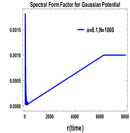
Refer to caption
(a) SFF for gaussian for a=.1,N=100formulae-sequence𝑎.1𝑁100a=.1,N=100 with SFF|τ=0=0.0068169evaluated-at𝑆𝐹𝐹𝜏00.0068169SFF|_{\tau=0}=0.0068169 as origin
Refer to caption
(b) SFF for gaussian for a=.1,N=1000formulae-sequence𝑎.1𝑁1000a=.1,N=1000 with SFF|τ=0=0.00068169evaluated-at𝑆𝐹𝐹𝜏00.00068169SFF|_{\tau=0}=0.00068169 as origin
Refer to caption
(c) SFF for gaussian for a=.1,N=10000formulae-sequence𝑎.1𝑁10000a=.1,N=10000 with SFF|τ=0=0.000068169evaluated-at𝑆𝐹𝐹𝜏00.000068169SFF|_{\tau=0}=0.000068169 as origin
Figure 27: Time variation of SFF for different N. Here we shift reference axis[SFF] to SFF|τ=0evaluated-at𝑆𝐹𝐹𝜏0SFF|_{\tau=0}

In fig. 27(a), fig. 27(b) and fig. 27(c), it is observed that SFF with variation in N𝑁N get saturated at different value of τ𝜏\tau. But with increasing N𝑁N the value of the saturation point, will decrease. Subtracting the change of axis[SFF|τ=0evaluated-at𝑆𝐹𝐹𝜏0SFF|_{\tau=0}] we get the predicted bound of SFF.

5.5.3 For Sextic random potential

In this subsection we consider sextic random potential, as given by the following expression:

V(M)=12M2+gM4+hM6.𝑉𝑀12superscript𝑀2𝑔superscript𝑀4superscript𝑀6\displaystyle V(M)=\frac{1}{2}M^{2}+gM^{4}+hM^{6}. (385)

For a single interval (n=1𝑛1n=1) with end points -2a and 2a (semi-circle) we get the following expression for the density function in terms of the eigen value of random matrix M𝑀M:

ρ(λ)=1π4a2λ2(a2λ4+a1λ2+a0).𝜌𝜆1𝜋4superscript𝑎2superscript𝜆2subscript𝑎2superscript𝜆4subscript𝑎1superscript𝜆2subscript𝑎0\displaystyle\rho(\lambda)=\frac{1}{\pi}~{}\sqrt{4a^{2}-\lambda^{2}}~{}\left(a_{2}\lambda^{4}+a_{1}\lambda^{2}+a_{0}\right). (386)

Also for sextic potential ω(λ+i0)𝜔𝜆𝑖0\omega(\lambda+i0) can be expressed as:

ω(λ+i0)=12(4gλ3+6hλ5+λ)+i4a2λ2(a2λ4+a1λ2+a0).𝜔𝜆𝑖0124𝑔superscript𝜆36superscript𝜆5𝜆𝑖4superscript𝑎2superscript𝜆2subscript𝑎2superscript𝜆4subscript𝑎1superscript𝜆2subscript𝑎0\displaystyle\omega(\lambda+i0)=\frac{1}{2}\left(4g\lambda^{3}+6h\lambda^{5}+\lambda\right)+i\sqrt{4a^{2}-\lambda^{2}}\left(a_{2}\lambda^{4}+a_{1}\lambda^{2}+a_{0}\right). (387)
Refer to caption
(a) ρ(λ)𝜌𝜆\rho(\lambda) for sextic potential for different g,h𝑔g,h.
Refer to caption
(b) ρ(λ)𝜌𝜆\rho(\lambda) for sextic potential for different g,h𝑔g,h.
Figure 28: Eigen value distribution curve of density function for sextic potential for different parameter values. Here we fix a=1𝑎1a=1.

In fig. 28(a) and fig. 28(b) for sextic potential behaviour of density function ρ(λ)𝜌𝜆\rho(\lambda) is shown. The curve follows from Eq. (392). Again choosing g=h=0𝑔0g=h=0 will produce the Wigner law. Deviating g𝑔g and hh by small amount shows deviation from Wigner semicircle law. For g>0,h>0formulae-sequence𝑔00g>0,h>0 the curve shows plateau region though merge with semicircle at end points. But choosing g<0,h<0formulae-sequence𝑔00g<0,h<0 and g=0𝑔0g=0 and h<00h<0 show deviation from semicircle and don’t converge even at end points.

Further expanding ω(λ+i0)𝜔𝜆𝑖0\omega(\lambda+i0) near λ𝜆\lambda\rightarrow\infty we get:

λ3(2a2a2a1+2g)superscript𝜆32subscript𝑎2superscript𝑎2subscript𝑎12𝑔\displaystyle\lambda^{3}\left(2a_{2}a^{2}-a_{1}+2g\right) +(2a2a4+2a1a2a0+12)λ2subscript𝑎2superscript𝑎42subscript𝑎1superscript𝑎2subscript𝑎012𝜆\displaystyle+\left(2a_{2}a^{4}+2a_{1}a^{2}-a_{0}+\frac{1}{2}\right)\lambda (388)
+4a2a6+2a1a4+2a0a2λ+λ5(3ha2)+O((1λ)3)=1λ.4subscript𝑎2superscript𝑎62subscript𝑎1superscript𝑎42subscript𝑎0superscript𝑎2𝜆superscript𝜆53subscript𝑎2𝑂superscript1𝜆31𝜆\displaystyle~{}~{}~{}~{}~{}~{}~{}+\frac{4a_{2}a^{6}+2a_{1}a^{4}+2a_{0}a^{2}}{\lambda}+\lambda^{5}\left(3h-a_{2}\right)+O\left(\left(\frac{1}{\lambda}\right)^{3}\right)=\frac{1}{\lambda}.~{}~{}~{}~{}~{}~{}~{}~{}~{}~{}~{}

Therefore, equating both the sides of the above equation we get:

a2subscript𝑎2\displaystyle a_{2} =\displaystyle= 3h,3\displaystyle 3h, (389)
a1subscript𝑎1\displaystyle a_{1} =\displaystyle= 2g+6a2h,2𝑔6superscript𝑎2\displaystyle 2g+6a^{2}h, (390)
a0subscript𝑎0\displaystyle a_{0} =\displaystyle= 18a4h+4a2g+12.18superscript𝑎44superscript𝑎2𝑔12\displaystyle 18a^{4}h+4a^{2}g+\frac{1}{2}. (391)

along with we get one additional constraint condition, as given by:

60a6h+12ga4+a2=160superscript𝑎612𝑔superscript𝑎4superscript𝑎2160a^{6}h+12ga^{4}+a^{2}=1

Then, for the sextic random potential we get the following simplified expression for the density function in terms of the eigen value of the random matrix M𝑀M, as given by:

ρ(λ)=1π4a2λ2(18a4h+λ2(6a2h+2g)+4a2g+3hλ4+12).𝜌𝜆1𝜋4superscript𝑎2superscript𝜆218superscript𝑎4superscript𝜆26superscript𝑎22𝑔4superscript𝑎2𝑔3superscript𝜆412\displaystyle\rho(\lambda)=\frac{1}{\pi}\sqrt{4a^{2}-\lambda^{2}}~{}\left(18a^{4}h+\lambda^{2}\left(6a^{2}h+2g\right)+4a^{2}g+3h\lambda^{4}+\frac{1}{2}\right). (392)

Solving the constraint condition we get, a2superscript𝑎2a^{2} in terms of g𝑔g and hh. The real root for a2superscript𝑎2a^{2} is given by the following expression:

a2=(g,h)30h180h144g21080h(g,h)g15h.superscript𝑎2𝑔30180144superscript𝑔21080𝑔𝑔15\displaystyle a^{2}=\frac{{\cal F}(g,h)}{30h}-\frac{180h-144g^{2}}{1080h{\cal F}(g,h)}-\frac{g}{15h}. (393)

where we define the function (g,h)𝑔{\cal F}(g,h) as:

(g,h)=8g3+5144g3h23g2h2+270gh3+2025h4+5h3+15gh+225h23.𝑔38superscript𝑔35144superscript𝑔3superscript23superscript𝑔2superscript2270𝑔superscript32025superscript45superscript315𝑔225superscript2\displaystyle{\cal F}(g,h)=\sqrt[3]{-8g^{3}+5\sqrt{-144g^{3}h^{2}-3g^{2}h^{2}+270gh^{3}+2025h^{4}+5h^{3}}+15gh+225h^{2}}.~{}~{}~{}~{}~{}~{}~{}~{}~{}~{} (394)

Here we can check that putting h=00h=0 the constraint condition reduces to the following simplified form:

12ga4+a2=112𝑔superscript𝑎4superscript𝑎2112ga^{4}+a^{2}=1 (395)

and the solution of this equation is given by the following expression:

a2=48g+1124g.superscript𝑎248𝑔1124𝑔\boxed{a^{2}=\frac{\sqrt{48g+1}-1}{24g}}. (396)

Here the critical value with h=00h=0 is given by:

gc=148,subscript𝑔𝑐148\boxed{g_{c}=-\frac{1}{48}}~{}, (397)

which is exactly same result as obtained for quartic potential in the previous subsection.

Now the expression for the one point function for partition function at finite temperature can be computed as:

Z(β±iτ)delimited-⟨⟩𝑍plus-or-minus𝛽𝑖𝜏\displaystyle\langle Z(\beta\pm i\tau)\rangle =\displaystyle= 1π2a2a𝑑λ4a2λ2(18a4h+λ2(6a2h+2g)+4a2g+3hλ4+12)eiτλeβλ1𝜋superscriptsubscript2𝑎2𝑎differential-d𝜆4superscript𝑎2superscript𝜆218superscript𝑎4superscript𝜆26superscript𝑎22𝑔4superscript𝑎2𝑔3superscript𝜆412superscript𝑒minus-or-plus𝑖𝜏𝜆superscript𝑒𝛽𝜆\displaystyle\frac{1}{\pi}\int_{-2a}^{2a}d\lambda~{}\sqrt{4a^{2}-\lambda^{2}}\left(18a^{4}h+\lambda^{2}\left(6a^{2}h+2g\right)+4a^{2}g+3h\lambda^{4}+\frac{1}{2}\right)~{}e^{\mp i\tau\lambda}~{}e^{-\beta\lambda} (398)
=\displaystyle= a(β±iτ)4[(β±iτ)I1(2a(β±iτ))\displaystyle\frac{a}{(\beta\pm i\tau)^{4}}\left[(\beta\pm i\tau)I_{1}(2a(\beta\pm i\tau))\right.
(360a2h+β2(180a4h+24a2g+1)±2iβτ(180a4h+24a2g+1)\displaystyle\left.\left(360a^{2}h+\beta^{2}\left(180a^{4}h+24a^{2}g+1\right)\pm 2i\beta\tau\left(180a^{4}h+24a^{2}g+1\right)\right.\right.
τ2(180a4h+24a2g+1))\displaystyle\left.\left.-\tau^{2}\left(180a^{4}h+24a^{2}g+1\right)\right)\right.
24aI2(2a(β±iτ))(30h+(β±iτ)2(15a2h+g))]\displaystyle\left.-24aI_{2}(2a(\beta\pm i\tau))\left(30h+(\beta\pm i\tau)^{2}\left(15a^{2}h+g\right)\right)\right]

Further in the high temperature limit the one point function for partition function can be simplified as:

[Z(β±it)]β=0subscriptdelimited-[]delimited-⟨⟩𝑍plus-or-minus𝛽𝑖𝑡𝛽0\displaystyle\left[\langle Z(\beta\pm it)\rangle\right]_{\beta=0} =\displaystyle= 1π2a2a𝑑λ4a2λ2(18a4h+λ2(6a2h+2g)+4a2g+3hλ4+12)eiτλ1𝜋superscriptsubscript2𝑎2𝑎differential-d𝜆4superscript𝑎2superscript𝜆218superscript𝑎4superscript𝜆26superscript𝑎22𝑔4superscript𝑎2𝑔3superscript𝜆412superscript𝑒minus-or-plus𝑖𝜏𝜆\displaystyle\frac{1}{\pi}\int_{-2a}^{2a}d\lambda~{}\sqrt{4a^{2}-\lambda^{2}}\left(18a^{4}h+\lambda^{2}\left(6a^{2}h+2g\right)+4a^{2}g+3h\lambda^{4}+\frac{1}{2}\right)~{}e^{\mp i\tau\lambda} (399)
=\displaystyle= aτ4[(J1(±2aτ)((±τ)3(180a4h+24a2g+1)360a2hτ)\displaystyle\frac{a}{\tau^{4}}\left[(J_{1}(\pm 2a\tau)((\pm\tau)^{3}(180a^{4}h+24a^{2}g+1)\mp 360a^{2}h\tau)\right.
24J2(±2aτ)(τ2(15a2h+g)30h))]\displaystyle\left.\displaystyle~{}~{}~{}~{}~{}~{}~{}~{}~{}~{}~{}~{}~{}~{}~{}~{}~{}~{}~{}~{}~{}~{}-24J_{2}(\pm 2a\tau)(\tau^{2}(15a^{2}h+g)-30h))\right]

Next, simplifying the result for one point function in the limit 𝒯=Nτ𝒯𝑁𝜏{\cal T}=\sqrt{N}\tau\rightarrow\infty we get:

[Z(β±i𝒯)]β=0subscriptdelimited-[]delimited-⟨⟩𝑍plus-or-minus𝛽𝑖𝒯𝛽0\displaystyle\left[\langle Z(\beta\pm i{\cal T})\rangle\right]_{\beta=0} =\displaystyle= aπ1(±𝒯)32[(1+24a2g+180a4h)cos(π4±2a𝒯)\displaystyle\sqrt{\frac{a}{\pi}}\frac{1}{(\pm{\cal T})^{\frac{3}{2}}}\left[-\left(1+24a^{2}g+180a^{4}h\right)\cos\left(\frac{\pi}{4}\pm 2a{\cal T}\right)\right. (400)
±24ag+15a2h𝒯sin(π4±2a𝒯)plus-or-minus24𝑎𝑔15superscript𝑎2𝒯plus-or-minus𝜋42𝑎𝒯\displaystyle\left.~{}~{}~{}~{}~{}~{}~{}~{}\pm 24a\frac{g+15a^{2}h}{{\cal T}}\sin\left(\frac{\pi}{4}\pm 2a{\cal T}\right)\right.
+360a2h𝒯2cos(π4±2a𝒯)+O(1𝒯4)]\displaystyle\left.~{}~{}~{}~{}~{}~{}~{}~{}+\frac{360a^{2}h}{{\cal T}^{2}}\cos\left(\frac{\pi}{4}\pm 2a{\cal T}\right)+O\left(\frac{1}{{\cal T}^{4}}\right)\right]

Now for the quadratic random potential disconnected part of the Green’s function can be computed at finite temperature as:

Gdc(β,τ)subscript𝐺𝑑𝑐𝛽𝜏\displaystyle G_{dc}(\beta,\tau) =\displaystyle= Z(β+iτ)Z(βiτ)Z(β)2delimited-⟨⟩𝑍𝛽𝑖𝜏delimited-⟨⟩𝑍𝛽𝑖𝜏superscriptdelimited-⟨⟩𝑍𝛽2\displaystyle\frac{\langle Z(\beta+i\tau)\rangle\langle Z(\beta-i\tau)\rangle}{\langle Z(\beta)\rangle^{2}} (401)
=\displaystyle= β8(β2+τ2)4[βI1(2aβ)(360a2h+β2(180a4h+24a2g+1))\displaystyle\frac{\beta^{8}}{(\beta^{2}+\tau^{2})^{4}}\left[\beta I_{1}(2a\beta)\left(360a^{2}h+\beta^{2}\left(180a^{4}h+24a^{2}g+1\right)\right)\right.
24aI2(2aβ)(30h+β2(15a2h+g))]2\displaystyle\left.-24aI_{2}(2a\beta)\left(30h+\beta^{2}\left(15a^{2}h+g\right)\right)\right]^{-2}
×[(β+iτ)I1(2a(β+iτ))\displaystyle\times\left[(\beta+i\tau)I_{1}(2a(\beta+i\tau))\right.
(360a2h+β2(180a4h+24a2g+1)+2iβτ(180a4h+24a2g+1)\displaystyle\left.\left(360a^{2}h+\beta^{2}\left(180a^{4}h+24a^{2}g+1\right)+2i\beta\tau\left(180a^{4}h+24a^{2}g+1\right)\right.\right.
τ2(180a4h+24a2g+1))\displaystyle\left.\left.-\tau^{2}\left(180a^{4}h+24a^{2}g+1\right)\right)\right.
24aI2(2a(β+iτ))(30h+(β+iτ)2(15a2h+g))]\displaystyle\left.-24aI_{2}(2a(\beta+i\tau))\left(30h+(\beta+i\tau)^{2}\left(15a^{2}h+g\right)\right)\right]
×[(βiτ)I1(2a(βiτ))\displaystyle~{}~{}~{}~{}\times\left[(\beta-i\tau)I_{1}(2a(\beta-i\tau))\right.
(360a2h+β2(180a4h+24a2g+1)2iβτ(180a4h+24a2g+1)\displaystyle\left.\left(360a^{2}h+\beta^{2}\left(180a^{4}h+24a^{2}g+1\right)-2i\beta\tau\left(180a^{4}h+24a^{2}g+1\right)\right.\right.
τ2(180a4h+24a2g+1))\displaystyle\left.\left.-\tau^{2}\left(180a^{4}h+24a^{2}g+1\right)\right)\right.
24aI2(2a(βiτ))(30h+(βiτ)2(15a2h+g))],\displaystyle\left.-24aI_{2}(2a(\beta-i\tau))\left(30h+(\beta-i\tau)^{2}\left(15a^{2}h+g\right)\right)\right],~{}~{}~{}~{}~{}~{}

which can be further simplified in the high temperature limiting situation as:

Gdc(τ)subscript𝐺𝑑𝑐𝜏\displaystyle G_{dc}(\tau) =\displaystyle= [Z(β+iτ)Z(βiτ)Z(β)2]β=0subscriptdelimited-[]delimited-⟨⟩𝑍𝛽𝑖𝜏delimited-⟨⟩𝑍𝛽𝑖𝜏superscriptdelimited-⟨⟩𝑍𝛽2𝛽0\displaystyle\left[\frac{\langle Z(\beta+i\tau)\rangle\langle Z(\beta-i\tau)\rangle}{\langle Z(\beta)\rangle^{2}}\right]_{\beta=0} (402)
=\displaystyle= a2N2τ8[(J1(2aτ)(τ3(180a4h+24a2g+1)360a2hτ)\displaystyle\frac{a^{2}}{N^{2}\tau^{8}}\left[(J_{1}(2a\tau)(\tau^{3}(180a^{4}h+24a^{2}g+1)-360a^{2}h\tau)\right.
24J2(2aτ)(τ2(15a2h+g)30h))]\displaystyle\left.\displaystyle~{}~{}~{}~{}~{}~{}~{}~{}~{}~{}~{}~{}~{}~{}~{}~{}~{}~{}~{}~{}~{}~{}-24J_{2}(2a\tau)(\tau^{2}(15a^{2}h+g)-30h))\right]
×[(J1(2aτ)((τ)3(180a4h+24a2g+1)+360a2hτ)\displaystyle\times\left[(J_{1}(-2a\tau)((-\tau)^{3}(180a^{4}h+24a^{2}g+1)+360a^{2}h\tau)\right.
24J2(2aτ)(τ2(15a2h+g)30h))].\displaystyle\left.\displaystyle~{}~{}~{}~{}~{}~{}~{}~{}~{}~{}~{}~{}~{}~{}~{}~{}~{}~{}~{}~{}~{}~{}-24J_{2}(-2a\tau)(\tau^{2}(15a^{2}h+g)-30h))\right].~{}~{}~{}~{}~{}~{}

Further taking the limit 𝒯=Nτ𝒯𝑁𝜏{\cal T}=\sqrt{N}\tau\rightarrow\infty we get the following simplified result:

Gdc(𝒯)subscript𝐺𝑑𝑐𝒯\displaystyle G_{dc}({\cal T}) =\displaystyle= [Z(β+i𝒯)Z(βi𝒯)Z(β)2]β=0subscriptdelimited-[]delimited-⟨⟩𝑍𝛽𝑖𝒯delimited-⟨⟩𝑍𝛽𝑖𝒯superscriptdelimited-⟨⟩𝑍𝛽2𝛽0\displaystyle\left[\frac{\langle Z(\beta+i{\cal T})\rangle\langle Z(\beta-i{\cal T})\rangle}{\langle Z(\beta)\rangle^{2}}\right]_{\beta=0} (403)
=\displaystyle= i𝒯3aN2π[(1+24a2g+180a4h)cos(π4+2a𝒯)\displaystyle\frac{i}{{\cal T}^{3}}\frac{a}{N^{2}\pi}\left[-\left(1+24a^{2}g+180a^{4}h\right)\cos\left(\frac{\pi}{4}+2a{\cal T}\right)\right.
+24ag+15a2h𝒯sin(π4+2a𝒯)+360a2h𝒯2cos(π4+2a𝒯)+O(1𝒯4)]\displaystyle\left.~{}~{}~{}~{}~{}~{}~{}~{}+24a\frac{g+15a^{2}h}{{\cal T}}\sin\left(\frac{\pi}{4}+2a{\cal T}\right)+\frac{360a^{2}h}{{\cal T}^{2}}\cos\left(\frac{\pi}{4}+2a{\cal T}\right)+O\left(\frac{1}{{\cal T}^{4}}\right)\right]
×[(1+24a2g+180a4h)cos(π42a𝒯)\displaystyle\times\left[-\left(1+24a^{2}g+180a^{4}h\right)\cos\left(\frac{\pi}{4}-2a{\cal T}\right)\right.
24ag+15a2h𝒯sin(π42a𝒯)+360a2h𝒯2cos(π42a𝒯)+O(1𝒯4)].\displaystyle\left.~{}~{}~{}~{}~{}~{}~{}~{}-24a\frac{g+15a^{2}h}{{\cal T}}\sin\left(\frac{\pi}{4}-2a{\cal T}\right)+\frac{360a^{2}h}{{\cal T}^{2}}\cos\left(\frac{\pi}{4}-2a{\cal T}\right)+O\left(\frac{1}{{\cal T}^{4}}\right)\right].~{}~{}~{}~{}~{}~{}~{}~{}~{}~{}

Now to compute SFF we need to add both connected and disconnected part of the Green’s function G𝐺G(=Gc+Gdcabsentsubscript𝐺𝑐subscript𝐺𝑑𝑐=G_{c}+G_{dc}). Therefore, for sextic polynomial potential we get finally the following expression for SFF at finite temp:

𝐒𝐅𝐅(β,τ)β8(β2+τ2)4[βI1(2aβ)(360a2h+β2(180a4h+24a2g+1))24aI2(2aβ)(30h+β2(15a2h+g))]2[(β+iτ)I1(2a(β+iτ))(360a2h+β2(180a4h+24a2g+1)+2iβτ(180a4h+24a2g+1)τ2(180a4h+24a2g+1))24aI2(2a(β+iτ))(30h+(β+iτ)2(15a2h+g))]×[(βiτ)I1(2a(βiτ))(360a2h+β2(180a4h+24a2g+1)2iβτ(180a4h+24a2g+1)τ2(180a4h+24a2g+1))24aI2(2a(βiτ))(30h+(βiτ)2(15a2h+g))]+{τ(2πN)21N+1(πN),τ<2πN 1πN,τ>2πN\displaystyle\boxed{\begin{array}[]{lll}\footnotesize{\bf SFF}(\beta,\tau)&\equiv&\displaystyle\frac{\beta^{8}}{(\beta^{2}+\tau^{2})^{4}}\left[\beta I_{1}(2a\beta)\left(360a^{2}h+\beta^{2}\left(180a^{4}h+24a^{2}g+1\right)\right)\right.\\ &&\left.-24aI_{2}(2a\beta)\left(30h+\beta^{2}\left(15a^{2}h+g\right)\right)\right]^{-2}\left[(\beta+i\tau)I_{1}(2a(\beta+i\tau))\right.\\ &&\left.\left(360a^{2}h+\beta^{2}\left(180a^{4}h+24a^{2}g+1\right)+2i\beta\tau\left(180a^{4}h+24a^{2}g+1\right)\right.\right.\\ &&\left.\left.-\tau^{2}\left(180a^{4}h+24a^{2}g+1\right)\right)-24aI_{2}(2a(\beta+i\tau))\left(30h+(\beta+i\tau)^{2}\left(15a^{2}h+g\right)\right)\right]\\ &&~{}~{}~{}~{}\times\left[(\beta-i\tau)I_{1}(2a(\beta-i\tau))\right.\\ &&\left.\left(360a^{2}h+\beta^{2}\left(180a^{4}h+24a^{2}g+1\right)-2i\beta\tau\left(180a^{4}h+24a^{2}g+1\right)\right.\right.\\ &&\left.\left.-\tau^{2}\left(180a^{4}h+24a^{2}g+1\right)\right)-24aI_{2}(2a(\beta-i\tau))\left(30h+(\beta-i\tau)^{2}\left(15a^{2}h+g\right)\right)\right]\\ &&~{}~{}~{}+\left\{\begin{array}[]{lll}\displaystyle\frac{\tau}{(2\pi N)^{2}}-\frac{1}{N}+\frac{1}{(\pi N)}\,,{}{}{}{}{}{}{}{}{}{}{}{}&\mbox{\small{\color[rgb]{1,0,0}\bf{$\tau<2\pi N$ }}}\\ \displaystyle\frac{1}{\pi N}\,,{}{}{}{}{}{}{}{}{}{}{}{}&\mbox{\small{\color[rgb]{1,0,0}\bf{$\tau>2\pi N$}}}\end{array}\right.\end{array}}~{}~{}~{}~{}~{}~{}~{} (414)

where 𝐒𝐅𝐅(β,τ)𝐒𝐅𝐅𝛽𝜏{\bf SFF}(\beta,\tau) is defined with proper normalization and in our prescription it gives the total Green’s function as mentioned above.

Further simplifying the result for high temperature limit we get the following expression for SFF, as given by:

𝐒𝐅𝐅(τ)a2N2τ8[(J1(2aτ)(τ3(180a4h+24a2g+1)360a2hτ)24J2(2aτ)(τ2(15a2h+g)30h))]×[(J1(2aτ)((τ)3(180a4h+24a2g+1)+360a2hτ)24J2(2aτ)(τ2(15a2h+g)30h))]+{τ(2πN)21N+1(πN),τ<2πN 1πN,τ>2πN\displaystyle\boxed{\begin{array}[]{lll}{\bf SFF}(\tau)&\equiv&\displaystyle\frac{a^{2}}{N^{2}\tau^{8}}\left[(J_{1}(2a\tau)(\tau^{3}(180a^{4}h+24a^{2}g+1)-360a^{2}h\tau)\right.\\ &&\left.\displaystyle~{}~{}~{}~{}~{}~{}~{}~{}~{}~{}~{}~{}~{}~{}~{}~{}~{}~{}~{}~{}~{}~{}-24J_{2}(2a\tau)(\tau^{2}(15a^{2}h+g)-30h))\right]\\ &&\times\left[(J_{1}(-2a\tau)((-\tau)^{3}(180a^{4}h+24a^{2}g+1)+360a^{2}h\tau)\right.\\ &&\left.\displaystyle~{}~{}~{}~{}~{}~{}~{}~{}~{}~{}~{}~{}~{}~{}~{}~{}~{}~{}~{}~{}~{}~{}-24J_{2}(-2a\tau)(\tau^{2}(15a^{2}h+g)-30h))\right]\\ &&+\left\{\begin{array}[]{lll}\displaystyle\frac{\tau}{(2\pi N)^{2}}-\frac{1}{N}+\frac{1}{(\pi N)}\,,{}{}{}{}{}{}{}{}{}{}{}{}&\mbox{\small{\color[rgb]{1,0,0}\bf{$\tau<2\pi N$ }}}\\ \displaystyle\frac{1}{\pi N}\,,{}{}{}{}{}{}{}{}{}{}{}{}&\mbox{\small{\color[rgb]{1,0,0}\bf{$\tau>2\pi N$}}}\end{array}\right.\end{array}}~{}~{}~{}~{}~{}~{}~{}~{} (422)

Further taking the limit 𝒯=Nτ𝒯𝑁𝜏{\cal T}=\sqrt{N}\tau\rightarrow\infty we get the following simplified result for SFF:

𝐒𝐅𝐅(𝒯)i𝒯3aN2π[(1+24a2g+180a4h)cos(π4+2a𝒯)+24ag+15a2h𝒯sin(π4+2a𝒯)+360a2h𝒯2cos(π4+2a𝒯)+O(1𝒯4)]×[(1+24a2g+180a4h)cos(π42a𝒯)24ag+15a2h𝒯sin(π42a𝒯)+360a2h𝒯2cos(π42a𝒯)+O(1𝒯4)]+{𝒯(2π)2N5/21N+1(πN),𝒯<2πN3/2 1πN,𝒯>2πN3/2\displaystyle\boxed{\begin{array}[]{lll}{\bf SFF}({\cal T})&\equiv&\displaystyle\frac{i}{{\cal T}^{3}}\frac{a}{N^{2}\pi}\left[-\left(1+24a^{2}g+180a^{4}h\right)\cos\left(\frac{\pi}{4}+2a{\cal T}\right)\right.\\ &&\left.~{}~{}~{}~{}~{}~{}~{}~{}+24a\frac{g+15a^{2}h}{{\cal T}}\sin\left(\frac{\pi}{4}+2a{\cal T}\right)+\frac{360a^{2}h}{{\cal T}^{2}}\cos\left(\frac{\pi}{4}+2a{\cal T}\right)+O\left(\frac{1}{{\cal T}^{4}}\right)\right]\\ &&\times\left[-\left(1+24a^{2}g+180a^{4}h\right)\cos\left(\frac{\pi}{4}-2a{\cal T}\right)\right.\\ &&\left.~{}~{}~{}~{}~{}~{}~{}~{}-24a\frac{g+15a^{2}h}{{\cal T}}\sin\left(\frac{\pi}{4}-2a{\cal T}\right)+\frac{360a^{2}h}{{\cal T}^{2}}\cos\left(\frac{\pi}{4}-2a{\cal T}\right)+O\left(\frac{1}{{\cal T}^{4}}\right)\right]\\ &&+\left\{\begin{array}[]{lll}\displaystyle\frac{{\cal T}}{(2\pi)^{2}N^{5/2}}-\frac{1}{N}+\frac{1}{(\pi N)}\,,{}{}{}{}{}{}{}{}{}{}{}{}&\mbox{\small{\color[rgb]{1,0,0}\bf{${\cal T}<2\pi N^{3/2}$ }}}\\ \displaystyle\frac{1}{\pi N}\,,{}{}{}{}{}{}{}{}{}{}{}{}&\mbox{\small{\color[rgb]{1,0,0}\bf{${\cal T}>2\pi N^{3/2}$}}}\end{array}\right.\end{array}}~{}~{}~{}~{}~{} (430)
Refer to caption
(a) SFF for sextic potential at β=10𝛽10\beta=10.
Refer to caption
(b) SFF for sextic potential at β=100𝛽100\beta=100.
Figure 29: Spectral Form Factor for sextic potential at different finite temperature[β𝛽\beta] with N=1000𝑁1000N=1000 and a=0.1𝑎0.1a=0.1

From fig. 29(a) and fig. 29(b), we see that SFF at finite temperature decays with increasing τ𝜏\tau and reach zero. But with changing β𝛽\beta SFF values remains almost same initially (for higher β𝛽\beta).

Refer to caption
(a) SFF for sextic for a=.1,N=100formulae-sequence𝑎.1𝑁100a=.1,N=100 with SFF|τ=0=0.0068169evaluated-at𝑆𝐹𝐹𝜏00.0068169SFF|_{\tau=0}=0.0068169 as origin.
Refer to caption
(b) SFF for sextic for a=.1,N=1000formulae-sequence𝑎.1𝑁1000a=.1,N=1000 with SFF|τ=0=0.00068169evaluated-at𝑆𝐹𝐹𝜏00.00068169SFF|_{\tau=0}=0.00068169 as origin
Refer to caption
(c) SFF for sextic for a=.1,N=10000formulae-sequence𝑎.1𝑁10000a=.1,N=10000 with SFF|τ=0=0.000068169evaluated-at𝑆𝐹𝐹𝜏00.000068169SFF|_{\tau=0}=0.000068169 as origin
Figure 30: Time variation of SFF for different N at β=0𝛽0\beta=0.Here we shift reference axis[SFF] to SFF|τ=0evaluated-at𝑆𝐹𝐹𝜏0SFF|_{\tau=0}

In fig. 30(a), fig. 30(b), fig. 30(c), it is observed that SFF with variation in N𝑁N get saturated at different value of τ𝜏\tau. But with increasing N𝑁N the value of the saturation point, will decrease. Subtracting the change of axis[SFF|τ=0evaluated-at𝑆𝐹𝐹𝜏0SFF|_{\tau=0}] we get the predicted bound of SFF.

5.5.4 For Octa random potential

Here we consider octa random potential, as given by the following expression:

V(M)=12M2+gM4+hM6+kM8.𝑉𝑀12superscript𝑀2𝑔superscript𝑀4superscript𝑀6𝑘superscript𝑀8\displaystyle V(M)=\frac{1}{2}M^{2}+gM^{4}+hM^{6}+kM^{8}. (431)

For a single interval (n=1𝑛1n=1) with end points -2a and 2a (semi-circle) we get the following expression for the density function in terms of the eigen value of the random matrix M𝑀M, as given by:

ρ(λ)=1π4a2λ2(a3λ6+a2λ4+a1λ2+a0).𝜌𝜆1𝜋4superscript𝑎2superscript𝜆2subscript𝑎3superscript𝜆6subscript𝑎2superscript𝜆4subscript𝑎1superscript𝜆2subscript𝑎0\displaystyle\rho(\lambda)=\frac{1}{\pi}\sqrt{4a^{2}-\lambda^{2}}~{}\left(a_{3}\lambda^{6}+a_{2}\lambda^{4}+a_{1}\lambda^{2}+a_{0}\right). (432)

Then the function ω(λ+i0)𝜔𝜆𝑖0\omega(\lambda+i0) can be expressed as:

ω(λ+i0)=12(4gλ3+6hλ5+8kλ7+λ)+i4a2λ2(a3λ6+a2λ4+a1λ2+a0).𝜔𝜆𝑖0124𝑔superscript𝜆36superscript𝜆58𝑘superscript𝜆7𝜆𝑖4superscript𝑎2superscript𝜆2subscript𝑎3superscript𝜆6subscript𝑎2superscript𝜆4subscript𝑎1superscript𝜆2subscript𝑎0\displaystyle\omega(\lambda+i0)=\frac{1}{2}\left(4g\lambda^{3}+6h\lambda^{5}+8k\lambda^{7}+\lambda\right)+i\sqrt{4a^{2}-\lambda^{2}}\left(a_{3}\lambda^{6}+a_{2}\lambda^{4}+a_{1}\lambda^{2}+a_{0}\right). (433)

Further Taylor expanding ω(λ+i0)𝜔𝜆𝑖0\omega(\lambda+i0) near λ𝜆\lambda\rightarrow\infty we get:

λ5(2a3a2a2+3h)superscript𝜆52subscript𝑎3superscript𝑎2subscript𝑎23\displaystyle\lambda^{5}\left(2a_{3}a^{2}-a_{2}+3h\right) +λ3(2a3a4+2a2a2a1+2g)+(4a3a6+2a2a4+2a1a2a0+12)λsuperscript𝜆32subscript𝑎3superscript𝑎42subscript𝑎2superscript𝑎2subscript𝑎12𝑔4subscript𝑎3superscript𝑎62subscript𝑎2superscript𝑎42subscript𝑎1superscript𝑎2subscript𝑎012𝜆\displaystyle+\lambda^{3}\left(2a_{3}a^{4}+2a_{2}a^{2}-a_{1}+2g\right)+\left(4a_{3}a^{6}+2a_{2}a^{4}+2a_{1}a^{2}-a_{0}+\frac{1}{2}\right)\lambda (434)
+10a3a8+4a2a6+2a1a4+2a0a2λ+λ7(4ka3)+O((1λ)3)=1λ.10subscript𝑎3superscript𝑎84subscript𝑎2superscript𝑎62subscript𝑎1superscript𝑎42subscript𝑎0superscript𝑎2𝜆superscript𝜆74𝑘subscript𝑎3𝑂superscript1𝜆31𝜆\displaystyle+\frac{10a_{3}a^{8}+4a_{2}a^{6}+2a_{1}a^{4}+2a_{0}a^{2}}{\lambda}+\lambda^{7}\left(4k-a_{3}\right)+O\left(\left(\frac{1}{\lambda}\right)^{3}\right)=\frac{1}{\lambda}.~{}~{}~{}~{}~{}~{}~{}~{}~{}~{}~{}

Therefore, equating both the sides of the above equation we get:

a3subscript𝑎3\displaystyle a_{3} =\displaystyle= 4k,4𝑘\displaystyle 4k, (435)
a2subscript𝑎2\displaystyle a_{2} =\displaystyle= 3h+8a2k,38superscript𝑎2𝑘\displaystyle 3h+8a^{2}k, (436)
a1subscript𝑎1\displaystyle a_{1} =\displaystyle= 24a4k+6a2h+2g,24superscript𝑎4𝑘6superscript𝑎22𝑔\displaystyle 24a^{4}k+6a^{2}h+2g, (437)
a0subscript𝑎0\displaystyle a_{0} =\displaystyle= 12(160a6k+36a4h+8a2g+1),12160superscript𝑎6𝑘36superscript𝑎48superscript𝑎2𝑔1\displaystyle\frac{1}{2}\left(160a^{6}k+36a^{4}h+8a^{2}g+1\right), (438)

along with an additional constraint condition:

a2+12a4g+60a6h+280a8k=1superscript𝑎212superscript𝑎4𝑔60superscript𝑎6280superscript𝑎8𝑘1a^{2}+12a^{4}g+60a^{6}h+280a^{8}k=1 (439)

Solution of this constraint equation gives a2superscript𝑎2a^{2} in terms of g𝑔g, hh and k𝑘k. Since the solutions for a2superscript𝑎2a^{2} are very complicated, we have not explicitly mentioned them here. Instead of writing full solution here we can check that putting h=00h=0 the constraint condition reduces to the following simplified form:

12ga4+a2=112𝑔superscript𝑎4superscript𝑎2112ga^{4}+a^{2}=1 (440)

and the solution of this equation is given by the following expression:

a2=48g+1124g.superscript𝑎248𝑔1124𝑔\boxed{a^{2}=\frac{\sqrt{48g+1}-1}{24g}}~{}. (441)

Here the critical value with h=00h=0 and k=0𝑘0k=0 is given by the following expression:

gc=148,subscript𝑔𝑐148\boxed{g_{c}=-\frac{1}{48}}~{}, (442)

which is exactly same result as obtained for quartic and sextic (with h=00h=0) potential in the previous subsections.

Then, the final expression for the density function in terms of the eigen value of the random matrix M𝑀M can be written as:

ρ(λ)𝜌𝜆\displaystyle\rho(\lambda) =\displaystyle= 1π4a2λ2(80a6k+6a4(3h+4kλ2)+a2(4g+6hλ2+8kλ4)\displaystyle\frac{1}{\pi}\sqrt{4a^{2}-\lambda^{2}}~{}\left(80a^{6}k+6a^{4}\left(3h+4k\lambda^{2}\right)+a^{2}\left(4g+6h\lambda^{2}+8k\lambda^{4}\right)\right. (443)
+2gλ2+3hλ4+4kλ6+12).\displaystyle\left.~{}~{}~{}~{}~{}~{}~{}~{}~{}~{}~{}~{}~{}~{}~{}~{}~{}~{}~{}~{}~{}~{}~{}~{}~{}~{}~{}~{}~{}~{}~{}~{}~{}~{}~{}~{}~{}~{}~{}~{}~{}~{}~{}+2g\lambda^{2}+3h\lambda^{4}+4k\lambda^{6}+\frac{1}{2}\right).~{}~{}~{}~{}~{}~{}
Refer to caption
(a) ρ(λ)𝜌𝜆\rho(\lambda) for octa potential for different g,h,k
Refer to caption
(b) ρ(λ)𝜌𝜆\rho(\lambda) for octa potential for different g,h,k
Figure 31: Eigen value distribution curve of density function for quartic and octa potential for different parameter values. Here we fix a=1𝑎1a=1.

In fig. 31(a) and fig. 31(b) for octic potential behaviour of density function ρ(λ)𝜌𝜆\rho(\lambda) is shown. The curve follows from Eq. (443). Again choosing g=h=k=0𝑔𝑘0g=h=k=0 will produce the Wigner law. Deviating g𝑔g, hh and k𝑘k by small amount shows deviation from Wigner semicircle law. For g=0,h>0,k>0formulae-sequence𝑔0formulae-sequence0𝑘0g=0,h>0,k>0 the curve shows plateau region though merge with semicircle at end points. But choosing g>0,h<0,k<0formulae-sequence𝑔0formulae-sequence0𝑘0g>0,h<0,k<0 and g>0,h>0,k<0formulae-sequence𝑔0formulae-sequence0𝑘0g>0,h>0,k<0 show deviation from semicircle and don’t converge even at end points. On the other hand, if we choose g>0,h>0,k>0formulae-sequence𝑔0formulae-sequence0𝑘0g>0,h>0,k>0 then we get a valley region lying between two peaks of the maxima of the density distribution of eigen values of the random matrices under consideration. The same behaviour can be obtained by fixing g>0,h<0,k>0formulae-sequence𝑔0formulae-sequence0𝑘0g>0,h<0,k>0, g=h=k=1𝑔𝑘1g=h=k=1 and g=0,h>>0,k>>0formulae-sequence𝑔0formulae-sequencemuch-greater-than0much-greater-than𝑘0g=0,h>>0,k>>0. Only slight difference can be visualised in the peak heights of the maxima and also in the spread in the valley region. But in all such cases in between it will not at all match with the Wigner semicircle law, but converge to the end points of the Wigner semi-circle , which is obtained by setting g=h=k=0𝑔𝑘0g=h=k=0.

Next, we compute the expression for the one point function of the partition function at finite temperature, which can be expressed as:

Z(β±iτ)delimited-⟨⟩𝑍plus-or-minus𝛽𝑖𝜏\displaystyle\displaystyle\langle Z(\beta\pm i\tau)\rangle =\displaystyle= 1π2a2adλ4a2λ2(80a6k+6a4(3h+4kλ2)+a2(4g+6hλ2+8kλ4)\displaystyle\frac{1}{\pi}\int_{-2a}^{2a}d\lambda~{}\sqrt{4a^{2}-\lambda^{2}}~{}\left(80a^{6}k+6a^{4}\left(3h+4k\lambda^{2}\right)+a^{2}\left(4g+6h\lambda^{2}+8k\lambda^{4}\right)\right.
+2gλ2+3hλ4+4kλ6+12)eiτλeβλ\displaystyle\left.~{}~{}~{}~{}~{}~{}~{}~{}~{}~{}~{}~{}~{}~{}~{}~{}~{}~{}~{}~{}~{}~{}~{}~{}~{}~{}~{}~{}~{}+2g\lambda^{2}+3h\lambda^{4}+4k\lambda^{6}+\frac{1}{2}\right)~{}e^{\mp i\tau\lambda}~{}e^{-\beta\lambda}
=\displaystyle= 1(β±iτ)6[24a2I2(2(β±iτ)|a|)(15a2hτ4+β4(140a4k+15a2h+g)\displaystyle\frac{1}{(\beta\pm i\tau)^{6}}\left[-24a^{2}I_{2}(2(\beta\pm i\tau)\left|a\right|)\left(15a^{2}h\tau^{4}+\beta^{4}\left(140a^{4}k+15a^{2}h+g\right)\right.\right.
±4iβ3τ(140a4k+15a2h+g)6β2(140a4kτ2+5h(3a2τ21)140a2k+gτ2)plus-or-minus4𝑖superscript𝛽3𝜏140superscript𝑎4𝑘15superscript𝑎2𝑔6superscript𝛽2140superscript𝑎4𝑘superscript𝜏253superscript𝑎2superscript𝜏21140superscript𝑎2𝑘𝑔superscript𝜏2\displaystyle\left.\left.~{}~{}\pm 4i\beta^{3}\tau\left(140a^{4}k+15a^{2}h+g\right)-6\beta^{2}\left(140a^{4}k\tau^{2}+5h\left(3a^{2}\tau^{2}-1\right)-140a^{2}k+g\tau^{2}\right)\right.\right.
4iβτ(140a4kτ2+15h(a2τ21)420a2k+gτ2)minus-or-plus4𝑖𝛽𝜏140superscript𝑎4𝑘superscript𝜏215superscript𝑎2superscript𝜏21420superscript𝑎2𝑘𝑔superscript𝜏2\displaystyle\left.\left.~{}~{}\mp 4i\beta\tau\left(140a^{4}k\tau^{2}+15h\left(a^{2}\tau^{2}-1\right)-420a^{2}k+g\tau^{2}\right)\right.\right.
+140k(a4τ46a2τ2+12)+gτ430hτ2)\displaystyle\left.\left.~{}~{}~{}~{}~{}~{}~{}~{}~{}~{}~{}~{}~{}~{}~{}~{}~{}~{}~{}~{}+140k\left(a^{4}\tau^{4}-6a^{2}\tau^{2}+12\right)+g\tau^{4}-30h\tau^{2}\right)\right.
+|a|(β±iτ)3I1(2(β±iτ)|a|)(1120a6kτ2+60a4(112k3hτ2)\displaystyle\left.~{}~{}~{}~{}~{}~{}~{}~{}~{}~{}~{}~{}~{}~{}~{}~{}~{}~{}~{}~{}+\left|a\right|(\beta\pm i\tau)^{3}I_{1}(2(\beta\pm i\tau)\left|a\right|)\left(-1120a^{6}k\tau^{2}+60a^{4}\left(112k-3h\tau^{2}\right)\right.\right.
+24a2(15hgτ2)+β2(1120a6k+180a4h+24a2g+1)24superscript𝑎215𝑔superscript𝜏2superscript𝛽21120superscript𝑎6𝑘180superscript𝑎424superscript𝑎2𝑔1\displaystyle\left.\left.~{}~{}~{}~{}~{}~{}~{}~{}~{}~{}~{}~{}~{}~{}~{}~{}~{}~{}~{}~{}+24a^{2}\left(15h-g\tau^{2}\right)+\beta^{2}\left(1120a^{6}k+180a^{4}h+24a^{2}g+1\right)\right.\right.
±2iβτ(1120a6k+180a4h+24a2g+1)τ2)+20160k|a|3(β±iτ)I1(2(β±iτ)|a|)],\displaystyle\left.\left.\pm 2i\beta\tau\left(1120a^{6}k+180a^{4}h+24a^{2}g+1\right)-\tau^{2}\right)+20160k\left|a\right|^{3}(\beta\pm i\tau)I_{1}(2(\beta\pm i\tau)\left|a\right|)\right],

where In(x)subscript𝐼𝑛𝑥I_{n}(x) is the modified Bessel function of first kind with n𝑛n th order.

Further, considering the high temperature limiting situation we get the following simplified expression for the one point function of the partition function:

[Z(β±iτ)]β=0subscriptdelimited-[]delimited-⟨⟩𝑍plus-or-minus𝛽𝑖𝜏𝛽0\displaystyle\displaystyle\left[\langle Z(\beta\pm i\tau)\rangle\right]_{\beta=0} =\displaystyle= 1π2a2adλ4a2λ2(80a6k+6a4(3h+4kλ2)+a2(4g+6hλ2+8kλ4)\displaystyle\frac{1}{\pi}\int_{-2a}^{2a}d\lambda~{}\sqrt{4a^{2}-\lambda^{2}}~{}\left(80a^{6}k+6a^{4}\left(3h+4k\lambda^{2}\right)+a^{2}\left(4g+6h\lambda^{2}+8k\lambda^{4}\right)\right. (445)
+2gλ2+3hλ4+4kλ6+12)eiτλ\displaystyle\left.~{}~{}~{}~{}~{}~{}~{}~{}~{}~{}~{}~{}~{}~{}~{}~{}~{}~{}~{}~{}~{}~{}~{}~{}~{}~{}~{}~{}~{}+2g\lambda^{2}+3h\lambda^{4}+4k\lambda^{6}+\frac{1}{2}\right)~{}e^{\mp i\tau\lambda}
=\displaystyle= aτ6[±J1(±2aτ)(1120a6kτ5+60a4τ3(3hτ2112k)\displaystyle\frac{a}{\tau^{6}}\left[\pm J_{1}(\pm 2a\tau)(1120a^{6}k\tau^{5}+60a^{4}\tau^{3}(3h\tau^{2}-112k)\right.
+24a2(gτ515hτ3+840kτ)+τ5)\displaystyle\left.+24a^{2}(g\tau^{5}-15h\tau^{3}+840k\tau)+\tau^{5})\right.
24J2(±2aτ)(30τ2(28a2k+h)+τ4(140a4k+15a2h+g)+1680k)].\displaystyle\left.\displaystyle-24J_{2}(\pm 2a\tau)(-30\tau^{2}(28a^{2}k+h)+\tau^{4}(140a^{4}k+15a^{2}h+g)+1680k)\right].~{}~{}~{}~{}~{}~{}~{}~{}~{}~{}~{}~{}~{}~{}

Next, simplifying the result for one point function in the limit 𝒯=Nτ𝒯𝑁𝜏{\cal T}=\sqrt{N}\tau\rightarrow\infty we get:

[Z(β±i𝒯)]β=0subscriptdelimited-[]delimited-⟨⟩𝑍plus-or-minus𝛽𝑖𝒯𝛽0\displaystyle\left[\langle Z(\beta\pm i{\cal T})\rangle\right]_{\beta=0} =aπ1(±𝒯)32[(1120a6k+180a4h+2a2g+1\displaystyle=\sqrt{\frac{a}{\pi}}\frac{1}{(\pm{\cal T})^{\frac{3}{2}}}\left[\left(1120a^{6}k+180a^{4}h+2a^{2}g+1\right.\right. (446)
(6720a4k+360a2h𝒯2))cos(π4±2a𝒯)\displaystyle\left.\left.\displaystyle~{}~{}~{}~{}~{}~{}~{}~{}-\left(\frac{6720a^{4}k+360a^{2}h}{{\cal T}^{2}}\right)\right)\cos\left(\frac{\pi}{4}\pm 2a{\cal T}\right)\right.
24(140a4k+15a2h+g𝒯(840a2k+30h𝒯3))sin(π4±2a𝒯)]\displaystyle\left.\displaystyle~{}~{}~{}~{}~{}~{}~{}~{}\mp 24\left(\frac{140a^{4}k+15a^{2}h+g}{{\cal T}}-\left(\frac{840a^{2}k+30h}{{\cal T}^{3}}\right)\right)\sin\left(\frac{\pi}{4}\pm 2a{\cal T}\right)\right]
+O(1(±𝒯)112).𝑂1superscriptplus-or-minus𝒯112\displaystyle~{}~{}~{}~{}~{}~{}~{}~{}~{}~{}~{}~{}~{}+O\left(\frac{1}{(\pm{\cal T})^{\frac{11}{2}}}\right).

Now for the octic random potential disconnected part of the Green’s function can be computed at finite temperature as:

Gdc(β,τ)subscript𝐺𝑑𝑐𝛽𝜏\displaystyle G_{dc}(\beta,\tau) =\displaystyle= Z(β+iτ)Z(βiτ)Z(β)2=β12(β2+τ2)6[24a2I2(2β|a|)\displaystyle\frac{\langle Z(\beta+i\tau)\rangle\langle Z(\beta-i\tau)\rangle}{\langle Z(\beta)\rangle^{2}}=\frac{\beta^{12}}{(\beta^{2}+\tau^{2})^{6}}\left[-24a^{2}I_{2}(2\beta\left|a\right|)\right. (447)
(β4(140a4k+15a2h+g)+6β2(5h+140a2k)+1680k)superscript𝛽4140superscript𝑎4𝑘15superscript𝑎2𝑔6superscript𝛽25140superscript𝑎2𝑘1680𝑘\displaystyle\left.~{}~{}~{}~{}~{}~{}~{}~{}~{}~{}~{}~{}~{}~{}~{}~{}~{}~{}~{}~{}\left(\beta^{4}\left(140a^{4}k+15a^{2}h+g\right)+6\beta^{2}\left(5h+140a^{2}k\right)+1680k\right)\right.
+|a|β3I1(2(β)|a|)(6720a4k+360a2h\displaystyle\left.~{}~{}~{}~{}~{}~{}~{}~{}~{}~{}~{}~{}~{}~{}~{}~{}~{}~{}~{}~{}+\left|a\right|\beta^{3}I_{1}(2(\beta)\left|a\right|)\left(6720a^{4}k+360a^{2}h\right.\right.
+β2(1120a6k+180a4h+24a2g+1))+20160k|a|3βI1(2(β)|a|)]2\displaystyle\left.\left.~{}~{}~{}~{}~{}~{}~{}~{}~{}~{}~{}~{}~{}~{}~{}~{}~{}~{}~{}~{}+\beta^{2}\left(1120a^{6}k+180a^{4}h+24a^{2}g+1\right)\right)+20160k\left|a\right|^{3}\beta I_{1}(2(\beta)\left|a\right|)\right]^{-2}
×[24a2I2(2(β+iτ)|a|)\displaystyle~{}~{}~{}~{}~{}\times\left[-24a^{2}I_{2}(2(\beta+i\tau)\left|a\right|)\right.
(15a2hτ4+β4(140a4k+15a2h+g)\displaystyle\left.~{}~{}~{}~{}~{}~{}~{}~{}~{}~{}~{}~{}~{}~{}~{}~{}~{}~{}~{}~{}\left(15a^{2}h\tau^{4}+\beta^{4}\left(140a^{4}k+15a^{2}h+g\right)\right.\right.
+4iβ3τ(140a4k+15a2h+g)4𝑖superscript𝛽3𝜏140superscript𝑎4𝑘15superscript𝑎2𝑔\displaystyle\left.\left.~{}~{}~{}~{}~{}~{}~{}~{}~{}~{}~{}~{}~{}~{}~{}~{}~{}~{}~{}~{}+4i\beta^{3}\tau\left(140a^{4}k+15a^{2}h+g\right)\right.\right.
6β2(140a4kτ2+5h(3a2τ21)140a2k+gτ2)6superscript𝛽2140superscript𝑎4𝑘superscript𝜏253superscript𝑎2superscript𝜏21140superscript𝑎2𝑘𝑔superscript𝜏2\displaystyle\left.\left.~{}~{}~{}~{}~{}~{}~{}~{}~{}~{}~{}~{}~{}~{}~{}~{}~{}~{}~{}~{}-6\beta^{2}\left(140a^{4}k\tau^{2}+5h\left(3a^{2}\tau^{2}-1\right)-140a^{2}k+g\tau^{2}\right)\right.\right.
4iβτ(140a4kτ2+15h(a2τ21)420a2k+gτ2)4𝑖𝛽𝜏140superscript𝑎4𝑘superscript𝜏215superscript𝑎2superscript𝜏21420superscript𝑎2𝑘𝑔superscript𝜏2\displaystyle\left.\left.~{}~{}~{}~{}~{}~{}~{}~{}~{}~{}~{}~{}~{}~{}~{}~{}~{}~{}~{}~{}-4i\beta\tau\left(140a^{4}k\tau^{2}+15h\left(a^{2}\tau^{2}-1\right)-420a^{2}k+g\tau^{2}\right)\right.\right.
+140k(a4τ46a2τ2+12)+gτ430hτ2)\displaystyle\left.\left.~{}~{}~{}~{}~{}~{}~{}~{}~{}~{}~{}~{}~{}~{}~{}~{}~{}~{}~{}~{}+140k\left(a^{4}\tau^{4}-6a^{2}\tau^{2}+12\right)+g\tau^{4}-30h\tau^{2}\right)\right.
+|a|(β+iτ)3I1(2(β+iτ)|a|)𝑎superscript𝛽𝑖𝜏3subscript𝐼12𝛽𝑖𝜏𝑎\displaystyle\left.~{}~{}~{}~{}~{}~{}~{}~{}~{}~{}~{}~{}~{}~{}~{}~{}~{}~{}~{}~{}+\left|a\right|(\beta+i\tau)^{3}I_{1}(2(\beta+i\tau)\left|a\right|)\right.
(1120a6kτ2+60a4(112k3hτ2)\displaystyle\left.~{}~{}~{}~{}~{}~{}~{}~{}~{}~{}~{}~{}~{}~{}~{}~{}~{}~{}~{}~{}\left(-1120a^{6}k\tau^{2}+60a^{4}\left(112k-3h\tau^{2}\right)\right.\right.
+24a2(15hgτ2)+β2(1120a6k+180a4h+24a2g+1)24superscript𝑎215𝑔superscript𝜏2superscript𝛽21120superscript𝑎6𝑘180superscript𝑎424superscript𝑎2𝑔1\displaystyle\left.\left.~{}~{}~{}~{}~{}~{}~{}~{}~{}~{}~{}~{}~{}~{}~{}~{}~{}~{}~{}~{}+24a^{2}\left(15h-g\tau^{2}\right)+\beta^{2}\left(1120a^{6}k+180a^{4}h+24a^{2}g+1\right)\right.\right.
+2iβτ(1120a6k+180a4h+24a2g+1)τ2)\displaystyle\left.\left.~{}~{}~{}~{}~{}~{}~{}~{}~{}~{}~{}~{}~{}~{}~{}~{}~{}~{}~{}~{}+2i\beta\tau\left(1120a^{6}k+180a^{4}h+24a^{2}g+1\right)-\tau^{2}\right)\right.
+20160k|a|3(β+iτ)I1(2(β+iτ)|a|)]\displaystyle\left.~{}~{}~{}~{}~{}~{}~{}~{}~{}~{}~{}~{}~{}~{}~{}~{}~{}~{}~{}~{}+20160k\left|a\right|^{3}(\beta+i\tau)I_{1}(2(\beta+i\tau)\left|a\right|)\right]
×[24a2I2(2(βiτ)|a|)\displaystyle~{}~{}~{}~{}~{}~{}~{}~{}~{}~{}~{}~{}~{}~{}\times\left[-24a^{2}I_{2}(2(\beta-i\tau)\left|a\right|)\right.
(15a2hτ4+β4(140a4k+15a2h+g)4iβ3τ(140a4k+15a2h+g)\displaystyle\left.~{}~{}~{}~{}~{}~{}~{}~{}~{}~{}~{}~{}~{}~{}~{}~{}~{}~{}~{}~{}\left(15a^{2}h\tau^{4}+\beta^{4}\left(140a^{4}k+15a^{2}h+g\right)-4i\beta^{3}\tau\left(140a^{4}k+15a^{2}h+g\right)\right.\right.
6β2(140a4kτ2+5h(3a2τ21)140a2k+gτ2)6superscript𝛽2140superscript𝑎4𝑘superscript𝜏253superscript𝑎2superscript𝜏21140superscript𝑎2𝑘𝑔superscript𝜏2\displaystyle\left.\left.~{}~{}~{}~{}~{}~{}~{}~{}~{}~{}~{}~{}~{}~{}~{}~{}~{}~{}~{}~{}-6\beta^{2}\left(140a^{4}k\tau^{2}+5h\left(3a^{2}\tau^{2}-1\right)-140a^{2}k+g\tau^{2}\right)\right.\right.
+4iβτ(140a4kτ2+15h(a2τ21)420a2k+gτ2)4𝑖𝛽𝜏140superscript𝑎4𝑘superscript𝜏215superscript𝑎2superscript𝜏21420superscript𝑎2𝑘𝑔superscript𝜏2\displaystyle\left.\left.~{}~{}~{}~{}~{}~{}~{}~{}~{}~{}~{}~{}~{}~{}~{}~{}~{}~{}~{}~{}+4i\beta\tau\left(140a^{4}k\tau^{2}+15h\left(a^{2}\tau^{2}-1\right)-420a^{2}k+g\tau^{2}\right)\right.\right.
+140k(a4τ46a2τ2+12)+gτ430hτ2)\displaystyle\left.\left.~{}~{}~{}~{}~{}~{}~{}~{}~{}~{}~{}~{}~{}~{}~{}~{}~{}~{}~{}~{}+140k\left(a^{4}\tau^{4}-6a^{2}\tau^{2}+12\right)+g\tau^{4}-30h\tau^{2}\right)\right.
+|a|(βiτ)3I1(2(βiτ)|a|)𝑎superscript𝛽𝑖𝜏3subscript𝐼12𝛽𝑖𝜏𝑎\displaystyle\left.~{}~{}~{}~{}~{}~{}~{}~{}~{}~{}~{}~{}~{}~{}~{}~{}~{}~{}~{}~{}+\left|a\right|(\beta-i\tau)^{3}I_{1}(2(\beta-i\tau)\left|a\right|)\right.
(1120a6kτ2+60a4(112k3hτ2)\displaystyle\left.~{}~{}~{}~{}~{}~{}~{}~{}~{}~{}~{}~{}~{}~{}~{}~{}~{}~{}~{}~{}\left(-1120a^{6}k\tau^{2}+60a^{4}\left(112k-3h\tau^{2}\right)\right.\right.
24a2(15hgτ2)+β2(1120a6k+180a4h+24a2g+1)24superscript𝑎215𝑔superscript𝜏2superscript𝛽21120superscript𝑎6𝑘180superscript𝑎424superscript𝑎2𝑔1\displaystyle\left.\left.~{}~{}~{}~{}~{}~{}~{}~{}~{}~{}~{}~{}~{}~{}~{}~{}~{}~{}~{}~{}-24a^{2}\left(15h-g\tau^{2}\right)+\beta^{2}\left(1120a^{6}k+180a^{4}h+24a^{2}g+1\right)\right.\right.
2iβτ(1120a6k+180a4h+24a2g+1)τ2)\displaystyle\left.\left.~{}~{}~{}~{}~{}~{}~{}~{}~{}~{}~{}~{}~{}~{}~{}~{}~{}~{}~{}~{}-2i\beta\tau\left(1120a^{6}k+180a^{4}h+24a^{2}g+1\right)-\tau^{2}\right)\right.
+20160k|a|3(βiτ)I1(2(βiτ)|a|)]\displaystyle\left.~{}~{}~{}~{}~{}~{}~{}~{}~{}~{}~{}~{}~{}~{}~{}~{}~{}~{}~{}~{}+20160k\left|a\right|^{3}(\beta-i\tau)I_{1}(2(\beta-i\tau)\left|a\right|)\right]~{}~{}~{}~{}~{}~{}

which can be further simplified in the high temperature limiting situation as:

Gdc(τ)subscript𝐺𝑑𝑐𝜏\displaystyle G_{dc}(\tau) =\displaystyle= [Z(β+iτ)Z(βiτ)Z(β)2]β=0subscriptdelimited-[]delimited-⟨⟩𝑍𝛽𝑖𝜏delimited-⟨⟩𝑍𝛽𝑖𝜏superscriptdelimited-⟨⟩𝑍𝛽2𝛽0\displaystyle\left[\frac{\langle Z(\beta+i\tau)\rangle\langle Z(\beta-i\tau)\rangle}{\langle Z(\beta)\rangle^{2}}\right]_{\beta=0} (448)
=\displaystyle= a2N2τ12superscript𝑎2superscript𝑁2superscript𝜏12\displaystyle\frac{a^{2}}{N^{2}\tau^{12}}
×[J1(2aτ)(1120a6kτ5+60a4τ3(3hτ2112k)\displaystyle~{}~{}~{}~{}\times\ \left[J_{1}(2a\tau)(1120a^{6}k\tau^{5}+60a^{4}\tau^{3}(3h\tau^{2}-112k)\right.
+24a2(gτ515hτ3+840kτ)+τ5)\displaystyle\left.\displaystyle~{}~{}~{}~{}~{}~{}~{}~{}+24a^{2}(g\tau^{5}-15h\tau^{3}+840k\tau)+\tau^{5})\right.
24J2(2aτ)(30τ2(28a2k+h)\displaystyle\left.\displaystyle-24J_{2}(2a\tau)(-30\tau^{2}(28a^{2}k+h)\right.
+τ4(140a4k+15a2h+g)+1680k)]\displaystyle\left.\displaystyle~{}~{}~{}~{}~{}~{}~{}~{}+\tau^{4}(140a^{4}k+15a^{2}h+g)+1680k)\right]
×[J1(2aτ)(1120a6kτ5+60a4τ3(3hτ2112k)\displaystyle~{}~{}~{}~{}\times\left[-J_{1}(-2a\tau)(1120a^{6}k\tau^{5}+60a^{4}\tau^{3}(3h\tau^{2}-112k)\right.
+24a2(gτ515hτ3+840kτ)+τ5)\displaystyle\left.\displaystyle~{}~{}~{}~{}~{}~{}~{}~{}+24a^{2}(g\tau^{5}-15h\tau^{3}+840k\tau)+\tau^{5})\right.
24J2(2aτ)(30τ2(28a2k+h)\displaystyle\left.\displaystyle-24J_{2}(-2a\tau)(-30\tau^{2}(28a^{2}k+h)\right.
+τ4(140a4k+15a2h+g)+1680k)].\displaystyle\left.\displaystyle~{}~{}~{}~{}~{}~{}~{}~{}+\tau^{4}(140a^{4}k+15a^{2}h+g)+1680k)\right].~{}~{}~{}~{}~{}~{}

Further taking the limit 𝒯=Nτ𝒯𝑁𝜏{\cal T}=\sqrt{N}\tau\rightarrow\infty we get the following simplified result:

Gdc(𝒯)subscript𝐺𝑑𝑐𝒯\displaystyle G_{dc}({\cal T}) =\displaystyle= [Z(β+i𝒯)Z(βi𝒯)Z(β)2]β=0subscriptdelimited-[]delimited-⟨⟩𝑍𝛽𝑖𝒯delimited-⟨⟩𝑍𝛽𝑖𝒯superscriptdelimited-⟨⟩𝑍𝛽2𝛽0\displaystyle\left[\frac{\langle Z(\beta+i{\cal T})\rangle\langle Z(\beta-i{\cal T})\rangle}{\langle Z(\beta)\rangle^{2}}\right]_{\beta=0} (449)
=\displaystyle= i𝒯3aN2π𝑖superscript𝒯3𝑎superscript𝑁2𝜋\displaystyle\frac{i}{{\cal T}^{3}}\frac{a}{N^{2}\pi}
×[(1120a6k+180a4h+2a2g+1)cos(π4±2a𝒯)\displaystyle~{}~{}~{}~{}\times\left[\left(1120a^{6}k+180a^{4}h+2a^{2}g+1\right)\cos\left(\frac{\pi}{4}\pm 2a{\cal T}\right)\right.
24(140a4k+15a2h+g𝒯)sin(π4±2a𝒯)minus-or-plus24140superscript𝑎4𝑘15superscript𝑎2𝑔𝒯plus-or-minus𝜋42𝑎𝒯\displaystyle\left.\displaystyle~{}~{}~{}~{}~{}~{}~{}~{}\mp 24\left(\frac{140a^{4}k+15a^{2}h+g}{{\cal T}}\right)\sin\left(\frac{\pi}{4}\pm 2a{\cal T}\right)\right.
(6720a4k+360a2h𝒯2)cos(π4±2a𝒯)6720superscript𝑎4𝑘360superscript𝑎2superscript𝒯2plus-or-minus𝜋42𝑎𝒯\displaystyle\left.\displaystyle~{}~{}~{}~{}~{}~{}~{}~{}-\left(\frac{6720a^{4}k+360a^{2}h}{{\cal T}^{2}}\right)\cos\left(\frac{\pi}{4}\pm 2a{\cal T}\right)\right.
±24(840a2k+30h𝒯3)sin(π4±2a𝒯)]\displaystyle\left.\displaystyle~{}~{}~{}~{}~{}~{}~{}~{}\pm 24\left(\frac{840a^{2}k+30h}{{\cal T}^{3}}\right)\sin\left(\frac{\pi}{4}\pm 2a{\cal T}\right)\right]
×[(1120a6k+180a4h+2a2g+1)cos(π4±2a𝒯)\displaystyle~{}~{}~{}~{}\times\left[\left(1120a^{6}k+180a^{4}h+2a^{2}g+1\right)\cos\left(\frac{\pi}{4}\pm 2a{\cal T}\right)\right.
24(140a4k+15a2h+g𝒯)sin(π4±2a𝒯)minus-or-plus24140superscript𝑎4𝑘15superscript𝑎2𝑔𝒯plus-or-minus𝜋42𝑎𝒯\displaystyle\left.\displaystyle~{}~{}~{}~{}~{}~{}~{}~{}\mp 24\left(\frac{140a^{4}k+15a^{2}h+g}{{\cal T}}\right)\sin\left(\frac{\pi}{4}\pm 2a{\cal T}\right)\right.
(6720a4k+360a2h𝒯2)cos(π4±2a𝒯)6720superscript𝑎4𝑘360superscript𝑎2superscript𝒯2plus-or-minus𝜋42𝑎𝒯\displaystyle\left.\displaystyle~{}~{}~{}~{}~{}~{}~{}~{}-\left(\frac{6720a^{4}k+360a^{2}h}{{\cal T}^{2}}\right)\cos\left(\frac{\pi}{4}\pm 2a{\cal T}\right)\right.
±24(840a2k+30h𝒯3)sin(π4±2a𝒯)].\displaystyle\left.\displaystyle~{}~{}~{}~{}~{}~{}~{}~{}\pm 24\left(\frac{840a^{2}k+30h}{{\cal T}^{3}}\right)\sin\left(\frac{\pi}{4}\pm 2a{\cal T}\right)\right].

Now to compute SFF we need to add both connected and disconnected part of the Green’s function G𝐺G(=Gc+Gdcabsentsubscript𝐺𝑐subscript𝐺𝑑𝑐=G_{c}+G_{dc}). Therefore, for octic polynomial potential we get finally the following expression for SFF at finite temp:

𝐒𝐅𝐅(β,τ)β12(β2+τ2)6[24a2I2(2β|a|)(β4(140a4k+15a2h+g)+6β2(5h+140a2k)+1680k)+|a|β3I1(2(β)|a|)(6720a4k+360a2h+β2(1120a6k+180a4h+24a2g+1))+20160k|a|3βI1(2(β)|a|)]2×[24a2I2(2(β+iτ)|a|)r(15a2hτ4+β4(140a4k+15a2h+g)+4iβ3τ(140a4k+15a2h+g)6β2(140a4kτ2+5h(3a2τ21)140a2k+gτ2)4iβτ(140a4kτ2+15h(a2τ21)420a2k+gτ2)+140k(a4τ46a2τ2+12)+gτ430hτ2)+|a|(β+iτ)3I1(2(β+iτ)|a|)(1120a6kτ2+60a4(112k3hτ2)+24a2(15hgτ2)+β2(1120a6k+180a4h+24a2g+1)+2iβτ(1120a6k+180a4h+24a2g+1)τ2)+20160k|a|3(β+iτ)I1(2(β+iτ)|a|)]×[24a2I2(2(βiτ)|a|)(15a2hτ4+β4(140a4k+15a2h+g)4iβ3τ(140a4k+15a2h+g)6β2(140a4kτ2+5h(3a2τ21)140a2k+gτ2)+4iβτ(140a4kτ2+15h(a2τ21)420a2k+gτ2)+140k(a4τ46a2τ2+12)+gτ430hτ2)+|a|(βiτ)3I1(2(βiτ)|a|)(1120a6kτ2+60a4(112k3hτ2)24a2(15hgτ2)+β2(1120a6k+180a4h+24a2g+1)2iβτ(1120a6k+180a4h+24a2g+1)τ2)+20160k|a|3(βiτ)I1(2(βiτ)|a|)]+{τ(2πN)21N+1(πN),τ<2πN 1πN,τ>2πN\displaystyle\boxed{\begin{array}[]{lll}{\bf SFF}(\beta,\tau)&\equiv&\displaystyle\frac{\beta^{12}}{(\beta^{2}+\tau^{2})^{6}}\left[-24a^{2}I_{2}(2\beta\left|a\right|)\left(\beta^{4}\left(140a^{4}k+15a^{2}h+g\right)+6\beta^{2}\left(5h+140a^{2}k\right)+1680k\right)\right.\\ &&\left.~{}~{}~{}~{}+\left|a\right|\beta^{3}I_{1}(2(\beta)\left|a\right|)\left(6720a^{4}k+360a^{2}h+\beta^{2}\left(1120a^{6}k+180a^{4}h+24a^{2}g+1\right)\right)\right.\\ &&\left.~{}~{}+20160k\left|a\right|^{3}\beta I_{1}(2(\beta)\left|a\right|)\right]^{-2}\times\left[-24a^{2}I_{2}(2(\beta+i\tau)\left|a\right|)\right.r\\ &&\left.~{}~{}~{}\left(15a^{2}h\tau^{4}+\beta^{4}\left(140a^{4}k+15a^{2}h+g\right)+4i\beta^{3}\tau\left(140a^{4}k+15a^{2}h+g\right)\right.\right.\\ &&\left.\left.~{}~{}-6\beta^{2}\left(140a^{4}k\tau^{2}+5h\left(3a^{2}\tau^{2}-1\right)-140a^{2}k+g\tau^{2}\right)\right.\right.\\ &&\left.\left.~{}~{}-4i\beta\tau\left(140a^{4}k\tau^{2}+15h\left(a^{2}\tau^{2}-1\right)-420a^{2}k+g\tau^{2}\right)\right.\right.\\ &&\left.\left.~{}~{}~{}~{}~{}~{}~{}~{}~{}~{}~{}~{}~{}~{}~{}~{}~{}~{}~{}~{}+140k\left(a^{4}\tau^{4}-6a^{2}\tau^{2}+12\right)+g\tau^{4}-30h\tau^{2}\right)\right.\\ &&\left.~{}~{}+\left|a\right|(\beta+i\tau)^{3}I_{1}(2(\beta+i\tau)\left|a\right|)\left(-1120a^{6}k\tau^{2}+60a^{4}\left(112k-3h\tau^{2}\right)\right.\right.\\ &&\left.\left.~{}~{}~{}~{}~{}~{}~{}~{}~{}~{}~{}~{}~{}~{}~{}~{}~{}~{}~{}~{}+24a^{2}\left(15h-g\tau^{2}\right)+\beta^{2}\left(1120a^{6}k+180a^{4}h+24a^{2}g+1\right)\right.\right.\\ &&\left.\left.~{}~{}~{}~{}~{}~{}~{}~{}~{}~{}~{}~{}~{}~{}~{}~{}~{}~{}~{}~{}+2i\beta\tau\left(1120a^{6}k+180a^{4}h+24a^{2}g+1\right)-\tau^{2}\right)\right.\\ &&\left.~{}~{}~{}~{}~{}~{}~{}~{}~{}~{}~{}~{}~{}~{}~{}~{}~{}~{}~{}~{}+20160k\left|a\right|^{3}(\beta+i\tau)I_{1}(2(\beta+i\tau)\left|a\right|)\right]\\ &&~{}~{}~{}\times\left[-24a^{2}I_{2}(2(\beta-i\tau)\left|a\right|)\left(15a^{2}h\tau^{4}+\beta^{4}\left(140a^{4}k+15a^{2}h+g\right)\right.\right.\\ &&\left.\left.~{}-4i\beta^{3}\tau\left(140a^{4}k+15a^{2}h+g\right)-6\beta^{2}\left(140a^{4}k\tau^{2}+5h\left(3a^{2}\tau^{2}-1\right)-140a^{2}k+g\tau^{2}\right)\right.\right.\\ &&\left.\left.~{}~{}~{}~{}~{}~{}~{}~{}~{}~{}~{}~{}~{}~{}~{}~{}~{}~{}~{}~{}+4i\beta\tau\left(140a^{4}k\tau^{2}+15h\left(a^{2}\tau^{2}-1\right)-420a^{2}k+g\tau^{2}\right)\right.\right.\\ &&\left.\left.~{}~{}~{}~{}~{}~{}~{}~{}~{}~{}~{}~{}~{}~{}~{}~{}~{}~{}~{}~{}+140k\left(a^{4}\tau^{4}-6a^{2}\tau^{2}+12\right)+g\tau^{4}-30h\tau^{2}\right)\right.\\ &&\left.~{}+\left|a\right|(\beta-i\tau)^{3}I_{1}(2(\beta-i\tau)\left|a\right|)\left(-1120a^{6}k\tau^{2}+60a^{4}\left(112k-3h\tau^{2}\right)\right.\right.\\ &&\left.\left.~{}~{}~{}~{}~{}~{}~{}~{}~{}~{}~{}~{}~{}~{}~{}~{}~{}~{}~{}~{}-24a^{2}\left(15h-g\tau^{2}\right)+\beta^{2}\left(1120a^{6}k+180a^{4}h+24a^{2}g+1\right)\right.\right.\\ &&\left.\left.~{}~{}~{}~{}~{}~{}~{}~{}~{}~{}~{}~{}~{}~{}~{}~{}~{}~{}~{}~{}-2i\beta\tau\left(1120a^{6}k+180a^{4}h+24a^{2}g+1\right)-\tau^{2}\right)\right.\\ &&\left.~{}~{}~{}~{}~{}~{}~{}~{}~{}~{}~{}~{}~{}~{}~{}~{}~{}~{}~{}~{}+20160k\left|a\right|^{3}(\beta-i\tau)I_{1}(2(\beta-i\tau)\left|a\right|)\right]\\ &&~{}~{}+\left\{\begin{array}[]{lll}\displaystyle\frac{\tau}{(2\pi N)^{2}}-\frac{1}{N}+\frac{1}{(\pi N)}\,,{}{}{}{}{}{}&\mbox{\small{\color[rgb]{1,0,0}\bf{$\tau<2\pi N$ }}}\\ \\ \displaystyle\frac{1}{\pi N}\,,{}{}{}{}{}{}&\mbox{\small{\color[rgb]{1,0,0}\bf{$\tau>2\pi N$}}}\end{array}\right.\end{array}} (472)
(473)

where 𝐒𝐅𝐅(β,τ)𝐒𝐅𝐅𝛽𝜏{\bf SFF}(\beta,\tau) is defined with proper normalization and in our prescription it gives the total Green’s function as mentioned above.

Further simplifying the result for high temperature limit we get the following expression for SFF, as given by:

𝐒𝐅𝐅(τ)a2N2τ12[J1(2aτ)(1120a6kτ5+60a4τ3(3hτ2112k)+24a2(gτ515hτ3+840kτ)+τ5)24J2(2aτ)(30τ2(28a2k+h)+τ4(140a4k+15a2h+g)+1680k)]×[J1(2aτ)(1120a6kτ5+60a4τ3(3hτ2112k)+24a2(gτ515hτ3+840kτ)+τ5)24J2(2aτ)(30τ2(28a2k+h)+τ4(140a4k+15a2h+g)+1680k)]+{τ(2πN)21N+1(πN),τ<2πN 1πN,τ>2πN\displaystyle\boxed{\begin{array}[]{lll}\displaystyle{\bf SFF}(\tau)&\equiv&\displaystyle\frac{a^{2}}{N^{2}\tau^{12}}\left[J_{1}(2a\tau)(1120a^{6}k\tau^{5}+60a^{4}\tau^{3}(3h\tau^{2}-112k)\right.\\ &&\left.\displaystyle~{}~{}~{}~{}~{}~{}~{}~{}+24a^{2}(g\tau^{5}-15h\tau^{3}+840k\tau)+\tau^{5})\right.\\ &&\left.\displaystyle-24J_{2}(2a\tau)(-30\tau^{2}(28a^{2}k+h)+\tau^{4}(140a^{4}k+15a^{2}h+g)+1680k)\right]\\ &&~{}~{}~{}~{}\times\left[-J_{1}(-2a\tau)(1120a^{6}k\tau^{5}+60a^{4}\tau^{3}(3h\tau^{2}-112k)\right.\\ &&\left.\displaystyle~{}~{}~{}~{}~{}~{}~{}~{}+24a^{2}(g\tau^{5}-15h\tau^{3}+840k\tau)+\tau^{5})\right.\\ &&\left.\displaystyle-24J_{2}(-2a\tau)(-30\tau^{2}(28a^{2}k+h)+\tau^{4}(140a^{4}k+15a^{2}h+g)+1680k)\right]\\ &&+\left\{\begin{array}[]{lll}\displaystyle\frac{\tau}{(2\pi N)^{2}}-\frac{1}{N}+\frac{1}{(\pi N)}\,,{}{}{}{}{}{}{}{}{}{}{}{}&\mbox{\small{\color[rgb]{1,0,0}\bf{$\tau<2\pi N$ }}}\\ \displaystyle\frac{1}{\pi N}\,,{}{}{}{}{}{}{}{}{}{}{}{}&\mbox{\small{\color[rgb]{1,0,0}\bf{$\tau>2\pi N$}}}\end{array}\right.\end{array}}~{}~{}~{}~{}~{}~{}~{}~{}~{} (483)

Further taking the limit 𝒯=Nτ𝒯𝑁𝜏{\cal T}=\sqrt{N}\tau\rightarrow\infty we get the following simplified result for SFF:

𝐒𝐅𝐅(𝒯)i𝒯3aN2π[(1120a6k+180a4h+2a2g+1)cos(π4±2a𝒯)24(140a4k+15a2h+g𝒯)sin(π4±2a𝒯)(6720a4k+360a2h𝒯2)cos(π4±2a𝒯)±24(840a2k+30h𝒯3)sin(π4±2a𝒯)]×[(1120a6k+180a4h+2a2g+1)cos(π4±2a𝒯)24(140a4k+15a2h+g𝒯)sin(π4±2a𝒯)(6720a4k+360a2h𝒯2)cos(π4±2a𝒯)±24(840a2k+30h𝒯3)sin(π4±2a𝒯)]+{𝒯(2π)2N5/21N+1(πN),𝒯<2πN3/2 1πN,𝒯>2πN3/2.\displaystyle\boxed{\begin{array}[]{lll}\footnotesize\displaystyle{\bf SFF}({\cal T})&\equiv&\displaystyle\frac{i}{{\cal T}^{3}}\frac{a}{N^{2}\pi}\left[\left(1120a^{6}k+180a^{4}h+2a^{2}g+1\right)\cos\left(\frac{\pi}{4}\pm 2a{\cal T}\right)\right.\\ &&\left.\displaystyle~{}~{}~{}~{}~{}~{}~{}~{}\mp 24\left(\frac{140a^{4}k+15a^{2}h+g}{{\cal T}}\right)\sin\left(\frac{\pi}{4}\pm 2a{\cal T}\right)\right.\\ &&\left.\displaystyle~{}~{}~{}~{}~{}~{}~{}~{}-\left(\frac{6720a^{4}k+360a^{2}h}{{\cal T}^{2}}\right)\cos\left(\frac{\pi}{4}\pm 2a{\cal T}\right)\pm 24\left(\frac{840a^{2}k+30h}{{\cal T}^{3}}\right)\sin\left(\frac{\pi}{4}\pm 2a{\cal T}\right)\right]\\ &&~{}~{}~{}~{}\times\left[\left(1120a^{6}k+180a^{4}h+2a^{2}g+1\right)\cos\left(\frac{\pi}{4}\pm 2a{\cal T}\right)\right.\\ &&\left.\displaystyle~{}~{}~{}~{}~{}~{}~{}~{}\mp 24\left(\frac{140a^{4}k+15a^{2}h+g}{{\cal T}}\right)\sin\left(\frac{\pi}{4}\pm 2a{\cal T}\right)\right.\\ &&\left.\displaystyle~{}~{}~{}~{}~{}~{}~{}~{}-\left(\frac{6720a^{4}k+360a^{2}h}{{\cal T}^{2}}\right)\cos\left(\frac{\pi}{4}\pm 2a{\cal T}\right)\pm 24\left(\frac{840a^{2}k+30h}{{\cal T}^{3}}\right)\sin\left(\frac{\pi}{4}\pm 2a{\cal T}\right)\right]\\ &&+\left\{\begin{array}[]{lll}\displaystyle\frac{{\cal T}}{(2\pi)^{2}N^{5/2}}-\frac{1}{N}+\frac{1}{(\pi N)}\,,{}{}{}{}{}{}{}{}{}{}{}{}&\mbox{\small{\color[rgb]{1,0,0}\bf{${\cal T}<2\pi N^{3/2}$ }}}\\ \displaystyle\frac{1}{\pi N}\,,{}{}{}{}{}{}{}{}{}{}{}{}&\mbox{\small{\color[rgb]{1,0,0}\bf{${\cal T}>2\pi N^{3/2}$}}}\end{array}\right.\end{array}}~{}~{}. (493)
(494)
Refer to caption
(a) SFF for octa potential at β=10𝛽10\beta=10.
Refer to caption
(b) SFF for octa potential at β=100𝛽100\beta=100.
Refer to caption
(c) SFF for octa potential at β=200𝛽200\beta=200.
Figure 32: Spectral Form Factor for sextic potential at different finite temperature[β𝛽\beta] with N=1000𝑁1000N=1000 and a=0.1𝑎0.1a=0.1

From fig. 32(a), fig. 32(b) and fig. 32(c), we see that SFF at finite temperature decays with increasing τ𝜏\tau and reach zero. But with changing β𝛽\beta SFF values remains almost same initially (For higher β𝛽\beta).

Refer to caption
(a) SFF for octa for a=.1,N=100formulae-sequence𝑎.1𝑁100a=.1,N=100 with SFF|τ=0=0.0068169evaluated-at𝑆𝐹𝐹𝜏00.0068169SFF|_{\tau=0}=0.0068169 as origin
Refer to caption
(b) SFF for octa for a=.1,N=1000formulae-sequence𝑎.1𝑁1000a=.1,N=1000 with SFF|τ=0=0.00068169evaluated-at𝑆𝐹𝐹𝜏00.00068169SFF|_{\tau=0}=0.00068169 as origin
Refer to caption
(c) SFF for octa for a=.1,N=10000formulae-sequence𝑎.1𝑁10000a=.1,N=10000 with SFF|τ=0=0.000068169evaluated-at𝑆𝐹𝐹𝜏00.000068169SFF|_{\tau=0}=0.000068169 as origin
Figure 33: Time variation of SFF for different N at β=0𝛽0\beta=0.Here we shift reference axis[SFF] to SFF|τ=0evaluated-at𝑆𝐹𝐹𝜏0SFF|_{\tau=0}

In fig 33(a), fig 33(b) and fig 33(c), it is observed that SFF with variation in N𝑁N get saturated at different value of τ𝜏\tau. But with increasing N𝑁N the value of the saturation point, will decrease.Subtracting the change of axis[SFF|τ=0evaluated-at𝑆𝐹𝐹𝜏0SFF|_{\tau=0}] we get the predicted bound of SFF. From these plots we can say that time variation of SFF follow oscillatory pattern initially but after certain time it has linear decaying amplitude for dominance of linear part. Then after τ>2πN𝜏2𝜋𝑁\tau>2\pi N region SFF abruptly saturated due to second part of the connected part of the total Green’s function Gcsubscript𝐺𝑐G_{c}. On the other hand, for τ<2πN𝜏2𝜋𝑁\tau<2\pi N region SFF is decaying in amplitude and increasing with time. After τ>2πN𝜏2𝜋𝑁\tau>2\pi N region the function will be constant thereafter.

Here it is important to note that, depending on the specific structure of the even polynomial random potential the upper bound on chaos very slightly changes (i.e. the amplitude for saturation of SFF is almost at the same order of magnitude for different even polynomial random potentials). But the late time behaviour for different random potentials are almost same as it shows complete saturation with respect to time. The saturation depends only on value of N𝑁N. Also it is import to note from the plots that, for each even polynomial potential sudden transition from the random oscillatory behaviour to the perfect saturation of SFF take place at the unique time, τ=2πN𝜏2𝜋𝑁\tau=2\pi N.

5.5.5 Estimation of dip-time scale from SFF

Now we introduce the concept of dip-time which denotes the change in fall-off behaviour of SFF near the critical points. It is estimated by comparing the initial fall-off behaviour with late time behaviour of the curve from which it starts the linear increase (ramp part).

For different even polynomial random model (see Eq (341 ) , Eq (367)  , Eq (400), Eq (446)), we see that the fall off behaviour varies with τN2superscript𝜏𝑁2\tau^{-\frac{N}{2}}. Consequently, the disconnected part of the Green’s function (Gdcsubscript𝐺𝑑𝑐G_{dc}) fall off as τNsuperscript𝜏𝑁\tau^{-N} and we tabulated different fall off behaviour with linear increase rate in table. 3. Physical time t𝑡t, conformal time τ𝜏\tau and newly define time scale are dined as 242424Here to define the new time scale 𝒯𝒯{\cal T} we assume that the reheating approximation is perfectly valid. This implies that we can really neglect the expansion of the universe. This further pointing towards the fact the conformal time (τ𝜏\tau) and the physical time (t𝑡t) are related by the following expression: τ=t/at,𝜏𝑡𝑎proportional-to𝑡\displaystyle\tau=t/a\propto t, (495) where during reheating we have assumed that the conformal and physical time are almost same and the proportionality constant is the inverse of the scale factor a1superscript𝑎1a^{-1}, which is independent of both the time scales discussed in this paper. . :

𝒯=NτNtaNt,𝒯𝑁𝜏𝑁𝑡𝑎proportional-to𝑁𝑡\displaystyle{\cal T}=\sqrt{N}\tau\approx\sqrt{N}\frac{t}{a}\propto\sqrt{N}~{}t, (496)

which specifically depends on different values of N𝑁N, where it represents order of the even polynomial used in our paper to compute SFF.

Potential 1st critical point 2nd Critical point 3rd Critical point 4th critical point
Gaussian τ3=τN2superscript𝜏3𝜏superscript𝑁2\tau^{-3}=\frac{\tau}{N^{2}} - - -
Quartic τ3=τN2superscript𝜏3𝜏superscript𝑁2\tau^{-3}=\frac{\tau}{N^{2}} τ5=τN2superscript𝜏5𝜏superscript𝑁2\tau^{-5}=\frac{\tau}{N^{2}} - -
Sextic τ3=τN2superscript𝜏3𝜏superscript𝑁2\tau^{-3}=\frac{\tau}{N^{2}} τ5=τN2superscript𝜏5𝜏superscript𝑁2\tau^{-5}=\frac{\tau}{N^{2}} τ7=τN2superscript𝜏7𝜏superscript𝑁2\tau^{-7}=\frac{\tau}{N^{2}} -
Octa τ3=τN2superscript𝜏3𝜏superscript𝑁2\tau^{-3}=\frac{\tau}{N^{2}} τ5=τN2superscript𝜏5𝜏superscript𝑁2\tau^{-5}=\frac{\tau}{N^{2}} τ7=τN2superscript𝜏7𝜏superscript𝑁2\tau^{-7}=\frac{\tau}{N^{2}} τ9=τN2superscript𝜏9𝜏superscript𝑁2\tau^{-9}=\frac{\tau}{N^{2}}
Table 3: Fall-off behaviour near critical points for different even polynomial random potential.
Equation of τ𝜏\tau τ𝜏\tau in order of N𝑁N t𝑡t in order of N𝑁N
τ3=τN2superscript𝜏3𝜏superscript𝑁2\tau^{-3}=\frac{\tau}{N^{2}} τ=O(N)𝜏𝑂𝑁\tau=O(\sqrt{N}) t=O(1)𝑡𝑂1t=O(1)
τ5=τN2superscript𝜏5𝜏superscript𝑁2\tau^{-5}=\frac{\tau}{N^{2}} τ=O(N13)𝜏𝑂superscript𝑁13\tau=O(N^{\frac{1}{3}}) t=O(N16)𝑡𝑂superscript𝑁16t=O(N^{-\frac{1}{6}})
τ7=τN2superscript𝜏7𝜏superscript𝑁2\tau^{-7}=\frac{\tau}{N^{2}} τ=O(N14)𝜏𝑂superscript𝑁14\tau=O(N^{\frac{1}{4}}) t=O(N14)𝑡𝑂superscript𝑁14t=O(N^{-\frac{1}{4}})
τ9=τN2superscript𝜏9𝜏superscript𝑁2\tau^{-9}=\frac{\tau}{N^{2}} τ=O(N15)𝜏𝑂superscript𝑁15\tau=O(N^{\frac{1}{5}}) t=O(N310)𝑡𝑂superscript𝑁310t=O(N^{-\frac{3}{10}})
Table 4: Order of magnitude estimation of conformal time (τ𝜏\tau) and physical time (t𝑡t) in terms of the order of polynomial N𝑁N

From table 3, we get the proper estimation of dip time for different even order polynomial random potential at different critical point. Further, in table 4, we get an order of magnitude estimation of conformal time (τ𝜏\tau) and physical time (t𝑡t) in terms of the order of polynomial N𝑁N.

In the next section we will discuss about quantum correction of Fokker-Planck equation in the context of cosmological particle production. Here it is important to note that, particle production in cosmology can be treated as a chaotic random event and through our calculation we get quantum corrections due to the non-Gauaaian contribution in the probability distribution function. In this context the system can be treated as semiclassical. As a result, SFF shows a saturating behaviour on large time limit which implies that randomness in eigen value density has a upper bound though it is chaotic Gaikwad:2017odv . This relate that particle production also can have an upper bound which also confirmed using the computation of Lyapunov exponent.

5.6 Universal bound on quantum chaos from SFF and its application to cosmology

In the previous subsection we have explicitly computed the analytical expression for SFF for generalized even polynomial random potential at finite temperature (β=1/T𝛽1𝑇\beta=1/T=finite) in Eq:. (314) and at very high temperature (β=1/T0𝛽1𝑇0\beta=1/T\rightarrow 0) in Eq. (330). Now in this subsection our prime objective is to compute the analytical bound on SFF at long time interval i.e. τ𝜏\tau\rightarrow\infty. To derive the bound on SFF we first use the asymptotic behaviour of Hypergeomteric PFQ regularized function, which is given below:

limτF~21[m+n+1;32,m+n+52;a2(β±iτ)2)]\displaystyle\lim_{\tau\to\infty}\,{}_{1}\tilde{F}_{2}\left[-m+n+1;\frac{3}{2},-m+n+\frac{5}{2};a^{2}(\beta\pm i\tau)^{2})\right] =\displaystyle= 0k=1,2,,n,0for-all𝑘12𝑛\displaystyle 0~{}~{}~{}\forall k=1,2,\cdots,n, (497)
limτF~21[m+n+12;12,m+n+2;a2(β±iτ)2)]\displaystyle\lim_{\tau\to\infty}\,{}_{1}\tilde{F}_{2}\left[-m+n+\frac{1}{2};\frac{1}{2},-m+n+2;a^{2}(\beta\pm i\tau)^{2})\right] =\displaystyle= 0k=1,2,,n.0for-all𝑘12𝑛\displaystyle 0~{}~{}~{}\forall k=1,2,\cdots,n. (498)

This asymptotic behaviour of the Hypergeomteric PFQ regularized function remains same in the high temperature limit (β=1/T0𝛽1𝑇0\beta=1/T\rightarrow 0) also.

Consequently, the asymptotic behaviour of the disconnected part of the Green’s function can be expressed at finite temperature as well as in the limit β0𝛽0\beta\to 0 with finite N𝑁N as:

limτGdc(β,τ)=0τ()>𝟐π𝐍.formulae-sequencesubscript𝜏subscript𝐺𝑑𝑐𝛽𝜏0annotatedfor-all𝜏absent2𝜋𝐍\lim_{\tau\to\infty}G_{dc}(\beta,\tau)=0~{}~{}~{}~{}{\color[rgb]{1,0,0}\bf\forall\tau(\to\infty)>2\pi N}. (499)
limτlimβ0Gdc(β,τ)=0τ()>𝟐π𝐍.formulae-sequencesubscript𝜏subscript𝛽0subscript𝐺𝑑𝑐𝛽𝜏0annotatedfor-all𝜏absent2𝜋𝐍\lim_{\tau\to\infty}\lim_{\beta\to 0}G_{dc}(\beta,\tau)=0~{}~{}~{}~{}{\color[rgb]{1,0,0}\bf\forall\tau(\to\infty)>2\pi N}. (500)

Similarly, the asymptotic behaviour of the connected part of the Green’s function can be expressed at finite temperature as well as in the limit β0𝛽0\beta\to 0 with finite N𝑁N as:

limτGc(β,τ)=1πNτ()>𝟐π𝐍.formulae-sequencesubscript𝜏subscript𝐺𝑐𝛽𝜏1𝜋𝑁annotatedfor-all𝜏absent2𝜋𝐍\lim_{\tau\to\infty}G_{c}(\beta,\tau)=\frac{1}{\pi N}~{}~{}~{}~{}{\color[rgb]{1,0,0}\bf\forall\tau(\to\infty)>2\pi N}. (501)
limτlimβ0Gc(β,τ)=0τ()>𝟐π𝐍.formulae-sequencesubscript𝜏subscript𝛽0subscript𝐺𝑐𝛽𝜏0annotatedfor-all𝜏absent2𝜋𝐍\lim_{\tau\to\infty}\lim_{\beta\to 0}G_{c}(\beta,\tau)=0~{}~{}~{}~{}{\color[rgb]{1,0,0}\bf\forall\tau(\to\infty)>2\pi N}. (502)

Finally, adding the contribution from the disconnected and connected part of the Green’s function in the asymptotic limit (τ𝜏\tau\to\infty) we get the following simplified expression for SFF at finite N𝑁N as given by:

𝐒𝐅𝐅(β,τ)=limτ(Gdc(β,τ)+Gc(β,τ))=1πN>0τ()>𝟐π𝐍(𝐅𝐢𝐧𝐢𝐭𝐞𝐍),β.formulae-sequence𝐒𝐅𝐅𝛽𝜏subscript𝜏subscript𝐺𝑑𝑐𝛽𝜏subscript𝐺𝑐𝛽𝜏1𝜋𝑁0formulae-sequenceannotatedfor-all𝜏absent2𝜋𝐍𝐅𝐢𝐧𝐢𝐭𝐞𝐍𝛽\boxed{\boxed{{\bf SFF}(\beta,\tau\to\infty)=\lim_{\tau\to\infty}\left(G_{dc}(\beta,\tau)+G_{c}(\beta,\tau)\right)=\frac{1}{\pi N}>0~{}~{}~{}~{}{\color[rgb]{1,0,0}\bf\forall\tau(\to\infty)>2\pi N~{}(Finite~{}N),~{}~{}\beta\leq\infty}}}~{}. (503)

Also in the high temperature limit with finite N𝑁N we get:

𝐒𝐅𝐅(β0,τ)=limτlimβ0(Gdc(β,τ)+Gc(β,τ))=0τ()>𝟐π𝐍(𝐅𝐢𝐧𝐢𝐭𝐞𝐍),β𝟎.formulae-sequence𝐒𝐅𝐅formulae-sequence𝛽0𝜏subscript𝜏subscript𝛽0subscript𝐺𝑑𝑐𝛽𝜏subscript𝐺𝑐𝛽𝜏0formulae-sequenceannotatedfor-all𝜏absent2𝜋𝐍𝐅𝐢𝐧𝐢𝐭𝐞𝐍𝛽0\boxed{\boxed{{\bf SFF}(\beta\to 0,\tau\to\infty)=\lim_{\tau\to\infty}\lim_{\beta\to 0}\left(G_{dc}(\beta,\tau)+G_{c}(\beta,\tau)\right)=0~{}~{}~{}~{}{\color[rgb]{1,0,0}\bf\forall\tau(\to\infty)>2\pi N~{}(Finite~{}N),~{}~{}\beta\geq 0}}}~{}. (504)

Here we considered the part of SFF only after τ>2πN𝜏2𝜋𝑁\tau>2\pi N with finite N𝑁N as we are considering τ𝜏\tau\to\infty asymptotic limit. The main obstruction of the taking τ𝜏\tau\to\infty asymptotic limit in the τ<2πN𝜏2𝜋𝑁\tau<2\pi N with finite N𝑁N divergent contribution in the connected part of the total Green’s function Gcsubscript𝐺𝑐G_{c} as given by:

limτGc(β,τ)=limτ(τ(2πN)21N+1πN)τ()<𝟐π𝐍(𝐅𝐢𝐧𝐢𝐭𝐞𝐍).formulae-sequencesubscript𝜏subscript𝐺𝑐𝛽𝜏subscript𝜏𝜏superscript2𝜋𝑁21𝑁1𝜋𝑁annotatedfor-all𝜏absent2𝜋𝐍𝐅𝐢𝐧𝐢𝐭𝐞𝐍\lim_{\tau\to\infty}G_{c}(\beta,\tau)=\lim_{\tau\to\infty}\left(\frac{\tau}{(2\pi N)^{2}}-\frac{1}{N}+\frac{1}{\pi N}\right)\to\infty~{}~{}~{}~{}{\color[rgb]{1,0,0}\bf\forall\tau(\to\infty)<2\pi N~{}(Finite~{}N)}. (505)

On the other hand, for the disconnected part of the Green’s function we get the same result as obtained for τ()>2πNannotated𝜏absent2𝜋𝑁\tau(\to\infty)>2\pi N with finite N𝑁N case.

As a result, it gives divergent contribution to SFF at finite N𝑁N is given by:

𝐒𝐅𝐅(β,τ)τ()<𝟐π𝐍(𝐅𝐢𝐧𝐢𝐭𝐞𝐍).formulae-sequence𝐒𝐅𝐅𝛽𝜏annotatedfor-all𝜏absent2𝜋𝐍𝐅𝐢𝐧𝐢𝐭𝐞𝐍\boxed{\boxed{{\bf SFF}(\beta,\tau\to\infty)\to\infty~{}~{}~{}~{}{\color[rgb]{1,0,0}\bf\forall\tau(\to\infty)<2\pi N~{}(Finite~{}N)}}}~{}. (506)

For this reason, we will concentrate on the finite contribution on SFF coming from τ()>2πNannotated𝜏absent2𝜋𝑁\tau(\to\infty)>2\pi N with finite N𝑁N region.

Finally, adding both the contribution from connected and disconnected part of the total Green’s function for the asymptotic region τ()>2πN(FiniteN)annotated𝜏absent2𝜋𝑁𝐹𝑖𝑛𝑖𝑡𝑒𝑁\tau(\to\infty)>2\pi N~{}(Finite~{}N) with 0β(=1/T)0annotated𝛽absent1𝑇0\leq\beta(=1/T)\leq\infty we get the following upper and lower bound on SFF, as given by:

𝐁𝐨𝐮𝐧𝐝𝐨𝐧𝐒𝐅𝐅:¯0𝐒𝐅𝐅1πNτ()>𝟐π𝐍(𝐅𝐢𝐧𝐢𝐭𝐞𝐍),𝟎β(=𝟏/𝐓).formulae-sequence¯:𝐁𝐨𝐮𝐧𝐝𝐨𝐧𝐒𝐅𝐅absent0𝐒𝐅𝐅1𝜋𝑁formulae-sequenceannotatedfor-all𝜏absent2𝜋𝐍𝐅𝐢𝐧𝐢𝐭𝐞𝐍0annotated𝛽absent1𝐓\boxed{\boxed{{\color[rgb]{0,0,1}\underline{\bf Bound~{}on~{}SFF:}}~{}~{}~{}~{}~{}~{}~{}~{}0\leq{\bf SFF}\leq\frac{1}{\pi N}~{}~{}~{}~{}{\color[rgb]{1,0,0}\bf\forall\tau(\to\infty)>2\pi N~{}(Finite~{}N),~{}~{}0\leq\beta(=1/T)\leq\infty}}}~{}. (507)

On the other hand, with large N𝑁N limit one can consider the τ<2πN𝜏2𝜋𝑁\tau<2\pi N region for the computation of the bound on SFF. To justify this statement we take the τ𝜏\tau\to\infty asymptotic limit in the τ<2πN𝜏2𝜋𝑁\tau<2\pi N with large N𝑁N gives finite contribution in the connected part of the total Green’s function Gcsubscript𝐺𝑐G_{c} as given by:

limτGc(β,τ)=limτ(τ(2πN)21N+1πN)1N(11π)<0τ()<𝟐π𝐍(𝐋𝐚𝐫𝐠𝐞𝐍).formulae-sequencesubscript𝜏subscript𝐺𝑐𝛽𝜏subscript𝜏𝜏superscript2𝜋𝑁21𝑁1𝜋𝑁similar-to-or-equals1𝑁11𝜋0annotatedfor-all𝜏absent2𝜋𝐍𝐋𝐚𝐫𝐠𝐞𝐍\lim_{\tau\to\infty}G_{c}(\beta,\tau)=\lim_{\tau\to\infty}\left(\frac{\tau}{(2\pi N)^{2}}-\frac{1}{N}+\frac{1}{\pi N}\right)\simeq-\frac{1}{N}\left(1-\frac{1}{\pi}\right)<0~{}~{}~{}~{}{\color[rgb]{1,0,0}\bf\forall\tau(\to\infty)<2\pi N~{}(Large~{}N)}. (508)

Similarly, for the disconnected part of the Green’s function we get the same result as obtained for τ()>2πNannotated𝜏absent2𝜋𝑁\tau(\to\infty)>2\pi N in previous case.

Finally, adding both the contribution from connected and disconnected part of the total Green’s function for the asymptotic region τ()<2πN(LargeN)annotated𝜏absent2𝜋𝑁𝐿𝑎𝑟𝑔𝑒𝑁\tau(\to\infty)<2\pi N~{}(Large~{}N) with 0β(=1/T)0annotated𝛽absent1𝑇0\leq\beta(=1/T)\leq\infty we get the following upper and lower bound on SFF, as given by:

𝐁𝐨𝐮𝐧𝐝𝐨𝐧𝐒𝐅𝐅:¯1N(11π)𝐒𝐅𝐅0τ()<𝟐π𝐍(𝐋𝐚𝐫𝐠𝐞𝐍),𝟎β(=𝟏/𝐓).formulae-sequence¯:𝐁𝐨𝐮𝐧𝐝𝐨𝐧𝐒𝐅𝐅absent1𝑁11𝜋𝐒𝐅𝐅annotated0for-all𝜏absent2𝜋𝐍𝐋𝐚𝐫𝐠𝐞𝐍0annotated𝛽absent1𝐓\boxed{\boxed{{\color[rgb]{0,0,1}\underline{\bf Bound~{}on~{}SFF:}}~{}-\frac{1}{N}\left(1-\frac{1}{\pi}\right)\leq{\bf SFF}\leq 0~{}~{}{\color[rgb]{1,0,0}\bf\forall\tau(\to\infty)<2\pi N~{}(Large~{}N),~{}~{}0\leq\beta(=1/T)\leq\infty}}}~{}. (509)

Combining Eq. (507) and Eq. (509) we can write for all range of τ𝜏\tau the following bound on SFF:

𝐁𝐨𝐮𝐧𝐝𝐨𝐧𝐒𝐅𝐅𝐟𝐫𝐨𝐦𝐭𝐡𝐞𝐨𝐫𝐲:¯1N(11π)𝐒𝐅𝐅1πNτ,𝟎β(=𝟏/𝐓).formulae-sequence¯:𝐁𝐨𝐮𝐧𝐝𝐨𝐧𝐒𝐅𝐅𝐟𝐫𝐨𝐦𝐭𝐡𝐞𝐨𝐫𝐲absent1𝑁11𝜋𝐒𝐅𝐅1𝜋𝑁for-all𝜏0annotated𝛽absent1𝐓\boxed{\boxed{{\color[rgb]{0,0,1}\underline{\bf Bound~{}on~{}SFF~{}from~{}theory:}}~{}-\frac{1}{N}\left(1-\frac{1}{\pi}\right)\leq{\bf SFF}\leq\frac{1}{\pi N}~{}~{}{\color[rgb]{1,0,0}\bf\forall\tau,~{}~{}0\leq\beta(=1/T)\leq\infty}}}~{}. (510)
Refer to caption
(a) For quartic a=.1,N=1000,β=0.001formulae-sequence𝑎.1formulae-sequence𝑁1000𝛽0.001a=.1,N=1000,\beta=0.001
Refer to caption
(b) For gaussian a=.1,N=103,β=1formulae-sequence𝑎.1formulae-sequence𝑁superscript103𝛽1a=.1,N=10^{3},\beta=1
Refer to caption
(c) For quartic a=.1,N=10,β=10formulae-sequence𝑎.1formulae-sequence𝑁10𝛽10a=.1,N=10,\beta=10
Figure 34: Gdcsubscript𝐺𝑑𝑐G_{dc} at different N and β𝛽\beta

In Fig:-34(a),34(c),34(b) we have shown the nature of Gdcsubscript𝐺𝑑𝑐G_{dc} with different parameter. For all the cases Gdcsubscript𝐺𝑑𝑐G_{dc} decays to zero at τ𝜏\tau\rightarrow\infty which matches our analytical conclusion.Here we differentiate the τ<2πN𝜏2𝜋𝑁\tau<2\pi N and τ>2πN𝜏2𝜋𝑁\tau>2\pi N region with different color.

Refer to caption
(a) For gaussian with a=0.1,N=1012,β=10formulae-sequence𝑎0.1formulae-sequence𝑁superscript1012𝛽10a=0.1,N=10^{12},\beta=10
Refer to caption
(b) For gaussian with a=0.1,N=10000,β=0.001formulae-sequence𝑎0.1formulae-sequence𝑁10000𝛽0.001a=0.1,N=10000,\beta=0.001
Refer to caption
(c) For gaussian with a=0.1,N=1000,β=10formulae-sequence𝑎0.1formulae-sequence𝑁1000𝛽10a=0.1,N=1000,\beta=10
Refer to caption
(d) For gaussian with a=0.1,N=1000,β=100formulae-sequence𝑎0.1formulae-sequence𝑁1000𝛽100a=0.1,N=1000,\beta=100
Figure 35: Different nature of SFF at finite[β0𝛽0\beta\neq 0] and Infinite temperature[β=0𝛽0\beta=0]

In fig. 35 we show the behaviour of SFF with temperature and time for large and small N. At higher τ𝜏\tau (Fig. LABEL:SFFBOUND4),LABEL:SFFBOUND5 SFF decays with τ𝜏\tau and at last goes to 1πN1𝜋𝑁\frac{1}{\pi N}. Else (Fig:-35(a),35(b),35(c),35(d)) SFF increases with τ𝜏\tau for τ<2πN𝜏2𝜋𝑁\tau<2\pi N and at last saturate to 1πN1𝜋𝑁\frac{1}{\pi N}. Now from the analytical solution we know that for large τ𝜏\tau or large β𝛽\beta Gdcsubscript𝐺𝑑𝑐G_{dc} doesn’t contribute to the SFF as the Gcsubscript𝐺𝑐G_{c} has τ(2πN)2𝜏superscript2𝜋𝑁2\frac{\tau}{(2\pi N)^{2}} term.But for higher N and low τ𝜏\tau there should be a minima(1πN1N1𝜋𝑁1𝑁\frac{1}{\pi N}-\frac{1}{N}) for this function within the range τ<2πN𝜏2𝜋𝑁\tau<2\pi N. As soon as the point τ=2πN𝜏2𝜋𝑁\tau=2\pi N is crossed the function change its form and get saturated. This way of calculation of bound conclude that nature of SFF at late τ𝜏\tau shows same nature independent of type of potential. For infinite temperature SFF saturate at same level and at same τ𝜏\tau value- for different potential with same N𝑁N. For finite temperature it decays to zero irrespective of nature of potential. SFF is a measure of quantum chaos in a dynamical system. Bound on SFF prove that whatever be the interaction, every system at infinite temperature with same N saturated at same value. But at finite temperature randomness in the system decays to zero at late time and the system equilibriate within itself.

Here we consider Gaussian (Eq. (351)), quartic (Eq. (371),Eq. (382), Eq. (384)), sextic (Eq. (414), Eq. (422), Eq. (430)), octa (Eq. (472), Eq. (483), Eq. (493)) potential and applying same limit to get the SFF.

Here we have Bessel’s Function of first kind (Ik(2aτI_{k}(2a\tau) in which taking asymptotic time limit we get:

limτIk(2aτ)τn=0k=1,2,,n.formulae-sequencesubscript𝜏subscript𝐼𝑘2𝑎𝜏superscript𝜏𝑛0for-all𝑘12𝑛\lim_{\tau\to\infty}\frac{I_{k}(2a\tau)}{\tau^{n}}=0~{}~{}~{}~{}~{}\forall~{}k=1,2,\cdots,n. (511)

Here n𝑛n is order of the polynomial random potential. As a result for finite N𝑁N and large N𝑁N we get the bound on SFF s mentioned earlier. Here it is important to note that, our prescribed bound on SFF is also the same as the saturation value of SFF for different potential for finite N𝑁N and large N𝑁N.

6 Randomness from higher order Fokker-Planck equation: A probabilistic treatment in cosmology

6.1 Cosmological scattering problem

Here we discuss about the cosmological scattering problem due to the particle creation in the context of early universe physics (mostly during reheating epoch). For detailed derivation of the results see refs. Amin:2015ftc ; Mello1 , which we have followed in this discussion mostly. As we have already discussed in the first half of the paper that, the Klein-Gordon equation, which is the dynamical master equation of the particles created during reheating can be solved in the same way as Schrödinger problem by formulating it as scattering problem in presence of an impurity potential inside a conduction wireBattefeld:2011yj and can be related to the phenomena of chaos Bassett:1997gb ; Zanchin:1997gf ; Green:2014xqa ; Elec1 . In this section our prime objective is to establish this connection including the possible quantum effects (corrections) and we will try to develop a formalism to explain the quantum analogue of the chaos during cosmological particle creation.

To serve this purpose let us start with the solution of the Fourier mode of the field (created particle during reheating) after j𝑗j- th non-adiabatic event, which can be expressed as:

𝐅𝐨𝐮𝐫𝐢𝐞𝐫𝐦𝐨𝐝𝐞𝐬𝐨𝐥𝐮𝐭𝐢𝐨𝐧𝐚𝐟𝐭𝐞𝐫𝐣𝐭𝐡𝐞𝐯𝐞𝐧𝐭:¯xj(τ)=12π[βjeikτ+αjeikτ],¯:𝐅𝐨𝐮𝐫𝐢𝐞𝐫𝐦𝐨𝐝𝐞𝐬𝐨𝐥𝐮𝐭𝐢𝐨𝐧𝐚𝐟𝐭𝐞𝐫𝐣𝐭𝐡𝐞𝐯𝐞𝐧𝐭absentsubscript𝑥𝑗𝜏12𝜋delimited-[]subscript𝛽𝑗superscript𝑒𝑖𝑘𝜏𝛼𝑗superscript𝑒𝑖𝑘𝜏\displaystyle{\color[rgb]{0,0,1}\underline{\bf Fourier~{}mode~{}solution~{}after~{}j-th~{}event:}}~{}~{}~{}~{}x_{j}(\tau)=\frac{1}{\sqrt{2\pi}}[\beta_{j}e^{ik\tau}+\alpha{j}e^{-ik\tau}], (512)

where βjsubscript𝛽𝑗\beta_{j} and αjsubscript𝛼𝑗\alpha_{j} are the Bogoliulov coefficients. For the vacuum solution we set the initial condition as:

𝐕𝐚𝐜𝐮𝐮𝐦𝐢𝐧𝐢𝐭𝐢𝐚𝐥𝐜𝐨𝐧𝐝𝐢𝐭𝐢𝐨𝐧:¯β0=0,α0=eiδatτ=0,formulae-sequence¯:𝐕𝐚𝐜𝐮𝐮𝐦𝐢𝐧𝐢𝐭𝐢𝐚𝐥𝐜𝐨𝐧𝐝𝐢𝐭𝐢𝐨𝐧absentsubscript𝛽00formulae-sequencesubscript𝛼0superscript𝑒𝑖𝛿at𝜏0\displaystyle{\color[rgb]{0,0,1}\underline{\bf Vacuum~{}initial~{}condition:}}~{}~{}~{}\beta_{0}=0,~{}\alpha_{0}=e^{i\delta}~{}~{}~{}~{}{\rm at~{}\tau=0}, (513)

where δ𝛿\delta is a phase factor. Now the vacuum initial condition implies:

xj(τ=0)=x0=12π[β0+α0].subscript𝑥𝑗𝜏0subscript𝑥012𝜋delimited-[]subscript𝛽0subscript𝛼0\displaystyle x_{j}(\tau=0)=x_{0}=\frac{1}{\sqrt{2\pi}}[\beta_{0}+\alpha_{0}]. (514)

In this context the Bogoliulov coefficients satisfy following normalization condition:

𝐍𝐨𝐫𝐦𝐚𝐥𝐢𝐳𝐚𝐭𝐢𝐨𝐧:¯W[xjxj]=(xjdxjdτxjdxjdτ)=i|αj|2|βj|2=1j=1,2,,N.formulae-sequence¯:𝐍𝐨𝐫𝐦𝐚𝐥𝐢𝐳𝐚𝐭𝐢𝐨𝐧absent𝑊delimited-[]subscript𝑥𝑗superscriptsubscript𝑥𝑗subscript𝑥𝑗𝑑subscriptsuperscript𝑥𝑗𝑑𝜏subscriptsuperscript𝑥𝑗𝑑subscript𝑥𝑗𝑑𝜏𝑖superscriptsubscript𝛼𝑗2superscriptsubscript𝛽𝑗21for-all𝑗12𝑁\boxed{{\color[rgb]{0,0,1}\underline{\bf Normalization:}}~{}~{}W[x_{j}x_{j}^{*}]=\left(x_{j}\frac{dx^{*}_{j}}{d\tau}-x^{*}_{j}\frac{dx_{j}}{d\tau}\right)=i\Longrightarrow|\alpha_{j}|^{2}-|\beta_{j}|^{2}=1~{}\forall j=1,2,\cdots,N}~{}. (515)

This is analogous with scattering in presence of an impurity inside the conduction wire. Here we can relate Bogoliubov coefficients before and after the non-adiabatic event by transfer matrix as:

(βjαj)𝐂𝐨𝐞𝐟𝐟𝐢𝐜𝐢𝐞𝐧𝐭𝐦𝐚𝐭𝐫𝐢𝐱𝐟𝐨𝐫𝐣𝐭𝐡𝐞𝐯𝐞𝐧𝐭=(M11M12M21M22)𝐓𝐫𝐚𝐧𝐬𝐟𝐞𝐫𝐦𝐚𝐭𝐫𝐢𝐱𝐌𝐣(βj1αj1)𝐂𝐨𝐞𝐟𝐟𝐢𝐜𝐢𝐞𝐧𝐭𝐦𝐚𝐭𝐫𝐢𝐱𝐟𝐨𝐫(𝐣𝟏)𝐭𝐡𝐞𝐯𝐞𝐧𝐭j=1,,Nformulae-sequencesubscriptsubscript𝛽𝑗subscript𝛼𝑗𝐂𝐨𝐞𝐟𝐟𝐢𝐜𝐢𝐞𝐧𝐭𝐦𝐚𝐭𝐫𝐢𝐱𝐟𝐨𝐫𝐣𝐭𝐡𝐞𝐯𝐞𝐧𝐭subscriptsubscript𝑀11subscript𝑀12subscript𝑀21subscript𝑀22𝐓𝐫𝐚𝐧𝐬𝐟𝐞𝐫𝐦𝐚𝐭𝐫𝐢𝐱subscript𝐌𝐣subscriptsubscript𝛽𝑗1subscript𝛼𝑗1𝐂𝐨𝐞𝐟𝐟𝐢𝐜𝐢𝐞𝐧𝐭𝐦𝐚𝐭𝐫𝐢𝐱𝐟𝐨𝐫𝐣1𝐭𝐡𝐞𝐯𝐞𝐧𝐭for-all𝑗1𝑁\boxed{\underbrace{\left({\begin{array}[]{c}\beta_{j}\\ \alpha_{j}\end{array}}\right)}_{{\color[rgb]{1,0,0}\bf Co-efficient~{}matrix~{}for~{}j-th~{}event}}=\underbrace{\left({\begin{array}[]{cc}M_{11}&M_{12}\\ M_{21}&M_{22}\end{array}}\right)}_{{\color[rgb]{1,0,0}\bf Transfer~{}matrix~{}\equiv M_{j}}}~{}~{}~{}\underbrace{\left({\begin{array}[]{c}\beta_{j-1}\\ \alpha_{j-1}\end{array}}\right)}_{{\color[rgb]{1,0,0}\bf Co-efficient~{}matrix~{}for~{}(j-1)-th~{}event}}\forall j=1,\cdots,N} (516)

When the wavelength of incoming mode is much larger than coherence interval of the non-adiabatic event, then the time dependent mass profile evolution m2(τ)superscript𝑚2𝜏m^{2}(\tau), can’t be resolved in wave. For this purpose, we take the following Dirac Delta profile of time dependent mass function:

m2(τ)=j=1NmjδD(ττj),superscript𝑚2𝜏superscriptsubscript𝑗1𝑁subscript𝑚𝑗subscript𝛿𝐷𝜏subscript𝜏𝑗\boxed{m^{2}(\tau)=\sum_{j=1}^{N}m_{j}\delta_{D}(\tau-\tau_{j})}~{}, (517)

which is localized at time τ=τj𝜏subscript𝜏𝑗\tau=\tau_{j}. Here j𝑗j represents the number of non-adiabatic events and the total number of the events can be expressed as:

j=1N1=Nsuperscriptsubscript𝑗1𝑁1𝑁\sum_{j=1}^{N}1=N (518)

Now, it is important to note that, these solutions will satisfy the following two fold junction conditions:

𝐂𝐨𝐧𝐝𝐢𝐭𝐢𝐨𝐧𝐈:¯xj(τj)¯:𝐂𝐨𝐧𝐝𝐢𝐭𝐢𝐨𝐧𝐈absentsubscript𝑥𝑗subscript𝜏𝑗\displaystyle{\color[rgb]{1,0,0}\underline{\bf Condition~{}I:}}~{}~{}~{}~{}x_{j}(\tau_{j}) =\displaystyle= xj1(τj)subscript𝑥𝑗1subscript𝜏𝑗\displaystyle x_{j-1}(\tau_{j}) (519)
𝐂𝐨𝐧𝐝𝐢𝐭𝐢𝐨𝐧𝐈𝐈:¯xj(τj)¯:𝐂𝐨𝐧𝐝𝐢𝐭𝐢𝐨𝐧𝐈𝐈absentsuperscriptsubscript𝑥𝑗subscript𝜏𝑗\displaystyle{\color[rgb]{1,0,0}\underline{\bf Condition~{}II:}}~{}~{}~{}~{}x_{j}^{{}^{\prime}}(\tau_{j}) =\displaystyle= xj1(τj)mjxj1(τj)superscriptsubscript𝑥𝑗1subscript𝜏𝑗subscript𝑚𝑗subscript𝑥𝑗1subscript𝜏𝑗\displaystyle x_{j-1}^{{}^{\prime}}(\tau_{j})-m_{j}x_{j-1}(\tau_{j}) (520)

In the present context, the transfer matrix Mjsubscript𝑀𝑗M_{j} can be expressed as:

Mj=(M11M12M21M22)=𝐈+iλj(1e2ikτje2ikτj1),subscript𝑀𝑗subscript𝑀11subscript𝑀12subscript𝑀21subscript𝑀22𝐈𝑖subscript𝜆𝑗1superscript𝑒2𝑖𝑘subscript𝜏𝑗superscript𝑒2𝑖𝑘subscript𝜏𝑗1\displaystyle M_{j}=\left({\begin{array}[]{cc}M_{11}&M_{12}\\ M_{21}&M_{22}\end{array}}\right)={\bf I}+i\lambda_{j}\left({\begin{array}[]{cc}1&e^{-2ik\tau_{j}}\\ -e^{2ik\tau_{j}}&-1\end{array}}\right), (525)

where λjsubscript𝜆𝑗\lambda_{j} is defined as:

λj=mj2k.subscript𝜆𝑗subscript𝑚𝑗2𝑘\lambda_{j}=\frac{m_{j}}{2k}. (526)

Therefore in this computation the transmission and reflection co-efficient can be expressed as:

Tj=|tj|2=1(1iλj)(1+iλj)=11+λj2=11+mj24k2subscript𝑇𝑗superscriptsubscript𝑡𝑗211𝑖subscript𝜆𝑗1𝑖subscript𝜆𝑗11superscriptsubscript𝜆𝑗211superscriptsubscript𝑚𝑗24superscript𝑘2\displaystyle T_{j}=|t_{j}|^{2}=\frac{1}{(1-i\lambda_{j})(1+i\lambda_{j})}=\frac{1}{1+\lambda_{j}^{2}}=\frac{1}{1+\frac{m_{j}^{2}}{4k^{2}}} (527)
Rj=|rj|2=(iλj)(iλj)(1iλj)(1+iλj)=λj21+λj2=mj24k21+mj24k2.subscript𝑅𝑗superscriptsubscript𝑟𝑗2𝑖subscript𝜆𝑗𝑖subscript𝜆𝑗1𝑖subscript𝜆𝑗1𝑖subscript𝜆𝑗subscriptsuperscript𝜆2𝑗1superscriptsubscript𝜆𝑗2superscriptsubscript𝑚𝑗24superscript𝑘21superscriptsubscript𝑚𝑗24superscript𝑘2\displaystyle R_{j}=|r_{j}|^{2}=\frac{-(i\lambda_{j})(i\lambda_{j})}{(1-i\lambda_{j})(1+i\lambda_{j})}=\frac{\lambda^{2}_{j}}{1+\lambda_{j}^{2}}=\frac{\frac{m_{j}^{2}}{4k^{2}}}{1+\frac{m_{j}^{2}}{4k^{2}}}. (528)

Further, the local change in occupation number njsubscript𝑛𝑗n_{j} can be written in terms of transmission co-efficient as:

nj=Tj11=λj2=RjTj=mj24k2.subscript𝑛𝑗subscriptsuperscript𝑇1𝑗1superscriptsubscript𝜆𝑗2subscript𝑅𝑗subscript𝑇𝑗superscriptsubscript𝑚𝑗24superscript𝑘2\displaystyle n_{j}=T^{-1}_{j}-1=\lambda_{j}^{2}=\frac{R_{j}}{T_{j}}=\frac{m_{j}^{2}}{4k^{2}}.~{} (529)

Further, assuming the local change of occupation number is large only for k<<mjmuch-less-than𝑘subscript𝑚𝑗k<<m_{j} i.e. λj>>1/2much-greater-thansubscript𝜆𝑗12\lambda_{j}>>1/2 then the transfer matrix can be simplified to the following polar form as:

Mj=(eiθj1+njei(2ϕjθj)1+njei(2ϕjθj)1+njeiθj1+nj)subscript𝑀𝑗superscript𝑒𝑖subscript𝜃𝑗1subscript𝑛𝑗superscript𝑒𝑖2subscriptitalic-ϕ𝑗subscript𝜃𝑗1subscript𝑛𝑗superscript𝑒𝑖2subscriptitalic-ϕ𝑗subscript𝜃𝑗1subscript𝑛𝑗superscript𝑒𝑖subscript𝜃𝑗1subscript𝑛𝑗\displaystyle M_{j}=\left({\begin{array}[]{cc}e^{i\theta_{j}}\sqrt{1+n_{j}}&e^{i(2\phi_{j}-\theta_{j})}\sqrt{1+n_{j}}\\ e^{-i(2\phi_{j}-\theta_{j})}\sqrt{1+n_{j}}&e^{-i\theta_{j}}\sqrt{1+n_{j}}\end{array}}\right) (532)

where the phase factors θjsubscript𝜃𝑗\theta_{j} and ϕjsubscriptitalic-ϕ𝑗\phi_{j} are defined as:

θjsubscript𝜃𝑗\displaystyle\theta_{j} =\displaystyle= tan1(λj)=tan1(mj2k),superscript1subscript𝜆𝑗superscript1subscript𝑚𝑗2𝑘\displaystyle\tan^{-1}(\lambda_{j})=\tan^{-1}\left(\frac{m_{j}}{2k}\right), (533)
ϕjsubscriptitalic-ϕ𝑗\displaystyle\phi_{j} =\displaystyle= tan1(λj)kτj+π4=tan1(mj2k)kτj+π4.𝑡𝑎superscript𝑛1subscript𝜆𝑗𝑘subscript𝜏𝑗𝜋4superscript1subscript𝑚𝑗2𝑘𝑘subscript𝜏𝑗𝜋4\displaystyle tan^{-1}(\lambda_{j})-k\tau_{j}+\frac{\pi}{4}=\tan^{-1}\left(\frac{m_{j}}{2k}\right)-k\tau_{j}+\frac{\pi}{4}. (534)

Further, using the transfer matrix in polar form we define the transmission, reflection probability and the total occupation number as:

tjsubscript𝑡𝑗\displaystyle t_{j} =\displaystyle= eiθj(1+nj)1=Tjeiθj,superscript𝑒𝑖subscript𝜃𝑗superscript1subscript𝑛𝑗1subscript𝑇𝑗superscript𝑒𝑖subscript𝜃𝑗\displaystyle e^{i\theta_{j}}\sqrt{(1+n_{j})^{-1}}=\sqrt{T_{j}}~{}e^{i\theta_{j}}, (535)
rjsubscript𝑟𝑗\displaystyle r_{j} =\displaystyle= nj(1+nj)1e2i(θjϕj)=1Tje2i(θjϕj)=Rje2i(θjϕj),subscript𝑛𝑗superscript1subscript𝑛𝑗1superscript𝑒2𝑖subscript𝜃𝑗subscriptitalic-ϕ𝑗1subscript𝑇𝑗superscript𝑒2𝑖subscript𝜃𝑗subscriptitalic-ϕ𝑗subscript𝑅𝑗superscript𝑒2𝑖subscript𝜃𝑗subscriptitalic-ϕ𝑗\displaystyle-\sqrt{n_{j}(1+n_{j})^{-1}}e^{2i(\theta_{j}-\phi_{j})}=-\sqrt{1-T_{j}}e^{2i(\theta_{j}-\phi_{j})}=-\sqrt{R_{j}}e^{2i(\theta_{j}-\phi_{j})}, (536)
njsubscript𝑛𝑗\displaystyle n_{j} =\displaystyle= Tj11=RjTj.subscriptsuperscript𝑇1𝑗1subscript𝑅𝑗subscript𝑇𝑗\displaystyle T^{-1}_{j}-1=\frac{R_{j}}{T_{j}}. (537)

Additionally, it is important to note that, the total occupation number before (n(j)𝑛𝑗n(j)) and after (n(j1)𝑛𝑗1n(j-1)) the j𝑗j-th scattering are related by the following expression:

n(j)𝑛𝑗\displaystyle n(j) =\displaystyle= n(j1)+λj2[1+2n(j1)+2n(j1)[1+n(j1)]]cosΔj𝑛𝑗1superscriptsubscript𝜆𝑗2delimited-[]12𝑛𝑗12𝑛𝑗1delimited-[]1𝑛𝑗1subscriptΔ𝑗\displaystyle n(j-1)+\lambda_{j}^{2}\left[1+2n(j-1)+2\sqrt{n(j-1)[1+n(j-1)]}\right]\cos{\Delta_{j}} (538)
+2λjn(j1)(1+n(j1))sinΔj2subscript𝜆𝑗𝑛𝑗11𝑛𝑗1subscriptΔ𝑗\displaystyle~{}~{}~{}~{}~{}~{}~{}~{}~{}~{}~{}~{}~{}~{}~{}~{}~{}~{}~{}~{}~{}~{}~{}~{}~{}~{}~{}~{}~{}~{}~{}~{}~{}~{}+2\lambda_{j}\sqrt{n(j-1){(1+n(j-1))}}\sin{\Delta_{j}}\,

where ΔjsubscriptΔ𝑗\Delta_{j} is the phase factor which is defined in terms of the Bogoliubov coefficients of the (j1)𝑗1(j-1) th events as:

Δj=arg[αj1]+arg[βj1]2kτj.\Delta_{j}\equiv=-arg[\alpha_{j-1}]+arg[\beta_{j-1}]-2k\tau_{j}. (539)

Now the vacuum initial condition demands that,

n(0)=0,𝑛00n(0)=0, (540)

which further implies the following equation for n(1)𝑛1n(-1):

An2(1)+Bn(1)+C𝐴superscript𝑛21𝐵𝑛1𝐶\displaystyle A~{}n^{2}(-1)+B~{}n(-1)+C =\displaystyle= 0.0\displaystyle 0.~{}~{}~{}~{}~{}~{} (541)

where we define A𝐴A, B𝐵B and C𝐶C as:

A𝐴\displaystyle A =\displaystyle= [(1+2λ02cosΔ0)24λ02(λ0cosΔ0+sinΔ0)2],delimited-[]superscript12superscriptsubscript𝜆02subscriptΔ024subscriptsuperscript𝜆20superscriptsubscript𝜆0subscriptΔ0subscriptΔ02\displaystyle\left[\left(1+2\lambda_{0}^{2}\cos{\Delta_{0}}\right)^{2}-4\lambda^{2}_{0}\left(\lambda_{0}\cos{\Delta_{0}}+\sin{\Delta_{0}}\right)^{2}\right], (542)
B𝐵\displaystyle B =\displaystyle= [2λ02cosΔ0(1+2λ02cosΔ0)4λ02(λ0cosΔ0+sinΔ0)2],delimited-[]2superscriptsubscript𝜆02subscriptΔ012superscriptsubscript𝜆02subscriptΔ04subscriptsuperscript𝜆20superscriptsubscript𝜆0subscriptΔ0subscriptΔ02\displaystyle\left[2\lambda_{0}^{2}\cos{\Delta_{0}}\left(1+2\lambda_{0}^{2}\cos{\Delta_{0}}\right)-4\lambda^{2}_{0}\left(\lambda_{0}\cos{\Delta_{0}}+\sin{\Delta_{0}}\right)^{2}\right], (543)
C𝐶\displaystyle C =\displaystyle= λ04cos2Δ0.superscriptsubscript𝜆04superscript2subscriptΔ0\displaystyle\lambda_{0}^{4}\cos^{2}{\Delta_{0}}. (544)

Using Eq (541) the solution for n(1)𝑛1n(-1) can be written as:

n(1)=12A[B±B24AC].𝑛112𝐴delimited-[]plus-or-minus𝐵superscript𝐵24𝐴𝐶\displaystyle n(-1)=\frac{1}{2A}\left[-B\pm\sqrt{B^{2}-4AC}\right]. (545)

Similarly using Eq (538) recursively one can find out the expressions for occupation number for many scattering processes.

Alternatively, using the concept of transfer matrices one can also compute the occupation number in the present context. To serve this purpose one can first write down the total transfer matrices for Nssubscript𝑁𝑠N_{s} number of scatterer as:

M(Ns)=i=1NsMi=MNsM2M1.𝑀subscript𝑁𝑠subscriptsuperscriptproductsubscript𝑁𝑠𝑖1subscript𝑀𝑖subscript𝑀subscript𝑁𝑠subscript𝑀2subscript𝑀1\displaystyle M(N_{s})=\prod^{N_{s}}_{i=1}M_{i}=M_{N_{s}}...M_{2}M_{1}. (546)

Using this the total occupation number can be expressed as:

n(Ns)=[M(Ns)]11M(Ns)111.𝑛subscript𝑁𝑠superscriptsubscriptdelimited-[]𝑀subscript𝑁𝑠11𝑀subscriptsubscript𝑁𝑠111\displaystyle n(N_{s})=[M(N_{s})]_{11}^{*}M(N_{s})_{11}-1. (547)

To model a phenomenological situation where width is finite, the scattering event is relevant and consider ”sech” scatterers:

m2(τ)=j=1Nmj2wjsech2(ττjwj).superscript𝑚2𝜏superscriptsubscript𝑗1𝑁subscript𝑚𝑗2subscript𝑤𝑗𝑠𝑒𝑐superscript2𝜏subscript𝜏𝑗subscript𝑤𝑗\displaystyle m^{2}(\tau)=\sum_{j=1}^{N}\frac{m_{j}}{2w_{j}}sech^{2}\left(\frac{\tau-\tau_{j}}{w_{j}}\right). (548)

Now, if we take the limit wjsubscript𝑤𝑗w_{j}\to\infty then we get back the Dirac Delta mass profile as given by:

m2(τ)=limwjj=1Nmj2wjsech2(ττjwj)=j=1NmjδD(ττj).superscript𝑚2𝜏subscriptsubscript𝑤𝑗superscriptsubscript𝑗1𝑁subscript𝑚𝑗2subscript𝑤𝑗𝑠𝑒𝑐superscript2𝜏subscript𝜏𝑗subscript𝑤𝑗superscriptsubscript𝑗1𝑁subscript𝑚𝑗subscript𝛿𝐷𝜏subscript𝜏𝑗\displaystyle m^{2}(\tau)=\lim_{w_{j}\to\infty}~{}\sum_{j=1}^{N}\frac{m_{j}}{2w_{j}}sech^{2}\left(\frac{\tau-\tau_{j}}{w_{j}}\right)=\sum_{j=1}^{N}m_{j}\delta_{D}(\tau-\tau_{j}). (549)

Further, using the results obtained for transmission co-efficient we finally get the following simplified expression for the total occupation number:

nj=cos2(12π1+2mjwj)sinh2(πkwj).subscript𝑛𝑗superscript212𝜋12subscript𝑚𝑗subscript𝑤𝑗superscript2𝜋𝑘subscript𝑤𝑗\displaystyle n_{j}=\frac{\cos^{2}(\frac{1}{2}\pi\sqrt{1+2m_{j}w_{j}})}{\sinh^{2}(\pi kw_{j})}. (550)

6.2 Fokker Planck Equation

In this subsection our prime objective is to construct Fokker Planck equation from the basic principles. To serve this purpose we start with the concept of probability density, which can be expressed in terms of Smoluchowski equation:

𝐒𝐦𝐨𝐥𝐮𝐜𝐡𝐨𝐰𝐬𝐤𝐢𝐄𝐪𝐮𝐚𝐭𝐢𝐨𝐧:¯¯:𝐒𝐦𝐨𝐥𝐮𝐜𝐡𝐨𝐰𝐬𝐤𝐢𝐄𝐪𝐮𝐚𝐭𝐢𝐨𝐧absent\displaystyle{\color[rgb]{0,0,1}\bf\underline{Smoluchowski~{}Equation:}}~{}
P(M;τ+δτ)=P(M1,τ)P(M2,δτ)𝑑M2=P(M1,τ)M2𝑃𝑀𝜏𝛿𝜏superscriptsubscript𝑃subscript𝑀1𝜏𝑃subscript𝑀2𝛿𝜏differential-dsubscript𝑀2subscriptdelimited-⟨⟩𝑃subscript𝑀1𝜏subscript𝑀2\displaystyle P(M;\tau+\delta\tau)=\int_{-\infty}^{\infty}P(M_{1},\tau)P(M_{2},\delta\tau)dM_{2}=\langle P(M_{1},\tau)\rangle_{M_{2}} (551)

It actually explain the probability density for particle position of Brownian motion in a random system. For a Markovian process one can further express this in terms of Chapman-Kolmogorov equation where the probability density is conditional. It is important to note that, Smoluchowski equation describes a two point conditional probability distribution satisfying the following criteria:

P2(Y1,t1|Y3,t3)=𝑑Y2P2(Y1,t1|Y2,t2)P3(Y1,t1;Y2,t2|Y3,t3)fort1<t2<t3.formulae-sequencesubscript𝑃2subscript𝑌1conditionalsubscript𝑡1subscript𝑌3subscript𝑡3superscriptsubscriptdifferential-dsubscript𝑌2subscript𝑃2subscript𝑌1conditionalsubscript𝑡1subscript𝑌2subscript𝑡2subscript𝑃3subscript𝑌1subscript𝑡1subscript𝑌2conditionalsubscript𝑡2subscript𝑌3subscript𝑡3forsubscript𝑡1subscript𝑡2subscript𝑡3P_{2}(Y_{1},t_{1}|Y_{3},t_{3})=\int_{-\infty}^{\infty}dY_{2}~{}P_{2}(Y_{1},t_{1}|Y_{2},t_{2})P_{3}(Y_{1},t_{1};Y_{2},t_{2}|Y_{3},t_{3})~{}~{}~{}~{}~{}{\rm for}~{}t_{1}<t_{2}<t_{3}. (552)

where we have added a small interval δτ𝛿𝜏\delta\tau to an existing interval τ𝜏\tau to construct the probability density function. in such a situation the transfer matrix for the elongate interval can be expressed as:

M=MδτMτ=Mτ+δτ.𝑀subscript𝑀𝛿𝜏subscript𝑀𝜏subscript𝑀𝜏𝛿𝜏\displaystyle M=M_{\delta\tau}M_{\tau}=M_{\tau+\delta\tau}. (553)

Here it is important to note that, to write this expression we have used the following set of rules:

  1. 1.

    First of all, we identify, M1=Mτsubscript𝑀1subscript𝑀𝜏M_{1}=M_{\tau} and M2=Mδτsubscript𝑀2subscript𝑀𝛿𝜏M_{2}=M_{\delta\tau}.

  2. 2.

    Then we apply the composition law

    M=M2M1.𝑀subscript𝑀2subscript𝑀1\displaystyle M=M_{2}M_{1}. (554)
  3. 3.

    Finally, we write M1=Mτsubscript𝑀1subscript𝑀𝜏M_{1}=M_{\tau} as:

    M1=M21M=M+δM(M,M2).subscript𝑀1superscriptsubscript𝑀21𝑀𝑀𝛿𝑀𝑀subscript𝑀2\displaystyle M_{1}=M_{2}^{-1}M=M+\delta M(M,M_{2}). (555)

    This implies:

    δM=(M211)M.𝛿𝑀subscriptsuperscript𝑀121𝑀\displaystyle\delta M=(M^{-1}_{2}-1)M. (556)

Then, the time evolution of the probability density function can be expressed as:

τP(M,τ)=δMM2δτMP(M,τ)+δMδMM2δτMMP(M,τ)+subscript𝜏𝑃𝑀𝜏subscriptdelimited-⟨⟩𝛿𝑀subscript𝑀2𝛿𝜏subscript𝑀𝑃𝑀𝜏subscriptdelimited-⟨⟩𝛿𝑀𝛿𝑀subscript𝑀2𝛿𝜏subscript𝑀subscript𝑀𝑃𝑀𝜏\displaystyle\partial_{\tau}P(M,\tau)=\frac{\langle\delta M\rangle_{M_{2}}}{\delta\tau}\partial_{M}P(M,\tau)+\frac{\langle\delta M\delta M\rangle_{M_{2}}}{\delta\tau}\partial_{M}\partial_{M}P(M,\tau)+... (557)

This gives F͡okker Planck equation upto different order for occupation number n𝑛n after appropriate parameterization of the transfer matrices and a marginalization over certain parameters.

Additionally it is important to note that, in order to reduce the complexity of the computation we suppress the wave number (k𝑘k) dependence in our obtained results. As a consequence, the Smoluchowski equation as stated in Eq (512) can be simplified to the following form:

P(n,θ,ϕ;τ+δτ)=𝑑n2dϕ22πdθ22πP(n1,θ1,ϕ1;τ)P(n2,θ2,ϕ2;δτ)=P(n1,θ1,ϕ1;τ)δτ.𝑃𝑛𝜃italic-ϕ𝜏𝛿𝜏differential-dsubscript𝑛2𝑑subscriptitalic-ϕ22𝜋𝑑subscript𝜃22𝜋𝑃subscript𝑛1subscript𝜃1subscriptitalic-ϕ1𝜏𝑃subscript𝑛2subscript𝜃2subscriptitalic-ϕ2𝛿𝜏subscriptdelimited-⟨⟩𝑃subscript𝑛1subscript𝜃1subscriptitalic-ϕ1𝜏𝛿𝜏\displaystyle P({n,\theta,\phi};\tau+\delta\tau)=\int dn_{2}\frac{d\phi_{2}}{2\pi}\frac{d\theta_{2}}{2\pi}~{}P({n_{1},\theta_{1},\phi_{1}};\tau)P({n_{2},\theta_{2},\phi_{2}};\delta\tau)\,=\langle P({n_{1},\theta_{1},\phi_{1}};\tau)\rangle_{\delta\tau}. (558)

Now, we Taylor expand both side after writing [n1,θ1,ϕ1]subscript𝑛1subscript𝜃1subscriptitalic-ϕ1[n_{1},\theta_{1},\phi_{1}] in terms of [n,θ.ϕ]delimited-[]formulae-sequence𝑛𝜃italic-ϕ[n,\theta.\phi].

Here one can write the occupation umber n1subscript𝑛1n_{1} as:

n1subscript𝑛1\displaystyle n_{1} =\displaystyle= T111=[M1]11[M1]111n+δn,subscriptsuperscript𝑇111superscriptsubscriptdelimited-[]subscript𝑀111subscriptdelimited-[]subscript𝑀1111𝑛𝛿𝑛\displaystyle T^{-1}_{1}-1=[M_{1}]_{11}^{*}[M_{1}]_{11}-1\equiv n+\delta n, (559)
θ1subscript𝜃1\displaystyle\theta_{1} =\displaystyle= i2ln[[M1]11[M1]11]θ+δθ.𝑖2𝑙𝑛delimited-[]subscriptdelimited-[]subscript𝑀111superscriptsubscriptdelimited-[]subscript𝑀111𝜃𝛿𝜃\displaystyle-\frac{i}{2}ln\left[\frac{[M_{1}]_{11}}{[M_{1}]_{11}^{*}}\right]\equiv\theta+\delta\theta. (560)

where the perturbed part of the occupation number δn𝛿𝑛\delta n can be expressed as:

δnn2(1+2n)2(1+n2)(1+n)n2ncos2(ϕ2θ)f(ϕ2θ).𝛿𝑛subscript𝑛212𝑛21subscript𝑛21𝑛subscript𝑛2𝑛2subscriptitalic-ϕ2𝜃𝑓subscriptitalic-ϕ2𝜃\displaystyle\delta n\equiv n_{2}(1+2n)-2\sqrt{(1+n_{2})(1+n)n_{2}n}\cos{2(\phi_{2}-\theta)\equiv f(\phi_{2}-\theta)}. (561)

In this context, the right hand side of the above equation represents the perturbed Hamiltonian. Here we use perturbation theory to find the eigenvalues of occupation number n1subscript𝑛1n_{1} in terms of the eigenvalues of occupation number n𝑛n and the matrix elements of the perturbed part δn𝛿𝑛\delta n in the preferred choice of basis which diagonalizes the matrix n𝑛n. Additionally, it is important to note that, the explicit expression for the perturbed angular parameter δθ𝛿𝜃\delta\theta is not very significant for our discussion. Instead of this, the angular difference (ϕ2θ)subscriptitalic-ϕ2𝜃(\phi_{2}-\theta) play crucial role to quantify the perturbed contribution to the occupation number.

Now, the conditional probability of getting Y𝑌Y at time t+τ𝑡𝜏t+\tau in terms of probability of getting nearby to Yξ𝑌𝜉Y-\xi at time t𝑡t and then to Y𝑌Y in time τ𝜏\tau is given by:

P2(Y0|Y,t+τ)=𝑑ξP2(Y0|Yξ,t)P2(Yξ|Y,τ).subscript𝑃2conditionalsubscript𝑌0𝑌𝑡𝜏superscriptsubscriptdifferential-d𝜉subscript𝑃2conditionalsubscript𝑌0𝑌𝜉𝑡subscript𝑃2𝑌conditional𝜉𝑌𝜏\displaystyle P_{2}(Y_{0}|Y,t+\tau)=\int_{-\infty}^{\infty}d\xi~{}P_{2}(Y_{0}|Y-\xi,t)P_{2}(Y-\xi|Y,\tau). (562)

On the other hand, using Taylor series expansion of P2(Y0|Y,t+τ)subscript𝑃2conditionalsubscript𝑌0𝑌𝑡𝜏P_{2}(Y_{0}|Y,t+\tau) around τ=0𝜏0\tau=0 we get:

P2(Y0|Y,t+τ)P2(Y0|Y,t)+P2(Y0|Y,t)tτ.subscript𝑃2conditionalsubscript𝑌0𝑌𝑡𝜏subscript𝑃2conditionalsubscript𝑌0𝑌𝑡subscript𝑃2conditionalsubscript𝑌0𝑌𝑡𝑡𝜏\displaystyle\boxed{P_{2}(Y_{0}|Y,t+\tau)\approx P_{2}(Y_{0}|Y,t)+\frac{\partial P_{2}(Y_{0}|Y,t)}{\partial t}\tau}~{}. (563)

Here it is important to note that, in Taylor series expansion of the probability density function P2(Y0|Y,t+τ)subscript𝑃2conditionalsubscript𝑌0𝑌𝑡𝜏P_{2}(Y_{0}|Y,t+\tau) we truncate the series by considering upto the second term in the series.

Further, comparing the right hand sides of Eq (562) and Eq (563), we finally get the second term of the Taylor expansion as given by:

P2(Y0|Y,t)tτ=P2(Y0|Y,t)+P2(Y0|Yξ,t)P2(Yξ|Y,τ)𝑑ξsubscript𝑃2conditionalsubscript𝑌0𝑌𝑡𝑡𝜏subscript𝑃2conditionalsubscript𝑌0𝑌𝑡superscriptsubscriptsubscript𝑃2conditionalsubscript𝑌0𝑌𝜉𝑡subscript𝑃2𝑌conditional𝜉𝑌𝜏differential-d𝜉\displaystyle\frac{\partial P_{2}(Y_{0}|Y,t)}{\partial t}\tau=-P_{2}(Y_{0}|Y,t)+\int_{-\infty}^{\infty}P_{2}(Y_{0}|Y-\xi,t)P_{2}(Y-\xi|Y,\tau)d\xi (564)

Next using Eq (562) in Eq (564) we get the following simplified result for the second term of the Taylor expansion as given by:

P2(Y0|Y,t)tτsubscript𝑃2conditionalsubscript𝑌0𝑌𝑡𝑡𝜏\displaystyle\frac{\partial P_{2}(Y_{0}|Y,t)}{\partial t}\tau =\displaystyle= P2(Y0|Y,t)P2(Y|Yξ,τ)dξ\displaystyle-\int_{-\infty}^{\infty}P_{2}(Y_{0}|Y,t)P_{2}(Y-|Y-\xi,\tau)d\xi (565)
+P2(Y0|Yξ,t)P2(Yξ|Y,τ)𝑑ξsuperscriptsubscriptsubscript𝑃2conditionalsubscript𝑌0𝑌𝜉𝑡subscript𝑃2𝑌conditional𝜉𝑌𝜏differential-d𝜉\displaystyle~{}~{}~{}~{}~{}~{}~{}~{}~{}+\int_{-\infty}^{\infty}P_{2}(Y_{0}|Y-\xi,t)P_{2}(Y-\xi|Y,\tau)d\xi

Now in this context the normalization condition for the probability density function can be written as:

P2(Y|Yξ,τ)𝑑ξ=1.superscriptsubscriptsubscript𝑃2conditional𝑌𝑌𝜉𝜏differential-d𝜉1\displaystyle\int_{-\infty}^{\infty}P_{2}(Y|Y-\xi,\tau)d\xi=1. (566)

From Eq (565) we observe that it has scattering out and scattering in contributions respectively.

Now, we can determine P2P(n2,θ2,ϕ2;δτ)subscript𝑃2𝑃subscript𝑛2subscript𝜃2subscriptitalic-ϕ2𝛿𝜏P_{2}\equiv P({n_{2},\theta_{2},\phi_{2}};\delta\tau) by the condition that it maximizes the Shannon entropy:

𝐒𝐡𝐚𝐧𝐧𝐨𝐧𝐄𝐧𝐭𝐫𝐨𝐩𝐲:¯¯:𝐒𝐡𝐚𝐧𝐧𝐨𝐧𝐄𝐧𝐭𝐫𝐨𝐩𝐲absent\displaystyle{\color[rgb]{0,0,1}\bf\underline{Shannon~{}Entropy:}}
S𝑆\displaystyle S =\displaystyle= lnP2(n2,θ2,ϕ2;δτ)δτg1[1δτ1]𝐂𝐨𝐧𝐬𝐭𝐫𝐚𝐢𝐧𝐭𝐈g2[n2δτμδτ]𝐂𝐨𝐧𝐬𝐭𝐫𝐚𝐢𝐧𝐭𝐈𝐈+g3[U(θ2)δταδτ]𝐂𝐨𝐧𝐬𝐭𝐫𝐚𝐢𝐧𝐭𝐈𝐈𝐈.subscriptdelimited-⟨⟩subscript𝑃2subscript𝑛2subscript𝜃2subscriptitalic-ϕ2𝛿𝜏𝛿𝜏subscriptsubscript𝑔1delimited-[]subscriptdelimited-⟨⟩1𝛿𝜏1𝐂𝐨𝐧𝐬𝐭𝐫𝐚𝐢𝐧𝐭𝐈subscriptsubscript𝑔2delimited-[]subscriptdelimited-⟨⟩subscript𝑛2𝛿𝜏𝜇𝛿𝜏𝐂𝐨𝐧𝐬𝐭𝐫𝐚𝐢𝐧𝐭𝐈𝐈subscriptsubscript𝑔3delimited-[]subscriptdelimited-⟨⟩𝑈subscript𝜃2𝛿𝜏𝛼𝛿𝜏𝐂𝐨𝐧𝐬𝐭𝐫𝐚𝐢𝐧𝐭𝐈𝐈𝐈\displaystyle-\langle\ln P_{2}({n_{2},\theta_{2},\phi_{2}};\delta\tau)\rangle_{\delta\tau}-\underbrace{g_{1}\left[\langle 1\rangle_{\delta\tau}-1\right]}_{{\color[rgb]{1,0,0}\bf Constraint~{}I}}-\underbrace{g_{2}\left[\langle n_{2}\rangle_{\delta\tau}-\mu\delta\tau\right]}_{{\color[rgb]{1,0,0}\bf Constraint~{}II}}+\underbrace{g_{3}\left[\langle U(\theta_{2})\rangle_{\delta\tau}-\alpha\delta\tau\right]}_{{\color[rgb]{1,0,0}\bf Constraint~{}III}}~{}.

using the principles of maximum entropy ansatz. In the above expression, g1,g2subscript𝑔1subscript𝑔2g_{1},g_{2} and g3subscript𝑔3g_{3} are the Lagrange multipliers. Here it is important to note that, U(θ2)𝑈subscript𝜃2U(\theta_{2}) is an arbitrary function of θ2subscript𝜃2\theta_{2} which has an extremum at the location θ2=0subscript𝜃20\theta_{2}=0 and can be explicitly determined by imposing additional constraint conditions i.e. symmetry arguments, consistency requirements and available knowledge of the microscopic sector of the system under consideration.

To apply the concept of maximum entropy ansatz we choose the following set of constraints, which are helpful to minimize Shannon entropy in the present computation:

  1. 1.

    Constraint I:
    First of all, we talk about the Constraint I, which will fix the normalization condition of the probability density distribution as given by:

    1δτ=1.subscriptdelimited-⟨⟩1𝛿𝜏1\displaystyle\langle 1\rangle_{\delta\tau}=1. (568)

    This is obtained by setting the co-efficient of the Lagrange multiplier g1subscript𝑔1g_{1} to zero.

  2. 2.

    Constraint II:
    Using the Constraint II, it is possible to fix the local mean particle production rate , which is quantitatively defined as:

    n2δτδτ=μ.subscriptdelimited-⟨⟩subscript𝑛2𝛿𝜏𝛿𝜏𝜇\displaystyle\frac{\langle n_{2}\rangle_{\delta\tau}}{\delta\tau}=\mu. (569)

    This is obtained by setting the co-efficient of the Lagrange multiplier g2subscript𝑔2g_{2} to zero.

  3. 3.

    Constraint III:
    Finally the Constraint III demands that:

    limδτ0Mτ+δτMτ,subscript𝛿𝜏0subscript𝑀𝜏𝛿𝜏subscript𝑀𝜏\displaystyle\lim_{\delta\tau\to 0}M_{\tau+\delta\tau}\rightarrow M_{\tau}, (570)

    which basically implies that the addition of infinitesimal interval can’t correspond to a finite significant change in transfer matrix.

    To establish this statement we start with the following transfer matrix written in the polar form for j=2𝑗2j=2:

    M2=(eiθ21+n2ei(2ϕ2θ2)1+n2ei(2ϕ2θ2)1+n2eiθ21+n2)subscript𝑀2superscript𝑒𝑖subscript𝜃21subscript𝑛2superscript𝑒𝑖2subscriptitalic-ϕ2subscript𝜃21subscript𝑛2superscript𝑒𝑖2subscriptitalic-ϕ2subscript𝜃21subscript𝑛2superscript𝑒𝑖subscript𝜃21subscript𝑛2M_{2}=\left({\begin{array}[]{cc}e^{i\theta_{2}}\sqrt{1+n_{2}}&e^{i(2\phi_{2}-\theta_{2})}\sqrt{1+n_{2}}\\ e^{-i(2\phi_{2}-\theta_{2})}\sqrt{1+n_{2}}&e^{-i\theta_{2}}\sqrt{1+n_{2}}\end{array}}\right) (571)

    Now in the limit δτ0𝛿𝜏0\delta\tau\to 0 we have:

    limδτ0n2=0,limδτ0e±iθ2=1,limδτ0e±i(2ϕ2θ2)=0.formulae-sequencesubscript𝛿𝜏0subscript𝑛20formulae-sequencesubscript𝛿𝜏0superscript𝑒plus-or-minus𝑖subscript𝜃21subscript𝛿𝜏0superscript𝑒plus-or-minus𝑖2subscriptitalic-ϕ2subscript𝜃20\displaystyle\lim_{\delta\tau\to 0}n_{2}=0,~{}~{}~{}~{}~{}~{}\lim_{\delta\tau\to 0}e^{\pm i\theta_{2}}=1,~{}~{}~{}~{}~{}\lim_{\delta\tau\to 0}e^{\pm i(2\phi_{2}-\theta_{2})}=0. (572)

    Consequently the transfer matrix can be simplified as:

    limδτ0M2=(1001)=𝐈.subscript𝛿𝜏0subscript𝑀21001𝐈\displaystyle\lim_{\delta\tau\to 0}M_{2}=\left({\begin{array}[]{cc}1{}{}{}&~{}~{}~{}0\\ 0{}{}{}&~{}~{}~{}1\end{array}}\right)={\bf I}. (575)

    To impose this specific non-trivial constraint we assume that the following condition is satisfied:

    U(θ2)δτ=αδτlimδτ0U(θ2)=fixed,subscriptdelimited-⟨⟩𝑈subscript𝜃2𝛿𝜏𝛼𝛿𝜏subscript𝛿𝜏0delimited-⟨⟩𝑈subscript𝜃2fixed\displaystyle\langle U(\theta_{2})\rangle_{\delta\tau}=\alpha\delta\tau\Longrightarrow\lim_{\delta\tau\to 0}\langle U(\theta_{2})\rangle={\rm fixed}, (576)

    where U(θ2)𝑈subscript𝜃2U(\theta_{2}) is a real valued and positive definite arbitrary function. This is possible if the function U(θ2)𝑈subscript𝜃2U(\theta_{2}) has an extremum at θ2=0subscript𝜃20\theta_{2}=0 where eiθ2=1superscript𝑒𝑖subscript𝜃21e^{i\theta_{2}}=1. One can choose various types of function which can satisfy these constraints. For an example, as a phenomenological choice one can consider the following functional form:

    U(θ2)=[(eiθ21)(eiθ21)]p=|eiθ21|2p=4sin2pθ22p=1,2,3,.formulae-sequence𝑈subscript𝜃2superscriptdelimited-[]superscript𝑒𝑖subscript𝜃21superscript𝑒𝑖subscript𝜃21𝑝superscriptsuperscript𝑒𝑖subscript𝜃212𝑝4superscript2𝑝subscript𝜃22for-all𝑝123\displaystyle U(\theta_{2})=\left[(e^{i\theta_{2}}-1)(e^{-i\theta_{2}}-1)\right]^{p}=|e^{i\theta_{2}}-1|^{2p}=4\sin^{2p}\frac{\theta_{2}}{2}~{}~{}\forall~{}p=1,2,3,\cdots. (577)

    As a result, the probability density function reaches its maximum at θ2=0subscript𝜃20\theta_{2}=0 when the time interval δτ0𝛿𝜏0\delta\tau\to 0. Further, extremizing the expression for the Shannon entropy we get the following expression for the probability density distribution function P(n2,θ2,ϕ2;δτ)𝑃subscript𝑛2subscript𝜃2subscriptitalic-ϕ2𝛿𝜏P({n_{2},\theta_{2},\phi_{2}};\delta\tau) as given by:

    P2=P(n2,θ2,ϕ2;δτ)=(1𝒦(g2)eg2n2)(1𝒦(g3)eg3U(θ2)),subscript𝑃2𝑃subscript𝑛2subscript𝜃2subscriptitalic-ϕ2𝛿𝜏1𝒦subscript𝑔2superscript𝑒subscript𝑔2subscript𝑛21𝒦subscript𝑔3superscript𝑒subscript𝑔3𝑈subscript𝜃2\displaystyle P_{2}=P({n_{2},\theta_{2},\phi_{2}};\delta\tau)=\left(\frac{1}{{\cal K}(g_{2})}~{}e^{-g_{2}n_{2}}\right)\left(\frac{1}{{\cal K}(g_{3})}~{}e^{-g_{3}U(\theta_{2})}\right), (578)

    where we introduce two new functions 𝒦(g2)𝒦subscript𝑔2{\cal K}(g_{2}) and 𝒦(g3)𝒦subscript𝑔3{\cal K}(g_{3}) which are defined as:

    𝒦(g2)𝒦subscript𝑔2\displaystyle{\cal K}(g_{2}) \displaystyle\equiv 0𝑑n2eg2n2=1g2,subscriptsuperscript0differential-dsubscript𝑛2superscript𝑒subscript𝑔2subscript𝑛21subscript𝑔2\displaystyle\int^{\infty}_{0}dn_{2}~{}e^{-g_{2}n_{2}}=\frac{1}{g_{2}}, (579)
    𝒦(g3)𝒦subscript𝑔3\displaystyle{\cal K}(g_{3}) \displaystyle\equiv dθ22πeg3U(θ2).𝑑subscript𝜃22𝜋superscript𝑒subscript𝑔3𝑈subscript𝜃2\displaystyle\int\frac{d\theta_{2}}{2\pi}~{}e^{-g_{3}U(\theta_{2})}. (580)

    Further using Eq (569) and Eq (576), we get the following simplified expression for the probability density function: P(n2,θ2,ϕ2;δτ)𝑃subscript𝑛2subscript𝜃2subscriptitalic-ϕ2𝛿𝜏P({n_{2},\theta_{2},\phi_{2}};\delta\tau) as given by:

    𝐌𝐚𝐱𝐢𝐦𝐮𝐦𝐄𝐧𝐭𝐫𝐨𝐩𝐲𝐀𝐧𝐬𝐚𝐭𝐳:¯P2¯:𝐌𝐚𝐱𝐢𝐦𝐮𝐦𝐄𝐧𝐭𝐫𝐨𝐩𝐲𝐀𝐧𝐬𝐚𝐭𝐳absentsubscript𝑃2\displaystyle{\color[rgb]{0,0,1}\bf\underline{Maximum~{}Entropy~{}Ansatz:}}~{}~{}~{}~{}~{}~{}~{}P_{2} =\displaystyle= P(n2,θ2,ϕ2;δτ)𝑃subscript𝑛2subscript𝜃2subscriptitalic-ϕ2𝛿𝜏\displaystyle P({n_{2},\theta_{2},\phi_{2}};\delta\tau) (581)
    =\displaystyle= (1μδτen2μδτ)(1𝒦(αδτ)eg3αδτU(θ2))1𝜇𝛿𝜏superscript𝑒subscript𝑛2𝜇𝛿𝜏1𝒦𝛼𝛿𝜏superscript𝑒subscript𝑔3𝛼𝛿𝜏𝑈subscript𝜃2\displaystyle\left(\frac{1}{\mu\delta\tau}~{}e^{-\frac{n_{2}}{\mu\delta\tau}}\right)\left(\frac{1}{{\cal K}(\alpha\delta\tau)}~{}e^{-g_{3}\alpha\delta\tau U(\theta_{2})}\right)
    =\displaystyle= P(n2;δτ)P(θ2;δτ)𝑃subscript𝑛2𝛿𝜏𝑃subscript𝜃2𝛿𝜏\displaystyle P(n_{2};\delta\tau)P(\theta_{2};\delta\tau)
    =\displaystyle= P(n2,θ2;δτ),𝑃subscript𝑛2subscript𝜃2𝛿𝜏\displaystyle P(n_{2},\theta_{2};\delta\tau),

    which implies that the probability density function is independent of ϕ2subscriptitalic-ϕ2\phi_{2} after applying the maximum entropy ansatz. For weak scattering, this corresponds to scattering events being uniformly distributed. Now if we consider large number of scatterings, then applying Central Limit Theorem one can show that the final result is not sensitive to the probability density function P2subscript𝑃2P_{2}. In this discussion we have explicitly provided the mathematical form of the probability density function, which is not very important to derive the Fokker-Planck equation.

Now if we use the fact that the probability density distribution function P2subscript𝑃2P_{2} is completely independent of ϕ2subscriptitalic-ϕ2\phi_{2} one can further express the Smoluchowski equation in the following simplified form:

P(n,θ,ϕ;τ+δτ)P(n,θ;τ+δτ)𝑃𝑛𝜃italic-ϕ𝜏𝛿𝜏𝑃𝑛𝜃𝜏𝛿𝜏\displaystyle P(n,\theta,\phi;\tau+\delta\tau)\equiv P(n,\theta;\tau+\delta\tau) =\displaystyle= P(n,θ,τ)P(dn+dn,dθ+dθ;δτ)𝑑n𝑑θ𝑃𝑛𝜃𝜏𝑃𝑑𝑛𝑑superscript𝑛𝑑𝜃𝑑superscript𝜃𝛿𝜏differential-dsuperscript𝑛differential-dsuperscript𝜃\displaystyle\int P(n,\theta,\tau)P(dn+dn^{{}^{\prime}},d\theta+d\theta^{{}^{\prime}};\delta\tau)dn^{{}^{\prime}}d\theta^{{}^{\prime}} (582)
=\displaystyle= P(n+δn,θ+δθ;τ)δτsubscriptdelimited-⟨⟩𝑃𝑛𝛿𝑛𝜃𝛿𝜃𝜏𝛿𝜏\displaystyle\langle P(n+\delta n,\theta+\delta\theta;\tau)\rangle_{\delta\tau}

Further, integrating both sides of the above equation with respect to the parameter θ𝜃\theta we get the following simplified expression:

P(n;τ+δτ)𝑃𝑛𝜏𝛿𝜏\displaystyle P(n;\tau+\delta\tau) =𝑑θP(n,θ;τ+δτ)absentdifferential-d𝜃𝑃𝑛𝜃𝜏𝛿𝜏\displaystyle=\int d\theta~{}P(n,\theta;\tau+\delta\tau) (583)
=\displaystyle= 𝑑θP(n+δn,θ+δθ;τ)δτdifferential-d𝜃subscriptdelimited-⟨⟩𝑃𝑛𝛿𝑛𝜃𝛿𝜃𝜏𝛿𝜏\displaystyle\int d\theta~{}\langle P(n+\delta n,\theta+\delta\theta;\tau)\rangle_{\delta\tau}
=\displaystyle= P(n+δn;τ)δτsubscriptdelimited-⟨⟩𝑃𝑛𝛿𝑛𝜏𝛿𝜏\displaystyle\langle P(n+\delta n;\tau)\rangle_{\delta\tau}

where during performing the integration over θ𝜃\theta we explicitly use the information that the infinitesimal change in θ𝜃\theta i.e. δθ𝛿𝜃\delta\theta is not functionally dependent on θ𝜃\theta.

Now, using Taylor expansion of P(n+δn;τ)δτsubscriptdelimited-⟨⟩𝑃𝑛𝛿𝑛𝜏𝛿𝜏\langle P(n+\delta n;\tau)\rangle_{\delta\tau} with respect to the infinitesimal occupation number δn𝛿𝑛\delta n we get:

P(n+δn;τ)δτsubscriptdelimited-⟨⟩𝑃𝑛𝛿𝑛𝜏𝛿𝜏\displaystyle\langle P(n+\delta n;\tau)\rangle_{\delta\tau} =\displaystyle= P(n;τ)δτ+q=11q!qP(n;τ)nq(δn)qδτsubscriptdelimited-⟨⟩𝑃𝑛𝜏𝛿𝜏subscriptsuperscript𝑞11𝑞superscript𝑞𝑃𝑛𝜏superscript𝑛𝑞subscriptdelimited-⟨⟩superscript𝛿𝑛𝑞𝛿𝜏\displaystyle\langle P(n;\tau)\rangle_{\delta\tau}+\sum^{\infty}_{q=1}\frac{1}{q!}\frac{\partial^{q}P(n;\tau)}{\partial n^{q}}\langle(\delta n)^{q}\rangle_{\delta\tau} (584)
=\displaystyle= P(n;τ)δτ+P(n;τ)nδnδτ+12!2P(n;τ)n2(δn)2δτ+subscriptdelimited-⟨⟩𝑃𝑛𝜏𝛿𝜏𝑃𝑛𝜏𝑛subscriptdelimited-⟨⟩𝛿𝑛𝛿𝜏12superscript2𝑃𝑛𝜏superscript𝑛2subscriptdelimited-⟨⟩superscript𝛿𝑛2𝛿𝜏\displaystyle\langle P(n;\tau)\rangle_{\delta\tau}+\frac{\partial P(n;\tau)}{\partial n}\langle\delta n\rangle_{\delta\tau}+\frac{1}{2!}\frac{\partial^{2}P(n;\tau)}{\partial n^{2}}\langle(\delta n)^{2}\rangle_{\delta\tau}+\cdots
=\displaystyle= P(n;τ)δτ+{P(n;τ)nδnδττ+12!2P(n;τ)n2(δn)2δτδτ}δτ+,subscriptdelimited-⟨⟩𝑃𝑛𝜏𝛿𝜏𝑃𝑛𝜏𝑛subscriptdelimited-⟨⟩𝛿𝑛𝛿𝜏𝜏12superscript2𝑃𝑛𝜏superscript𝑛2subscriptdelimited-⟨⟩superscript𝛿𝑛2𝛿𝜏𝛿𝜏𝛿𝜏\displaystyle\langle P(n;\tau)\rangle_{\delta\tau}+\left\{\frac{\partial P(n;\tau)}{\partial n}\frac{\partial\langle\delta n\rangle_{\delta\tau}}{\partial\tau}+\frac{1}{2!}\frac{\partial^{2}P(n;\tau)}{\partial n^{2}}\frac{\langle(\delta n)^{2}\rangle_{\delta\tau}}{\delta\tau}\right\}\delta\tau+\cdots,~{}~{}~{}~{}~{}~{}~{}~{}

where in this context we have:

P(n;τ)δτ=P(n,τ).subscriptdelimited-⟨⟩𝑃𝑛𝜏𝛿𝜏𝑃𝑛𝜏\displaystyle\langle P(n;\tau)\rangle_{\delta\tau}=P(n,\tau). (585)

On the other hand, taking Taylor expansion of the probability density function P(n;τ+δτ)𝑃𝑛𝜏𝛿𝜏P(n;\tau+\delta\tau) with respect to the infinitesimal time interval δτ𝛿𝜏\delta\tau we get:

P(n;τ+δτ)𝑃𝑛𝜏𝛿𝜏\displaystyle P(n;\tau+\delta\tau) =\displaystyle= P(n;τ)+q=11q!qP(n;τ)τq(δτ)q𝑃𝑛𝜏subscriptsuperscript𝑞11𝑞superscript𝑞𝑃𝑛𝜏superscript𝜏𝑞superscript𝛿𝜏𝑞\displaystyle P(n;\tau)+\sum^{\infty}_{q=1}\frac{1}{q!}\frac{\partial^{q}P(n;\tau)}{\partial\tau^{q}}(\delta\tau)^{q} (586)
=\displaystyle= P(n;τ)+P(n;τ)τδτ+12!2P(n;τ)τ2(δτ)2+,𝑃𝑛𝜏𝑃𝑛𝜏𝜏𝛿𝜏12superscript2𝑃𝑛𝜏superscript𝜏2superscript𝛿𝜏2\displaystyle P(n;\tau)+\frac{\partial P(n;\tau)}{\partial\tau}\delta\tau+\frac{1}{2!}\frac{\partial^{2}P(n;\tau)}{\partial\tau^{2}}(\delta\tau)^{2}+\cdots,

Further, substituting Eq (584) and Eq (586) in Eq (583) and equating both the sides we get:

P(n;τ)τ=P(n;τ)nδnδτδτ+122P(n;τ)n2(δn)2δτδτ+𝑃𝑛𝜏𝜏𝑃𝑛𝜏𝑛subscriptdelimited-⟨⟩𝛿𝑛𝛿𝜏𝛿𝜏12superscript2𝑃𝑛𝜏superscript𝑛2subscriptdelimited-⟨⟩superscript𝛿𝑛2𝛿𝜏𝛿𝜏\displaystyle\frac{\partial P(n;\tau)}{\partial\tau}=\frac{\partial P(n;\tau)}{\partial n}\frac{\langle\delta n\rangle_{\delta\tau}}{\delta\tau}+\frac{1}{2}\frac{\partial^{2}P(n;\tau)}{\partial n^{2}}\frac{\langle(\delta n)^{2}\rangle_{\delta\tau}}{\delta\tau}+... (587)

Consequently, using Eq (561) one can define the following statistical moments:

δnδτsubscriptdelimited-⟨⟩𝛿𝑛𝛿𝜏\displaystyle\langle\delta n\rangle_{\delta\tau} =\displaystyle= (1+2n)n2=μδτ(1+2n)12𝑛delimited-⟨⟩subscript𝑛2𝜇𝛿𝜏12𝑛\displaystyle(1+2n)\langle n_{2}\rangle=\mu\delta\tau(1+2n) (588)
(δn)2δτsubscriptdelimited-⟨⟩superscript𝛿𝑛2𝛿𝜏\displaystyle\langle(\delta n)^{2}\rangle_{\delta\tau} =\displaystyle= 2n(n+1)n2+(1+6n+6n2)n222𝑛𝑛1delimited-⟨⟩subscript𝑛216𝑛6superscript𝑛2superscriptdelimited-⟨⟩subscript𝑛22\displaystyle 2n(n+1)\langle n_{2}\rangle+(1+6n+6n^{2})\langle n_{2}\rangle^{2} (589)
=2n(n+1)μδτ+(1+6n+6n2)(μδτ)2.absent2𝑛𝑛1𝜇𝛿𝜏16𝑛6superscript𝑛2superscript𝜇𝛿𝜏2\displaystyle=2n(n+1)\mu\delta\tau+(1+6n+6n^{2})(\mu\delta\tau)^{2}.

Here it is important to note that, for proper truncation of the moments we assume that the particle production rate is small locally i.e. μδτ<1𝜇𝛿𝜏1\mu\delta\tau<1. For this reason the second factor is ignored in (δn)2δτsubscriptdelimited-⟨⟩superscript𝛿𝑛2𝛿𝜏\langle(\delta n)^{2}\rangle_{\delta\tau} and finally we get:

𝐅𝐨𝐤𝐤𝐞𝐫𝐏𝐥𝐚𝐧𝐜𝐤𝐄𝐪𝐮𝐚𝐭𝐢𝐨𝐧:¯1μkP(n;τ)τ=(1+2n)P(n;τ)n𝐃𝐫𝐢𝐟𝐭𝐭𝐞𝐫𝐦+n(1+n)2P(n;τ)n2𝐃𝐢𝐟𝐟𝐮𝐬𝐢𝐨𝐧𝐭𝐞𝐫𝐦,¯:𝐅𝐨𝐤𝐤𝐞𝐫𝐏𝐥𝐚𝐧𝐜𝐤𝐄𝐪𝐮𝐚𝐭𝐢𝐨𝐧absent1subscript𝜇𝑘𝑃𝑛𝜏𝜏subscript12𝑛𝑃𝑛𝜏𝑛𝐃𝐫𝐢𝐟𝐭𝐭𝐞𝐫𝐦subscript𝑛1𝑛superscript2𝑃𝑛𝜏superscript𝑛2𝐃𝐢𝐟𝐟𝐮𝐬𝐢𝐨𝐧𝐭𝐞𝐫𝐦{\color[rgb]{0,0,1}\bf\underline{Fokker~{}Planck~{}Equation:}}~{}~{}~{}~{}~{}\frac{1}{\mu_{k}}\frac{\partial P(n;\tau)}{\partial\tau}=\underbrace{(1+2n)\frac{\partial P(n;\tau)}{\partial n}}_{{\color[rgb]{1,0,0}\bf Drift~{}term}}+\underbrace{n(1+n)\frac{\partial^{2}P(n;\tau)}{\partial n^{2}}}_{{\color[rgb]{1,0,0}\bf Diffusion~{}term}}, (590)

where in the mean particle production rate (defined earlier) we have restored the Fourier mode dependence i.e. μ=μk𝜇subscript𝜇𝑘\mu=\mu_{k}. On the other hand, in the occupation number we have ignored the Fourier mode dependence. For more details see ref. Mello2 . Additionally, it is important to note that in presence of diffusion one can derive the Fokker-Planck equation from Langevin equation of the following mathematical form:

𝐋𝐚𝐧𝐠𝐞𝐯𝐢𝐧𝐄𝐪𝐮𝐚𝐭𝐢𝐨𝐧𝐈:¯dn(τ)dτ=a(n)+b(τ),¯:𝐋𝐚𝐧𝐠𝐞𝐯𝐢𝐧𝐄𝐪𝐮𝐚𝐭𝐢𝐨𝐧𝐈absent𝑑𝑛𝜏𝑑𝜏𝑎𝑛𝑏𝜏\displaystyle{\color[rgb]{0,0,1}\bf\underline{Langevin~{}Equation~{}I:}}~{}~{}~{}~{}~{}~{}~{}~{}~{}\frac{dn(\tau)}{d\tau}=a(n)+b(\tau), (591)

where a(n)𝑎𝑛a(n) is defined in terms of an external deterministic force f(n)𝑓𝑛f(n) and contribution from frictional damping (which is characterised by the damping coefficient γ𝛾\gamma) as:

a(n)=f(n)mγ=0,𝑎𝑛𝑓𝑛𝑚𝛾0\displaystyle a(n)=\frac{f(n)}{m\gamma}=0, (592)

and b(τ)𝑏𝜏b(\tau) is the Gaussian random function (also known as Gaussian white noise), which satisfies the following criteria:

b(τ)delimited-⟨⟩𝑏𝜏\displaystyle\langle b(\tau)\rangle =\displaystyle= 0,0\displaystyle 0, (593)
b(τ)b(τ)delimited-⟨⟩𝑏𝜏𝑏superscript𝜏\displaystyle\langle b(\tau)b(\tau^{{}^{\prime}})\rangle =\displaystyle= 2D(n)δ(ττ).2𝐷𝑛𝛿𝜏superscript𝜏\displaystyle 2D(n)\delta(\tau-\tau^{{}^{\prime}}). (594)

In our prescription, the diffusion coefficient D(n)𝐷𝑛D(n) is given by the following expression:

𝐃𝐢𝐟𝐟𝐮𝐬𝐢𝐨𝐧𝐂𝐨𝐞𝐟𝐟𝐢𝐜𝐢𝐞𝐧𝐭(𝐄𝐢𝐧𝐬𝐭𝐞𝐢𝐧𝐬𝐑𝐞𝐥𝐚𝐭𝐢𝐨𝐧):¯D(n)=kTη=n(1+n).¯:𝐃𝐢𝐟𝐟𝐮𝐬𝐢𝐨𝐧𝐂𝐨𝐞𝐟𝐟𝐢𝐜𝐢𝐞𝐧𝐭superscript𝐄𝐢𝐧𝐬𝐭𝐞𝐢𝐧𝐬𝐑𝐞𝐥𝐚𝐭𝐢𝐨𝐧absent𝐷𝑛𝑘𝑇𝜂𝑛1𝑛\displaystyle{\color[rgb]{0,0,1}\bf\underline{Diffusion~{}Coefficient~{}(Einstein^{\prime}s~{}Relation):}}~{}~{}~{}~{}~{}~{}~{}~{}~{}D(n)=\frac{kT}{\eta}=n(1+n). (595)

Here it is important to note that, in a most generalised situation b(τ)𝑏𝜏b(\tau) has a finite microscopic autocorrelation time for which it is a coloured noise defined as:

b(τ)b(τ)delimited-⟨⟩𝑏𝜏𝑏superscript𝜏\displaystyle\langle b(\tau)b(\tau^{{}^{\prime}})\rangle =g(ττ),absent𝑔𝜏superscript𝜏\displaystyle=g(\tau-\tau^{{}^{\prime}}), (596)

where g(ττ)𝑔𝜏superscript𝜏g(\tau-\tau^{{}^{\prime}}) is an arbitrary function of the time interval ττ𝜏superscript𝜏\tau-\tau^{{}^{\prime}}. In such a situation it describes a non-Markovian process.

One can also recast the Langevin equation in the following alternative form:

𝐋𝐚𝐧𝐠𝐞𝐯𝐢𝐧𝐄𝐪𝐮𝐚𝐭𝐢𝐨𝐧𝐈𝐈:¯dn(τ)dτ=a(n)+D(n0)b(τ),¯:𝐋𝐚𝐧𝐠𝐞𝐯𝐢𝐧𝐄𝐪𝐮𝐚𝐭𝐢𝐨𝐧𝐈𝐈absent𝑑𝑛𝜏𝑑𝜏𝑎𝑛𝐷subscript𝑛0𝑏𝜏\displaystyle{\color[rgb]{0,0,1}\bf\underline{Langevin~{}Equation~{}II:}}~{}~{}~{}~{}~{}~{}~{}~{}~{}\frac{dn(\tau)}{d\tau}=a(n)+\sqrt{D(n_{0})}~{}b(\tau), (597)

where, the Gaussian white noise satisfies the following criteria:

b(τ)delimited-⟨⟩𝑏𝜏\displaystyle\langle b(\tau)\rangle =\displaystyle= 0,0\displaystyle 0, (598)
b(τ)b(τ)delimited-⟨⟩𝑏𝜏𝑏superscript𝜏\displaystyle\langle b(\tau)b(\tau^{{}^{\prime}})\rangle =\displaystyle= 2δ(ττ).2𝛿𝜏superscript𝜏\displaystyle 2\delta(\tau-\tau^{{}^{\prime}}). (599)

However, due to the presence of Dirac Delta function in the two point correlation function the white noise function b(τ)𝑏𝜏b(\tau) is singular and consequently the factor D(n)b(τ)𝐷𝑛𝑏𝜏\sqrt{D(n)}~{}b(\tau) is not defined in this context. This will finally lead to Ito^^𝑜\hat{o} vs. Stratonovitch dilemma. For an infinitesimal time interval [τ,τ+ϵ]𝜏𝜏italic-ϵ[\tau,\tau+\epsilon], in the present context the occupation number n0subscript𝑛0n_{0}, is defined as a function of a new parameter Q𝑄Q:

n0subscript𝑛0\displaystyle n_{0} =\displaystyle= n(τ)+(1Q)[X(τ+ϵ)x(τ)]=y+(1Q)[X(τ+ϵ)y]0Q1.𝑛𝜏1𝑄delimited-[]𝑋𝜏italic-ϵ𝑥𝜏𝑦1𝑄delimited-[]𝑋𝜏italic-ϵ𝑦0𝑄1\displaystyle n(\tau)+\left(1-Q\right)\left[X(\tau+\epsilon)-x(\tau)\right]=y+\left(1-Q\right)\left[X(\tau+\epsilon)-y\right]~{}~{}~{}0\leq Q\leq 1.~{}~{}~{}~{}~{} (600)

Now we define:

ϵsubscriptitalic-ϵ\displaystyle{\cal B}_{\epsilon} =\displaystyle= ττ+ϵ𝑑τb(τ),subscriptsuperscript𝜏italic-ϵ𝜏differential-dsuperscript𝜏𝑏superscript𝜏\displaystyle\int^{\tau+\epsilon}_{\tau}d\tau^{{}^{\prime}}~{}b(\tau^{{}^{\prime}}), (601)

using which we finally get the following results:

ϵdelimited-⟨⟩subscriptitalic-ϵ\displaystyle\langle{\cal B}_{\epsilon}\rangle =\displaystyle= 0,0\displaystyle 0, (602)
ϵϵdelimited-⟨⟩subscriptitalic-ϵsubscriptitalic-ϵ\displaystyle\langle{\cal B}_{\epsilon}{\cal B}_{\epsilon}\rangle =\displaystyle= 2.2\displaystyle 2. (603)
  1. 1.

    Ito^^𝑜\hat{o} prescription:
    According to this prescription one can write:

    n(τ+ϵ)𝑛𝜏italic-ϵ\displaystyle n(\tau+\epsilon) =\displaystyle= y+ϵa(y)+D(y)ττ+ϵ𝑑τb(τ)𝑦italic-ϵ𝑎𝑦𝐷𝑦subscriptsuperscript𝜏italic-ϵ𝜏differential-dsuperscript𝜏𝑏superscript𝜏\displaystyle y+\epsilon a(y)+\sqrt{D(y)}\int^{\tau+\epsilon}_{\tau}d\tau^{{}^{\prime}}~{}b(\tau^{{}^{\prime}}) (604)
    =\displaystyle= y+ϵa(y)+D(y)ϵ,𝑦italic-ϵ𝑎𝑦𝐷𝑦subscriptitalic-ϵ\displaystyle y+\epsilon a(y)+\sqrt{D(y)}~{}{\cal B}_{\epsilon},

    which is true for Q=1𝑄1Q=1. Now using the Chapman-Kolmogorov equation in the present context we get:

    P(n,τ+ϵ|y,τ)𝑃𝑛𝜏conditionalitalic-ϵ𝑦𝜏\displaystyle P(n,\tau+\epsilon|y,\tau) =\displaystyle= δ(nyϵa(y)D(y)ϵ)delimited-⟨⟩𝛿𝑛𝑦italic-ϵ𝑎𝑦𝐷𝑦subscriptitalic-ϵ\displaystyle\left\langle\delta\left(n-y-\epsilon a(y)-\sqrt{D(y)}~{}{\cal B}_{\epsilon}\right)\right\rangle (605)
    similar-to-or-equals\displaystyle\simeq (1ϵa(n)nϵ(D(n))n+ϵ222D(n)n2)1italic-ϵ𝑎𝑛𝑛subscriptitalic-ϵ𝐷𝑛𝑛subscriptsuperscript2italic-ϵ2superscript2𝐷𝑛superscript𝑛2\displaystyle\left(1-\epsilon\frac{\partial a(n)}{\partial n}-{\cal B}_{\epsilon}~{}\frac{\partial(\sqrt{D(n)})}{\partial n}+\frac{{\cal B}^{2}_{\epsilon}}{2}\frac{\partial^{2}D(n)}{\partial n^{2}}\right)
    ×δ(nyϵa(y)D(y)ϵ).absentdelimited-⟨⟩𝛿𝑛𝑦italic-ϵ𝑎𝑦𝐷𝑦subscriptitalic-ϵ\displaystyle~{}~{}~{}~{}~{}~{}~{}~{}~{}~{}~{}~{}~{}~{}~{}~{}~{}\times\left\langle\delta\left(n-y-\epsilon a(y)-\sqrt{D(y)}~{}{\cal B}_{\epsilon}\right)\right\rangle.

    Here upto the order ϵitalic-ϵ\epsilon we use the following fact:

    a(n)=a(y)+𝒪(ϵ).𝑎𝑛𝑎𝑦𝒪italic-ϵ\displaystyle a(n)=a(y)+{\cal O}(\epsilon). (606)

    Also we have used the following well known identity of Dirac Delta function, as given by:

    δ(f(y))=1|f(y)|δ(yy0),wheref(y0)=0.formulae-sequence𝛿𝑓𝑦1superscript𝑓𝑦𝛿𝑦subscript𝑦0where𝑓subscript𝑦00\displaystyle\delta(f(y))=\frac{1}{|f^{{}^{\prime}}(y)|}\delta(y-y_{0}),~{}~{}~{}~{}~{}~{}{\rm where}~{}~{}f(y_{0})=0. (607)

    Now, we expand the Dirac Delta function in the powers of ϵitalic-ϵ\epsilon, as given by:

    δ(nyϵa(y)D(y)ϵ)𝛿𝑛𝑦italic-ϵ𝑎𝑦𝐷𝑦subscriptitalic-ϵ\displaystyle\delta\left(n-y-\epsilon a(y)-\sqrt{D(y)}~{}{\cal B}_{\epsilon}\right) =\displaystyle= δ(ny)+[ϵa(n)+D(y)ϵ]δ(xy)𝛿𝑛𝑦delimited-[]italic-ϵ𝑎𝑛𝐷𝑦subscriptitalic-ϵsuperscript𝛿𝑥𝑦\displaystyle\delta(n-y)+\left[\epsilon a(n)+\sqrt{D(y)}~{}{\cal B}_{\epsilon}\right]\delta^{{}^{\prime}}(x-y) (608)
    +12[ϵa(n)+D(y)ϵ]2δ′′(xy)+12superscriptdelimited-[]italic-ϵ𝑎𝑛𝐷𝑦subscriptitalic-ϵ2superscript𝛿′′𝑥𝑦\displaystyle~{}~{}~{}~{}+\frac{1}{2}\left[\epsilon a(n)+\sqrt{D(y)}~{}{\cal B}_{\epsilon}\right]^{2}\delta^{{}^{\prime\prime}}(x-y)+\cdots~{}~{}~{}~{}~{}~{}~{}~{}~{}~{}

    where it is important to note that we have Taylor expanded the Dirac Delta function of the order of ϵ2subscriptsuperscript2italic-ϵ{\cal B}^{2}_{\epsilon}, this is because of the reason that ϵ𝒪(ϵ)similar-tosubscriptitalic-ϵ𝒪italic-ϵ{\cal B}_{\epsilon}\sim{\cal O}(\sqrt{\epsilon}). Hence we use this result in Chapman-Kolmogorov equation and we get the following simplified integral:

    P(n;τ+ϵ|n0)𝑃𝑛𝜏conditionalitalic-ϵsubscript𝑛0\displaystyle P(n;\tau+\epsilon|n_{0}) =\displaystyle= dyP(y,τ|n0)[(1ϵa(n)n\displaystyle\int dy~{}P(y,\tau|n_{0})~{}\left\langle\left[\left(1-\epsilon\frac{\partial a(n)}{\partial n}\right.\right.\right. (609)
    ϵ(D(n))n+ϵ222D(n)n2)δ(yn)\displaystyle\left.\left.\left.-{\cal B}_{\epsilon}~{}\frac{\partial(\sqrt{D(n)})}{\partial n}+\frac{{\cal B}^{2}_{\epsilon}}{2}\frac{\partial^{2}D(n)}{\partial n^{2}}\right)\delta(y-n)\right.\right.
    +(ϵa(n)+D(n)ϵ)δ(yn)+D(n)ϵ22δ′′(yn)]\displaystyle\left.\left.+\left(\epsilon a(n)+\sqrt{D(n)}{\cal B}_{\epsilon}\right)\delta^{{}^{\prime}}(y-n)+\frac{D(n){\cal B}^{2}_{\epsilon}}{2}\delta^{{}^{\prime\prime}}(y-n)\right]\right\rangle

    Further, performing the integration and using Eq (602) and Eq (603) we finally get the following simplified result of this integral:

    P(n;τ+ϵ|n0)𝑃𝑛𝜏conditionalitalic-ϵsubscript𝑛0\displaystyle P(n;\tau+\epsilon|n_{0}) =\displaystyle= P(n;τ|n0)+ϵP(n;τ|n0)τ𝑃𝑛conditional𝜏subscript𝑛0italic-ϵ𝑃𝑛conditional𝜏subscript𝑛0𝜏\displaystyle P(n;\tau|n_{0})+\epsilon\frac{\partial P(n;\tau|n_{0})}{\partial\tau} (610)
    =\displaystyle= P(n;τ|n0)+ϵ{n(a(n)P(n,τ|n0))\displaystyle P(n;\tau|n_{0})+\epsilon\left\{-\frac{\partial}{\partial n}\left(a(n)P(n,\tau|n_{0})\right)\right.
    +2n2(D(n)P(n,τ|n0))}+𝒪(ϵ2).\displaystyle\left.~{}~{}~{}~{}~{}~{}~{}~{}~{}~{}~{}~{}~{}~{}~{}~{}~{}~{}~{}~{}~{}~{}~{}~{}~{}~{}+\frac{\partial^{2}}{\partial n^{2}}\left(D(n)P(n,\tau|n_{0})\right)\right\}+{\cal O}(\epsilon^{2}).~{}~{}~{}~{}~{}~{}~{}~{}

    So for Q=1𝑄1Q=1 the Fokker-Planck equation can be written starting from Langevin equation II in the following form:

    𝐅𝐨𝐤𝐤𝐞𝐫𝐏𝐥𝐚𝐧𝐜𝐤𝐄𝐪𝐮𝐚𝐭𝐢𝐨𝐧(𝐅𝐫𝐨𝐦𝐈𝐭𝐨^)¯::¯𝐅𝐨𝐤𝐤𝐞𝐫𝐏𝐥𝐚𝐧𝐜𝐤𝐄𝐪𝐮𝐚𝐭𝐢𝐨𝐧𝐅𝐫𝐨𝐦𝐈𝐭^𝐨absent\displaystyle{\color[rgb]{0,0,1}\bf\underline{Fokker~{}Planck~{}Equation~{}(From~{}It\hat{o})}:}
    P(n;τ)τ=n(a(n)P(n;τ))+2n2(D(n)P(n;τ)),𝑃𝑛𝜏𝜏𝑛𝑎𝑛𝑃𝑛𝜏superscript2superscript𝑛2𝐷𝑛𝑃𝑛𝜏\displaystyle\frac{\partial P(n;\tau)}{\partial\tau}=-\frac{\partial}{\partial n}\left(a(n)P(n;\tau)\right)+\frac{\partial^{2}}{\partial n^{2}}\left(D(n)P(n;\tau)\right), (611)

    where we have used the notation P(n;τ|n0)P(n;τ)𝑃𝑛conditional𝜏subscript𝑛0𝑃𝑛𝜏P(n;\tau|n_{0})\equiv P(n;\tau) for simplicity.

  2. 2.

    Generalized Ito^^𝑜\hat{o} prescription:
    In this situation for general Q𝑄Q one can write:

    n(τ+ϵ)y=ϵ[a(y)+(1Q)D(y)].delimited-⟨⟩𝑛𝜏italic-ϵ𝑦italic-ϵdelimited-[]𝑎𝑦1𝑄superscript𝐷𝑦\displaystyle\langle n(\tau+\epsilon)-y\rangle=\epsilon\left[a(y)+(1-Q)D^{{}^{\prime}}(y)\right]. (612)

    Further, we have to make the following substitution:

    a(y)a(y)+(1Q)D(y).𝑎𝑦𝑎𝑦1𝑄superscript𝐷𝑦\displaystyle a(y)\longrightarrow a(y)+(1-Q)D^{{}^{\prime}}(y). (613)

    This will finally lead to the following Fokker Planck equation:

    𝐅𝐨𝐤𝐤𝐞𝐫𝐏𝐥𝐚𝐧𝐜𝐤𝐄𝐪𝐮𝐚𝐭𝐢𝐨𝐧(𝐅𝐨𝐫𝐆𝐞𝐧𝐞𝐫𝐚𝐥𝐢𝐳𝐞𝐝𝐈𝐭𝐨^)¯::¯𝐅𝐨𝐤𝐤𝐞𝐫𝐏𝐥𝐚𝐧𝐜𝐤𝐄𝐪𝐮𝐚𝐭𝐢𝐨𝐧𝐅𝐨𝐫𝐆𝐞𝐧𝐞𝐫𝐚𝐥𝐢𝐳𝐞𝐝𝐈𝐭^𝐨absent\displaystyle{\color[rgb]{0,0,1}\bf\underline{Fokker~{}Planck~{}Equation~{}(For~{}Generalized~{}It\hat{o})}:}
    P(n;τ)τ=n(a(n)P(n;τ))+n((D(n))1Qn((D(n))QP(n;τ))),𝑃𝑛𝜏𝜏𝑛𝑎𝑛𝑃𝑛𝜏𝑛superscript𝐷𝑛1𝑄𝑛superscript𝐷𝑛𝑄𝑃𝑛𝜏\displaystyle\frac{\partial P(n;\tau)}{\partial\tau}=-\frac{\partial}{\partial n}\left(a(n)P(n;\tau)\right)+\frac{\partial}{\partial n}\left((D(n))^{1-Q}\frac{\partial}{\partial n}\left((D(n))^{Q}P(n;\tau)\right)\right),~{}~{}~{}~{}~{}~{} (614)

    where in the present situation the Stratonovich prescription corresponds to Q=1/2𝑄12Q=1/2. However, for our problem, we consider the simplest situation , where a(n)=0𝑎𝑛0a(n)=0, Q=0𝑄0Q=0 and D(n)=n(1+n)𝐷𝑛𝑛1𝑛D(n)=n(1+n).

Now integrating the Langevin equation II over a small time interval ϵitalic-ϵ\epsilon we get:

n(τ+ϵ)n(τ)=ϵa(n(τ))+ττ+ϵ𝑑τD(n(τ)b(τ).\displaystyle n(\tau+\epsilon)-n(\tau)=\epsilon a(n(\tau))+\int^{\tau+\epsilon}_{\tau}d\tau^{{}^{\prime}}~{}\sqrt{D(n(\tau^{{}^{\prime}})}~{}b(\tau^{{}^{\prime}}). (615)

Now to deal with the product D(n(τ)b(τ)\sqrt{D(n(\tau)}~{}b(\tau) one can use various prescriptions and that will finally lead to different form of Fokker Planck equations. One of the possibility is to apply Stratonovich prescription, using which we can compute the integral as 252525In case of Ito^^𝑜\hat{o} prescription one can recast the integral (n;τ|ϵ)𝑛conditional𝜏italic-ϵ{\cal I}(n;\tau|\epsilon) in to the following form: (n;τ|ϵ)=ττ+ϵ𝑑τD(n(τ))b(τ)=D(n(τ))ττ+ϵ𝑑τb(τ).𝑛conditional𝜏italic-ϵsubscriptsuperscript𝜏italic-ϵ𝜏differential-dsuperscript𝜏𝐷𝑛superscript𝜏𝑏superscript𝜏𝐷𝑛𝜏subscriptsuperscript𝜏italic-ϵ𝜏differential-dsuperscript𝜏𝑏superscript𝜏\displaystyle{\cal I}(n;\tau|\epsilon)=\int^{\tau+\epsilon}_{\tau}d\tau^{{}^{\prime}}~{}\sqrt{D(n(\tau^{{}^{\prime}}))}~{}b(\tau^{{}^{\prime}})=~{}\sqrt{D\left(n(\tau)\right)}~{}\int^{\tau+\epsilon}_{\tau}d\tau^{{}^{\prime}}~{}b(\tau^{{}^{\prime}}). (616) :

(n;τ|ϵ)=ττ+ϵ𝑑τD(n(τ))b(τ)=D([n(τ)+n(τ+ϵ)]2)ττ+ϵ𝑑τb(τ).𝑛conditional𝜏italic-ϵsubscriptsuperscript𝜏italic-ϵ𝜏differential-dsuperscript𝜏𝐷𝑛superscript𝜏𝑏superscript𝜏𝐷delimited-[]𝑛𝜏𝑛𝜏italic-ϵ2subscriptsuperscript𝜏italic-ϵ𝜏differential-dsuperscript𝜏𝑏superscript𝜏\displaystyle{\cal I}(n;\tau|\epsilon)=\int^{\tau+\epsilon}_{\tau}d\tau^{{}^{\prime}}~{}\sqrt{D(n(\tau^{{}^{\prime}}))}~{}b(\tau^{{}^{\prime}})=~{}\sqrt{D\left(\frac{\left[n(\tau)+n(\tau+\epsilon)\right]}{2}\right)}~{}\int^{\tau+\epsilon}_{\tau}d\tau^{{}^{\prime}}~{}b(\tau^{{}^{\prime}}). (617)

This will correspond to the following form of Fokker Planck equation, as given by:

𝐅𝐨𝐤𝐤𝐞𝐫𝐏𝐥𝐚𝐧𝐜𝐤𝐄𝐪𝐮𝐚𝐭𝐢𝐨𝐧(𝐅𝐫𝐨𝐦𝐒𝐭𝐫𝐚𝐭𝐨𝐧𝐨𝐯𝐢𝐭𝐜𝐡)¯::¯𝐅𝐨𝐤𝐤𝐞𝐫𝐏𝐥𝐚𝐧𝐜𝐤𝐄𝐪𝐮𝐚𝐭𝐢𝐨𝐧𝐅𝐫𝐨𝐦𝐒𝐭𝐫𝐚𝐭𝐨𝐧𝐨𝐯𝐢𝐭𝐜𝐡absent\displaystyle{\color[rgb]{0,0,1}\bf\underline{Fokker~{}Planck~{}Equation~{}(From~{}Stratonovitch)}:}
P(n;τ)τ=n(a(n)P(n;τ))+n(D(n)n(D(n)P(n;τ))),𝑃𝑛𝜏𝜏𝑛𝑎𝑛𝑃𝑛𝜏𝑛𝐷𝑛𝑛𝐷𝑛𝑃𝑛𝜏\displaystyle\frac{\partial P(n;\tau)}{\partial\tau}=-\frac{\partial}{\partial n}\left(a(n)P(n;\tau)\right)+\frac{\partial}{\partial n}\left(\sqrt{D(n)}\frac{\partial}{\partial n}\left(\sqrt{D(n)}P(n;\tau)\right)\right), (618)

Further, one can write the Fokker-Planck equation in terms of a continuity equation, given by the following expression:

𝐂𝐨𝐧𝐭𝐢𝐧𝐮𝐢𝐭𝐲𝐄𝐪𝐮𝐚𝐭𝐢𝐨𝐧:¯P(n;τ)τ=J(n;τ)n,¯:𝐂𝐨𝐧𝐭𝐢𝐧𝐮𝐢𝐭𝐲𝐄𝐪𝐮𝐚𝐭𝐢𝐨𝐧absent𝑃𝑛𝜏𝜏𝐽𝑛𝜏𝑛\displaystyle{\color[rgb]{0,0,1}\bf\underline{Continuity~{}Equation:}}~{}~{}~{}~{}~{}~{}~{}~{}~{}\frac{\partial P(n;\tau)}{\partial\tau}=-\frac{\partial J(n;\tau)}{\partial n}, (619)

where the Fokker-Planck current is defined as:

𝐅𝐨𝐤𝐤𝐞𝐫𝐏𝐥𝐚𝐧𝐜𝐤𝐜𝐮𝐫𝐫𝐞𝐧𝐭(𝐅𝐫𝐨𝐦𝐈𝐭𝐨^):¯¯:𝐅𝐨𝐤𝐤𝐞𝐫𝐏𝐥𝐚𝐧𝐜𝐤𝐜𝐮𝐫𝐫𝐞𝐧𝐭𝐅𝐫𝐨𝐦𝐈𝐭^𝐨absent\displaystyle{\color[rgb]{0,0,1}\bf\underline{Fokker-Planck~{}current~{}(From~{}It\hat{o}):}}
J(n;τ)=μk(a(n)D(n)n)P(n;τ),𝐽𝑛𝜏subscript𝜇𝑘𝑎𝑛𝐷𝑛𝑛𝑃𝑛𝜏\displaystyle J(n;\tau)=\mu_{k}\left(a(n)-D(n)\frac{\partial}{\partial n}\right)P(n;\tau), (620)
𝐅𝐨𝐤𝐤𝐞𝐫𝐏𝐥𝐚𝐧𝐜𝐤𝐜𝐮𝐫𝐫𝐞𝐧𝐭(𝐅𝐫𝐨𝐦𝐒𝐭𝐫𝐚𝐭𝐨𝐧𝐨𝐯𝐢𝐭𝐜𝐡):¯¯:𝐅𝐨𝐤𝐤𝐞𝐫𝐏𝐥𝐚𝐧𝐜𝐤𝐜𝐮𝐫𝐫𝐞𝐧𝐭𝐅𝐫𝐨𝐦𝐒𝐭𝐫𝐚𝐭𝐨𝐧𝐨𝐯𝐢𝐭𝐜𝐡absent\displaystyle{\color[rgb]{0,0,1}\bf\underline{Fokker-Planck~{}current~{}(From~{}Stratonovitch):}}
J(n;τ)=μk(a(n)P(n;τ)D(n)n(D(n)P(n;τ))),𝐽𝑛𝜏subscript𝜇𝑘𝑎𝑛𝑃𝑛𝜏𝐷𝑛𝑛𝐷𝑛𝑃𝑛𝜏\displaystyle J(n;\tau)=\mu_{k}\left(a(n)P(n;\tau)-\sqrt{D(n)}\frac{\partial}{\partial n}\left(\sqrt{D(n)}P(n;\tau)\right)\right), (621)
𝐅𝐨𝐤𝐤𝐞𝐫𝐏𝐥𝐚𝐧𝐜𝐤𝐜𝐮𝐫𝐫𝐞𝐧𝐭(𝐅𝐫𝐨𝐦𝐎𝐮𝐫𝐏𝐚𝐩𝐞𝐫):¯¯:𝐅𝐨𝐤𝐤𝐞𝐫𝐏𝐥𝐚𝐧𝐜𝐤𝐜𝐮𝐫𝐫𝐞𝐧𝐭𝐅𝐫𝐨𝐦𝐎𝐮𝐫𝐏𝐚𝐩𝐞𝐫absent\displaystyle{\color[rgb]{0,0,1}\bf\underline{Fokker-Planck~{}current~{}(From~{}Our~{}Paper):}}
J(n;τ)=μk(n(1+n)n)P(n;τ).𝐽𝑛𝜏subscript𝜇𝑘𝑛1𝑛𝑛𝑃𝑛𝜏\displaystyle J(n;\tau)=-\mu_{k}\left(n(1+n)\frac{\partial}{\partial n}\right)P(n;\tau).~{}~{}~{}~{}~{}~{}~{} (622)

Additionally, it is important to note that the Fokker-Planck equation explicitly mimics the role of a Schro¨¨𝑜\ddot{o}dinger equation, provided the real time should be replaced by imaginary time in the present context. and such an analogy usually used to describe the convergence to the equilibrium. To establish this statement let us start with the time dependent Schro¨¨𝑜\ddot{o}dinger equation for an electron moving in one dimension conduction wire in presence impurity potential V(x)𝑉𝑥V(x), as given by:

𝐒𝐜𝐡𝐫𝐨¨𝐝𝐢𝐧𝐠𝐞𝐫𝐄𝐪𝐮𝐚𝐭𝐢𝐨𝐧:¯[12m2x2+V(x)]ψ(x,t)=Hψ(x,t)=iψ(x,t)t.¯:𝐒𝐜𝐡𝐫¨𝐨𝐝𝐢𝐧𝐠𝐞𝐫𝐄𝐪𝐮𝐚𝐭𝐢𝐨𝐧absentdelimited-[]12𝑚superscript2superscript𝑥2𝑉𝑥𝜓𝑥𝑡𝐻𝜓𝑥𝑡𝑖𝜓𝑥𝑡𝑡\displaystyle{\color[rgb]{0,0,1}\bf\underline{Schr\ddot{o}dinger~{}Equation:}}~{}~{}~{}~{}~{}~{}~{}\left[-\frac{1}{2m}\frac{\partial^{2}}{\partial x^{2}}+V(x)\right]\psi(x,t)=H\psi(x,t)=i\frac{\partial\psi(x,t)}{\partial t}.~{}~{}~{}~{}~{}~{}~{}~{}~{} (623)

Now changing t=iτ𝑡𝑖𝜏t=-i\tau, x=n𝑥𝑛x=n, ψ(x,τ)=P(n;τ)𝜓𝑥𝜏𝑃𝑛𝜏\psi(x,\tau)=P(n;\tau) we get:

n(D(n)P(n;τ)n)=P(n;τ)τ=J(n;τ)n.𝑛𝐷𝑛𝑃𝑛𝜏𝑛𝑃𝑛𝜏𝜏𝐽𝑛𝜏𝑛\displaystyle~{}~{}~{}~{}~{}~{}~{}\frac{\partial}{\partial n}\left(D(n)\frac{\partial P(n;\tau)}{\partial n}\right)=\frac{\partial P(n;\tau)}{\partial\tau}=-\frac{\partial J(n;\tau)}{\partial n}. (624)

Further taking, V=0𝑉0V=0 one can identify the above equation as diffusion equation and identify the diffusion coefficient as:

𝐃𝐢𝐟𝐟𝐮𝐬𝐢𝐨𝐧𝐂𝐨𝐞𝐟𝐟𝐢𝐜𝐢𝐞𝐧𝐭:¯D(n)=12m=kTη=n(1+n).¯:𝐃𝐢𝐟𝐟𝐮𝐬𝐢𝐨𝐧𝐂𝐨𝐞𝐟𝐟𝐢𝐜𝐢𝐞𝐧𝐭absent𝐷𝑛12𝑚𝑘𝑇𝜂𝑛1𝑛\displaystyle{\color[rgb]{0,0,1}\bf\underline{Diffusion~{}Coefficient:}}~{}~{}~{}~{}~{}D(n)=\frac{1}{2m}=\frac{kT}{\eta}=n(1+n). (625)

Now if we consider the contribution from the impurity potential is non vanishing then one can write:

𝐆𝐞𝐧𝐞𝐫𝐚𝐥𝐢𝐳𝐞𝐝𝐅𝐨𝐤𝐤𝐞𝐫𝐏𝐥𝐚𝐧𝐜𝐤𝐄𝐪𝐮𝐚𝐭𝐢𝐨𝐧:¯¯:𝐆𝐞𝐧𝐞𝐫𝐚𝐥𝐢𝐳𝐞𝐝𝐅𝐨𝐤𝐤𝐞𝐫𝐏𝐥𝐚𝐧𝐜𝐤𝐄𝐪𝐮𝐚𝐭𝐢𝐨𝐧absent\displaystyle{\color[rgb]{0,0,1}\bf\underline{Generalized~{}Fokker~{}Planck~{}Equation:}}
n(D(n){P(n;τ)n+βP(n;τ)V(n)n})=P(n;τ)τ=J(n;τ)n.𝑛𝐷𝑛𝑃𝑛𝜏𝑛𝛽𝑃𝑛𝜏𝑉𝑛𝑛𝑃𝑛𝜏𝜏𝐽𝑛𝜏𝑛\displaystyle\frac{\partial}{\partial n}\left(D(n)\left\{\frac{\partial P(n;\tau)}{\partial n}+\beta~{}P(n;\tau)\frac{\partial V(n)}{\partial n}\right\}\right)=\frac{\partial P(n;\tau)}{\partial\tau}=-\frac{\partial J(n;\tau)}{\partial n}. (626)

then for equilibrium we set the Fokker-Planck current is zero 262626Here it is important to note that, in one dimension J𝐽J=constant directly implies J𝐽J=0. But in the case of higher dimension one can get stationary out-of-equilibrium currents., for which we get finally the following result:

{P(n)n+βP(n)V(n)n}=0,𝑃𝑛𝑛𝛽𝑃𝑛𝑉𝑛𝑛0\displaystyle\left\{\frac{\partial P(n)}{\partial n}+\beta~{}P(n)\frac{\partial V(n)}{\partial n}\right\}=0, (627)

from which we get the following Boltzmann probability distribution function for equilibrium:

P(n)=P0exp(βV(n)),𝑃𝑛subscript𝑃0𝛽𝑉𝑛\displaystyle P(n)=P_{0}~{}\exp(-\beta V(n)), (628)

where P0=P(n=0)subscript𝑃0𝑃𝑛0P_{0}=P(n=0) is the normalization constant for the probability distribution.

Now in the situation where the Fokker Planck current is non-vanishing one can use the following solution ansatz to solve the most Generalized Fokker Planck Equation, as given by:

𝐒𝐨𝐥𝐮𝐭𝐢𝐨𝐧𝐀𝐧𝐬𝐚𝐭𝐳:¯P(n;τ)=exp(β2V(n))W(n;τ).¯:𝐒𝐨𝐥𝐮𝐭𝐢𝐨𝐧𝐀𝐧𝐬𝐚𝐭𝐳absent𝑃𝑛𝜏𝛽2𝑉𝑛𝑊𝑛𝜏\displaystyle{\color[rgb]{0,0,1}\bf\underline{Solution~{}Ansatz:}}~{}~{}~{}~{}~{}~{}~{}~{}P(n;\tau)=\exp\left(-\frac{\beta}{2}V(n)\right)W(n;\tau)~{}. (629)

Using this ansatz one can write the following expression:

{P(n;τ)n+βP(n;τ)V(n)n}=exp(β2V(n)){W(n;τ)n+β2W(n;τ)V(n)n}.𝑃𝑛𝜏𝑛𝛽𝑃𝑛𝜏𝑉𝑛𝑛𝛽2𝑉𝑛𝑊𝑛𝜏𝑛𝛽2𝑊𝑛𝜏𝑉𝑛𝑛\left\{\frac{\partial P(n;\tau)}{\partial n}+\beta~{}P(n;\tau)\frac{\partial V(n)}{\partial n}\right\}=\exp\left(-\frac{\beta}{2}V(n)\right)\left\{\frac{\partial W(n;\tau)}{\partial n}+\frac{\beta}{2}~{}W(n;\tau)\frac{\partial V(n)}{\partial n}\right\}.~{} (630)

Further, substituting this result in the Generalized Fokker Planck Equation we get the following partial differential equation for the unknown function W(n;τ)𝑊𝑛𝜏W(n;\tau), as given by:

n(D(n)exp(β2V(n)){W(n;τ)n+β2W(n;τ)V(n)n})𝑛𝐷𝑛𝛽2𝑉𝑛𝑊𝑛𝜏𝑛𝛽2𝑊𝑛𝜏𝑉𝑛𝑛\displaystyle\frac{\partial}{\partial n}\left(D(n)\exp\left(-\frac{\beta}{2}V(n)\right)\left\{\frac{\partial W(n;\tau)}{\partial n}+\frac{\beta}{2}~{}W(n;\tau)\frac{\partial V(n)}{\partial n}\right\}\right)
=exp(β2V(n))W(n;τ)τ,absent𝛽2𝑉𝑛𝑊𝑛𝜏𝜏\displaystyle~{}~{}~{}~{}~{}~{}~{}~{}~{}~{}~{}~{}~{}~{}~{}~{}~{}~{}~{}~{}~{}~{}~{}~{}=\exp\left(-\frac{\beta}{2}V(n)\right)\frac{\partial W(n;\tau)}{\partial\tau}, (631)

which can be recast in to the following simplified form:

n(D(n)W(n;τ)n)U(n)W(n;τ)=W(n;τ)τ,𝑛𝐷𝑛𝑊𝑛𝜏𝑛𝑈𝑛𝑊𝑛𝜏𝑊𝑛𝜏𝜏\displaystyle\frac{\partial}{\partial n}\left(D(n)\frac{\partial W(n;\tau)}{\partial n}\right)-U(n)W(n;\tau)=\frac{\partial W(n;\tau)}{\partial\tau}, (632)

where the effective potential U(n)𝑈𝑛U(n) is defined as:

𝐄𝐟𝐟𝐞𝐜𝐭𝐢𝐯𝐞𝐏𝐨𝐭𝐞𝐧𝐭𝐢𝐚𝐥:¯¯:𝐄𝐟𝐟𝐞𝐜𝐭𝐢𝐯𝐞𝐏𝐨𝐭𝐞𝐧𝐭𝐢𝐚𝐥absent\displaystyle{\color[rgb]{0,0,1}\bf\underline{Effective~{}Potential:}}
U(n)=[β24D(n)(V(n)n)2β2D(n)(2V(n)n2)β2(D(n)n)(V(n)n)].𝑈𝑛delimited-[]superscript𝛽24𝐷𝑛superscript𝑉𝑛𝑛2𝛽2𝐷𝑛superscript2𝑉𝑛superscript𝑛2𝛽2𝐷𝑛𝑛𝑉𝑛𝑛\displaystyle U(n)=\left[\frac{\beta^{2}}{4}D(n)\left(\frac{\partial V(n)}{\partial n}\right)^{2}-\frac{\beta}{2}D(n)\left(\frac{\partial^{2}V(n)}{\partial n^{2}}\right)-\frac{\beta}{2}\left(\frac{\partial D(n)}{\partial n}\right)\left(\frac{\partial V(n)}{\partial n}\right)\right]. (633)

Now let us only consider the time independent part of the Generalized Fokker Planck equation for which the wave function for the equilibrium is described by the following expression:

n(D(n)ψ0(n)n)=U(n)ψ0(n),𝑛𝐷𝑛subscript𝜓0𝑛𝑛𝑈𝑛subscript𝜓0𝑛\displaystyle\frac{\partial}{\partial n}\left(D(n)\frac{\partial\psi_{0}(n)}{\partial n}\right)=U(n)\psi_{0}(n), (634)

where the solution is given by:

ψ0(n)=𝒩eqexp(β2V(n)),subscript𝜓0𝑛subscript𝒩eq𝛽2𝑉𝑛\displaystyle\psi_{0}(n)={\cal N}_{\rm eq}~{}\exp\left(-\frac{\beta}{2}V(n)\right), (635)

where 𝒩eqsubscript𝒩eq{\cal N}_{\rm eq} is the normalization constant which can be fixed by the following normalization condition of the equilibrium wave function:

𝑑n|ψ0(n)|2=1|𝒩eq|=1𝑑nexp(βV(n)),differential-d𝑛superscriptsubscript𝜓0𝑛21subscript𝒩eq1differential-d𝑛𝛽𝑉𝑛\displaystyle\int dn~{}|\psi_{0}(n)|^{2}=1~{}~{}~{}\Longrightarrow~{}~{}~{}|{\cal N}_{\rm eq}|=\frac{1}{\sqrt{\int dn~{}\exp(-\beta V(n))}}, (636)

where ψ0(n)subscript𝜓0𝑛\psi_{0}(n) physically represents the ground state wave function with energy eigen value E0=0subscript𝐸00E_{0}=0. All the exicied state have energy eigen value Ep>0subscript𝐸𝑝0E_{p}>0 (for p>1𝑝1p>1). To get the time dependence of the evolution equation we use the initial condition at time τ=0𝜏0\tau=0 in terms of complete set of eigenfunctions ψp(n)=n|psubscript𝜓𝑝𝑛inner-product𝑛𝑝\psi_{p}(n)=\langle n|p\rangle, which satisfy the following eigen value equation:

n(D(n)ψp(n)n)+U(n)ψp(n)=Epψp(n),𝑛𝐷𝑛subscript𝜓𝑝𝑛𝑛𝑈𝑛subscript𝜓𝑝𝑛subscript𝐸𝑝subscript𝜓𝑝𝑛\displaystyle-\frac{\partial}{\partial n}\left(D(n)\frac{\partial\psi_{p}(n)}{\partial n}\right)+U(n)\psi_{p}(n)=E_{p}\psi_{p}(n), (637)

which implies the following result:

W(n,0|n0)=pCpψp(n).𝑊𝑛conditional0subscript𝑛0subscript𝑝subscript𝐶𝑝subscript𝜓𝑝𝑛\displaystyle W(n,0|n_{0})=\sum_{p}C_{p}\psi_{p}(n). (638)

Here the expansion coefficient of the basis is defined as:

Cp=𝑑nψp(n)W(n,0|n0)=ψp(n0)exp(β2V(n0))=n|n0exp(β2V(n0)),subscript𝐶𝑝differential-d𝑛subscript𝜓𝑝𝑛𝑊𝑛conditional0subscript𝑛0subscript𝜓𝑝subscript𝑛0𝛽2𝑉subscript𝑛0inner-product𝑛subscript𝑛0𝛽2𝑉subscript𝑛0C_{p}=\int dn~{}\psi_{p}(n)W(n,0|n_{0})=\psi_{p}(n_{0})\exp\left(\frac{\beta}{2}V(n_{0})\right)=\langle n|n_{0}\rangle\exp\left(\frac{\beta}{2}V(n_{0})\right), (639)

where we have used the following expression:

W(n,0|n0)=exp(β2V(n0))δ(nn0).𝑊𝑛conditional0subscript𝑛0𝛽2𝑉subscript𝑛0𝛿𝑛subscript𝑛0\displaystyle W(n,0|n_{0})=\exp\left(\frac{\beta}{2}V(n_{0})\right)\delta(n-n_{0}). (640)

Now for the time dependent part the solution of the Generalized Fokker Planck equation can be written as:

W(n,τ|n0)𝑊𝑛conditional𝜏subscript𝑛0\displaystyle W(n,\tau|n_{0}) =\displaystyle= pCpψp(n)exp(Epτ)subscript𝑝subscript𝐶𝑝subscript𝜓𝑝𝑛subscript𝐸𝑝𝜏\displaystyle\sum_{p}C_{p}\psi_{p}(n)~{}\exp\left(-E_{p}\tau\right)
=\displaystyle= pexp(β2V(n0))n|pexp(Epτ)p|n0subscript𝑝𝛽2𝑉subscript𝑛0inner-product𝑛𝑝subscript𝐸𝑝𝜏inner-product𝑝subscript𝑛0\displaystyle\sum_{p}\exp\left(\frac{\beta}{2}V(n_{0})\right)\langle n|p\rangle~{}\exp\left(-E_{p}\tau\right)\langle p|n_{0}\rangle
=\displaystyle= exp(β2V(n0))n|exp([n(D(n)n)+U(n)]τ)|n0.𝛽2𝑉subscript𝑛0quantum-operator-product𝑛delimited-[]𝑛𝐷𝑛𝑛𝑈𝑛𝜏subscript𝑛0\displaystyle\exp\left(\frac{\beta}{2}V(n_{0})\right)\langle n|\exp\left(-\left[-\frac{\partial}{\partial n}\left(D(n)\frac{\partial}{\partial n}\right)+U(n)\right]\tau\right)|n_{0}\rangle.

Then the probability distribution function can be expressed as:

P(n;τ)=exp(β2[V(n)V(n0)])n|exp([n(D(n)n)+U(n)]τ)|n0.𝑃𝑛𝜏𝛽2delimited-[]𝑉𝑛𝑉subscript𝑛0quantum-operator-product𝑛delimited-[]𝑛𝐷𝑛𝑛𝑈𝑛𝜏subscript𝑛0P(n;\tau)=\exp\left(-\frac{\beta}{2}\left[V(n)-V(n_{0})\right]\right)\langle n|\exp\left(-\left[-\frac{\partial}{\partial n}\left(D(n)\frac{\partial}{\partial n}\right)+U(n)\right]\tau\right)|n_{0}\rangle. (642)

In this paper we investigate the physical outcomes of the simplest possibility where V(n)=V(n0)=0𝑉𝑛𝑉subscript𝑛00V(n)=V(n_{0})=0 and U(n)=0𝑈𝑛0U(n)=0 for which one can write the following simplified expression:

P(n;τ)=n|exp([n(D(n)n)]τ)|n0.𝑃𝑛𝜏quantum-operator-product𝑛delimited-[]𝑛𝐷𝑛𝑛𝜏subscript𝑛0\displaystyle P(n;\tau)=\langle n|\exp\left(-\left[-\frac{\partial}{\partial n}\left(D(n)\frac{\partial}{\partial n}\right)\right]\tau\right)|n_{0}\rangle. (643)

Now from Eq (646), one can write down the Fokker Planck equation in terms of the following operator equation:

𝒟^𝐅𝐏P(n;τ)=0,subscript^𝒟𝐅𝐏𝑃𝑛𝜏0\hat{\cal D}_{\bf FP}P(n;\tau)=0, (644)

where 𝒟^𝐅𝐏subscript^𝒟𝐅𝐏\hat{\cal D}_{\bf FP} is the Fokker Planck operator represented by:

𝒟^𝐅𝐏subscript^𝒟𝐅𝐏\displaystyle\hat{\cal D}_{\bf FP} \displaystyle\equiv [(1+2n)n+n(1+n)2n21μkτ]delimited-[]12𝑛𝑛𝑛1𝑛superscript2superscript𝑛21subscript𝜇𝑘𝜏\displaystyle\left[(1+2n)\frac{\partial}{\partial n}+n(1+n)\frac{\partial^{2}}{\partial n^{2}}-\frac{1}{\mu_{k}}\frac{\partial}{\partial\tau}\right] (645)
=\displaystyle= [n(n(n+1)n)1μkτ].delimited-[]𝑛𝑛𝑛1𝑛1subscript𝜇𝑘𝜏\displaystyle\left[\frac{\partial}{\partial n}\left(n(n+1)\frac{\partial}{\partial n}\right)-\frac{1}{\mu_{k}}\frac{\partial}{\partial\tau}\right].

Now, we consider a special case where n>>1much-greater-than𝑛1n>>1, which gives the most simplest outcome in the present context. In such a situation one can approximately write down the following simplified form of the Fokker Planck equation, as given by:

1μkP(n;τ)τ=2nP(n;τ)n+n22P(n;τ)n2=n(n2P(n;τ)n),1subscript𝜇𝑘𝑃𝑛𝜏𝜏2𝑛𝑃𝑛𝜏𝑛superscript𝑛2superscript2𝑃𝑛𝜏superscript𝑛2𝑛superscript𝑛2𝑃𝑛𝜏𝑛\displaystyle\frac{1}{\mu_{k}}\frac{\partial P(n;\tau)}{\partial\tau}=2n\frac{\partial P(n;\tau)}{\partial n}+n^{2}\frac{\partial^{2}P(n;\tau)}{\partial n^{2}}=\frac{\partial}{\partial n}\left(n^{2}\frac{\partial P(n;\tau)}{\partial n}\right), (646)

To solve this partial differential equation in the n>>1much-greater-than𝑛1n>>1 limit we use method of separation of variable, using which we can write:

P(n;τ)=P1(n)P2(τ).𝑃𝑛𝜏subscript𝑃1𝑛subscript𝑃2𝜏\displaystyle P(n;\tau)=P_{1}(n)P_{2}(\tau). (647)

Further, using Eq (647) we get the following two sets of independent differential equations, as given by:

[n2d2dn2+2nddn+q]P1(n)delimited-[]superscript𝑛2superscript𝑑2𝑑superscript𝑛22𝑛𝑑𝑑𝑛𝑞subscript𝑃1𝑛\displaystyle\left[n^{2}\frac{d^{2}}{dn^{2}}+2n\frac{d}{dn}+q\right]P_{1}(n) =\displaystyle= 0,0\displaystyle 0, (648)
[ddτ+q]P2(τ)delimited-[]𝑑𝑑𝜏𝑞subscript𝑃2𝜏\displaystyle\left[\frac{d}{d\tau}+q\right]P_{2}(\tau) =0.absent0\displaystyle=0. (649)

Solution of Eq (664) and Eq (665) is given by:

P1(n)subscript𝑃1𝑛\displaystyle P_{1}(n) =\displaystyle= [An12(14q+1)+Bn12(14q1)],delimited-[]𝐴superscript𝑛1214𝑞1𝐵superscript𝑛1214𝑞1\displaystyle\left[A~{}n^{-\frac{1}{2}\left(\sqrt{1-4q}+1\right)}+B~{}n^{\frac{1}{2}\left(\sqrt{1-4q}-1\right)}\right], (650)
P2(τ)subscript𝑃2𝜏\displaystyle P_{2}(\tau) =\displaystyle= Ceqτ,𝐶superscript𝑒𝑞𝜏\displaystyle C~{}e^{-q\tau}, (651)

where we define a new constant:

q=μkQ2.𝑞subscript𝜇𝑘superscript𝑄2\displaystyle q=\mu_{k}Q^{2}. (652)

Additionally, A,B𝐴𝐵A,~{}B and C𝐶C are arbitrary constants, which can be determined after imposing appropriate boundary conditions.

Consequently, the most general total solution for the probability density function in the limit n>>1much-greater-than𝑛1n>>1 can be expressed as:

P(n;τ)=q=0[A1n12(14q+1)+B1n12(14q1)]eqτ,𝑃𝑛𝜏subscriptsuperscript𝑞0delimited-[]subscript𝐴1superscript𝑛1214𝑞1subscript𝐵1superscript𝑛1214𝑞1superscript𝑒𝑞𝜏P(n;\tau)=\sum^{\infty}_{q=0}\left[A_{1}~{}n^{-\frac{1}{2}\left(\sqrt{1-4q}+1\right)}+B_{1}~{}n^{\frac{1}{2}\left(\sqrt{1-4q}-1\right)}\right]~{}e^{-q\tau}, (653)

where we define A1subscript𝐴1A_{1} and B1subscript𝐵1B_{1} as:

A1=AC,B1=BC.formulae-sequencesubscript𝐴1𝐴𝐶subscript𝐵1𝐵𝐶\displaystyle A_{1}=AC,~{}~{}~{}~{}~{}~{}B_{1}=BC. (654)

Now, after imposing the boundary condition it can be shown that in the large n𝑛n limit (n𝑛n\to\infty) the solution obtained in Eq (669) can be expressed in terms of the following log-normal distribution. To check that explicitly, let us write the probability distribution as the Fourier transformation with respect to the occupation number n𝑛n, which is given by:

P(n;τ|n;τ)=12π𝑑keiknP¯(k;τ|n;τ).𝑃𝑛conditional𝜏superscript𝑛superscript𝜏12𝜋differential-d𝑘superscript𝑒𝑖𝑘𝑛¯𝑃𝑘conditional𝜏superscript𝑛superscript𝜏\displaystyle P(n;\tau|n^{{}^{\prime}};\tau^{{}^{\prime}})=\frac{1}{2\pi}\int dk~{}e^{ikn}\bar{P}(k;\tau|n^{{}^{\prime}};\tau^{{}^{\prime}}). (655)

Using this one can write down the Fokker Planck equation in the Fourier space as:

P¯(k;τ)τ=μk(2inkk2n2)P¯(k;τ),¯𝑃𝑘𝜏𝜏subscript𝜇𝑘2𝑖𝑛𝑘superscript𝑘2superscript𝑛2¯𝑃𝑘𝜏\displaystyle\frac{\partial\bar{P}(k;\tau)}{\partial\tau}=\mu_{k}\left(2ink-k^{2}n^{2}\right)\bar{P}(k;\tau), (656)

which is obviously a simplest version of the Fokker Planck equation as it contains a single derivative with respect to time τ𝜏\tau. Now, one can choose the initial condition such that the probability distribution function at time τsuperscript𝜏\tau^{{}^{\prime}} is given by the following expression:

P(n;τ|n;τ)=δ(nn).𝑃𝑛conditionalsuperscript𝜏superscript𝑛superscript𝜏𝛿𝑛superscript𝑛\displaystyle P(n;\tau^{{}^{\prime}}|n^{{}^{\prime}};\tau^{{}^{\prime}})=\delta(n-n^{{}^{\prime}}). (657)

This is only true when the probability distribution function after Fourier transform at time τ=τ𝜏superscript𝜏\tau=\tau^{{}^{\prime}} can be written as:

P¯(k;τ|n;τ)=eikn.¯𝑃𝑘conditionalsuperscript𝜏superscript𝑛superscript𝜏superscript𝑒𝑖𝑘superscript𝑛\displaystyle\bar{P}(k;\tau^{{}^{\prime}}|n^{{}^{\prime}};\tau^{{}^{\prime}})=e^{-ikn^{{}^{\prime}}}. (658)

Then solution of Eq (656) can be expressed after imposing the initial condition as:

P¯(k;τ|n;τ)=eμk(2inkk2n2)(ττ)ikn.¯𝑃𝑘conditional𝜏superscript𝑛superscript𝜏superscript𝑒subscript𝜇𝑘2𝑖𝑛𝑘superscript𝑘2superscript𝑛2𝜏superscript𝜏𝑖𝑘superscript𝑛\displaystyle\bar{P}(k;\tau|n^{{}^{\prime}};\tau^{{}^{\prime}})=e^{\mu_{k}(2ink-k^{2}n^{2})(\tau-\tau^{{}^{\prime}})-ikn^{{}^{\prime}}}. (659)

Hence substituting back the above mentioned result into the definition of Fourier transformation and setting the initial condition n=0superscript𝑛0n^{{}^{\prime}}=0 and τ=0superscript𝜏0\tau^{{}^{\prime}}=0 and further considering n𝑛n\rightarrow\infty limit we get the following result for the probability distribution function, as given by:

P(n;τ)=1n1σ2πexp[(lnnμkτ)22σ2],𝑃𝑛𝜏1𝑛1𝜎2𝜋superscript𝑛subscript𝜇𝑘𝜏22superscript𝜎2\displaystyle P(n;\tau)=\frac{1}{n}\frac{1}{\sigma\sqrt{2\pi}}\exp\left[-\frac{(\ln n-\mu_{k}\tau)^{2}}{2\sigma^{2}}\right], (660)

which is precisely a log-normal distribution function and σ𝜎\sigma is standard deviation of the log-normal distribution, which can be expressed as:

σ=2μkτ.𝜎2subscript𝜇𝑘𝜏\displaystyle\sigma=\sqrt{2\mu_{k}\tau}. (661)
Refer to caption
Figure 36: Evolution of the log normal probability density function with respect to the logarithm of the occupation number per mode ln(1+nk)1subscript𝑛𝑘\ln(1+n_{k}), for a fixed time for nk>>1much-greater-thansubscript𝑛𝑘1n_{k}>>1.

One can explain the physics of this obtained result in the large n𝑛n limit . In the earlier section we have discussed that the averaging over the phase factor of lnn𝑛\ln n can be expressed in terms of the logarithms of the occupation number of particles produced in each scattering events. Further using Central Limit Theorem, one can further interpret that lnn𝑛\ln n follows Gaussian profile (on the other hand, one can also say that in such a case n𝑛n follows a log-normal distribution). But this physical explanation is only valid for large n𝑛n limiting approximation. In figure (36), we have shown the Evolution of the log normal probability density function with respect to the logarithm of the occupation number per mode ln(1+nk)1subscript𝑛𝑘\ln(1+n_{k}), for a fixed time (μkτsubscript𝜇𝑘𝜏\mu_{k}\tau=fixed). Additionally, it is important to note that from the plot that for very large value of the occupation number n𝑛n (large n𝑛n limit) the log normal profile shows Gaussian features perfectly, which indicates the initial assumption regarding large n𝑛n was consistent.

Now, we consider another special case where n<<1much-less-than𝑛1n<<1 in the present context. In such a situation one can approximately write down the following simplified form of the Fokker Planck equation, as given by:

1μkP(n;τ)τ=P(n;τ)n+n2P(n;τ)n2=n(nP(n;τ)n),1subscript𝜇𝑘𝑃𝑛𝜏𝜏𝑃𝑛𝜏𝑛𝑛superscript2𝑃𝑛𝜏superscript𝑛2𝑛𝑛𝑃𝑛𝜏𝑛\displaystyle\frac{1}{\mu_{k}}\frac{\partial P(n;\tau)}{\partial\tau}=\frac{\partial P(n;\tau)}{\partial n}+n\frac{\partial^{2}P(n;\tau)}{\partial n^{2}}=\frac{\partial}{\partial n}\left(n\frac{\partial P(n;\tau)}{\partial n}\right), (662)

To solve this partial differential equation in the n<<1much-less-than𝑛1n<<1 limit we use method of separation of variable, using which we can write:

P(n;τ)=P1(n)P2(τ).𝑃𝑛𝜏subscript𝑃1𝑛subscript𝑃2𝜏\displaystyle P(n;\tau)=P_{1}(n)P_{2}(\tau). (663)

Further, using Eq (663) we get the following two sets of independent differential equations, as given by:

[nd2dn2+ddn+w]P1(n)delimited-[]𝑛superscript𝑑2𝑑superscript𝑛2𝑑𝑑𝑛𝑤subscript𝑃1𝑛\displaystyle\left[n\frac{d^{2}}{dn^{2}}+\frac{d}{dn}+w\right]P_{1}(n) =0,absent0\displaystyle=0, (664)
[ddτ+w]P2(τ)delimited-[]𝑑𝑑𝜏𝑤subscript𝑃2𝜏\displaystyle\left[\frac{d}{d\tau}+w\right]P_{2}(\tau) =0.absent0\displaystyle=0. (665)

Solution of Eq (664) and Eq (665) is given by:

P1(n)subscript𝑃1𝑛\displaystyle P_{1}(n) =\displaystyle= [Dlnn+Enw],delimited-[]𝐷𝑛𝐸𝑛𝑤\displaystyle\left[D~{}\ln n+E-nw\right], (666)
P2(τ)subscript𝑃2𝜏\displaystyle P_{2}(\tau) =\displaystyle= Fewτ,𝐹superscript𝑒𝑤𝜏\displaystyle F~{}e^{-w\tau}, (667)

where we define a new constant:

w=μkW2.𝑤subscript𝜇𝑘superscript𝑊2\displaystyle w=\mu_{k}W^{2}. (668)

Additionally, D,E𝐷𝐸D,~{}E and F𝐹F are arbitrary constants, which can be determined after imposing appropriate boundary conditions.

Consequently, the most general total solution for the probability density function in the limit n>>1much-greater-than𝑛1n>>1 can be expressed as:

P(n;τ)=w=0[D1lnn+E1nw]ewτ,𝑃𝑛𝜏subscriptsuperscript𝑤0delimited-[]subscript𝐷1𝑛subscript𝐸1𝑛𝑤superscript𝑒𝑤𝜏\displaystyle P(n;\tau)=\sum^{\infty}_{w=0}\left[D_{1}~{}\ln n+E_{1}-nw\right]~{}e^{-w\tau}, (669)

where we define D1subscript𝐷1D_{1} and E1subscript𝐸1E_{1} as:

D1=DF,E1=EF.formulae-sequencesubscript𝐷1𝐷𝐹subscript𝐸1𝐸𝐹\displaystyle D_{1}=DF,~{}~{}~{}~{}~{}~{}E_{1}=EF. (670)

Further using the Fourier transformation with respect to the occupation number n𝑛n as mentioned in Eq (655), we get the following simplified expression for the Fokker Planck equation in n<<1much-less-than𝑛1n<<1 limit:

P¯(k;τ)τ=μk(ikk2n)P¯(k;τ),¯𝑃𝑘𝜏𝜏subscript𝜇𝑘𝑖𝑘superscript𝑘2𝑛¯𝑃𝑘𝜏\displaystyle\frac{\partial\bar{P}(k;\tau)}{\partial\tau}=\mu_{k}\left(ik-k^{2}n\right)\bar{P}(k;\tau), (671)

which is obviously a simplest version of the Fokker Planck equation as it contains a single derivative with respect to time τ𝜏\tau. Further imposing the previously used boundary condition for the limit n>>1much-greater-than𝑛1n>>1 in the present context we get the following result for the probability distribution function in the Fourier transformed space, as given by:

P¯(k;τ|n;τ)=eμk(ikk2n)(ττ)ikn.¯𝑃𝑘conditional𝜏superscript𝑛superscript𝜏superscript𝑒subscript𝜇𝑘𝑖𝑘superscript𝑘2𝑛𝜏superscript𝜏𝑖𝑘superscript𝑛\displaystyle\bar{P}(k;\tau|n^{{}^{\prime}};\tau^{{}^{\prime}})=e^{\mu_{k}(ik-k^{2}n)(\tau-\tau^{{}^{\prime}})-ikn^{{}^{\prime}}}. (672)

Hence substituting back the above mentioned result into the definition of Fourier transformation and setting the initial condition n=0superscript𝑛0n^{{}^{\prime}}=0 and τ=0superscript𝜏0\tau^{{}^{\prime}}=0 and further considering n0𝑛0n\rightarrow 0 limit we get the following result for the probability distribution function, as given by:

P(n;τ)=12μknτπexp[(n+μkτ)24μknτ],𝑃𝑛𝜏12subscript𝜇𝑘𝑛𝜏𝜋superscript𝑛subscript𝜇𝑘𝜏24subscript𝜇𝑘𝑛𝜏\displaystyle P(n;\tau)=\frac{1}{2\sqrt{\mu_{k}n\tau\pi}}~{}\exp\left[-\frac{(n+\mu_{k}\tau)^{2}}{4\mu_{k}n\tau}\right], (673)

which is not a log normal distribution function in n<<1much-less-than𝑛1n<<1 limit.

Refer to caption
Figure 37: Evolution of the probability density function with respect to the the occupation number per mode nksubscript𝑛𝑘n_{k}, for a fixed time in the limit nk<<1much-less-thansubscript𝑛𝑘1n_{k}<<1.

One can explain the physics of this obtained result in the small n𝑛n limit . In this situation one can observe deviations in the profile function. The prime reason for such deviations in small n𝑛n limit is appearing due to the fact that, the total transmission probability is bounded by unity. In other words, on can say that this is only possible when n𝑛n is bounded by zero in this context of discussion. In figure (37), we have shown the evolution of the probability density function with respect to the occupation number per mode nksubscript𝑛𝑘n_{k}, for a fixed time (μkτsubscript𝜇𝑘𝜏\mu_{k}\tau=fixed). Additionally, it is important to note that for very small values of the parameter n𝑛n we have observed from the plot that the deviation from Gaussian feature is observed. In other words, one can interpret that the deviation from log normal probability distribution function corresponds to the significant non-Gaussian features at small values of n𝑛n. Apart from this one can also comment on the quantum mechanical origin of higher order non-Gaussian contributions appearing in Fokker Planck equation which are more appropriate at small values of n𝑛n. In the next subsection we will discuss about the physical impacts of this additional higher order contributions in detail.

6.3 Corrected probability distribution profiles: Quantum effects from non-Gaussianity

In this subsection we get different order correction to the Fokker Planck equation that we have derived by Taylor expansion. As we already know that the Taylor expansion of the probability density distribution function is taken with respect to time τ𝜏\tau. On the other hand, using Maximum entropy ansatz we have considered the Taylor expansion of the ensemble average of the distribution function with respect to the occupation number n𝑛n. After that we equate both the results and comparing the coefficient of δτ𝛿𝜏\delta\tau from the both sides of the expansion (see previous Eq (587) for more details). Now without truncating both the sides of this expression one can get additional contributions in δτ𝛿𝜏\delta\tau and in its higher order. If we do the comparison including such additional contributions then it will give rise to corrected version of the Fokker Planck equation valid upto higher orders. Further solving these sets of differential equation order by order one can explicitly justify the validity of all such corrections in the Fokker Planck equation. In this paper we have investigated this possibility by considering the contributions upto fourth order. All such higher order correction terms are very useful to describe the non-Gaussian effects appearing during the process of cosmological particle production during reheating phase of early universe. On top of that, one can explain the origin of such higher order contributions in the quantum mechanical ground as it produces non vanishing significant effects in the expression for the higher order statistical moments directly originating from the various quantum mechanical correlations (one-point, two-point, three-point etc.) computed during cosmological particle production at the epoch of reheating of early universe. More precisely, the deviation from Gaussianity (in other words the deviation from log-normal distribution) in the present context can be directly linked with the quantum mechanical effects appearing during reheating epoch of early universe and for this reason one can interpret the higher order corrected version of the Fokker Planck equation as a quantum corrected Fokker Planck equation. Since in this paper we have provided the analytical correction upto the fourth order, one can say that in this derivation we have actually provided the fourth order quantum corrected Fokker Planck equation. The details of this derivations are explicitly discussed in the following sub sections, where doing the analysis we justify order by order that how such specific corrections will modify the log-normal distribution and its impact in the quantum mechanical ground.

6.3.1 First order contribution

In this context, our prime objective is to find out the first order contribution to the Fokker Planck equation and to solve this equation analytically, which will help us to understand the background physics related to the present formalism. To serve this purpose we equate both the sides of Eq (587) after Taylor expansion and compare coefficient of δτ𝛿𝜏\delta\tau. Consequently, we get the following partial differential equation:

𝐅𝐢𝐫𝐬𝐭𝐨𝐫𝐝𝐞𝐫𝐅𝐨𝐤𝐤𝐞𝐫𝐏𝐥𝐚𝐧𝐜𝐤𝐄𝐪𝐮𝐚𝐭𝐢𝐨𝐧:¯¯:𝐅𝐢𝐫𝐬𝐭𝐨𝐫𝐝𝐞𝐫𝐅𝐨𝐤𝐤𝐞𝐫𝐏𝐥𝐚𝐧𝐜𝐤𝐄𝐪𝐮𝐚𝐭𝐢𝐨𝐧absent\displaystyle{\color[rgb]{0,0,1}\bf\underline{First~{}order~{}Fokker~{}Planck~{}Equation:}}~{}~{}~{}
1μkP(n;τ)δτ=(1+2n)P(n;τ)n+n(1+n)2P(n;τ)n2.1subscript𝜇𝑘𝑃𝑛𝜏𝛿𝜏12𝑛𝑃𝑛𝜏𝑛𝑛1𝑛superscript2𝑃𝑛𝜏superscript𝑛2\displaystyle\frac{1}{\mu_{k}}\frac{\partial P(n;\tau)}{\delta\tau}=(1+2n)\frac{\partial P(n;\tau)}{\partial n}+n(1+n)\frac{\partial^{2}P(n;\tau)}{\partial n^{2}}. (674)

Now to solve this partial differential equation we apply method of separation of variable, using which we can write the total solution in the following form:

P(n;τ)=P1(n)P2(τ).𝑃𝑛𝜏subscript𝑃1𝑛subscript𝑃2𝜏\displaystyle P(n;\tau)=P_{1}(n)P_{2}(\tau). (675)

Further, using the solution ansatz stated in Eq (675) we get the following sets of independent differential equations, as given by:

[n(n+1)d2dn2+(2n+1)ddn+m1]P1(n)delimited-[]𝑛𝑛1superscript𝑑2𝑑superscript𝑛22𝑛1𝑑𝑑𝑛subscript𝑚1subscript𝑃1𝑛\displaystyle\left[n(n+1)\frac{d^{2}}{dn^{2}}+(2n+1)\frac{d}{dn}+m_{1}\right]P_{1}(n) =\displaystyle= 0,0\displaystyle 0, (676)
dP2(τ)dτ+m1P2(τ)𝑑subscript𝑃2𝜏𝑑𝜏subscript𝑚1subscript𝑃2𝜏\displaystyle\frac{dP_{2}(\tau)}{d\tau}+m_{1}P_{2}(\tau) =0.absent0\displaystyle=0. (677)

Solution of Eq (676) and Eq (677) is given by:

P1(n)subscript𝑃1𝑛\displaystyle P_{1}(n) =\displaystyle= C1P12(1+14m1)(1+2n)+C2Q12(1+14m1)(1+2n),subscript𝐶1subscript𝑃12114subscript𝑚112𝑛subscript𝐶2subscript𝑄12114subscript𝑚112𝑛\displaystyle C_{1}P_{\frac{1}{2}(-1+\sqrt{1-4m_{1}})}(1+2n)+C_{2}Q_{\frac{1}{2}(-1+\sqrt{1-4m_{1}})}(1+2n), (678)
P2(τ)subscript𝑃2𝜏\displaystyle P_{2}(\tau) =\displaystyle= C3eτμkm1.subscript𝐶3superscript𝑒𝜏subscript𝜇𝑘subscript𝑚1\displaystyle C_{3}~{}e^{-\tau\mu_{k}m_{1}}. (679)

Here C1,C2subscript𝐶1subscript𝐶2C_{1},C_{2} and C3subscript𝐶3C_{3} are arbitrary integration constants which can be obtained by imposing appropriate boundary conditions. Additionally, we introduce a constant m1subscript𝑚1m_{1} which is defined as:

m1=m2.subscript𝑚1superscript𝑚2\displaystyle m_{1}=m^{2}. (680)

which will follow certain constraints in the present context.

It is important to note that, to get real valued solution the constant m1subscript𝑚1m_{1} satisfy the following condition:

12[1+14m1]N>0m1=14[1(2N+1)2],12delimited-[]114subscript𝑚1𝑁0subscript𝑚114delimited-[]1superscript2𝑁12\displaystyle\frac{1}{2}[-1+\sqrt{1-4m_{1}}]\equiv N\in\mathbb{Z}>0\Longrightarrow\boxed{m_{1}=\frac{1}{4}\left[1-(2N+1)^{2}\right]}~{}, (681)

as Legendre polynomial has general form PN(x)subscript𝑃𝑁𝑥P_{N}(x) with condition that N𝑁N should be an integer greater than zero. For different values of N𝑁N we get different m1subscript𝑚1m_{1} following Eq (681).

Consequently, the most general solution of probability distribution function P(n;τ)𝑃𝑛𝜏P(n;\tau) is given by the following expression:

𝐅𝐢𝐫𝐬𝐭𝐨𝐫𝐝𝐞𝐫𝐬𝐨𝐥𝐮𝐭𝐢𝐨𝐧:¯P(n;τ)=N=0[D1PN(1+2n)+D2QN(1+2n)]eτ4μk[1(2N+1)2],¯:𝐅𝐢𝐫𝐬𝐭𝐨𝐫𝐝𝐞𝐫𝐬𝐨𝐥𝐮𝐭𝐢𝐨𝐧absent𝑃𝑛𝜏superscriptsubscript𝑁0delimited-[]subscript𝐷1subscript𝑃𝑁12𝑛subscript𝐷2subscript𝑄𝑁12𝑛superscript𝑒𝜏4subscript𝜇𝑘delimited-[]1superscript2𝑁12{\color[rgb]{0,0,1}\bf\underline{First~{}order~{}solution:}}P(n;\tau)=\sum_{N=0}^{\infty}\left[D_{1}P_{N}(1+2n)+D_{2}Q_{N}(1+2n)\right]e^{-\frac{\tau}{4}\mu_{k}\left[1-(2N+1)^{2}\right]}, (682)

where we define two new constants, D1subscript𝐷1D_{1} and D2subscript𝐷2D_{2} by the following expressions:

D1=C1C3,D2=C2C3.formulae-sequencesubscript𝐷1subscript𝐶1subscript𝐶3subscript𝐷2subscript𝐶2subscript𝐶3\displaystyle D_{1}=C_{1}C_{3},~{}~{}~{}~{}~{}~{}~{}~{}D_{2}=C_{2}C_{3}. (683)

Here it is important to note that, this solution on limit n absent\rightarrow\infty converge to log-normal distribution as we have discussed earlier. In further section we will compare this result with obtained higher order calculations. From Eq (681), we see that the quantization property of m1subscript𝑚1m_{1} eventually help us to predict the quantum nature of the present set-up. In other words, one can interpret N𝑁N as a quantum number given by 272727In the present context, N𝑁N actually mimics the role of principle quantum number. Also m1subscript𝑚1m_{1} is another quantum number which is derived from N𝑁N using Eq (681).:

𝐐𝐮𝐚𝐧𝐭𝐮𝐦𝐧𝐮𝐦𝐛𝐞𝐫𝐈:¯N=0,1,2,,.formulae-sequence¯:𝐐𝐮𝐚𝐧𝐭𝐮𝐦𝐧𝐮𝐦𝐛𝐞𝐫𝐈absent𝑁012\displaystyle{\color[rgb]{0,0,1}\bf\underline{Quantum~{}number~{}I:}}~{}~{}~{}~{}~{}N=0,1,2,\cdots,\infty\in\mathbb{Z}. (684)

Further using Eq (681), one can further introduce another quantum number m1subscript𝑚1m_{1} given by the following expression:

𝐐𝐮𝐚𝐧𝐭𝐮𝐦𝐧𝐮𝐦𝐛𝐞𝐫𝐈𝐈:¯m1=0,2,6,,.formulae-sequence¯:𝐐𝐮𝐚𝐧𝐭𝐮𝐦𝐧𝐮𝐦𝐛𝐞𝐫𝐈𝐈absentsubscript𝑚1026\displaystyle{\color[rgb]{0,0,1}\bf\underline{Quantum~{}number~{}II:}}~{}~{}~{}~{}~{}m_{1}=0,-2,-6,\cdots,\infty. (685)

Further using the Fourier transformation with respect to the occupation number n𝑛n as mentioned in Eq (655), we get the following simplified expression for the Fokker Planck equation in n<<1much-less-than𝑛1n<<1 limit:

P¯(k;τ)τ=μk((2n+1)ikk2n(n+1))P¯(k;τ),¯𝑃𝑘𝜏𝜏subscript𝜇𝑘2𝑛1𝑖𝑘superscript𝑘2𝑛𝑛1¯𝑃𝑘𝜏\displaystyle\frac{\partial\bar{P}(k;\tau)}{\partial\tau}=\mu_{k}\left((2n+1)ik-k^{2}n(n+1)\right)\bar{P}(k;\tau), (686)

which is obviously a simplest version of the Fokker Planck equation as it contains a single derivative with respect to time τ𝜏\tau. Further imposing the previously used boundary condition used for the limit n>>1much-greater-than𝑛1n>>1 and n<<1much-less-than𝑛1n<<1 in the present context we get the following result for the probability distribution function in the Fourier transformed space, as given by:

P¯(k;τ|n;τ)=eμk((2n+1)ikk2n(n+1))(ττ)ikn.¯𝑃𝑘conditional𝜏superscript𝑛superscript𝜏superscript𝑒subscript𝜇𝑘2𝑛1𝑖𝑘superscript𝑘2𝑛𝑛1𝜏superscript𝜏𝑖𝑘superscript𝑛\displaystyle\bar{P}(k;\tau|n^{{}^{\prime}};\tau^{{}^{\prime}})=e^{\mu_{k}((2n+1)ik-k^{2}n(n+1))(\tau-\tau^{{}^{\prime}})-ikn^{{}^{\prime}}}. (687)

Hence substituting back the above mentioned result into the definition of Fourier transformation and setting the initial condition n=0superscript𝑛0n^{{}^{\prime}}=0 and τ=0superscript𝜏0\tau^{{}^{\prime}}=0 we get the following result for the probability distribution function, as given by:

P(n;τ)=12μkn(n+1)τπexp[n(μk(n+1)τ+14μkτ(n+1)+1)],𝑃𝑛𝜏12subscript𝜇𝑘𝑛𝑛1𝜏𝜋𝑛subscript𝜇𝑘𝑛1𝜏14subscript𝜇𝑘𝜏𝑛11\displaystyle P(n;\tau)=\frac{1}{2\sqrt{\mu_{k}n(n+1)\tau\pi}}~{}\exp\left[-n\left(\mu_{k}(n+1)\tau+\frac{1}{4\mu_{k}\tau(n+1)}+1\right)\right], (688)

which is coming from the first order contribution in the Fokker Planck equation. This expression is actually equivalent to the result obtained in Eq (682).
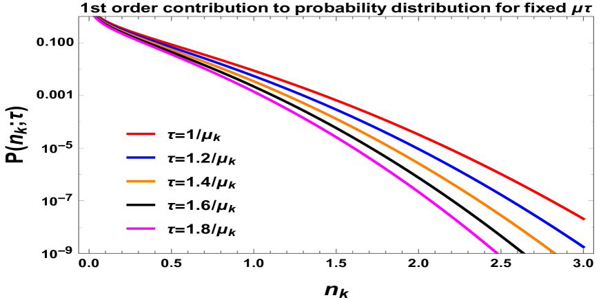
Refer to caption
Figure 38: Evolution of the first order contribution to the probability density function with respect to the the occupation number per mode nksubscript𝑛𝑘n_{k}, for a fixed time.

In figure (38), we have shown the evolution of the probability density function with respect to the occupation number per mode, for a fixed time (μkτsubscript𝜇𝑘𝜏\mu_{k}\tau=fixed). For very small values of the parameter n𝑛n we have observed from the plot that the deviation from Gaussian feature is observed.

6.3.2 Second order contribution

In this context, our objective is to find out the contributions coming from second order in the Fokker Planck equation and to solve this equation numerically 282828Including the contributions from second order we will see that the Fokker Planck equation can not solvable analytically.. To serve this purpose we equate both sides of Eq (587) after Taylor expansion and compare the coefficient of δτ2𝛿superscript𝜏2\delta\tau^{2}. Consequently, we get the following partial differential equation:

𝐒𝐞𝐜𝐨𝐧𝐝𝐨𝐫𝐝𝐞𝐫𝐅𝐨𝐤𝐤𝐞𝐫𝐏𝐥𝐚𝐧𝐜𝐤𝐄𝐪𝐮𝐚𝐭𝐢𝐨𝐧:¯¯:𝐒𝐞𝐜𝐨𝐧𝐝𝐨𝐫𝐝𝐞𝐫𝐅𝐨𝐤𝐤𝐞𝐫𝐏𝐥𝐚𝐧𝐜𝐤𝐄𝐪𝐮𝐚𝐭𝐢𝐨𝐧absent\displaystyle{\color[rgb]{0,0,1}\bf\underline{Second~{}order~{}Fokker~{}Planck~{}Equation:}}
n22(1+n)24P(n;τ)n4+2n(1+3n+2n2)3P(n;τ)n3superscript𝑛22superscript1𝑛2superscript4𝑃𝑛𝜏superscript𝑛42𝑛13𝑛2superscript𝑛2superscript3𝑃𝑛𝜏superscript𝑛3\displaystyle\frac{n^{2}}{2}\left(1+n\right)^{2}\frac{\partial^{4}P(n;\tau)}{\partial n^{4}}+2n\left(1+3n+2n^{2}\right)\frac{\partial^{3}P(n;\tau)}{\partial n^{3}}
+(1+6n+6n2)2P(n;τ)n2=1μk22P(n;τ)τ2.16𝑛6superscript𝑛2superscript2𝑃𝑛𝜏superscript𝑛21subscriptsuperscript𝜇2𝑘superscript2𝑃𝑛𝜏superscript𝜏2\displaystyle+\left(1+6n+6n^{2}\right)\frac{\partial^{2}P(n;\tau)}{\partial n^{2}}=\frac{1}{\mu^{2}_{k}}\frac{\partial^{2}P(n;\tau)}{\partial\tau^{2}}. (689)

Now to solve this partial differential equation we apply method of separation of variable, using which we can write the total solution in the following form:

P(n;τ)=P1(n)P2(τ).𝑃𝑛𝜏subscript𝑃1𝑛subscript𝑃2𝜏\displaystyle P(n;\tau)=P_{1}(n)P_{2}(\tau). (690)

Further, using the solution ansatz stated in Eq (690) we get the following sets of independent differential equations, as given by:

[n22(1+n)2d4dn4+2n(1+3n+2n2)d3dn3+(1+6n+6n2)d2dn2m22]P1(n)=0,delimited-[]superscript𝑛22superscript1𝑛2superscript𝑑4𝑑superscript𝑛42𝑛13𝑛2superscript𝑛2superscript𝑑3𝑑superscript𝑛316𝑛6superscript𝑛2superscript𝑑2𝑑superscript𝑛2subscriptsuperscript𝑚22subscript𝑃1𝑛0\displaystyle\left[\frac{n^{2}}{2}\left(1+n\right)^{2}\frac{d^{4}}{dn^{4}}+2n\left(1+3n+2n^{2}\right)\frac{d^{3}}{dn^{3}}+\left(1+6n+6n^{2}\right)\frac{d^{2}}{dn^{2}}-m^{2}_{2}\right]P_{1}(n)=0,~{}~{}~{} (691)
[d2dτ2m22μk2]P2(τ)=0.delimited-[]superscript𝑑2𝑑superscript𝜏2subscriptsuperscript𝑚22subscriptsuperscript𝜇2𝑘subscript𝑃2𝜏0\displaystyle\left[\frac{d^{2}}{d\tau^{2}}-m^{2}_{2}\mu^{2}_{k}\right]P_{2}(\tau)=0. (692)

It is important to note that, the analytical solution of P1(n)subscript𝑃1𝑛P_{1}(n) is not possible for any arbitrary values of the constant m2subscript𝑚2m_{2}, except the special case m2=0subscript𝑚20m_{2}=0. For this reason we use numerical technique to solve Eq (691). On the other hand Eq (692) is exactly solvable in the present context and the solution can be written as:

P2(τ)=[C3eτm2μk+C4eτm2μk],subscript𝑃2𝜏delimited-[]subscript𝐶3superscript𝑒𝜏subscript𝑚2subscript𝜇𝑘subscript𝐶4superscript𝑒𝜏subscript𝑚2subscript𝜇𝑘\displaystyle P_{2}(\tau)=\left[C_{3}e^{\tau m_{2}\mu_{k}}+C_{4}e^{-\tau m_{2}\mu_{k}}\right], (693)

where C3subscript𝐶3C_{3} and C4subscript𝐶4C_{4} are two arbitrary constants which can be fixed by choosing proper boundary conditions.

Now we solve Eq (691) numerically for different values of m2subscript𝑚2m_{2} along with given initial condition and also we consider the special case m2=0subscript𝑚20m_{2}=0 where we solve this equation analytically. Here it important to mention that, since arbitrary values of m2subscript𝑚2m_{2} is allowed, one can consider integer as well as non integer values at the level of solution of differential equation. However, the only physically acceptable solution restrict us to only consider the integer values of m2subscript𝑚2m_{2} because such second order corrected solution of the Fokker Planck equation is directly related to the quantum effects as we have mentioned earlier. As a result such integer values of m2subscript𝑚2m_{2} can be interpreted as the (principal) quantum number i. e.

𝐐𝐮𝐚𝐧𝐭𝐮𝐦𝐍𝐮𝐦𝐛𝐞𝐫𝐈𝐈𝐈:¯m2=0,±1,±2,,±.formulae-sequence¯:𝐐𝐮𝐚𝐧𝐭𝐮𝐦𝐍𝐮𝐦𝐛𝐞𝐫𝐈𝐈𝐈absentsubscript𝑚20plus-or-minus1plus-or-minus2plus-or-minus\displaystyle{\color[rgb]{0,0,1}\bf\underline{Quantum~{}Number~{}III:}}~{}~{}~{}~{}m_{2}=0,\pm 1,\pm 2,\cdots,\pm\infty\in\mathbb{Z}. (694)

For numerical solution we take the following assumptions:

P1(n=0.001)subscript𝑃1𝑛0.001\displaystyle P_{1}(n=0.001) =\displaystyle= 100,[dP1(n)dn]n=0.001=100,[d2P1(n)dn2]n=0.001=100,formulae-sequence100subscriptdelimited-[]𝑑subscript𝑃1𝑛𝑑𝑛𝑛0.001100subscriptdelimited-[]superscript𝑑2subscript𝑃1𝑛𝑑superscript𝑛2𝑛0.001100\displaystyle 100,~{}~{}~{}\left[\frac{dP_{1}(n)}{dn}\right]_{n=0.001}=100,~{}~{}~{}\left[\frac{d^{2}P_{1}(n)}{dn^{2}}\right]_{n=0.001}=100,
[d3P1(n)dn3]n=0.001subscriptdelimited-[]superscript𝑑3subscript𝑃1𝑛𝑑superscript𝑛3𝑛0.001\displaystyle\left[\frac{d^{3}P_{1}(n)}{dn^{3}}\right]_{n=0.001} =\displaystyle= 100.100\displaystyle 100. (695)

Here we assume that the particle production rate at low n𝑛n(= 0.0010.0010.001) has a constant value and its derivatives also have same constant value for a given m2subscript𝑚2m_{2}. Getting the numerical solution we plot (P2(n,τ)subscript𝑃2𝑛𝜏P_{2}(n,\tau) vs n𝑛n) them for some particular range of n𝑛n.

Refer to caption
(a) Second order corrected distribution for m2=0subscript𝑚20m_{2}=0
Refer to caption
(b) Second order corrected distribution for m2=1subscript𝑚21m_{2}=-1
Refer to caption
(c) Second order corrected distribution for m2=1subscript𝑚21m_{2}=1
Refer to caption
(d) Second order corrected distribution LogLog plot for m2=±2,±3subscript𝑚2plus-or-minus2plus-or-minus3m_{2}=\pm 2,\pm 3
Figure 39: Evolution of probability distribution function obtained from the second order corrected Fokker-Planck equation with the occupation number n𝑛n for different value of m2subscript𝑚2m_{2}. Here we use the initial conditions as mentioned in Eq (6.3.2).

From figure 39 we can say that for m2=±2,±3subscript𝑚2plus-or-minus2plus-or-minus3m_{2}=\pm 2,\pm 3 second order corrected probability distribution function almost overlap at lower values of the occupation number n𝑛n but deviate significantly as n𝑛n increases to large number. As a consequence, for low value of n𝑛n particle production rate is independent on m2subscript𝑚2m_{2} but as n𝑛n increases they significantly deviate. It also implies that for higher values of n𝑛n the integer m2subscript𝑚2m_{2} constrains particle production rate. For m2=±1subscript𝑚2plus-or-minus1m_{2}=\pm 1 we found that the second order corrected probability distribution function significantly deviates from log normal (Gaussian) distribution and both of them explicitly show the signature of non-Gaussianity is the second order corrected distribution function. Finally, we have shown that for m2=0subscript𝑚20m_{2}=0 the amount of deviation from log normal (Gaussian) distribution is small compared to results obtained from the other values of m2subscript𝑚2m_{2}.

Now we discuss about the analytical solution of Eq (691) for the special case when we fix m2=0subscript𝑚20m_{2}=0. In this situation one can recast the Eq (691) in to the following simplified form:

[n22(1+n)2d4dn4+2n(1+3n+2n2)d3dn3+(1+6n+6n2)d2dn2]P1(n)=0delimited-[]superscript𝑛22superscript1𝑛2superscript𝑑4𝑑superscript𝑛42𝑛13𝑛2superscript𝑛2superscript𝑑3𝑑superscript𝑛316𝑛6superscript𝑛2superscript𝑑2𝑑superscript𝑛2subscript𝑃1𝑛0\displaystyle\left[\frac{n^{2}}{2}\left(1+n\right)^{2}\frac{d^{4}}{dn^{4}}+2n\left(1+3n+2n^{2}\right)\frac{d^{3}}{dn^{3}}+\left(1+6n+6n^{2}\right)\frac{d^{2}}{dn^{2}}\right]P_{1}(n)=0 (696)

Then analytical solution of Eq (696) can be written as:

P1(n)subscript𝑃1𝑛\displaystyle P_{1}(n) =\displaystyle= C1i=02Γ(ii72+12)Γ(i12i(47+i))Γ(i+12(47+i)i+1)nii72+12(2i+7i+1)i!Γ(ii7+1)Γ(12i(47+i))Γ(1+12i(47+i))subscript𝐶1superscriptsubscript𝑖02Γ𝑖𝑖7212Γ𝑖12𝑖47𝑖Γ𝑖1247𝑖𝑖1superscript𝑛𝑖𝑖72122𝑖7𝑖1𝑖Γ𝑖𝑖71Γ12𝑖47𝑖Γ112𝑖47𝑖\displaystyle-C_{1}\sum_{i=0}^{\infty}\frac{2\Gamma\left(i-\frac{i\sqrt{7}}{2}+\frac{1}{2}\right)\Gamma\left(i-\frac{1}{2}i(\sqrt{47}+i)\right)\Gamma\left(i+\frac{1}{2}(\sqrt{47}+i)i+1\right)n^{i-\frac{i\sqrt{7}}{2}+\frac{1}{2}}}{(-2i+\sqrt{7}i+1)i!\Gamma(i-i\sqrt{7}+1)\Gamma\left(-\frac{1}{2}i(\sqrt{47}+i)\right)\Gamma\left(1+\frac{1}{2}i(\sqrt{47}+i)\right)} (697)
×2F~1(32i72,ii7212;ii72+32;n)subscript2absentsubscript~𝐹132𝑖72𝑖𝑖7212𝑖𝑖7232𝑛\displaystyle~{}~{}~{}~{}~{}~{}~{}~{}~{}~{}~{}~{}~{}~{}~{}~{}~{}~{}~{}~{}~{}~{}\times\,_{2}\tilde{F}_{1}\left(\frac{3}{2}-\frac{i\sqrt{7}}{2},i-\frac{i\sqrt{7}}{2}-\frac{1}{2};i-\frac{i\sqrt{7}}{2}+\frac{3}{2};-n\right)
+C2i=0j=0m=0Γ(c)2u+1π2b1((π2b1)Γ(b+u+1))(u1)Γ(a)Γ(b1)Γ(b2)Γ(12(b+u+1))Γ(12(b+u+2))subscript𝐶2superscriptsubscript𝑖0superscriptsubscript𝑗0superscriptsubscript𝑚0Γ𝑐superscript2𝑢1𝜋superscript2𝑏1𝜋superscript2𝑏1Γ𝑏𝑢1𝑢1Γ𝑎Γsubscript𝑏1Γsubscript𝑏2Γ12𝑏𝑢1Γ12𝑏𝑢2\displaystyle+C_{2}\sum_{i=0}^{\infty}\sum_{j=0}^{\infty}\sum_{m=0}^{\infty}\frac{\Gamma(c)2^{u+1}\sqrt{\pi}2^{-b-1}((\sqrt{\pi}2^{-b-1})\Gamma(b+u+1))}{(u-1)\Gamma(a)\Gamma(b_{1})\Gamma(b_{2})\Gamma\left(\frac{1}{2}(b+u+1)\right)\Gamma\left(\frac{1}{2}(b+u+2)\right)}
×2j(1)m+u2+1ni+m+u12+1Γ(12(b+u+1)+i)Γ(12(b+u+2)+i)i!j!m!(i+m+u12+1)Γ(b+i+32)Γ(c+j+m)absentsuperscript2𝑗superscript1𝑚𝑢21superscript𝑛𝑖𝑚𝑢121Γ12𝑏𝑢1𝑖Γ12𝑏𝑢2𝑖𝑖𝑗𝑚𝑖𝑚𝑢121Γ𝑏𝑖32Γ𝑐𝑗𝑚\displaystyle\times\frac{2^{j}(-1)^{m+\frac{u}{2}+1}n^{i+m+\frac{u-1}{2}+1}\Gamma\left(\frac{1}{2}(b+u+1)+i\right)\Gamma\left(\frac{1}{2}(b+u+2)+i\right)}{i!j!m!\left(i+m+\frac{u-1}{2}+1\right)\Gamma\left(b+i+\frac{3}{2}\right)\Gamma(c+j+m)}
×Γ(b1+m)Γ(b2+n)Γ(a+j+m).absentΓsubscript𝑏1𝑚Γsubscript𝑏2𝑛Γ𝑎𝑗𝑚\displaystyle~{}~{}~{}~{}~{}~{}~{}~{}~{}~{}~{}~{}~{}~{}~{}~{}~{}~{}~{}~{}~{}~{}~{}~{}~{}~{}~{}~{}~{}~{}~{}~{}~{}~{}~{}~{}~{}~{}~{}~{}~{}~{}~{}\times\Gamma(b_{1}+m)\Gamma(b_{2}+n)\Gamma(a+j+m).

where a𝑎a, b𝑏b, c𝑐c, b1subscript𝑏1b_{1}, b2subscript𝑏2b_{2} and u𝑢u are all functions of i𝑖i which is summed over and we have introduced them to use shorthand notation. In this context the functional dependence of all of these i𝑖i dependent parameters are given by the following expressions:

a=a(i)𝑎𝑎𝑖\displaystyle a=a(i) =\displaystyle= 12(1+i7),b=b(i)=12i(47+i),121𝑖7𝑏𝑏𝑖12𝑖47𝑖\displaystyle\frac{1}{2}\left(-1+i\sqrt{7}\right),~{}~{}~{}b=b(i)=\frac{1}{2}i\left(\sqrt{47}+i\right),
c=c(i)𝑐𝑐𝑖\displaystyle c=c(i) =\displaystyle= 12(1+i7),b1=b1(i)=12(3i7),121𝑖7subscript𝑏1subscript𝑏1𝑖123𝑖7\displaystyle\frac{1}{2}\left(1+i\sqrt{7}\right),~{}~{}~{}b_{1}=b_{1}(i)=\frac{1}{2}\left(3-i\sqrt{7}\right),
b2=b2(i)subscript𝑏2subscript𝑏2𝑖\displaystyle b_{2}=b_{2}(i) =\displaystyle= 12(4i+27i+47i+1),u=u(i)=i7.124𝑖27𝑖47𝑖1𝑢𝑢𝑖𝑖7\displaystyle\frac{1}{2}\left(4i+2\sqrt{7}i+\sqrt{47}i+1\right),~{}~{}~{}u=u(i)=i\sqrt{7}. (698)

The solution contains generalized Hypergeometric PFQ Regularized function. Also C1subscript𝐶1C_{1} and C2subscript𝐶2C_{2} are arbitrary constant of integration which can be evaluated by imposing appropriate initial conditions.

For m2=0subscript𝑚20m_{2}=0 the total probability distribution function can be expressed as:

P(n;τ)𝑃𝑛𝜏\displaystyle P(n;\tau) =\displaystyle= [C1i=02Γ(ii72+12)Γ(i12i(47+i))Γ(i+12(47+i)i+1)nii72+12(2i+7i+1)i!Γ(ii7+1)Γ(12i(47+i))Γ(1+12i(47+i))\displaystyle\left[-C_{1}\sum_{i=0}^{\infty}\frac{2\Gamma\left(i-\frac{i\sqrt{7}}{2}+\frac{1}{2}\right)\Gamma\left(i-\frac{1}{2}i(\sqrt{47}+i)\right)\Gamma\left(i+\frac{1}{2}(\sqrt{47}+i)i+1\right)n^{i-\frac{i\sqrt{7}}{2}+\frac{1}{2}}}{(-2i+\sqrt{7}i+1)i!\Gamma(i-i\sqrt{7}+1)\Gamma\left(-\frac{1}{2}i(\sqrt{47}+i)\right)\Gamma\left(1+\frac{1}{2}i(\sqrt{47}+i)\right)}\right. (699)
×2F~1(32i72,ii7212;ii72+32;n)subscript2absentsubscript~𝐹132𝑖72𝑖𝑖7212𝑖𝑖7232𝑛\displaystyle\left.~{}~{}~{}~{}~{}~{}~{}~{}~{}~{}~{}~{}~{}~{}~{}~{}~{}~{}~{}~{}~{}~{}\times\,_{2}\tilde{F}_{1}\left(\frac{3}{2}-\frac{i\sqrt{7}}{2},i-\frac{i\sqrt{7}}{2}-\frac{1}{2};i-\frac{i\sqrt{7}}{2}+\frac{3}{2};-n\right)\right.
+C2i=0j=0m=0Γ(c)2u+1π2b1((π2b1)Γ(b+u+1))(u1)Γ(a)Γ(b1)Γ(b2)Γ(12(b+u+1))Γ(12(b+u+2))subscript𝐶2superscriptsubscript𝑖0superscriptsubscript𝑗0superscriptsubscript𝑚0Γ𝑐superscript2𝑢1𝜋superscript2𝑏1𝜋superscript2𝑏1Γ𝑏𝑢1𝑢1Γ𝑎Γsubscript𝑏1Γsubscript𝑏2Γ12𝑏𝑢1Γ12𝑏𝑢2\displaystyle\left.+C_{2}\sum_{i=0}^{\infty}\sum_{j=0}^{\infty}\sum_{m=0}^{\infty}\frac{\Gamma(c)2^{u+1}\sqrt{\pi}2^{-b-1}((\sqrt{\pi}2^{-b-1})\Gamma(b+u+1))}{(u-1)\Gamma(a)\Gamma(b_{1})\Gamma(b_{2})\Gamma\left(\frac{1}{2}(b+u+1)\right)\Gamma\left(\frac{1}{2}(b+u+2)\right)}\right.
×2j(1)m+u2+1ni+m+u12+1Γ(12(b+u+1)+i)Γ(12(b+u+2)+i)i!j!m!(i+m+u12+1)Γ(b+i+32)Γ(c+j+m)absentsuperscript2𝑗superscript1𝑚𝑢21superscript𝑛𝑖𝑚𝑢121Γ12𝑏𝑢1𝑖Γ12𝑏𝑢2𝑖𝑖𝑗𝑚𝑖𝑚𝑢121Γ𝑏𝑖32Γ𝑐𝑗𝑚\displaystyle\left.\times\frac{2^{j}(-1)^{m+\frac{u}{2}+1}n^{i+m+\frac{u-1}{2}+1}\Gamma\left(\frac{1}{2}(b+u+1)+i\right)\Gamma\left(\frac{1}{2}(b+u+2)+i\right)}{i!j!m!\left(i+m+\frac{u-1}{2}+1\right)\Gamma\left(b+i+\frac{3}{2}\right)\Gamma(c+j+m)}\right.
×Γ(b1+m)Γ(b2+n)Γ(a+j+m)]\displaystyle\left.~{}~{}~{}~{}~{}~{}~{}~{}~{}~{}~{}~{}~{}~{}~{}~{}~{}~{}~{}~{}~{}~{}~{}~{}~{}~{}~{}~{}~{}~{}~{}~{}~{}~{}~{}~{}~{}~{}~{}~{}~{}~{}~{}\times\Gamma(b_{1}+m)\Gamma(b_{2}+n)\Gamma(a+j+m)\right]
×[C3eτm2μk+C4eτm2μk].absentdelimited-[]subscript𝐶3superscript𝑒𝜏subscript𝑚2subscript𝜇𝑘subscript𝐶4superscript𝑒𝜏subscript𝑚2subscript𝜇𝑘\displaystyle~{}~{}~{}~{}~{}~{}~{}~{}~{}~{}~{}~{}~{}~{}~{}~{}~{}~{}~{}~{}~{}~{}~{}~{}~{}~{}~{}~{}~{}~{}~{}~{}~{}~{}~{}~{}~{}~{}~{}~{}~{}\times\left[C_{3}e^{\tau m_{2}\mu_{k}}+C_{4}e^{-\tau m_{2}\mu_{k}}\right].

For the special case m2=0subscript𝑚20m_{2}=0 and considering the large n𝑛n limit (n𝑛n\rightarrow\infty) the Eq (696) reduces to the following form:

[n44d4dn4+2n3d3dn3+3n2d2dn2]P1(n)=0delimited-[]superscript𝑛44superscript𝑑4𝑑superscript𝑛42superscript𝑛3superscript𝑑3𝑑superscript𝑛33superscript𝑛2superscript𝑑2𝑑superscript𝑛2subscript𝑃1𝑛0\displaystyle\left[\frac{n^{4}}{4}\frac{d^{4}}{dn^{4}}+2n^{3}\frac{d^{3}}{dn^{3}}+3n^{2}\frac{d^{2}}{dn^{2}}\right]P_{1}(n)=0 (700)

After solving Eq (583) we get the following solution in the large n𝑛n limit:

P1(n)=[16(C5n2+3C6n)+C7n+C8],subscript𝑃1𝑛delimited-[]16subscript𝐶5superscript𝑛23subscript𝐶6𝑛subscript𝐶7𝑛subscript𝐶8\displaystyle P_{1}(n)=\left[\frac{1}{6}\left(\frac{C_{5}}{n^{2}}+\frac{3C_{6}}{n}\right)+C_{7}n+C_{8}\right], (701)

where C5subscript𝐶5C_{5}, C6subscript𝐶6C_{6}, C7subscript𝐶7C_{7} and C8subscript𝐶8C_{8} are the arbitrary constants of integration which can be evaluated by imposing appropriate initial condition.

In the large n𝑛n limit with m2=0subscript𝑚20m_{2}=0 the total probability distribution function can be expressed as:

P(n;τ)𝑃𝑛𝜏\displaystyle P(n;\tau) =\displaystyle= [16(C5n2+3C6n)+C7n+C8][C3eτm2μk+C4eτm2μk],delimited-[]16subscript𝐶5superscript𝑛23subscript𝐶6𝑛subscript𝐶7𝑛subscript𝐶8delimited-[]subscript𝐶3superscript𝑒𝜏subscript𝑚2subscript𝜇𝑘subscript𝐶4superscript𝑒𝜏subscript𝑚2subscript𝜇𝑘\displaystyle\left[\frac{1}{6}\left(\frac{C_{5}}{n^{2}}+\frac{3C_{6}}{n}\right)+C_{7}n+C_{8}\right]\left[C_{3}e^{\tau m_{2}\mu_{k}}+C_{4}e^{-\tau m_{2}\mu_{k}}\right], (702)

which shows huge deviation from log normal (Gaussian) distribution.

Further using the Fourier transformation with respect to the occupation number n𝑛n as mentioned in Eq (655), we get the following simplified expression for the Fokker Planck equation at the second order:

2P¯(k;τ)τ2=μk2[n22(1+n)2k42ink3(1+3n+2n2)k2(1+6n+6n2)]P¯(k;τ),superscript2¯𝑃𝑘𝜏superscript𝜏2subscriptsuperscript𝜇2𝑘delimited-[]superscript𝑛22superscript1𝑛2superscript𝑘42𝑖𝑛superscript𝑘313𝑛2superscript𝑛2superscript𝑘216𝑛6superscript𝑛2¯𝑃𝑘𝜏\displaystyle\frac{\partial^{2}\bar{P}(k;\tau)}{\partial\tau^{2}}=\mu^{2}_{k}\left[\frac{n^{2}}{2}(1+n)^{2}k^{4}-2ink^{3}(1+3n+2n^{2})-k^{2}(1+6n+6n^{2})\right]\bar{P}(k;\tau), (703)

which is obviously a simplest version of the Fokker Planck equation as it contains only two derivative with respect to time τ𝜏\tau. In the present context we get the following result for the probability distribution function in the Fourier transformed space, as given by:

P¯(k;τ|n;τ)¯𝑃𝑘conditional𝜏superscript𝑛superscript𝜏\displaystyle\bar{P}(k;\tau|n^{{}^{\prime}};\tau^{{}^{\prime}}) =\displaystyle= C1exp[𝒢(k;n)(ττ)]+C2exp[𝒢(k;n)(ττ)],subscript𝐶1𝒢𝑘superscript𝑛𝜏superscript𝜏subscript𝐶2𝒢𝑘superscript𝑛𝜏superscript𝜏\displaystyle C_{1}~{}\exp\left[{\cal G}(k;n^{{}^{\prime}})~{}(\tau-\tau^{{}^{\prime}})\right]+C_{2}~{}\exp\left[-{\cal G}(k;n^{{}^{\prime}})~{}(\tau-\tau^{{}^{\prime}})\right], (704)

where 𝒢(k;n)𝒢𝑘superscript𝑛{\cal G}(k;n^{{}^{\prime}}) is defined as:

𝒢(k;n)=μk{(n)22(1+n)2k42ink3(1+3n+2(n)2)k2(1+6n+6(n)2)}.𝒢𝑘superscript𝑛subscript𝜇𝑘superscriptsuperscript𝑛22superscript1superscript𝑛2superscript𝑘42𝑖superscript𝑛superscript𝑘313superscript𝑛2superscriptsuperscript𝑛2superscript𝑘216superscript𝑛6superscriptsuperscript𝑛2\displaystyle{\cal G}(k;n^{{}^{\prime}})=\mu_{k}\sqrt{\left\{\frac{(n^{{}^{\prime}})^{2}}{2}(1+n^{{}^{\prime}})^{2}k^{4}-2in^{{}^{\prime}}k^{3}(1+3n^{{}^{\prime}}+2(n^{{}^{\prime}})^{2})-k^{2}(1+6n^{{}^{\prime}}+6(n^{{}^{\prime}})^{2})\right\}}. (705)

Additionally, C1subscript𝐶1C_{1} and C2subscript𝐶2C_{2} are arbitrary constants which is fixed by the following two fold boundary conditions, as given by:

P(n;τ|n=0;τ=τ)\displaystyle P(n;\tau|n^{{}^{\prime}}=0;\tau^{{}^{\prime}}=\tau) =\displaystyle= δ(n),𝛿𝑛\displaystyle\delta(n), (706)
(P(n;τ|n;τ)τ)n=0,τ=τsubscript𝑃𝑛conditional𝜏superscript𝑛superscript𝜏𝜏formulae-sequencesuperscript𝑛0superscript𝜏𝜏\displaystyle\left(\frac{\partial P(n;\tau|n^{{}^{\prime}};\tau^{{}^{\prime}})}{\partial\tau}\right)_{n^{{}^{\prime}}=0,\tau^{{}^{\prime}}=\tau} =\displaystyle= δ(n)n,𝛿𝑛𝑛\displaystyle-\frac{\delta(n)}{n}, (707)

which are necessary to solve the above mentioned second order differential equation.

As a result, we get the following set of constraints equations:

C1+C2subscript𝐶1subscript𝐶2\displaystyle C_{1}+C_{2} =\displaystyle= 1,1\displaystyle 1,
C1C2subscript𝐶1subscript𝐶2\displaystyle C_{1}-C_{2} =\displaystyle= 1iμkkn,1𝑖subscript𝜇𝑘𝑘𝑛\displaystyle-\frac{1}{i\mu_{k}kn}, (708)

Solving these equations we get:

C1subscript𝐶1\displaystyle C_{1} =\displaystyle= 12(11iμkkn),1211𝑖subscript𝜇𝑘𝑘𝑛\displaystyle\frac{1}{2}\left(1-\frac{1}{i\mu_{k}kn}\right), (709)
C2subscript𝐶2\displaystyle C_{2} =\displaystyle= 12(1+1iμkkn).1211𝑖subscript𝜇𝑘𝑘𝑛\displaystyle\frac{1}{2}\left(1+\frac{1}{i\mu_{k}kn}\right). (710)

Using this solution we get the following probability distribution function in Fourier space with n=0superscript𝑛0n^{{}^{\prime}}=0 and τ=0superscript𝜏0\tau^{{}^{\prime}}=0, as given by:

P¯(k;τ)=¯𝑃𝑘𝜏absent\displaystyle\bar{P}(k;\tau)= cos(μkkτ)sin(μkkτ)μkkn.subscript𝜇𝑘𝑘𝜏subscript𝜇𝑘𝑘𝜏subscript𝜇𝑘𝑘𝑛\displaystyle\cos(\mu_{k}k\tau)-\frac{\sin(\mu_{k}k\tau)}{\mu_{k}kn}. (711)

Hence substituting back the above mentioned result into the definition of Fourier transformation and setting the initial condition n=0superscript𝑛0n^{{}^{\prime}}=0 and τ=0superscript𝜏0\tau^{{}^{\prime}}=0 we get the following result for the probability distribution function, as given by:

P(n;τ)=12π𝑑kexp[ikn](cos(μkkτ)sin(μkkτ)μkkn).𝑃𝑛𝜏12𝜋subscriptsuperscriptdifferential-d𝑘𝑖𝑘𝑛subscript𝜇𝑘𝑘𝜏subscript𝜇𝑘𝑘𝜏subscript𝜇𝑘𝑘𝑛\displaystyle P(n;\tau)=\frac{1}{2\pi}\int^{\infty}_{-\infty}dk~{}\exp[ikn]\left(\cos(\mu_{k}k\tau)-\frac{\sin(\mu_{k}k\tau)}{\mu_{k}kn}\right). (712)

However this integral is not convergent within <k<𝑘-\infty<k<\infty. For this reason we introduce a momentum cut-off ΛC<k<ΛCsubscriptΛ𝐶𝑘subscriptΛ𝐶-\Lambda_{C}<k<\Lambda_{C}. Consequently, we get the following regularised expression for the probability distribution function:

P(n;τ)𝑃𝑛𝜏\displaystyle P(n;\tau) =\displaystyle= nsin(ΛCn)cos(ΛCμkτ)μkτcos(ΛCn)sin(ΛCμkτ)π(n2μk2τ2)𝑛subscriptΛ𝐶𝑛subscriptΛ𝐶subscript𝜇𝑘𝜏subscript𝜇𝑘𝜏subscriptΛ𝐶𝑛subscriptΛ𝐶subscript𝜇𝑘𝜏𝜋superscript𝑛2subscriptsuperscript𝜇2𝑘superscript𝜏2\displaystyle\frac{n\sin(\Lambda_{C}n)\cos(\Lambda_{C}\mu_{k}\tau)-\mu_{k}\tau\cos(\Lambda_{C}n)\sin(\Lambda_{C}\mu_{k}\tau)}{\pi(n^{2}-\mu^{2}_{k}\tau^{2})} (713)
14πμkn[i(Ci(ΛC(n+μkτ))Ci(ΛC(n+μkτ))Ci(ΛCμkτnΛC)\displaystyle~{}~{}-\frac{1}{4\pi\mu_{k}n}\left[i(\text{Ci}(-\Lambda_{C}(n+\mu_{k}\tau))-\text{Ci}(\Lambda_{C}(n+\mu_{k}\tau))-\text{Ci}(\Lambda_{C}\mu_{k}\tau-n\Lambda_{C})\right.
+Ci(ΛC(nμkτ))2iSi(ΛC(n+μkτ))+2iSi(ΛC(nμkτ)))].\displaystyle\left.~{}~{}+\text{Ci}(\Lambda_{C}(n-\mu_{k}\tau))-2i\text{Si}(\Lambda_{C}(n+\mu_{k}\tau))+2i\text{Si}(\Lambda_{C}(n-\mu_{k}\tau)))\right].

which is coming from the second contribution in the Fokker Planck equation.
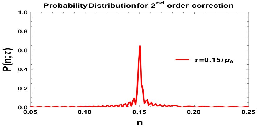
Refer to caption
Figure 40: Second order contribution to the probability density function with respect to the the occupation number per mode n𝑛n, for a fixed time from the analytical solution[713] of second order equation[6.3.2].

In figure [40], we have shown the probability density function for second order correction with respect to the occupation number per mode, for a fixed time (τ=0.15μk𝜏0.15subscript𝜇𝑘\tau=\frac{0.15}{\mu_{k}}). From this plot we have observed irregular oscillations with deviation from Gaussian feature.We have selected a high value for momentum cutoff[λcsubscript𝜆𝑐\lambda_{c}] for this particular plot.

6.3.3 Third order correction

In this context, our objective is to find out the contributions coming from third order in the Fokker Planck equation and to solve this equation numerically 292929Including the contributions from third order we will see that the Fokker Planck equation can not solvable analytically.. To serve this purpose we equate both sides of Eq (587) after Taylor expansion and compare the coefficient of δτ3𝛿superscript𝜏3\delta\tau^{3}. Consequently, we get the following partial differential equation:

n36(1+n)36P(n;τ)n6superscript𝑛36superscript1𝑛3superscript6𝑃𝑛𝜏superscript𝑛6\displaystyle\frac{n^{3}}{6}(1+n)^{3}\frac{\partial^{6}P(n;\tau)}{\partial n^{6}}
+3n22(1+n)2(1+2n)5P(n;τ)n53superscript𝑛22superscript1𝑛212𝑛superscript5𝑃𝑛𝜏superscript𝑛5\displaystyle+\frac{3n^{2}}{2}(1+n)^{2}(1+2n)\frac{\partial^{5}P(n;\tau)}{\partial n^{5}}
+3n(1+n)(1+5n+5n2)4P(n;τ)n43𝑛1𝑛15𝑛5superscript𝑛2superscript4𝑃𝑛𝜏superscript𝑛4\displaystyle+3n(1+n)(1+5n+5n^{2})\frac{\partial^{4}P(n;\tau)}{\partial n^{4}}
+(1+2n)(1+10n+10n2)3P(n;τ)n3=1μk33P(n;τ)τ312𝑛110𝑛10superscript𝑛2superscript3𝑃𝑛𝜏superscript𝑛31subscriptsuperscript𝜇3𝑘superscript3𝑃𝑛𝜏superscript𝜏3\displaystyle+(1+2n)(1+10n+10n^{2})\frac{\partial^{3}P(n;\tau)}{\partial n^{3}}=\frac{1}{\mu^{3}_{k}}\frac{\partial^{3}P(n;\tau)}{\partial\tau^{3}} (714)

which can not able to solve analytically with any integer values of m3subscript𝑚3m_{3}. We solve this equation for different values of m3subscript𝑚3m_{3} numerically with assumed initial condition. Only for the special case, m3=0subscript𝑚30m_{3}=0 with large n𝑛n limit we can able to provide an analytical solution in the present context.

Now to solve this partial differential equation we apply method of separation of variable, using which we can write the total solution in the following form:

P(n;τ)=P1(n)P2(τ).𝑃𝑛𝜏subscript𝑃1𝑛subscript𝑃2𝜏\displaystyle P(n;\tau)=P_{1}(n)P_{2}(\tau). (715)

Further, using the solution ansatz stated in Eq (690) we get the following sets of independent differential equations, as given by:

n36(1+n)3d6P1(n)dn6superscript𝑛36superscript1𝑛3superscript𝑑6subscript𝑃1𝑛𝑑superscript𝑛6\displaystyle\frac{n^{3}}{6}(1+n)^{3}\frac{d^{6}P_{1}(n)}{dn^{6}}
+3n22(1+n)2(1+2n)d5P1(n)dn53superscript𝑛22superscript1𝑛212𝑛superscript𝑑5subscript𝑃1𝑛𝑑superscript𝑛5\displaystyle+\frac{3n^{2}}{2}(1+n)^{2}(1+2n)\frac{d^{5}P_{1}(n)}{dn^{5}}
+3n(1+n)(1+5n+5n2)d4P1(n)dn43𝑛1𝑛15𝑛5superscript𝑛2superscript𝑑4subscript𝑃1𝑛𝑑superscript𝑛4\displaystyle+3n(1+n)(1+5n+5n^{2})\frac{d^{4}P_{1}(n)}{dn^{4}}
+(1+2n)(1+10n+10n2)d3P1(n)dn3m32P1(n)=0,12𝑛110𝑛10superscript𝑛2superscript𝑑3subscript𝑃1𝑛𝑑superscript𝑛3subscriptsuperscript𝑚23subscript𝑃1𝑛0\displaystyle+(1+2n)(1+10n+10n^{2})\frac{d^{3}P_{1}(n)}{dn^{3}}-m^{2}_{3}P_{1}(n)=0, (716)
[d3dτ3m32μk3]P2(τ)=0.delimited-[]superscript𝑑3𝑑superscript𝜏3subscriptsuperscript𝑚23subscriptsuperscript𝜇3𝑘subscript𝑃2𝜏0\displaystyle\left[\frac{d^{3}}{d\tau^{3}}-m^{2}_{3}\mu^{3}_{k}\right]P_{2}(\tau)=0. (717)

It is important to note that, the analytical solution of P1(n)subscript𝑃1𝑛P_{1}(n) is not possible for any arbitrary values of the constant m3subscript𝑚3m_{3}, except the special case m3=0subscript𝑚30m_{3}=0. For this reason we use numerical technique to solve Eq (716). On the other hand Eq (717) is exactly solvable in the present context and the solution can be written as:

P2(τ)=[C7e(1)2/3m32/3τμk+C8e13m32/3τμk+C9em32/3τμk],subscript𝑃2𝜏delimited-[]subscript𝐶7superscript𝑒superscript123superscriptsubscript𝑚323𝜏subscript𝜇𝑘subscript𝐶8superscript𝑒31superscriptsubscript𝑚323𝜏subscript𝜇𝑘subscript𝐶9superscript𝑒superscriptsubscript𝑚323𝜏subscript𝜇𝑘\displaystyle P_{2}(\tau)=\left[C_{7}e^{(-1)^{2/3}m_{3}^{2/3}\tau\mu_{k}}+C_{8}e^{-\sqrt[3]{-1}m_{3}^{2/3}\tau\mu_{k}}+C_{9}e^{m_{3}^{2/3}\tau\mu_{k}}\right], (718)

where C7subscript𝐶7C_{7}, C8subscript𝐶8C_{8} and C9subscript𝐶9C_{9} are three arbitrary constants which can be fixed by choosing proper boundary conditions.

Now to solve Eq (716) numerically for different values of m3subscript𝑚3m_{3} along with given initial condition and we also prove the analytical solution for the special case m3=0subscript𝑚30m_{3}=0. Here it important to mention that, since arbitrary values of m3subscript𝑚3m_{3} is allowed, one can consider integer as well as non integer values at the level of solution of differential equation. However, the only physically acceptable solution restrict us to only consider the integer values of m3subscript𝑚3m_{3} because such third order corrected solution of the Fokker Planck equation is directly related to the quantum effects as we have mentioned earlier. As a result such integer values of m3subscript𝑚3m_{3} can be interpreted as the quantum number i. e.

𝐐𝐮𝐚𝐧𝐭𝐮𝐦𝐍𝐮𝐦𝐛𝐞𝐫𝐈𝐕:¯m3=0,±1,±2,,±.formulae-sequence¯:𝐐𝐮𝐚𝐧𝐭𝐮𝐦𝐍𝐮𝐦𝐛𝐞𝐫𝐈𝐕absentsubscript𝑚30plus-or-minus1plus-or-minus2plus-or-minus\displaystyle{\color[rgb]{0,0,1}\bf\underline{Quantum~{}Number~{}IV:}}~{}~{}~{}~{}m_{3}=0,\pm 1,\pm 2,\cdots,\pm\infty\in\mathbb{Z}. (719)

For numerical solution we take the following assumptions:

P1(n=0.0001)subscript𝑃1𝑛0.0001\displaystyle P_{1}(n=0.0001) =\displaystyle= 100,[dP1(n)dn]n=0.0001=100,100subscriptdelimited-[]𝑑subscript𝑃1𝑛𝑑𝑛𝑛0.0001100\displaystyle 100,~{}~{}~{}~{}~{}~{}\left[\frac{dP_{1}(n)}{dn}\right]_{n=0.0001}=100,
[d2P1(n)dn2]n=0.0001subscriptdelimited-[]superscript𝑑2subscript𝑃1𝑛𝑑superscript𝑛2𝑛0.0001\displaystyle\left[\frac{d^{2}P_{1}(n)}{dn^{2}}\right]_{n=0.0001} =\displaystyle= 100,[d3P1(n)dn3]n=0.0001]=100,\displaystyle 100,~{}~{}~{}~{}~{}~{}\left[\frac{d^{3}P_{1}(n)}{dn^{3}}\right]_{n=0.0001}]=100,
[d4P1(n)dn4]n=0.0001subscriptdelimited-[]superscript𝑑4subscript𝑃1𝑛𝑑superscript𝑛4𝑛0.0001\displaystyle\left[\frac{d^{4}P_{1}(n)}{dn^{4}}\right]_{n=0.0001} =\displaystyle= 100,[d5P1(n)dn5]n=0.0001=100.100subscriptdelimited-[]superscript𝑑5subscript𝑃1𝑛𝑑superscript𝑛5𝑛0.0001100\displaystyle 100,~{}~{}~{}~{}~{}~{}\left[\frac{d^{5}P_{1}(n)}{dn^{5}}\right]_{n=0.0001}=100. (720)

Asper our assumption particle production probability has constant value at some particular small n[0.00010.00010.0001] or for small n P[n,τ]𝑃𝑛𝜏P[n,\tau] and all its derivative has constant values and all those values are same.

Refer to caption
(a) Third order corrected distribution for m3=0,1,2,3subscript𝑚30123m_{3}=0,1,2,3
Refer to caption
(b) Third order corrected distribution for m3=0,1,2,3subscript𝑚30123m_{3}=0,-1,-2,-3
Figure 41: Evolution of probability distribution function obtained from the third order corrected Fokker-Planck equation with the occupation number n𝑛n for different value of m3subscript𝑚3m_{3}. Here we use the initial conditions as mentioned in Eq (6.3.3).

From Fig 41 one can say that the third order corrected probability distribution function for different value of m3=0subscript𝑚30m_{3}=0 overlap at lower n𝑛n limit (n 0absent0\rightarrow 0) though deviate significantly at large n𝑛n limit. At lower values of n𝑛n, particle production probability is independent of m3subscript𝑚3m_{3} and almost flat. But as soon as n𝑛n reaches values greater than unity the distribution increase exponentially and for different m3subscript𝑚3m_{3} they differ from each other.

Now we discuss about the analytical solution of Eq (716) for the special case when we fix m3=0subscript𝑚30m_{3}=0. In this situation one can recast the Eq (716) in to the following simplified form:

n36(1+n)3d6P1(n)dn6superscript𝑛36superscript1𝑛3superscript𝑑6subscript𝑃1𝑛𝑑superscript𝑛6\displaystyle\frac{n^{3}}{6}(1+n)^{3}\frac{d^{6}P_{1}(n)}{dn^{6}}
+3n22(1+n)2(1+2n)d5P1(n)dn53superscript𝑛22superscript1𝑛212𝑛superscript𝑑5subscript𝑃1𝑛𝑑superscript𝑛5\displaystyle+\frac{3n^{2}}{2}(1+n)^{2}(1+2n)\frac{d^{5}P_{1}(n)}{dn^{5}}
+3n(1+n)(1+5n+5n2)d4P1(n)dn43𝑛1𝑛15𝑛5superscript𝑛2superscript𝑑4subscript𝑃1𝑛𝑑superscript𝑛4\displaystyle+3n(1+n)(1+5n+5n^{2})\frac{d^{4}P_{1}(n)}{dn^{4}}
+(1+2n)(1+10n+10n2)d3P1(n)dn3=0.12𝑛110𝑛10superscript𝑛2superscript𝑑3subscript𝑃1𝑛𝑑superscript𝑛30\displaystyle+(1+2n)(1+10n+10n^{2})\frac{d^{3}P_{1}(n)}{dn^{3}}=0. (721)

To find the analytical solution of Eq (721) one can further use the following simplification:

n3(1+n)36d3Q1(n)dn3superscript𝑛3superscript1𝑛36superscript𝑑3subscript𝑄1𝑛𝑑superscript𝑛3\displaystyle\frac{n^{3}(1+n)^{3}}{6}\frac{d^{3}Q_{1}(n)}{dn^{3}}
+3n2(1+n)2(1+2n)2d2Q1(n)dn23superscript𝑛2superscript1𝑛212𝑛2superscript𝑑2subscript𝑄1𝑛𝑑superscript𝑛2\displaystyle+\frac{3n^{2}(1+n)^{2}(1+2n)}{2}\frac{d^{2}Q_{1}(n)}{dn^{2}}
+3n(1+n)(1+5n+5n2)dQ1(n)dn3𝑛1𝑛15𝑛5superscript𝑛2𝑑subscript𝑄1𝑛𝑑𝑛\displaystyle+3n(1+n)(1+5n+5n^{2})\frac{dQ_{1}(n)}{dn}
+(1+2n)(1+10n+10n2)Q1(n)=012𝑛110𝑛10superscript𝑛2subscript𝑄1𝑛0\displaystyle+(1+2n)(1+10n+10n^{2})Q_{1}(n)=0 (722)

where we introduce a new function Q1(n)subscript𝑄1𝑛Q_{1}(n) which can be expressed in terms of P1(n)subscript𝑃1𝑛P_{1}(n) by following identification:

Q1(n)=d3P1(n)dn3.subscript𝑄1𝑛superscript𝑑3subscript𝑃1𝑛𝑑superscript𝑛3\displaystyle Q_{1}(n)=\frac{d^{3}P_{1}(n)}{dn^{3}}. (723)

On large n𝑛n limit (n𝑛n\rightarrow\infty) the Eq 6.3.3 reduces to following extremely simplified form:

n66d3Q1(n)dn3+3n5d2Q1(n)dn2+15n4dQ1(n)dn+20n3Q1(n)=0.superscript𝑛66superscript𝑑3subscript𝑄1𝑛𝑑superscript𝑛33superscript𝑛5superscript𝑑2subscript𝑄1𝑛𝑑superscript𝑛215superscript𝑛4𝑑subscript𝑄1𝑛𝑑𝑛20superscript𝑛3subscript𝑄1𝑛0\displaystyle\frac{n^{6}}{6}\frac{d^{3}Q_{1}(n)}{dn^{3}}+3n^{5}\frac{d^{2}Q_{1}(n)}{dn^{2}}+15n^{4}\frac{dQ_{1}(n)}{dn}+20n^{3}Q_{1}(n)=0. (724)

The solution of this equation at large n𝑛n limit can be expressed as:

Q1(n)subscript𝑄1𝑛\displaystyle Q_{1}(n) =\displaystyle= [C31148n15/2{(15C171C2)sin(1271lnn)\displaystyle\left[C_{3}-\frac{1}{148n^{15/2}}\left\{\left(15C_{1}-\sqrt{71}C_{2}\right)\sin\left(\frac{1}{2}\sqrt{71}\ln n\right)\right.\right. (725)
+(15C2+71C1)cos(1271lnn)+240n15/2lnn}],\displaystyle\left.\left.~{}~{}~{}~{}~{}~{}~{}~{}~{}~{}~{}~{}~{}+\left(15C_{2}+\sqrt{71}C_{1}\right)\cos\left(\frac{1}{2}\sqrt{71}\ln n\right)+240n^{15/2}\ln n\right\}\right],~{}~{}~{}

where C1subscript𝐶1C_{1},C2subscript𝐶2C_{2} and C3subscript𝐶3C_{3} are arbitrary constant of integration and can be evaluated by imposing appropriate initial condition.

Here, in the large n𝑛n limit the solution for P1(n)subscript𝑃1𝑛P_{1}(n) can be written as:

P1(n)subscript𝑃1𝑛\displaystyle P_{1}(n) =\displaystyle= [1674880n9/2{3040n15/2(37C360lnn+110)\displaystyle\left[\frac{1}{674880n^{9/2}}\left\{3040n^{15/2}\left(37C_{3}-60\ln n+110\right)\right.\right. (726)
(189C1+1771C2)sin(1271lnn)189subscript𝐶11771subscript𝐶21271𝑛\displaystyle\left.\left.~{}~{}~{}~{}~{}~{}~{}~{}~{}~{}~{}~{}~{}~{}~{}~{}~{}~{}~{}~{}~{}-\left(189C_{1}+17\sqrt{71}C_{2}\right)\sin\left(\frac{1}{2}\sqrt{71}\ln n\right)\right.\right.
+(1771C1189C2)cos(1271lnn)}\displaystyle\left.\left.~{}~{}~{}~{}~{}~{}~{}~{}~{}~{}~{}~{}~{}~{}~{}~{}~{}~{}~{}~{}~{}+\left(17\sqrt{71}C_{1}-189C_{2}\right)\cos\left(\frac{1}{2}\sqrt{71}\ln n\right)\right\}\right.
+C6n2+C5n+C4],\displaystyle\left.~{}~{}~{}~{}~{}~{}~{}~{}~{}~{}~{}~{}~{}~{}~{}~{}~{}~{}~{}~{}~{}~{}~{}~{}~{}~{}~{}~{}~{}~{}~{}~{}~{}~{}~{}~{}~{}~{}~{}~{}~{}~{}~{}~{}~{}~{}~{}~{}~{}~{}~{}~{}+C_{6}n^{2}+C_{5}n+C_{4}\right],

where C4subscript𝐶4C_{4}, C5subscript𝐶5C_{5} and C6subscript𝐶6C_{6} are arbitrary constant of integration and can be evaluated by imposing appropriate initial condition.

Finally, in the large n𝑛n limit the total probability distribution function can be expressed as:

P(n;τ)𝑃𝑛𝜏\displaystyle P(n;\tau) =\displaystyle= [1674880n9/2{3040n15/2(37C360lnn+110)\displaystyle\left[\frac{1}{674880n^{9/2}}\left\{3040n^{15/2}\left(37C_{3}-60\ln n+110\right)\right.\right. (727)
(189C1+1771C2)sin(1271lnn)189subscript𝐶11771subscript𝐶21271𝑛\displaystyle\left.\left.~{}~{}~{}~{}~{}~{}~{}~{}~{}~{}~{}~{}~{}~{}~{}~{}~{}~{}~{}~{}~{}-\left(189C_{1}+17\sqrt{71}C_{2}\right)\sin\left(\frac{1}{2}\sqrt{71}\ln n\right)\right.\right.
+(1771C1189C2)cos(1271lnn)}\displaystyle\left.\left.~{}~{}~{}~{}~{}~{}~{}~{}~{}~{}~{}~{}~{}~{}~{}~{}~{}~{}~{}~{}~{}+\left(17\sqrt{71}C_{1}-189C_{2}\right)\cos\left(\frac{1}{2}\sqrt{71}\ln n\right)\right\}\right.
+C6n2+C5n+C4]\displaystyle\left.~{}~{}~{}~{}~{}~{}~{}~{}~{}~{}~{}~{}~{}~{}~{}~{}~{}~{}~{}~{}~{}~{}~{}~{}~{}~{}~{}~{}~{}~{}~{}~{}~{}~{}~{}~{}~{}~{}~{}~{}~{}~{}~{}~{}~{}~{}~{}~{}~{}~{}~{}~{}+C_{6}n^{2}+C_{5}n+C_{4}\right]
×[C7e(1)2/3m32/3τμk+C8e13m32/3τμk+C9em32/3τμk],absentdelimited-[]subscript𝐶7superscript𝑒superscript123superscriptsubscript𝑚323𝜏subscript𝜇𝑘subscript𝐶8superscript𝑒31superscriptsubscript𝑚323𝜏subscript𝜇𝑘subscript𝐶9superscript𝑒superscriptsubscript𝑚323𝜏subscript𝜇𝑘\displaystyle\times\left[C_{7}e^{(-1)^{2/3}m_{3}^{2/3}\tau\mu_{k}}+C_{8}e^{-\sqrt[3]{-1}m_{3}^{2/3}\tau\mu_{k}}+C_{9}e^{m_{3}^{2/3}\tau\mu_{k}}\right],

which shows large deviation from log normal (Gaussian) distribution.

Further using the Fourier transformation with respect to the occupation number n𝑛n as mentioned in Eq (655), we get the following simplified expression for the Fokker Planck equation at the third order:

3P¯(k;τ)τ3superscript3¯𝑃𝑘𝜏superscript𝜏3\displaystyle\frac{\partial^{3}\bar{P}(k;\tau)}{\partial\tau^{3}} =\displaystyle= μk3[n36(1+n)3k6+3n2i2(1+n)2(1+2n)k5\displaystyle\mu^{3}_{k}\left[-\frac{n^{3}}{6}(1+n)^{3}k^{6}+\frac{3n^{2}i}{2}(1+n)^{2}(1+2n)k^{5}\right. (728)
+3n(1+n)(1+5n+5n2)k4ik3(1+2n)(1+10n+10n2)]P¯(k;τ),\displaystyle\left.+3n(1+n)(1+5n+5n^{2})k^{4}-ik^{3}(1+2n)(1+10n+10n^{2})\right]\bar{P}(k;\tau),~{}~{}~{}~{}~{}~{}~{}~{}~{}~{}

which is obviously a simplest version of the Fokker Planck equation as it contains only three derivative with respect to time τ𝜏\tau. In the present context we get the following result for the probability distribution function in the Fourier transformed space, as given by:

P¯(k;τ|n;τ)¯𝑃𝑘conditional𝜏superscript𝑛superscript𝜏\displaystyle\bar{P}(k;\tau|n^{{}^{\prime}};\tau^{{}^{\prime}}) =\displaystyle= C1exp[(1)2/3𝒪(k;n)3(ττ)]subscript𝐶1superscript1233𝒪𝑘superscript𝑛𝜏superscript𝜏\displaystyle C_{1}~{}\exp\left[(-1)^{2/3}\sqrt[3]{{\cal O}(k;n^{{}^{\prime}})}~{}(\tau-\tau^{{}^{\prime}})\right] (729)
+C2exp[(1)1/3𝒪(k;n)3(ττ)]subscript𝐶2superscript1133𝒪𝑘superscript𝑛𝜏superscript𝜏\displaystyle~{}~{}~{}+C_{2}~{}\exp\left[(-1)^{1/3}\sqrt[3]{{\cal O}(k;n^{{}^{\prime}})}~{}(\tau-\tau^{{}^{\prime}})\right]
+C3exp[𝒪(k;n)3(ττ)],subscript𝐶33𝒪𝑘superscript𝑛𝜏superscript𝜏\displaystyle~{}~{}~{}~{}~{}~{}~{}~{}~{}~{}+C_{3}~{}\exp\left[\sqrt[3]{{\cal O}(k;n^{{}^{\prime}})}~{}(\tau-\tau^{{}^{\prime}})\right],

where 𝒪(k;n)𝒪𝑘superscript𝑛{\cal O}(k;n^{{}^{\prime}}) is defined as:

𝒪(k;n)𝒪𝑘superscript𝑛\displaystyle{\cal O}(k;n^{{}^{\prime}}) =\displaystyle= μk3[(n)36(1+n)3k6+3(n)2i2(1+n)2(1+2n)k5\displaystyle\mu^{3}_{k}\left[-\frac{(n^{{}^{\prime}})^{3}}{6}(1+n^{{}^{\prime}})^{3}k^{6}+\frac{3(n^{{}^{\prime}})^{2}i}{2}(1+n^{{}^{\prime}})^{2}(1+2n^{{}^{\prime}})k^{5}\right. (730)
+3n(1+n)(1+5n+5(n)2)k4ik3(1+2n)(1+10n+10(n)2)].\displaystyle\left.+3n^{{}^{\prime}}(1+n^{{}^{\prime}})(1+5n^{{}^{\prime}}+5(n^{{}^{\prime}})^{2})k^{4}-ik^{3}(1+2n^{{}^{\prime}})(1+10n^{{}^{\prime}}+10(n^{{}^{\prime}})^{2})\right].~{}~{}~{}~{}~{}~{}

Additionally, C1subscript𝐶1C_{1} , C2subscript𝐶2C_{2} and C3subscript𝐶3C_{3} are arbitrary constants which is fixed by the following three fold boundary conditions, as given by:

P(n;τ|n=0;τ=τ)\displaystyle P(n;\tau|n^{{}^{\prime}}=0;\tau^{{}^{\prime}}=\tau) =\displaystyle= δ(n),𝛿𝑛\displaystyle\delta(n), (731)
(P(n;τ|n;τ)τ)n=0,τ=τsubscript𝑃𝑛conditional𝜏superscript𝑛superscript𝜏𝜏formulae-sequencesuperscript𝑛0𝜏superscript𝜏\displaystyle\left(\frac{\partial P(n;\tau|n^{{}^{\prime}};\tau^{{}^{\prime}})}{\partial\tau}\right)_{n^{{}^{\prime}}=0,\tau=\tau^{{}^{\prime}}} =\displaystyle= δ(n)n,𝛿𝑛𝑛\displaystyle-\frac{\delta(n)}{n}, (732)
(2P(n;τ|n;τ)τ2)n=0,τ=τsubscriptsuperscript2𝑃𝑛conditional𝜏superscript𝑛superscript𝜏superscript𝜏2formulae-sequencesuperscript𝑛0𝜏superscript𝜏\displaystyle\left(\frac{\partial^{2}P(n;\tau|n^{{}^{\prime}};\tau^{{}^{\prime}})}{\partial\tau^{2}}\right)_{n^{{}^{\prime}}=0,\tau=\tau^{{}^{\prime}}} =\displaystyle= 2δ(n)n2.2𝛿𝑛superscript𝑛2\displaystyle\frac{2~{}\delta(n)}{n^{2}}. (733)

which are necessary to solve the above mentioned third order differential equation.

As a result, we get the following set of constraints equations:

C1+C2+C3=1,subscript𝐶1subscript𝐶2subscript𝐶31\displaystyle C_{1}+C_{2}+C_{3}=1, (734)
C1(1)2/3C2(1)1/3C3=1i1/3μkkn,subscript𝐶1superscript123subscript𝐶2superscript113subscript𝐶31superscript𝑖13subscript𝜇𝑘𝑘𝑛\displaystyle C_{1}-(-1)^{2/3}~{}C_{2}-(-1)^{1/3}~{}C_{3}=\frac{1}{i^{1/3}\mu_{k}kn},~{}~{}~{}~{} (735)
C1(1)4/3C2(1)2/3C3=2i2/3μk2k2n2,subscript𝐶1superscript143subscript𝐶2superscript123subscript𝐶32superscript𝑖23subscriptsuperscript𝜇2𝑘superscript𝑘2superscript𝑛2\displaystyle C_{1}-(-1)^{4/3}C_{2}-(-1)^{2/3}C_{3}=-\frac{2}{i^{2/3}\mu^{2}_{k}k^{2}n^{2}},~{}~{}~{}~{} (736)

Solving these equations we get:

C1subscript𝐶1\displaystyle C_{1} =\displaystyle= (1)2/3(16knμkiknμk+2132)(3131)k2n2μk2,superscript12361𝑘𝑛subscript𝜇𝑘𝑖𝑘𝑛subscript𝜇𝑘23123311superscript𝑘2superscript𝑛2superscriptsubscript𝜇𝑘2\displaystyle\frac{(-1)^{2/3}\left(-\sqrt[6]{-1}kn\mu_{k}-ikn\mu_{k}+2\sqrt[3]{-1}-2\right)}{\left(3\sqrt[3]{-1}-1\right)k^{2}n^{2}\mu_{k}^{2}}, (737)
C2subscript𝐶2\displaystyle C_{2} =\displaystyle= 13(knμk(1)2/3knμk4i+216+6(1)5/6)(16i)(3131)k2n2μk2,31𝑘𝑛subscript𝜇𝑘superscript123𝑘𝑛subscript𝜇𝑘4𝑖2616superscript15661𝑖3311superscript𝑘2superscript𝑛2superscriptsubscript𝜇𝑘2\displaystyle-\frac{\sqrt[3]{-1}\left(-kn\mu_{k}-(-1)^{2/3}kn\mu_{k}-4i+2\sqrt[6]{-1}+6(-1)^{5/6}\right)}{\left(\sqrt[6]{-1}-i\right)\left(3\sqrt[3]{-1}-1\right)k^{2}n^{2}\mu_{k}^{2}}, (738)
C3subscript𝐶3\displaystyle C_{3} =\displaystyle= 13knμk(1)2/3knμk8i+1016+10(1)5/6(16i)(3131)k2n2μk2.31𝑘𝑛subscript𝜇𝑘superscript123𝑘𝑛subscript𝜇𝑘8𝑖106110superscript15661𝑖3311superscript𝑘2superscript𝑛2superscriptsubscript𝜇𝑘2\displaystyle-\frac{\sqrt[3]{-1}kn\mu_{k}-(-1)^{2/3}kn\mu_{k}-8i+10\sqrt[6]{-1}+10(-1)^{5/6}}{\left(\sqrt[6]{-1}-i\right)\left(3\sqrt[3]{-1}-1\right)k^{2}n^{2}\mu_{k}^{2}}. (739)

Using this solution get the following probability distribution function in Fourier space, as given by:

P¯(k;τ)¯𝑃𝑘𝜏\displaystyle\bar{P}(k;\tau) =\displaystyle= (1)2/3(16knμkiknμk+2132)(3131)k2n2μk2exp[i1/3μkkτ]superscript12361𝑘𝑛subscript𝜇𝑘𝑖𝑘𝑛subscript𝜇𝑘23123311superscript𝑘2superscript𝑛2superscriptsubscript𝜇𝑘2superscript𝑖13subscript𝜇𝑘𝑘𝜏\displaystyle\frac{(-1)^{2/3}\left(-\sqrt[6]{-1}kn\mu_{k}-ikn\mu_{k}+2\sqrt[3]{-1}-2\right)}{\left(3\sqrt[3]{-1}-1\right)k^{2}n^{2}\mu_{k}^{2}}~{}\exp\left[-i^{1/3}\mu_{k}k~{}\tau\right]
13(knμk(1)2/3knμk4i+216+6(1)5/6)(16i)(3131)k2n2μk2exp[(1)2/3i1/3μkkτ]31𝑘𝑛subscript𝜇𝑘superscript123𝑘𝑛subscript𝜇𝑘4𝑖2616superscript15661𝑖3311superscript𝑘2superscript𝑛2superscriptsubscript𝜇𝑘2superscript123superscript𝑖13subscript𝜇𝑘𝑘𝜏\displaystyle-\frac{\sqrt[3]{-1}\left(-kn\mu_{k}-(-1)^{2/3}kn\mu_{k}-4i+2\sqrt[6]{-1}+6(-1)^{5/6}\right)}{\left(\sqrt[6]{-1}-i\right)\left(3\sqrt[3]{-1}-1\right)k^{2}n^{2}\mu_{k}^{2}}~{}\exp\left[(-1)^{2/3}i^{1/3}\mu_{k}k~{}\tau\right]
+13knμk(1)2/3knμk8i+1016+10(1)5/6(16i)(3131)k2n2μk2exp[(1)1/3i1/3μkkτ].\displaystyle+-\frac{\sqrt[3]{-1}kn\mu_{k}-(-1)^{2/3}kn\mu_{k}-8i+10\sqrt[6]{-1}+10(-1)^{5/6}}{\left(\sqrt[6]{-1}-i\right)\left(3\sqrt[3]{-1}-1\right)k^{2}n^{2}\mu_{k}^{2}}~{}\exp\left[(-1)^{1/3}i^{1/3}\mu_{k}k~{}\tau\right].

Hence substituting back into the definition of Fourier transformation and setting the initial condition n=0superscript𝑛0n^{{}^{\prime}}=0 and τ=0superscript𝜏0\tau^{{}^{\prime}}=0 we get the following result for the probability distribution function, as given by:

P(n;τ)𝑃𝑛𝜏\displaystyle P(n;\tau) =\displaystyle= ((3+3i)μk+2(3+i))n34(3+2i)μk2n2((1)2/3μkτ+n)((1)2/3μkτ+n)233𝑖subscript𝜇𝑘23𝑖superscript𝑛3432𝑖subscriptsuperscript𝜇2𝑘superscript𝑛2superscript123subscript𝜇𝑘𝜏𝑛superscriptsuperscript123subscript𝜇𝑘𝜏𝑛2\displaystyle\frac{\left(\left(\sqrt{3}+3i\right)\mu_{k}+2\left(\sqrt{3}+i\right)\right)n^{3}}{4\left(\sqrt{3}+2i\right)\mu^{2}_{k}n^{2}\left((-1)^{2/3}\mu_{k}\tau+n\right)\sqrt{\left((-1)^{2/3}\mu_{k}\tau+n\right)^{2}}}
+2in2(2i3μk2τ+μk(13μk2τ2+n2+2(1)2/3μknτ+3i3τ+3τ)\displaystyle+2in^{2}\left(2i\sqrt{3}\mu^{2}_{k}\tau+\mu_{k}\left(\sqrt{-\sqrt[3]{-1}\mu^{2}_{k}\tau^{2}+n^{2}+2(-1)^{2/3}\mu_{k}n\tau}+3i\sqrt{3}\tau+3\tau\right)\right.
213μk2τ2+n2+2(1)2/3μknτ)μknτ(((33i))μk2τ\displaystyle\left.~{}~{}-2\sqrt{-\sqrt[3]{-1}\mu^{2}_{k}\tau^{2}+n^{2}+2(-1)^{2/3}\mu_{k}n\tau}\right)-\mu_{k}n\tau\left(\left(-\left(\sqrt{3}-3i\right)\right)\mu^{2}_{k}\tau\right.
+216μ(13μk2τ2+n2+2(1)2/3μknτ+3i3τ+3τ)261𝜇31subscriptsuperscript𝜇2𝑘superscript𝜏2superscript𝑛22superscript123subscript𝜇𝑘𝑛𝜏3𝑖3𝜏3𝜏\displaystyle\left.~{}~{}~{}~{}~{}~{}~{}~{}~{}~{}~{}~{}~{}~{}~{}+2\sqrt[6]{-1}\mu\left(\sqrt{-\sqrt[3]{-1}\mu^{2}_{k}\tau^{2}+n^{2}+2(-1)^{2/3}\mu_{k}n\tau}+3i\sqrt{3}\tau+3\tau\right)\right.
2(3i)13μk2τ2+n2+2(1)2/3μknτ)\displaystyle\left.~{}~{}~{}~{}~{}~{}~{}~{}~{}~{}~{}~{}~{}~{}~{}-2\left(\sqrt{3}-i\right)\sqrt{-\sqrt[3]{-1}\mu^{2}_{k}\tau^{2}+n^{2}+2(-1)^{2/3}\mu_{k}n\tau}\right)
+(3+i)μk2τ2(2μkτ+2i(3i)μk2τ2+4n2+4i(3+i)μknτ),3𝑖subscriptsuperscript𝜇2𝑘superscript𝜏22subscript𝜇𝑘𝜏2𝑖3𝑖subscriptsuperscript𝜇2𝑘superscript𝜏24superscript𝑛24𝑖3𝑖subscript𝜇𝑘𝑛𝜏\displaystyle~{}~{}+\left(\sqrt{3}+i\right)\mu^{2}_{k}\tau^{2}\left(2\mu_{k}\tau+\sqrt{-2i\left(\sqrt{3}-i\right)\mu^{2}_{k}\tau^{2}+4n^{2}+4i\left(\sqrt{3}+i\right)\mu_{k}n\tau}\right),

which is coming from the third contribution in the Fokker Planck equation.

Refer to caption
Figure 42: Third order contribution to the probability density function with respect to the the occupation number per mode n𝑛n, for a fixed time from the analytical solution[Eq:-LABEL:ana_3] of third order correction equation[Eq:-716]

In Fig:-42, we have shown the third order correction of probability density function with respect to the occupation number per mode, for a fixed time (μkτsubscript𝜇𝑘𝜏\mu_{k}\tau=fixed). From this plot we have observed primary gaussian feature followed by an exponential type increase.We consider the perturbative expansion to be valid. So the higher order correction contribute less than the previous order.To normalize the analytical solution we have used this. In latter part we can see the exponential type increase contribute in longer tail effect [ higher kurtosis].

6.3.4 Fourth order correction

In this context, our objective is to find out the contributions coming from fourth order in the Fokker Planck equation and to solve this equation numerically 303030Including the contributions from fourth order we will see that the Fokker Planck equation can not solvable analytically.. To serve this purpose we equate both sides of Eq (587) after Taylor expansion and compare the coefficient of δτ4𝛿superscript𝜏4\delta\tau^{4}. Consequently, we get the following partial differential equation:

70n4(1+n)48P(n;τ)n8+140n3(1+2n)7P(n;τ)n770superscript𝑛4superscript1𝑛4superscript8𝑃𝑛𝜏superscript𝑛8140superscript𝑛312𝑛superscript7𝑃𝑛𝜏superscript𝑛7\displaystyle 70n^{4}(1+n)^{4}\frac{\partial^{8}P(n;\tau)}{\partial n^{8}}+140n^{3}(1+2n)\frac{\partial^{7}P(n;\tau)}{\partial n^{7}}
+30n2(1+n)2(3+14n+14n2)6P(n;τ)n630superscript𝑛2superscript1𝑛2314𝑛14superscript𝑛2superscript6𝑃𝑛𝜏superscript𝑛6\displaystyle+30n^{2}(1+n)^{2}(3+14n+14n^{2})\frac{\partial^{6}P(n;\tau)}{\partial n^{6}}
+20n(1+n)(1+2n)(1+7n+7n2)5P(n;τ)n520𝑛1𝑛12𝑛17𝑛7superscript𝑛2superscript5𝑃𝑛𝜏superscript𝑛5\displaystyle+20n(1+n)(1+2n)(1+7n+7n^{2})\frac{\partial^{5}P(n;\tau)}{\partial n^{5}}
+(1+20n+90n2+140n3+70n4)4P(n;τ)n4=1μk44P(n;τ)τ4.120𝑛90superscript𝑛2140superscript𝑛370superscript𝑛4superscript4𝑃𝑛𝜏superscript𝑛41subscriptsuperscript𝜇4𝑘superscript4𝑃𝑛𝜏superscript𝜏4\displaystyle+(1+20n+90n^{2}+140n^{3}+70n^{4})\frac{\partial^{4}P(n;\tau)}{\partial n^{4}}=\frac{1}{\mu^{4}_{k}}\frac{\partial^{4}P(n;\tau)}{\partial\tau^{4}}. (742)

which can not able to solve analytically with any integer values of m4subscript𝑚4m_{4}. We solve this equation for different values of m4subscript𝑚4m_{4} numerically with assumed initial condition. Only for the special case, m4=0subscript𝑚40m_{4}=0 with large n𝑛n limit we can able to provide an analytical solution in the present context.

Now to solve this partial differential equation we apply method of separation of variable, using which we can write the total solution in the following form:

P(n;τ)=P1(n)P2(τ).𝑃𝑛𝜏subscript𝑃1𝑛subscript𝑃2𝜏\displaystyle P(n;\tau)=P_{1}(n)P_{2}(\tau). (743)

Further, using the solution ansatz stated in Eq (6.3.4) we get the following sets of independent differential equations, as given by:

70n4(1+n)4d8P1(n)dn8+140n3(1+2n)d7P1(n)dn770superscript𝑛4superscript1𝑛4superscript𝑑8subscript𝑃1𝑛𝑑superscript𝑛8140superscript𝑛312𝑛superscript𝑑7subscript𝑃1𝑛𝑑superscript𝑛7\displaystyle 70n^{4}(1+n)^{4}\frac{d^{8}P_{1}(n)}{dn^{8}}+140n^{3}(1+2n)\frac{d^{7}P_{1}(n)}{dn^{7}}
+30n2(1+n)2(3+14n+14n2)d6P1(n)dn630superscript𝑛2superscript1𝑛2314𝑛14superscript𝑛2superscript𝑑6subscript𝑃1𝑛𝑑superscript𝑛6\displaystyle+30n^{2}(1+n)^{2}(3+14n+14n^{2})\frac{d^{6}P_{1}(n)}{dn^{6}}
+20n(1+n)(1+2n)(1+7n+7n2)d5P1(n)dn520𝑛1𝑛12𝑛17𝑛7superscript𝑛2superscript𝑑5subscript𝑃1𝑛𝑑superscript𝑛5\displaystyle+20n(1+n)(1+2n)(1+7n+7n^{2})\frac{d^{5}P_{1}(n)}{dn^{5}}
+(1+20n+90n2+140n3+70n4)d4P1(n)dn4m42P1(n)=0,120𝑛90superscript𝑛2140superscript𝑛370superscript𝑛4superscript𝑑4subscript𝑃1𝑛𝑑superscript𝑛4subscriptsuperscript𝑚24subscript𝑃1𝑛0\displaystyle+(1+20n+90n^{2}+140n^{3}+70n^{4})\frac{d^{4}P_{1}(n)}{dn^{4}}-m^{2}_{4}P_{1}(n)=0, (744)
[d4dτ4m42μk4]P2(τ)=0.delimited-[]superscript𝑑4𝑑superscript𝜏4subscriptsuperscript𝑚24subscriptsuperscript𝜇4𝑘subscript𝑃2𝜏0\displaystyle\left[\frac{d^{4}}{d\tau^{4}}-m^{2}_{4}\mu^{4}_{k}\right]P_{2}(\tau)=0. (745)

It is important to note that, the analytical solution of P1(n)subscript𝑃1𝑛P_{1}(n) is not possible for any arbitrary values of the constant m4subscript𝑚4m_{4}. For this reason we use numerical technique to solve Eq (6.3.4). Also considering the large n𝑛n limit we have checked that Eq (6.3.4) is not analytically solvable. On the other hand Eq (745) is exactly solvable in the present context and the solution can be written as:

P2(τ)subscript𝑃2𝜏\displaystyle P_{2}(\tau) =\displaystyle= [C9em4τμk+C10em4τμk+C11sin(m4τμk)+C12cos(m4τμk)],delimited-[]subscript𝐶9superscript𝑒subscript𝑚4𝜏subscript𝜇𝑘subscript𝐶10superscript𝑒subscript𝑚4𝜏subscript𝜇𝑘subscript𝐶11subscript𝑚4𝜏subscript𝜇𝑘subscript𝐶12subscript𝑚4𝜏subscript𝜇𝑘\displaystyle\left[C_{9}e^{-\sqrt{m_{4}}\tau\mu_{k}}+C_{10}e^{\sqrt{m_{4}}\tau\mu_{k}}+C_{11}\sin\left(\sqrt{m_{4}}\tau\mu_{k}\right)+C_{12}\cos\left(\sqrt{m_{4}}\tau\mu_{k}\right)\right],~{}~{}~{}~{} (746)

where C9subscript𝐶9C_{9}, C10subscript𝐶10C_{10}, C11subscript𝐶11C_{11} and C12subscript𝐶12C_{12} are three arbitrary constants which can be fixed by choosing proper boundary conditions.

Now to solve Eq (6.3.4) numerically for different values of m4subscript𝑚4m_{4} along with given initial condition. Here it important to mention that, since arbitrary values of m4subscript𝑚4m_{4} is allowed, one can consider integer as well as non integer values at the level of solution of differential equation. However, the only physically acceptable solution restrict us to only consider the integer values of m4subscript𝑚4m_{4} because such third order corrected solution of the Fokker Planck equation is directly related to the quantum effects as we have mentioned earlier. As a result such integer values of m4subscript𝑚4m_{4} can be interpreted as the quantum number i. e.

𝐐𝐮𝐚𝐧𝐭𝐮𝐦𝐍𝐮𝐦𝐛𝐞𝐫𝐕:¯m4=0,±1,±2,,±.formulae-sequence¯:𝐐𝐮𝐚𝐧𝐭𝐮𝐦𝐍𝐮𝐦𝐛𝐞𝐫𝐕absentsubscript𝑚40plus-or-minus1plus-or-minus2plus-or-minus\displaystyle{\color[rgb]{0,0,1}\bf\underline{Quantum~{}Number~{}V:}}~{}~{}~{}~{}m_{4}=0,\pm 1,\pm 2,\cdots,\pm\infty\in\mathbb{Z}. (747)

For numerical solution we take the following assumptions:

P1(n=0.0001)subscript𝑃1𝑛0.0001\displaystyle P_{1}(n=0.0001) =\displaystyle= 100,100\displaystyle 100,
[dP1(n)dn]n=0.0001subscriptdelimited-[]𝑑subscript𝑃1𝑛𝑑𝑛𝑛0.0001\displaystyle\left[\frac{dP_{1}(n)}{dn}\right]_{n=0.0001} =\displaystyle= 100,100\displaystyle 100,
[d2P1(n)dn2]n=0.0001subscriptdelimited-[]superscript𝑑2subscript𝑃1𝑛𝑑superscript𝑛2𝑛0.0001\displaystyle\left[\frac{d^{2}P_{1}(n)}{dn^{2}}\right]_{n=0.0001} =\displaystyle= 100,100\displaystyle 100,
[d3P1(n)dn3]n=0.0001subscriptdelimited-[]superscript𝑑3subscript𝑃1𝑛𝑑superscript𝑛3𝑛0.0001\displaystyle\left[\frac{d^{3}P_{1}(n)}{dn^{3}}\right]_{n=0.0001} =\displaystyle= 100,100\displaystyle 100,
[d4P1(n)dn4]n=0.0001subscriptdelimited-[]superscript𝑑4subscript𝑃1𝑛𝑑superscript𝑛4𝑛0.0001\displaystyle\left[\frac{d^{4}P_{1}(n)}{dn^{4}}\right]_{n=0.0001} =\displaystyle= 100,100\displaystyle 100,
[d5P1(n)dn5]n=0.0001subscriptdelimited-[]superscript𝑑5subscript𝑃1𝑛𝑑superscript𝑛5𝑛0.0001\displaystyle\left[\frac{d^{5}P_{1}(n)}{dn^{5}}\right]_{n=0.0001} =\displaystyle= 100,100\displaystyle 100,
[d6P1(n)dn6]n=0.0001subscriptdelimited-[]superscript𝑑6subscript𝑃1𝑛𝑑superscript𝑛6𝑛0.0001\displaystyle\left[\frac{d^{6}P_{1}(n)}{dn^{6}}\right]_{n=0.0001} =\displaystyle= 100,100\displaystyle 100,
[d7P1(n)dn7]n=0.0001subscriptdelimited-[]superscript𝑑7subscript𝑃1𝑛𝑑superscript𝑛7𝑛0.0001\displaystyle\left[\frac{d^{7}P_{1}(n)}{dn^{7}}\right]_{n=0.0001} =\displaystyle= 100.100\displaystyle 100. (748)

Accoding to our assumption particle production probability has constant value at some particular small n𝑛n value (n=0.0001𝑛0.0001n=0.0001) and all its derivative has constant values and all those values are same.
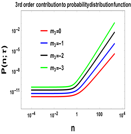
Refer to caption
(a) Fourth order corrected distribution for m4=0subscript𝑚40m_{4}=0
Refer to caption
(b) Fourth order corrected distribution for m4=±1subscript𝑚4plus-or-minus1m_{4}=\pm 1
Refer to caption
(c) Fourth order corrected distribution for m4=±2subscript𝑚4plus-or-minus2m_{4}=\pm 2
Refer to caption
(d) Fourth order corrected distribution for m4=±3subscript𝑚4plus-or-minus3m_{4}=\pm 3
Figure 43: Evolution of probability distribution function obtained from the fourth order corrected Fokker-Planck equation with the occupation number n𝑛n for different value of m4subscript𝑚4m_{4}. Here we use the initial conditions as mentioned in Eq (6.3.4).

During the analysis we assume that the particle production probability and all its derivative has a constant same value for n=0.0001𝑛0.0001n=0.0001, which is very very helpful for us to deal with the initial conditions during performing numerical techniques to solve the Eq (6.3.4).

From fig. 43 we observe that the fourth order corrected probability distribution function for different m4subscript𝑚4m_{4} is almost flat upto n=1𝑛1n=1 and after that the distribution function suddenly increases. Additionally, we observe that the fourth order correction has deviation from Gaussianity at small values of the occupation number. On the other hand, for large values of the occupation number we get a Gaussian like feature and that is shown explicitly in the mentioned plot.

Further using the Fourier transformation with respect to the occupation number n𝑛n as mentioned in Eq (655), we get the following simplified expression for the Fokker Planck equation at the fourth order:

4P¯(k;τ)τ4superscript4¯𝑃𝑘𝜏superscript𝜏4\displaystyle\frac{\partial^{4}\bar{P}(k;\tau)}{\partial\tau^{4}} =\displaystyle= μk4[70n4(1+n)4k8140in3(1+2n)k7\displaystyle\mu^{4}_{k}\left[70n^{4}(1+n)^{4}k^{8}-140in^{3}(1+2n)k^{7}\right. (749)
30n2(1+n)2(3+14n+14n2)k630superscript𝑛2superscript1𝑛2314𝑛14superscript𝑛2superscript𝑘6\displaystyle\left.-30n^{2}(1+n)^{2}(3+14n+14n^{2})k^{6}\right.
+20ni(1+n)(1+2n)(1+7n+7n2)k520𝑛𝑖1𝑛12𝑛17𝑛7superscript𝑛2superscript𝑘5\displaystyle\left.+20ni(1+n)(1+2n)(1+7n+7n^{2})k^{5}\right.
+(1+20n+90n2+140n3+70n4)k4]P¯(k;τ),\displaystyle\left.+(1+20n+90n^{2}+140n^{3}+70n^{4})k^{4}\right]\bar{P}(k;\tau),~{}~{}~{}~{}~{}~{}~{}~{}~{}~{}

which is obviously a simplest version of the Fokker Planck equation as it contains only four derivative with respect to time τ𝜏\tau. In the present context we get the following result for the probability distribution function in the Fourier transformed space, as given by:

P¯(k;τ|n;τ)¯𝑃𝑘conditional𝜏superscript𝑛superscript𝜏\displaystyle\bar{P}(k;\tau|n^{{}^{\prime}};\tau^{{}^{\prime}}) =\displaystyle= C1exp[𝒥(k;n)4(ττ)]+C2exp[𝒥(k;n)4(ττ)]subscript𝐶14𝒥𝑘superscript𝑛𝜏superscript𝜏subscript𝐶24𝒥𝑘superscript𝑛𝜏superscript𝜏\displaystyle C_{1}\exp\left[-\sqrt[4]{{\cal J}(k;n^{{}^{\prime}})}\left(\tau-\tau^{{}^{\prime}}\right)\right]+C_{2}\exp\left[\sqrt[4]{{\cal J}(k;n^{{}^{\prime}})}\left(\tau-\tau^{{}^{\prime}}\right)\right] (750)
+C3sin(𝒥(k;n)4(ττ))+C4cos(𝒥(k;n)4(ττ)),subscript𝐶34𝒥𝑘superscript𝑛𝜏superscript𝜏subscript𝐶44𝒥𝑘superscript𝑛𝜏superscript𝜏\displaystyle+C_{3}\sin\left(\sqrt[4]{{\cal J}(k;n^{{}^{\prime}})}\left(\tau-\tau^{{}^{\prime}}\right)\right)+C_{4}\cos\left(\sqrt[4]{{\cal J}(k;n^{{}^{\prime}})}\left(\tau-\tau^{{}^{\prime}}\right)\right),~{}~{}~{}~{}~{}~{}~{}~{}

where 𝒥(k;n)𝒥𝑘superscript𝑛{\cal J}(k;n^{{}^{\prime}}) is defined as:

𝒥(k;n)𝒥𝑘superscript𝑛\displaystyle{\cal J}(k;n^{{}^{\prime}}) =\displaystyle= μk4[70n4(1+n)4k8140in3(1+2n)k7\displaystyle\mu^{4}_{k}\left[70n^{{}^{\prime}4}(1+n^{{}^{\prime}})^{4}k^{8}-140in^{{}^{\prime}3}(1+2n^{{}^{\prime}})k^{7}\right. (751)
30n2(1+n)2(3+14n+14n2)k6\displaystyle\left.-30n^{2}(1+n^{{}^{\prime}})^{2}(3+14n^{{}^{\prime}}+14n^{{}^{\prime}2})k^{6}\right.
+20ni(1+n)(1+2n)(1+7n+7n2)k5\displaystyle\left.+20ni(1+n^{{}^{\prime}})(1+2n^{{}^{\prime}})(1+7n^{{}^{\prime}}+7n^{{}^{\prime}2})k^{5}\right.
+(1+20n+90n2+140n3+70n4)k4].\displaystyle\left.+(1+20n^{{}^{\prime}}+90n^{{}^{\prime}2}+140n^{{}^{\prime}3}+70n^{{}^{\prime}4})k^{4}\right].~{}~{}~{}~{}~{}~{}

Additionally, C1subscript𝐶1C_{1}, C2subscript𝐶2C_{2}, C3subscript𝐶3C_{3} and C4subscript𝐶4C_{4} are arbitrary constants which is fixed by the following three fold boundary conditions, as given by:

P(n;τ|n=0;τ=τ)\displaystyle P(n;\tau|n^{{}^{\prime}}=0;\tau^{{}^{\prime}}=\tau) =\displaystyle= δ(n),𝛿𝑛\displaystyle\delta(n), (752)
(P(n;τ|n;τ)τ)n=0,τ=τsubscript𝑃𝑛conditional𝜏superscript𝑛superscript𝜏𝜏formulae-sequencesuperscript𝑛0𝜏superscript𝜏\displaystyle\left(\frac{\partial P(n;\tau|n^{{}^{\prime}};\tau^{{}^{\prime}})}{\partial\tau}\right)_{n^{{}^{\prime}}=0,\tau=\tau^{{}^{\prime}}} =\displaystyle= δ(n)n,𝛿𝑛𝑛\displaystyle-\frac{\delta(n)}{n}, (753)
(2P(n;τ|n;τ)τ2)n=0,τ=τsubscriptsuperscript2𝑃𝑛conditional𝜏superscript𝑛superscript𝜏superscript𝜏2formulae-sequencesuperscript𝑛0𝜏superscript𝜏\displaystyle\left(\frac{\partial^{2}P(n;\tau|n^{{}^{\prime}};\tau^{{}^{\prime}})}{\partial\tau^{2}}\right)_{n^{{}^{\prime}}=0,\tau=\tau^{{}^{\prime}}} =\displaystyle= 2δ(n)n22𝛿𝑛superscript𝑛2\displaystyle\frac{2~{}\delta(n)}{n^{2}} (754)
(3P(n;τ|n;τ)τ3)n=0,τ=τsubscriptsuperscript3𝑃𝑛conditional𝜏superscript𝑛superscript𝜏superscript𝜏3formulae-sequencesuperscript𝑛0𝜏superscript𝜏\displaystyle\left(\frac{\partial^{3}P(n;\tau|n^{{}^{\prime}};\tau^{{}^{\prime}})}{\partial\tau^{3}}\right)_{n^{{}^{\prime}}=0,\tau=\tau^{{}^{\prime}}} =\displaystyle= 6δ(n)n3.6𝛿𝑛superscript𝑛3\displaystyle-\frac{6~{}\delta(n)}{n^{3}}. (755)

which are necessary to solve the above mentioned fourth order differential equation.

As a result, we get the following set of constraints equations:

C1+C2+C4=1,subscript𝐶1subscript𝐶2subscript𝐶41\displaystyle C_{1}+C_{2}+C_{4}=1, (756)
C1C2C3=1μkkn,subscript𝐶1subscript𝐶2subscript𝐶31subscript𝜇𝑘𝑘𝑛\displaystyle C_{1}-C_{2}-C_{3}=\frac{1}{\mu_{k}kn},~{}~{}~{}~{} (757)
C1+C2C3=2μk2k2n2,subscript𝐶1subscript𝐶2subscript𝐶32subscriptsuperscript𝜇2𝑘superscript𝑘2superscript𝑛2\displaystyle C_{1}+C_{2}-C_{3}=\frac{2}{\mu^{2}_{k}k^{2}n^{2}},~{}~{}~{}~{} (758)
C1C2+C3=6μk3k3n3.subscript𝐶1subscript𝐶2subscript𝐶36subscriptsuperscript𝜇3𝑘superscript𝑘3superscript𝑛3\displaystyle C_{1}-C_{2}+C_{3}=\frac{6}{\mu^{3}_{k}k^{3}n^{3}}. (759)

Solving these equations we get:

C1subscript𝐶1\displaystyle C_{1} =\displaystyle= k2n2μk22knμk64k3n3μk3,C2=k2n2μk22knμk+64k3n3μk3,superscript𝑘2superscript𝑛2superscriptsubscript𝜇𝑘22𝑘𝑛subscript𝜇𝑘64superscript𝑘3superscript𝑛3superscriptsubscript𝜇𝑘3subscript𝐶2superscript𝑘2superscript𝑛2superscriptsubscript𝜇𝑘22𝑘𝑛subscript𝜇𝑘64superscript𝑘3superscript𝑛3superscriptsubscript𝜇𝑘3\displaystyle\frac{-k^{2}n^{2}\mu_{k}^{2}-2kn\mu_{k}-6}{4k^{3}n^{3}\mu_{k}^{3}},~{}~{}~{}~{}~{}~{}C_{2}=-\frac{k^{2}n^{2}\mu_{k}^{2}-2kn\mu_{k}+6}{4k^{3}n^{3}\mu_{k}^{3}}, (760)
C3subscript𝐶3\displaystyle C_{3} =\displaystyle= k2n2μk262k3n3μk3,C4=1k2n2μk2.superscript𝑘2superscript𝑛2superscriptsubscript𝜇𝑘262superscript𝑘3superscript𝑛3superscriptsubscript𝜇𝑘3subscript𝐶41superscript𝑘2superscript𝑛2superscriptsubscript𝜇𝑘2\displaystyle-\frac{k^{2}n^{2}\mu_{k}^{2}-6}{2k^{3}n^{3}\mu_{k}^{3}},~{}~{}~{}~{}~{}~{}C_{4}=-\frac{1}{k^{2}n^{2}\mu_{k}^{2}}. (761)

Using this solution get the following probability distribution function in Fourier space, as given by:

P¯(k;τ)¯𝑃𝑘𝜏\displaystyle\bar{P}(k;\tau) =\displaystyle= k2n2μk22knμk64k3n3μk3exp[μkkτ]k2n2μk22knμk+64k3n3μk3exp[μkτ]superscript𝑘2superscript𝑛2superscriptsubscript𝜇𝑘22𝑘𝑛subscript𝜇𝑘64superscript𝑘3superscript𝑛3superscriptsubscript𝜇𝑘3subscript𝜇𝑘𝑘𝜏superscript𝑘2superscript𝑛2superscriptsubscript𝜇𝑘22𝑘𝑛subscript𝜇𝑘64superscript𝑘3superscript𝑛3superscriptsubscript𝜇𝑘3subscript𝜇𝑘𝜏\displaystyle\frac{-k^{2}n^{2}\mu_{k}^{2}-2kn\mu_{k}-6}{4k^{3}n^{3}\mu_{k}^{3}}~{}\exp\left[-\mu_{k}k\tau\right]-\frac{k^{2}n^{2}\mu_{k}^{2}-2kn\mu_{k}+6}{4k^{3}n^{3}\mu_{k}^{3}}~{}\exp\left[\mu_{k}\tau\right] (762)
k2n2μk262k3n3μk3sin(μkkτ)1k2n2μk2cos(μkkτ),superscript𝑘2superscript𝑛2superscriptsubscript𝜇𝑘262superscript𝑘3superscript𝑛3superscriptsubscript𝜇𝑘3subscript𝜇𝑘𝑘𝜏1superscript𝑘2superscript𝑛2superscriptsubscript𝜇𝑘2subscript𝜇𝑘𝑘𝜏\displaystyle-\frac{k^{2}n^{2}\mu_{k}^{2}-6}{2k^{3}n^{3}\mu_{k}^{3}}\sin\left(\mu_{k}k\tau\right)-\frac{1}{k^{2}n^{2}\mu_{k}^{2}}\cos\left(\mu_{k}k\tau\right),~{}~{}~{}~{}~{}~{}~{}~{}

Hence substituting back into the definition of Fourier transformation and setting the initial condition n=0superscript𝑛0n^{{}^{\prime}}=0 and τ=0superscript𝜏0\tau^{{}^{\prime}}=0 we get the following result for the probability distribution function, as given by:

P(n;τ)𝑃𝑛𝜏\displaystyle P(n;\tau) =\displaystyle= 12πdkexp[ikn]{k2n2μk22knμk64k3n3μk3exp[μkkτ]\displaystyle\frac{1}{2\pi}\int^{\infty}_{-\infty}dk~{}\exp\left[ikn\right]\left\{\frac{-k^{2}n^{2}\mu_{k}^{2}-2kn\mu_{k}-6}{4k^{3}n^{3}\mu_{k}^{3}}~{}\exp\left[-\mu_{k}k\tau\right]\right. (763)
k2n2μk22knμk+64k3n3μk3exp[μkτ]superscript𝑘2superscript𝑛2superscriptsubscript𝜇𝑘22𝑘𝑛subscript𝜇𝑘64superscript𝑘3superscript𝑛3superscriptsubscript𝜇𝑘3subscript𝜇𝑘𝜏\displaystyle\left.~{}~{}~{}~{}~{}~{}~{}~{}~{}~{}~{}~{}~{}~{}~{}~{}~{}~{}-\frac{k^{2}n^{2}\mu_{k}^{2}-2kn\mu_{k}+6}{4k^{3}n^{3}\mu_{k}^{3}}~{}\exp\left[\mu_{k}\tau\right]\right.
k2n2μk262k3n3μk3sin(μkkτ)1k2n2μk2cos(μkkτ)}\displaystyle\left.~{}~{}~{}~{}~{}~{}~{}~{}~{}~{}~{}~{}~{}~{}~{}~{}~{}~{}-\frac{k^{2}n^{2}\mu_{k}^{2}-6}{2k^{3}n^{3}\mu_{k}^{3}}\sin\left(\mu_{k}k\tau\right)-\frac{1}{k^{2}n^{2}\mu_{k}^{2}}\cos\left(\mu_{k}k\tau\right)\right\}

which is divergent within the interval <k<𝑘-\infty<k<\infty. After introducing an IR and UV regulators, Q<k<L𝑄𝑘𝐿Q<k<L we can get a finite result, which we have not presented in this paper for its huge length. The origin of such corrections are the fourth order contribution in the Fokker Planck equation.
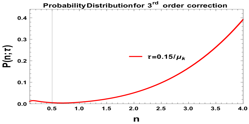
Refer to caption
Figure 44: Fourth order contribution to the probability density function with respect to the the occupation number per mode n𝑛n, for a fixed time from the analytical solution [Eq:-763] of the fourth order correction distribution function[Eq:-6.3.4].

In Fig:-44, we have shown the fourth order correction to the probability density function with respect to the occupation number per mode, for a fixed time (μkτsubscript𝜇𝑘𝜏\mu_{k}\tau=fixed) flow the intial gaussian then exponential decay type distribution.This decreasing feature suggest very low effect from fourth order correction which is also supported by perturbative expansion assumption.

6.3.5 Total solution considering different order correction

Now we plot total solutions with different order of correction with main solution.Then we check validation of different order of correction altogether and how they merge with each other at what limit.
A. Upto second order correction:-
Further we consider upto second order corrected solution with first order contribution at m1=2subscript𝑚12m_{1}=2 for different m2subscript𝑚2m_{2}.

Refer to caption
(a) Upto second order corrected distribution for m2=1subscript𝑚21m_{2}=1
Refer to caption
(b) Upto second order corrected distribution for m2=0subscript𝑚20m_{2}=0
Refer to caption
(c) second order analytic solution
Figure 45: Second order corrected probability distribution profile for different m2subscript𝑚2m_{2} with previously mentioned initial conditions. Here we fix m=2𝑚2m=2. Here the subscript 111 and 222 stands for the corrected order in the distribution.

From Fig:-45(a),45(b) we observe that at low values of n𝑛n, P1+P2subscript𝑃1subscript𝑃2P_{1}+P_{2} and P2subscript𝑃2P_{2} are significantly different, but as we increase n𝑛n they overlapped and P2subscript𝑃2P_{2} effect is more over P1+P2subscript𝑃1subscript𝑃2P_{1}+P_{2} so the second order solution dominate over the first order solution.On the other hand Fig:-45(c) shows how the second order contribution effect the primary gaussian curve. Distinct oscillation effect on gaussian curve shows the effect of second order correction which is not available from the numerical solution.

B. Upto third order correction:-

Here we add all the three previously derived contributions to produce the total probability distribution corrected upto third order.
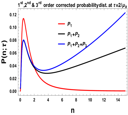
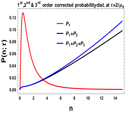
Refer to caption
(a) upto third order corrected distribution for m3=0subscript𝑚30m_{3}=0,m2=0subscript𝑚20m_{2}=0
Refer to caption
(b) Upto third order corrected distribution for m2=0subscript𝑚20m_{2}=0 and m3=1subscript𝑚31m_{3}=1.
Refer to caption
(c) upto third order corrected analytical solution
Refer to caption
(d) comparison between 2nd order and third order effect
Figure 46: Upto third order corrected probability distribution profile for different m3subscript𝑚3m_{3},m2subscript𝑚2m_{2} and m1=2subscript𝑚12m_{1}=2 with previously mentioned initial conditions and Exact analytical solution for probability distribution with previous correction included

From fig. 46(a),46(b) we observe that P1+P2+P3subscript𝑃1subscript𝑃2subscript𝑃3P_{1}+P_{2}+P_{3}, P2+P3subscript𝑃2subscript𝑃3P_{2}+P_{3} and P3subscript𝑃3P_{3} overlap at higher n𝑛n limit though separated. At low n𝑛n limit and P1+P2subscript𝑃1subscript𝑃2P_{1}+P_{2} and P2subscript𝑃2P_{2} overlap with each other but remain separated from P1+P2+P3subscript𝑃1subscript𝑃2subscript𝑃3P_{1}+P_{2}+P_{3} for the complete range. This implies that third order contribution is dominant over the other two due to the non-linearities in the differential equation and behaves like a non-perturbative quantum effect at the level of solution. From fig 46(c) we show the third order correction affects the tail of the gaussian and shift it bit higher.It is clear from fig 46(d).
C. Upto fourth order correction:-
Here we add all the four previously derived contributions to produce the total probability distribution corrected upto fourth order.
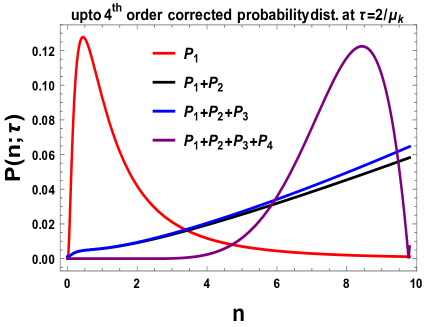
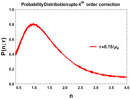
Refer to caption
(a) upto fourth order corrected solution for different m1subscript𝑚1m_{1},m2subscript𝑚2m_{2},m3subscript𝑚3m_{3} and m4subscript𝑚4m_{4}
Refer to caption
(b) Upto 4th order correction
Refer to caption
(c) Upto 4th order correction
Refer to caption
(d) Upto 4th order correction comparison between different correction
Figure 47: Fourth order corrected probability distribution for different m4subscript𝑚4m_{4},m3subscript𝑚3m_{3},m2subscript𝑚2m_{2} and m1=2subscript𝑚12m_{1}=2 with previously mentioned initial conditions.

From fig. 47(a) we observe the final curve represented by P1+P2+P3+P4subscript𝑃1subscript𝑃2subscript𝑃3subscript𝑃4P_{1}+P_{2}+P_{3}+P_{4} shifted the mean of the gaussian from its value at P1subscript𝑃1P_{1}.Initial gaussian feature for P1+P2+P3subscript𝑃1subscript𝑃2subscript𝑃3P_{1}+P_{2}+P_{3} and P1+P2subscript𝑃1subscript𝑃2P_{1}+P_{2} are deviated at high n𝑛n limit . Here P1+P2+P3+P4subscript𝑃1subscript𝑃2subscript𝑃3subscript𝑃4P_{1}+P_{2}+P_{3}+P_{4} and P1subscript𝑃1P_{1} follow exact gaussian nature but they are mirror image of one another. P1+P2+P3subscript𝑃1subscript𝑃2subscript𝑃3P_{1}+P_{2}+P_{3} and P1+P2subscript𝑃1subscript𝑃2P_{1}+P_{2} don’t have this gaussian nature due to their divergence property as n increases. In fig 47(b) and fig 47(c) the effect of all order correction can be observed but effect of different order correction become evident from fig 47(d).Second order correction introduce the oscillating feature whereas third order correction increase the tail and responsible for higher kurtosis. Fourth order correction add a small positive effect to the previous correction without any shape change.

Previously it is shown that in ref. Amin:2015ftc the distribution will be log-normal at large n𝑛n, considering the lowest order contribution coming from the solution of Fokker-Planck equation. We extend this result upto fourth order and shown the effect of different order correction.The oscillating nature and long tail can be specific feature of stochastic particle production in inflation epoch.This may be the effect of background field or noise at that time.The numerical solutions give different quantum numbers which support the quantum nature. In the next subsection we will calculate various statistical moments and from that we can discuss about the role of quantum effects and non-Gaussinanity from the Probability distribution profile for particle production in the context of early universe cosmology (mostly during reheating).

6.4 Calculation of statistical moments (or quantum correlation functions) from corrected probability distribution function

Here our prime objective is to compute the different statistical moments from the quantum corrected probability distribution function as obtain by Taylor expanding in order by order from Eq (587). From is corrected probability distribution function we compute the expression for ndelimited-⟨⟩𝑛\langle n\rangle,n2delimited-⟨⟩superscript𝑛2\langle n^{2}\rangle,n3delimited-⟨⟩superscript𝑛3\langle n^{3}\rangle and n4delimited-⟨⟩superscript𝑛4\langle n^{4}\rangle and then calculate standard deviation, skewness and kurtosis for a given time. We have explicitly shown that the non vanishing contributions of skewness and kurtosis carries the signature of significant effect of non-Gaussianity. In this analysis the values of these moments are compared with predicted results obtained from log-normal (Gaussian) distribution and non zero values of kurtosis and skewness define the deviation from that.

To compute the moments we start with the following sets of master evolution equations valid in different orders, as given by:

𝐅𝐢𝐫𝐬𝐭𝐎𝐫𝐝𝐞𝐫𝐌𝐚𝐬𝐭𝐞𝐫𝐄𝐯𝐨𝐥𝐮𝐭𝐢𝐨𝐧𝐄𝐪𝐮𝐚𝐭𝐢𝐨𝐧:¯¯:𝐅𝐢𝐫𝐬𝐭𝐎𝐫𝐝𝐞𝐫𝐌𝐚𝐬𝐭𝐞𝐫𝐄𝐯𝐨𝐥𝐮𝐭𝐢𝐨𝐧𝐄𝐪𝐮𝐚𝐭𝐢𝐨𝐧absent\displaystyle{\color[rgb]{0,0,1}\bf\underline{First~{}Order~{}Master~{}Evolution~{}Equation:}}~{}~{}~{}~{}~{}~{}~{}~{}~{}
1μkFτ=(1+2n)Fn+n(n+1)2Fn2,1subscript𝜇𝑘delimited-⟨⟩𝐹𝜏delimited-⟨⟩12𝑛𝐹𝑛𝑛𝑛1superscript2𝐹superscript𝑛2\displaystyle~{}~{}~{}~{}~{}~{}~{}~{}~{}~{}~{}~{}~{}~{}~{}~{}~{}~{}~{}~{}~{}~{}~{}~{}~{}~{}~{}~{}\frac{1}{\mu_{k}}\frac{\partial\langle F\rangle}{\partial\tau}=\left\langle(1+2n)\frac{\partial F}{\partial n}+n(n+1)\frac{\partial^{2}F}{\partial n^{2}}\right\rangle, (764)
𝐒𝐞𝐜𝐨𝐧𝐝𝐎𝐫𝐝𝐞𝐫𝐌𝐚𝐬𝐭𝐞𝐫𝐄𝐯𝐨𝐥𝐮𝐭𝐢𝐨𝐧𝐄𝐪𝐮𝐚𝐭𝐢𝐨𝐧:¯¯:𝐒𝐞𝐜𝐨𝐧𝐝𝐎𝐫𝐝𝐞𝐫𝐌𝐚𝐬𝐭𝐞𝐫𝐄𝐯𝐨𝐥𝐮𝐭𝐢𝐨𝐧𝐄𝐪𝐮𝐚𝐭𝐢𝐨𝐧absent\displaystyle{\color[rgb]{0,0,1}\bf\underline{Second~{}Order~{}Master~{}Evolution~{}Equation:}}~{}~{}~{}~{}~{}~{}~{}~{}~{}
1μk22Fτ2=n22(1+n)24Fn4+2n(1+3n+2n2)3Fn3+(1+6n+6n2)2Fn2,1subscriptsuperscript𝜇2𝑘superscript2delimited-⟨⟩𝐹superscript𝜏2delimited-⟨⟩superscript𝑛22superscript1𝑛2superscript4𝐹superscript𝑛42𝑛13𝑛2superscript𝑛2superscript3𝐹superscript𝑛316𝑛6superscript𝑛2superscript2𝐹superscript𝑛2\displaystyle~{}~{}~{}~{}~{}~{}\frac{1}{\mu^{2}_{k}}\frac{\partial^{2}\langle F\rangle}{\partial\tau^{2}}=\left\langle\frac{n^{2}}{2}\left(1+n\right)^{2}\frac{\partial^{4}F}{\partial n^{4}}+2n\left(1+3n+2n^{2}\right)\frac{\partial^{3}F}{\partial n^{3}}+\left(1+6n+6n^{2}\right)\frac{\partial^{2}F}{\partial n^{2}}\right\rangle,~{}~{}~{}~{}~{}~{}~{}~{}~{}~{}~{}~{} (765)
𝐓𝐡𝐢𝐫𝐝𝐎𝐫𝐝𝐞𝐫𝐌𝐚𝐬𝐭𝐞𝐫𝐄𝐯𝐨𝐥𝐮𝐭𝐢𝐨𝐧𝐄𝐪𝐮𝐚𝐭𝐢𝐨𝐧:¯¯:𝐓𝐡𝐢𝐫𝐝𝐎𝐫𝐝𝐞𝐫𝐌𝐚𝐬𝐭𝐞𝐫𝐄𝐯𝐨𝐥𝐮𝐭𝐢𝐨𝐧𝐄𝐪𝐮𝐚𝐭𝐢𝐨𝐧absent\displaystyle{\color[rgb]{0,0,1}\bf\underline{Third~{}Order~{}Master~{}Evolution~{}Equation:}}~{}~{}~{}~{}~{}~{}~{}~{}~{}
1μk33Fτ3=n36(1+n)36Fn6+3n22(1+n)2(1+2n)5Fn5\displaystyle~{}~{}~{}~{}~{}~{}\frac{1}{\mu^{3}_{k}}\frac{\partial^{3}\langle F\rangle}{\partial\tau^{3}}=\left\langle\frac{n^{3}}{6}(1+n)^{3}\frac{\partial^{6}F}{\partial n^{6}}+\frac{3n^{2}}{2}(1+n)^{2}(1+2n)\frac{\partial^{5}F}{\partial n^{5}}\right.
+3n(1+n)(1+5n+5n2)4Fn4+(1+2n)(1+10n+10n2)3Fn3,\displaystyle\left.~{}~{}~{}~{}~{}~{}~{}~{}~{}~{}~{}~{}~{}~{}~{}~{}~{}~{}~{}~{}+3n(1+n)(1+5n+5n^{2})\frac{\partial^{4}F}{\partial n^{4}}+(1+2n)(1+10n+10n^{2})\frac{\partial^{3}F}{\partial n^{3}}\right\rangle,~{}~{}~{}~{}~{}~{}~{}~{}~{}~{}~{}~{} (766)
𝐅𝐨𝐮𝐫𝐭𝐡𝐎𝐫𝐝𝐞𝐫𝐌𝐚𝐬𝐭𝐞𝐫𝐄𝐯𝐨𝐥𝐮𝐭𝐢𝐨𝐧𝐄𝐪𝐮𝐚𝐭𝐢𝐨𝐧:¯¯:𝐅𝐨𝐮𝐫𝐭𝐡𝐎𝐫𝐝𝐞𝐫𝐌𝐚𝐬𝐭𝐞𝐫𝐄𝐯𝐨𝐥𝐮𝐭𝐢𝐨𝐧𝐄𝐪𝐮𝐚𝐭𝐢𝐨𝐧absent\displaystyle{\color[rgb]{0,0,1}\bf\underline{Fourth~{}Order~{}Master~{}Evolution~{}Equation:}}~{}~{}~{}~{}~{}~{}~{}~{}~{}
1μk44Fτ4=70n4(1+n)48Fn8+140n3(1+2n)7Fn7\displaystyle~{}~{}~{}~{}~{}~{}\frac{1}{\mu^{4}_{k}}\frac{\partial^{4}\langle F\rangle}{\partial\tau^{4}}=\left\langle 70n^{4}(1+n)^{4}\frac{\partial^{8}F}{\partial n^{8}}+140n^{3}(1+2n)\frac{\partial^{7}F}{\partial n^{7}}\right.
+30n2(1+n)2(3+14n+14n2)6Fn630superscript𝑛2superscript1𝑛2314𝑛14superscript𝑛2superscript6𝐹superscript𝑛6\displaystyle~{}~{}~{}~{}~{}~{}~{}~{}~{}~{}~{}~{}~{}~{}~{}~{}~{}~{}~{}~{}~{}~{}~{}~{}~{}\left.+30n^{2}(1+n)^{2}(3+14n+14n^{2})\frac{\partial^{6}F}{\partial n^{6}}\right.
+20n(1+n)(1+2n)(1+7n+7n2)5Fn520𝑛1𝑛12𝑛17𝑛7superscript𝑛2superscript5𝐹superscript𝑛5\displaystyle~{}~{}~{}~{}~{}~{}~{}~{}~{}~{}~{}~{}~{}~{}~{}~{}~{}~{}~{}~{}~{}~{}~{}~{}~{}\left.+20n(1+n)(1+2n)(1+7n+7n^{2})\frac{\partial^{5}F}{\partial n^{5}}\right.
+(1+20n+90n2+140n3+70n4)4Fn4,.\displaystyle~{}~{}~{}~{}~{}~{}~{}~{}~{}~{}~{}~{}~{}~{}~{}~{}~{}~{}~{}~{}~{}~{}~{}~{}~{}\left.+(1+20n+90n^{2}+140n^{3}+70n^{4})\frac{\partial^{4}F}{\partial n^{4}}\right\rangle,~{}~{}~{}~{}~{}~{}~{}~{}~{}~{}~{}~{}. (767)

where the first moment or the expectation value of the observable F𝐹F is define as:

𝐅𝐢𝐫𝐬𝐭𝐌𝐨𝐦𝐞𝐧𝐭:¯F(n)(τ)𝑑nF(n)P(n;τ).¯:𝐅𝐢𝐫𝐬𝐭𝐌𝐨𝐦𝐞𝐧𝐭absentdelimited-⟨⟩𝐹𝑛𝜏differential-d𝑛𝐹𝑛𝑃𝑛𝜏{\color[rgb]{0,0,1}\bf\underline{First~{}Moment:}}~{}~{}~{}~{}~{}~{}\langle F(n)\rangle(\tau)\equiv\int~{}dn~{}F(n)P(n;\tau)~{}. (768)

Here F(n)𝐹𝑛F(n) is the physical observable in which we are interested in and P(n;τ)𝑃𝑛𝜏P(n;\tau) is the corrected probability distribution function which is not necessarily log-normal (Gaussian) in nature. In the present context of discussion, Eq (768) plays the role of generating function, which is commonly used in calculating various mathematical special functions. In our discussion, Eq (768) represents the statistical moment generating function in presence of quantum corrected probability distribution function. In terms of quantum mechanical language, Eq (768) signify the one point quantum correlation function and it is exactly equal to the statistical first moment in this discussion.

Now, we explicitly compute the expressions for one point function (or first moment) of the occupation number i.e. ndelimited-⟨⟩𝑛\langle n\rangle, two point function (or second moment) of the occupation number i.e. n2delimited-⟨⟩superscript𝑛2\langle n^{2}\rangle, three point function (or third moment) of the occupation number i.e. n3delimited-⟨⟩superscript𝑛3\langle n^{3}\rangle and four point function (or fourth moment) of the occupation number i.e. n2delimited-⟨⟩superscript𝑛2\langle n^{2}\rangle using the previously mentioned first, second, third and fourth order master equations. The detailed steps of the computations are appended bellow:

  1. 1.

    Step I:
    First of all, we use the first order master evolution equation. Then we replace the function F𝐹F by the occupation number n𝑛n. Consequently, we get the following time evolution equation of the first moment or one point function ndelimited-⟨⟩𝑛\langle n\rangle, given by:

    1μknτ=(1+2n)=1+2n.1subscript𝜇𝑘delimited-⟨⟩𝑛𝜏delimited-⟨⟩12𝑛12delimited-⟨⟩𝑛\displaystyle\frac{1}{\mu_{k}}\frac{\partial\langle n\rangle}{\partial\tau}=\langle(1+2n)\rangle=1+2\langle n\rangle~{}. (769)
  2. 2.

    Step II:
    Secondly, we want to compute the expression for n2delimited-⟨⟩superscript𝑛2\langle n^{2}\rangle. To compute this we consider here the first and second order master equations, as mentioned earlier. Considering only the first order master equation we get the following analytical expression:

    1μkn2τ=2n(1+2n)+2n(1+n)=4n+6n2=4n+6n2.1subscript𝜇𝑘delimited-⟨⟩superscript𝑛2𝜏delimited-⟨⟩2𝑛12𝑛2𝑛1𝑛delimited-⟨⟩4𝑛6superscript𝑛24delimited-⟨⟩𝑛6delimited-⟨⟩superscript𝑛2\displaystyle\frac{1}{\mu_{k}}\frac{\partial\langle n^{2}\rangle}{\partial\tau}=\langle 2n(1+2n)+2n(1+n)\rangle=\langle 4n+6n^{2}\rangle=4\langle n\rangle+6\langle n^{2}\rangle~{}. (770)

    On the other hand, using the second order master equation we get the following analytical expression for the time evolution of the second moment or two point correlation:

    1μk22n2τ2=2(1+6n+6n2)=12n+12n2+2.1superscriptsubscript𝜇𝑘2superscript2delimited-⟨⟩superscript𝑛2superscript𝜏2delimited-⟨⟩216𝑛6superscript𝑛212delimited-⟨⟩𝑛12delimited-⟨⟩superscript𝑛22\frac{1}{\mu_{k}^{2}}\frac{\partial^{2}\langle n^{2}\rangle}{\partial\tau^{2}}=\langle 2(1+6n+6n^{2})\rangle=12\langle n\rangle+12\langle n^{2}\rangle+2~{}. (771)
  3. 3.

    Step III:
    Next, we want to compute the expression for n3delimited-⟨⟩superscript𝑛3\langle n^{3}\rangle. To compute this we consider here the first, second and third order master equations, as mentioned earlier. Considering only the first order master equation we get the following analytical expression:

    1μkn3τ=3n2(1+2n)+6n(1+n)=6n+9n2+6n3=6n+9n2+6n3.1subscript𝜇𝑘delimited-⟨⟩superscript𝑛3𝜏delimited-⟨⟩3superscript𝑛212𝑛6𝑛1𝑛delimited-⟨⟩6𝑛9superscript𝑛26superscript𝑛36delimited-⟨⟩𝑛9delimited-⟨⟩superscript𝑛26delimited-⟨⟩superscript𝑛3\frac{1}{\mu_{k}}\frac{\partial\langle n^{3}\rangle}{\partial\tau}=\langle 3n^{2}(1+2n)+6n(1+n)\rangle=\langle 6n+9n^{2}+6n^{3}\rangle=6\langle n\rangle+9\langle n^{2}\rangle+6\langle n^{3}\rangle~{}. (772)

    On the other hand, using the second order master equation we get the following analytical expression for the time evolution of the third moment or three point correlation:

    1μk22n3τ2=12n(1+3n+3n2)+6n(1+6n+6n2)=18n+72n2+60n3.1superscriptsubscript𝜇𝑘2superscript2delimited-⟨⟩superscript𝑛3superscript𝜏2delimited-⟨⟩12𝑛13𝑛3superscript𝑛26𝑛16𝑛6superscript𝑛218delimited-⟨⟩𝑛72delimited-⟨⟩superscript𝑛260delimited-⟨⟩superscript𝑛3\frac{1}{\mu_{k}^{2}}\frac{\partial^{2}\langle n^{3}\rangle}{\partial\tau^{2}}=\langle 12n(1+3n+3n^{2})+6n(1+6n+6n^{2})\rangle=18\langle n\rangle+72\langle n^{2}\rangle+60\langle n^{3}\rangle~{}. (773)

    Finally, using the third order master equation we get the following analytical expression for the time evolution of the third moment or three point correlation:

    1μk33n3τ3=6(1+2n)(1+10n+10n2)=72n+180n2+120n3+6.1superscriptsubscript𝜇𝑘3superscript3delimited-⟨⟩superscript𝑛3superscript𝜏3delimited-⟨⟩612𝑛110𝑛10superscript𝑛272delimited-⟨⟩𝑛180delimited-⟨⟩superscript𝑛2120delimited-⟨⟩superscript𝑛36\frac{1}{\mu_{k}^{3}}\frac{\partial^{3}\langle n^{3}\rangle}{\partial\tau^{3}}=\langle 6(1+2n)(1+10n+10n^{2})\rangle=72\langle n\rangle+180\langle n^{2}\rangle+120\langle n^{3}\rangle+6~{}. (774)
  4. 4.

    Step IV:
    Next, we want to compute the expression for n4delimited-⟨⟩superscript𝑛4\langle n^{4}\rangle. To compute this we consider here the first, second, third and fourth order master equations, as mentioned earlier. Considering only the first order master equation we get the following analytical expression:

    1μkn4τ1subscript𝜇𝑘delimited-⟨⟩superscript𝑛4𝜏\displaystyle\frac{1}{\mu_{k}}\frac{\partial\langle n^{4}\rangle}{\partial\tau} =\displaystyle= 4n3(1+2n)+12n2(1+n)=16n3+20n4=16n3+20n4.delimited-⟨⟩4superscript𝑛312𝑛12superscript𝑛21𝑛delimited-⟨⟩16superscript𝑛320superscript𝑛416delimited-⟨⟩superscript𝑛320delimited-⟨⟩superscript𝑛4\displaystyle\langle 4n^{3}(1+2n)+12n^{2}(1+n)\rangle=\langle 16n^{3}+20n^{4}\rangle=16\langle n^{3}\rangle+20\langle n^{4}\rangle~{}.~{}~{}~{}~{}~{}~{} (775)

    On the other hand, using the second order master equation we get the following analytical expression for the time evolution of the fourth moment or four point correlation:

    1μk22n4τ21superscriptsubscript𝜇𝑘2superscript2delimited-⟨⟩superscript𝑛4superscript𝜏2\displaystyle\frac{1}{\mu_{k}^{2}}\frac{\partial^{2}\langle n^{4}\rangle}{\partial\tau^{2}} =\displaystyle= 12n2(1+n)2+48n2(1+3n+2n2)+12n2(1+6n+6n2)delimited-⟨⟩12superscript𝑛2superscript1𝑛248superscript𝑛213𝑛2superscript𝑛212superscript𝑛216𝑛6superscript𝑛2\displaystyle\langle 12n^{2}(1+n)^{2}+48n^{2}(1+3n+2n^{2})+12n^{2}(1+6n+6n^{2})\rangle (776)
    =\displaystyle= 72n2+240n3+180n4.72delimited-⟨⟩superscript𝑛2240delimited-⟨⟩superscript𝑛3180delimited-⟨⟩superscript𝑛4\displaystyle 72\langle n^{2}\rangle+240\langle n^{3}\rangle+180\langle n^{4}\rangle~{}.

    Then, using the third order master equation we get the following analytical expression for the time evolution of the fourth moment or fourth point correlation:

    1μk33n4τ31superscriptsubscript𝜇𝑘3superscript3delimited-⟨⟩superscript𝑛4superscript𝜏3\displaystyle\frac{1}{\mu_{k}^{3}}\frac{\partial^{3}\langle n^{4}\rangle}{\partial\tau^{3}} =\displaystyle= 72n(1+n)(1+5n+5n2)+24n(1+2n)(1+10n+10n2)delimited-⟨⟩72𝑛1𝑛15𝑛5superscript𝑛224𝑛12𝑛110𝑛10superscript𝑛2\displaystyle\langle 72n(1+n)(1+5n+5n^{2})+24n(1+2n)(1+10n+10n^{2})\rangle (777)
    =\displaystyle= 96n+720n2+1440n3+840n4.96delimited-⟨⟩𝑛720delimited-⟨⟩superscript𝑛21440delimited-⟨⟩superscript𝑛3840delimited-⟨⟩superscript𝑛4\displaystyle 96\langle n\rangle+720\langle n^{2}\rangle+1440\langle n^{3}\rangle+840\langle n^{4}\rangle~{}.

    Finally, using the third order master equation we get the following analytical expression for the time evolution of the fourth moment or fourth point correlation:

    1μk44n4τ41superscriptsubscript𝜇𝑘4superscript4delimited-⟨⟩superscript𝑛4superscript𝜏4\displaystyle\frac{1}{\mu_{k}^{4}}\frac{\partial^{4}\langle n^{4}\rangle}{\partial\tau^{4}} =\displaystyle= 24(1+20n+90n2+140n3+70n4)delimited-⟨⟩24120𝑛90superscript𝑛2140superscript𝑛370superscript𝑛4\displaystyle\langle 24(1+20n+90n^{2}+140n^{3}+70n^{4})\rangle (778)
    =\displaystyle= 480n+2160n2+3360n3+1680n4+24.480delimited-⟨⟩𝑛2160delimited-⟨⟩superscript𝑛23360delimited-⟨⟩superscript𝑛31680delimited-⟨⟩superscript𝑛424\displaystyle 480\langle n\rangle+2160\langle n^{2}\rangle+3360\langle n^{3}\rangle+1680\langle n^{4}\rangle+24~{}.
  5. 5.

    Step V:
    Further we apply the boundary conditions, i.e. ndelimited-⟨⟩𝑛\langle n\rangle, n2delimited-⟨⟩superscript𝑛2\langle n^{2}\rangle, n3delimited-⟨⟩superscript𝑛3\langle n^{3}\rangle, n4delimited-⟨⟩superscript𝑛4\langle n^{4}\rangle, dn2dτ2𝑑delimited-⟨⟩superscript𝑛2𝑑superscript𝜏2\frac{d\langle n^{2}\rangle}{d\tau^{2}}, dn3dτ3𝑑delimited-⟨⟩superscript𝑛3𝑑superscript𝜏3\frac{d\langle n^{3}\rangle}{d\tau^{3}} and , dn4dτ4𝑑delimited-⟨⟩superscript𝑛4𝑑superscript𝜏4\frac{d\langle n^{4}\rangle}{d\tau^{4}} are vanishingly small at τ=0𝜏0\tau=0. Using these conditions we get expressions for ndelimited-⟨⟩𝑛\langle n\rangle, n2delimited-⟨⟩superscript𝑛2\langle n^{2}\rangle, n3delimited-⟨⟩superscript𝑛3\langle n^{3}\rangle and n4delimited-⟨⟩superscript𝑛4\langle n^{4}\rangle.

  6. 6.

    Step VI:
    Using the result obtained in Step I and using the previously mentioned boundary condition we get the following expression for the one point function 313131Here it is important to note that as far as quantum mechanical computation is concerned, it produces same result for the one point function and first moment of the occupation number and both of them is equal to the expectation or average value of the occupation number in this context. (or first moment) of occupation number:

    𝐅𝐢𝐫𝐬𝐭𝐌𝐨𝐦𝐞𝐧𝐭(𝐅𝐢𝐫𝐬𝐭𝐎𝐫𝐝𝐞𝐫):¯n𝐈=12(e2τμk1).¯:𝐅𝐢𝐫𝐬𝐭𝐌𝐨𝐦𝐞𝐧𝐭𝐅𝐢𝐫𝐬𝐭𝐎𝐫𝐝𝐞𝐫absentsubscriptdelimited-⟨⟩𝑛𝐈12superscript𝑒2𝜏subscript𝜇𝑘1\displaystyle{\color[rgb]{0,0,1}\bf\underline{First~{}Moment~{}(First~{}Order):}}~{}~{}~{}~{}~{}~{}~{}~{}~{}\langle n\rangle_{{\color[rgb]{1,0,0}\bf I}}=\frac{1}{2}(e^{2\tau\mu_{k}}-1)~{}. (779)

    which is further used to compute all the higher order moments from master evolution equation considering higher order Taylor expansion. Additionally, it is important to note that if we use higher order equations for the first moment then after imposing the boundary conditions we get the following results:

    𝐅𝐢𝐫𝐬𝐭𝐌𝐨𝐦𝐞𝐧𝐭(𝐒𝐞𝐜𝐨𝐧𝐝𝐎𝐫𝐝𝐞𝐫):¯n𝐈𝐈=0,¯:𝐅𝐢𝐫𝐬𝐭𝐌𝐨𝐦𝐞𝐧𝐭𝐒𝐞𝐜𝐨𝐧𝐝𝐎𝐫𝐝𝐞𝐫absentsubscriptdelimited-⟨⟩𝑛𝐈𝐈0\displaystyle{\color[rgb]{0,0,1}\bf\underline{First~{}Moment~{}(Second~{}Order):}}~{}~{}~{}~{}~{}~{}~{}~{}~{}\langle n\rangle_{{\color[rgb]{1,0,0}\bf II}}=0, (780)
    𝐅𝐢𝐫𝐬𝐭𝐌𝐨𝐦𝐞𝐧𝐭(𝐓𝐡𝐢𝐫𝐝𝐎𝐫𝐝𝐞𝐫):¯n𝐈𝐈𝐈=0,¯:𝐅𝐢𝐫𝐬𝐭𝐌𝐨𝐦𝐞𝐧𝐭𝐓𝐡𝐢𝐫𝐝𝐎𝐫𝐝𝐞𝐫absentsubscriptdelimited-⟨⟩𝑛𝐈𝐈𝐈0\displaystyle{\color[rgb]{0,0,1}\bf\underline{First~{}Moment~{}(Third~{}Order):}}~{}~{}~{}~{}~{}~{}~{}~{}~{}\langle n\rangle_{{\color[rgb]{1,0,0}\bf III}}=0, (781)
    𝐅𝐢𝐫𝐬𝐭𝐌𝐨𝐦𝐞𝐧𝐭(𝐅𝐨𝐮𝐫𝐭𝐡𝐎𝐫𝐝𝐞𝐫):¯n𝐈𝐕=0.¯:𝐅𝐢𝐫𝐬𝐭𝐌𝐨𝐦𝐞𝐧𝐭𝐅𝐨𝐮𝐫𝐭𝐡𝐎𝐫𝐝𝐞𝐫absentsubscriptdelimited-⟨⟩𝑛𝐈𝐕0\displaystyle{\color[rgb]{0,0,1}\bf\underline{First~{}Moment~{}(Fourth~{}Order):}}~{}~{}~{}~{}~{}~{}~{}~{}~{}\langle n\rangle_{{\color[rgb]{1,0,0}\bf IV}}=0~{}. (782)

    Consequently, the total first moment can be written as:

    𝐓𝐨𝐭𝐚𝐥𝐅𝐢𝐫𝐬𝐭𝐌𝐨𝐦𝐞𝐧𝐭:¯n¯:𝐓𝐨𝐭𝐚𝐥𝐅𝐢𝐫𝐬𝐭𝐌𝐨𝐦𝐞𝐧𝐭absentdelimited-⟨⟩𝑛\displaystyle{\color[rgb]{0,0,1}\bf\underline{Total~{}First~{}Moment:}}~{}~{}~{}~{}\langle n\rangle =\displaystyle= n𝐈+n𝐈𝐈+n𝐈𝐈𝐈+n𝐈𝐕subscriptdelimited-⟨⟩𝑛𝐈subscriptdelimited-⟨⟩𝑛𝐈𝐈subscriptdelimited-⟨⟩𝑛𝐈𝐈𝐈subscriptdelimited-⟨⟩𝑛𝐈𝐕\displaystyle\langle n\rangle_{{\color[rgb]{1,0,0}\bf I}}+\langle n\rangle_{{\color[rgb]{1,0,0}\bf II}}+\langle n\rangle_{{\color[rgb]{1,0,0}\bf III}}+\langle n\rangle_{{\color[rgb]{1,0,0}\bf IV}}
    =\displaystyle= n𝐈=12(e2τμk1).subscriptdelimited-⟨⟩𝑛𝐈12superscript𝑒2𝜏subscript𝜇𝑘1\displaystyle\langle n\rangle_{{\color[rgb]{1,0,0}\bf I}}=\frac{1}{2}(e^{2\tau\mu_{k}}-1)~{}. (783)
    Refer to caption
    Figure 48: Time dependent behaviour of ndelimited-⟨⟩𝑛\langle n\rangle for μk=1subscript𝜇𝑘1\mu_{k}=1.

    In fig. (48), we have explicitly shown the time dependent behaviour of first moment or one point function of the occupation number ndelimited-⟨⟩𝑛\langle n\rangle. As there is no contributions are coming from the second, third and fourth order moment generating master evolution equation for ndelimited-⟨⟩𝑛\langle n\rangle, the only contribution is coming from the first order master evolution equation. From this plot we see that for a fixed value of the parameter μk=1subscript𝜇𝑘1\mu_{k}=1, at the lower values of the time the first moment or the one point function of the occupation number initially increase with time very very slowly. Then after a certain time when τ>>1much-greater-than𝜏1\tau>>1 it shows suddenly huge increment in the behaviour. Most importantly, this plot shows the first moment or one point function of the occupation number is not zero. This shows the first signature of the non-Gaussianity as we know for Gaussian probability distribution profile this is exactly zero.

  7. 7.

    Step VII:
    Using the results obtained in Step II and using the previously mentioned boundary condition we get the following expression for the two point function 323232It is important to note that, as far as quantum mechanical computation is concerned, it produces not exactly same result for the one point function and first moment of the occupation number. For two point function we actually get the following result: n(τ)n(τ)=A(τ)δ(τ+τ),delimited-⟨⟩𝑛𝜏𝑛superscript𝜏𝐴𝜏𝛿𝜏superscript𝜏\langle n(\tau)n(\tau^{{}^{\prime}})\rangle=A(\tau)\delta(\tau+\tau^{{}^{\prime}}), (784) where A(τ)𝐴𝜏A(\tau) is the amplitude of the two point function as given by the following expression: A(τ)=n2=n2𝐈+n2𝐈𝐈.𝐴𝜏delimited-⟨⟩superscript𝑛2subscriptdelimited-⟨⟩superscript𝑛2𝐈subscriptdelimited-⟨⟩superscript𝑛2𝐈𝐈A(\tau)=\langle n^{2}\rangle=\langle n^{2}\rangle_{{\color[rgb]{1,0,0}\bf I}}+\langle n^{2}\rangle_{{\color[rgb]{1,0,0}\bf II}}. (785) This implies that the amplitude part is exactly matches with the second moment of the occupation number in this context. (or second moment) of occupation number:

    𝐒𝐞𝐜𝐨𝐧𝐝𝐌𝐨𝐦𝐞𝐧𝐭(𝐅𝐢𝐫𝐬𝐭𝐎𝐫𝐝𝐞𝐫):¯¯:𝐒𝐞𝐜𝐨𝐧𝐝𝐌𝐨𝐦𝐞𝐧𝐭𝐅𝐢𝐫𝐬𝐭𝐎𝐫𝐝𝐞𝐫absent\displaystyle{\color[rgb]{0,0,1}\bf\underline{Second~{}Moment~{}(First~{}Order):}}
    n2𝐈=16e6τμk+16(23e2τμk).subscriptdelimited-⟨⟩superscript𝑛2𝐈16superscript𝑒6𝜏subscript𝜇𝑘1623superscript𝑒2𝜏subscript𝜇𝑘\displaystyle~{}~{}~{}~{}~{}~{}~{}~{}~{}~{}~{}~{}~{}~{}~{}~{}~{}~{}\langle n^{2}\rangle_{{\color[rgb]{1,0,0}\bf I}}=\frac{1}{6}e^{6\tau\mu_{k}}+\frac{1}{6}(2-3e^{2\tau\mu_{k}})~{}. (786)
    𝐒𝐞𝐜𝐨𝐧𝐝𝐌𝐨𝐦𝐞𝐧𝐭(𝐒𝐞𝐜𝐨𝐧𝐝𝐎𝐫𝐝𝐞𝐫):¯¯:𝐒𝐞𝐜𝐨𝐧𝐝𝐌𝐨𝐦𝐞𝐧𝐭𝐒𝐞𝐜𝐨𝐧𝐝𝐎𝐫𝐝𝐞𝐫absent\displaystyle{\color[rgb]{0,0,1}\bf\underline{Second~{}Moment~{}(Second~{}Order):}}
    n2𝐈𝐈=124e23μkτ[8e23μkτ18e2(3+1)μkτ+(33+5)e43μkτ33+5].subscriptdelimited-⟨⟩superscript𝑛2𝐈𝐈124superscript𝑒23subscript𝜇𝑘𝜏delimited-[]8superscript𝑒23subscript𝜇𝑘𝜏18superscript𝑒231subscript𝜇𝑘𝜏335superscript𝑒43subscript𝜇𝑘𝜏335\displaystyle\langle n^{2}\rangle_{{\color[rgb]{1,0,0}\bf II}}=\frac{1}{24}e^{-2\sqrt{3}\mu_{k}\tau}\left[8e^{2\sqrt{3}\mu_{k}\tau}-18e^{2\left(\sqrt{3}+1\right)\mu_{k}\tau}+\left(3\sqrt{3}+5\right)e^{4\sqrt{3}\mu_{k}\tau}-3\sqrt{3}+5\right]~{}. (787)
    Refer to caption
    Figure 49: Time dependent behaviour of different n2delimited-⟨⟩superscript𝑛2\langle n^{2}\rangle at different values of the parameter μksubscript𝜇𝑘\mu_{k}.

    which is further used to compute all the higher order moments from master evolution equation considering higher order Taylor expansion. Additionally, it is important to note that if we use higher order equations for the second moment then after imposing the boundary conditions we get the following results:

    𝐒𝐞𝐜𝐨𝐧𝐝𝐌𝐨𝐦𝐞𝐧𝐭(𝐓𝐡𝐢𝐫𝐝𝐎𝐫𝐝𝐞𝐫):¯n2𝐈𝐈𝐈¯:𝐒𝐞𝐜𝐨𝐧𝐝𝐌𝐨𝐦𝐞𝐧𝐭𝐓𝐡𝐢𝐫𝐝𝐎𝐫𝐝𝐞𝐫absentsubscriptdelimited-⟨⟩superscript𝑛2𝐈𝐈𝐈\displaystyle{\color[rgb]{0,0,1}\bf\underline{Second~{}Moment~{}(Third~{}Order):}}~{}~{}~{}~{}~{}~{}~{}~{}~{}\langle n^{2}\rangle_{{\color[rgb]{1,0,0}\bf III}} =\displaystyle= 0,0\displaystyle 0, (788)
    𝐒𝐞𝐜𝐨𝐧𝐝𝐌𝐨𝐦𝐞𝐧𝐭(𝐅𝐨𝐮𝐫𝐭𝐡𝐎𝐫𝐝𝐞𝐫):¯n2𝐈𝐕¯:𝐒𝐞𝐜𝐨𝐧𝐝𝐌𝐨𝐦𝐞𝐧𝐭𝐅𝐨𝐮𝐫𝐭𝐡𝐎𝐫𝐝𝐞𝐫absentsubscriptdelimited-⟨⟩superscript𝑛2𝐈𝐕\displaystyle{\color[rgb]{0,0,1}\bf\underline{Second~{}Moment~{}(Fourth~{}Order):}}~{}~{}~{}~{}~{}~{}~{}~{}~{}\langle n^{2}\rangle_{{\color[rgb]{1,0,0}\bf IV}} =\displaystyle= 0.0\displaystyle 0~{}. (789)

    Consequently, the total second moment can be written as:

    𝐓𝐨𝐭𝐚𝐥𝐒𝐞𝐜𝐨𝐧𝐝𝐌𝐨𝐦𝐞𝐧𝐭:¯n2¯:𝐓𝐨𝐭𝐚𝐥𝐒𝐞𝐜𝐨𝐧𝐝𝐌𝐨𝐦𝐞𝐧𝐭absentdelimited-⟨⟩superscript𝑛2\displaystyle{\color[rgb]{0,0,1}\bf\underline{Total~{}Second~{}Moment:}}~{}~{}~{}~{}\langle n^{2}\rangle =\displaystyle= n2𝐈+n2𝐈𝐈+n2𝐈𝐈𝐈+n2𝐈𝐕subscriptdelimited-⟨⟩superscript𝑛2𝐈subscriptdelimited-⟨⟩superscript𝑛2𝐈𝐈subscriptdelimited-⟨⟩superscript𝑛2𝐈𝐈𝐈subscriptdelimited-⟨⟩superscript𝑛2𝐈𝐕\displaystyle\langle n^{2}\rangle_{{\color[rgb]{1,0,0}\bf I}}+\langle n^{2}\rangle_{{\color[rgb]{1,0,0}\bf II}}+\langle n^{2}\rangle_{{\color[rgb]{1,0,0}\bf III}}+\langle n^{2}\rangle_{{\color[rgb]{1,0,0}\bf IV}} (790)
    =\displaystyle= n2𝐈+n2𝐈𝐈.subscriptdelimited-⟨⟩superscript𝑛2𝐈subscriptdelimited-⟨⟩superscript𝑛2𝐈𝐈\displaystyle\langle n^{2}\rangle_{{\color[rgb]{1,0,0}\bf I}}+\langle n^{2}\rangle_{{\color[rgb]{1,0,0}\bf II}}~{}.

    In fig. (49), we have explicitly shown the time dependent behaviour of second moment or amplitude of the two point function of the occupation number n2delimited-⟨⟩superscript𝑛2\langle n^{2}\rangle. As there is no contributions are coming from the third and fourth order moment generating master evolution equation for n2delimited-⟨⟩superscript𝑛2\langle n^{2}\rangle, the only contribution is coming from the first and second order master evolution equation. From this plot we see that for a fixed value of the parameter μk=1,10,100subscript𝜇𝑘110100\mu_{k}=1,10,100, at the lower values of the time the second moment or the amplitude of the two point function of the occupation number initially increase with time very very slowly. Then after a certain time when τ>>1much-greater-than𝜏1\tau>>1 it shows suddenly huge increment in the behaviour.

  8. 8.

    Step VIII:
    Using the results obtained in Step III and using the previously mentioned boundary condition we get the following expression for the three point function 333333It is important to note that, as far as quantum mechanical computation is concerned, it produces not exactly same result for the three point function and third moment of the occupation number. For three point function we actually get the following result: n(τ)n(τ)n(τ′′)=B(τ,τ,τ")δ(τ+τ+τ"),delimited-⟨⟩𝑛𝜏𝑛superscript𝜏𝑛superscript𝜏′′𝐵𝜏superscript𝜏superscript𝜏"𝛿𝜏superscript𝜏superscript𝜏"\langle n(\tau)n(\tau^{{}^{\prime}})n(\tau^{{}^{\prime\prime}})\rangle=B(\tau,\tau^{{}^{\prime}},\tau^{"})\delta(\tau+\tau^{{}^{\prime}}+\tau^{"}), (791) where B(τ,τ,τ")𝐵𝜏superscript𝜏superscript𝜏"B(\tau,\tau^{{}^{\prime}},\tau^{"}) is the amplitude of the three point function. If we fix τ=τ=τ"𝜏superscript𝜏superscript𝜏"\tau=\tau^{{}^{\prime}}=\tau^{"} (equal time) then we get the following expression: B(τ,τ,τ)=n3=n3𝐈+n3𝐈𝐈+n3𝐈𝐈𝐈.𝐵𝜏𝜏𝜏delimited-⟨⟩superscript𝑛3subscriptdelimited-⟨⟩superscript𝑛3𝐈subscriptdelimited-⟨⟩superscript𝑛3𝐈𝐈subscriptdelimited-⟨⟩superscript𝑛3𝐈𝐈𝐈B(\tau,\tau,\tau)=\langle n^{3}\rangle=\langle n^{3}\rangle_{{\color[rgb]{1,0,0}\bf I}}+\langle n^{3}\rangle_{{\color[rgb]{1,0,0}\bf II}}+\langle n^{3}\rangle_{{\color[rgb]{1,0,0}\bf III}}. (792) This implies that the equal time amplitude part is exactly matches with the third moment of the occupation number in this context. (or third moment) of occupation number:

    𝐓𝐡𝐢𝐫𝐝𝐌𝐨𝐦𝐞𝐧𝐭(𝐅𝐢𝐫𝐬𝐭𝐎𝐫𝐝𝐞𝐫):¯¯:𝐓𝐡𝐢𝐫𝐝𝐌𝐨𝐦𝐞𝐧𝐭𝐅𝐢𝐫𝐬𝐭𝐎𝐫𝐝𝐞𝐫absent\displaystyle{\color[rgb]{0,0,1}\bf\underline{Third~{}Moment~{}(First~{}Order):}}
    n3𝐈=18μk[e6μkτ(12μk2τ+2μk5)+(96μk)e2μkτ+4(μk1)].subscriptdelimited-⟨⟩superscript𝑛3𝐈18subscript𝜇𝑘delimited-[]superscript𝑒6subscript𝜇𝑘𝜏12subscriptsuperscript𝜇2𝑘𝜏2subscript𝜇𝑘596subscript𝜇𝑘superscript𝑒2subscript𝜇𝑘𝜏4subscript𝜇𝑘1\displaystyle~{}~{}~{}~{}~{}~{}~{}~{}~{}~{}~{}~{}~{}~{}~{}~{}~{}~{}\langle n^{3}\rangle_{{\color[rgb]{1,0,0}\bf I}}=\frac{1}{8\mu_{k}}\left[e^{6\mu_{k}\tau}\left(12\mu^{2}_{k}\tau+2\mu_{k}-5\right)+(9-6\mu_{k})e^{2\mu_{k}\tau}+4(\mu_{k}-1)\right]~{}. (793)
    𝐓𝐡𝐢𝐫𝐝𝐌𝐨𝐦𝐞𝐧𝐭(𝐒𝐞𝐜𝐨𝐧𝐝𝐎𝐫𝐝𝐞𝐫):¯¯:𝐓𝐡𝐢𝐫𝐝𝐌𝐨𝐦𝐞𝐧𝐭𝐒𝐞𝐜𝐨𝐧𝐝𝐎𝐫𝐝𝐞𝐫absent\displaystyle{\color[rgb]{0,0,1}\bf\underline{Third~{}Moment~{}(Second~{}Order):}}
    n3𝐈𝐈=1560[35(335)e23μkτ+450e2μkτ\displaystyle~{}~{}~{}~{}~{}~{}~{}~{}~{}\langle n^{3}\rangle_{{\color[rgb]{1,0,0}\bf II}}=\frac{1}{560}\left[35\left(3\sqrt{3}-5\right)e^{-2\sqrt{3}\mu_{k}\tau}+450e^{2\mu_{k}\tau}\right.
    35(33+5)e23μkτ+(615+20)e215μkτ35335superscript𝑒23subscript𝜇𝑘𝜏61520superscript𝑒215subscript𝜇𝑘𝜏\displaystyle\left.~{}~{}~{}~{}~{}~{}~{}~{}~{}~{}~{}~{}~{}~{}~{}~{}~{}~{}~{}~{}~{}~{}~{}~{}~{}~{}~{}~{}-35\left(3\sqrt{3}+5\right)e^{2\sqrt{3}\mu_{k}\tau}+\left(6\sqrt{15}+20\right)e^{2\sqrt{15}\mu_{k}\tau}\right.
    +(20615)e215μkτ140].\displaystyle\left.~{}~{}~{}~{}~{}~{}~{}~{}~{}~{}~{}~{}~{}~{}~{}~{}~{}~{}~{}~{}~{}~{}~{}~{}~{}~{}~{}~{}~{}~{}~{}~{}+\left(20-6\sqrt{15}\right)e^{-2\sqrt{15}\mu_{k}\tau}-140\right]~{}. (794)
    𝐓𝐡𝐢𝐫𝐝𝐌𝐨𝐦𝐞𝐧𝐭(𝐓𝐡𝐢𝐫𝐝𝐎𝐫𝐝𝐞𝐫):¯¯:𝐓𝐡𝐢𝐫𝐝𝐌𝐨𝐦𝐞𝐧𝐭𝐓𝐡𝐢𝐫𝐝𝐎𝐫𝐝𝐞𝐫absent\displaystyle{\color[rgb]{0,0,1}\bf\underline{Third~{}Moment~{}(Third~{}Order):}}
    n3𝐈𝐈𝐈=136960[233i(6135i+204531654 35/653+10113652/3\displaystyle\langle n^{3}\rangle_{{\color[rgb]{1,0,0}\bf III}}=\frac{1}{36960}\left[\frac{2}{\sqrt{3}-3i}\left(-6135i+2045\sqrt{3}-1654\ 3^{5/6}\sqrt[3]{5}+1011\sqrt[6]{3}5^{2/3}\right.\right.
    +1011i152/3)e153(1+i3)μkτ+32670e2μkτ1050(103+17)e23μkτ\displaystyle\left.\left.~{}~{}~{}~{}~{}~{}~{}~{}~{}~{}+1011i15^{2/3}\right)e^{-\sqrt[3]{15}\left(1+i\sqrt{3}\right)\mu_{k}\tau}+32670e^{2\mu_{k}\tau}-1050\left(10\sqrt{3}+17\right)e^{2\sqrt{3}\mu_{k}\tau}\right.
    +(4090+827i35/6531011i3652/3827153337 152/3)ei153(3+i)μkτ4090827𝑖superscript356351011𝑖63superscript523827315superscript3371523superscript𝑒𝑖3153𝑖subscript𝜇𝑘𝜏\displaystyle\left.~{}~{}~{}~{}~{}~{}+\left(4090+827i3^{5/6}\sqrt[3]{5}-1011i\sqrt[6]{3}5^{2/3}-827\sqrt[3]{15}-337\ 15^{2/3}\right)e^{i\sqrt[3]{15}\left(\sqrt{3}+i\right)\mu_{k}\tau}\right.
    +1050(10317)e23μkτ9240+233i(6135i+20453\displaystyle\left.~{}~{}~{}~{}~{}~{}+1050\left(10\sqrt{3}-17\right)e^{-2\sqrt{3}\mu_{k}\tau}-9240+\frac{2}{\sqrt{3}-3i}\left(-6135i+2045\sqrt{3}\right.\right.
    +827 35/653+10113652/32481i1531011i152/3)e2153μkτ].\displaystyle\left.\left.~{}~{}~{}~{}~{}~{}+827\ 3^{5/6}\sqrt[3]{5}+1011\sqrt[6]{3}5^{2/3}-2481i\sqrt[3]{15}-1011i15^{2/3}\right)e^{2\sqrt[3]{15}\mu_{k}\tau}\right]~{}. (795)

    which is further used to compute all the higher order moments from master evolution equation considering higher order Taylor expansion. Additionally, it is important to note that if we use higher order equations for the third moment then after imposing the boundary conditions we get the following results:

    𝐓𝐡𝐢𝐫𝐝𝐌𝐨𝐦𝐞𝐧𝐭(𝐅𝐨𝐮𝐫𝐭𝐡𝐎𝐫𝐝𝐞𝐫):¯n2𝐈𝐕¯:𝐓𝐡𝐢𝐫𝐝𝐌𝐨𝐦𝐞𝐧𝐭𝐅𝐨𝐮𝐫𝐭𝐡𝐎𝐫𝐝𝐞𝐫absentsubscriptdelimited-⟨⟩superscript𝑛2𝐈𝐕\displaystyle{\color[rgb]{0,0,1}\bf\underline{Third~{}Moment~{}(Fourth~{}Order):}}~{}~{}~{}~{}~{}~{}~{}~{}~{}\langle n^{2}\rangle_{{\color[rgb]{1,0,0}\bf IV}} =\displaystyle= 0.0\displaystyle 0~{}. (796)

    Consequently, the total third moment can be written as:

    𝐓𝐨𝐭𝐚𝐥𝐓𝐡𝐢𝐫𝐝𝐌𝐨𝐦𝐞𝐧𝐭:¯n3¯:𝐓𝐨𝐭𝐚𝐥𝐓𝐡𝐢𝐫𝐝𝐌𝐨𝐦𝐞𝐧𝐭absentdelimited-⟨⟩superscript𝑛3\displaystyle{\color[rgb]{0,0,1}\bf\underline{Total~{}Third~{}Moment:}}~{}~{}~{}~{}\langle n^{3}\rangle =\displaystyle= n3𝐈+n3𝐈𝐈+n3𝐈𝐈𝐈+n3𝐈𝐕subscriptdelimited-⟨⟩superscript𝑛3𝐈subscriptdelimited-⟨⟩superscript𝑛3𝐈𝐈subscriptdelimited-⟨⟩superscript𝑛3𝐈𝐈𝐈subscriptdelimited-⟨⟩superscript𝑛3𝐈𝐕\displaystyle\langle n^{3}\rangle_{{\color[rgb]{1,0,0}\bf I}}+\langle n^{3}\rangle_{{\color[rgb]{1,0,0}\bf II}}+\langle n^{3}\rangle_{{\color[rgb]{1,0,0}\bf III}}+\langle n^{3}\rangle_{{\color[rgb]{1,0,0}\bf IV}} (797)
    =\displaystyle= n3𝐈+n3𝐈𝐈+n3𝐈𝐈𝐈.subscriptdelimited-⟨⟩superscript𝑛3𝐈subscriptdelimited-⟨⟩superscript𝑛3𝐈𝐈subscriptdelimited-⟨⟩superscript𝑛3𝐈𝐈𝐈\displaystyle\langle n^{3}\rangle_{{\color[rgb]{1,0,0}\bf I}}+\langle n^{3}\rangle_{{\color[rgb]{1,0,0}\bf II}}+\langle n^{3}\rangle_{{\color[rgb]{1,0,0}\bf III}}~{}.
    Refer to caption
    Figure 50: Time dependent behaviour of the third moment n3delimited-⟨⟩superscript𝑛3\langle n^{3}\rangle for different fixed values of the parameter μksubscript𝜇𝑘\mu_{k}.

    In fig. (50), we have explicitly shown the time dependent behaviour of third moment or three point function of the occupation number n3delimited-⟨⟩superscript𝑛3\langle n^{3}\rangle. As there is no contributions are coming from the fourth order moment generating master evolution equation for n3delimited-⟨⟩superscript𝑛3\langle n^{3}\rangle, the only contribution is coming from the first, second and third order master evolution equation. From this plot we see that for a fixed value of the parameter μk=1,10,100subscript𝜇𝑘110100\mu_{k}=1,10,100, at the lower values of the time the third moment or the equal time amplitude of the three point function of the occupation number initially increase with time very slowly. Then after a certain time it shows suddenly huge increment in the behaviour. Most importantly, this plot shows the third moment or equal time amplitude of the three point function of the occupation number is not zero. This shows the second signature of the non-Gaussianity as we know for Gaussian probability distribution profile this is exactly zero.

  9. 9.

    Step IX:
    Using the results obtained in Step IV and using the previously mentioned boundary condition we get the following expression for the four point function 343434It is important to note that, as far as quantum mechanical computation is concerned, it produces not exactly same result for the three point function and third moment of the occupation number. For three point function we actually get the following result: n(τ)n(τ)n(τ′′)n(τ′′′)=C(τ,τ,τ",τ′′′)δ(τ+τ+τ"+τ"),delimited-⟨⟩𝑛𝜏𝑛superscript𝜏𝑛superscript𝜏′′𝑛superscript𝜏′′′𝐶𝜏superscript𝜏superscript𝜏"superscript𝜏′′′𝛿𝜏superscript𝜏superscript𝜏"superscript𝜏superscript"\langle n(\tau)n(\tau^{{}^{\prime}})n(\tau^{{}^{\prime\prime}})n(\tau^{{}^{\prime\prime\prime}})\rangle=C(\tau,\tau^{{}^{\prime}},\tau^{"},\tau^{{}^{\prime\prime\prime}})\delta(\tau+\tau^{{}^{\prime}}+\tau^{"}+\tau^{"^{\prime}}), (798) where C(τ,τ,τ",τ′′′)𝐶𝜏superscript𝜏superscript𝜏"superscript𝜏′′′C(\tau,\tau^{{}^{\prime}},\tau^{"},\tau^{{}^{\prime\prime\prime}}) is the amplitude of the four point function. If we fix τ=τ=τ"=τ′′′𝜏superscript𝜏superscript𝜏"superscript𝜏′′′\tau=\tau^{{}^{\prime}}=\tau^{"}=\tau^{{}^{\prime\prime\prime}} (equal time) then we get the following expression: C(τ,τ,τ,τ)=n4=n4𝐈+n4𝐈𝐈+n4𝐈𝐈𝐈+n4𝐈𝐕.𝐶𝜏𝜏𝜏𝜏delimited-⟨⟩superscript𝑛4subscriptdelimited-⟨⟩superscript𝑛4𝐈subscriptdelimited-⟨⟩superscript𝑛4𝐈𝐈subscriptdelimited-⟨⟩superscript𝑛4𝐈𝐈𝐈subscriptdelimited-⟨⟩superscript𝑛4𝐈𝐕C(\tau,\tau,\tau,\tau)=\langle n^{4}\rangle=\langle n^{4}\rangle_{{\color[rgb]{1,0,0}\bf I}}+\langle n^{4}\rangle_{{\color[rgb]{1,0,0}\bf II}}+\langle n^{4}\rangle_{{\color[rgb]{1,0,0}\bf III}}+\langle n^{4}\rangle_{{\color[rgb]{1,0,0}\bf IV}}. (799) This implies that the equal time amplitude part is exactly matches with the third moment of the occupation number in this context. (or fourth moment) of occupation number:

    𝐅𝐨𝐮𝐫𝐭𝐡𝐌𝐨𝐦𝐞𝐧𝐭(𝐅𝐢𝐫𝐬𝐭𝐎𝐫𝐝𝐞𝐫):¯¯:𝐅𝐨𝐮𝐫𝐭𝐡𝐌𝐨𝐦𝐞𝐧𝐭𝐅𝐢𝐫𝐬𝐭𝐎𝐫𝐝𝐞𝐫absent\displaystyle{\color[rgb]{0,0,1}\bf\underline{Fourth~{}Moment~{}(First~{}Order):}}
    n4𝐈=6(μ1)e2μτ+3(5μ2)e8μτ2e6μτ(3μ(4μτ+3)5)3μ+22μ.subscriptdelimited-⟨⟩superscript𝑛4𝐈6𝜇1superscript𝑒2𝜇𝜏35𝜇2superscript𝑒8𝜇𝜏2superscript𝑒6𝜇𝜏3𝜇4𝜇𝜏353𝜇22𝜇\displaystyle\langle n^{4}\rangle_{{\color[rgb]{1,0,0}\bf I}}=\frac{6(\mu-1)e^{2\mu\tau}+3(5\mu-2)e^{8\mu\tau}-2e^{6\mu\tau}(3\mu(4\mu\tau+3)-5)-3\mu+2}{2\mu}~{}. (800)
    𝐅𝐨𝐮𝐫𝐭𝐡𝐌𝐨𝐦𝐞𝐧𝐭(𝐒𝐞𝐜𝐨𝐧𝐝𝐎𝐫𝐝𝐞𝐫):¯¯:𝐅𝐨𝐮𝐫𝐭𝐡𝐌𝐨𝐦𝐞𝐧𝐭𝐒𝐞𝐜𝐨𝐧𝐝𝐎𝐫𝐝𝐞𝐫absent\displaystyle{\color[rgb]{0,0,1}\bf\underline{Fourth~{}Moment~{}(Second~{}Order):}}
    n4𝐈𝐈=(67455)e65μτ10080+(455+67)e65μτ10080+15040(5265sinh(2μτ)\displaystyle\langle n^{4}\rangle_{{\color[rgb]{1,0,0}\bf II}}=\frac{\left(67-45\sqrt{5}\right)e^{-6\sqrt{5}\mu\tau}}{10080}+\frac{\left(45\sqrt{5}+67\right)e^{6\sqrt{5}\mu\tau}}{10080}+\frac{1}{5040}(-5265\sinh(2\mu\tau)
    21615sinh(215μτ)+26103sinh(23μτ)5265cosh(2μτ)21615215𝜇𝜏2610323𝜇𝜏52652𝜇𝜏\displaystyle~{}~{}~{}~{}~{}~{}~{}~{}~{}~{}~{}~{}-216\sqrt{15}\sinh\left(2\sqrt{15}\mu\tau\right)+2610\sqrt{3}\sinh\left(2\sqrt{3}\mu\tau\right)-5265\cosh(2\mu\tau)
    +4350cosh(23μτ)720cosh(215μτ)+1568)\displaystyle~{}~{}~{}~{}~{}~{}~{}~{}~{}~{}~{}~{}~{}~{}~{}~{}~{}+4350\cosh\left(2\sqrt{3}\mu\tau\right)-720\cosh\left(2\sqrt{15}\mu\tau\right)+1568) (801)

    The third and the fourth order corrected version of the fourth order moment equations are not exactly solvable analytically. For this reason we have applied numerical techniques to solve these differential equations.

    Consequently, the total fourth moment can be written as:

    𝐓𝐨𝐭𝐚𝐥𝐅𝐨𝐮𝐫𝐭𝐡𝐌𝐨𝐦𝐞𝐧𝐭:¯n4¯:𝐓𝐨𝐭𝐚𝐥𝐅𝐨𝐮𝐫𝐭𝐡𝐌𝐨𝐦𝐞𝐧𝐭absentdelimited-⟨⟩superscript𝑛4\displaystyle{\color[rgb]{0,0,1}\bf\underline{Total~{}Fourth~{}Moment:}}~{}~{}~{}~{}\langle n^{4}\rangle =\displaystyle= n4𝐈+n4𝐈𝐈𝐀𝐧𝐚𝐥𝐲𝐭𝐢𝐜𝐚𝐥+n4𝐈𝐈𝐈+n4𝐈𝐕Numerical.subscriptsubscriptdelimited-⟨⟩superscript𝑛4𝐈subscriptdelimited-⟨⟩superscript𝑛4𝐈𝐈𝐀𝐧𝐚𝐥𝐲𝐭𝐢𝐜𝐚𝐥subscriptsubscriptdelimited-⟨⟩superscript𝑛4𝐈𝐈𝐈subscriptdelimited-⟨⟩superscript𝑛4𝐈𝐕𝑁𝑢𝑚𝑒𝑟𝑖𝑐𝑎𝑙\displaystyle\underbrace{\langle n^{4}\rangle_{{\color[rgb]{1,0,0}\bf I}}+\langle n^{4}\rangle_{{\color[rgb]{1,0,0}\bf II}}}_{{\color[rgb]{1,0,0}\bf Analytical}}+\underbrace{\langle n^{4}\rangle_{{\color[rgb]{1,0,0}\bf III}}+\langle n^{4}\rangle_{{\color[rgb]{1,0,0}\bf IV}}}_{{\color[rgb]{1,0,0}Numerical}}~{}. (802)
    Refer to caption
    (a) Different n4delimited-⟨⟩superscript𝑛4\langle n^{4}\rangle for lower values τ𝜏\tau.
    Refer to caption
    (b) Different n4delimited-⟨⟩superscript𝑛4\langle n^{4}\rangle for higher values τ𝜏\tau.
    Figure 51: Log plot of Time dependent behaviour of the Fourth moment n4delimited-⟨⟩superscript𝑛4\langle n^{4}\rangle for different fixed values of the parameter μksubscript𝜇𝑘\mu_{k}.

    In fig. (51), we have explicitly shown the time dependent behaviour of fourth moment or amplitude of the four point function of the occupation number n4delimited-⟨⟩superscript𝑛4\langle n^{4}\rangle. From this plot we see that for a fixed value of the parameter μk=1,10,100subscript𝜇𝑘110100\mu_{k}=1,10,100, at the lower values of the time the third moment or the equal time amplitude of the four point function of the occupation number initially increase with time very slowly. Then after a certain time it shows suddenly huge increment in the behaviour.

6.4.1 Standard Deviation

Further, using the results obtained in the context of second moment or two point correlation function, in this subsection our prime objective is compute the expression for the Standard Deviation from the corrected version of the probability distribution function. In the present context of discussion Standard Deviation actually gives the spread of the peak of the corrected probability distribution function. Therefore, Standard Deviation considering upto first order is given by the following expression:

𝐒.𝐃.𝐮𝐜\displaystyle{\bf S.D._{uc}} =\displaystyle= n2𝐈(n𝐈)2=2e6τμk3e4τμk+123,subscriptdelimited-⟨⟩superscript𝑛2𝐈superscriptsubscriptdelimited-⟨⟩𝑛𝐈22superscript𝑒6𝜏subscript𝜇𝑘3superscript𝑒4𝜏subscript𝜇𝑘123\displaystyle\sqrt{\langle n^{2}\rangle_{{\color[rgb]{1,0,0}\bf I}}-\left(\langle n\rangle_{{\color[rgb]{1,0,0}\bf I}}\right)^{2}}=\frac{\sqrt{2e^{6\tau\mu_{k}}-3e^{4\tau\mu_{k}}+1}}{2\sqrt{3}}, (803)

where the subscript ”uc” stands for uncorrected.

On the other hand, after including the result from the second order the corrected expression for the Standard Deviation can be expressed as:

𝐒.𝐃.𝐜\displaystyle{\bf S.D._{c}} =\displaystyle= (n2𝐈+n2𝐈𝐈)(n𝐈)2subscriptdelimited-⟨⟩superscript𝑛2𝐈subscriptdelimited-⟨⟩superscript𝑛2𝐈𝐈superscriptsubscriptdelimited-⟨⟩𝑛𝐈2\displaystyle\sqrt{\left(\langle n^{2}\rangle_{{\color[rgb]{1,0,0}\bf I}}+\langle n^{2}\rangle_{{\color[rgb]{1,0,0}\bf II}}\right)-\left(\langle n\rangle_{{\color[rgb]{1,0,0}\bf I}}\right)^{2}} (804)
=\displaystyle= (33+5)e23μkτ18e2μkτ6e4μkτ+4e6μkτ+(533)e23μkτ+1026.335superscript𝑒23subscript𝜇𝑘𝜏18superscript𝑒2subscript𝜇𝑘𝜏6superscript𝑒4subscript𝜇𝑘𝜏4superscript𝑒6subscript𝜇𝑘𝜏533superscript𝑒23subscript𝜇𝑘𝜏1026\displaystyle\frac{\sqrt{\left(3\sqrt{3}+5\right)e^{2\sqrt{3}\mu_{k}\tau}-18e^{2\mu_{k}\tau}-6e^{4\mu_{k}\tau}+4e^{6\mu_{k}\tau}+\left(5-3\sqrt{3}\right)e^{-2\sqrt{3}\mu_{k}\tau}+10}}{2\sqrt{6}}.~{}~{}~{}~{}~{}~{}~{}~{}~{}~{}~{}~{}~{}
Refer to caption
(a) Variance for lower values μksubscript𝜇𝑘\mu_{k}
Refer to caption
(b) Variance for higher values μksubscript𝜇𝑘\mu_{k}
Figure 52: Time dependent behaviour of variance without second order correction and with second order correction and n2superscriptdelimited-⟨⟩𝑛2\langle n\rangle^{2} are shown for different μksubscript𝜇𝑘\mu_{k}.

From the fig.- 52, we can see that the uncorrected Standard Deviation (first order) and corrected Standard Deviation (second order) has significant difference in low μkτsubscript𝜇𝑘𝜏\mu_{k}\tau limit and second order overlapped as they approach higher μkτsubscript𝜇𝑘𝜏\mu_{k}\tau . So for lower limit this second order correction is significant and for this reason during the computation of Kurtosis and Skewness we use total solution of standard deviation over the uncorrected one alone.In fig 52(a) the variance is with in the value 1 but in fig LABEL:sd2 variance has a enormous value.It is mere effect of tuning.The plots or values of variance can always be tuned to be within 1 using proper prefactor.

6.4.2 Skewness

In this subsection, our prime objective is to computed the expression for the Skewness from the corrected probability distribution function. Skewness actually measure the asymmetry of the probability distribution function of a real-valued random variable about its mean value. This measure can be positive or negative, or undefined. From positive skewness (for unimodal distribution) we can say normal curve has longer right tail.

Therefore, skewness without correction can be expressed as:

𝐒𝐤𝐞𝐰𝐧𝐞𝐬𝐬𝐮𝐜subscript𝐒𝐤𝐞𝐰𝐧𝐞𝐬𝐬𝐮𝐜\displaystyle{\bf Skewness_{uc}} =\displaystyle= n3𝐈[n2𝐈(n𝐈)2]3/2=n3𝐈[𝐒.𝐃.𝐮𝐜]3\displaystyle\frac{\langle n^{3}\rangle_{{\color[rgb]{1,0,0}\bf I}}}{\left[\langle n^{2}\rangle_{{\color[rgb]{1,0,0}\bf I}}-\left(\langle n\rangle_{{\color[rgb]{1,0,0}\bf I}}\right)^{2}\right]^{3/2}}=\frac{\langle n^{3}\rangle_{{\color[rgb]{1,0,0}\bf I}}}{\left[{\bf S.D._{uc}}\right]^{3}} (805)
=\displaystyle= 33(e6μτ(12μ2τ+2μ5)+(96μ)e2μτ+4(μ1))μ(3e4μτ+2e6μτ+1)3/2.33superscript𝑒6𝜇𝜏12superscript𝜇2𝜏2𝜇596𝜇superscript𝑒2𝜇𝜏4𝜇1𝜇superscript3superscript𝑒4𝜇𝜏2superscript𝑒6𝜇𝜏132\displaystyle\frac{3\sqrt{3}\left(e^{6\mu\tau}\left(12\mu^{2}\tau+2\mu-5\right)+(9-6\mu)e^{2\mu\tau}+4(\mu-1)\right)}{\mu\left(-3e^{4\mu\tau}+2e^{6\mu\tau}+1\right)^{3/2}}.

On the other hand, the third order corrected value of the Skewness can be expressed as:

𝐒𝐤𝐞𝐰𝐧𝐞𝐬𝐬𝐮𝐜subscript𝐒𝐤𝐞𝐰𝐧𝐞𝐬𝐬𝐮𝐜\displaystyle{\bf Skewness_{uc}} =\displaystyle= n3𝐈+n3𝐈𝐈+n3𝐈𝐈𝐈[(n2𝐈+n2𝐈𝐈)(n𝐈)2]3/2=n3𝐈[𝐒.𝐃.𝐜]3.\displaystyle\frac{\langle n^{3}\rangle_{{\color[rgb]{1,0,0}\bf I}}+\langle n^{3}\rangle_{{\color[rgb]{1,0,0}\bf II}}+\langle n^{3}\rangle_{{\color[rgb]{1,0,0}\bf III}}}{\left[\left(\langle n^{2}\rangle_{{\color[rgb]{1,0,0}\bf I}}+\langle n^{2}\rangle_{{\color[rgb]{1,0,0}\bf II}}\right)-\left(\langle n\rangle_{{\color[rgb]{1,0,0}\bf I}}\right)^{2}\right]^{3/2}}=\frac{\langle n^{3}\rangle_{{\color[rgb]{1,0,0}\bf I}}}{\left[{\bf S.D._{c}}\right]^{3}}. (806)

The explicit detail of the corrected version of Skewness is not written to avoid writing the unnecessary lengthy expression.
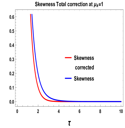
Refer to caption
(a) Skewness for lower values μkτsubscript𝜇𝑘𝜏\mu_{k}\tau
Refer to caption
(b) Skewness for all values μkτsubscript𝜇𝑘𝜏\mu_{k}\tau
Figure 53: Time dependent behaviour of Skewness without correction and with correction at different fixed range of μksubscript𝜇𝑘\mu_{k}.

Now from fig. 53, we can say that the corrected Skewness deviate significantly from the uncorrected one at low μkτsubscript𝜇𝑘𝜏\mu_{k}\tau limit. But we can see that at higher limit they overlap. Also Skewness is positive for the whole range which implies that the normal distribution curve has longer right tail. Moreover, there is a discontinuity of third order corrected Skewness in between the range 0.1<τ<10.1𝜏10.1<\tau<1 and for the rest of the whole range of time Skewness decreased upto unity and then it is increased.

6.4.3 Kurtosis

Kurtosis is a measure of the tailedness of the probability distribution of a real-valued random variable. This is actually a descriptor of the shape of a probability distribution function and there are specific ways of quantifying it for a theoretical probability distribution and corresponding ways of estimating it from a sample from a population. It is important to note that, the Kurtosis of any univariate normal distribution is 333. For practical purposes it is common practice to compare the expression for Kurtosis of a probability distribution function to 333. Probability distributions with Kurtosis less than the value 333 are identified as platykurtic, although this information does not imply the distribution is flat-topped in nature. Rather, it implies that the probability distribution produces fewer and less extreme outliers than does the normal probability distribution. Probability distributions with Kurtosis greater than the value 333 are said to be leptokurtic. It is also common practice to use, the excess Kurtosis, which is the Kurtosis minus 333, to provide the comparison to the normal probability distribution profile. Like Skewness here also we calculate kurtosis from different distribution and get it at different order of correction.

Therefore, Kurtosis without correction can be expressed as:

𝐊𝐮𝐫𝐭𝐨𝐬𝐢𝐬𝐮𝐜subscript𝐊𝐮𝐫𝐭𝐨𝐬𝐢𝐬𝐮𝐜\displaystyle{\bf Kurtosis_{uc}} =\displaystyle= n4𝐈[n2𝐈(n𝐈)2]2subscriptdelimited-⟨⟩superscript𝑛4𝐈superscriptdelimited-[]subscriptdelimited-⟨⟩superscript𝑛2𝐈superscriptsubscriptdelimited-⟨⟩𝑛𝐈22\displaystyle\frac{\langle n^{4}\rangle_{{\color[rgb]{1,0,0}\bf I}}}{\left[\langle n^{2}\rangle_{{\color[rgb]{1,0,0}\bf I}}-\left(\langle n\rangle_{{\color[rgb]{1,0,0}\bf I}}\right)^{2}\right]^{2}} (807)
=\displaystyle= n4𝐈[𝐒.𝐃.𝐮𝐜]2\displaystyle\frac{\langle n^{4}\rangle_{{\color[rgb]{1,0,0}\bf I}}}{\left[{\bf S.D._{uc}}\right]^{2}}
=\displaystyle= 6μ(3e4μkτ+2e6μkτ+1)6𝜇3superscript𝑒4subscript𝜇𝑘𝜏2superscript𝑒6subscript𝜇𝑘𝜏1\displaystyle\frac{6}{\mu\left(-3e^{4\mu_{k}\tau}+2e^{6\mu_{k}\tau}+1\right)}
×[6(μk1)e2μkτ+3(5μk2)e8μkτ\displaystyle~{}\times\left[6(\mu_{k}-1)e^{2\mu_{k}\tau}+3(5\mu_{k}-2)e^{8\mu_{k}\tau}\right.
2e6μkτ(3μ(4μkτ+3)5)3μk+2].\displaystyle\left.~{}~{}~{}~{}~{}~{}~{}~{}~{}~{}~{}~{}~{}~{}-2e^{6\mu_{k}\tau}(3\mu(4\mu_{k}\tau+3)-5)-3\mu_{k}+2\right].

On the other hand, the fourth order corrected value of the Kurtosis can be expressed as:

𝐊𝐮𝐫𝐭𝐨𝐬𝐢𝐬𝐜subscript𝐊𝐮𝐫𝐭𝐨𝐬𝐢𝐬𝐜\displaystyle{\bf Kurtosis_{c}} =\displaystyle= n4𝐈+n4𝐈𝐈+n4𝐈𝐈𝐈+n4𝐈𝐕[n2𝐈+n2𝐈(n𝐈)2]2subscriptdelimited-⟨⟩superscript𝑛4𝐈subscriptdelimited-⟨⟩superscript𝑛4𝐈𝐈subscriptdelimited-⟨⟩superscript𝑛4𝐈𝐈𝐈subscriptdelimited-⟨⟩superscript𝑛4𝐈𝐕superscriptdelimited-[]subscriptdelimited-⟨⟩superscript𝑛2𝐈subscriptdelimited-⟨⟩superscript𝑛2𝐈superscriptsubscriptdelimited-⟨⟩𝑛𝐈22\displaystyle\frac{\langle n^{4}\rangle_{{\color[rgb]{1,0,0}\bf I}}+\langle n^{4}\rangle_{{\color[rgb]{1,0,0}\bf II}}+\langle n^{4}\rangle_{{\color[rgb]{1,0,0}\bf III}}+\langle n^{4}\rangle_{{\color[rgb]{1,0,0}\bf IV}}}{\left[\langle n^{2}\rangle_{{\color[rgb]{1,0,0}\bf I}}+\langle n^{2}\rangle_{{\color[rgb]{1,0,0}\bf I}}-\left(\langle n\rangle_{{\color[rgb]{1,0,0}\bf I}}\right)^{2}\right]^{2}} (808)
=\displaystyle= n4𝐈+n4𝐈𝐈+n4𝐈𝐈𝐈+n4𝐈𝐕[𝐒.𝐃.c]2\displaystyle\frac{\langle n^{4}\rangle_{{\color[rgb]{1,0,0}\bf I}}+\langle n^{4}\rangle_{{\color[rgb]{1,0,0}\bf II}}+\langle n^{4}\rangle_{{\color[rgb]{1,0,0}\bf III}}+\langle n^{4}\rangle_{{\color[rgb]{1,0,0}\bf IV}}}{\left[{\bf S.D.}_{c}\right]^{2}}
Refer to caption
(a) Corrected Kurtosis for large values μkτsubscript𝜇𝑘𝜏\mu_{k}\tau
Refer to caption
(b) Corrected Kurtosis for small values τ𝜏\tau
Figure 54: Time dependent behaviour of Kurtosis without correction and with correction in the probability density distribution function at different range of τ𝜏\tau considering different μksubscript𝜇𝑘\mu_{k}

From fig. (54), we can say that uncorrected kurtosis deviate from corrected one in lower τ𝜏\tau regime though overlapped in higher order [τ>1𝜏1\tau>1]. So the contribution from the correction factor is important in lower regime. Also it is important to note that, Kurtosis is greater than the value 333 for the whole time regime, so the distribution is Leptokurtic and have fatter tails.Here fig 54(a) has a huge value for corrected kurtosis which can be bounded within a particular value using tuning parameter.

From the calculation of the higher-order statistical moments (or equivalently the amplitude of the quantum mechanical correlation functions) we get the following overall features to analyze the nature and physical outcomes of the corrected probability density function derived in this paper.

  1. 1.

    The Standard Deviation is significantly large for higher μkτsubscript𝜇𝑘𝜏\mu_{k}\tau, though very small for lower regime.

  2. 2.

    Skewness is positive throughout the time regime, though becomes vanishingly small at a specific time interval (0.1<τ<0.70.1𝜏0.70.1<\tau<0.7).

  3. 3.

    Kurtosis is greater than 333 for the whole time regime.

  4. 4.

    The predicted Log-Normal Gaussian Distribution shows deviations at significant levels. Effects of the non-Gaussianity in the distribution function is clearly visualized.

  5. 5.

    The probability distribution has longer trailing ends and the trails go broad higher.

  6. 6.

    The probability distribution has a very low spread at lower μkτsubscript𝜇𝑘𝜏\mu_{k}\tau limit though highly spread out in larger limit.

Conequently, from the previously predicted result of Amin:2015ftc we show that distribution deviates from a Log-Normal distribution and the predicted distribution function appears to be leptokurtic and has a broad right trailing end.All of this portion have a simmilar connection with ref  Choudhury:2018bcf

7 Conclusion

In this paper we have addressed the issues which are appended below:

  • In this paper, we have provided the analogy between particle creation in primordial cosmology and scattering problem inside a conduction wire in presence of impurities. Such impurities are characterized by effective potential in the context of quantum mechanical description. On the other hand, in the context of primordial cosmology time dependent mass profile of created particles (couplings) mimics the same role.

  • Specific time dependence of mass profile actually restricts the structure of the scattering effective potential. To establish the analogy between two theoretical frameworks we have further computed various characteristic features of conduction wire i.e. resistance, conductance (electrical properties), Lyapunov exponent (dynamical property), reflection and transmission coefficients (optical properties), occupation number and energy density (energetics) using the expression for Bogoliubov coefficients for different mass profiles which connects the ingoing and outgoing solution of the mode functions obtained in the context of particle creation process in cosmology.

  • We have solved this particle creation problem using the following crucial steps:

    1. 1.

      First of all assuming that the interactions are well known we have studied the one to one correspondence between the particle creation problem in early universe cosmology with the scattering problem inside a conduction wire. Here we have additionally neglected the effect of the expansion of our universe and this is perfectly justifiable during the epoch of reheating. For this reason we call it as Reheating Approximation.

    2. 2.

      Secondly we have studied the same problem where the particle interactions are not known at all at the level of action. In such a situation, assuming the gravitational background is classical in nature and also assuming the previously mentioned Reheating Approximation we have demonstrated the problem with the help of Random Matrix Theory.

    3. 3.

      Further we have solved the dynamics of the particle creation problem by studying the higher order corrections in the Fokker Planck equation for previously mentioned random system where the interactions are not easily quantifiable at the level of action. We have constructed the fourth order corrected Fokker Planck equation from which we have provided the solution of the random probability distribution function. Such distributions are very very useful to study the dynamical systems when particle interactions are not well known. In our analysis we have identified all of these modifications as the quantum correction to the Fokker-Planck equation, the physical implications of which we have studied in detail in this paper.

  • In this work, we have shown that the Lyapunov exponent varies inversely with the number of scatterers. Therefore, with an increase in the number of scatterers the Lyapunov exponent also reduces thereby reducing the amount of randomness in the system. This may be a hint to the fact that the Lyapunov exponent has a dependence on the momenta values of the incoming wave-function of the scalar field. Additionally, it is important to note that the upper bound of Lyuapunov exponent is restricted by the constraint λ2π/β𝜆2𝜋𝛽\lambda\leq 2\pi/\beta (where β=1/T𝛽1𝑇\beta=1/T), which is a generic bound on chaos obtained in the context of quantum field theory. As a consequence, one can find restriction on the upper bound on the reheating temperature for the different quenched mass profiles for which the chaos bound saturates. This is obviously a remarkable result in the present context as it can able to provide the explicit expression for the reheating temperature for a specified momentum scale, which was not predicted earlier in the detailed study of reheating. Most importantly, the bound on quantum chaos in terms of Lyapunov exponent directly restrict the value of reheating temperature without explicitly knowing the details of the particle interactions as appearing in the action. Just the knowledge of time dependence of the quenched mass profiles (in other words the knowledge of effective impurity potential as appearing inside the conduction wire) is sufficient enough to restrict the upper bound of reheating temperature due to quantum chaos.

  • In this context we have also provided the expression for the two point quantum correlation function, which is known as Spectral Form Factor (SFF) for both in finite and zero temperature. Spectral Form Factor is actually a more strong measure to find chaotic behaviour of a dynamical system compared to Lyapunov exponent. We get saturating behaviour of SFF at late time scale, which indicates that it has an upper-bound. We can relate SFF for any potential (Even Polynomial Potential in this case). In the calculation of the Lyapunov Exponent for the specific time dependent mass profiles, we choose three different quenched protocols for mass profiles. Potential functions which can be represented by polynomial potential (Even only in our case) can be used to get the SFF-saturation. In this connection ,we have provided a model independent upper and lower bound of SFF, which is treated as the significant bound of quantum chaos (1/N(11/π)𝐒𝐅𝐅1/πN1𝑁11𝜋𝐒𝐅𝐅1𝜋𝑁-1/N\left(1-1/\pi\right)\leq{\bf SFF}\leq 1/\pi N) in the context of particle production event in cosmology. This is obviously a remarkable result which we have explicitly computed in this paper.In Choudhury:2018lcb this same has been calculated for general polynomial with GUE.

  • We have also presented the computation of quantum corrected Fokker- Planck equation which corresponds to the delta-scatterers. From this computation we have derived the corrected statistical distribution of the particle production events in cosmology. The distribution which has been predicted in Amin:2015ftc to be Gaussian doesn’t retain its form when more correction terms are taken into account. This may be treated as a signature of non-Gaussian in particle production events during reheating (in cosmology).

The future discussions of the present work are mentioned in the following:

  • In this paper for our study of quantum chaos in the context of cosmology we have used a closed quantum system. As we have mentioned that the present computation has been performed for a massless scalar field which interacts with the heavy fields (which acts like scatterers inside the conduction wire). The entire calculation is being done for the set up when there is only a single massless scalar field that interacts with the scatterer. One may repeat the calculation for a large number of these scalar fields interacting with the scatterers which needs the introduction of the random matrix approach in a more generalized fashion.

  • The system we have studied in this paper have no interactions with the background as the definition of the background in this set-up is itself an ill-defined one during reheating. To treat the entire system having being interacted with a background one needs to have a detailed description of the nature of background in the cosmological scenario. Then it will be possible to introduce the other non-linear and dissipative effects into the system introduced by the background itself. Such a treatment will be studied within the framework of an open quantum system interacting with the defined background set-up. One then needs to consider the entire system having being interacted with the background under a weak coupling limit. One such model as has been studied in Shandera:2017qkg .

  • We have calculated the Lyapunov exponent and Spectral Form Factor in this paper which is a measure of chaos or non-linearity into the system. With the system prescribed in this work being treated as an open quantum system one may study the effects of dissipation being introduced into such a system which renders the system to be a stochastic one. With this, one may be able to study the effects of the non-linearity being introduced into the system which may well be a good study to look for the behaviour of Lyapunov exponent and Spectral Form Factor.

  • During the study of quantum correction in the Fokker Planck equation and the deviation from log normal distribution we have followed a specific approach in which we have considered the following possibilities:

    1. 1.

      We have neglected the contribution from the damping term in the Fokker Planck equation. One can include such effect and study its role in the context of cosmology (specifically during reheating).

    2. 2.

      During the computation we have followed a specific approach in which we have also neglected the effect of impurity potential at very high temperature during reheating. This will give rise to a simplest form of the Fokker Planck equation where only diffusion and drift contributions are appearing explicitly. But if we include the effect of impurity potential in presence of finite temperature then it will surely effect the final solution of the probability distribution function. One can include such additional effects and study its impact during reheating epoch of the early universe.

    3. 3.

      Furthermore, during the construction of the Fokker Planck equation from the basic principles we have followed a special approach in which the effect of diffusion and drift is appearing in a very simplified manner. However, in the study of statistical field theory Ito^^𝑜\hat{o} and Stratnovitch or more generalized prescriptions are used commonly to construct the Fokker Planck equation. Here it is important to note that in each case it will give rise to different mathematical structure of Fokker Planck equations. In the present context of discussion, one can follow such well known prescriptions to see its physical outcomes to solve the probability distribution function for the particle production and compare the results to check the appropriateness of these approaches during reheating.

Acknowledgments

SC would like to thank Quantum Gravity and Unified Theory and Theoretical Cosmology Group, Max Planck Institute for Gravitational Physics, Albert Einstein Institute for providing the Post-Doctoral Research Fellowship. SC would like to thank IUCAA, Pune, India where the problem was formulated and part of the work has been done during post doctoral tenure. SC take this opportunity to thank sincerely to Jean-Luc Lehners, Shiraz Minwalla, Sudhakar Panda and Varun Sahni for their constant support and inspiration. SC thank the organisers of Summer School on Cosmology 2018, ICTP, Trieste, 15 th Marcel Grossman Meeting, Rome, The European Einstein Toolkit meeting 2018, Centra, Instituto Superior Tecnico, Lisbon, The Universe as a Quantum Lab, APC, Paris, LMU Quantum Gravity School, Munich, Nordic String Meeting 2019, AEI, Summer meeting on String Cosmology, DESY, Zeuthen, Kavli Asian WInter School on Strings, Particles and Cosmology 2018 for providing the local hospitality during the work. SC also thank DTP, TIFR, Mumbai, ICTS, TIFR, Bengaluru, IOP, Bhubaneswar, CMI, Chennai, SINP, Kolkata and IACS, Kolkata for providing the academic visit during the work. AM, PC and SB are thankful to IUCAA, Pune for the visit during the work for winter project. Last but not the least, We would all like to acknowledge our debt to the people of India for their generous and steady support for research in natural sciences, especially for theoretical high energy physics, string theory and cosmology.

Appendix A Ito^^𝑜\hat{o} solution of Fokker Planck equation

Refer to caption
Figure 55: Evolution of the probability density function for Ito^^𝑜\hat{o} prescription with respect to the the occupation number per mode n𝑛n, for a fixed time.

From Ito^^𝑜\hat{o} perspective the Fokker Planck equation can be expressed as:

𝐅𝐨𝐤𝐤𝐞𝐫𝐏𝐥𝐚𝐧𝐜𝐤𝐄𝐪𝐮𝐚𝐭𝐢𝐨𝐧(𝐅𝐫𝐨𝐦𝐈𝐭𝐨^)¯::¯𝐅𝐨𝐤𝐤𝐞𝐫𝐏𝐥𝐚𝐧𝐜𝐤𝐄𝐪𝐮𝐚𝐭𝐢𝐨𝐧𝐅𝐫𝐨𝐦𝐈𝐭^𝐨absent\displaystyle{\color[rgb]{0,0,1}\bf\underline{Fokker~{}Planck~{}Equation~{}(From~{}It\hat{o})}:}
P(n;τ)τ𝑃𝑛𝜏𝜏\displaystyle\frac{\partial P(n;\tau)}{\partial\tau} =\displaystyle= n(a(n)P(n;τ))+2n2(D(n)P(n;τ)),𝑛𝑎𝑛𝑃𝑛𝜏superscript2superscript𝑛2𝐷𝑛𝑃𝑛𝜏\displaystyle-\frac{\partial}{\partial n}\left(a(n)P(n;\tau)\right)+\frac{\partial^{2}}{\partial n^{2}}\left(D(n)P(n;\tau)\right), (809)

Here we take a(n)=0𝑎𝑛0a(n)=0 and D(n)=n(n+1)𝐷𝑛𝑛𝑛1D(n)=n(n+1). Using this we get the following solution of probability distribution:

P(n,τ)𝑃𝑛𝜏\displaystyle P(n,\tau) =\displaystyle= 12πn(n+1)τμkexp[((4n+2)τμk+n)24n(n+1)τμk]\displaystyle\frac{1}{2\sqrt{\pi}\sqrt{n(n+1)\tau\mu_{k}}}\exp\left[-\frac{((4n+2)\tau\mu_{k}+n){}^{2}}{4n(n+1)\tau\mu_{k}}\right] (810)

In fig. (55) we have shown the probability distribution function obtained from the Ito^^𝑜\hat{o} solution of the Fokker Planck equation. This solution is similar to the log normal distribution obtained from the present computation. From the plot we observe that for large value of occupation number n𝑛n (n>>1much-greater-than𝑛1n>>1) the distribution function decays to a finite saturation value. On the other hand for small occupation number n𝑛n (n<<1much-less-than𝑛1n<<1) we get peak in the distribution function for different values of μkτsubscript𝜇𝑘𝜏\mu_{k}\tau.

Appendix B Stratonovitch solution of Fokker Planck equation
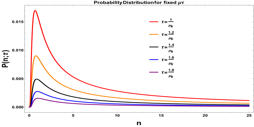
Refer to caption
Figure 56: Evolution of the probability density function for Stratonovitch prescription with respect to the the occupation number per mode n𝑛n, for a fixed time in the limit n<<1much-less-than𝑛1n<<1.

From Stratonovitch perspective the Fokker Planck equation can be expressed as:

𝐅𝐨𝐤𝐤𝐞𝐫𝐏𝐥𝐚𝐧𝐜𝐤𝐄𝐪𝐮𝐚𝐭𝐢𝐨𝐧(𝐅𝐫𝐨𝐦𝐒𝐭𝐫𝐚𝐭𝐨𝐧𝐨𝐯𝐢𝐭𝐜𝐡)¯::¯𝐅𝐨𝐤𝐤𝐞𝐫𝐏𝐥𝐚𝐧𝐜𝐤𝐄𝐪𝐮𝐚𝐭𝐢𝐨𝐧𝐅𝐫𝐨𝐦𝐒𝐭𝐫𝐚𝐭𝐨𝐧𝐨𝐯𝐢𝐭𝐜𝐡absent\displaystyle{\color[rgb]{0,0,1}\bf\underline{Fokker~{}Planck~{}Equation~{}(From~{}Stratonovitch)}:}
P(n;τ)τ𝑃𝑛𝜏𝜏\displaystyle\frac{\partial P(n;\tau)}{\partial\tau} =\displaystyle= n(a(n)P(n;τ))+n(D(n)n(D(n)P(n;τ))),𝑛𝑎𝑛𝑃𝑛𝜏𝑛𝐷𝑛𝑛𝐷𝑛𝑃𝑛𝜏\displaystyle-\frac{\partial}{\partial n}\left(a(n)P(n;\tau)\right)+\frac{\partial}{\partial n}\left(\sqrt{D(n)}\frac{\partial}{\partial n}\left(\sqrt{D(n)}P(n;\tau)\right)\right), (811)

Here we take a(n)=0𝑎𝑛0a(n)=0 and D(n)=n(n+1)𝐷𝑛𝑛𝑛1D(n)=n(n+1). Using this we get the following solution of probability distribution:

P(n,τ)𝑃𝑛𝜏\displaystyle P(n,\tau) =\displaystyle= 12πn(n+1)τμkexp[9(2n+1)2τμk16n(n+1)]12𝜋𝑛𝑛1𝜏subscript𝜇𝑘9superscript2𝑛12𝜏subscript𝜇𝑘16𝑛𝑛1\displaystyle\frac{1}{2\sqrt{\pi}\sqrt{n(n+1)\tau\mu_{k}}}\exp\left[-\frac{9(2n+1)^{2}\tau\mu_{k}}{16n(n+1)}\right] (812)

In fig. (56) we have shown the probability distribution function obtained from the Stratonovitch solution of the Fokker Planck equation. This solution is similar to the log normal distribution obtained from the present computation. From the plot we observe that for large value of occupation number n𝑛n (n>>1much-greater-than𝑛1n>>1) the distribution function decays to a finite saturation value. On the other hand for small occupation number n𝑛n (n<<1much-less-than𝑛1n<<1) we get peak in the distribution function for different values of μkτsubscript𝜇𝑘𝜏\mu_{k}\tau.

Appendix C Generalized solution of Fokker Planck equation at infinite temperature
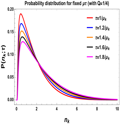
Refer to caption
(a) Probability distribution for Q=1/4𝑄14Q=1/4.
Refer to caption
(b) Probability distribution for Q=1/8𝑄18Q=1/8.
Figure 57: Evolution of the probability density function for generalized prescription with respect to the the occupation number per mode n𝑛n, for a fixed time.

From General perspective the Fokker Planck equation can be expressed as:

𝐅𝐨𝐤𝐤𝐞𝐫𝐏𝐥𝐚𝐧𝐜𝐤𝐄𝐪𝐮𝐚𝐭𝐢𝐨𝐧(𝐅𝐨𝐫𝐆𝐞𝐧𝐞𝐫𝐚𝐥𝐢𝐳𝐞𝐝𝐈𝐭𝐨^)¯::¯𝐅𝐨𝐤𝐤𝐞𝐫𝐏𝐥𝐚𝐧𝐜𝐤𝐄𝐪𝐮𝐚𝐭𝐢𝐨𝐧𝐅𝐨𝐫𝐆𝐞𝐧𝐞𝐫𝐚𝐥𝐢𝐳𝐞𝐝𝐈𝐭^𝐨absent\displaystyle{\color[rgb]{0,0,1}\bf\underline{Fokker~{}Planck~{}Equation~{}(For~{}Generalized~{}It\hat{o})}:}
P(n;τ)τ𝑃𝑛𝜏𝜏\displaystyle\frac{\partial P(n;\tau)}{\partial\tau} =\displaystyle= n(a(n)P(n;τ))+n((D(n))1Qn((D(n))QP(n;τ))),𝑛𝑎𝑛𝑃𝑛𝜏𝑛superscript𝐷𝑛1𝑄𝑛superscript𝐷𝑛𝑄𝑃𝑛𝜏\displaystyle-\frac{\partial}{\partial n}\left(a(n)P(n;\tau)\right)+\frac{\partial}{\partial n}\left((D(n))^{1-Q}\frac{\partial}{\partial n}\left((D(n))^{Q}P(n;\tau)\right)\right),~{}~{}~{}~{}~{}~{} (813)

Here we take a(n)=0𝑎𝑛0a(n)=0 and D(n)=n(n+1)𝐷𝑛𝑛𝑛1D(n)=n(n+1). Using this we get the following solution of probability distribution:

P(n,τ)𝑃𝑛𝜏\displaystyle P(n,\tau) =\displaystyle= 12μkπτ(n(n+1))Q12subscript𝜇𝑘𝜋𝜏superscript𝑛𝑛1𝑄\displaystyle\frac{1}{2\sqrt{\mu_{k}\pi\tau(n(n+1))^{Q}}} (814)
×exp[(n2(n+1)+μkτ(2n+1)Q(Q+1)(n(n+1))Q)24μkτ(n(n+1))Q+2]absentsuperscriptsuperscript𝑛2𝑛1subscript𝜇𝑘𝜏2𝑛1𝑄𝑄1superscript𝑛𝑛1𝑄24subscript𝜇𝑘𝜏superscript𝑛𝑛1𝑄2\displaystyle~{}~{}~{}~{}~{}~{}~{}~{}~{}\times\exp\left[-\frac{\left(n^{2}(n+1)+\mu_{k}\tau(2n+1)Q(Q+1)(n(n+1))^{Q}\right)^{2}}{4\mu_{k}\tau(n(n+1))^{Q+2}}\right]~{}~{}~{}~{}~{}~{}

In fig. (57) we have shown the probability distribution function obtained from the generalized solution of the Fokker Planck equation without dissipation in very very large temperature. From the plot we observe that for large value of occupation number n𝑛n (n>>1much-greater-than𝑛1n>>1) the distribution function decays to a finite saturation value. On the other hand for small occupation number n𝑛n (n<<1much-less-than𝑛1n<<1) we get peak in the distribution function for different values of μkτsubscript𝜇𝑘𝜏\mu_{k}\tau.

Appendix D Generalized solution of Fokker Planck equation at finite temperature

From General perspective the Fokker Planck equation with effect of potential can be expressed as:

𝐄𝐟𝐟𝐞𝐜𝐭𝐢𝐯𝐞𝐏𝐨𝐭𝐞𝐧𝐭𝐢𝐚𝐥:¯¯:𝐄𝐟𝐟𝐞𝐜𝐭𝐢𝐯𝐞𝐏𝐨𝐭𝐞𝐧𝐭𝐢𝐚𝐥absent\displaystyle{\color[rgb]{0,0,1}\bf\underline{Effective~{}Potential:}}
U(n)𝑈𝑛\displaystyle U(n) =\displaystyle= [β24D(n)(V(n)n)2β2D(n)(2V(n)n2)β2(D(n)n)(V(n)n)].delimited-[]superscript𝛽24𝐷𝑛superscript𝑉𝑛𝑛2𝛽2𝐷𝑛superscript2𝑉𝑛superscript𝑛2𝛽2𝐷𝑛𝑛𝑉𝑛𝑛\displaystyle\left[\frac{\beta^{2}}{4}D(n)\left(\frac{\partial V(n)}{\partial n}\right)^{2}-\frac{\beta}{2}D(n)\left(\frac{\partial^{2}V(n)}{\partial n^{2}}\right)-\frac{\beta}{2}\left(\frac{\partial D(n)}{\partial n}\right)\left(\frac{\partial V(n)}{\partial n}\right)\right]. (815)
n(D(n)W(n;τ)n)U(n)W(n;τ)𝑛𝐷𝑛𝑊𝑛𝜏𝑛𝑈𝑛𝑊𝑛𝜏\displaystyle\frac{\partial}{\partial n}\left(D(n)\frac{\partial W(n;\tau)}{\partial n}\right)-U(n)W(n;\tau) =\displaystyle= W(n;τ)τ,𝑊𝑛𝜏𝜏\displaystyle\frac{\partial W(n;\tau)}{\partial\tau}, (816)
P(n;τ)𝑃𝑛𝜏\displaystyle P(n;\tau) =\displaystyle= exp(β2V(n))W(n;τ).𝛽2𝑉𝑛𝑊𝑛𝜏\displaystyle\exp\left(-\frac{\beta}{2}V(n)\right)W(n;\tau)~{}. (817)

Here we take a(n)=0𝑎𝑛0a(n)=0,V[n]=n2𝑉delimited-[]𝑛superscript𝑛2V[n]=n^{2}and D(n)=n(n+1)𝐷𝑛𝑛𝑛1D(n)=n(n+1). Using this we get the following solution of probability distribution:

P(n,τ)𝑃𝑛𝜏\displaystyle~{}P(n,\tau) =\displaystyle= 12πn(n+1)τμk12𝜋𝑛𝑛1𝜏subscript𝜇𝑘\displaystyle\frac{1}{2\sqrt{\pi}\sqrt{n(n+1)\tau\mu_{k}}} (818)
×exp[(nμk(2nτ+τ))24n(n+1)τμkβn22βn{n(βn(n+1)3)2}]\displaystyle~{}~{}~{}\times\exp\left[-\frac{(n-\mu_{k}(2n\tau+\tau)){}^{2}}{4n(n+1)\tau\mu_{k}}-\frac{\beta n^{2}}{2}-\beta n\left\{n(\beta n(n+1)-3)-2\right\}\right]~{}~{}~{}~{}
Refer to caption
(a) Probability distribution for β=0.01𝛽0.01\beta=0.01.
Refer to caption
(b) Probability distribution for β=1𝛽1\beta=1.
Refer to caption
(c) Probability distribution for β=10𝛽10\beta=10.
Refer to caption
(d) Probability distribution for β=100𝛽100\beta=100.
Figure 58: Evolution of the probability density function for generalized prescription with respect to the the occupation number per mode n𝑛n, for a fixed time and β𝛽\beta.

In fig. (58) we have shown the probability distribution function obtained from the solution of of the Fokker Planck equation derived in presence of finite temperature effective potential solution. From the plot we observe that for large value of occupation number n𝑛n (n>>1much-greater-than𝑛1n>>1) the distribution function decays to a finite saturation value. On the other hand for small occupation number n𝑛n (n<<1much-less-than𝑛1n<<1) we get peak in the distribution function for different values of μkτsubscript𝜇𝑘𝜏\mu_{k}\tau.

References

  • (1) D. Baumann, ”Inflation” doi:10.1142/97898143271830010,arXiv:0907.5424[hepth]:𝑑𝑜𝑖10.1142subscript97898143271830010𝑎𝑟𝑋𝑖𝑣:0907.5424delimited-[]𝑒𝑝𝑡doi:10.1142/9789814327183_{0}010,arXiv:0907.5424[hep-th]
  • (2) D. Baumann, “TASI Lectures on Primordial Cosmology” arXiv:1807.03098 [hep-th].
  • (3) D. Baumann and L. McAllister, “Inflation and String Theory,” doi:10.1017/CBO9781316105733 arXiv:1404.2601 [hep-th]
  • (4) C. Cheung, P. Creminelli, A. L. Fitzpatrick, J. Kaplan and L. Senatore, “The Effective Field Theory of Inflation,” JHEP 0803 (2008) 014 doi:10.1088/1126-6708/2008/03/014 [arXiv:0709.0293 [hep-th]].
  • (5) S. Weinberg, “Effective Field Theory for Inflation,” Phys. Rev. D 77 (2008) 123541 doi:10.1103/PhysRevD.77.123541 [arXiv:0804.4291 [hep-th]].
  • (6) L. V. Delacretaz, V. Gorbenko and L. Senatore, “The Supersymmetric Effective Field Theory of Inflation,” JHEP 1703 (2017) 063 doi:10.1007/JHEP03(2017)063 [arXiv:1610.04227 [hep-th]].
  • (7) L. Senatore, “Lectures on Inflation,” doi:10.1142/9789813149441-0008, arXiv:1609.00716 [hep-th].
  • (8) L. V. Delacretaz, T. Noumi and L. Senatore, “Boost Breaking in the EFT of Inflation,” JCAP 1702 (2017) no.02, 034 doi:10.1088/1475-7516/2017/02/034 [arXiv:1512.04100 [hep-th]].
  • (9) D. Lopez Nacir, R. A. Porto, L. Senatore and M. Zaldarriaga, “Dissipative effects in the Effective Field Theory of Inflation,” JHEP 1201 (2012) 075 doi:10.1007/JHEP01(2012)075 [arXiv:1109.4192 [hep-th]].
  • (10) L. Senatore and M. Zaldarriaga, “The Effective Field Theory of Multifield Inflation,” JHEP 1204 (2012) 024 doi:10.1007/JHEP04(2012)024 [arXiv:1009.2093 [hep-th]].
  • (11) S. Choudhury and S. Pal, “Brane inflation in background supergravity,” Phys. Rev. D 85 (2012) 043529 doi:10.1103/PhysRevD.85.043529 [arXiv:1102.4206 [hep-th]].
  • (12) S. Choudhury and S. Pal, “Fourth level MSSM inflation from new flat directions,” JCAP 1204, 018 (2012) doi:10.1088/1475-7516/2012/04/018 [arXiv:1111.3441 [hep-ph]].
  • (13) S. Choudhury and S. Pal, “DBI Galileon inflation in background SUGRA,” Nucl. Phys. B 874 (2013) 85 doi:10.1016/j.nuclphysb.2013.05.010 [arXiv:1208.4433 [hep-th]].
  • (14) S. Choudhury, T. Chakraborty and S. Pal, “Higgs inflation from new Kähler potential,” Nucl. Phys. B 880 (2014) 155 doi:10.1016/j.nuclphysb.2014.01.002 [arXiv:1305.0981 [hep-th]].
  • (15) S. Choudhury, A. Mazumdar and S. Pal, “Low and High scale MSSM inflation, gravitational waves and constraints from Planck,” JCAP 1307 (2013) 041 doi:10.1088/1475-7516/2013/07/041 [arXiv:1305.6398 [hep-ph]].
  • (16) S. Choudhury and A. Mazumdar, “An accurate bound on tensor-to-scalar ratio and the scale of inflation,” Nucl. Phys. B 882 (2014) 386 doi:10.1016/j.nuclphysb.2014.03.005 [arXiv:1306.4496 [hep-ph]].
  • (17) S. Choudhury, A. Mazumdar and E. Pukartas, “Constraining 𝒩=1𝒩1{\cal N}=1 supergravity inflationary framework with non-minimal Kähler operators,” JHEP 1404 (2014) 077 doi:10.1007/JHEP04(2014)077 [arXiv:1402.1227 [hep-th]].
  • (18) S. Choudhury and A. Mazumdar, “Reconstructing inflationary potential from BICEP2 and running of tensor modes, arXiv:1403.5549 [hep-th].
  • (19) S. Choudhury, “Can Effective Field Theory of inflation generate large tensor-to-scalar ratio within Randall–Sundrum single braneworld?,” Nucl. Phys. B 894 (2015) 29 doi:10.1016/j.nuclphysb.2015.02.024 [arXiv:1406.7618 [hep-th]].
  • (20) S. Choudhury, B. K. Pal, B. Basu and P. Bandyopadhyay, “Quantum Gravity Effect in Torsion Driven Inflation and CP violation,” JHEP 1510 (2015) 194 doi:10.1007/JHEP10(2015)194 [arXiv:1409.6036 [hep-th]].
  • (21) S. Choudhury and S. Panda, “COSMOS-e’-GTachyon from string theory” Eur. Phys. J. C 76 (2016) no.5, 278 doi:10.1140/epjc/s10052-016-4072-2 [arXiv:1511.05734 [hep-th]].
  • (22) S. Choudhury, “COSMOS-esuperscript𝑒e^{\prime}- soft Higgsotic attractors,” Eur. Phys. J. C 77 (2017) no.7, 469 doi:10.1140/epjc/s10052-017-5001-8 [arXiv:1703.01750 [hep-th]].
  • (23) A. Naskar, S. Choudhury, A. Banerjee and S. Pal, “Inflation to Structures: EFT all the way, arXiv:1706.08051 [astro-ph.CO].
  • (24) S. Choudhury, “CMB from EFT” arXiv:1712.04766 [hep-th].
  • (25) S. Choudhury, “Reconstructing inflationary paradigm within Effective Field Theory framework” Phys. Dark Univ.  11 (2016) 16 doi:10.1016/j.dark.2015.11.003 [arXiv:1508.00269 [astro-ph.CO]].
  • (26) S. Choudhury and S. Pal, “Reheating and leptogenesis in a SUGRA inspired brane inflation” Nucl. Phys. B 857 (2012) 85 doi:10.1016/j.nuclphysb.2011.12.006 [arXiv:1108.5676 [hep-ph]].
  • (27) L. Kofman, A. D. Linde and A. A. Starobinsky, “Reheating after inflation” Phys. Rev. Lett.  73 (1994) 3195 doi:10.1103/PhysRevLett.73.3195 [hep-th/9405187].
  • (28) Y. Shtanov, J. H. Traschen and R. H. Brandenberger, “Universe reheating after inflation” Phys. Rev. D 51 (1995) 5438 doi:10.1103/PhysRevD.51.5438 [hep-ph/9407247].
  • (29) M. A. Amin, M. P. Hertzberg, D. I. Kaiser and J. Karouby, “Nonperturbative Dynamics Of Reheating After Inflation: A Review”, Int. J. Mod. Phys. D 24 (2014) 1530003 doi:10.1142/S0218271815300037 [arXiv:1410.3808 [hep-ph]].
  • (30) O. Özsoy, G. Sengor, K. Sinha and S. Watson, “A Model Independent Approach to (p)Reheating” arXiv:1507.06651 [hep-th].
  • (31) O. Özsoy, J. T. Giblin, E. Nesbit, G. Şengör and S. Watson, “Toward an Effective Field Theory Approach to Reheating’ Phys. Rev. D 96 (2017) no.12, 123524 doi:10.1103/PhysRevD.96.123524 [arXiv:1701.01455 [hep-th]].
  • (32) L. Kofman and P. Yi, “Reheating the universe after string theory inflation’ Phys. Rev. D 72 (2005) 106001 doi:10.1103/PhysRevD.72.106001 [hep-th/0507257].
  • (33) G. W. Gibbons and S. W. Hawking, ”Cosmological Event Horizons, Thermodynamics, and Particle Creation”, Phys. Rev. D 15, 2738 (1977)
  • (34) R. Schutzhold and W. G. Unruh, ”Cosmological particle creation in the lab?”, Lect. Notes Phys.  870, 51 (2013) [arXiv:1203.1173 [gr-qc]]
  • (35) S. Winitzki, ”Cosmological particle production and the precision of the WKB approximation”, Phys. Rev. D 72, 104011 (2005) /PhysRevD.72.104011 [gr-qc/0510001].
  • (36) N. D. Birrell and P. C. W. Davies, “Quantum Fields in Curved Space,” doi:10.1017/CBO9780511622632.
  • (37) L. Parker, ‘’Particle creation in expanding universes”, Phys. Rev. Lett.  21, 562 (1968)
  • (38) S. A. Fulling, “Aspects of Quantum Field Theory in Curved Space-time”, London Math. Soc. Student Texts 17, 1 (1989)
  • (39) F. Finelli, G. Marozzi, A. A. Starobinsky, G. P. Vacca and G. Venturi, “Stochastic growth of quantum fluctuations during inflation, AIP Conf. Proc.  1446, 320 (2012) [arXiv:1102.0216 [hep-th]]
  • (40) A. A. Starobinsky and J. Yokoyama, Equilibrium state of a selfinteracting scalar field in the De Sitter background, Phys. Rev. D 50, 6357 (1994) [astro-ph/9407016].
  • (41) A. A. Starobinsky, Stochastic De Sitter (inflationary) Stage In The Early Universe, Lect. Notes Phys.  246, 107 (1986).
  • (42) M. A. Amin and D. Baumann, “From Wires to Cosmology,”, JCAP 1602 (2016) no.02, 045, doi:10.1088/1475-7516/2016/02/045, [arXiv:1512.02637 [astro-ph.CO]].
  • (43) B. A. Bassett, ”Inflationary reheating classes via spectral methods”, Phys. Rev. D 58 (1998) 021303 doi:10.1103/PhysRevD.58.021303 [hep-ph/9709443].
  • (44) V. Zanchin, A. Maia, Jr., W. Craig and R. H. Brandenberger, ”Reheating in the presence of noise”, Phys. Rev. D 57 (1998) 4651 doi:10.1103/PhysRevD.57.4651 [hep-ph/9709273].
  • (45) V. Zanchin, A. Maia, Jr., W. Craig and R. H. Brandenberger, Reheating in the presence of inhomogeneous noise Phys. Rev. D 60, 023505 (1999) doi:10.1103/PhysRevD.60.023505 [hep-ph/9901207]
  • (46) S. Choudhury, S. Panda and R. Singh, Bell violation in the Sky” Eur. Phys. J. C 77 (2017) no.2, 60 doi:10.1140/epjc/s10052-016-4553-3 [arXiv:1607.00237 [hep-th]].
  • (47) S. Choudhury, S. Panda and R. Singh, “Bell violation in primordial cosmology,” Universe 3 (2017) no.1, 13 doi:10.3390/universe3010013 [arXiv:1612.09445 [hep-th]].
  • (48) A. D. Linde, Inflationary cosmology and creation of matter in the universe In *Bonometto, S. (ed.) et al.: Modern cosmology* 159-185
  • (49) D. Koks, B. L. Hu, A. Matacz and A. Raval, Thermal particle creation in cosmological space-times: A Stochastic approach Phys. Rev. D 56, 4905 (1997) Erratum: [Phys. Rev. D 57, 1317 (1998)] doi:10.1103/PhysRevD.57.1317, 10.1103/PhysRevD.56.4905 [gr-qc/9704074]
  • (50) J. Maldacena, S. H. Shenker and D. Stanford,, “A bound on chaos,” JHEP 1608 (2016) 106 doi:10.1007/JHEP08(2016)106
  • (51) F. J. Dyson, ‘’Statistical theory of the energy levels of complex systems. I,” J. Math. Phys.  3 (1962) 140., doi:10.1063/1.1703773
  • (52) F. J. Dyson, Correlations between the eigenvalues of a random matrix,” Commun. Math. Phys.  19 (1970) no.3, 235.,doi:10.1007/BF01646824
  • (53) Dyson,Freeman J., ‘’Statistical Theory of the Energy Levels of Complex Systems. III”, Journal of Mathematical Physics,Vol 3,1,p 166-175,1962. ,doi:10.1063/1.1703775
  • (54) Dyson,Freeman J., Statistical Theory of the Energy Levels of Complex Systems. II, Journal of Mathematical Physics,Vol 3,1,pages:-157-165,year:-1962, doi:10.1063/1.1703774,
  • (55) Dyson,Freeman J. and Mehta,Madan Lal , Statistical Theory of the Energy Levels of Complex Systems. IV, Journal of Mathematical Physics,vol 4,1963,no :-5,pages:-701-712,
    doi:10.1063/1.1704008
  • (56) J. Maldacena and D. Stanford, ”Remarks on the Sachdev-Ye-Kitaev model,”, Phys. Rev. D 94 (2016) no.10, 106002 doi:10.1103/PhysRevD.94.106002 [arXiv:1604.07818 [hep-th]].
  • (57) A. M. García-García and J. J. M. Verbaarschot, ”Spectral and thermodynamic properties of the Sachdev-Ye-Kitaev model,”, Phys. Rev. D 94 (2016) no.12, 126010 doi:10.1103/PhysRevD.94.126010 [arXiv:1610.03816 [hep-th]].
  • (58) G. Mandal, S. Paranjape and N. Sorokhaibam,, “Thermalization in 2D critical quench and UV/IR mixing,” JHEP 1801 (2018) 027., doi:10.1007/JHEP01(2018)027, [arXiv:1512.02187 [hep-th]].
  • (59) A. Gaikwad and R. Sinha, ‘’Spectral Form Factor in Non-Gaussian Random Matrix Theories,” arXiv:1706.07439 [hep-th].
  • (60) N. Arkani-Hamed and J. Maldacena, ”Cosmological Collider Physics” arXiv:1503.08043 [hep-th].
  • (61) J. Maldacena, ”A model with cosmological Bell inequalities,” Fortsch. Phys.  64 (2016) 10 doi:10.1002/prop.201500097 [arXiv:1508.01082 [hep-th]].
  • (62) S. Kanno and J. Soda, “Infinite violation of Bell inequalities in inflation,” Phys. Rev. D 96 (2017) no.8, 083501 doi:10.1103/PhysRevD.96.083501 [arXiv:1705.06199 [hep-th]].
  • (63) S. Kanno, M. Sasaki and T. Tanaka, “Vacuum State of the Dirac Field in de Sitter Space and Entanglement Entropy,” JHEP 1703 (2017) 068 doi:10.1007/JHEP03(2017)068 [arXiv:1612.08954 [hep-th]].
  • (64) S. Kanno, J. P. Shock and J. Soda, “Entanglement negativity in the multiverse,” JCAP 1503 (2015) no.03, 015 doi:10.1088/1475-7516/2015/03/015 [arXiv:1412.2838 [hep-th]].
  • (65) S. Kanno, “Impact of quantum entanglement on spectrum of cosmological fluctuations,” JCAP 1407 (2014) 029 doi:10.1088/1475-7516/2014/07/029 [arXiv:1405.7793 [hep-th]].
  • (66) S. Kanno, J. Murugan, J. P. Shock and J. Soda, “Entanglement entropy of α𝛼\alpha-vacua in de Sitter space,” JHEP 1407 (2014) 072 doi:10.1007/JHEP07(2014)072 [arXiv:1404.6815 [hep-th]].
  • (67) S. Choudhury and S. Panda, ”Entangled de Sitter from stringy axionic Bell pair I: an analysis using Bunch–Davies vacuum,” Eur. Phys. J. C 78 (2018) no.1, 52 doi:10.1140/epjc/s10052-017-5503-4 [arXiv:1708.02265 [hep-th]].
  • (68) S. Choudhury and S. Panda, “Quantum entanglement in de Sitter space from Stringy Axion: An analysis using α𝛼\alpha vacua,” arXiv:1712.08299 [hep-th].
  • (69) J. Maldacena and G. L. Pimentel, “Entanglement entropy in de Sitter space,” JHEP 1302 (2013) 038 doi:10.1007/JHEP02(2013)038 [arXiv:1210.7244 [hep-th]].
  • (70) A. Albrecht, S. Kanno and M. Sasaki, “Quantum entanglement in de Sitter space with a wall, and the decoherence of bubble universes,” Phys. Rev. D 97 (2018) no.8, 083520 doi:10.1103/PhysRevD.97.083520 [arXiv:1802.08794 [hep-th]].
  • (71) A. Achucarro, J. O. Gong, S. Hardeman, G. A. Palma and S. P. Patil, “Features of heavy physics in the CMB power spectrum,”, JCAP 1101 (2011) 030, doi:10.1088/1475-7516/2011/01/030, [arXiv:1010.3693 [hep-ph]].
  • (72) A. Achucarro, J. O. Gong, S. Hardeman, G. A. Palma and S. P. Patil, “Effective theories of single field inflation when heavy fields matter,” JHEP 1205 (2012) 066, doi:10.1007/JHEP05(2012)066 [arXiv:1201.6342 [hep-th]].
  • (73) J. Chluba, J. Hamann and S. P. Patil, “Features and New Physical Scales in Primordial Observables: Theory and Observation,” Int. J. Mod. Phys. D 24 (2015) no.10, 1530023, doi:10.1142/S0218271815300232 [arXiv:1505.01834 [astro-ph.CO]].
  • (74) Rolf Landauer Electrical resistance of disordered one-dimensional lattices The Philosophical Magazine: A Journal of Theoretical Experimental and Applied Physics, 21:172, 863-867, DOI: 10.1080/14786437008238472
  • (75) Localization distance and mean free path in one-dimensional disordered systems Journal of Physics C: Solid State Physics
  • (76) Absence of Diffusion in Certain Random Lattices doi:10.1103/PhysRev.109.1492
  • (77) Müller, Cord A.; Delande, Dominique ”Disorder and interference: localization phenomena” eprint arXiv:1005.0915
  • (78) M. Hanada, H. Shimada and M. Tezuka, ”Universality in Chaos: Lyapunov Spectrum and Random Matrix Theory” Phys. Rev. E 97 (2018) no.2, 022224 doi:10.1103/PhysRevE.97.022224 [arXiv:1702.06935 [hep-th]].
  • (79) Introduction, Fluctuations and Localization in Mesoscopic Electron Systems,
    pages :-1-10,doi:-10.1142/9789812798923-0001,eprint:-https://www.worldscientific.com/doi/pdf/10.1142/9789812798923-0001,Publisher:-WORLD SCIENTIFIC,2012
  • (80) S. R. Das, D. A. Galante and R. C. Myers,, “Universality in fast quantum quenches,’JHEP 1502 (2015) 167, doi:10.1007/JHEP02(2015)167, [arXiv:1411.7710 [hep-th]].
  • (81) Andrea Crisanti,Giovanni Paladin,Angelo Vulpiani, ”Products of Random Matrices” Series Title:-Springer Series in Solid-State Sciences Series Volume:-104; Copyright:-1993,Publisher:-Springer-Verlag Berlin Heidelberg ISBN:-978-3-642-84942-8, DOI:-10.1007/978-3-642-84942-8, Softcover ISBN:-978-3-642-84944-2,Edition-1
  • (82) Mohamed S. El Naschie T A Resolution of the Black Hole Information Paradox via Transfinite Set Theory World Journal of Condensed Matter Physics,Vol.05,No.04,2015,www.scirp.org/journal/PaperInformation.aspx?PaperID=60214
  • (83) D. A. Lowe and L. Thorlacius, “Black hole holography and mean field evolution”, JHEP 1801 (2018) 049 doi:10.1007/JHEP01(2018)049 [arXiv:1710.03302 [hep-th]].
  • (84) J. Polchinski, “The Black Hole Information Problem,” doi:10.1142/9789813149441-0006 arXiv:1609.04036 [hep-th].
  • (85) J. Polchinski, “Chaos in the black hole S-matrix,” arXiv:1505.08108 [hep-th].
  • (86) S. Choudhury, A. Dey, I. Halder, L. Janagal, S. Minwalla and R. Poojary, “Notes on melonic O(N)q1𝑂superscript𝑁𝑞1O(N)^{q-1} tensor models,” JHEP 1806 (2018) 094 doi:10.1007/JHEP06(2018)094 [arXiv:1707.09352 [hep-th]].
  • (87) G. Mandal, P. Nayak and S. R. Wadia, “Coadjoint orbit action of Virasoro group and two-dimensional quantum gravity dual to SYK/tensor models,” JHEP 1711 (2017) 046 doi:10.1007/JHEP11(2017)046 [arXiv:1702.04266 [hep-th]].
  • (88) D. J. Gross and V. Rosenhaus, “The Bulk Dual of SYK: Cubic Couplings,” JHEP 1705 (2017) 092 doi:10.1007/JHEP05(2017)092 [arXiv:1702.08016 [hep-th]].
  • (89) S. R. Das, A. Jevicki and K. Suzuki, “Three Dimensional View of the SYK/AdS Duality,” JHEP 1709 (2017) 017 doi:10.1007/JHEP09(2017)017 [arXiv:1704.07208 [hep-th]].
  • (90) A. M. García-García and J. J. M. Verbaarschot, “Analytical Spectral Density of the Sachdev-Ye-Kitaev Model at finite N” Phys. Rev. D 96 (2017) no.6, 066012 doi:10.1103/PhysRevD.96.066012 [arXiv:1701.06593 [hep-th]].
  • (91) E. Witten, “An SYK-Like Model Without Disorder” arXiv:1610.09758 [hep-th].
  • (92) T. Nishinaka and S. Terashima, “A note on Sachdev–Ye–Kitaev like model without random coupling” Nucl. Phys. B 926 (2018) 321 doi:10.1016/j.nuclphysb.2017.11.012 [arXiv:1611.10290 [hep-th]].
  • (93) B. Eynard, T. Kimura and S. Ribault, ”Random matrices,” arXiv:1510.04430 [math-ph].
  • (94) E.Brézin,;S. Hikami, ”Spectral form factor in a random matrix theory”, Physical Review E (Statistical Physics, Plasmas, Fluids, and Related Interdisciplinary Topics), Volume 55, Issue 4, April 1997, pp.4067-4083 DOI:10.1103/PhysRevE.55.4067
  • (95) Madan Lal Mehta ”Random Matrices, Volume 142,3rd Edition Imprint: Academic Press eBook ISBN: 9780080474113 Hardcover ISBN: 9780120884094
  • (96) Gyan Bhanot, Gautam Mandal, Onuttom Narayan, “Phase transitions in one matrix models”, Physics Letters B, Volume 251, Issue 3, 1990, Pages 388-392, ISSN 0370-2693, https://doi.org/10.1016/0370-2693(90)90723-J
  • (97) Gautam Mandal, ”Phase Structure of Unitary Matrix Models”, Modern Physics Letters A,1990,vol-05,no-14, pp-1147-1158, doi:-10.1142/S0217732390001281
  • (98) E. Dyer and G. Gur-Ari, ”2D CFT Partition Functions at Late Times,”, JHEP 1708 (2017) 075 doi:10.1007/JHEP08(2017)075 [arXiv:1611.04592 [hep-th]].
  • (99) Cvitković, Mislav; Smith, Ana-Sunčana; Pande, Jayant “Asymptotic expansions of the hypergeometric function with two large parameters—application to the partition function of a lattice gas in a field of traps.” Journal of Physics A: Mathematical and Theoretical, Volume 50, Issue 26, article id. 265206 (2017).doi: 10.1088/1751-8121/aa7213
  • (100) P. A.Mello,; P. Pereyra,; N. Kumar, Macroscopic approach to multichannel disordered conductors, Annals of Physics, Volume 181, Issue 2, p. 290-317. published on :- 02/1988 Origin:ADS; ELSEVIERAbstract Copyright:1988 Elsevier Science B.V. All rights reserved. DOI:10.1016/0003-4916(88)90169-8
  • (101) D. Battefeld, T. Battefeld, C. Byrnes and D. Langlois, ”Beauty is Distractive: Particle production during multifield inflation,”, JCAP 1108 (2011) 025 doi:10.1088/1475-7516/2011/08/025 [arXiv:1106.1891 [astro-ph.CO]].
  • (102) D. Green, ”Disorder in the Early Universe”, JCAP 1503 (2015) no.03, 020 doi:10.1088/1475-7516/2015/03/020 [arXiv:1409.6698 [hep-th]].
  • (103) Rolf Landauer, ”Electrical resistance of disordered one-dimensional lattices”, The Philosophical Magazine: A Journal of Theoretical Experimental and AppliedPhysics-1970,vol-21,
    no-172,pp:-863-867,Taylor and Francis. doi:-10.1080/14786437008238472
    ,
  • (104) Pier A. Mello and Narendra Kumar, ”Quantum Transport in Mesoscopic Systems: Complexity and Statistical Fluctuations. A Maximum Entropy Viewpoint”; Print publication date: 2004 ,Print ISBN-13: 9780198525820 Published to Oxford Scholarship Online: September 2007, DOI:10.1093/acprof:oso/9780198525820.001.0001
  • (105) S. Choudhury and A. Mukherjee, “Quantum randomness in the Sky,” arXiv:1812.04107 [physics.gen-ph].
  • (106) S. Choudhury and A. Mukherjee, “A universal bound on Quantum Chaos from Random Matrix Theory,” arXiv:1811.01079 [hep-th].
  • (107) S. Shandera, N. Agarwal and A. Kamal, A cosmological open quantum system arXiv:1708.00493 [hep-th]
  • (108) , Coffey, William T. and Kalmykov, Yuri P. and Titov, Serguey V. , Solution of the master equation for Wigner’s quasiprobability distribution in phase space for the Brownian motion of a particle in a double well potential, The Journal of Chemical Physics,v 127,no-7,pages-074502,2007,doi:-10.1063/1.2759486, https://doi.org/10.1063/1.2759486
  • (109) Banik, Suman Kumar and Bag, Bidhan Chandra and Ray, Deb Shankar Generalized quantum Fokker-Planck, diffusion, and Smoluchowski equations with true probability distribution functions Phys. Rev. E,vol- 65, issue- 5, pages-051106,May,American Physical Society,doi:-10.1103/PhysRevE.65.051106
  • (110) N. Barnaby, “On Features and Nongaussianity from Inflationary Particle Production,”, Phys. Rev. D 82 (2010) 106009 doi:10.1103/PhysRevD.82.106009 [arXiv:1006.4615 [astro-ph.CO]].
  • (111) N. Barnaby and Z. Huang, ”Particle Production During Inflation: Observational Constraints and Signatures,” Phys. Rev. D 80 (2009) 126018 doi:10.1103/PhysRevD.80.126018 [arXiv:0909.0751 [astro-ph.CO]].