The Partition Spanning Forest Problem

Abstract

Given a set of colored points in the plane, we ask if there exists a crossing-free straight-line drawing of a spanning forest, such that every tree in the forest contains exactly the points of one color class. We show that the problem is $\NP$-complete, even if every color class contains at most five points, but it is solvable in $O(n^{2})$ time when each color class contains at most three points. If we require that the spanning forest is a linear forest, then the problem becomes $\NP$-complete even if every color class contains at most four points.

1 Introduction

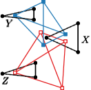
Let $P=\{p_{1},\dots,p_{n}\}$ be a set of $n$ points in the plane and let $C=\{C_{1},\ldots,C_{k}\}$ be a partition of $P$ into $k$ sets of points, called color classes, such that every point belongs to exactly one color class. We study the partition spanning forest problem which is defined as follows: Is there a crossing-free straight-line drawing of a spanning forest $F$ that consists of $k$ trees $T_{1},\ldots,T_{k}$ such that each tree $T_{i}$, $1\leq i\leq k$, contains exactly the points of the color class $C_{i}$? Figure 1 shows an example with three color classes.

For $k=1$, the problem is equivalent to finding a geometric spanning tree of $P$ which trivially always exists. Hence, several optimization versions of this problem have been studied in the past; see Eppstein [4] for a survey. Bereg et al. [3] showed how to solve the problem in $O(n\log n)$ time in the case of $k=2$. Hiu and Schaefer [5] proved that it is $\NP$-complete to decide for two color classes $A=\{a_{1},\ldots,a_{n}\}$ and $B=\{b_{1},\ldots,b_{n}\}$ whether there exists an ordering $\pi$ such that the geometric paths $a_{\pi_{1}},\ldots,a_{\pi_{n}}$ and $b_{\pi_{1}},\ldots,b_{\pi_{n}}$ are crossing-free. Bereg et al. [2] asked for not necessarily straight-line Steiner trees for each color class of minimum total length and gave a PTAS for $k=2$, a $(5/3+\varepsilon)$-approximation for $k=3$, and a $(k+\varepsilon)$-approximation for $k>2$.

In this paper, we analyze the complexity of the partition spanning forest problem for color classes of bounded size. We give an $O(n^{2})$-time algorithm when each color class contains at most three points (Sec. 2) and show that the problem is $\NP$-complete for up to five points per color class (Sec. 3); the complexity for four points remains open. In Section 4, we show that the partition spanning linear forest problem, where each tree is required to be a path, is $\NP$-complete, even if every color class contains at most four points. The complexity of the non-linear version remains open if every color class contains at most four points.

Figure 1: A solution to a problem instance with three color classes.

2 Color classes with at most three points

In the case where each color class of the input instance contains of at most three points, the partition spanning forest problem can be solved in polynomial time. In fact, with this restriction the problem can be formulated as a 2-SAT problem.

Assume that our point set $P=\{p_{1},\dots,p_{n}\}$ consists of $n$ points. In the following we will understand the color classes as subsets $I\subseteq[n]:=\{1,\dots,n\}$ of indices. For a point $p_{i}$ we denote its color class by $I(p_{i})$. We refer to the edges $(p_{i},p_{j})$ where $p_{i}$ and $p_{j}$ are in the same color class as the potential edges of the instance. Observe that an arbitrary choice of the potential edges forms a solution to the problem (with at most three points per color class) if and only if it satisfies the following conditions: (i) For each point $p_{i}$, if $|I(p_{i})|>1$, then at least one potential edge incident to $p_{i}$ must be chosen. (ii) For any pair of potential edges $p_{i}p_{j}$ and $p_{k}p_{l}$ that intersect in the interior, at most one of them is chosen. (iii) For any color class $I$ with $|I|=3$ one of the potential edges of that color is not chosen.

Observe that condition (iii) can be skipped, as any choice of potential edges satisfying conditions (i) and (ii) can be extended to also satisfy (iii).

We model the possible choices of potential edges that satisfy conditions (i) and (ii) by a 2-SAT formula as follows. For each potential edge $(p_{i},p_{j})$ there is a variable $x_{ij}$ with the interpretation that if $x_{ij}$ is true, then the edge connecting $p_{i}$ to $p_{j}$ is not chosen as part of the solution, and otherwise it is.

Conditions (i) and (ii) can be expressed as 2-SAT formulas using the variables $x_{ij}$ as follows. For condition (i), we create for each point $p_{i}$ the (sub)formula $\bigvee_{j\in I(p_{i})\setminus\{i\}}\lnot x_{ij}$. Note that this is a 2-SAT formula since $|I(p_{i})\setminus\{i\}|\leq 2$ by the assumption that each color class has size at most three. For any two potential edges $(p_{i},p_{j})$ and $(p_{k},p_{l})$ that cross, we add the clause $x_{ij}\vee x_{kl}$, thus enforcing condition (ii). It follows that the resulting 2-SAT formula $\varphi$ is satisfiable if and only if the original instance of the partition spanning forest problem admits a solution.

If a color class contains only one point, then we can always draw it as a singleton point since we assumed general position for our input points. Thus, we are left with sets of either two or three points. In the case of two points, there is a unique spanning tree. However, for sets with three points we have three choices. For each of those spanning trees, we introduce a boolean variable. In particular, if the color class is $\{p_{i},p_{j},p_{k}\}$, then we denote the boolean variable for the spanning tree formed by the edges $(p_{i},p_{j})$ and $(p_{j},p_{k})$ by $x_{ik}$, using its endpoints as the indices. The interpretation of the variable assignment will be the following: if $x_{ik}$ is true, then the corresponding spanning tree is selected as the spanning tree for its color class; if $x_{ik}$ is false, then any of the three possible spanning trees of its color class can be chosen. To make this work, we have to guarantee that at most one of $x_{ij},x_{jk}$, and $x_{ik}$ is true. This can be enforced by the 2-SAT (sub)formula

$$(\lnot x_{ij}\lor\lnot x_{ik})\land(\lnot x_{jk}\lor\lnot x_{ik})\land(\lnot x_{ij}\lor\lnot x_{jk}).$$

We add this formula for every color class with three elements.

In the next step, we process each pair of color classes. While processing, we will observe one of the following: (i) the local configuration already forbids the existence of a partition drawing, (ii) the two sets impose a constraint on the available spanning trees, or (iii) the two sets do not interfere with each other. In case of (i) we can stop the algorithm, in case of (ii) we (iteratively) build a 2-SAT formula to model these constraints.

Let now $A$ and $B$ be a pair of color classes. If $|A|=|B|=2$, then their convex hull is either intersecting or not. In the former case, there exists no partition drawing; in the latter, these two sets impose no constraints.

If one of the color classes contains three points (say $A$) and the other contains two points, then we are left with one of the following situations. The convex hulls of both sets could be disjoint, which yields no constraints. If two edges of the convex hull of $A$ are intersected by the convex hull of $B$, then there cannot be a spanning tree of $A$ avoiding the edge spanned by $B$. Thus, in this case we cannot have a partition drawing. Finally, if the segment spanned by $B$ intersects a single edge of the convex hull of $A$, then only one of the three possible spanning tress of $A$ can be part of a partition drawing. In this case, we add an appropriate clause to the 2-SAT formula that enforces the corresponding spanning tree.

We are left with the case that $|A|=|B|=3$. Clearly, if the convex hulls of these sets are disjoint, then this pair imposes no constraints. If their convex hulls intersect in four or even six points, it is an easy exercise to see that in this case a partition drawing is not possible. If there are two intersection points, we have to consider two cases. If both intersections lie on the same edge, say $(p_{i},p_{j})$ spanned by points from $A$, then only one spanning tree in $A$ can be chosen (see Figure 2(a)). In this case, we enforce $x_{ij}$ to be true by adding the clause $x_{ij}$ to the formula. In the remaining case, let $A=\{p_{i},p_{j},p_{k}\}$ and $B=\{p_{a},p_{b},p_{c}\}$. We assume that $(p_{i},p_{j})$ intersects $(p_{a},p_{b})$ and that $(p_{j},p_{k})$ intersects $(p_{b},p_{c})$. Now, we have two pairs of possible spanning trees (see Figure 2(b–c)). To model this, we add the clauses

$$(\lnot x_{ij}\lor\lnot x_{ab})\land(\lnot x_{jk}\lor\lnot x_{bc})$$

to our 2-SAT formula.

(a)

(b)

(c)

Figure 2: Local constraints for spanning trees. (a) A situation where one color class is restricted to one spanning tree. (b–c) Another situation where two depended spanning trees for each color class are possible.

By the above strategy, we have constructed a 2-SAT formula that is satisfiable if and only if the input instance has a partition drawing.

The formula has length at most $O(n^{2})$ and can be constructed in $O(n^{2})$ time as well. By using an efficient algorithm for 2-SAT [1], we get the desired algorithm. We summarize our construction in the following theorem.

Theorem 1.

The partition spanning forest problem for $n$ points can be solved in $O(n^{2})$ time if every color class contains at most three points.

3 Color classes with at most five points

In this section we prove the following theorem:

Theorem 2.

The partition spanning forest problem is $\NP$-complete, even if every color class contains at most five points.

The problem is obviously contained in $\NP$. In order to show the $\NP$-hardness, we perform a polynomial-time reduction from Planar 3-Satisfiability. In this $\NP$-hard [8] special case of 3SAT the input is a 3SAT formula $\varphi$ whose variable–clause graph is planar. We can assume that such a formula is given together with a contact representation $\mathcal{R}$ of $\varphi$ [7]. Thus, all variables are represented as horizontal line segments arranged on one line. Each clause $c$ is represented as an E-shape turned by $90^{\circ}$ such that the three vertical legs of the E-shape touch precisely the variables contained in $c$. For our reduction, we construct a set of colored points that admits a partition drawing if and only if $\varphi$ is satisfiable.

Overview.

We introduce five types of gadgets. For each variable $u$ we create a variable gadget which admits exactly two distinct partition drawings. These drawings correspond to the two truth states of $u$. Wire gadgets are used to propagate these states to the clause gadgets, one of which is created for every clause $c$. The clause gadget of $c$ ensures that gadget configurations of the variables contained in $c$ correspond to a truth assignment in which at least one of the literals of $c$ is satisfied. In order to connect our gadgets appropriately we also require a splitting gadget, which splits one wire into two wires, and we require a gadget that flips the state transported along a wire. We proceed by describing our gadgets in detail. Note that different gadgets always use different color classes, even if we might give them the same name in the construction (so there are many red color classes in an instance).

The wire gadget.

The wire gadget consists of four color classes; see Figure 3. The points of the red color class $R=\{r_{1},r_{2},r_{3}\}$ and the blue color class $B=\{b_{1},b_{2},b_{3}\}$ are arranged such that the convex hulls of $R$ and $B$ intersect in the two points $b_{1}b_{2}\cap r_{1}r_{2}$ and $b_{1}b_{3}\cap r_{1}r_{3}$. As a consequence, there are exactly two possible configurations for the red and blue spannings trees which can be used in a partition drawing, see Figure 3(a) and Figure 3(b). Either choice uniquely determines the spanning tree of both the green color class $G=(g_{1},\dots,g_{5})$ and the orange color class $O=(o_{1},\dots,o_{5})$, as the edges of the red and blue spanning trees obstruct all other possible green and orange edges. Thus, there are exactly two possible partition drawings of the wire gadget. In particular, these two drawings satisfy the following.

Observation 1.

Any partition drawing of the wire gadget either contains (i) the edges $g_{1}g_{2}$ and $o_{1}o_{2}$, but not the edges $g_{1}g_{3}$ and $o_{1}o_{3}$, see Figure 3(a); or (ii) the edges $g_{1}g_{3}$ and $o_{1}o_{3}$, but not the edges $g_{1}g_{2}$ and $o_{1}o_{2}$, see Figure 3(b).

(a) State (i)

(b) State (ii)

(c) A chain

Figure 3: The configurations of the wire gadget

These two states (i) and (ii) may be propagated by creating chains of wire gadgets in which the convex hulls of consecutive gadgets intersect in two points as illustrated in Figure 3(c). Consider two consecutive wire gadgets in a chain. By Observation 1, either both gadgets are in state (i) or both gadgets are in state (ii) due to the way their convex hulls intersect. As a consequence, the first gadget of the chain is in state (i) if and only if the last one is in state (i) as well. Chains are flexible structures and turns can easily be implemented by curving a chain. Further, the length of a chain may be adjusted by increasing or decreasing the distance between consecutive wire gadgets.

Splitting and inverting.

The splitting gadget consists of two color classes $V=\{v_{1},\dots,v_{5}\}$ (violet) and $P=\{p_{1},\dots,p_{5}\}$ (purple) whose points are placed between two consecutive wires $W_{1},W_{2}$ in a chain, see Figure 4. The functionality of these two color classes is similar to the one of the color classes green and orange in the wire gadget: the state of $W_{1}$ and $W_{2}$ uniquely determines the spanning tree of both the violet and the purple color class. In particular, the purple tree contains either $p_{1}p_{3}$ or $p_{1}p_{5}$ and the violet tree contains either $v_{1}v_{2}$ or $v_{1}v_{3}$. We may now attach one or two additional wires perpendicular to the chain such that their convex hulls intersect the convex hull of the splitting gadget, see $W_{3}$ and $W_{4}$ in Figure 4. The edges incident to $p_{1}$ and $v_{1}$ in the purple and violet spanning trees allow precisely one state for both $W_{3}$ and $W_{4}$.

Observation 2.

In any drawing of the splitting gadget, the state of the wires $W_{3}$ and $W_{4}$ differs from the state of $W_{1}$ and $W_{2}$.

Figure 4: Splitting gadget

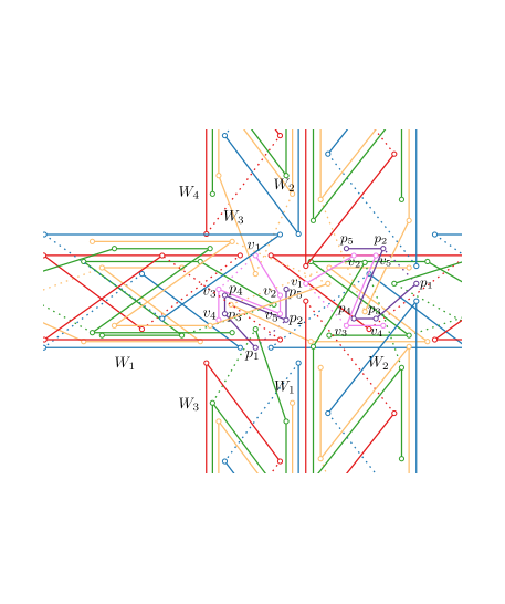
In this sense, the splitting gadget does not only split a wire into two wires, it can also be used to flip the state propagated along a chain.

The variable gadget.

The variable gadget is a horizontal chain to which we attach multiple wires using splitters. The number of wires attached from the top (bottom) matches the number of E-shape legs touching the variable from the top (bottom) in the contact representation $\mathcal{R}$ of $\varphi$.

The clause gadget.

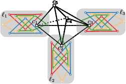
The clause gadget for a clause of three literals $\ell_{1},\ell_{2},\ell_{3}$ consists of one color class with exactly five vertices $c_{1},\ldots,c_{5}$. We place $c_{1},c_{2}$, and $c_{3}$ inside a wire gadget representing $\ell_{1},\ell_{2}$, and $\ell_{3}$, respectively, and we place $c_{4}$ and $c_{5}$ between those as depicted in Figure 5. We will now show that the gadget is drawable if and only if at least one of $\ell_{1},\ell_{2},\ell_{3}$ is true. In particular, we can always use an edge to connect $c_{4}$ and $c_{5}$. We can connect $c_{3}$ to $c_{4}$ if $\ell_{3}$ is true and we can connect $c_{3}$ to $c_{5}$ otherwise; similarly, we can connect $c_{2}$ to $c_{5}$ if $\ell_{2}=\textsc{true}$ and we can connect $c_{2}$ to $c_{4}$ otherwise. If $\ell_{1}=\textsc{true}$, then we can always connect $c_{1}$ to $c_{5}$. However, if $\ell_{1}=\textsc{false}$, then we cannot connect $c_{1}$ to $c_{4}$ or $c_{5}$, and we can connect it to $c_{2}$ or $c_{3}$ only if $\ell_{2}$ or $\ell_{3}$ is true, respectively. Hence, the gadget is not drawable if $\ell_{1}=\ell_{2}=\ell_{3}=$false. Note that the connection from $c_{1}$ to $c_{3}$ might intersect the connection from $c_{2}$ to $c_{4}$. However, we only have to use it if $\ell_{1}=\ell_{2}=\textsc{false}$ and $\ell_{3}=\textsc{true}$; in this case, we can connect $c_{2}$ to $c_{3}$ instead of $c_{4}$. Thus, the gadget is drawable if and only if at least one of $\ell_{1}$, $\ell_{2}$, and $\ell_{3}$ is true.

(a) $\ell_{1}=\ell_{2}=\ell_{3}=\textsc{true}$

(b) $\ell_{1}=\ell_{2}=\ell_{3}=\textsc{false}$

Figure 5: The clause gadget between literals $\ell_{1},\ell_{2},\ell_{3}$.

Layout and correctness.

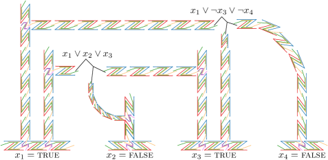
The wires that are attached to the variable gadgets are vertical and, by Observation 2, their state is inverted, so they propagate the negated variable. Hence, if a literal is positive, we have to invert the state of the wire again. Two of the wires are supposed to enter the clause horizontally; for these two, if they correspond to a positive literal, we simply use another splitting gadget to make the wire horizontal. Otherwise, the wire makes a $90^{\circ}$ degree turn to become horizontal and to propagate the negated variable. The third wire is supposed to enter the clause gadget vertically, so if its literal is negative, the vertical wire can directly connect to the clause. Otherwise, we use another splitting gadget followed by a $90^{\circ}$ degree turn. See Figure 6 for an example of that shows all cases. Since the clause gadgets are drawable if and only if one of their literals is true and since the wires propagate the states of the variable gadgets, the resulting instance is drawable if and only if the planar 3SAT formula $\varphi$ is satisfiable, which proves the correctness of Theorem 2.

Figure 6: A full example.

4 Linear forests for color classes with at most four points

In this section we consider the additional restriction that the spanning forest is a linear forest, that is, each connected component is a path. Note that, if every color class contains at most three points, then every spanning forest is linear, so in this case we can solve the problem in polynomial time. On the other hand, we show that under this additional restriction, the problem is $\NP$-complete already if every color class contains at most four points.

Theorem 3.

The partition spanning linear forest problem is $\NP$-complete, even if every color class contains at most four points.

Again, the problem is clearly contained in $\NP$. In order to show the $\NP$-hardness, we again perform a polynomial-time reduction from Planar 3-Satisfiability, but using different gadgets. As before, we construct a variable gadget, a splitting gadget, a wire gadget, and an inverter gadget. Instead of directly constructing a clause gadget, we will however construct an OR-gadget. The clause gadget can then be built by concatenating two OR-gadgets and enforcing the resulting variable gadget to be set to true by crossing the appropriate edge with a new color class consisting of two points.

The variable, wire, and inverter gadgets.

The variable gadget consists of one color class, the black color class $X=\{x_{1},x_{2},x_{3}\}$. Using a second color class, the blue color class $B=\{b_{1},b_{2},b_{3}\}$, we can enforce that the edge $x_{1}x_{2}$ must be drawn in any partition drawing. The classes $B$ and $X$ are placed in such a way that their convex hulls intersect in two points. In particular, there are two distinct partition drawings for $B$ and $X$, corresponding to two truth states and $x_{1}x_{2}$ is present in both of them.

Figure 7: The wire gadget.

(a)

(b)

(c)

Figure 8: The splitting gadget and its assignments.

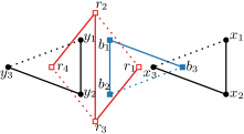
The wire gadget consists of four color classes, the red color class $R=\{r_{1},r_{2},r_{3},r_{4}\}$ and the blue color class $B=\{b_{1},b_{2},b_{3}\}$, and two black color classes $X=\{x_{1},x_{2},x_{3}\}$ and $Y=\{y_{1},y_{2},y_{3}\}$, see Figure 7. Classes $B$ and $X$ are placed as in the variable gadget. Class $Y$ is a copy of $X$, placed outside the convex hull of $X$ and $B$. The point $r_{1}$ is placed inside the convex hull of $B$ but outside the convex hull of $X$. The point $r_{4}$ is placed inside the convex hull of $Y$ and $r_{2}$ and $r_{3}$ are placed such that the line through them separates the convex hulls of $B$ and $Y$. Then, either partition drawing on $X$ and $B$ induces a unique partition drawing of $R$ and $Y$, where the drawing on $Y$ is the same as the drawing on $X$.

Placing $Y$ as a copy of $B$ instead of $X$, i.e., with only one point in the convex hull of $R$, we can also turn this gadget into an inverter gadget.

The splitting gadget.

The splitting gadget consists of three variable gadgets $X$, $Y$, and $Z$, and two additional color classes, the red color class $R$ and the blue color class $B$, see Figure 8. The truth assignment on $X$ enforces some edges in $R$ and $B$ to be present, which then uniquely determines the partition drawing on the whole gadget. Note that the truth assignments on $Y$ and $Z$ are enforced as the negated truth assignment on $X$, so an additional inverter gadget might be needed depending on the required literal.

The OR-gadget.

The OR-gadget consists of three variable gadgets $X$, $Y$, and $Z$, and two additional color classes, the red color class $R$ and the blue color class $B$, see Figure 9. The truth assignments on $X$ and $Y$ enforce some edges in $R$ and $B$ to be present. It can be seen that the drawing of $Z$ corresponding to the value true can only be drawn if $X$ or $Y$ are also drawn corresponding to the value true. In some of these cases, $Z$ could also be drawn according to the value false, but this does not affect the proof as it is still true that the constructed point set admits a partition drawing if and only if the planar 3SAT formula $\varphi$ is satisfiable.

Figure 9: Assignments of the OR-gadget.

References

- [1] Bengt Aspvall, Michael F. Plass, and Robert E. Tarjan. A linear-time algorithm for testing the truth of certain quantified boolean formulas. Inform. Process. Lett., 8(3):121–123, 1979. doi:10.1016/0020-0190(79)90002-4.
- [2] Sergey Bereg, Krzysztof Fleszar, Philipp Kindermann, Sergey Pupyrev, Joachim Spoerhase, and Alexander Wolff. Colored non-crossing euclidean steiner forest. In Khaled M. Elbassioni and Kazuhisa Makino, editors, Proc. 26th Int. Symp. Alg. Comput. (ISAAC’15), volume 9472 of Lecture Notes Comput. Sci., pages 429–441. Springer, 2015. doi:10.1007/978-3-662-48971-0_37.
- [3] Sergey Bereg, Minghui Jiang, Boting Yang, and Binhai Zhu. On the red/blue spanning tree problem. Theor. Comput. Sci., 412(23):2459–2467, 2011. doi:10.1016/j.tcs.2010.10.038.
- [4] David Eppstein. Spanning trees and spanners. In Jörg-Rudiger Sack and Jorge Urrutia, editors, Handbook Comput. Geom., chapter 9, pages 425–461. Elsevier, 2000. URL: http://www.ics.uci.edu/~eppstein/pubs/Epp-TR-96-16.pdf.
- [5] Peter Hui and Marcus Schaefer. Paired pointset traversal. In Rudolf Fleischer and Gerhard Trippen, editors, Proc. 15th Int. Symp. Alg. Comput. (ISAAC’04), volume 3341 of Lecture Notes Comput. Sci., pages 534–544. Springer, 2004. doi:10.1007/978-3-540-30551-4_47.
- [6] Philipp Kindermann, Boris Klemz, Ignaz Rutter, Patrick Schnider, and André Schulz. The partition spanning forest problem. In Matias Korman and Wolfgang Mulzer, editors, Proc. 34th Europ. Workshop Comput. Geom. (EuroCG’18), pages 53:1–53:6. FU Berlin, 2018. Extended Abstract. URL: https://conference.imp.fu-berlin.de/eurocg18/download/eurocg_proc.pdf.
- [7] Donald E. Knuth and Arvind Raghunathan. The problem of compatible representatives. SIAM J. Discrete Math., 5(3):422–427, 1992. doi:10.1137/0405033.
- [8] David Lichtenstein. Planar formulae and their uses. SIAM J. Comput., 11(2):329–343, 1982. doi:10.1137/0211025.