Geometric goodness of fit measure to detect patterns in data point clouds

Abstract

We derived a geometric goodness-of-fit index, similar to $R^{2}$   using topological data analysis techniques. We build the Vietoris-Rips complex from the  data-cloud projected onto each variable. Estimating the area of the complex and their domain,    we create an index that measures the emptiness of the space with respect to the data. We made the analysis with an own package    called TopSA (Topological Sensitivy Analysis).

Introduction

Data point cloud recognition is an essential task in any statistical procedure. Finding a pattern into the data expose the inherent characteristics of the phenomena we want to model. There are tools described in the literature  like linear regression or clustering  used to achieve this Hastie2009 ; Hand2005 . Other research branches use data visualization techniques to highlight features hidden in the data Tufte2001 ; Myatt2009 ; Buja2005 .

Professionals in computational modeling aim to reduce their models by choosing their problems’ most relevant factors. One way to achieve this is through goodness-of-fit measures, used to find the relevance of certain chosen models to explain a variable.  One classic way to determine if  some variables fit inside a model is using the determination coefficient $R^{2}$. This quantity measures the amount of variance explained by some model against the variance explained by the model formed only by a constant.  It measures how preferable it would be to fit a model against just fitting  a  constant.  If $R^{2}$ is near  one, then the model fits well into the data. Otherwise it is better to adjust to a constant.

The $R^{2}$ method  has been controversial since its origins Barrett1974 . For example, we can increase the $R^{2}$ score by adding new variables to the model. Even if they are unnecessary to the problem the $R^{2}$ will increase. As a general rule, high $R^{2}$ does not imply causation between covariance and outcome.

Some authors have proposed some extensions and properties of this score throughout the years. The work of Barten1962 presents a bias-reduced $R^{2}$. In Press1978 the authors conducted a Bayesian analysis. In  Cramer1987 the authors showed that in small samples, the $R^{2}$ score is higher. Even with those constraints, Barrett1974 concludes how useful are these measures in applied research.

This goodness-of-fit measures overlook the geometric arrangement of the data. They build the statistical relation between $X$ and $Y$ and then present it in the form of an indicator. Depending on this simplification, they do not consider the geometric properties of the data. For example, most indices will cannot recognize geometric structure when the input variable is zero-sum, treating it as random noise.

The study of topological data is a recent field of research that aims to overcome these shortcomings. Given a set of points generated in space, it tries to reconstruct the model through an embedded manifold that covers the data set. With this manifold, we can study the characteristics of the model using topological and geometrical tools instead of using classic statistical tools.

Two classical methods used to describe the intrinsic geometry of the data are Principal Components Analysis (PCA) and Multidimensional Scaling (MDS). PCA transforms the data into a smaller linear space, preserving the statistical variance. MDS performs the same task but preserves the distances between points. Methods like the isomap algorithm developed in Tenenbaum2000 and expanded in Bernstein2000 and Balasubramanian2002 unify these two concepts to allow the reconstruction of a low-dimensional variety for non-linear functions. Using geodesic distance, isomap identifies the corresponding manifold and searches lower dimensional spaces.

In recent years new theoretical developments have used theorical ideas in topology for the data analysis. Such  ideas include persistent homology, simplicial complexes, and Betti numbers. Reconstructing manifolds work for clouds of random data and functional data. The following works present some examples: Ghrist2008 , Carlsson2009 and Carlsson2014 . In Gallon2013 and in Dimeglio2014 . Also, this approach compacts “Big Data” problems efficiently  (see  Snasel2017 ).

In this work we aim to connect the concept of goodness of fit with the analysis of topological data  through a geometrical $R^{2}$ index. By doing this it will be possible to determine what variables have structured patterns using the geometrical information extracted from the data.

The outline of this study is: Section 1 deals with key notions, both in sensitivity analysis and in topology. In Subsection 1.1 wer review and comment classic methods to determine the $R^{2}$. We finish this subsection with an example which motivated the work in this paper. Subsection 1.2 deals with preliminaries in homology and describes the Vietoris-Rips Complex. Section 2 explains the method used to create our sensitivity index; Subsection 2.1 constructs the neighborhood graph, and deals with different topics such as the importance of scale, the Ishigami Model and presents programming code to determine the radius of proximity. Subsection 2.2 describes the algorithm used to construct the homology complex through the Vietoris-Rips  complex and Subsection 2.3 explains our proposed sensitivity index. Section 3 describes our results, it describes the software and packages used to run our theoretical examples. Subsection 3.1 is a full description of each theoretical example together with visual aids, such as graphics and tables describing the results. Section 4 contains our conclusions and explores scenarios for future research.

1 Preliminary Aspects

In this section we will discuss the context and tools needed to implement our geometric goodness-of-fit.

1.1 Measuring goodness-of-fit

Let $(X_{1},X_{2},\ldots X_{p})\in\mathbb{R}^{p}$ for $p\geq 1$ and $Y\in\mathbb{R}$ two random variables. Define the non-linear regression model as

$$Y=\varphi(X_{1},X_{2},\ldots X_{p})+\varepsilon,$$ (1)

where $\varepsilon$ is random noise independent of $(X_{1},X_{2},\ldots X_{p})$. The unknown function $\varphi:\mathbb{R}^{p}\mapsto\mathbb{R}$ describes the conditional expectation of $Y$ given $(X_{1},X_{2},\ldots X_{p})$. Suppose as well that $(X_{i1},X_{i2}\ldots X_{ip},Y_{i})$, for $i=1,\ldots,n$, is a size $n$ sample for the random vector$(X_{1},X_{2}\ldots X_{p},Y)$.

If $p\gg n$ the model (1) suffers from the “curse of dimensionality”, term introduced in Bellman1957 and  Bellman1961 , where is shown that the sample size $n$, required to fit a model increases with the number of variables $p$. Model selection techniques solve this problem using indicators as the AIC or BIC, or more advanced techniques such as Ridge or Lasso regression. For the interested reader there is a comprehensive survey in Hastie2009 .

Suppose in the context of the linear regression we have the model

$$\mathbf{Y}=\mathbf{X}\mathbf{b}+\boldsymbol{\varepsilon}$$

where

$$\mathbf{Y}=\begin{pmatrix}Y_{1}\\ \vdots\\ Y_{n}\end{pmatrix},\ \mathbf{X}=\begin{pmatrix}1&X_{11}&X_{12}&\cdots&X_{1p}\\ \vdots&&\vdots&&\vdots\\ 1&X_{n1}&X_{n2}&\cdots&X_{np}\\ \end{pmatrix},\ \mathbf{b}=\begin{pmatrix}b_{0}\\ \vdots\\ b_{p}\end{pmatrix},\ \boldsymbol{\varepsilon}=\begin{pmatrix}\varepsilon_{1}\\ \vdots\\ \varepsilon_{n}\end{pmatrix}$$

and $\boldsymbol{\varepsilon}$ is a noisy vector with mean $(0,\ldots,0)^{\top}$ and identity covariance.

The least-square solutions to find the best coefficients is

$$\mathbf{\hat{b}}=\left(\mathbf{X}^{\top}\mathbf{X}\right)^{-1}\mathbf{X}^{\top}\mathbf{Y}.$$

If $p=1$ the problem reduces to the equations,

$$\hat{b}_{i1} =\frac{\sum_{j=1}^{n}\left(X_{ij}-\bar{X}_{i}\right)\left(Y_{j}-\bar{Y}\right)}{\sum_{j=1}^{n}\left(X_{ij}-X_{i}\right)^{2}}$$

$$\hat{b}_{i0} =\bar{Y}-\hat{b}_{1}\bar{X}_{i}$$

Notices that in the particular case $p=0$ (the null model) then the estimated parameter simplifies into $\hat{b}_{0i}=\bar{Y}$.

The following identity holds in our context,

$$\sum_{j=1}^{n}\left(Y_{j}-\bar{Y}\right)^{2} =\sum_{j=1}^{n}\left(\hat{Y}_{j}-\bar{Y}\right)^{2}+\sum_{j=1}^{n}\left(\hat{Y}_{j}-Y_{j}\right)^{2}$$

One of the most used quantities to quantify if one covariate (or a set of them) are useful to explain an output variable is the statistic $R^{2}\in[0,1]$. We estimate it as

$$R^{2}=1-\frac{\sum_{j=1}^{n}\left(\hat{Y}_{j}-Y_{j}\right)^{2}}{\sum_{j=1}^{n}\left(Y_{j}-\bar{Y}\right)^{2}}$$

This value indicates how much the variability of the regression model explains the variability of $Y$. If $R^{2}$ is close to zero, the squared residuals of the fitted variables are similar to the residuals of a null model formed only by a constant. Otherwise, the residuals of the null model are greater than the residuals of the fitted values, meaning that the selected model could approximate better the observed values of the sample.

The $R^{2}$ has the deficiency that it increases if we add new variables to the model. A better statistic to measure the goodness of fit but penalizing the inclusion of nuisance variable is the Adjusted $R^{2}$,

$$R^{2}_{Adj}=1-(1-R^{2})\frac{n-1}{n-p-1}$$

These measures could detect if a data point cloud could be fitted through some function. However, if the structure of the data has anomalous patterns $R^{2}$ could be insufficient.

For example Figure 1 presents this phenomena for two data sets. We adjusted a polynomial of degree 8 to each set using least-square regression; the “Ishigami” and “Circle with one hole” models are presented in Section 3.

The Ishigami model presents strong non-linearity in its second variable. The model could capture the relevant pattern of the data and we got a $R^{2}=0.448$ and $R^{2}_{Adj}=0.4435$ (panel (c)). This tells us that we could capture around the 44% of the total variability of the data. We point out that classic regression failed to capture any of geometric features. In particular the $R^{2}$ and $R^{2}_{Adj}$ are near to zero.

Figure 1: Linear regression $Y=a_{0}+a_{1}X$ with (a) Ishigami model, and (b) Circle with hole model. Polynomial regression $Y=a_{0}+\sum_{k=1}^{8}a_{k}X_{1}^{k}$ with (c): Ishigami model (d): Circle with one hole model.

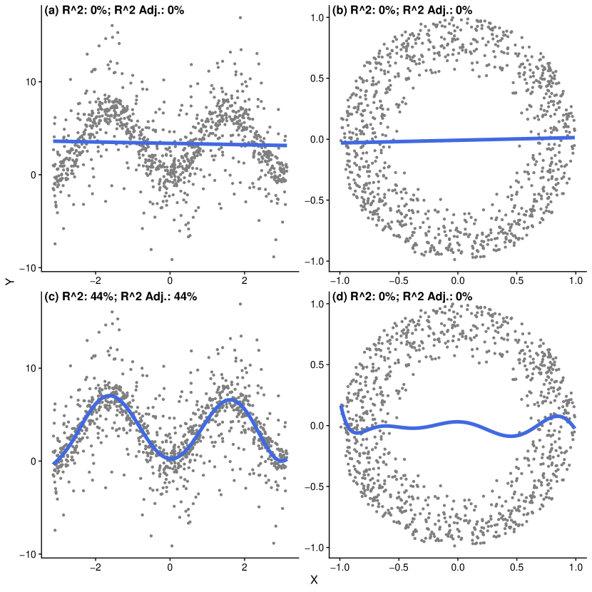
The issue with panels (a), (b) and (d) in Figure 1 is that the fitted models are inflexible with respect to the data that we used. In particular, the “Circle with one hole” model requires a better understanding about the anomalous geometry of the data cloud. The next Section explores how to better determine the geometric structure of the data to overcome this shortcomings.

1.2 Homology and Vietoris-Rips Complex

The seminal work of Carlsson2014 presents the ground basic definitions to define a homological structure for a data cloud of points. In particular, we are interested in the reconstruction of the embedding manifold of the cloud of points using only the distance between each pair of points.

For the purpose of this paper a geometric object is either a connected surface or connected directed graph. Given a geometric object define a $0$-simplex as a point, frequently called a vertex. Since we deal with finite sets of data, taking coordinates on the Euclidean Plane $\mathcal{E}=\mathbb{R}^{2}$, we denote a $0$-simplex as a point $p_{j}=(x_{j},y_{j})$ for $j=1,\ \dots,\ n$.

If we join two distinct $0$-simplices, $p_{0},p_{1}$, by an oriented line segment, we get a $1$-simplex called an edge: $\overline{p_{0}p_{1}}=(p_{1}-p_{0})$.

Consider now three non-colinear points $p_{0},\ p_{1},\ p_{2}$ as $0$-simplices, together they form three $1$-simplices: $\overline{p_{0}p_{1}}$, $\overline{p_{0}p_{2}}$ and $\overline{p_{1}p_{2}}=\overline{p_{0}p_{2}}-\overline{p_{0}p_{1}}$. This last equation shows that only two of them are linearly independent and span the other. The union of these three edges form a triangular shape, a $2$-simplex called a face, denoted as $\triangle(p_{0}p_{1}p_{2})$ that contains all the points enclosed between the edges:

$$\triangle(p_{0}p_{1}p_{2})=\Big{\{}p\in\mathbb{R}^{2}\colon p=\sum_{j=0}^{2}\lambda_{j}p_{j}\colon\sum_{j=0}^{2}\lambda_{j}=1,\lambda_{j}\geq 0\Big{\}}.$$

As well as $2$-simplices, if we consider four non-coplanar points on the Euclidean Space $\mathbb{R}^{3}$, we can construct a $3$-simplex called tetrahedron. A generalization of dimension $n$ will be a convex set in $\mathbb{R}^{n}$ containing $\left\{p_{0},p_{1},\dots,p_{n}\right\}$ a subset of $n+1$ distinct points that do not lie in the same hyperplane of dimension $n-1$ or, equivalently, that the vectors $\left\{\overline{p_{0}p_{j}}=p_{j}-p_{0}\right\},0<j\leq n$ are linearly independent. In such a case, we are denoting the points $\left\{p_{0},p_{1},\dots,p_{n}\right\}$ as vertices, and the usual notation would be $[p_{0},p_{j}]$ for edges, $[p_{0},p_{1},p_{2}]$ for faces, $[p_{0},\dots,p_{4}]$ for tetrahedra, and $[p_{0},\dots,p_{n}]$ for $n$-simplices. Nevertheles, for our purposes, it will be enough to consider just $0,\ 1$ and $2$-simplices, the latter constituting the building blocks of the Vietoris-Rips complex.

A $\bigtriangleup$-complex is the topological quotient space of a collection of disjoint simplices identifying some of their faces. This complex will be ordered in the sense that each vertex is in lexicographic order. In other words, there exists an injective mapping between $\left\{p_{0},\ldots,p_{n}\right\}$ and $\mathbb{N}$.

For any $n-$simplex $\sigma=[p_{0},\dots,p_{n}]$ the boundary of $\sigma$ is the the linear combination of $(n-1)$-simplices of the form

$$\partial_{n}\sigma=\sum_{j=0}^{n}(-1)^{j}[p_{0},\dots,\hat{p}_{j},\dots,p_{n}]$$ (2)

where

$$[p_{0},\dots,\hat{p}_{j},\dots,p_{n}]=[p_{0},\dots,p_{j-1},p_{j+1},\dots,p_{n}].$$

Hence, give our oriented simplicial complex, of dimension $n$, we can build a sequence of vector spaces and linear maps of the form,

$$\dots\to\bigtriangleup_{n}(X)\xrightarrow{\partial_{n}}\bigtriangleup_{n-1}(X)\xrightarrow{\partial_{n-1}}\bigtriangleup_{n-2}(X)\to\dots\to\bigtriangleup_{1}(X)\xrightarrow{\partial_{1}}\bigtriangleup_{0}(X)\xrightarrow{\partial_{0}}0$$

where $\partial\circ\partial=\partial_{n}\circ\partial_{n-1}=0$ for all $n$. This is usually known as a chain complex. Since $\partial_{n}\circ\partial_{n-1}=0$, the $\operatorname{Im}(\partial_{n})\subseteq\ker(\partial_{n-1})$, and so, we define the $n^{th}$ simplicial homology group of $X$ as the quotient

$$H_{n}^{\bigtriangleup}(X)=\frac{\ker(\partial_{n})}{\operatorname{Im}(\partial_{n+1})}.$$ (3)

The elements of the kernel are known as cycles and the elements of the image are known as boundaries.

The $n^{th}$-Betti number of $X$ is the rank of each space $H_{n}^{\bigtriangleup}(X)$. Roughly speaking, the $n$-th Betti number represents the number of $n$-dimensional holes on the topological surface. Formally, from the algebraic topology stand point of view, the first Betti numbers is $b_{0}$, that represents the number of connected components of the manifold; the second one is $b_{1}$, that represents the number of loops (circles) that span $H_{1}$ or informally, the number of circular holes ($1$-dimensional holes) on the manifold, and $b_{2}$ that represents the number of voids, $2$-dimensional holes. The reader may see Hatcher2000 or book:72583 for details.

Clarified those concepts, we can now define what is Vietoris-Rips complex.

Definition 1 (VR neigboorhood graph)

Given a sequence of vertices $\{p_{0},\ldots,p_{n}\}$ $\subseteq$ $\mathbb{R}^{n}$ and some positive value $\varepsilon\in\mathbb{R}$, the VR neighborhood graph is defined as $G_{\varepsilon}(V)=(V,E_{\varepsilon}(V))$ where

$$V =\{p_{0},\ldots,p_{n}\}$$

$$E_{\varepsilon}(V) =\{\{u,v\}\ \mid\ d(u,v)\leq\varepsilon,u\neq v\in V\},$$

represent the vertices and edges respectively.

Definition 2 (VR expansion)

Given a neighborhood graph $G_{\varepsilon}(V)$, their Vietoris-Rips complex $\mathcal{R}_{\varepsilon}$ is defined as all the edges of a simplex $\sigma$ that are in $G_{\varepsilon}(V)$. In this case $\sigma$ belongs to $\mathcal{R}_{\varepsilon}$. For $G_{\varepsilon}(V)=(V,E_{\varepsilon}(V))$, we have

$$\mathcal{R}_{\varepsilon}=V\cup E_{\varepsilon}(V)\cup\left\{\sigma\mid{\binom{\sigma}{2}}\subseteq E_{\varepsilon}(V)\right\}.$$

where $\sigma$ is a simplex of $G$.

1.3 Persistent Homology

There are two classical mistakes that can be made when start working with homological complexes. The first one, trying to find the optimal value for the radio $\varepsilon$, the homology of the complex associated to a point cloud data at a specific radio will be not enough. The second one, Betti numbers will be insufficient: we need a tool that tells us which holes we can keep and which holes we can ignore; classic homological constructions do not have that flexibility.

Persistence is a solution to this problem. The concept of persistence was introduced by Carlsson Carlsson2009 , Carlsson and Zomorodian Zomorodian2005 , and Zomorodian Zomorodian2010 , and also presented by Ghrist Ghrist2008 . Consider a parametrized family of spaces, for instance a sequence of Rips complexes $\{\mathcal{R}_{j}\}_{j=1}^{n}$ associated to a specific point cloud data for an incresaing sequence of radii $(\varepsilon_{j})_{j=1}^{n}$. Instead of considering the individual homology of the complex $\mathcal{R}_{j}$, consider the homology of the inclusion maps

$$\mathcal{R}_{1}\xrightarrow{i}\mathcal{R}_{2}\xrightarrow{i}\dots\mathcal{R}_{n-1}\xrightarrow{i}\mathcal{R}_{n}$$

i.e., consider he homology of the iterated induced inclusions

$$i_{*}\colon H_{*}(\mathcal{R}_{j})\to H_{*}(\mathcal{R}_{k})\quad\textmd{for}\quad j<k.$$

These induced homology maps will tell us which topological features persist. The persistence concept tell us how Rips complexes become a good approximation to C̆ech complexes (For full details see DeSilva2007 , Zomorodian2005 ).

Lemma 1 (Lemma 2.1.Ghrist2008 )

For any radio $\varepsilon>0$ there are inclusions

$$\mathcal{R}_{\varepsilon}\hookrightarrow\mathcal{C}_{\varepsilon\sqrt{2}}\hookrightarrow\mathcal{R}_{\varepsilon\sqrt{2}}.$$

To work with persistent homology in general, start considering a persistence complex $\{C_{*}^{i}\}_{i}$ which is a sequence of chain complexes joint with chain inclusion maps $f^{i}\colon C_{*}^{i}\to C_{*}^{i+1}$, according to the tools we are working with, we can take a sequence of Rips or C̆ech complexes of increasing radii $(\varepsilon_{j})_{j}$.

Definition 3

For $j<k$, we define the $(j,k)$-persistent homology of the persistent complex $C=\{C_{*}^{i}\}_{i}$ as the image of the induced homomorphism $f_{*}\colon H_{*}(C_{*}^{j})\to H_{*}(C_{*}^{k})$. We denote it by $H^{j\to k}_{*}(C)$.

A final ingredient will be needed. The barcodes are graphical representations of the persistent homology of a complex $H^{j\to k}_{*}(C)$ as horizontal lines in a $XY$-plane whose corresponds to the increasing radii $\{\varepsilon_{j}\}_{j}$, and whose vertical $Y$-axis corresponds to an ordering of homology generators. Roughly speaking, a barcode is the persistent topology analogue to a “Betti number”.

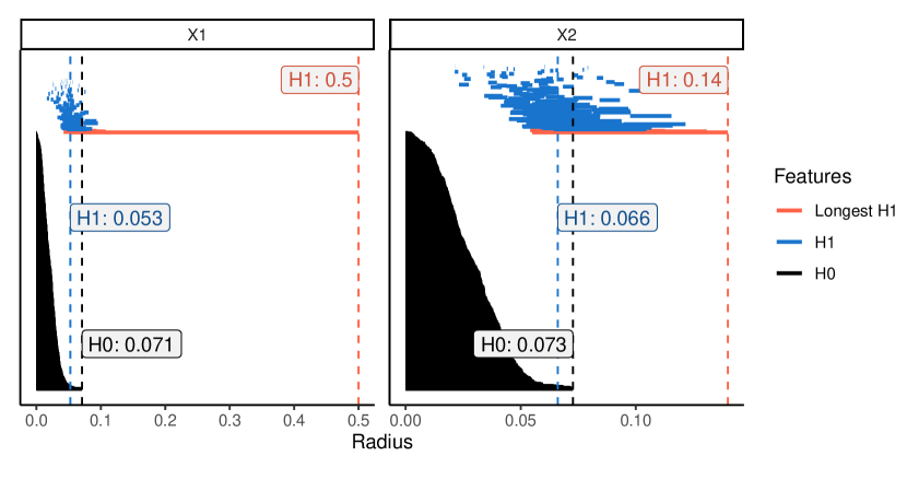
Figure 2 represent the barcodes for the example of a circle with a hole from Figure 1. Notices how the central hole persist on the left side plot (long $H_{1}$ red lines) while the noise it is  characterized by short lines in $H_{1}$.

Figure 2: Barcode representing the topological features of Figure r̃effig:fittedR2

2 Methodology

Recall the model (1). The random variables $(X_{1},\ldots,X_{p})$ are distorted by the function $m$ and its topology. Our aim is to measure how much each of the $X_{i}$ influence this distortion, i.e. we want to determine which variables influence the model the most.

In Section 1.1 we reviewed classical statistics methods to estimate the correspondence between random variables $X_{i}$, for $i=1,\ldots,p$, with respect to a model $Y$. In this paper we consider the geometry of the point-cloud, its enveloping manifold, and create an index that reveals information about the model.

The first step is to create a neighborhood graph for the point-cloud formed by $(X_{i},Y)$ where an edge is set if a pair of nodes are within $\varepsilon$ euclidean distance. In this way we connect only the nodes nearby within a fixed distance. With this neighborhood graph we construct the persistent homology using the method of Zomorodian2010 for the Vietoris-Rips (VR) complex.

The algorithm of Zomorodian2010 works in two-phases: First it creates a VR neighborhood graph (Definition 1) and then builds the VR complex step-by-step (Definition 2).

The definitions imply a two-phase procedure to construct the Vietoris-Rips complex with resolution $\varepsilon$:

1. Using Definition 1 compute the neighborhood graph $G_{\varepsilon}(V)$ with parameter $\varepsilon$.

2. Using Definition 2 compute $\mathcal{R}_{\varepsilon}$.

This procedure provides us with a geometrical skeleton for the data cloud points with resolution $\varepsilon$. In case the parameter $\varepsilon$ is large, there will be more edges connecting points. We could have a large interconnected graph with little information. Otherwise, if the parameter $\varepsilon$ is small, there may be fewer edges connecting the points, resulting in a sparse graph and missing relevant geometric features within the data cloud.

In the second step we unveil the topological structure of the neighborhood graph through the Vietoris-Rips complex. The expansion builds the cofaces related to our simplicial complex. In Section 2.2 we will further discuss the algorithm to achieve this.

2.1 Neighborhood graph

The neighborhood graph collects the vertices $V$ and for each vertex $v\in V$ it adds all the edges $[v,u]$ within the set $u\in V$, satisfying $d(v,u)\leq\varepsilon$. This brute-force operation works in $O(n^{2})$ time. We considered a variety of theoretical examples and it becomes clear that the scale factor in the data set is relevant. The scale in one variable may differ with the scale of the output by many orders of magnitude. Thus, proximity is relative to the scale of the axis on which the information is presented and the proximity neighborhood may be misjudged.

The Ishigami model presented in Figure 3 below shows how the proximity neighborhood becomes distorted when scale is taken into consideration.

Figure 3: The Second variable of the Ishigami model scaled to $[0,1]$ with a circle centered at $(0.5,0.5)$ and radius 1 (left). The same circle draw at the true scale of the data (right).

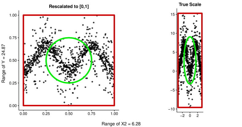
We conclude that the aspect ratio between both variables defines how the algorithm constructs the neighborhood graph. Therefore, to use circles to build the neighborhood graph we would need to set both variables to the same scale. Algorithm 1 constructs the VR-neighborhood graph for a cloud of points with arbitrary scales.

Data: A set of points $X=(X_{1},\ldots,X_{n})$ and $Y=(Y_{1},\ldots,Y_{n})$

A value $0<\alpha<1$.

Result: The Neighborhood Graph.

1

2 Function Create-VR-Neighborhood$((X,Y)$, $\alpha$):

3      $\displaystyle X_{r}\leftarrow\frac{X-\min{X}}{\max{X}-\min{X}}$

4       $\displaystyle Y_{r}\leftarrow\frac{Y-\min{Y}}{\max{Y}-\min{Y}}$

5       $n\leftarrow\mathrm{length}(Y)$

6       DistanceMatrix $\leftarrow$ Matrix$(n\times n)$

7      for i = 1:n do

8            for j = 1:n do

9                  DistanceMatrix[i,j] $\leftarrow$ $\sqrt{{(X_{r}\mathrm{[i]}-X_{r}\mathrm{[j]})}^{2}+{(Y_{r}\mathrm{[i]}-Y_{r}\mathrm{[j]})}^{2}}$

10             end for

11            

12       end for

13      $\varepsilon$ $\leftarrow$ Quantile (DistanceMatrix, $\alpha$)

14       AdjacencyMatrix $\leftarrow$ DistanceMatrix $\leq\varepsilon$

15      

16      NeighborhoodGraph $\leftarrow$ CreateGraph (AdjacencyMatrix, xCoordinates = $X$, y Coordinates = $Y$)

17      return (NeighborhoodGraph)

18 end

19

Algorithm 1 Procedure to estimate the neighborhood graph given a set of points in the plane.

1. Re-scale the points $(X_{i},Y)$, $i=1,\ldots,n$, onto the square $[0,1]\times[0,1]$.

2. Estimate the distance matrix between points.

3. With the distance chart estimate the $\alpha$ quantile of the distances. Declare the radius $\varepsilon_{i}$ as this quantile.

4. Using Definition 2 build the VR-neighborhood graph with $\varepsilon$ changed by $\varepsilon_{i}$ for each projection.

2.2 VR expansion

In Zomorodian2010 the author describes three methods to build the Vietoris-Rips complex. The first approach builds the complex by adding the vertices, the edges and then increasing the dimension to create triangles, tetrahedrons etc. The second method starts with an empty complex and adds all the simplices step-by-step stopping at the desired dimension. In the third method one takes advantage of the fact that the VR-complex is the combination of cliques in the graph of the desired dimension.

Due to its simplicity we adopt the third approach and detect the cliques in the graph. We use the algorithm in Eppstein2010 which is a variant of the classic algorithm from Bron1973 . This algorithm orders the graph $G$ and then computes the cliques using the Bron-Kerbosch method without pivoting. This procedure reduces the worst-case scenario from time $\mathcal{O}(3^{n/3})$ to time $\mathcal{O}(dn3^{d/3})$ where $n$ is the number of vertices and $d$ is the smallest value such that every nonempty sub-graph of $G$ contains a vertex of degree at most $d$.

Constructing a manifold via the VR-complex is not efficient in that the co-faces may overlap, increasing the computational time. One can overcome this by creating an ordered neighborhood graph.

2.3 Geometrical goodness-of-fit construction

The main use of the $R^{2}$ method is to gauge the variability explained by a chosen model against a null one. In our case, the null model is the box containing the Vietoris-Rips complex of our data. This is how we envelop the data in the most basic way possible. Our model will be the Vietoris-Rips complex itself, since it gives us a representation of our data through an identifiable structure.

The patterns in the data emerge through the empty spaces in the projection space generated by each individual variable. When the point-cloud fills the whole domain the unknown function $\varphi$ applied to $X_{i}$ produces erratic $Y$ values. Otherwise, the function yields a structural pattern which can be recognized geometrically.

The VR-complex $\mathcal{R}$ estimates the geometric structure of the data by filling the voids in-between close points. We may then estimate the area of the created object. This value will not yield too much information about the influence of the variable within the model. Therefore, we have to estimate the area of the minimum rectangle containing the entire object. If some input variable presents a weak correlation with the output variable, its behavior will be almost random with uniformly distributed points into the rectangular box. For the other cases, when there is some relevant correlation, it will create a pattern causing empty spaces to appear across the box.

To clarify the notation we will denote by $G_{\varepsilon,i}$ the neighborhood graph generated by the pair of variables $(X_{i},Y)$ and radius $\varepsilon$. Denote by $\mathcal{R}_{i}$ the VR-complex generated by $G_{\varepsilon,j}$. We also denote the geometrical area of the object formed by the VR-complex $\mathcal{R}_{i}$ by $\mathrm{Area}(\mathcal{R}_{i})$.

We define the rectangular box for the projection the data $(X_{i},Y)$ as

$$B_{i}=\Bigl{[}\min_{X_{i}}(\mathcal{R}_{i}),\max_{X_{i}}(\mathcal{R}_{i})\Bigr{]}\times\Bigl{[}\min_{Y}(\mathcal{R}_{i}),\max_{Y}(\mathcal{R}_{i})\Bigr{]}.$$

The geometrical area of $B_{i}$ will be denoted by $\mathrm{Area}(B_{i})$.

Therefore, we can define the measure

$$R^{2}_{\text{Geom},i}=1-\frac{\mathrm{Area}(\mathcal{R}_{i})}{\mathrm{Area}(B_{i})}.$$

Notice that if the areas of the object and the box are similar then the index $R^{2}_{\text{Geom},j}$ is close to zero. Otherwise, if there is a lot of empty space and both areas differ the index will approach 1.

3 Results

To measure the quality of the index described above we work concrete examples. The software used was R citeRCoreTeam2019, along with the packages TDA (Fasy2019 ) for the barcode and complexes estimation and sf (Pebesma2018 ) for handling the spatial objects and the area estimation. An own package containing all these algorithms will be available soon in CRAN.

3.1 Theoretical examples

In the following examples we sample $n=1000$ points with the distribution specified in each case. Due to the number of points in every example we choose the quantile $5\%$ to determine the radius of the neighborhood graph. Further insights into this choice will be presented in the conclusions section.

We will consider five unique settings for our examples, each one with different topological and geometric features. These settings are not exhaustive and there are others with interesting features. However through this sample we do show how the method captures the geometrical correlation of the variables where other classical methods have failed, as well as making a case for which method fails to retrieve the desired information.

The examples considered are the following:

Linear:

This is a simple setting with

$$Y=2X_{1}+X_{2}$$

and $X_{3}$ is an independent random variable. We set $X_{i}\sim\mathrm{Uniform}(-1,1)$ for $i=1,\ldots,3$.

Circle with hole:

The model in this case is

$$\begin{cases}X_{1}=r\cos(\theta)\\ Y=r\sin(\theta)\end{cases}$$

with $\theta\sim\mathrm{Uniform}(0,2\pi)$ and $r\sim\mathrm{Uniform}(0.5,1)$. This form creates a circle with a hole in the middle.

Multiple circles with holes:

The model consists in three different circles, where we set $\theta\sim\mathrm{Uniform}(0,2\pi)$:

1. Circle centered at $(0,0)$ with radius between 1.5 and 2.5:

   $$\begin{cases}X_{1}=r_{1}\cos(\theta)\\ Y=r_{1}\sin(\theta)\end{cases}$$

   where $r_{1}\sim\mathrm{Uniform}(1.5,2.5)$.

2. Circle centered at $(3.5,3.5)$ with radius between 0.5 and 1:

   $$\begin{cases}X_{2}-3.5=r_{2}\cos(\theta)\\ Y-3.5=r_{2}\sin(\theta)\end{cases}$$

   where $r_{2}\sim\mathrm{Uniform}(0.5,1)$.

3. Circle centered at $(-4,4)$ with radius between 1 and 2:

   $$\begin{cases}X_{3}+4=r_{3}\cos(\theta)\\ Y-4=r_{3}\sin(\theta)\end{cases}$$

   where $r_{3}\sim\mathrm{Uniform}(1,2)$.

Ishigami:

The final model is

$$Y=\sin X_{1}+7\ \sin^{2}X_{2}+0.1\ X_{3}^{4}\sin X_{1}$$

where $X_{i}\sim\mathrm{Uniform}(-\pi,\pi)$ for $i=1,2,3$, $a=7$ and $b=0.1$.

In order to compare the results with our method, we fit for each case the regression $Y=a_{0}+\sum_{k=1}^{10}a_{k}X_{i}^{k}$ for each variable $X_{i}$. Other regression models are possible to fit each variable, but we use this as a comparison point to determine how our method performs.

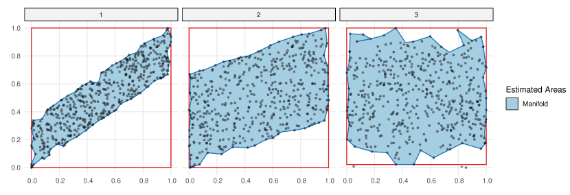
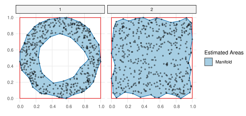
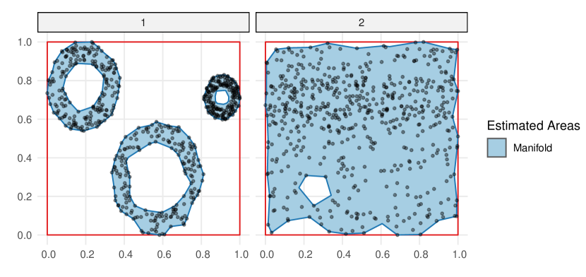
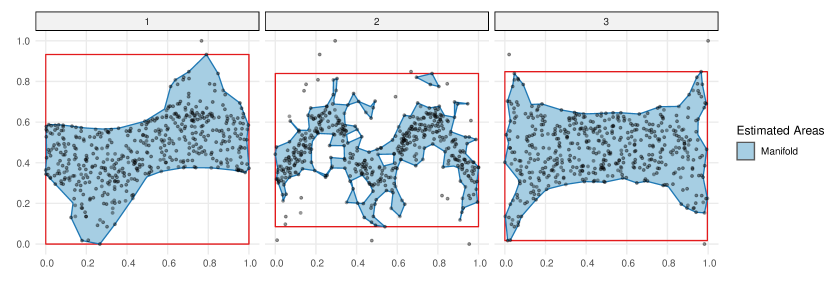
The figures presented in this section represent the estimated manifold for each input variable $X_{i}$ with respect to the output variable $Y$. The table below each figure presents the radius used to build the neighborhood graph, the estimated areas of the manifold object, of the reference square, and the proposed index.

The linear model in Figure 4 is simple enough to allow us to directly see that variable $X_{1}$ explains almost double the variability than variable $X_{2}$. Variables $X_{3}$ to $X_{5}$ will have less important indices. In this case, given the linearity, the normal $R^{2}$ score covers almost 81% of the variance for the $X_{1}$. The rest of the total variance is covered by $X_{2}$. The rest of variables have negligible scores. We observe how the empty spaces proliferate according to the relevance level of the variable.

The model of circle with one hole in Figure 5 was discussed in the preliminaries. Recall that in this case both variables have $R^{2}$ scores near zero for our model even if the geometric shape showed the contrary. Observe how the first variable has index equal to $0.46$ and the second one $0.07$. This allows us to say that the VR-complex built for $X_{1}$ performs better when explaining the data than just enclosing it in a square. For the second variable the VR-complex and the enclosed square perform similar, thus the geometric goodness-of-fit is almost zero.

To test our algorithm further we present the model of connected circles with holes in Figure 6. Here we created three circles with different scales and positions. We could capture the most relevant features for each projection. In this case the classic $R^{2}$ could capture only a mere 19% of the explained variance of the model for the first variable. For the second one the $R^{2}$ score is near to zero. Meanwhile, the $R^{2}_{\text{Geom}}$ score could detect almost 53% of correspondence between the first variable and the outcome. In this case, our method performs better at detecting the anomalous pattern.

The final model is produced by the Ishigami function, Figure 7. This is a popular model in sensitivity analysis because it presents a strong non-linearity and non-monotonicity with interactions in $X_{3}$. With other sensitivity estimators the variables $X_{1}$ and $X_{2}$ have great relevance to the model, while the third one $X_{3}$ has almost zero. For a further explanation of this function we refer the reader to Sobol1999 . The first, second and third variables explain 33%, 48% and 1% of the variance respectively. In particular, notice how the third variable is considered pure noise for the regression polynomial model. Also, notice how in this case, the $R^{2}_{\text{Geom}}$ scores for the three variables are around the 50% and 60%. It indicates, for the three variables, that a geometric pattern was revealed by the VR-complex. The three variables present large areas of blank spaces inside their boxes.

Variable	$\varepsilon$	$\mathrm{Area}(\mathcal{R}_{\varepsilon})$	$\mathrm{Area}(B)$	$R^{2}_{\mathrm{Geom}}$	$R^{2}$
$X_{1}$	0.08	0.31	1.00	0.69	0.81
$X_{2}$	0.12	0.64	1.00	0.36	0.19
$X_{3}$	0.15	0.80	0.98	0.19	0.01

Figure 4: Results for the linear case.

Variable	$\varepsilon$	$\mathrm{Area}(\mathcal{R}_{\varepsilon})$	$\mathrm{Area}(B)$	$R^{2}_{\mathrm{Geom}}$	$R^{2}$
$X_{1}$	0.15	0.50	1.00	0.50	0.01
$X_{2}$	0.14	0.90	1.00	0.10	0.01

Figure 5: Results for the circle with 1 hole case.

Variable	$\varepsilon$	$\mathrm{Area}(\mathcal{R}_{\varepsilon})$	$\mathrm{Area}(B)$	$R^{2}_{\mathrm{Geom}}$	$R^{2}$
$X_{1}$	0.09	0.24	1.00	0.76	0.67
$X_{2}$	0.16	0.90	1.00	0.10	0.01

Figure 6: Results for the circle with 2 holes case.

Variable	$\varepsilon$	$\mathrm{Area}(\mathcal{R}_{\varepsilon})$	$\mathrm{Area}(B)$	$R^{2}_{\mathrm{Geom}}$	$R^{2}$
$X_{1}$	0.16	0.41	0.93	0.56	0.33
$X_{2}$	0.08	0.23	0.75	0.69	0.48
$X_{3}$	0.12	0.41	0.83	0.50	0.01

Figure 7: Results for the Ishigami case.

4 Conclusions and further research

As mentioned above the aim of this paper was to build a goodness-of-fit index relying solely on the topological and geometrical features of a data-cloud. Purely analytic or statistical methods cannot recognize the structure when we project certain variables, primarily when the input is of zero-sum, which might be  artificial noise. In such cases those projections, or the variables in question, have positive conditional variance that might contribute to the model in ways that had not been explored.

Our index proved to be reliable in detecting  variability of the data when the variable is of zero-sum, differentiating between pure random noise and well-structured inputs. Where the model presents pure noise, our index coincides fully with other methods’ indexes. It also detects relevant structured inputs, in the other cases our index shows the structure in all the variables, which was the notion we wanted to explore.

We do not have yet an efficient and transparent index that measures the geometric goodness-of-fit through the VR-complex. To reach this point we identify a series of research problems to be dealt in the near future: Construct a better and faster to have the base graph. Alternatively, change it to make the process more efficient and hence allow ourselves to run more sophisticated examples, both theoretical and real data examples from controlled examples. One of the central points to be discussed and studied further is determining the radius of proximity, which we believe must be given by the data-set itself, probably by a more detailed application of persistent homology. Finally, we look forward to extending our method to more than one variable at a time, to cross-check relevance between variables.

Our major goal for a future project is to asses whether our model is useful in determining the relevance of a variable within a model.

Supplementary Material

R-package for TopSA routine:

R-package “TopSA” estimates sensitivity indices reconstructing the embedding manifold of the data. The reconstruction is done via a Vietoris Rips with a fixed radius. Then the homology of order 2 and the indices are estimated. https://github.com/maikol-solis/topsa

References

- (1) Hastie T, Tibshirani R, Friedman J. The Elements of Statistical Learning. vol. 1 of Springer Series in Statistics. New York, NY: Springer-Verlag New York; 2009.
- (2) Hand DJ. Pattern Recognition. In: Rao CR, Wegman EJ, Solka JL, editors. Handbook of Statistics. volumen 24 ed. Elsevier B.V; 2005. p. 213–228.
- (3) Tufte ER. The visual display of quantitative information. Graphics Press; 2001.
- (4) Myatt GJ, Johnson WP. Making Sense of Data II. Hoboken, NJ, USA: John Wiley & Sons, Inc.; 2009.
- (5) Buja A, Cook D, Asimov D, Hurley C. Computational Methods for High-Dimensional Rotations in Data Visualization; 2005. p. 391–413.
- (6) Barrett JP. The coefficient of determination-some limitations. American Statistician. 1974 feb;28(1):19–20.
- (7) Barten AP. Note on unbiased estimation of the squared multiple correlation coefficient. Statistica Neerlandica. 1962 jun;16(2):151–164.
- (8) Press SJ, Zellner A. Posterior distribution for the multiple correlation coefficient with fixed regressors. Journal of Econometrics. 1978 dec;8(3):307–321.
- (9) Cramer JS. Mean and variance of R2 in small and moderate samples. Journal of Econometrics. 1987 jul;35(2-3):253–266.
- (10) Tenenbaum JB. A Global Geometric Framework for Nonlinear Dimensionality Reduction. Science. 2000 dec;290(5500):2319–2323.
- (11) Bernstein M, de Silva V, Langford JC, Tenenbaum JB. Graph approximations to geodesics on embedded manifolds. Igarss 2014. 2000;01(1):1–5.
- (12) Balasubramanian M. The Isomap Algorithm and Topological Stability. Science. 2002 jan;295(5552):7a–7.
- (13) Ghrist R. Barcodes: The persistent topology of data. Bulletin of the American Mathematical Society. 2008 oct;45(1):61–75.
- (14) Carlsson G. Topology and data. Bulletin of the American Mathematical Society. 2009 jan;46(2):255–308.
- (15) Carlsson G. Topological pattern recognition for point cloud data. Acta Numerica. 2014 may;23(23):289–368.
- (16) Gallón S, Loubes JM, Maza E. Statistical properties of the quantile normalization method for density curve alignment. Mathematical Biosciences. 2013 apr;242(2):129–142.
- (17) Dimeglio C, Gallón S, Loubes JM, Maza E. A robust algorithm for template curve estimation based on manifold embedding. Computational Statistics and Data Analysis. 2014 feb;70:373–386.
- (18) Snášel V, Nowaková J, Xhafa F, Barolli L. Geometrical and topological approaches to Big Data. Future Generation Computer Systems. 2017 feb;67:286–296.
- (19) Bellman R. Dynamic Programming. Dover Books on Computer Science Series. Princeton University Press; 1957.
- (20) Bellman R. Adaptive control processes: A guided tour. vol. 4 of ’Rand Corporation. Research studies. Princeton University Press; 1961.
- (21) Hatcher A. Algebraic topology. Cambridge: Cambridge Univ. Press; 2000. Available from: https://cds.cern.ch/record/478079.
- (22) Munkres JR. Elements of Algebraic Topology. Addison-Wesley; 1984.
- (23) Zomorodian A, Carlsson G. Computing persistent homology. Proceedings of the twentieth annual symposium on Computational geometry - SCG ’04. 2005 feb;33(2):347. Available from: http://portal.acm.org/citation.cfm?doid=997817.997870http://link.springer.com/10.1007/s00454-004-1146-y.
- (24) Zomorodian A. Fast construction of the Vietoris-Rips complex. Computers & Graphics. 2010 jun;34(3):263–271.
- (25) de Silva V, Ghrist R. Coverage in sensor networks via persistent homology. Algebraic & Geometric Topology. 2007 apr;7(1):339–358. Available from: http://www.msp.org/agt/2007/7-1/p16.xhtml.
- (26) Eppstein D, Löffler M, Strash D. Listing All Maximal Cliques in Sparse Graphs in Near-Optimal Time. In: Lecture Notes in Computer Science (including subseries Lecture Notes in Artificial Intelligence and Lecture Notes in Bioinformatics). vol. 6506 LNCS; 2010. p. 403–414.
- (27) Bron C, Kerbosch J. Algorithm 457: finding all cliques of an undirected graph. Communications of the ACM. 1973;16(9):575–577.
- (28) Fasy BT, Kim J, Lecci F, Maria C, Millman DL, included GUDHI is authored by Clement Maria VRT, et al.. TDA: Statistical Tools for Topological Data Analysis; 2019. Available from: https://cran.r-project.org/package=TDA.
- (29) Pebesma E. Simple Features for R: Standardized Support for Spatial Vector Data. The R Journal. 2018;10(1):439. Available from: https://doi.org/10.32614/RJ-2018-009https://journal.r-project.org/archive/2018/RJ-2018-009/index.html.
- (30) Sobol’ IM, Levitan YL. On the use of variance reducing multipliers in Monte Carlo computations of a global sensitivity index. Computer Physics Communications. 1999 mar;117(1-2):52–61.