A Comparison of $p$-$g$ Tidal Coupling Analyses

Abstract

Two recent studies have attempted to constrain the proposed $p\text{-}g$ tidal instability with gravitational-wave data from GW170817. The studies use Bayesian methods to compare a model that includes $p\text{-}g$ tidal effects with one that does not. Using the same data, they arrive at very different conclusions. Reyes & Brown find that the observations of GW170817 strongly disfavor the existence of $p$-$g$ mode coupling. However, the LIGO and Virgo Collaborations find that neither model is strongly favored. We investigate the origin of this discrepancy by analyzing Reyes & Brown’s publicly available posterior samples. Contrary to their claims, we find that their samples do not disfavor $p\text{-}g$ mode coupling.

I Introduction

The gravitational wave (GW) observation of a coalescing binary neutron star (NS) system (GW170817 Abbott and etal (2017)) provides new insights into NS physics, including constraints on the high-density equation of state The LIGO Scientific Collaboration et al. (2018a); Abbott and et al. (2017) and tidal deformability De et al. (2018); The LIGO Scientific Collaboration et al. (2018b, a). Recently, two papers have attempted to constrain the $p\text{-}g$ tidal instability with GW170817 (Reyes and Brown (2018); The LIGO Scientific Collaboration et al. (2018c); hereafter RB and LVC, respectively). The instability involves a non-resonant coupling of the linear tidal bulge to high-frequency, pressure-supported modes ($p$-modes) and low-frequency, gravity-supported modes ($g$-modes) within the NS Weinberg et al. (2013); Venumadhav et al. (2014); Weinberg (2016); Zhou and Zhang (2017). Once unstable, the excited modes continuously drain energy from the orbit and accelerate the rate of GW-driven inspiral. The precise impact on the phasing of the GW signal is, however, unknown due to theoretical uncertainties in how the instability grows and saturates, although studies suggest that its impact might be observable with the current LIGO The LIGO Scientific Collaboration (2015) and Virgo et al (2015) interferometers Weinberg (2016); Essick et al. (2016).

RB and LVC attempt to constrain $p\text{-}g$ effects in GW170817 using the phenomenological model developed by Essick et al. (2016). Both studies employ a modification of the TaylorF2 frequency-domain waveform (see, e.g., Buonanno et al. (2009)) that includes an additional phase correction induced by $p\text{-}g$ effects. Using Bayesian methods, they compare models with $p\text{-}g$ effects ($\mathcal{H}_{pg}$) to models without $p\text{-}g$ effects ($\mathcal{H}_{!pg}$) and compute Bayes Factors $B^{pg}_{!pg}\equiv p(\mathrm{D}|\mathcal{H}_{pg})/p(\mathrm{D}|\mathcal{H}_{!pg})$, where $D$ refers to the data from GW170817.

While RB and LVC analyze the same data and use the same phenomenological $p\text{-}g$ waveform, there are differences in their models and priors, which we describe in Section II. Most notably, RB constructs an $\mathcal{H}_{pg}$ model that only includes “detectable $p\text{-}g$ effects” whereas LVC uses a wider $\mathcal{H}_{pg}$ model. RB finds that their models yield $B^{pg}_{!pg}<10^{-4}$ and LVC finds that their models yield $B^{pg}_{!pg}\approx 1$. Thus, RB concludes that the observations strongly disfavor their $\mathcal{H}_{pg}$ model and LVC concludes that the observations do not favor either of their models.

A priori, the disparate $B^{pg}_{!pg}$ could be due to differences in the studies’ models and priors. However, we show in Section III that this cannot be the explanation. We use the posterior samples from RB to compute $B^{pg}_{!pg}$ using LVC’s method for calculating Bayes Factors The LIGO Scientific Collaboration et al. (2018c). We find that LVC’s method applied to RB’s posterior samples, and thus their models and priors, yield $B^{pg}_{!pg}\approx 1$ and not $B^{pg}_{!pg}<10^{-4}$. This indicates that there is an error in how RB calculates $B^{pg}_{!pg}$. Our estimate implies that their $\mathcal{H}_{pg}$ model is not disfavored by the data.

II Comparison of Models and Priors

The phenomenological model presented in Essick et al. (2016) introduces three $p\text{-}g$ parameters per NS (indexed by $i\in\{1,2\}$): an overall amplitude ($A_{i}$) related to how many modes become unstable, how quickly they grow, and the energy at which they saturate; a turn-on/saturation frequency ($f_{i}$) that is related to when the modes first become unstable; and a spectral index ($n_{i}$) that describes how the rate of energy dissipation evolves with the orbital frequency (see Essick et al. (2016), RB, and LVC).

The frequency-domain phase shift $\Delta\Psi(f)$ induced by $p\text{-}g$ effects is given by Equation (3) in RB and Equation (1) in LVC. To account for a possible dependence on the component masses ($m_{i}$), Essick et al. (2016) introduces a Taylor expansion of the $p\text{-}g$ parameters around $m_{i}=1.4M_{\odot}$. LVC keeps the zeroth- and first-order coefficients of the expansion (their Equation (2)). RB keeps only the zeroth order coefficients. However, this should not introduce large discrepancies since LVC and Essick et al. (2016) find that the first order terms are not measurable.

In their Equation (3), RB neglects a dependence on the component masses that exists independent of the Taylor expansion. Specifically, in the expression for $\Delta\Psi(f)$, there is a factor $C_{i}=[2m_{i}/(m_{1}+m_{2})]^{2/3}A_{i}$ and RB assumes $C_{1}/A_{1}=C_{2}/A_{2}$ even when $m_{1}\neq m_{2}$. However, since the difference is small for reasonable ranges of $m_{i}$, this should not introduce a large discrepancy.

RB’s priors on the non-$p\text{-}g$ parameters are somewhat different from LVC’s. RB considers both a uniform and a Gaussian prior on $m_{i}$, whereas LVC considers only a uniform prior on $m_{i}$. While RB’s estimates of $B^{pg}_{!pg}$ vary by as much as a factor of $10^{3}$ for different mass priors, they note that their posterior distributions are qualitatively very similar. In addition, unlike LVC, RB assumes a fixed source location and distance based on the electromagnetic counterparts to GW170817 Abbott and et al (2017); Abbott and et al. (2017). However, Essick et al. (2016) found that extrinsic parameters do not strongly impact the inference of $p\text{-}g$ effects.

RB also assumes the NSs have equal radii and their priors on component spins differ from LVC’s. However, we do not believe this could introduce large discrepancies.

The differences between RB’s and LVC’s priors on the $p\text{-}g$ parameters are more substantial. The most significant difference is that LVC assumes uniform priors on the zeroth order coefficients $\log_{10}A_{0}$, $f_{0}$, and $n_{0}$ (following Essick et al. (2016)), whereas RB constrains the $p\text{-}g$ parameters to values that produce total time-domain phase shifts $\delta\phi\geq 0.1\,\mathrm{rad}$. Thus, RB’s priors on $\log_{10}A_{0}$, $f_{0}$, and $n_{0}$ are not uniform, but favor combinations that produce relatively large $p\text{-}g$ tidal effects. RB explains that for $m_{1}=m_{2}=1.4M_{\odot}$, there is a 99.98% overlap between the waveforms from $\mathcal{H}_{pg}$ and $\mathcal{H}_{!pg}$ for values of $(A_{0},f_{0},n_{0})$ that yield $\delta\phi\approx 0.1\textrm{ rad}$. As a result, like LVC, their prior still allows certain limits of $\mathcal{H}_{pg}$ to reproduce $\mathcal{H}_{!pg}$.

Finally, LVC focuses on a somewhat narrower bandwidth than RB (minimum frequencies of 30 Hz vs. 20 Hz). LVC does explore minimum frequencies above 30 Hz and find that $B^{pg}_{!pg}$ only varies by factors of order unity (see their Figure 1). Since the gain in signal-to-noise ratio from 30 Hz to 20 Hz is relatively modest ($\lesssim$ few percent), we do not believe this difference introduces large discrepancies.

III Comparison of results

Figure 1: Posteriors, priors and $B^{pg}_{!pg}$ computed using RB’s posterior samples showing disagreement with RB’s claim that $B^{pg}_{!pg}<10^{4}$. (top) Kernel density estimates of the marginal prior $\ln p(A_{0}|\mathcal{H}_{pg})$, (middle) marginal posterior $\ln p(A_{0}|\mathrm{data},\mathcal{H}_{pg})$, and (bottom) the associated $\ln B^{pg}_{!pg}$ using RB’s publicly available uniform-mass, small $f_{0}$ posterior samples. We evaluate these at several values of $\log_{10}A_{0}$. These distributions reflect the statistical uncertainty in the exact value of the priors, posteriors, and $\ln B^{pg}_{!pg}$ from the finite number of samples. By taking the difference between $\ln p(A_{0}|\mathcal{H}_{pg})$ and $\ln p(A_{0}|\mathrm{data},\mathcal{H}_{pg})$, we obtain the distributions for $\ln B^{pg}_{!pg}$.

In order to compute Bayes Factors, RB uses thermodynamic integration Lartillot and Philippe (2006); Foreman-Mackey et al. (2013); Vousden et al. (2016); Wang and Swendsen (2005); Earl and Deem (2005); Biwer et al. (2018) while LVC uses the Savage-Dickey Density Ratio (SDDR, see Dickey and Lientz (1970); Verdinelli and Wasserman (1995); Wagenmakers et al. (2010) and Appendix A). In principle, both should yield consistent results. However, when we apply the SDDR to RB’s (uniform-mass, small $f_{0}$) posterior samples, we find $\ln B^{pg}_{!pg}\approx+0.7$ whereas RB claims $\ln B^{pg}_{!pg}=-21$ ($\log_{10}B^{pg}_{!pg}=-9.2$) for the same posterior samples.

The SDDR provides a convenient way to estimate Bayes Factors between nested models when the posterior is available for the larger model. In the limit of small $A_{0}$ (see LVC’s Equation (3) and Appendix A),

$$\lim\limits_{A_{0}\rightarrow 0}\frac{p(A_{0}|\mathrm{data},\mathcal{H}_{pg})}{p(A_{0}|\mathcal{H}_{pg})}\simeq\frac{p(\mathrm{data}|\mathcal{H}_{!pg})}{p(\mathrm{data}|\mathcal{H}_{pg})}=\frac{1}{B^{pg}_{!pg}}.$$ (1)

This says that $B^{pg}_{!pg}$ equals the ratio of the marginal distribution of $A_{0}$ a priori to the marginal distribution of $A_{0}$ a posteriori provided that both are evaluated at small $A_{0}$. Intuitively, if at some small $A_{0}$ the probability density is small a priori but large a posteriori, then the data must favor small $A_{0}$ and $B^{pg}_{!pg}$ should be small (and vice versa).

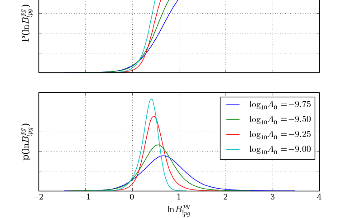
RB finds $B^{pg}_{!pg}<10^{-4}$, which implies that, at small $A_{0}$, their prior density is $>10^{4}$ times smaller than their posterior density. However, Figures 1–3 in RB show that their prior and posterior densities are similar at small $A_{0}$, which instead suggests $B^{pg}_{!pg}\approx 1$. More precisely, we find that the SDDR yields $B^{pg}_{!pg}\simeq+2.0$ for RB’s uniform-mass, small $f_{0}$ prior and similar $B^{pg}_{!pg}$ for their other priors. Since $B^{pg}_{!pg}>1$, formally RB’s results actually slightly favor the existence of detectable $p\text{-}g$ effects. However, the preference is not large enough to be significant (see the calculation of the False Alarm Probability in LVC).

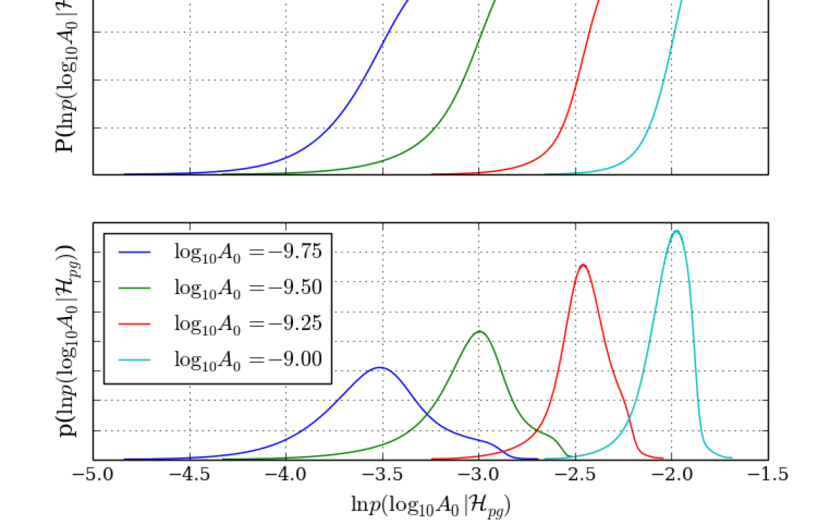
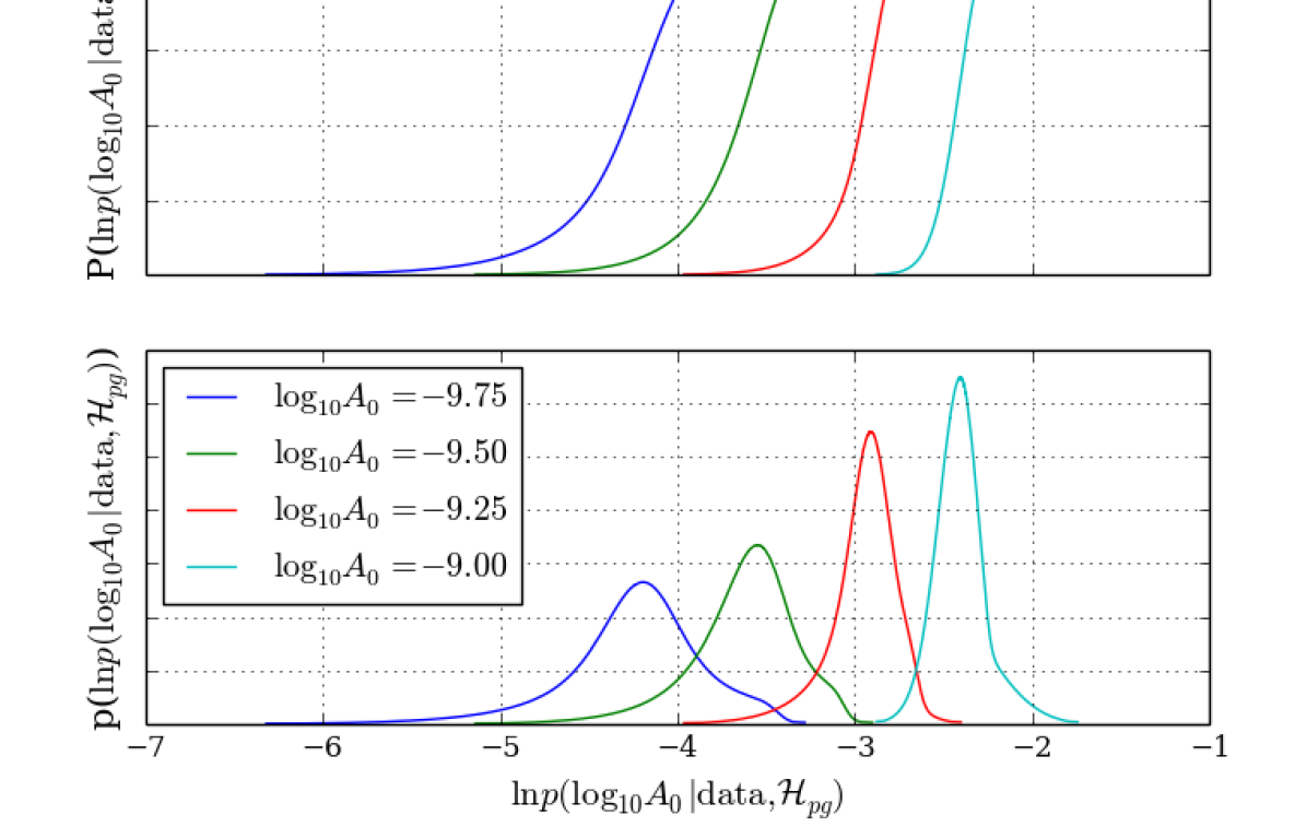
We show this result in more detail in Figure 1. Using RB’s samples, we plot the probability densities of the priors, posteriors, and their ratio (i.e., $B^{pg}_{!pg}$) at several values of small $A_{0}$. Because closed-form expressions for the priors and posteriors are not available, we estimate these from RB’s public samples. There are only a finite number of samples available, and the distributions in Figure 1 show the uncertainty in our estimates of the prior and posterior at a few values of $\log_{10}A_{0}$. These figures were generated using the same code LVC used to estimate $\ln B^{pg}_{!pg}$in their Figure 1. For brevity, we focus on RB’s uniform-mass, small $f_{0}$ range posteriors (their Figure 2) but find similar results for their other data. Although the posteriors and priors are not constant as $A_{0}\rightarrow 0$, what is important is that their ratio, and hence $B^{pg}_{!pg}$, are consistently $\mathcal{O}(1)$.

IV Examination of RB’s Implementation of Thermodynamic Integration

To investigate RB’s systematic error further, we attempt to repeat their calculation using thermodynamic integration. Thermodynamic integration makes use of the convenient identity for the evidence $Z_{\mathcal{H}}=p(d|\mathcal{H})$

$$\frac{d}{d\beta}\ln Z_{\mathcal{H}}(\beta) =\frac{d}{d\beta}\ln\int d\theta\,p(d|\theta)^{\beta}p(\theta|\mathcal{H})$$

$$=\frac{\int d\theta\left(\ln p(d|\theta)\right)p(d|\theta)^{\beta}p(\theta|\mathcal{H})}{\int d\theta\,p(d|\theta)^{\beta}p(\theta|\mathcal{H})}$$

$$=\left<\ln p(d|\theta)\right>_{p_{\beta}(\theta|d;\mathrm{H})}$$ (2)

By running several parallel Markov-Chain Monte Carlo instances, each at a different temperature $T=1/\beta$, one can approximate $d\ln Z/d\beta$ as a function of $\beta$ by computing the average of $\ln p(d|\theta)$ with respect to $p_{\beta}(\theta|d;\mathcal{H})\propto p(d|\theta)^{\beta}p(\theta|\mathcal{H})$. With enough temperatures, an estimate for the evidence is obtained as

$$\ln Z_{\mathcal{H}}=\int\limits_{0}^{1}d\beta\frac{d}{d\beta}\ln Z_{\mathcal{H}}=\int\limits_{0}^{1}d\beta\left<\ln p(d|\theta)\right>_{p_{\beta}(\theta|d;\mathrm{H})}$$ (3)

Typically, the set of temperatures is chosen to optimize sampling through parallel tempering (see, e.g., Vousden et al. (2016); Earl and Deem (2005)) and the resulting integral is estimated via a trapazoidal approximation. This procedure is repeated for each model separately, and then differences in the evidences yield Bayes Factors.

RB attempt to implement this approach. However, as shown by their public data, they only use 3 temperatures, and the smallest inverse temperature used is $\beta\simeq 0.25$. When checking our implementation of the Savage-Dickey Density Ratio against thermodynamic integration on our own data, we only found convergence with at least 12 temperatures. This means that not only do they poorly resolve the numeric integral, they severely truncate the estimate. Therefore, the RB result contains large systematic errors.

RB rely upon evidence estimates from previous work De et al. (2018) when estimating Bayes Factors. Examination of the public data from De et al. (2018) shows that they also used only 3 temperatures and incorrectly truncated the integral. The Bayes factors originally quoted in De et al. (2018) are therefore also in error (as the erratum in De et al. (2018) acknowledges).

V Conclusions

We analyzed the publicly available samples from Reyes & Brown Reyes and Brown (2018). Using our own method for calculating Bayes Factors The LIGO Scientific Collaboration et al. (2018c), we find that their samples yield $B^{pg}_{!pg}\simeq+2.0$ and not $B^{pg}_{!pg}<10^{-4}$. The source of their errors stems from a flawed implementation of thermodynamic integration, which also affected some of the authors’ other work (see erratum in De et al. (2018)). We therefore conclude that, contrary to Reyes & Brown’s claim, their posterior data do not disfavor $p\text{-}g$ mode coupling.

Appendix A Derivation of the Savage-Dickey Density Ratio

According to Bayes theorem

$$p(A_{0},f_{0},n_{0},\theta|D;\mathcal{H}_{pg})=\frac{1}{p(D|\mathcal{H}_{pg})}p(D|A_{0},f_{0},n_{0},\theta;\mathcal{H}_{pg})p(A_{0},f_{0},n_{0},\theta|\mathcal{H}_{pg}),$$ (4)

where $\theta$ refers to all parameters besides the $p\text{-}g$ parameters and $D$ to the data from GW170817. We drop the first-order terms in the $p\text{-}g$ parameter Taylor expansions for clarity, but they could be included in a straightforward way. The marginal posterior distribution for $A_{0}$ is therefore

$$p(A_{0}|D;\mathcal{H}_{pg}) =\frac{1}{p(D|\mathcal{H}_{pg})}\int d\theta df_{0}dn_{0}p(D|A_{0},f_{0},n_{0},\theta;\mathcal{H}_{pg})p(A_{0},f_{0},n_{0},\theta|\mathcal{H}_{pg})$$

$$=\frac{1}{p(D|\mathcal{H}_{pg})}\int d\theta df_{0}dn_{0}p(D|A_{0},f_{0},n_{0},\theta;\mathcal{H}_{pg})p(f_{0},n_{0}|A_{0},\theta;\mathcal{H}_{pg})p(\theta|A_{0};\mathcal{H}_{pg})p(A_{0}|\mathcal{H}_{pg}).$$ (5)

Although $\mathcal{H}_{!pg}$ is not formally contained in $\mathcal{H}_{pg}$ for uniform-in-$\log_{10}A_{0}$ priors, the lower limit of $A_{0}=10^{-10}$ (in both studies) is sufficiently small that $\mathcal{H}_{!pg}$ is, to a very good approximation, nested in $\mathcal{H}_{pg}$. In particular, at $A_{0}=10^{-10}$, the waveforms of $\mathcal{H}_{pg}$  and $\mathcal{H}_{!pg}$ match to $>99.999\%$. Therefore, in the limit $A_{0}\rightarrow 10^{-10}$, the likelihood $p(D|A_{0},f_{0},n_{0},\theta;\mathcal{H}_{pg})=p(D|\theta;\mathcal{H}_{!pg})$ and the integral factors. We then have

$$\lim\limits_{A_{0}\rightarrow 10^{-10}}\frac{p(A_{0}|D;\mathcal{H}_{pg})}{p(A_{0}|\mathcal{H}_{pg})} =\frac{1}{p(D|\mathcal{H}_{pg})}\lim\limits_{A_{0}\rightarrow 10^{-10}}\int d\theta df_{0}dn_{0}p(D|A_{0},f_{0},n_{0},\theta;\mathcal{H}_{pg})p(f_{0},n_{0}|A_{0},\theta,\mathcal{H}_{pg})p(\theta|A_{0};\mathcal{H}_{pg})$$

$$=\frac{1}{p(D|\mathcal{H}_{pg})}\lim\limits_{A_{0}\rightarrow 10^{-10}}\left(\int d\theta p(D|\theta;\mathcal{H}_{!pg})p(\theta|A_{0};\mathcal{H}_{pg})\right.$$

$$\left.\quad\quad\quad\quad\quad\quad\quad\quad\quad\quad\quad\quad\quad\quad\quad\quad\quad\quad\quad\quad\times\left[\int df_{0}dn_{0}p(f_{0},n_{0}|\theta,A_{0};\mathcal{H}_{pg})\right]\right).$$ (6)

This allows us to integrate away the conditional prior for $f_{0}$ and $n_{0}$ and obtain

$$\lim\limits_{A_{0}\rightarrow 10^{-10}}\frac{p(A_{0}|D;\mathcal{H}_{pg})}{p(A_{0}|\mathcal{H}_{pg})} =\frac{1}{p(D|\mathcal{H}_{pg})}\lim\limits_{A_{0}\rightarrow 10^{-10}}\int d\theta p(D|\theta;\mathcal{H}_{!pg})p(\theta|\mathcal{H}_{!pg})\left[\frac{p(\theta|A_{0};\mathcal{H}_{pg})}{p(\theta|\mathcal{H}_{!pg})}\right]$$

$$=\frac{p(D|\mathcal{H}_{!pg})}{p(D|\mathcal{H}_{pg})}\lim\limits_{A_{0}\rightarrow 10^{-10}}\left(\int d\theta p(\theta|D;\mathcal{H}_{!pg})\frac{p(\theta|A_{0};\mathcal{H}_{pg})}{p(\theta|\mathcal{H}_{!pg})}\right).$$ (7)

Thus

$$\lim\limits_{A_{0}\rightarrow 10^{-10}}\frac{p(A_{0}|D;\mathcal{H}_{pg})}{p(A_{0}|\mathcal{H}_{pg})}=\frac{1}{B^{pg}_{!pg}}\lim\limits_{A_{0}\rightarrow 10^{-10}}\left<\frac{p(\theta|A_{0};\mathcal{H}_{pg})}{p(\theta|\mathcal{H}_{!pg})}\right>_{p(\theta|D;\mathcal{H}_{!pg})},$$ (8)

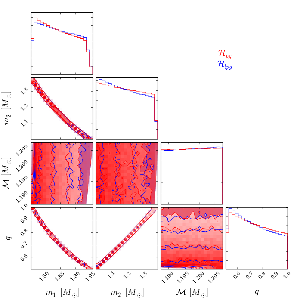
where $\left<x\right>_{p}$ denotes the average of $x$ with respect to the measure defined by $p$. As we demonstrate in Figure 2, $\lim_{A_{0}\rightarrow 10^{-10}}p(\theta|A_{0};\mathcal{H}_{pg})\approx p(\theta|\mathcal{H}_{!pg})$. The red curves show the conditional prior distributions for component masses ($m_{1}$, $m_{2}$), chirp mass ($\mathcal{M}$), and mass ratio ($q=m_{2}/m_{1}\leq 1$) under RB’s $\mathcal{H}_{pg}$ priors for $\log_{10}A_{0}\in[-10,-9.9]$. The blue curves show the distributions for an analogous prior with uniform distributions for $m_{1}$ and $m_{2}$ and the same $\mathcal{M}$ cuts but without any requirement on $\delta\phi$, which is RB’s corresponding $\mathcal{H}_{!pg}$ prior. While we see some small differences in the marginal distributions, these are all $\mathcal{O}(1)$. We therefore expect $\left<p(\theta|A_{0};\mathcal{H}_{pg})/p(\theta|\mathcal{H}_{!pg})\right>_{p(\theta|\mathcal{H}_{!pg})}$ to be a negligible correction and omit it from the main body of this note (Equation (1)). Therefore, the ratio of the marginal posterior to the marginal prior, when evaluated at sufficiently small $A_{0}$, yields an accurate an estimate of $B^{pg}_{!pg}$.

Figure 2: Mass priors in RB’s analysis, which enter as a correction factor in Equation (8). (red) $p(\theta|A_{0};\mathcal{H}_{pg})$ with $\log_{10}A_{0}\in[-10,-9.9]$. (blue) $p(\theta|\mathcal{H}_{!pg})$ assuming uniform priors on component masses and the same $\mathcal{M}$ cuts RB uses for $\mathcal{H}_{pg}$.