Maximum Entropy Principle Analysis in Network Systems with Short-time Recordings

Abstract

In many realistic systems, maximum entropy principle (MEP) analysis provides an effective characterization of the probability distribution of network states. However, to implement the MEP analysis, a sufficiently long-time data recording in general is often required, e.g., hours of spiking recordings of neurons in neuronal networks. The issue of whether the MEP analysis can be successfully applied to network systems with data from short recordings has yet to be fully addressed. In this work, we investigate relationships underlying the probability distributions, moments, and effective interactions in the MEP analysis and then show that, with short recordings of network dynamics, the MEP analysis can be applied to reconstructing probability distributions of network states under the condition of asynchronous activity of nodes in the network. Using spike trains obtained from both Hodgkin-Huxley neuronal networks and electrophysiological experiments, we verify our results and demonstrate that MEP analysis provides a tool to investigate the neuronal population coding properties, even for short recordings.

PACS numbers

89.70.Cf, 87.19.lo, 87.19.ls, 87.19.ll

Introduction

Binary-state models have been used to describe the activity of nodes in many network systems, such as neuronal networks in neuroscience schneidman2006weak ; shlens2006structure ; xu2016dynamical . Understanding the distribution of network binary-state dynamics is important in unveiling underlying network function, especially in neuroscience where both theoretical and experimental results indicate that populations of neurons perform computations probabilistically through their firing patterns knill2004bayesian ; karlsson2009awake . For instance, statistical distributions of neuronal network firing patterns have been shown to perform awake replays of remote experiences in rat hippocampus karlsson2009awake . Therefore, studying the characteristics of neuronal firing pattern distributions will help to understand how neuronal networks encode information morcos2016history . However, this is a difficult task, since the number of all possible network states grows exponentially as the network size increases, i.e., $2^{n}$ for a network of $n$ binary-state nodes. This high dimensionality presents a challenge in directly measuring the distribution of network states in electrophysiological experiments, especially for the case of in vivo measurements on awake animals, thus, the difficulty in understanding coding schemes in neuronal networks.

The maximum entropy principle (MEP) analysis is a statistical method used to infer the least biased probability distribution of network states by maximizing the Shannon entropy with given constraints, i.e., moments up to certain order jaynes1957information . The inferred probability distribution is called the MEP distribution. For example, under constraints of low-order moments, the MEP distribution gives rise to an accurate estimate of the statistical distribution of network states in many scientific fields, e.g., neuroscience schneidman2006weak ; shlens2006structure ; tang2008maximum ; xu2016dynamical , biology sakakibara2009protein ; sulkowska2012genomics ; mantsyzov2014maximum , imaging science saremi2013hierarchical , economics golan1996maximum ; squartini2013early , linguistics stephens2010statistical , anthropology hernando2013workings , and atmosphere-ocean science khatiwala2009reconstruction .

However, a practical and important issue remains unclear: how well the MEP analysis performs when the recording time of dynamics of network nodes is short. This is because a very long recording is often required to carry out the MEP analysis, e.g., hours for a network of $10$ neurons schneidman2006weak . These long recordings are usually impractical to achieve due to cost or capability. For example, physiological constraints such as fatigue of neurons makes it very difficult to record the state of neuronal networks over a long time, especially in vivo recordings on awake animals. Meanwhile, data obtained by short recordings poorly captures many activity states, leading to incorrect descriptions for the probability distribution of network states. The insufficient measurements due to short recordings could lead to a misunderstanding of information coding structure embedded in network activity states ohiorhenuan2010sparse . Therefore, it is important to estimate an accurate probability distribution of network states from short recordings where many network activities are underrepresented.

In this work, we demonstrate that the MEP analysis can give rise to an accurate estimate of the probability distribution of network states from a short-time data recording if the activity of nodes in the network is asynchronous (asynchronous network). To achieve this, we first show the existence of a one-to-one mapping (denoted as the full-rank matrix ${\bf U}_{{\rm PM}}^{(n)}$ for a network of size $n$) between the probability distribution of network states (denoted by a vector of size $2^{n}$, $\mathbf{P}^{(n)}$) and the corresponding all moments (denoted by a vector of size $2^{n}$, $\mathbf{M}^{(n)}$). Since the full-order MEP distribution (the distribution obtained in the MEP analysis with constraints of all moments $\mathbf{M}^{(n)}$) and the probability distribution $\mathbf{P}^{(n)}$ are the same (they have all the same moments $\mathbf{M}^{(n)}$), we derive another one-to-one mapping (denoted as the full-rank matrix ${\bf L}_{{\rm JP}}^{(n)}$ for a network of size $n$) between all effective interactions (Lagrange multipliers corresponding to constraints of all moments in the expression of the full-order MEP distribution) and the probability distribution $\mathbf{P}^{(n)}$. These mappings show that all moments and all effective interactions can equivalently represent a probability distribution of network states for a general network of any size.

Next, we use the above equivalent representations to show that, in an asynchronous network, low-order MEP analysis gives rise to an accurate estimate of the probability distribution of network states from a short-time recording. In an asynchronous network, the probability of many nodes being active in one sampling time window (referred to as highly-active states) is very small. Through the mapping from effective interactions to the probability distribution, ${\bf L}_{{\rm JP}}^{(n)}$, we observe that the probability of a highly-active state can be written as a summation of effective interactions corresponding to the constraints of moments of those active nodes. In an asynchronous network, high-order effective interactions (Lagrange multipliers corresponding to the constraints of high-order moments) are usually small shlens2006structure ; schneidman2006weak ; tang2008maximum ; cavagna2014dynamical ; watanabe2013pairwise , as compared to the low-order effective interactions (Lagrange multipliers corresponding to the constraints of low-order moments). Then, the probabilities of highly-active states can be well estimated by the dominating low-order effective interactions. The MEP analysis shows that low-order effective interactions can be estimated by low-order moments through a widely-used iterative scaling algorithm (see Appendix A for details). Therefore, the low-order moments may possibly be measured accurately using short recording (as discussed below), and may be used to perform the MEP analysis to obtain a good estimate of the probability distribution of network states.

To obtain an accurate estimation of the low-order moments, we use properties of the mapping between the probability distribution of network states and the corresponding moments of the network, ${\bf U}_{{\rm PM}}^{(n)}$. This mapping shows that low-order moments can be written as a summation of all probability states in which those nodes corresponding to the constraints of moments are active, e.g., the first-order moment of node $i$ is a summation of all network-state probabilities in which node $i$ is active. This summation includes both highly-active state probabilities and low-active state probabilities in which few nodes are active in one sampling time window. Since the probability of observing a highly-active state is small in an asynchronous network, the low-active state probabilities dominate the summation. This results in good estimation for the low-order moments because low-active state probabilities can still be well-measured in a short recording and the noise for the estimation of low-order moments can be further reduced by the summation of low-active state probabilities saulis2012limit .

Although the procedure described in this work can be applied to any asynchronous network with binary dynamics, here we use spike trains obtained from both Hodgkin-Huxley (HH) neuronal network dynamics simulations and electrophysiological experiments to demonstrate that one can perform the MEP analysis to accurately estimate the probability distribution of network states from short-time recordings. For the case of simulation data from HH neuronal networks, we evolve the HH neuronal network for a short run time of $120\,\mathrm{s}$. With constraints of the first-order and the second-order moments of the data from this short recording, we obtain the distribution of network states from the MEP analysis. To verify the accuracy of the MEP distribution, we evolve the HH neuronal network for a long run time of $1.2\times 10^{5}\,\mathrm{s}$ and directly measure the probability distribution of network states for comparison. For the case of experimental data from electrophysiological measurements, we use data recorded from primary visual cortex (V1) in anesthetized macaque monkeys (See Appendix E for details), in which we use the data of $3824\,\mathrm{s}$ as a long recording data to obtain the probability distribution of network states and perform the second-order MEP analysis on the short-recording data of $191.2\,\mathrm{s}$ ($5\%$ of the total recording). Our results show that in both numerical simulation data and electrophysiological experimental data, these two distributions, i.e., the second-order MEP distribution and the distribution measured in the long recording data, indeed agree very well with each other, whereas the probability distribution measured from the short recording deviates significantly from them and cannot capture many neuronal activity states.

Methods: The MEP analysis

In this section, we will introduce the MEP analysis, which has been applied to estimating the probability distribution of network states for many network systems schneidman2006weak ; shlens2006structure ; tang2008maximum ; bury2012statistical ; cavagna2014dynamical . The process of performing the MEP analysis is as follows. Let $\sigma\in\{0,1\}$ denotes the state of a node in a sampling time bin, where 1 refers to an active state and 0 an inactive state. Then, the state of a network of $n$ nodes in a sampling time bin is denoted as $\Omega=(\sigma_{1},\sigma_{2},\cdots,\sigma_{n})\in\{0,1\}^{n}$. In principle, to obtain the probability distribution of $\Omega$, one has to measure all possible states of $\Omega$, i.e., $2^{n}$ states in total. For the case of a network of $n$ neurons, $\sigma$ often represents whether a single neuron fires in a sampling time bin in the network, where $1$ corresponds to a neuron that is firing and $0$ corresponds to a neuron in the silent state. We choose a typical bin size of $10\,\mathrm{ms}$ for the MEP analysis shlens2006structure ; tang2008maximum . The state, $\Omega$, in the neuronal network would represent the firing pattern of all neurons in the network.

The first-order moment of the state of node $i$, $\sigma_{i}$, is given by

$$\left\langle\sigma_{i}\right\rangle=\sum_{\Omega}P(\Omega)\sigma_{i}(\text{$\Omega)$},$$ (1)

where $P(\Omega)$ is the probability of observing the firing pattern $\Omega$ in the recording, and $\sigma_{i}(\text{$\Omega)$}$ denotes the state of the $i$th node in the firing pattern $\Omega$. The second-order moment of the state of node $i$, $\sigma_{i}$, and node $j$, $\sigma_{j}$, is given by

$$\left\langle\sigma_{i}\sigma_{j}\right\rangle=\sum_{\Omega}P(\Omega)\sigma_{i}(\text{$\Omega)$}\sigma_{j}(\text{$\Omega)$, }$$ (2)

with higher-order moments obtained similarly. Note that, in Eqs. (1, 2), $P(\Omega)$ can be the true probability distribution of $\Omega$, in which case, one computes the true moments; or $P(\Omega)$ can be an observed distribution of a finite-time recording, in which case, one then estimates the moments.

The Shannon entropy of a probability distribution $P_{{\rm any}}(\Omega)$ is defined as

$$S=-\sum_{\Omega}P_{{\rm any}}(\Omega)\log P_{{\rm any}}(\Omega).$$ (3)

By maximizing this entropy, $S$, subject to all moments up to the $m$th-order ($m\leq n$), one obtains the $m$th-order MEP distribution for a network of $n$ nodes schneidman2006weak ; shlens2006structure ; tang2008maximum . Note that the $k$th-order moments consist of all the expectations of the product of any $k$ nodes’ states (e.g., the second-order moments by Eq. (2) above for any pair of $i$ and $j$ with $i\neq j$) and thus when considering the constraint of the $k$th-order moments, there are $C_{n}^{k}$ (the number of combinations of $k$ nodes from $n$ possible choices) number of constraints of $k$th-order moments being considered. Finally, the $m$th-order probability distribution is obtained from the following equation,

$$P_{m}(\Omega)=\frac{1}{Z}\exp\left(\sum_{k=1}^{m}\sum_{i_{1}<\cdots<i_{k}}^{n}J_{i_{1}\cdots i_{k}}\sigma_{i_{1}}\cdots\sigma_{i_{k}}\right),$$ (4)

where, following the terminology of statistical physics, $J_{i_{1}\cdots i_{k}}$ is called the $k$th-order effective interaction ($2\leq k\leq m$), i.e., the Lagrange multiplier corresponding to the constraint of the $k$th-order moment $\left\langle\sigma_{i_{1}}\cdots\sigma_{i_{k}}\right\rangle$, and the partition function, $Z$, is a normalization factor. Eq. (4) is referred to as the $m$th-order MEP distribution. In practice, one can utilize an iterative scaling algorithm (see Appendix A for details) to numerically solve the above MEP optimization problem to obtain the effective interactions and thus the probability distribution in Eq. (4). Here, for a network of size $n$, $P_{n}(\Omega)$ is referred to as the full-order MEP distribution subject to moments of all orders.

Results

The results are organized as follows. We begin by demonstrating that there is a wide range of dynamical regimes where the neuronal network dynamics is asynchronous. Then, we show that the probability distribution of network states measured from a short-time recording (data recorded from the HH network dynamics with short simulation time) cannot capture many network activity states, and thus differs from the probability distribution of network states measured from a long-time recording. Note that we have verified that the HH network dynamics in a long simulation time of $1.2\times 10^{5}\,\mathrm{s}$ reaches the steady state; therefore, the probability distribution of network states measured from this long recording can well represent the true probability distribution of network states.

We next show that there exists a one-to-one mapping between the probability distribution of network states and the corresponding moments of the network. Then, we combine this mapping with the full-order MEP distribution to show that there exists a one-to-one mapping between all effective interactions and the probability distribution of network states. Using these mappings, we further demonstrate that high-order effective interactions are small in asynchronous networks; thus, to accurately estimate the probability distribution of network states, one may only require accurate estimation of the low-order effective interactions. Finally, we make use of low-order moments measured in short-time recordings to estimate low-order effective interactions and show that the obtained probability distribution from the low-order MEP analysis agrees well with the probability distribution of network states. This is demonstrated by both numerical simulations of asynchronous HH neuronal network dynamics and also electrophysiological experiments.

Short-time recordings cannot represent all network states

In this section, we first use numerical simulation data from the HH neuronal network dynamics and show that short-time recordings are often insufficient to accurately estimate the probability distribution of network states. Later, we will also demonstrate this issue using experimental data from electrophysiological measurements.

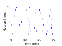
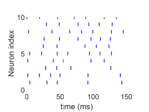
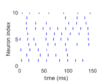
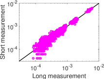
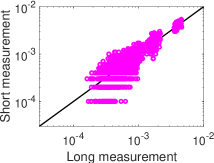
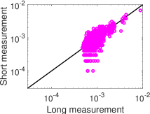
We simulate a network of $80$ excitatory and $20$ inhibitory HH neurons, with a $20\%$ connection density among neurons in the network. As physiological experiments can often only measure a subset of neurons, we randomly select $10\%$ of the neurons in the network ($10$ neurons) and demonstrate differences in the directly measured probability distribution between the short and the long recording. Note that there are typically three dynamical regimes for neuronal networks zhou2014granger : (i) a highly fluctuating regime where the input rate, $\mu$, is low (Fig. 1a); (ii) an intermediate regime where $\mu$ is moderately high (Fig. 1b); (iii) a low fluctuating or mean-driven regime where $\mu$ is very high (Fig. 1c). We evolve the HH neuronal network dynamics and record the spike trains of all neurons for a duration of $1.2\times 10^{5}\,\mathrm{s}$, which is sufficiently long to obtain a stable probability distribution of neuronal firing patterns. We then compare the probability distribution of network states directly measured in the short recording of $120\,\mathrm{s}$ to that measured in the long recording. As shown in Fig. 2, the measured probability distribution of firing patterns in the short recording deviates substantially from that in the long recording, for all three dynamical regimes.

The probability distribution of network states is important for a complete understanding of the underlying function of networks knill2004bayesian ; karlsson2009awake despite the fact that a sufficient long-time data recording is often impossible or impractical. Thus, it is essential to obtain an accurate estimate of the probability distribution of network states from a short-time recording. To achieve this, we next study relationships among the probability distribution, the moments, and the effective interactions in the MEP distribution and show that, for asynchronous networks, the second-order MEP analysis gives rise to an accurate estimate of the probability distribution of network states.

(a)

(b)

(c)

Figure 1: Raster plots for the HH neuronal network in three different dynamical regimes. Raster plots of $10$ randomly selected neurons for each case are shown. A short bar indicates that the neuron with certain index fires at certain time. The coupling strength is selected at random from the uniform distribution of the interval $[0,s]$, where $s=0.071\,\mathrm{ms^{-1}}$ (the corresponding physiological excitatory postsynaptic potential is $\sim 1\,\mathrm{mV}$). The Poisson input parameters for in (a), (b), and (c) are $(\mu=0.6\,\mathrm{ms^{-1}},\,f=0.05\,\mathrm{ms^{-1}})$, $(\mu=1.1\,\mathrm{ms^{-1}},\,f=0.04\,\mathrm{ms^{-1}})$ and $(\mu=2.5\,\mathrm{ms^{-1}},\,f=0.03\,\mathrm{ms^{-1}})$, respectively.

(a)

(b)

(c)

Figure 2: Measured probability distributions for short-time recordings compared with long-time recordings. The frequency of each firing state measured from the short-time recording of network dynamics ($120\,\mathrm{s}$) is plotted against the frequency measured from the long-time recording of network dynamics ($1.2\times 10^{5}\,\mathrm{s}$). Data for these three cases are from three dynamical regimes shown (the same $10$ selected neurons in each case) in Fig. 1, respectively.

One-to-one mapping between the probability distribution and the moments

To demonstrate the relationship between the true probability distribution of network states, $P_{{\rm true}}(\Omega)$, and the corresponding moments, we introduce several notations for ease of discussion. First, denote the vector $\mathbf{P}^{(n)}=(p_{1}^{(n)},p_{2}^{(n)},\cdots,p_{2^{n}}^{(n)})^{T}$ as the vector containing the probability distribution of the network states for a network of $n$ nodes, and denote the vector $\mathbf{M}^{(n)}=(m_{1}^{(n)},m_{2}^{(n)},\cdots,m_{2^{n}}^{(n)})^{T}$ as the vector containing all moments of the network. We arrange the entries in $\mathbf{P}^{(n)}$ and $\mathbf{M}^{(n)}$ as follows. For an example network of size $n=2$, we assign values to the $i$th entry by expressing $i-1$ using the base-2 number system with total $n=2$ digits, i.e., $E_{i}=e_{2}e_{1}$, where $E_{i}$ represents the combined state of the two nodes in the network, $e_{1}$ and $e_{2}$ (e.g., 00 corresponds to both nodes being inactive), as shown in the second column of Table 1. Then, for each $i$, denote the probability of the network state ($\sigma_{1}=e_{1},\sigma_{2}=e_{2})$ as $p_{i}^{(2)}$, as shown in the third column of Table 1. In neuroscience, the vector $P_{00}$ represents the probability of finding both two neurons in the quiet state, $P_{10}$ ($P_{01}$) represents the probability of the first (second) neuron in the active state and the second (first) neuron in the silent state, and $P_{11}$ represents the probability of both neurons in the active state. The entries in the vector $\mathbf{M}^{(2)}$ are arranged similarly, i.e., $m_{i}^{(2)}$ is the expectation of $(\sigma_{1})^{e_{1}}(\sigma_{2})^{e_{2}}$, as shown in the fourth column of Table 1.

i	$E_{i}=e_{2}e_{1}$	$p_{i}^{(2)}$	$m_{i}^{(2)}$
1	00	$P_{00}$	1
2	01	$P_{10}$	$\left\langle\sigma_{1}\right\rangle$
3	10	$P_{01}$	$\left\langle\sigma_{2}\right\rangle$
4	11	$P_{11}$	$\left\langle\sigma_{1}\sigma_{2}\right\rangle$

Table 1: Table of entries for building the vectors $\mathbf{P}^{(n)}$ and $\mathbf{M}^{(n)}$ for an example network of $n=2$ nodes.

For illustration, we show that, for a network of $n=2$ nodes, there is a full-rank matrix, $\mathbf{U}_{{\rm PM}}^{(2)}$, that transforms from the probability distribution to moments. From Eqs. (1) and (2), the expectation of $\sigma_{1}$, $\sigma_{2}$, and $\sigma_{1}\sigma_{2}$ can be obtained by summing the probabilities in which those nodes are active, leading to the following system

$$\left[\begin{array}[]{cccc}1&1&1&1\\ 0&1&0&1\\ 0&0&1&1\\ 0&0&0&1\end{array}\right]\left[\begin{array}[]{c}P_{00}\\ P_{10}\\ P_{01}\\ P_{11}\end{array}\right]=\left[\begin{array}[]{c}1\\ \left\langle\sigma_{1}\right\rangle\\ \left\langle\sigma_{2}\right\rangle\\ \left\langle\sigma_{1}\sigma_{2}\right\rangle\end{array}\right],$$ (5)

i.e., $\mathbf{U}_{{\rm PM}}^{(2)}\mathbf{P}^{(2)}=\mathbf{M}^{(2)}$. Clearly, from Eq. (5), $\mathbf{U}_{{\rm PM}}^{(2)}$ is upper-triangular and of full rank.

The above analysis can be extended to a network of any size $n$. For each integer $i$, $1\leq i\leq 2^{n}$, we can similarly express $i-1$ by the base-2 number system with $n$ digits, denoted by $E_{i}=e_{n}e_{n-1}\cdots e_{2}e_{1}$. Then, write the probability of the network state ($\sigma_{1}=e_{1},\sigma_{2}=e_{2},\cdots,\sigma_{n}=e_{n})$, denoted as $p_{i}^{(n)}$, and the moment i.e., the expectation of $(\sigma_{1})^{e_{1}}(\sigma_{2})^{e_{2}}\cdots(\sigma_{n-1})^{e_{n-1}}(\sigma_{n})^{e_{n}}$, denoted as $m_{i}^{(n)}$, as follows

$$\mathbf{P}^{(n)}=\left[\begin{array}[]{c}P_{00\cdots 0}\\ P_{10\cdots 0}\\ P_{01\cdots 0}\\ P_{11\cdots 0}\\ \vdots\\ P_{01\cdots 1}\\ P_{11\cdots 1}\end{array}\right],\quad\mathbf{M}^{(n)}=\left[\begin{array}[]{c}1\\ \left\langle\sigma_{1}\right\rangle\\ \left\langle\sigma_{2}\right\rangle\\ \left\langle\sigma_{1}\sigma_{2}\right\rangle\\ \vdots\\ \left\langle\prod_{j=2}^{n}\sigma_{j}\right\rangle\\ \left\langle\sigma_{1}\prod_{j=2}^{n}\sigma_{j}\right\rangle\end{array}\right].$$ (6)

We prove that there is a full-rank matrix, ${\bf U}_{{\rm PM}}^{(n)}$, that transforms from $\mathbf{P}^{(n)}$ to $\mathbf{M}^{(n)}$ as

$${\bf U}_{{\rm PM}}^{(n)}\mathbf{P}^{(n)}=\mathbf{M}^{(n)},$$ (7)

where ${\bf U}_{{\rm PM}}^{(n)}$ is upper-triangular and of full rank (see Appendix C for details).

Therefore, all moments, which are shown in the entries of $\mathbf{M}^{(n)}$, can be used to describe the probability distribution of network states for a network of $n$ nodes with binary dynamics. As the full-order MEP distribution, $P_{n}(\Omega)$, is subject to all moments, $P_{n}(\Omega)$ and $P_{{\rm true}}(\Omega)$ share the same moments for a sufficiently long-time recording, i.e., $\mathbf{M}^{(n)}$ in Eq. (7). Since ${\bf U}_{{\rm PM}}^{(n)}$ is of full rank, $P_{n}(\Omega)$ is identical to $P_{{\rm true}}(\Omega)$.

By directly substituting $P_{{\rm true}}(\Omega)$ into the full-order MEP analysis, we develop a relationship between effective interactions and the probability distribution, as discussed in the next section.

One-to-one mapping between effective interactions and the probability distribution

To demonstrate the relationship between effective interactions and the true probability distribution of network states, we substitute all $2^{n}$ states of $\Omega=(\sigma_{1},\sigma_{2},\cdots,\sigma_{n})$ and the probability distribution, $P_{{\rm true}}(\Omega)$, into Eq. (4) with $m=n$, and then take the logarithm of both sides. This results in a system of linear equations in terms of $-\log Z$ and all the effective interactions,

$$-\log Z+\sum_{k=1}^{n}\sum_{i_{1}<\cdots<i_{k}}^{n}J_{i_{1}\cdots i_{k}}\sigma_{i_{1}}\cdots\sigma_{i_{k}}=\log P_{{\rm true}}(\Omega),$$ (8)

where $-\log Z$ can be regarded as the zeroth-order effective interaction, $J_{0}$. By solving the system of linear equations in Eq. (8), we can obtain all the $2^{n}$ effective interactions, $J$’s, in terms of the true probability distribution of network states, $P_{{\rm true}}(\Omega)$.

We again turn to the small network case of $n=2$ nodes to demonstrate how to obtain a one-to-one mapping from the linear system described by Eq. (8). First, denote the vector $\mathbf{J}^{(2)}$ as the vector containing all the effective interactions, with the index of each effective interaction, $i$. We then express $i-1$ by the base-2 number system with total $n=2$ digits, denoted by $E_{i}=e_{2}e_{1}$, and the $i$th entry of $\mathbf{J}^{(2)}$ is the coefficient of the term $(\sigma_{1})^{e_{1}}(\sigma_{2})^{e_{2}}$ in Eq. (8), yielding $\mathbf{J}^{(2)}=(J_{0},\,J_{1},\,J_{2},\,J_{12})^{T}$. Since the ordering of the indices for $\mathbf{J}^{(2)}$ is the same as that of $\mathbf{P}^{(2)}$, then the right hand side of Eq. (8) is simply the logarithm of the vector $\mathbf{P}^{(2)}$. Therefore, for a network of $n=2$ nodes, we have the following equation

$$\left[\begin{array}[]{cccc}1&0&0&0\\ 1&1&0&0\\ 1&0&1&0\\ 1&1&1&1\end{array}\right]\left[\begin{array}[]{c}J_{0}\\ J_{1}\\ J_{2}\\ J_{12}\end{array}\right]=\left[\begin{array}[]{c}\log P_{00}\\ \log P_{10}\\ \log P_{01}\\ \log P_{11}\end{array}\right].$$ (9)

The above relation can be extended to a network of any size $n$ and the corresponding linear equations are as follows

$${\bf L}_{{\rm JP}}^{(n)}\mathbf{J}^{(n)}=\log\mathbf{P}^{(n)},$$ (10)

where ${\bf L}_{{\rm JP}}^{(n)}$ is a lower-triangular matrix with dimension $2^{n}\times 2^{n}$. For $1\leq i\leq 2^{n}$, we can similarly express $i-1$ by the base-2 number system with $n$ digits, denoted by $E_{i}=e_{n}e_{n-1}\cdots e_{2}e_{1}$. Then, the $i$th entry of $\mathbf{J}^{(n)}$ is the coefficient of the term $(\sigma_{1})^{e_{1}}(\sigma_{2})^{e_{2}}\cdots(\sigma_{n-1})^{e_{n-1}}(\sigma_{n})^{e_{n}}$ in Eq. (8). To show the linear transform between the effective interactions in the full-order MEP distribution $\mathbf{J}^{(n)}$ and the probability distribution of network states $\mathbf{P}^{(n)}$ is a one-to-one mapping, one needs to demonstrate that ${\bf L}_{{\rm JP}}^{(n)}$ is a matrix of full rank. Similarly, as the proof of the one-to-one mapping between the probability distribution and the moments, we can show that ${\bf L}_{{\rm JP}}^{(n)}$ is the transpose of ${\bf U}_{{\rm PM}}^{(n)}$, i.e., ${\bf L}_{{\rm JP}}^{(n)}=\left(\mathbf{U}_{{\rm PM}}^{(n)}\right)^{T}$ by mathematical induction. Therefore, ${\bf L}_{{\rm JP}}^{(n)}$ is lower-triangular and full-rank, and one can use effective interactions to characterize the probability distribution of network states for a network of nodes with binary dynamics.

High-order effective interactions are small for asynchronous networks

Using the mapping between the probability distribution and effective interactions, we show that there is a recursive relationship among different orders of the effective interactions, where high-order effective interactions are weak compared with low-order ones in asynchronous networks. For illustration, we first discuss the case of a network with size $n=2$. Based on Eq. (9), we have

$$J_{0}=\log P_{00},\quad J_{1}=\log\frac{P_{10}}{P_{00}},\quad J_{2}=\log\frac{P_{01}}{P_{00}},$$

and

$$J_{12}=\log\frac{P_{11}}{P_{01}}-\log\frac{P_{10}}{P_{00}}.$$

Next, we define a new term

$$J_{1}^{1}\triangleq\log\frac{P_{11}}{P_{01}},$$

which describes the case in which the state of the second node in the network is changed from inactive (state $0$) to active (state $1$) (i.e., in $J_{1}$, $P_{10}\rightarrow P_{11}$ and $P_{00}\rightarrow P_{01}$). Note that with this notation, we can now express the higher-order effective interaction, $J_{12}$, as

$$J_{12}=J_{1}^{1}-J_{1}.$$

For a network of any size $n$, based on Eq. (10), we obtain an expression for the first-order effective interaction

$$J_{1}=\log\frac{P_{10\cdots 0}}{P_{00\cdots 0}}$$ (11)

and for the second-order effective interaction

$$J_{12}=\log\frac{P_{110\cdots 0}}{P_{010\cdots 0}}-\log\frac{P_{10\cdots 0}}{P_{00\cdots 0}}.$$ (12)

Then, the second-order effective interaction, $J_{12}$, can be equivalently obtained by the following procedure: First, in $J_{1}=\log(P_{10\cdots 0}/P_{00\cdots 0}),$ we switch the state of the second node from 0 to 1 to obtain a new term $J_{1}^{1}=\log(P_{110\cdots 0}/P_{010\cdots 0})$. Then, note that if we subtract $J_{1}$ from $J_{1}^{1}$, we arrive at $J_{12}$ as described in Eq. (12). The above notation can be extended to the case of high-order effective interactions (see Appendix D for a proof):

$$J_{12\cdots(k+1)}=J_{12\cdots k}^{1}-J_{12\cdots k},$$ (13)

where $1\leq k\leq n-1$ and $J_{12\cdots k}^{1}$ is obtained by switching the state of the $(k+1)$st node in $J_{12\cdots k}$ from 0 to 1. Next, we intuitively explain that the recursive structure (Eq. (13)) leads to the hierarchy of effective interactions, i.e., high-order effective interactions are much smaller than low-order ones for asynchronous networks. $J_{12\cdots k}$ describes the effective interaction of the sub-network of neurons $\{1,2,3,...,k\}$ when the state of the $(k+1)$st neuron and states of neurons with indices $\{k+2,k+3,...,n\}$ are inactive. The term, $J_{12\cdots k}^{1}$, describes the case in which the $(k+1)$st neuron becomes active and states of all other neurons are not changed. For an asynchronous network, the cortical interactions between neurons are relatively weak, therefore, the effect on the change of network dynamics from the case when the $(k+1)$st neuron is silent to the case when the $(k+1)$st neuron is active should be small. In other words, the value difference between the effective interaction of the sub-network where the $(k+1)$st neuron is inactive, $J_{12\cdots k}$, and the effective interaction when the $(k+1)$st neuron is active, $J_{12\cdots k}^{1}$, should be small, and thus the higher-order effective interaction, $J_{12\cdots(k+1)}$, is much smaller than the low-order effective interaction, $J_{12\cdots k}$. Note that more strict mathematical proof of the hierarchy of effective interactions in an asynchronous network can be seen in our previous work xu2016dynamical . Therefore, the recursive relation in Eq. (13) leads to a hierarchy of effective interactions, i.e., low-order effective interactions dominate higher-order effective interactions in the MEP analysis.

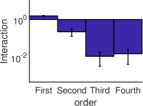
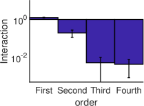
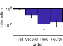
Next, we investigate the HH neuronal network dynamics to confirm that the first two-order effective interactions in the full-order MEP distribution dominate higher-order effective interactions. We evolve HH networks in a long-time simulation of $1.2\times 10^{5}\,\mathrm{s}$ and measure the probability distribution of network states. We have verified that the HH network dynamics in such a long simulation time reaches the steady state, therefore, the measured probability distribution of network states can well represent the true probability distribution of network states. We then calculate effective interactions in the full-order MEP distribution by Eq. (10) from the measured probability distribution of network states. In Fig. 3, the average strength of the $k$th-order effective interactions is computed as the mean of the absolute value of the $k$th-order effective interactions. It can clearly be seen that for three different dynamical regimes, the average strength of effective interactions of high-orders ($\geq 3$) are at least one order of magnitude smaller (in the absolute value) than that of the first-order and the second-order effective interactions.

(a)

(b)

(c)

Figure 3: Hierarchy of effective interactions in the MEP analysis in three dynamical regimes. Mean absolute values of effective interactions from the first-order to the fourth-order for three different dynamical regimes (shown in Fig. 1) are plotted, with the standard deviation indicated by the error bar. Data for these three cases are collected from the three experiments (the same $10$ selected neurons in each case) in Fig. 1, respectively, with a long recording time of $1.2\times 10^{5}\,\mathrm{s}$.

Low-order MEP analysis with short-time recordings

Using the mappings described in the previous sections, we show that the low-order MEP analysis can provide an accurate estimate of the probability distribution of network states with a short-time recording.

First, note that in a short recording of an asynchronous network, the probability of observing a highly-active state (one in which many nodes are active simultaneously) is usually too small to be measured accurately. Thus, the probability distribution of network states measured from the short-time recording cannot capture many network activity states as observed in the long-time recordings (e.g., shown in Fig. 2). Note that the mapping between the probability distribution and effective interactions, i.e., the lower-triangular matrix ${\bf L}_{{\rm JP}}^{(n)}$, suggests that the probability of a highly-active state consists of the summation of many effective interactions. For example, in a small network of $n=2$ nodes, the probability of the highly-active state, $P(\sigma_{1}=1,\sigma_{2}=1)$, can be obtained from Eq. (9) by: $\log P_{11}=J_{0}+J_{1}+J_{2}+J_{12}$. Therefore, to obtain an accurate estimation of such highly-active states, it is important to obtain an accurate estimation of the summation of the effective interactions.

For asynchronous networks, since high-order effective interactions are small (e.g., shown in Fig. 3), the summation in the probability of a highly-active state will be dominated by low-order effective interactions. Note that low-order effective interactions can be derived from low-order moments through an iterative scaling algorithm (see Appendix A for details) in the MEP analysis, and thus an accurate estimation of low-order moments is essential. The mapping between the probability distribution of network states and corresponding moments of the network, i.e., the upper triangular matrix ${\bf U}_{{\rm PM}}^{(n)}$ (Eq. (5)), shows that low-order moments consist of the summation of probabilities of many network activity states. For example, in a network of $n$ nodes, the first-order moment of node 1 is the summation of network state probabilities where node 1 is active (number of $2^{n-1}$ states in total from low-active states to highly-active states), that is $\left\langle\sigma_{1}\right\rangle=P_{10\cdots 0}+P_{11\cdots 0}+\cdots+P_{11\cdots 1}$. Note that low-active states occurs frequently in an asynchronous network; therefore, the summation in low-order moments is dominated by probabilities of these low-active states which can be accurately measured from a short-time recording, leading to good estimation of low-order moments. In addition, we point out that the estimation error in low-order moments can be further reduced due to linear summations. Therefore, one can accurately estimate the low-order moments and perform the low-order MEP analysis in a short-time data recording of network dynamics. It is expected that the low-order MEP distribution provides a good estimate of the probability distribution of network states.

In summary, the low-order MEP distribution can be obtained by the following procedure: First, calculate low-order moments from the experimental short-time recording using Eqs. (1) and (2) for the first-order and the second-order moments, respectively. Second, the low-order MEP analysis (with constraints of low-order moments) is carried out using the iterative scaling algorithm (see Appendix A for details) to derive the low-order effective interactions with all higher-order effective interactions set to zero. This determines $\mathbf{J}^{(n)}$ in Eq. (10), except for $J_{0}$. Third, express the probability distribution, $\mathbf{P}^{(n)}$, as a function of $J_{0}$ using Eq. (10). Finally, determine $J_{0}$ by constraining the summation of all probabilities to equal one. Once all the low-order effective interactions are determined, Eq (4) is used to determine the low-order MEP distribution, e.g., $P_{1}(\Omega)$ and $P_{2}(\Omega)$ represents for the first-order and the second-order MEP distribution, respectively.

Verification for the MEP analysis with short-time recordings by HH neuronal network model

In this section, we use data from the HH neuronal network model to verify that low-order MEP analysis can accurately estimate the probability distribution of network states from short-time recordings using the procedure described in the previous section.

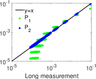
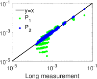
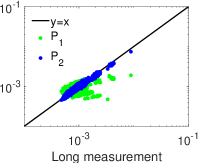
We first evolve the HH neuronal network model with a short simulation time of $120\,\mathrm{s}$ and record the spike trains of the network. Then we estimate the first-order and the second-order moments from this short recording and use these two-order moments to estimate both the first-order and the second-order MEP distributions (Eq. (4)). Finally, we compare the MEP distributions to the probability distribution of network states measured from the long recording of $1.2\times 10^{5}\,\mathrm{s}$. As shown in Fig. 4, for all three dynamical regimes, the probability distribution of the first-order MEP analysis, $P_{1}$ (green), deviates substantially from the measured probability distribution of network states in the long recording. The probability distribution of the second-order MEP analysis, $P_{2}$ (blue), however, is in excellent agreement with the measured probability distribution of network states in the long recording. These results indicate that the low-order, i.e., second-order, MEP analysis provides an efficient method to obtain the probability distribution of network states with short recordings.

(a)

(b)

(c)

Figure 4: First-order and second-order MEP distribution in comparison with the probability distribution of network states. The frequency of each firing state from the distribution of the MEP analysis, $P_{2}$ (blue) and $P_{1}$ (green), is plotted against the frequency measured from the long recording ($1.2\times 10^{5}\,\mathrm{s}$). Data for three different dynamical regimes (shown in Fig. 1) are collected from the three experiments (the same $10$ selected neurons in each case) in Fig. 1, respectively. Here, the MEP analysis is performed with a short recording ($1.2\times 10^{2}\,\mathrm{s}$).

Verification for the MEP analysis with short-time recordings by electrophysiological experiments

In general, it is difficult to obtain a stationary long-time recording of spike trains from the brain of an awake animal in vivo. To verify the validity of the MEP analysis on short recordings, we use the electrophysiological experimental data recorded by multi-electrode array from V1 in anesthetized macaque monkeys in multiple trials. For each trial, an image stimulus was shown on the screen for $100\,\mathrm{ms}$, followed by a $200\,\mathrm{ms}$ uniform gray screen coen2015flexible ; Kohn2015Multi . The number of different images is 956 in total and images are presented in pseudo-random order with each presented $20$ times. Experimental details can be found in Appendix E. Here, we focus on the issue of whether the second-order MEP analysis from a short recording can accurately estimate the probability distribution of neuronal firing patterns in a long recording. Note that the presenting duration for each image is only $2\,\mathrm{s}$, which is too short for the recorded spike trains to have a stable probability distribution. As an alternative, we put the spike trains recorded during the uniform gray screen ($200\,\mathrm{ms}$ in each trial) altogether to obtain a long recording of $3824\,\mathrm{s}$. We have verified that the spike trains in such a long recording has a stable probability distribution. For a short recording, we randomly select $5\%$ length of the long recording, i.e., $191.2\,\mathrm{s}$, and also verified that the probability distribution in such a short recording is quite different from that in the long recording. To perform the MEP analysis, we randomly selected eight neurons’ spike train data from experimental measurements.

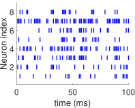
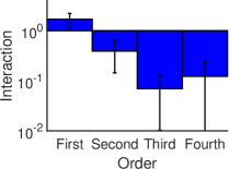
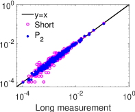
As shown in Fig. 5a, these eight neurons are in an asynchronous state. We then calculate effective interactions in the full-order MEP distribution by Eq. (10) using the measured probability distribution of network states from the long recording of $3824\,\mathrm{s}$. In Fig. 5b, the average strength of the $k$th-order effective interactions is computed as the mean of the absolute value of the $k$th-order effective interactions. It can be seen clearly that the average strength of effective interactions of high-orders ($\geq 3$) are almost one order of magnitude smaller (in the absolute value) than that of the first-order and the second-order effective interactions. Next, we consider a short recording of $191.2\,\mathrm{s}$ and estimate the first-order and the second-order moments from this short recording and use these moments to estimate the second-order MEP distributions (Eq. (4)). As shown in Fig.5c, the probability distribution estimated by the second-order MEP analysis is in excellent agreement with the measured probability distribution of network states in the long recording. However, the probability distribution measured in the short recording clearly deviates from the probability distribution measured in the long recording.

(a)

(b)

(c)

Figure 5: Electrophysiological verification for the second-order MEP analysis with short-time recordings. Spike trains of randomly selected eight neurons are recorded from V1 in anesthetized macaque monkeys (see Appendix E). (a) A short bar indicates that the neuron with certain index fires at certain time. (b) Mean absolute values of effective interactions from the first-order to the fourth-order are plotted, with the standard deviation indicated by the error bar, computed by the long recording of $3824\,\mathrm{s}$. (c) The frequency of each firing state from the distribution measured in the short recording of $191.2\,\mathrm{s}$ (magenta) and the distribution of the second order MEP analysis, $P_{2}$ (blue), is plotted against the frequency measured from the long recording of $3824\,\mathrm{s}$.

Discussion

The second-order MEP analysis has been used to infer the probability distribution of network states under various conditions, such as under spontaneous activity of neuronal networks shlens2006structure ; tang2008maximum or visual input schneidman2006weak . Since the second-order MEP distribution can be obtained by maximizing the Shannon entropy with measured constraints of only the first-order and the second-order moments, the curse of dimensionality is circumvented and an accurate estimation of the probability distribution of network states is provided. A series of works have been initiated to address various aspects of this approach, including explorations of fast algorithms nasser2013spatio ; broderick2007faster , the inference of spatial-temporal correlations tang2008maximum ; shlens2008synchronized ; marre2009prediction ; yeh2010maximum ; nasser2014parameter , and the characterization of network functional connectivity yu2008small ; roudi2009ising ; hertz2011ising ; watanabe2013pairwise ; barton2013ising ; dunn2015correlations .

In addition to spiking neuronal networks schneidman2006weak , the MEP analysis has been applied to analyzing various types of binary data. These applications include, for example, functional magnetic resonance imaging data watanabe2013pairwise , in which each brain region is considered to be either active or silent, and stock market data bury2012statistical , in which the price of each stock is considered to be either increasing or not. However, for all these binary data, long-time recordings are often impractical to be obtained.

In this work, we begin by showing that there exist invertible linear transforms among the probability distribution of network states, the moments, and the effective interactions in the MEP analysis for a general network of nodes with binary dynamics. Based on these transforms, we show that the second-order MEP analysis gives rise to an accurate estimate of the probability distribution of network states with a short-time recording. Finally, using data from both simulated HH neuronal network model and the electrophysiological experiment, we demonstrate the good performance of the second-order MEP analysis with short recordings. Therefore, the applicability of the second-order MEP analysis in practical situations could be significantly improved.

Finally, we point out that there are also some limitations on low-order MEP analysis. First, low-order MEP analysis is often insufficient to accurately reconstruct the probability distribution of network states in synchronized networks since the high-order effective interactions in such cases are often not small xu2016dynamical . Second, as both the order of moment constraints and the network size, $n$, increase, the existing algorithms to estimate effective interactions for a large network become very slow shlens2009structure ; nasser2013spatio . Because the number all network states, i.e., $2^{n}$, is too large when $n$ is a large number, the existing algorithms estimate moments of the MEP distribution using Monte Carlo sampling or its variants from the MEP distribution, which are often very slow when the dimension of the distribution is high shlens2009structure ; nasser2013spatio . Therefore, how to efficiently characterize the statistical properties of strongly-correlated, e.g., nearly synchronized, network dynamics and how to develop fast numerical algorithms for the application of the MEP analysis in large-scale networks remain interesting and challenging issues for future studies.

Appendix A The iterative scaling algorithm

We briefly describe the widely-used numerical algorithm for the estimation of effective interactions from moments. More details about this algorithm can be found in Ref. tang2008maximum . For illustration, we present the procedure to obtain the second-order MEP distribution, $P_{2}(\Omega)$. The interactions are initialized by: $J_{i}=\left\langle\sigma_{i}\right\rangle_{P(\Omega)}$ and $J_{ij}=\left\langle\sigma_{i}\sigma_{j}\right\rangle_{P(\Omega)}$, where $\left\langle\cdot\right\rangle_{P(\Omega)}$ denotes the expectation with respect to the measured probability distribution of network states in data recording, $P(\Omega)$. The expected values of the individual means $\left\langle\sigma_{i}\right\rangle_{P_{2}(\Omega)}$ and pairwise correlations $\left\langle\sigma_{i}\sigma_{j}\right\rangle_{P_{2}(\Omega)}$ with respect to the second-order MEP distribution $P_{2}(\Omega)$ can be determined by

$$\left\langle\sigma_{i}\right\rangle_{P_{2}(\Omega)}\equiv\sum_{l=1}^{2^{n}}\sigma_{i}(\Omega_{l})P_{2}(\Omega_{l}),$$

$$\left\langle\sigma_{i}\sigma_{j}\right\rangle_{P_{2}(\Omega)}\equiv\sum_{l=1}^{2^{n}}\sigma_{i}(\Omega_{l})\sigma_{j}(\Omega_{l})P_{2}(\Omega_{l}),$$

where $\sigma_{i}(\Omega_{l})$ is the state of the $i$th node in the network state $\Omega_{l}$. To improve the agreement between $\left\langle\sigma_{i}\right\rangle_{P_{2}(\Omega)}$, $\left\langle\sigma_{i}\sigma_{j}\right\rangle_{P_{2}(\Omega)}$ and $\left\langle\sigma_{i}\right\rangle_{P(\Omega)}$, $\left\langle\sigma_{i}\sigma_{j}\right\rangle_{P(\Omega)}$, the values of $J_{i}$ and $J_{ij}$ are adjusted by an iterative procedure:

$$J_{i}^{new}=J_{i}^{old}+\alpha\mbox{sign}\left(\left\langle\sigma_{i}\right\rangle_{P(\Omega)}\right)\log\frac{\left\langle\sigma_{i}\right\rangle_{P(\Omega)}}{\left\langle\sigma_{i}\right\rangle_{P_{2}(\Omega)}},$$

$$J_{ij}^{new}=J_{ij}^{old}+\alpha\mbox{sign}\left(\left\langle\sigma_{i}\sigma_{j}\right\rangle_{P(\Omega)}\right)\log\frac{\left\langle\sigma_{i}\sigma_{j}\right\rangle_{P(\Omega)}}{\left\langle\sigma_{i}\sigma_{j}\right\rangle_{P_{2}(\Omega)}},$$

where the constant $\alpha$ is used to maintain the stability of the iteration. We use $\alpha=0.75$ as in Ref. tang2008maximum .

Appendix B The Hodgkin-Huxley neuron model

The HH model is described as follows. The dynamics of the membrane potential of the $i$th neuron, $V_{i}$, is governed by sun2009library ; sun2010pseudo

$$C\frac{\mathrm{d}V_{i}}{\mathrm{d}t} =I_{{\rm Na}}+I_{{\rm K}}+I_{{\rm L}}+I_{i}^{\textrm{input}},$$

$$I_{{\rm Na}} =-(V_{i}-V_{\textrm{Na}})G_{\textrm{Na}}{\rm h}_{i}{\rm m}_{i}^{3},$$

$$I_{{\rm K}} =-(V_{i}-V_{\textrm{K}})G_{\textrm{K}}{\rm n}_{i}^{4},$$

$$I_{{\rm L}} =-(V_{i}-V_{\textrm{L}})G_{\textrm{L}},$$

with

$$\frac{\mathrm{d}X_{i}}{\mathrm{d}t}=(1-X_{i})\alpha_{X}(V_{i})-X_{i}\beta_{X}(V_{i}),$$ (14)

where the gating variable $X={\rm m},{\rm n},{\rm h}$ and

${\displaystyle\alpha_{n}(V_{i})=\frac{0.1-0.01V_{i}}{\exp(1-0.1V_{i})-1}}$,	${\displaystyle\beta_{n}(V_{i})=\frac{5}{40}\exp(-V_{i}/80)}$,
${\displaystyle\alpha_{m}(V_{i})=\frac{2.5-0.1V_{i}}{\exp(2.5-0.1V_{i})-1}}$,	${\displaystyle\beta_{m}(V_{i})=4\exp\left(-V_{i}/18\right)}$,
${\displaystyle\alpha_{h}(V_{i})=0.07\exp(-V_{i}/20)}$,	${\displaystyle\beta_{h}(V_{i})=\frac{1}{\exp(3-0.1V_{i})+1}}$.

The current $I_{i}^{\textrm{input}}$ describes inputs to the $i$th neuron coming from the external drive of the network, as well as interactions between neurons in the network, $I_{i}^{\textrm{input}}=I_{i}^{\textrm{E}}+I_{i}^{\textrm{I}}$ with $I_{i}^{\textrm{E}}=-(V_{i}-V_{G}^{\textrm{E}})G_{i}^{\textrm{E}}$ and $I_{i}^{\textrm{I}}=-(V_{i}-V_{G}^{\textrm{I}})G_{i}^{\textrm{I}}$, where $I_{i}^{\textrm{E}}$ and $I_{i}^{\textrm{I}}$ are excitatory and inhibitory input currents, respectively, and $V_{G}^{\textrm{E}}$ and $V_{G}^{\textrm{I}}$ are their corresponding reversal potentials. The dynamics of the conductance, $G_{i}^{Q}$, for $Q=\textrm{E},\textrm{I}$ are described as follows,

$$\frac{\mathrm{d}G_{i}^{Q}}{\mathrm{d}t} =-\frac{G_{i}^{Q}}{\sigma_{G}^{Q}}+H_{i}^{Q},$$

$$\frac{\mathrm{d}H_{i}^{Q}}{\mathrm{d}t} =-\frac{H_{i}^{Q}}{\sigma_{H}^{Q}}+\sum_{k}F_{i}^{Q}\delta(t-T_{i,k}^{F})+\sum_{j\neq i}C_{ij}g(V_{j}^{\textrm{pre}}),$$

with $g(V_{j}^{\textrm{pre}})=1/\left(1+\exp(-(V_{j}^{\textrm{pre}}-85)/2)\right),$ where $F_{i}^{Q}$ is the strength of the external Poisson input of rate $\mu_{i}$ to neuron $i$ with $T_{i,k}^{F}$ being the time of the $k$th input event. We use $F_{i}^{\textrm{E}}=f$, $F_{i}^{\textrm{I}}=0$, $\mu_{i}=\mu$ for all the neurons in our simulation. The parameter $C_{ij}$ describes the coupling strength from the $j$th presynaptic neuron to the $i$th neuron, and $V_{j}^{\textrm{pre}}$ is the membrane potential of the $j$th presynaptic neuron. The adjacency matrix, $\mathbf{W}=(w_{ij})$, describes the neuronal network connectivity structure and $C_{ij}=w_{ij}C^{Q_{i}Q{}_{j}}$, where $Q_{i}$, $Q_{j}$ is chosen as $E$ or $I$, indicating the neuron type of the $i$th neuron and the $j$th neuron ($C^{Q_{i}Q{}_{j}}$ is one of $C^{\textrm{EE}}$, $C^{\textrm{EI}}$, $C^{\textrm{IE}}$, $C^{\textrm{II}}$). The value $w_{ij}=1$ if there is a directed coupling from the $j$th presynaptic neuron to the $i$th postsynaptic neuron and $w_{ij}=0$ otherwise.

In this study, the values of parameters in the above conductance equations are chosen as: $V_{\textrm{Na}}=115\,\mathrm{mV}$, $V_{\textrm{K}}=-12\,\mathrm{mV}$, $V_{\textrm{L}}=10.6\,\mathrm{mV}$ (the resting potential of a neuron is set to $0\,\mathrm{mV}$), $G_{\textrm{Na}}=120\,\mathrm{mS\cdot cm^{-2}}$, $G_{\textrm{K}}=36\,\mathrm{mS\cdot cm^{-2}}$, $G_{\textrm{L}}=0.3\,\mathrm{mS\cdot cm^{-2}}$, the membrane capacity $C=1\,\mathrm{\mu F\cdot cm^{-2}}$, $V_{G}^{\textrm{E}}=65\,\mathrm{mV}$, $V_{G}^{\textrm{I}}=-15\,\mathrm{mV}$, $\sigma_{G}^{E}=0.5\,\mathrm{ms}$, $\sigma_{H}^{E}=3.0\,\mathrm{ms}$, $\sigma_{G}^{I}=0.5\,\mathrm{ms}$, and $\sigma_{H}^{I}=7.0\,\mathrm{ms}$. We keep the Poisson input parameters fixed during each single simulation.

In our numerical simulation, an explicit fourth order Runge-Kutta method is used sun2009library ; sun2010pseudo with time step $\sim 0.03\,\mathrm{ms}$. The spike train data were obtained with a sufficiently high sampling rate, e.g., $2\,\mathrm{kHz}$.

Appendix C Proof of one-to-one mapping between the probability distribution and moments

We prove that there exists a full-rank matrix ${\bf U}_{{\rm PM}}^{(n)}$ that transforms from $\mathbf{P}^{(n)}$ to $\mathbf{M}^{(n)}$, i.e.,

$${\bf U}_{{\rm PM}}^{(n)}\mathbf{P}^{(n)}=\mathbf{M}^{(n)},$$ (15)

for a network of any size $n$. As an illustration with a network of $n=2$ nodes, the expectation of $\sigma_{1}$, $\sigma_{2}$, $\sigma_{1}\sigma_{2}$ can be obtained by

$$\left[\begin{array}[]{cccc}1&1&1&1\\ 0&1&0&1\\ 0&0&1&1\\ 0&0&0&1\end{array}\right]\left[\begin{array}[]{c}P_{00}\\ P_{10}\\ P_{01}\\ P_{11}\end{array}\right]=\left[\begin{array}[]{c}1\\ \left\langle\sigma_{1}\right\rangle\\ \left\langle\sigma_{2}\right\rangle\\ \left\langle\sigma_{1}\sigma_{2}\right\rangle\end{array}\right],$$ (16)

i.e., $\mathbf{U}_{{\rm PM}}^{(2)}\mathbf{P}^{(2)}=\mathbf{M}^{(2)}$. Clearly, from Eq. (16), $\mathbf{U}_{{\rm PM}}^{(2)}$ is of full rank. We now prove the above result for any $n$ by mathematical induction. Suppose $\mathbf{U}_{{\rm PM}}^{(k)}$ is of full rank. Then $\mathbf{P}^{(k+1)}$ and $\mathbf{M}^{(k+1)}$ can be decomposed into two parts with equal length of $2^{k}$ and $\mathbf{U}_{{\rm PM}}^{(k+1)}$ can be decomposed into four sub-matrices with the dimension of each sub-matrix being $2^{k}\times 2^{k}$ as follows:

$$\left[\begin{array}[]{cc}\mathbf{U}_{11}^{(k+1)}&\mathbf{U}_{12}^{(k+1)}\\ \mathbf{U}_{21}^{(k+1)}&\mathbf{U}_{22}^{(k+1)}\end{array}\right]\left[\begin{array}[]{c}\mathbf{P}_{1}^{(k+1)}\\ \mathbf{P}_{2}^{(k+1)}\end{array}\right]=\left[\begin{array}[]{c}\mathbf{M}_{1}^{(k+1)}\\ \mathbf{M}_{2}^{(k+1)}\end{array}\right],$$

where

$$\mathbf{P}_{1}^{(k+1)}=\left[\begin{array}[]{c}P_{000\cdots 000}\\ P_{100\cdots 000}\\ P_{010\cdots 000}\\ P_{110\cdots 000}\\ \vdots\\ P_{111\cdots 110}\end{array}\right],\quad\quad\mathbf{P}_{2}^{(k+1)}=\left[\begin{array}[]{c}P_{000\cdots 001}\\ P_{100\cdots 001}\\ P_{010\cdots 001}\\ P_{110\cdots 001}\\ \vdots\\ P_{111\cdots 111}\end{array}\right].$$

The expression of $\mathbf{M}_{1}^{(k+1)}$ is the same as the expression of $\mathbf{M}^{(k)}$ in Eq. (6), i.e., $\mathbf{M}_{1}^{(k+1)}=\mathbf{M}^{(k)}$, and $\mathbf{M}_{2}^{(k+1)}$ can be expressed as follows,

$$\mathbf{M}_{2}^{(k+1)}=\left[\begin{array}[]{c}\left\langle 1\cdot\sigma_{k+1}\right\rangle\\ \left\langle\sigma_{1}\sigma_{k+1}\right\rangle\\ \left\langle\sigma_{2}\sigma_{k+1}\right\rangle\\ \left\langle\sigma_{1}\sigma_{2}\sigma_{k+1}\right\rangle\\ \vdots\\ \left\langle\sigma_{2}\prod_{j=3}^{k}\sigma_{j}\sigma_{k+1}\right\rangle\\ \left\langle\sigma_{1}\sigma_{2}\prod_{j=3}^{k}\sigma_{j}\sigma_{k+1}\right\rangle\end{array}\right].$$

In the representation of the base-2 number system of $k+1$ digits, the first digit of the representation of $i-1$, indicating the state of node $k+1$, is $0$ for $1\leq i\leq 2^{k}$ and $1$ for $2^{k}+1\leq i\leq 2^{k+1}.$ For any $i$ with $1\leq i\leq 2^{k}$, suppose $p_{i}^{(k)}$ is the probability of state $(\sigma_{1},\sigma_{2},\cdots,\sigma_{k})$, i.e., $P_{\sigma_{1}\sigma_{2}\cdots,\sigma_{k}}$, then, the $i$th entry of $\mathbf{P}_{1}^{(k+1)}$ and $\mathbf{P}_{2}^{(k+1)}$ are $P_{\sigma_{1}\sigma_{2}\cdots,\sigma_{k},0}$ and $P_{\sigma_{1}\sigma_{2}\cdots,\sigma_{k},1}$, respectively. Thus, the states of nodes from the first to the $2^{k}$th are all the same for $\mathbf{P}^{(k)}$, $\mathbf{P}_{1}^{(k+1)}$ and $\mathbf{P}_{2}^{(k+1)}$. Since $\mathbf{M}_{1}^{(k+1)}$ is the same as $\mathbf{M}^{(k)}$, i.e., their expressions only consider nodes from the first to the $2^{k}$th, the contribution from both $\mathbf{P}_{1}^{(k+1)}$ and $\mathbf{P}_{2}^{(k+1)}$ to $\mathbf{M}_{1}^{(k+1)}$ is the same as the contribution from $\mathbf{P}^{(k)}$ to $\mathbf{M}^{(k)}$, i.e., $\mathbf{U}_{11}^{(k+1)}=\mathbf{U}_{{\rm PM}}^{(k)}$ and $\mathbf{U}_{12}^{(k+1)}=\mathbf{U}_{{\rm PM}}^{(k)}$. Since the state of node $k+1$ is $0$ in all entries of $\mathbf{P}_{1}^{(k+1)}$, there is no contribution of $\mathbf{P}_{1}^{(k+1)}$ to $\mathbf{M}_{2}^{(k+1)}$, i.e., $\mathbf{U}_{21}^{(k+1)}=\mathbf{0}$.

Similarly, since the state of node $k+1$ is $1$ in all entries of $\mathbf{P}_{2}^{(k+1)}$, the contribution from $\mathbf{P}_{2}^{(k+1)}$ to $\mathbf{M}_{2}^{(k+1)}$ only depends on the states of nodes from the first to the $2^{k}$th—there is a one-to-one correspondence of each entry between $\mathbf{P}_{2}^{(k+1)}$ and $\mathbf{P}^{(k)}$, and between $\mathbf{M}_{2}^{(k+1)}$ and $\mathbf{M}^{(k)}$ as aforementioned. Thus, $\mathbf{U}_{22}^{(k+1)}=\mathbf{U}_{{\rm PM}}^{(k)}$ and we can obtain a recursive relation, that is,

$$\mathbf{U}_{{\rm PM}}^{(k+1)}=\left[\begin{array}[]{cc}\mathbf{U}_{{\rm PM}}^{(k)}&\mathbf{U}_{{\rm PM}}^{(k)}\\ \mathbf{0}^{(k)}&\mathbf{U}_{{\rm PM}}^{(k)}\end{array}\right],$$ (17)

where $\mathbf{0}^{(k)}$ is the zero matrix with dimension $2^{k}\times 2^{k}$. Thus, $\mathbf{U}_{{\rm PM}}^{(k+1)}$ is also a matrix of full rank. By induction, $\mathbf{U}_{{\rm PM}}^{(n)}$ is of full rank for any $n$.

Appendix D Proof of the recursive relation among effective interactions

For a network of $n$ nodes, we prove the following recursive relation in the full-order MEP analysis using mathematical induction:

$$J_{12\cdots(k+1)}=J_{12\cdots k}^{1}-J_{12\cdots k},$$ (18)

where the term $J_{12\dots k}^{1}$ is obtained from the $k$th order effective interaction $J_{12...k}$ by changing the state of the $(k+1)$st node in it.

From the mapping between effective interactions and the probability distribution (Eq. (10)), it can be seen that the effective interactions is simply a linear combination of logarithm of the probability distribution. To express this explicitly, we first introduce the notation $H_{m}^{l}$ as

$$H_{m}^{l}=\sum_{\Omega\in\Lambda_{m}^{l}}\log P(\Omega),$$ (19)

where $\Lambda_{m}^{l}=\{(\sigma_{1},\sigma_{2},\cdots,\sigma_{n})|\sum_{i=1}^{m}\sigma_{i}=l;\sigma_{j}=0,m<j\leq n\}$, $0\leq l\leq m\leq n$.

We then show that if the $k$th-order ($1\leq k\leq n$) effective interaction, $J_{12\cdots k}$, can be expressed as

$$J_{12\cdots k}=\sum_{i=0}^{k}(-1)^{k-i}H_{k}^{i},$$ (20)

Eq. (18) is also valid as follows. For $1\leq i\leq k$, there are $i$ nodes out of $k+1$ nodes active in the states described by $H_{k+1}^{i}$ of $\Lambda_{k+1}^{{}^{i}}$. For $0<i<k+1$, we can split $H_{k+1}^{i}$ into two terms, one is $H_{k}^{i}$, where the $(k+1)$st node is inactive, the other term is $W_{k}^{i-1}\equiv H_{k+1}^{i}-H_{k}^{i}$, where the $(k+1)$st node is active. We also define $W_{k}^{k}\equiv H_{k+1}^{k+1}$. From Eq. (20), we have

$$J_{12\cdots(k+1)}=\sum_{i=0}^{k+1}(-1)^{k+1-i}H_{k+1}^{i}.$$

By using $H_{k+1}^{i}=W_{k}^{i-1}+H_{k}^{i}$ and $H_{k+1}^{0}=H_{k}^{0}$, we have

$$J_{12\cdots(k+1)} =H_{k+1}^{k+1}+\sum_{i=1}^{k}(-1)^{k+1-i}(W_{k}^{i-1}+H_{k}^{i})-(-1)^{k}H_{k+1}^{0}$$

$$=W_{k}^{k}+\sum_{i=1}^{k}(-1)^{k+1-i}W_{k}^{i-1}-(-1)^{k}H_{k+1}^{0}-\sum_{i=1}^{k}(-1)^{k-i}H_{k}^{i}$$

$$=\sum_{i=0}^{k}(-1)^{k-i}W_{k}^{i}-\sum_{i=0}^{k}(-1)^{k-i}H_{k}^{i}$$

$$=J_{12\cdots k}^{1}-J_{12\cdots k},$$

where $J_{12\cdots k}^{1}$ is the quantity which switches the state of the $(k+1)$st node in the $k$th-order effective interaction $J_{12...k}$ from inactive to active. Therefore, the recursive relation (Eq. (18)) is proved if Eq. (20) is valid for $1\leq k\leq n$.

We next prove the validity of Eq. (20) by mathematical induction as follows. For $k=1$, as shown in Eq. (11) in the main text, we have

$$J_{1} =\log\frac{P_{10\cdots 0}}{P_{00\cdots 0}}$$

$$=H_{1}^{1}-H_{1}^{0}.$$

Therefore, Eq. (20) is valid when $k=1$. Now, we assume Eq. (20) is valid for $k\leq K$.

We next want to prove that Eq. (20) holds for $k=K+1$. We begin by show that an arbitrary $g$th-order ($g\leq K$) effective interaction $J_{i_{1}\cdots i_{g}}$ can be expressed as follows:

$$J_{i_{1}\cdots i_{g}}=\sum_{i=0}^{g}(-1)^{g-i}H_{A_{g}}^{i},\quad g\leq K$$ (21)

where $A_{g}=\{i_{1},\cdots,i_{g}\}$,

$$H_{A_{g}}^{l}=\sum_{\Omega\in\Lambda_{A_{g}}^{l}}\log P(\Omega),$$

and $\Lambda_{A_{g}}^{l}=\{(\sigma_{i_{1}},\sigma_{i_{2}},\cdots,\sigma_{i_{n}})|\sum_{i_{j}\in A_{g}}\sigma_{i_{j}}=l;\sigma_{i_{j}}=0,g<j\leq n\}$. To show the validity of Eq. (21), we can permute the neuronal indexes from $\{1,2,\cdots,n\}$ to $\{i_{1},i_{2},\cdots,i_{n}\}$ by the mapping $j\rightarrow i_{j}$ for $1\leq j\leq n$. Since Eq. (20) is valid for $g\leq K$ by assumption, Eq. (21) is also valid.

Next, we study the relation between $J_{12\cdots(K+1)}$ and the effective interactions whose orders are smaller than $K+1$. By substituting $\Omega=(1,1,\cdots,1,0,\cdots,0)$ (nodes from $1$ to $K+1$ are active and nodes from $K+2$ to $n$ are inactive) into the full-order MEP analysis, we obtain

$$J_{12\cdots(K+1)}+\sum_{g=1}^{K}\sum_{i_{1}<\cdots<i_{g}}^{K+1}J_{i_{1}\cdots i_{g}}=H_{K+1}^{K+1}-H_{K+1}^{0}.$$ (22)

For $g\leq K$, from Eq (21), by the induction assumption, we have

$$\sum_{i_{1}<\cdots<i_{g}}^{K+1}J_{i_{1}\cdots i_{g}}=\sum_{i=0}^{g}(-1)^{g-i}C_{K+1-i}^{g-i}H_{K+1}^{i},$$ (23)

where $C_{K+1-i}^{g-i}$ is the number of the selection of $g-i$ terms from all the possible $K+1-i$ choices. Since $J_{i_{1}\cdots i_{g}}$ is the $g$th-order effective interaction, as in Eq. (21), the sign of the logarithm probability of a state in which there are $i$ nodes active is $(-1)^{g-i}$. To consider the coefficient of $H_{K+1}^{i}$ in the right hand side of Eq. (23), we can consider that for each group of $i$ nodes, how many groups of $g$ nodes in the left hand side of Eq. (23) containing these considered $i$ nodes, where $g\geq i$. If there are $g$ nodes containing the considered $i$ nodes, then, there are only $g-i$ nodes unknown. These $g-i$ nodes can be chosen from the group of nodes which belongs to the total $K+1$ nodes but not the considered $i$ nodes. Therefore, the choice number of these $g-i$ nodes is $C_{K+1-i}^{g-i}$. Then, we have

$$J_{12\cdots(K+1)}=H_{K+1}^{K+1}-H_{K+1}^{0}-\sum_{g=1}^{K}\sum_{i=0}^{g}(-1)^{g-i}C_{K+1-i}^{g-i}H_{K+1}^{i}.$$ (24)

For $K+1>l>0$, the coefficient of $H_{K+1}^{l}$ is

$$-\sum_{g=l}^{K}(-1)^{g-l}C_{K+1-l}^{g-l}=(-1)^{K+1-l}.$$ (25)

The coefficient of $H_{K+1}^{0}$ is

$$-1-\sum_{g=1}^{K}(-1)^{g}C_{K+1}^{g}=(-1)^{K+1}.$$ (26)

Through Eqs. (24), (26) and (25), we obtain

$$J_{12\cdots(K+1)}=\sum_{i=0}^{K+1}(-1)^{K+1-i}H_{K+1}^{i}.$$ (27)

That is, Eq. (20) is valid for $k=K+1$. By induction, we obtain that Eq. (20) holds for any integer $k$ with $1\leq k\leq n$. Therefore, we prove the validity of Eq. (18).

Appendix E Electrophysiological experiments

The data were collected in the Laboratory of Adam Kohn at the Albert Einstein College of Medicine and downloaded from crcns.org (pvc-8) Kohn2015Multi . These data consist of multi-electrode recordings from V1 in anesthetized macaque monkeys, while natural images and gratings were flashed on the screen. Recordings were performed using the “Utah” electrode array and spike-sorting algorithm was used to determine spike trains corresponding to each single neuron. Natural images were presented at two sizes, $3-6.7$ degrees and windowed to $1$ degree, to quantify surround modulation. All stimuli ($956$ in total) were displayed in pseudo-random order for $100\,\mathrm{ms}$ each, followed by a $200\,\mathrm{ms}$ uniform gray screen. Each stimulus was presented 20 times. Experimental procedures and stimuli are fully described in Ref. coen2015flexible .

References

- (1) J. Barton and S. Cocco, Ising models for neural activity inferred via selective cluster expansion: structural and coding properties, Journal of Statistical Mechanics: Theory and Experiment, 2013 (2013), p. P03002.
- (2) T. Broderick, M. Dudik, G. Tkacik, R. E. Schapire, and W. Bialek, Faster solutions of the inverse pairwise ising problem, arXiv preprint arXiv:0712.2437, (2007).
- (3) T. Bury, Statistical pairwise interaction model of stock market, The European Physical Journal B, 86 (2013), p. 89.
- (4) A. Cavagna, I. Giardina, F. Ginelli, T. Mora, D. Piovani, R. Tavarone, and A. M. Walczak, Dynamical maximum entropy approach to flocking, Physical Review E, 89 (2014), p. 042707.
- (5) R. Coen-Cagli, A. Kohn, and O. Schwartz, Flexible gating of contextual influences in natural vision, Nature neuroscience, (2015).
- (6) B. Dunn, M. Mørreaunet, and Y. Roudi, Correlations and functional connections in a population of grid cells, PLoS Comput Biol, 11 (2015), p. e1004052.
- (7) A. Golan, G. G. Judge, and D. Miller, Maximum entropy econometrics: Robust estimation with limited data, Wiley New York, 1996.
- (8) A. Hernando, R. Hernando, A. Plastino, and A. Plastino, The workings of the maximum entropy principle in collective human behaviour, Journal of The Royal Society Interface, 10 (2013), p. 20120758.
- (9) J. Hertz, Y. Roudi, and J. Tyrcha, Ising models for inferring network structure from spike data, arXiv preprint arXiv:1106.1752, (2011).
- (10) E. T. Jaynes, Information theory and statistical mechanics, Physical review, 106 (1957), p. 620.
- (11) M. P. Karlsson and L. M. Frank, Awake replay of remote experiences in the hippocampus, Nature neuroscience, 12 (2009), p. 913.
- (12) S. Khatiwala, F. Primeau, and T. Hall, Reconstruction of the history of anthropogenic co2 concentrations in the ocean, Nature, 462 (2009), pp. 346–349.
- (13) D. C. Knill and A. Pouget, The bayesian brain: the role of uncertainty in neural coding and computation, TRENDS in Neurosciences, 27 (2004), pp. 712–719.
- (14) A. Kohn and R. Coen-Cagli, Multi-electrode recordings of anesthetized macaque v1 responses to static natural images and gratings., CRCNS.org http://dx.doi.org/10.6080/K0SB43P8, (2015).
- (15) A. B. Mantsyzov, A. S. Maltsev, J. Ying, Y. Shen, G. Hummer, and A. Bax, A maximum entropy approach to the study of residue-specific backbone angle distributions in -synuclein, an intrinsically disordered protein, Protein Science, 23 (2014), pp. 1275–1290.
- (16) O. Marre, S. El Boustani, Y. Frégnac, and A. Destexhe, Prediction of spatiotemporal patterns of neural activity from pairwise correlations, Physical review letters, 102 (2009), p. 138101.
- (17) A. S. Morcos and C. D. Harvey, History-dependent variability in population dynamics during evidence accumulation in cortex, Nature Neuroscience, (2016).
- (18) H. Nasser and B. Cessac, Parameter estimation for spatio-temporal maximum entropy distributions: Application to neural spike trains, Entropy, 16 (2014), pp. 2244–2277.
- (19) H. Nasser, O. Marre, and B. Cessac, Spatio-temporal spike train analysis for large scale networks using the maximum entropy principle and monte carlo method, Journal of Statistical Mechanics: Theory and Experiment, 2013 (2013), p. P03006.
- (20) I. E. Ohiorhenuan, F. Mechler, K. P. Purpura, A. M. Schmid, Q. Hu, and J. D. Victor, Sparse coding and high-order correlations in fine-scale cortical networks, Nature, 466 (2010), pp. 617–621.
- (21) Y. Roudi, J. Tyrcha, and J. Hertz, Ising model for neural data: model quality and approximate methods for extracting functional connectivity, Physical Review E, 79 (2009), p. 051915.
- (22) D. Sakakibara, A. Sasaki, T. Ikeya, J. Hamatsu, T. Hanashima, M. Mishima, M. Yoshimasu, N. Hayashi, T. Mikawa, M. Wälchli, et al., Protein structure determination in living cells by in-cell nmr spectroscopy, Nature, 458 (2009), pp. 102–105.
- (23) S. Saremi and T. J. Sejnowski, Hierarchical model of natural images and the origin of scale invariance, Proceedings of the National Academy of Sciences, 110 (2013), pp. 3071–3076.
- (24) L. Saulis and V. Statulevicius, Limit theorems for large deviations, vol. 73, Springer Science & Business Media, 2012.
- (25) E. Schneidman, M. J. Berry, R. Segev, and W. Bialek, Weak pairwise correlations imply strongly correlated network states in a neural population, Nature, 440 (2006), pp. 1007–1012.
- (26) J. Shlens, G. D. Field, J. L. Gauthier, M. Greschner, A. Sher, A. M. Litke, and E. Chichilnisky, The structure of large-scale synchronized firing in primate retina, The Journal of Neuroscience, 29 (2009), pp. 5022–5031.
- (27) J. Shlens, G. D. Field, J. L. Gauthier, M. I. Grivich, D. Petrusca, A. Sher, A. M. Litke, and E. Chichilnisky, The structure of multi-neuron firing patterns in primate retina, The Journal of neuroscience, 26 (2006), pp. 8254–8266.
- (28) J. Shlens, F. Rieke, and E. Chichilnisky, Synchronized firing in the retina, Current opinion in neurobiology, 18 (2008), pp. 396–402.
- (29) T. Squartini, I. van Lelyveld, and D. Garlaschelli, Early-warning signals of topological collapse in interbank networks, Scientific reports, 3 (2013).
- (30) G. J. Stephens and W. Bialek, Statistical mechanics of letters in words, Physical Review E, 81 (2010), p. 066119.
- (31) J. I. Sułkowska, F. Morcos, M. Weigt, T. Hwa, and J. N. Onuchic, Genomics-aided structure prediction, Proceedings of the National Academy of Sciences, 109 (2012), pp. 10340–10345.
- (32) Y. Sun, D. Zhou, A. Rangan, and D. Cai, Pseudo-lyapunov exponents and predictability of hodgkin-huxley neuronal network dynamics, Journal of computational neuroscience, 28 (2010), pp. 247–266.
- (33) Y. Sun, D. Zhou, A. V. Rangan, and D. Cai, Library-based numerical reduction of the hodgkin–huxley neuron for network simulation, Journal of computational neuroscience, 27 (2009), p. 369.
- (34) A. Tang, D. Jackson, J. Hobbs, W. Chen, J. L. Smith, H. Patel, A. Prieto, D. Petrusca, M. I. Grivich, A. Sher, et al., A maximum entropy model applied to spatial and temporal correlations from cortical networks in vitro, The Journal of Neuroscience, 28 (2008), pp. 505–518.
- (35) T. Watanabe, S. Hirose, H. Wada, Y. Imai, T. Machida, I. Shirouzu, S. Konishi, Y. Miyashita, and N. Masuda, A pairwise maximum entropy model accurately describes resting-state human brain networks, Nature communications, 4 (2013), p. 1370.
- (36) Z.-Q. J. Xu, G. Bi, D. Zhou, and D. Cai, A dynamical state underlying the second order maximum entropy principle in neuronal networks, Communications in Mathematical Sciences, 15 (2017), pp. 665–692.
- (37) F.-C. Yeh, A. Tang, J. P. Hobbs, P. Hottowy, W. Dabrowski, A. Sher, A. Litke, and J. M. Beggs, Maximum entropy approaches to living neural networks, Entropy, 12 (2010), pp. 89–106.
- (38) S. Yu, D. Huang, W. Singer, and D. Nikolić, A small world of neuronal synchrony, Cerebral cortex, 18 (2008), pp. 2891–2901.
- (39) D. Zhou, Y. Xiao, Y. Zhang, Z. Xu, and D. Cai, Granger causality network reconstruction of conductance-based integrate-and-fire neuronal systems, PloS one, 9 (2014), p. e87636.