SPECTRUM-ADAPTED POLYNOMIAL APPROXIMATION FOR MATRIX FUNCTIONS

Abstract

We propose and investigate two new methods to approximate $f({\bf A}){\bf b}$ for large, sparse, Hermitian matrices ${\bf A}$. The main idea behind both methods is to first estimate the spectral density of ${\bf A}$, and then find polynomials of a fixed order that better approximate the function $f$ on areas of the spectrum with a higher density of eigenvalues. Compared to state-of-the-art methods such as the Lanczos method and truncated Chebyshev expansion, the proposed methods tend to provide more accurate approximations of $f({\bf A}){\bf b}$ at lower polynomial orders, and for matrices ${\bf A}$ with a large number of distinct interior eigenvalues and a small spectral width.

Index Terms—  Matrix function, spectral density estimation, polynomial approximation, orthogonal polynomials, graph spectral filtering, weighted least squares polynomial regression.

1 INTRODUCTION

Efficiently computing $f({\bf A}){\bf b}$, a function of a large, sparse Hermitian matrix times a vector, is an important component in numerous signal processing, machine learning, applied mathematics, and computer science tasks. Application examples include graph-based semi-supervised learning methods [2]-[4]; graph spectral filtering in graph signal processing [5]; convolutional neural networks / deep learning [6, 7]; clustering [8, 9]; approximating the spectral density of a large matrix [10]; estimating the numerical rank of a matrix [11, 12]; approximating spectral sums such as the log-determinant of a matrix [13] or the trace of a matrix inverse for applications in physics, biology, information theory, and other disciplines [14]; solving semidefinite programs [15]; simulating random walks [16, Chapter 8]; and solving ordinary and partial differential equations [17]-[19].

References [20, Chapter 13], [21]-[23] survey different approaches to this well-studied problem of efficiently computing

$$f({\bf A}){\bf b}:={\bf V}f({\boldsymbol{\Lambda}}){\bf V}^{\top}{\bf b},$$ (1)

where the columns of ${\bf V}$ are the eigenvectors of the Hermitian matrix ${\bf A}\in\mathbb{R}^{N\times N}$; ${\boldsymbol{\Lambda}}$ is a diagonal matrix whose diagonal elements are the corresponding eigenvalues of ${\bf A}$, which we denote by $\lambda_{1},\lambda_{2},\ldots,\lambda_{N}$; and $f({\boldsymbol{\Lambda}})$ is a diagonal matrix whose $k$th diagonal entry is given by $f(\lambda_{k})$. For large matrices, it is not practical to explicitly compute the eigenvalues of ${\bf A}$ in order to approximate (1). Rather, the most common techniques, all of which avoid a full eigendecomposition of ${\bf A}$, include (i) truncated orthogonal polynomial expansions, including Chebyshev [24]-[26] and Jacobi; (ii) rational approximations [22, Section 3.4]; (iii) Krylov subspace methods such as the Lanczos method [24], [27]-[30]; and (iv) quadrature/contour integral methods [20, Section 13.3].

Our focus in this work is on polynomial approximation methods. Let $p_{K}(\lambda)=c_{0}+\sum_{k=1}^{K}c_{k}\lambda^{k}$ be a degree $K$ polynomial approximation to the function $f$ on a known interval $[\underline{\lambda},\overline{\lambda}]$ containing all of the eigenvalues of ${\bf A}$. Then the approximation $p_{K}({\bf A}){\bf b}$ can be computed recursively, either through a three-term recurrence for specific types of polynomials (see Section 3 for more details), or through a nested multiplication iteration [31, Section 9.2.4], letting ${\bf x}^{(0)}=c_{K}{\bf b}$, and then iterating

$${\bf x}^{(l)}=c_{K-l}{\bf b}+{\bf A}{\bf x}^{(l-1)},~{}l=1,2,\ldots,K.$$

The computational cost of either of these approaches is dominated by multiplying the sparse matrix ${\bf A}$ by $K$ different vectors. The approximation error is bounded by

$$||f({\bf A})-p_{K}({\bf A})||_{2} =\max_{\ell=1,2,\ldots,N}|f(\lambda_{\ell})-p_{K}(\lambda_{\ell})|$$ (2)

$$\leq\sup_{\lambda\in[\underline{\lambda},\overline{\lambda}]}|f(\lambda)-p_{K}(\lambda)|.$$ (3)

If, for example, $p_{K}$ is a degree $K$ truncated Chebyshev series approximation of an analytic function $f$, the upper bound in (3) converges geometrically to 0 as $K$ increases, at a rate of ${\mathcal{O}}\left({\rho^{-K}}\right)$, where $\rho$ is the radius of an open Bernstein ellipse on which $f$ is analytic and bounded (see, e.g., [32, Theorem 5.16], [33, Theorem 8.2]). In addition to the computational efficiency and convergence guarantees, a third advantage of polynomial approximation methods is that they can be implemented in a distributed setting [34]. A fourth advantage is that the $i$th element of $p_{K}({\bf A}){\bf b}$ only depends on the elements of ${\bf b}$ within $K$ hops of $i$ on the graph associated with ${\bf A}$. This localization property is important in many graph-based data analysis applications (e.g., graph spectral filtering [35], deep learning [6]).

While the classical truncated orthogonal polynomial expansion methods (e.g., Chebyshev, Legendre, Jacobi) aim to approximate the function $f$ throughout the full interval $[\underline{\lambda},\overline{\lambda}]$, it is only the polynomial approximation error at the eigenvalues of ${\bf A}$ that affects the overall error in (2). With knowledge of the complete set of eigenvalues, we could do better, for example, by fitting a degree $K$ polynomial via the discrete least squares problem $\min_{p\in{\cal P}_{K}}\sum_{\ell=1}^{N}\left[f(\lambda_{\ell})-p(\lambda_{\ell})\right]^{2}$. In Fig. 1, we show an example of such a discrete least squares fitting. The resulting approximation error $||f({\bf A})-p_{K}({\bf A})||_{2}$ for $K=5$ is 0.020, as opposed to 0.347 for the degree 5 truncated Chebyshev approximation. This is despite the fact that $\sup_{\lambda\in[\underline{\lambda},\overline{\lambda}]}|f(\lambda)-p_{K}(\lambda)|$ is equal to 0.650 for the discrete least squares approximation, as opposed to 0.347 for the Chebyshev approximation.

Fig. 1: Degree 5 polynomial approximations of the function $f(\lambda)=e^{-\lambda}$ of the graph Laplacian of a random Erdös-Renyi graph with 500 vertices and edge probability 0.2. The discrete least squares approximation incurs larger errors in the lower end of the spectrum. However, since the eigenvalues are concentrated at the upper end of the spectrum, it yields a lower approximation error $||f({\bf A})-p_{5}({\bf A})||_{2}$.

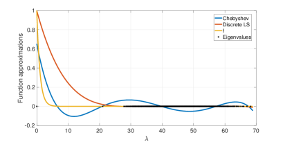
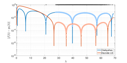
While in our setting we do not have access to the complete set of eigenvalues, our approach in this work is to leverage recent developments in efficiently estimating the spectral density of the matrix ${\bf A}$, to adapt the polynomial to the spectrum in order to achieve better approximation accuracy at the (unknown) eigenvalues. After reviewing spectral density estimation in the next section, we present two new classes of spectrum-adapted approximation techniques in Section 3. We conclude with numerical experiments, and a discussion of the situations in which the proposed methods work better than the state-of-the-art methods.

2 SPECTRAL DENSITY ESTIMATION

The cumulative spectral density function or empirical spectral cumulative distribution of the matrix ${\bf A}$ is defined as

$$P_{\lambda}(z):=\frac{1}{N}\sum_{\ell=1}^{N}1\!\!1_{\left\{\lambda_{\ell}\leq z\right\}},$$ (4)

and the spectral density function [36, Chapter 6]) (also called the Density of States or empirical spectral distribution [37, Chapter 2.4]) of ${\bf A}$ is the probability measure defined as $p_{\lambda}(z):=\frac{1}{N}\sum_{\ell=1}^{N}1\!\!1_{\left\{\lambda_{\ell}=z\right\}}.$ Lin et al. [10] provide an overview of methods to approximate these functions. In this work, we use a variant of the Kernel Polynomial Method (KPM) [38]-[40] described in [10, 41] to estimate the cumulative spectral density function $P_{\lambda}(z)$ of ${\bf A}$. Namely, for each of $T$ linearly spaced points $\xi_{i}$ between $\underline{\lambda}$ and $\overline{\lambda}$, we estimate the number of eigenvalues less than or equal to $\xi_{i}$ via Hutchinson’s stochastic trace estimator [42]:

$$\eta_{i}=\mbox{tr}\bigl{(}\Theta_{\xi_{i}}({\bf A})\bigr{)}=\mathbb{E}[{\bf x}^{\top}\Theta_{\xi_{i}}({\bf A}){\bf x}] \approx\frac{1}{J}\sum_{j=1}^{J}{{\bf x}^{(j)}}^{\top}\tilde{\Theta}_{\xi_{i}}({\bf A}){\bf x}^{(j)},$$ (5)

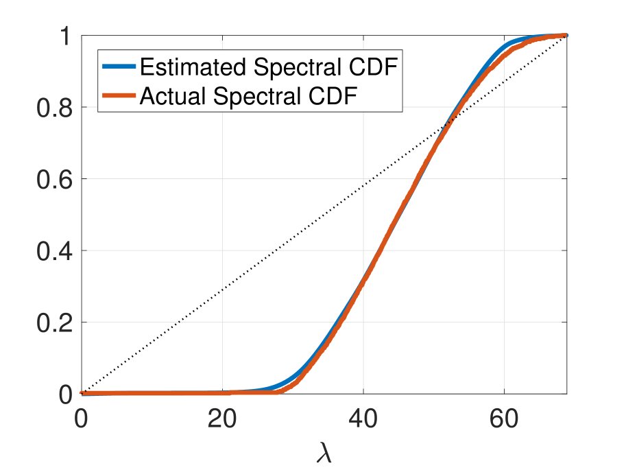
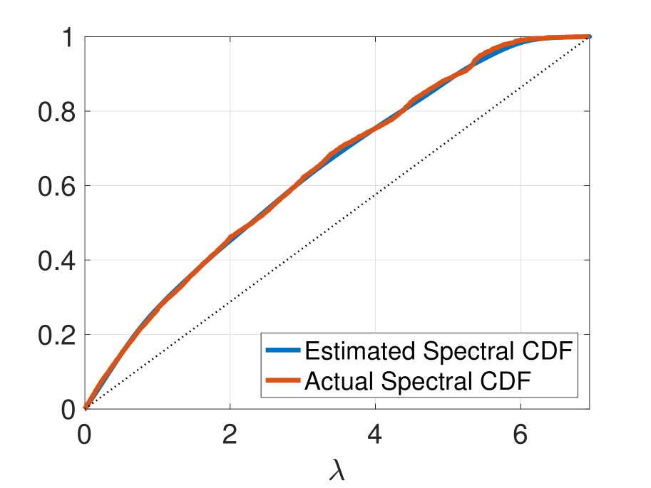
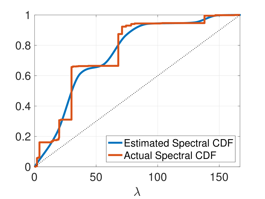
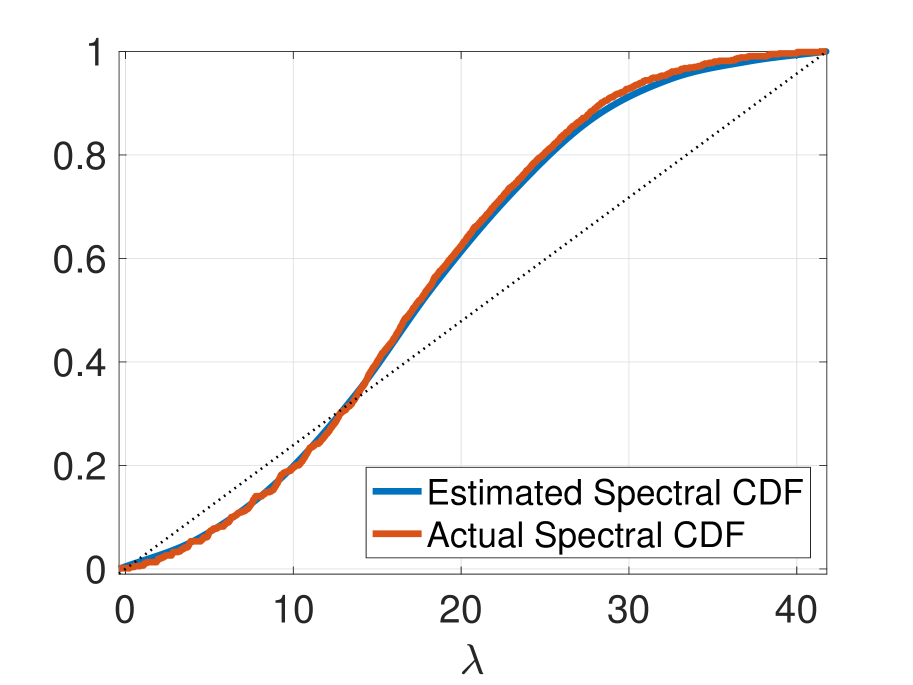
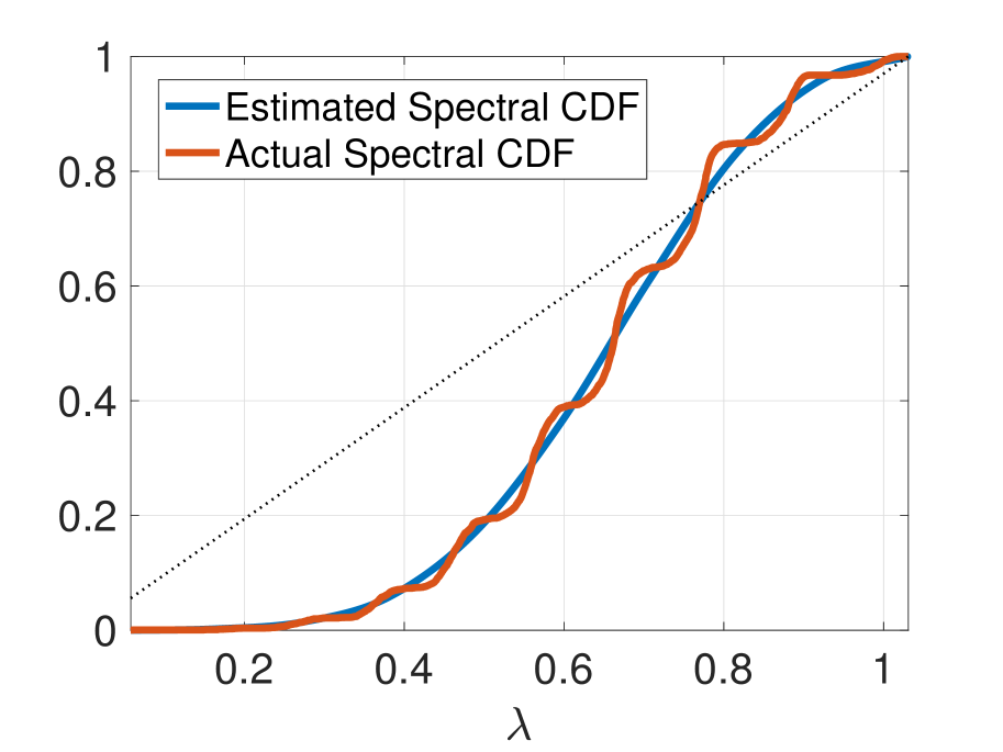
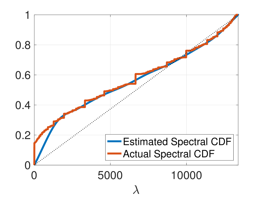
where each ${\bf x}^{(j)}$ is random vector with each component having an independent and identical standard normal distribution, and $\tilde{\Theta}_{\xi_{i}}$ is a Jackson-Chebyshev polynomial approximation to $\Theta_{\xi_{i}}(\lambda):=1\!\!1_{\left\{\lambda\leq\xi_{i}\right\}}$ [43, 44]. As in [45], we then form an approximation $\tilde{P}_{\lambda}(z)$ to $P_{\lambda}(z)$ by performing monotonic piecewise cubic interpolation [46] on the series of points $\left\{\left(\xi_{i},\frac{\eta_{i}}{N}\right)\right\}_{i=1,2,\ldots,T}$. Analytically differentiating $\tilde{P}_{\lambda}(z)$ yields an approximation $\tilde{p}_{\lambda}(z)$ to the spectral density function $p_{\lambda}(z)$. Since $\tilde{P}_{\lambda}(z)$ is a monotonic cubic spline, we can also analytically compute its inverse function $\tilde{P}_{\lambda}^{-1}(y)$. Fig. 2 shows examples of the estimated cumulative spectral density functions for six real, symmetric matrices ${\bf A}$: the graph Laplacians of the Erdös-Renyi graph (gnp) from Fig. 1 and the Minnesota traffic network [47] ($N=2642$), and the net25 ($N=9520$), si2 ($N=769$), cage9 ($N=3534$), and saylr4 ($N=3564$) matrices from the SuiteSparse Matrix Collection [48]. The computational complexity of forming the estimate $\tilde{P}_{\lambda}(z)$ is ${\cal O}(MJK_{\Theta})$, where $M$ is the number of nonzero entries in ${\bf A}$, $J$ is the number of random vectors in (5) (in our experiments, $J=10$ suffices), and $K_{\Theta}$ is the degree of the Jackson-Chebyshev polynomial approximations $\tilde{\Theta}_{\xi_{i}}$ [41]. While this cost is non-negligible if computing $f({\bf A}){\bf b}$ for a single $f$ and a single ${\bf b}$, it only needs to be computed once for each ${\bf A}$ if repeating this calculation for multiple functions $f$ or multiple vectors ${\bf b}$, as is often the case in the applications mentioned above.

    gnp

  

    minnesota

  

    net25

  

    si2

  

    cage9

  

    saylr4

  

Fig. 2: Estimated and actual cumulative spectral density functions for six real, symmetric matrices A. We estimate the eigenvalue counts for $T=10$ linearly spaced points on $[\underline{\lambda},\overline{\lambda}]$ via (5), with degree $K_{\Theta}=30$ polynomials and $J=10$ random vectors ${\bf x}^{(j)}$.

3 SPECTRUM-ADAPTED METHODS

In this section, we introduce two new classes of degree $K$ polynomial approximations $p_{K}({\bf A}){\bf b}$ to $f({\bf A}){\bf b}$, both of which leverage the estimated cumulative spectral density function $\tilde{P}_{\lambda}(z)$.

3.1 Spectrum-adapted polynomial interpolation

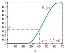
In the first method, we take $y_{k}:=\frac{\cos\left(\frac{k\pi}{K}\right)+1}{2}$, for $k=0,1,\ldots,K$, which are the $K+1$ extrema of the degree $K$ Chebyshev polynomial shifted to the interval $[0,1]$. We then warp these points via the inverse of the estimated cumulative spectral density function by setting $x_{k}=P_{\lambda}^{-1}(y_{k})$, before finding the unique degree $K$ polynomial interpolation through the points $\{(x_{k},f(x_{k}))\}_{k=0,1,\ldots,K}$. As shown in Fig. 3, a higher density of the warped points $\{x_{k}\}$ fall in higher density regions of the spectrum of ${\bf A}$.

Fig. 3: Construction of six interpolation points for the same graph Laplacian matrix described in Fig. 1. The interpolation points $\{x_{k}\}$ on the horizontal axis are computed by applying the inverse of the estimated cumulative spectral density function to the initial Chebyshev points $\{y_{k}\}$ on the vertical axis.

3.2 Spectrum-adapted polynomial regression / orthogonal polynomial expansion

A second approach is to solve the weighted least squares polynomial regression problem

$$\min_{p\in{\cal P}_{K}}\sum_{m=1}^{M}w_{m}\left[f(x_{m})-p(x_{m})\right]^{2},$$

where the abscissae $\{x_{m}\}_{m=1,2,\ldots,M}$ and weights $\{w_{m}\}_{m=1,2,\ldots,M}$ are chosen to capture the estimated spectral density function. We investigated several methods to set the points (e.g., linearly spaced points, Chebyshev points on the interval $[\underline{\lambda},\overline{\lambda}]$, Chebyshev points on each subinterval $[\xi_{i},\xi_{i+1}]$, and warped points via the inverse of the estimated cumulative spectral density function as in Section 3.1) and weights (e.g., the analytically computed estimate $\tilde{p}_{\lambda}$ of the spectral density function, a discrete estimate of the spectral density function based on the eigenvalue counts in (5), the original KPM density of states method based on a truncated Chebyshev expansion [10, Eq. 3.11], or equal weights for warped points). In the numerical experiments, we use $M$ evenly spaced points on the interval $[\underline{\lambda},\overline{\lambda}]$ (i.e., $x_{m}=\frac{m-1}{M-1}(\overline{\lambda}-\underline{\lambda})+\underline{\lambda}$), and set the weights to be $w_{m}=\tilde{p}_{\lambda}(x_{m})$.

An alternative way to view this weighted least squares method [49] is as a truncated expansion in polynomials orthogonal with respect to the discrete measure $d\lambda_{M}$ with finite support at the points $\{x_{m}\}$, and an associated inner product [50, Section 1.1]

$$\langle f,g\rangle_{d\lambda_{M}}=\int_{\mathbb{R}}f(t)g(t)d\lambda_{M}=\sum_{m=1}^{M}w_{m}f(x_{m})g(x_{m}).$$

The $M$ discrete monic orthogonal polynomials $\{\pi_{k,M}\}_{k=0,1,M-1}$ satisfy the three-term recurrence relation [50, Section 1.3]

$$\pi_{k+1,M}(x)=(x-\alpha_{k,M})\pi_{k,M}(x)-\beta_{k,M}\pi_{k-1,M}(x),$$

$$\hskip 115.63243ptk=0,1,\ldots,M-1,$$ (6)

with $\pi_{-1,M}(x)=0$, $\pi_{0,M}(x)=1$, $\beta_{0,M}=\sum_{m=1}^{M}w_{m}$,

$$\alpha_{k,M}=\frac{\langle t\pi_{k,M},\pi_{k,M}\rangle_{d\lambda_{M}}}{\langle\pi_{k,M},\pi_{k,M}\rangle_{d\lambda_{M}}},~{}k=0,1,\ldots,M-1,$$

$$\hbox{and }\beta_{k,M}=\frac{\langle\pi_{k,M},\pi_{k,M}\rangle_{d\lambda_{M}}}{\langle\pi_{k-1,M},\pi_{k-1,M}\rangle_{d\lambda_{M}}},~{}k=1,2,\ldots,M-1.$$

Given the abscissae $\{x_{m}\}$ and weights $\{w_{m}\}$, the three-term recursion coefficients $\{\alpha_{k,M}\}_{k=0,1,\ldots,M-1}$ and $\{\beta_{k,M}\}_{k=1,2,\ldots,M-1}$ can also be computed through a stable Lanczos type algorithm on an $(M+1)\times(M+1)$ matrix [50, Section 2.2.3], [51]. In matrix-vector notation, the vectors ${\boldsymbol{\pi}}_{k,M}\in\mathbb{R}^{M}$, which are the discrete orthogonal polynomials evaluated at the $M$ abscissae, can be computed iteratively by the relation

$${\boldsymbol{\pi}}_{k+1,M}=(\hbox{diag}(\{x_{m}\})-\alpha_{k,M}{\bf I}_{M}){\boldsymbol{\pi}}_{k,M}-\beta_{k,M}{\boldsymbol{\pi}}_{k-1,M},$$

$$\hskip 144.54ptk=0,1,\ldots,M-1,$$

with ${\boldsymbol{\pi}}_{-1,M}={\bf 0}_{M}$ and ${\boldsymbol{\pi}}_{0,M}={\bf 1}_{M}$. Finally, the degree $K$ polynomial approximation to $f({\bf A}){\bf b}$ is computed as

$$p_{K}({\bf A}){\bf b}=\sum_{k=0}^{K}\frac{\langle f,\pi_{k,M}\rangle_{d\lambda_{M}}}{\langle\pi_{k,M},\pi_{k,M}\rangle_{d\lambda_{M}}}\pi_{k,M}({\bf A}){\bf b},$$

with $\pi_{-1,M}({\bf A}){\bf b}={\bf 0}_{N}$, $\pi_{0,M}({\bf A}){\bf b}={\bf b}$, and

$$\pi_{k+1,M}({\bf A}){\bf b}=({\bf A}-\alpha_{k,M}{\bf I}_{N})\pi_{k,M}({\bf A}){\bf b}-\beta_{k,M}\pi_{k-1,M}({\bf A}){\bf b},$$

$$\hskip 79.49744ptk=0,1,\ldots,K-1~{}~{}~{}(\hbox{where }K\leq M-1).$$

We briefly comment on the relationship between the spectrum-adapted approximation proposed in this section and the Lanczos approximation to $f({\bf A}){\bf b}$, which is given by [24], [20, Section 13.2]

$${\bf Q}_{K}f({\bf T}_{K}){\bf Q}_{K}^{\top}{\bf b}=||{\bf b}||_{2}{\bf Q}_{K}f({\bf T}_{K}){\bf e}_{1},$$ (7)

where ${\bf Q}_{K}$ is an $N\times(K+1)$ matrix whose columns form an orthonormal basis for ${\cal K}_{K}({\bf A},{\bf b})=\hbox{span}\left\{{\bf b},{\bf Ab},\ldots,{\bf A}^{K}{\bf b}\right\},$ a Krylov subspace. In (7), ${\bf T}_{K}={\bf Q}_{K}^{\top}{\bf A}{\bf Q}_{K}$ is a $(K+1)\times(K+1)$ tridiagonal Jacobi matrix. The first column of ${\bf Q}_{K}$ is equal to $\frac{{\bf b}}{||{\bf b}||}$. The approximation (7) can also be written as $q_{K}({\bf A}){\bf b}$, where $q_{K}$ is the degree $K$ polynomial that interpolates the function $f$ at the $K+1$ eigenvalues of ${\bf T}_{K}$ [20, Theorem 13.5], [52]. Thus, unlike classical polynomial approximation methods, the Lanczos method is indirectly adapted to the spectrum of ${\bf A}$. The Lanczos method differs from proposed method in that ${\bf T}_{K}$ and the Lanczos approximating polynomial $q_{K}$ depend on the initial vector ${\bf b}$. Specifically, the polynomials $\{\tilde{\pi}_{k}\}$ generated from the three-term recurrence

$$\gamma_{k+1}\tilde{\pi}_{k+1}(x)=(x-\alpha_{k})\tilde{\pi}_{k}(x)-\gamma_{k}\tilde{\pi}_{k-1}(x),$$

with the $\{\alpha_{k}\}_{k=0,1,\ldots,K}$ and $\{\gamma_{k}\}_{k=1,2,\ldots,K}$ coefficients taken from the diagonal and superdiagonal entries of ${\bf T}_{K}$, respectively, are orthogonal with respect to the piecewise-constant measure

$$\mu(x)=\begin{cases}0,&x<\lambda_{1}\\ \sum_{j=1}^{i}[\hat{\bf b}(j)]^{2},&\lambda_{i}\leq x<\lambda_{i+1}\\ \sum_{j=1}^{N}[\hat{\bf b}(j)]^{2}=1,&\lambda_{N}\leq x\end{cases},$$

where $\hat{\bf b}={\bf V}^{\top}{\bf q}_{1}={\bf V}^{\top}\left(\frac{{\bf b}}{||{\bf b}||}\right)$, and $\hat{\bf b}(j)$ is its $jth$ component [53, Theorem 4.2]. If $\hat{\bf b}$ happens to be a constant vector, then $\mu(x)=P_{\lambda}(x)$ from (4). If ${\bf A}$ is a graph Laplacian, $\hat{\bf b}$ is the graph Fourier transform [5] of ${\bf b}$, normalized to have unit energy.

4 NUMERICAL EXAMPLES AND DISCUSSION

    $|f(\lambda)-p_{10}(\lambda)|$

  $\frac{||f({\bf A}){\bf b}-p_{K}({\bf A}){\bf b}||_{2}^{2}}{||f({\bf A}){\bf b}||_{2}^{2}}$

gnp

  

  

minnesota

  

  

net25

  

  

si2

  

  

cage9

  

  

saylr4

  

  

saylr4

(scaled)

  

  

Fig. 4: Approximations of $f({\bf A}){\bf b}$ with $f(\lambda)=e^{-\lambda}$.

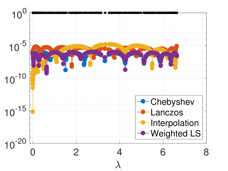
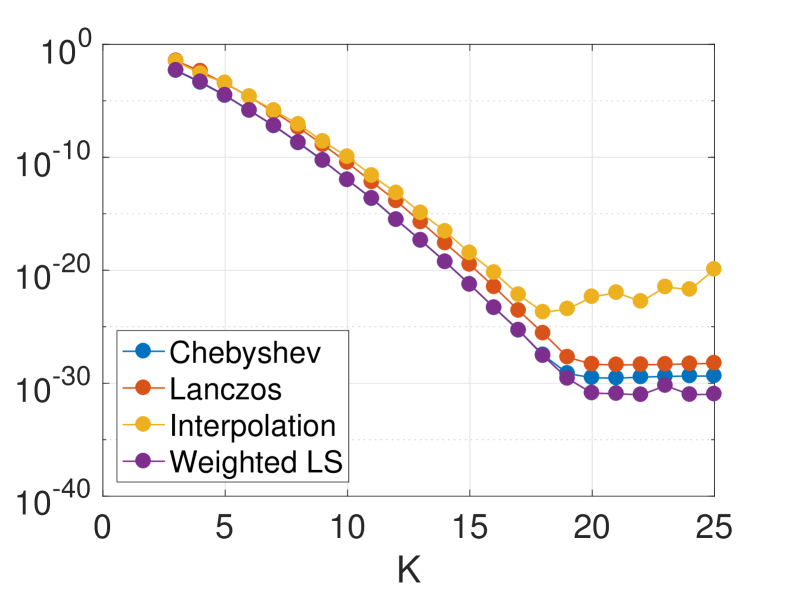
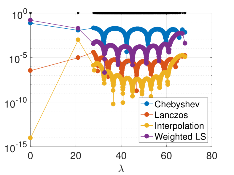
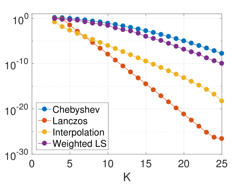
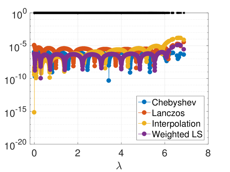
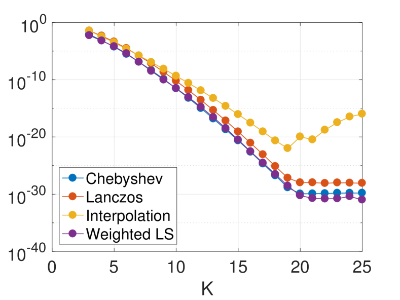
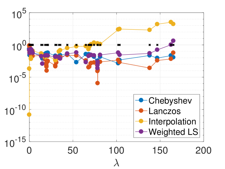
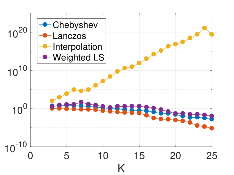
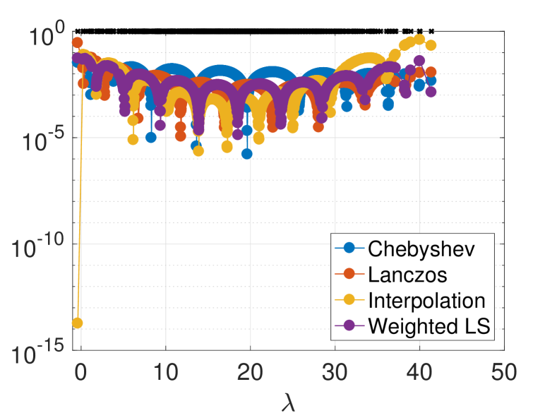
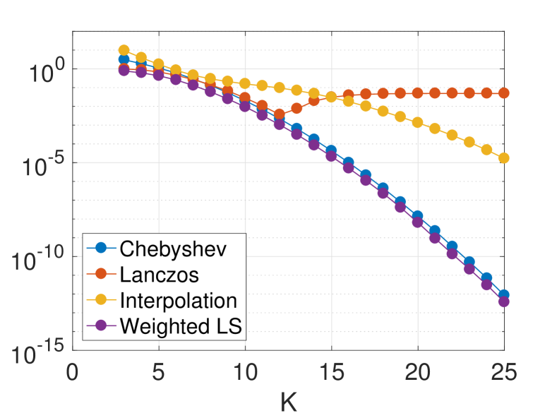
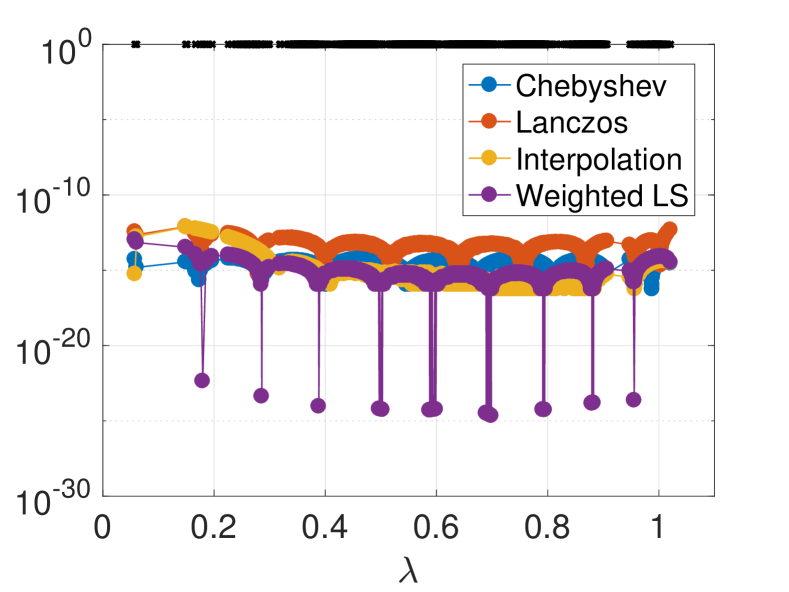
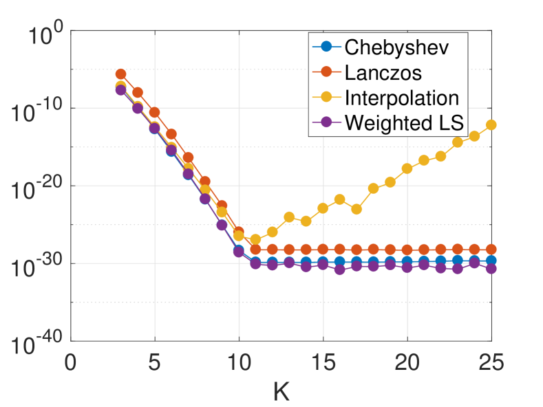
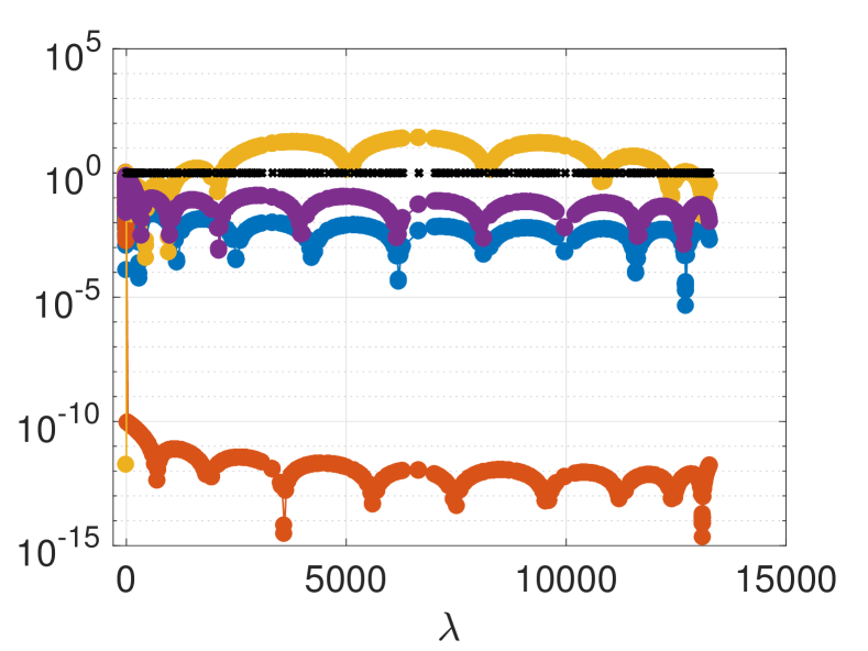
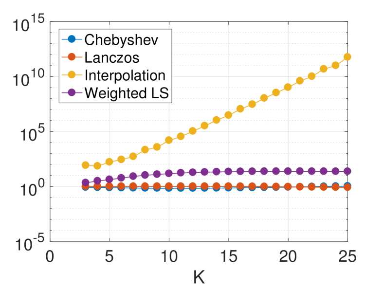
We consider the matrix function $f(\lambda)=e^{-\lambda}$, and approximate $f(\bf A){\bf b}$ with ${\bf b}={\bf V1}$ for different matrices ${\bf A}$ and polynomial approximation orders ranging from $K=3$ to 25. First, we use KPM to estimate the cumulative spectral density function $\tilde{P}_{\lambda}(z)$ with parameters $T=10$, $J=10$, and $K_{\Theta}=30$, as shown in Fig. 2. Based on the analytical derivative and inverse function of $\tilde{P}_{\lambda}(z)$, we obtain the two proposed spectrum-adapted polynomial approximations for $f(\lambda)$, before computing each $p_{K}(\bf A){\bf b}$ via the corresponding three-term recursion. We compare the proposed methods to the truncated Chebyshev expansion and the Lanczos method with the same polynomial order. The results are summarized in Fig. 4. The first column of Fig. 4 displays the errors at all eigenvalues of $\bf A$ for each order 10 polynomial approximation of $f(\lambda)$. The second column examines the convergence of relative errors in approximating $f({\bf A}){\bf b}$ for matrices with various spectral distributions, for each of the four methods. Note that when ${\bf b}$ is a constant vector in the spectral domain of ${\bf A}$, the relative error $\frac{||f({\bf A}){\bf b}-p_{K}({\bf A}){\bf b}||_{2}^{2}}{||f({\bf A}){\bf b}||_{2}^{2}}$ is equal to $\frac{\sum_{\ell=1}^{N}\left(f(\lambda_{\ell})-p_{K}(\lambda_{\ell})\right)^{2}}{\sum_{\ell=1}^{N}f(\lambda_{\ell})^{2}}$, the numerator of which is the discrete least squares objective mentioned in Section 1.

We make a few observations based on the numerical examples:

1. The spectrum-adapted interpolation method often works well for low degree approximations ($K\leq 10$), but is not very stable at higher orders due to ill-conditioning.

2. The Lanczos method is more stable than other methods with respect to the width of the spectrum. To demonstrate this, we scaled the saylr4 matrix by multiplying it by the constant $\frac{1}{2000}$ in the bottom row of Fig. 4. Doing so drastically improves the relative performance of the other methods, even though the spectral distribution is the same.

3. The proposed spectrum-adapted weighted least squares method tends to outperform the Lanczos method for matrices such as si2 and cage9 that have a large number of distinct interior eigenvalues.

4. The proposed spectrum-adapted methods, like the Chebyshev approximation, are amenable to efficient distributed computation via communication between neighboring nodes [34]. The inner products of the Lanczos method may lead to additional communication expense or severe loss of efficiency in certain distributed computation environments (e.g., GPUs).

5 ONGOING WORK

Our ongoing work includes (i) testing the proposed methods on further applications, such as the estimation of the log-determinant of a large sparse Hermitian matrix; (ii) investigating the theoretical manner and rate at which $p_{K}({\bf A}){\bf b}$ converges to $f({\bf A}){\bf b}$ for our new approximation methods; (iii) exploring methods to adapt the approximation to the specific matrix function $f$, in addition to the estimated spectral density of ${\bf A}$; (iv) exploring whether these types of approximations can be used to efficiently compute interior eigenvalues in situations where the Lanczos method struggles; and (v) testing whether it is worthwhile to incorporate our proposed methods into the estimation of the eigenvalue counts in (5), in an iterative fashion, since each $\tilde{\Theta}_{\xi_{i}}({\bf A}){\bf x}^{(j)}$ is itself of the form $f({\bf A}){\bf b}$.

6 References

References

- [1] N. Perraudin, J. Paratte, D. I Shuman, V. Kalofolias, P. Vandergheynst, and D. K. Hammond, “GSPBOX: A toolbox for signal processing on graphs,” arXiv ePrints, 2014, https://lts2.epfl.ch/gsp/.
- [2] A. J. Smola and R. Kondor, “Kernels and regularization on graphs,” in Proc. Ann. Conf. Comp. Learn. Theory, B. Schölkopf and M. Warmuth, Eds., Lect. Notes Comp. Sci., pp. 144–158. Springer, 2003.
- [3] M. Belkin, I. Matveeva, and P. Niyogi, “Regularization and semi-supervised learning on large graphs,” in Learn. Theory, Lect. Notes Comp. Sci., pp. 624–638. Springer-Verlag, 2004.
- [4] D. Zhou, O. Bousquet, T. N. Lal, J. Weston, and B. Schölkopf, “Learning with local and global consistency,” in Adv. Neural Inf. Process. Syst., S. Thrun, L. Saul, and B. Schölkopf, Eds. 2004, vol. 16, pp. 321–328, MIT Press.
- [5] D. I Shuman, S. K. Narang, P. Frossard, A. Ortega, and P. Vandergheynst, “The emerging field of signal processing on graphs: Extending high-dimensional data analysis to networks and other irregular domains,” IEEE Signal Process. Mag., vol. 30, no. 3, pp. 83–98, May 2013.
- [6] M. Defferrard, X. Bresson, and P. Vandergheynst, “Convolutional neural networks on graphs with fast localized spectral filtering,” in Adv. Neural Inf. Process. Syst., 2016, pp. 3844–3852.
- [7] M. M. Bronstein, J. Bruna, Y. LeCun, A. Szlam, and P. Vandergheynst, “Geometric deep learning: Going beyond euclidean data,” IEEE Signal Process. Mag., vol. 34, no. 4, pp. 18–42, 2017.
- [8] N. Tremblay, G. Puy, R. Gribonval, and P. Vandergheynst, “Compressive spectral clustering,” in Proc. Int. Conf. Mach. Learn., 2016, pp. 1002–1011.
- [9] L. Orecchia, S. Sachdeva, and N. K. Vishnoi, “Approximating the exponential, the Lanczos method and an -time spectral algorithm for balanced separator,” in Proc. ACM Symp. Theory Comput., 2012, pp. 1141–1160.
- [10] L. Lin, Y. Saad, and C. Yang, “Approximating spectral densities of large matrices,” SIAM Review, vol. 58, no. 1, pp. 34–65, 2016.
- [11] S. Ubaru and Y. Saad, “Fast methods for estimating the numerical rank of large matrices,” in Proc. Int. Conf. Mach. Learn., New York, NY, Jun. 2016, pp. 468–477.
- [12] S. Ubaru, Y. Saad, and A.-K. Seghouane, “Fast estimation of approximate matrix ranks using spectral densities,” Neural Computation, vol. 29, no. 5, pp. 1317–1351, May 2017.
- [13] S. Ubaru, J. Chen, and Y. Saad, “Fast estimation of tr via stochastic Lanczos quadrature,” SIAM J. Matrix Anal. Appl., vol. 38, no. 4, pp. 1075–1099, 2017.
- [14] I. Han, D. Malioutov, H. Avron, and J. Shin, “Approximating spectral sums of large-scale matrices using stochastic Chebyshev approximations,” SIAM J. Sci. Comput., vol. 39, no. 4, pp. A1558–A1585, 2017.
- [15] S. Arora and S. Kale, “A combinatorial, primal-dual approach to semidefinite programs,” in Proc. ACM Symp. Theory Comput., 2007, pp. 227–236.
- [16] S. Sachdeva and N. K. Vishnoi, “Faster algorithms via approximation theory,” Found. Trends Theor. Comput. Sci., vol. 9, no. 2, pp. 125–210, 2014.
- [17] M. Hochbruck, C. Lubich, and H. Selhofer, “Exponential integrators for large systems of differential equations,” SIAM J. Sci. Comput., vol. 19, no. 5, pp. 1552–1574, 1998.
- [18] R. A. Friesner, L.S. Tuckerman, B.C. Dornblaser, and T. V. Russo, “A method for exponential propagation of large systems of stiff nonlinear differential equations,” J. Sci. Comput., vol. 4, no. 4, pp. 327–354, Dec. 1989.
- [19] E. Gallopoulos and Y. Saad, “Efficient solution of parabolic equations by Krylov approximation methods,” SIAM J. Sci. Stat. Comput., vol. 13, no. 5, pp. 1236–1264, 1992.
- [20] N. J. Higham, Functions of Matrices, SIAM, 2008.
- [21] P. I. Davies and N. J. Higham, “Computing for matrix functions ,” in QCD and Numerical Analysis III, pp. 15–24. Springer, 2005.
- [22] A. Frommer and V. Simoncini, “Matrix functions,” in Model Order Reduction: Theory, Research Aspects and Applications, pp. 275–303. Springer, 2008.
- [23] C. Moler and C. Van Loan, “Nineteen dubious ways to compute the exponential of a matrix, twenty-five years later,” SIAM Rev., vol. 45, no. 1, pp. 3–49, 2003.
- [24] V. L. Druskin and L. A. Knizhnerman, “Two polynomial methods of calculating functions of symmetric matrices,” U.S.S.R. Comput. Maths. Math. Phys., vol. 29, no. 6, pp. 112–121, 1989.
- [25] Y. Saad, “Filtered conjugate residual-type algorithms with applications,” SIAM J. Matrix Anal. Appl., vol. 28, no. 3, pp. 845–870, 2006.
- [26] J. Chen, M. Anitescu, and Y. Saad, “Computing via least squares polynomial approximations,” SIAM J. Sci. Comp., vol. 33, no. 1, pp. 195–222, Feb. 2011.
- [27] V. Druskin and L. Knizhnerman, “Extended Krylov subspaces: Approximation of the matrix square root and related functions,” SIAM J. Matrix Anal. Appl., vol. 19, no. 3, pp. 755–771, 1998.
- [28] M. Eiermann and O. G. Ernst, “A restarted Krylov subspace method for the evaluation of matrix functions,” SIAM J. Numer. Anal., vol. 44, no. 6, pp. 2481–2504, 2006.
- [29] M. Afanasjew, M. Eiermann, O. G. Ernst, and S. Güttel, “Implementation of a restarted Krylov subspace method for the evaluation of matrix functions,” Lin. Alg. Appl., vol. 429, no. 10, pp. 2293–2314, 2008.
- [30] A. Frommer, K. Lund, M. Schweitzer, and D. B. Szyld, “The Radau-Lanczos method for matrix functions,” SIAM J. Matrix Anal. Appl., vol. 38, no. 3, pp. 710–732, 2017.
- [31] G. H. Golub and C. F. Van Loan, Matrix Computations, Johns Hopkins University Press, 2013.
- [32] J. C. Mason and D. C. Handscomb, Chebyshev Polynomials, Chapman and Hall, 2003.
- [33] L. N. Trefethen, Approximation Theory and Approximation Practice, SIAM, 2013.
- [34] D. I Shuman, P. Vandergheynst, D. Kressner, and P. Frossard, “Distributed signal processing via Chebyshev polynomial approximation,” IEEE Trans. Signal Inf. Process. Netw., 2018, in press.
- [35] D. K. Hammond, P. Vandergheynst, and R. Gribonval, “Wavelets on graphs via spectral graph theory,” Appl. Comput. Harmon. Anal., vol. 30, no. 2, pp. 129–150, Mar. 2011.
- [36] P. Van Mieghem, Graph Spectra for Complex Networks, Cambridge University Press, 2011.
- [37] T. Tao, Topics in Random Matrix Theory, American Mathematical Society, 2012.
- [38] R. N. Silver and H. Röder, “Densities of states of mega-dimensional Hamiltonian matrices,” Int. J. Mod. Phys. C, vol. 5, no. 4, pp. 735–753, 1994.
- [39] R. N. Silver, H. Röder, A. F. Voter, and J. D. Kress, “Kernel polynomial approximations for densities of states and spectral functions,” J. Comput. Phys., vol. 124, no. 1, pp. 115–130, 1996.
- [40] L.-W. Wang, “Calculating the density of states and optical-absorption spectra of large quantum systems by the plane-wave moments method,” Phy. Rev. B, vol. 49, no. 15, pp. 10154, 1994.
- [41] S. Li, Y. Jin, and D. I Shuman, “A scalable -channel critically sampled filter bank for graph signals,” arXiv ePrints, 2018.
- [42] M. F. Hutchinson, “A stochastic estimator of the trace of the influence matrix for Laplacian smoothing splines,” Commun. Stat. Simul. Comput., vol. 18, no. 3, pp. 1059–1076, 1989.
- [43] E. Di Napoli, E. Polizzi, and Y. Saad, “Efficient estimation of eigenvalue counts in an interval,” Numer. Linear Algebra Appl., vol. 23, no. 4, pp. 674–692, Aug. 2016.
- [44] G. Puy and P. Pérez, “Structured sampling and fast reconstruction of smooth graph signals,” arXiv e-Prints, 2017.
- [45] D. I Shuman, C. Wiesmeyr, N. Holighaus, and P. Vandergheynst, “Spectrum-adapted tight graph wavelet and vertex-frequency frames,” IEEE Trans. Signal Process., vol. 63, no. 16, pp. 4223–4235, Aug. 2015.
- [46] F. N. Fritsch and R. E. Carlson, “Monotone piecewise cubic interpolation,” SIAM J. Numer. Anal., vol. 17, no. 2, pp. 238–246, Apr. 1980.
- [47] D. Gleich, “The MatlabBGL Matlab library,” http://www.cs.purdue.edu/homes/dgleich/packages/matlab_bgl/index.html.
- [48] T. A. Davis and Y. Hu, “The University of Florida sparse matrix collection,” ACM Trans. Math. Softw., vol. 38, no. 1, pp. 1:1–1:25, 2011.
- [49] G. E. Forsythe, “Generation and use of orthogonal polynomials for data-fitting with a digital computer,” J. SIAM, vol. 5, no. 2, pp. 74–88, 1957.
- [50] W. Gautschi, Orthogonal Polynomials: Computation and Approximation, Oxford University Press, 2004.
- [51] W. B. Gragg and W. J. Harrod, “The numerically stable reconstruction of Jacobi matrices from spectral data,” Numer. Math., vol. 44, no. 3, pp. 317–335, 1984.
- [52] Y. Saad, “Analysis of some Krylov subspace approximations to the matrix exponential operator,” SIAM J. Numer. Anal., vol. 29, no. 1, pp. 209–228, 1992.
- [53] G. H. Golub and G. Meurant, Matrices, Moments and Quadrature with Applications, Princeton University Press, 2010.