The low temperature behavior the Casimir-Polder energy for conductive plane

Nail Khusnutdinov nail.khusnutdinov@gmail.com Centro de Matemática, Computação e Cognição, Universidade Federal do ABC, 09210-170 Santo André, SP, Brazil Institute of Physics, Kazan Federal University, Kremlevskaya 18, Kazan, 420008, Russia    Natalia Emelianova natalia.emelianova@ufabc.edu.br Centro de Matemática, Computação e Cognição, Universidade Federal do ABC, 09210-170 Santo André, SP, Brazil
Abstract

The low temperature expansion of the free energy of atom/plane system is considered for general symmetric form of tensor conductivity of the plane. It is shown that the first correction is proportional to second order of the temperature T2similar-toabsentsuperscript𝑇2\sim T^{2} and comes from TM mode. The agreement of the expansion and exact expressions for different models of conductivity is numerically demonstrated.

pacs:
03.70.+k, 03.50.De

I Introduction

Van der Waals dispersion forces play an important role in different physical, biological as well as chemical phenomena Bordag et al. (2009a); *Parsegian:2006:VdWFHBCEP; *Milonni:1994:QVItQE; *Woods:2016:MpoCavdWi. In the case of interaction between particle and plate it is commonly referred to as the Casimir-Polder force Casimir and Polder (1948). The van der Waals force is very important for interaction of graphene with microparticles Bondarev and Lambin (2005); *Blagov:2007:vdWibmscn; *Churkin:2010:CohaDmodibgaHHoNa; *Khusnutdinov:2011:vdWibaaaasps; *Khusnutdinov:2012:tcpiawsps; *Ribeiro:2013:Svfwg; *Judd:2011:qruaftfgsh, where finite conductivity of graphene plays essential role Khusnutdinov et al. (2016); *Kashapov:2016:TCefpls. At a short range the energy rises as the third power of inverse distance between the microparticle and the plate. The retardation of the interaction should be taken into account at large distances and the interaction energy falls down as the fourth power of distance. At separations larger than a few micrometers, thermal effects become dominant.

Thermal corrections for van der Waalse energy of the system atom/slab and atom/graphene were considered in Ref. Bezerra et al. (2008); *Chaichian:2012:TCiodawg; *Bordag:2014:lteLf; *Khusnutdinov:2018:tccpinp2ddm. It was shown that the correction to the Casimir-Polder free energy is proportional to forth degree of temperature T4similar-toabsentsuperscript𝑇4\sim T^{4} in the case atom and ideal plane. Different models were considered to describe graphene namely, i) hydrodynamical model Barton (2004); *Barton:2005:CefpsIE, ii) density-density correlation function Klimchitskaya et al. (2014) and iii) the Dirac model Castro Neto et al. (2009). In framework of Dirac model was found tensor of conductivity of graphene with and temporal and spatial dispersions and dependence of temperature and chemical potential Bordag et al. (2009b); *Fialkovsky:2011:FCefg; *Bordag:2016:ECefdg; *Bordag:2017:EECefdg.

In the present paper we consider low temperature expansion of the free Casimir-Polder energy for atom/plane system taking into account general symmetric form of the plane’s conductivity tensor. We found that the first correction is quadratic over temperature T2similar-toabsentsuperscript𝑇2\sim T^{2}. Numerically we justify low temperature expansion for three different models of conductivity – constant conductivity model, the Drude-Lorentz model and conductivity calculated in the context of polarization tensor approach.

The paper is organized as follows. In Sec. II, we briefly consider general structure of the conductivity tensor. Section III presents different representations of the Casimir-Polder energy. In Sec. IV we derive the main expressions for low temperature expansion and in Sec. V we numerically compare exact expressions and low temperature approximations. In Sec. VI we discuss the obtained results. Appendix A devotes for different models of graphene’s conductivity and in Appendix B we obtain low temperature expansion of the conductivity.

II The structure of the tensor conductivity

Let us consider conductive 2D2𝐷2D infinitely thin layer positioned perpendicular to axes z𝑧z. We suppose that the anisotropic Ohm low, 𝐣s=𝝈𝐄subscript𝐣𝑠𝝈𝐄\mathbf{j}_{s}=\bm{\sigma}\mathbf{E}, is satisfied on the plane, where 𝐣ssubscript𝐣𝑠\mathbf{j}_{s} is surface current and 𝝈𝝈\bm{\sigma} is conductivity tensor. The latter, in general, depends on the frequency ω𝜔\omega, wave vector 𝒌𝒌\bm{k}, velocity 𝒗𝒗\bm{v} and other scalar parameters such as temperature T𝑇T and chemical potential μ𝜇\mu. It has the following structure Zeitlin (1995) (i,j=x,yformulae-sequence𝑖𝑗𝑥𝑦i,j=x,y)

σij=Aδij+Bkikj+Ck(ivj)+Dvivj+Eεij,\sigma_{ij}=A\delta_{ij}+Bk_{i}k_{j}+Ck_{(i}v_{j)}+Dv_{i}v_{j}+E\varepsilon_{ij}, (1)

where the constant E𝐸E describes parity-odd part of conductivity Fialkovsky and Vassilevich (2009); *Fialkovsky:2012:QFTiG and εijsubscript𝜀𝑖𝑗\varepsilon_{ij} is complete antisymmetric tensor. We consider here parity-even part of conductivity without velocity 𝒗=0𝒗0\bm{v}=0:

σij=Aδij+Bkikj.subscript𝜎𝑖𝑗𝐴subscript𝛿𝑖𝑗𝐵subscript𝑘𝑖subscript𝑘𝑗\sigma_{ij}=A\delta_{ij}+Bk_{i}k_{j}. (2)

The eigenvalues of this tensor,

σte=A,σtm=A+k2B,formulae-sequencesuperscript𝜎te𝐴superscript𝜎tm𝐴superscript𝑘2𝐵\sigma^{\textsf{te}}=A,\ \sigma^{\textsf{tm}}=A+k^{2}B, (3)

are the conductivities of TE and TM modes. Indeed, boundary conditions for TE (Ez=0subscript𝐸𝑧0E_{z}=0) and TM (Hz=0subscript𝐻𝑧0H_{z}=0) modes have the following form

TE ::\displaystyle: [Hz]=0,[Hz]=+4πiωσteHz,formulae-sequencedelimited-[]subscript𝐻𝑧0delimited-[]subscriptsuperscript𝐻𝑧4𝜋i𝜔superscript𝜎tesubscript𝐻𝑧\displaystyle[H_{z}]=0,\ [H^{\prime}_{z}]=+4\pi\mathrm{i}\omega\sigma^{\textsf{te}}H_{z},\allowdisplaybreaks
TM ::\displaystyle: [Ez]=0,[Ez]=4πiωσtmEz,formulae-sequencedelimited-[]subscriptsuperscript𝐸𝑧0delimited-[]subscript𝐸𝑧4𝜋i𝜔superscript𝜎tmsubscriptsuperscript𝐸𝑧\displaystyle[E^{\prime}_{z}]=0,\ [E_{z}]=-\frac{4\pi\mathrm{i}}{\omega}\sigma^{\textsf{tm}}E^{\prime}_{z}, (4)

where [f]=fz0fz+0delimited-[]𝑓subscript𝑓𝑧0subscript𝑓𝑧0[f]=f_{z-0}-f_{z+0} means jump of function at the layer. Therefore, we observe that eigenvalues σtesuperscript𝜎te\sigma^{\textsf{te}} and σtmsuperscript𝜎tm\sigma^{\textsf{tm}} play the role of conductivity for TE and TM modes, respectively.

Using boundary conditions (4) for scattering process we obtain the transmission and reflection coefficients

rte(ω,kz)=ηteηte+kzω,tte=1+rte,formulae-sequencesuperscript𝑟te𝜔subscript𝑘𝑧superscript𝜂tesuperscript𝜂tesubscript𝑘𝑧𝜔superscript𝑡te1superscript𝑟te\displaystyle r^{\textsf{te}}(\omega,k_{z})=-\frac{\eta^{\textsf{te}}}{\eta^{\textsf{te}}+\frac{k_{z}}{\omega}},\ t^{\textsf{te}}=1+r^{\textsf{te}},\allowdisplaybreaks
rtm(ω,kz)=ηtmηtm+ωkz,ttm=1rtm,formulae-sequencesuperscript𝑟tm𝜔subscript𝑘𝑧superscript𝜂tmsuperscript𝜂tm𝜔subscript𝑘𝑧superscript𝑡tm1superscript𝑟tm\displaystyle r^{\textsf{tm}}(\omega,k_{z})=\frac{\eta^{\textsf{tm}}}{\eta^{\textsf{tm}}+\frac{\omega}{k_{z}}},\ t^{\textsf{tm}}=1-r^{\textsf{tm}}, (5)

where kz=ω2k2subscript𝑘𝑧superscript𝜔2superscriptsubscript𝑘perpendicular-to2k_{z}=\sqrt{\omega^{2}-k_{\perp}^{2}} and ηte,tm=2πσte,tmsuperscript𝜂tetm2𝜋superscript𝜎tetm\eta^{\textsf{te},\textsf{tm}}=2\pi\sigma^{\textsf{te},\textsf{tm}}.

III The Casimir-Polder free energy

The system under consideration consists of atom and conductive plane with distance a𝑎a between atom and plane. Using the rarefied procedure of Lifshitz Lifshitz (1956) the Casimir-Polder (CP) energy can be given as a sum of TM and TE contributions Khusnutdinov et al. (2016); *Kashapov:2016:TCefpls,

tmsubscripttm\displaystyle\mathcal{E}_{\textsf{tm}} =\displaystyle= d2k(2π)20dλκα(λ)(λ22κ2)rtm(λ,κ)e2aκ,double-integralsuperscript𝑑2subscript𝑘perpendicular-tosuperscript2𝜋2superscriptsubscript0𝑑𝜆𝜅𝛼𝜆superscript𝜆22superscript𝜅2superscript𝑟tm𝜆𝜅superscript𝑒2𝑎𝜅\displaystyle\iint\frac{d^{2}k_{\perp}}{(2\pi)^{2}}\int_{0}^{\infty}\frac{d\lambda}{\kappa}\alpha(\lambda)\left(\lambda^{2}-2\kappa^{2}\right)r^{\textsf{tm}}(\lambda,\kappa)e^{-2a\kappa},\allowdisplaybreaks
tesubscriptte\displaystyle\mathcal{E}_{\textsf{te}} =\displaystyle= d2k(2π)20dλκα(λ)λ2rte(λ,κ)e2aκ,double-integralsuperscript𝑑2subscript𝑘perpendicular-tosuperscript2𝜋2superscriptsubscript0𝑑𝜆𝜅𝛼𝜆superscript𝜆2superscript𝑟te𝜆𝜅superscript𝑒2𝑎𝜅\displaystyle\iint\frac{d^{2}k_{\perp}}{(2\pi)^{2}}\int_{0}^{\infty}\frac{d\lambda}{\kappa}\alpha(\lambda)\lambda^{2}r^{\textsf{te}}(\lambda,\kappa)e^{-2a\kappa}, (6)

where κ=k2+λ2𝜅superscriptsubscript𝑘perpendicular-to2superscript𝜆2\kappa=\sqrt{k_{\perp}^{2}+\lambda^{2}} and α𝛼\alpha is polarizability of atom.

To take into account temperature we have to change 0dλ2πTn=0\int_{0}^{\infty}d\lambda\to 2\pi T\sum_{n=0}^{\infty}{}^{\prime} and λξn(κκn=k2+ξn2)𝜆subscript𝜉𝑛𝜅subscript𝜅𝑛superscriptsubscript𝑘perpendicular-to2superscriptsubscript𝜉𝑛2\lambda\to\xi_{n}\ (\kappa\to\kappa_{n}=\sqrt{k_{\perp}^{2}+\xi_{n}^{2}}), where ξn=2πnTsubscript𝜉𝑛2𝜋𝑛𝑇\xi_{n}=2\pi nT being the Matsubara frequencies. We obtain the following expressions for free energy Khusnutdinov et al. (2018)

tmsubscripttm\displaystyle\mathcal{F}_{\textsf{tm}} =\displaystyle= T2πn=0d2kκnαn(ξn22κn2)rtm(ξn,κn)e2aκn,𝑇2𝜋superscriptsuperscriptsubscript𝑛0double-integralsuperscript𝑑2subscript𝑘perpendicular-tosubscript𝜅𝑛subscript𝛼𝑛superscriptsubscript𝜉𝑛22superscriptsubscript𝜅𝑛2superscript𝑟tmsubscript𝜉𝑛subscript𝜅𝑛superscript𝑒2𝑎subscript𝜅𝑛\displaystyle\frac{T}{2\pi}\sum_{n=0}^{\infty}{\!}^{\prime}\!\iint\!\frac{d^{2}k_{\perp}}{\kappa_{n}}\alpha_{n}\left(\xi_{n}^{2}-2\kappa_{n}^{2}\right)r^{\textsf{tm}}(\xi_{n},\kappa_{n})e^{-2a\kappa_{n}},\allowdisplaybreaks
tesubscriptte\displaystyle\mathcal{F}_{\textsf{te}} =\displaystyle= T2πn=0d2kκnαnξn2rte(ξn,κn)e2aκn,𝑇2𝜋superscriptsuperscriptsubscript𝑛0double-integralsuperscript𝑑2subscript𝑘perpendicular-tosubscript𝜅𝑛subscript𝛼𝑛superscriptsubscript𝜉𝑛2superscript𝑟tesubscript𝜉𝑛subscript𝜅𝑛superscript𝑒2𝑎subscript𝜅𝑛\displaystyle\frac{T}{2\pi}\sum_{n=0}^{\infty}{\!}^{\prime}\iint\frac{d^{2}k_{\perp}}{\kappa_{n}}\alpha_{n}\xi_{n}^{2}r^{\textsf{te}}(\xi_{n},\kappa_{n})e^{-2a\kappa_{n}}, (7)

where αn=α(ξn)subscript𝛼𝑛𝛼subscript𝜉𝑛\alpha_{n}=\alpha(\xi_{n}). The ideal case appears by formal limit ηnte,tm(rte1,rtm1)subscriptsuperscript𝜂tetm𝑛formulae-sequencesuperscript𝑟te1superscript𝑟tm1\eta^{\textsf{te},\textsf{tm}}_{n}\to\infty\ (r^{\textsf{te}}\to-1,r^{\textsf{tm}}\to 1).

Taking into account the Poisson summation formula (see, for example, Ref. Bordag et al. (2009a)) we obtain following expression for free energy

tmCPsubscripttmsubscriptCP\displaystyle\frac{\mathcal{F}_{\textsf{tm}}}{\mathcal{E}_{\textsf{CP}}} =\displaystyle= 83l=00z3𝑑z01𝑑xcos(zxlaT)83superscriptsubscript𝑙0superscriptsuperscriptsubscript0superscript𝑧3differential-d𝑧superscriptsubscript01differential-d𝑥𝑧𝑥𝑙𝑎𝑇\displaystyle-\frac{8}{3}\sum_{l=0}^{\infty}{}^{\prime}\int_{0}^{\infty}z^{3}dz\int_{0}^{1}dx\cos\left(\frac{zxl}{aT}\right)\allowdisplaybreaks
×\displaystyle\times α(λ)α(0)(x22)rtm(x,1)e2z,𝛼𝜆𝛼0superscript𝑥22superscript𝑟tm𝑥1superscript𝑒2𝑧\displaystyle\frac{\alpha(\lambda)}{\alpha(0)}\left(x^{2}-2\right)r^{\textsf{tm}}(x,1)e^{-2z},\allowdisplaybreaks
teCPsubscripttesubscriptCP\displaystyle\frac{\mathcal{F}_{\textsf{te}}}{\mathcal{E}_{\textsf{CP}}} =\displaystyle= 83l=00z3𝑑z01𝑑xcos(zxlaT)83superscriptsubscript𝑙0superscriptsuperscriptsubscript0superscript𝑧3differential-d𝑧superscriptsubscript01differential-d𝑥𝑧𝑥𝑙𝑎𝑇\displaystyle-\frac{8}{3}\sum_{l=0}^{\infty}{}^{\prime}\int_{0}^{\infty}z^{3}dz\int_{0}^{1}dx\cos\left(\frac{zxl}{aT}\right)\allowdisplaybreaks (8)
×\displaystyle\times α(λ)α(0)x2rte(x,1)e2z,𝛼𝜆𝛼0superscript𝑥2superscript𝑟te𝑥1superscript𝑒2𝑧\displaystyle\frac{\alpha(\lambda)}{\alpha(0)}x^{2}r^{\textsf{te}}(x,1)e^{-2z},

normalized to the CP=3α(0)/8πa4subscriptCP3𝛼08𝜋superscript𝑎4\mathcal{E}_{\textsf{CP}}=-3\alpha(0)/8\pi a^{4} – Casimir-Polder energy for ideal plane/atom. Here λ=zxa,k=za1x2formulae-sequence𝜆𝑧𝑥𝑎𝑘𝑧𝑎1superscript𝑥2\lambda=\frac{zx}{a},\ k=\frac{z}{a}\sqrt{1-x^{2}} and the prime means factor 1/2121/2 for l=0𝑙0l=0. This form is more suitable for analysis at low temperature. Zero terms, l=0𝑙0l=0, in (8) coincides exactly with that obtained for zero temperature in Ref. Khusnutdinov et al. (2016); *Kashapov:2016:TCefpls (see Eq. (6)) but with temperature and chemical potential dependence through the conductivity. We extract the zero term

=tm+te=0+Δsubscripttmsubscripttesubscript0Δ\mathcal{F}=\mathcal{F}_{\textsf{tm}}+\mathcal{F}_{\textsf{te}}=\mathcal{F}_{0}+\Delta\mathcal{F} (9)

and consider low temperature expansion for ΔΔ\Delta\mathcal{F} and 0subscript0\mathcal{F}_{0} separately.

IV The low temperature expansions

To analyze ΔΔ\Delta\mathcal{F} (9) we use Erdélyi’s lemmas for asymptotic expansion integrals Fedoryuk (1977). For completeness we reproduce them below.

Lemma 1

0axβ1f(x)eiΛx𝑑x=n=0anΛ(n+β),superscriptsubscript0𝑎superscript𝑥𝛽1𝑓𝑥superscript𝑒𝑖Λ𝑥differential-d𝑥superscriptsubscript𝑛0subscript𝑎𝑛superscriptΛ𝑛𝛽\int_{0}^{a}x^{\beta-1}f(x)e^{i\Lambda x}dx=\sum_{n=0}^{\infty}a_{n}\Lambda^{-(n+\beta)}, (10)

where

an=f(n)(0)Γ(n+β)n!eiπ2(n+β).subscript𝑎𝑛superscript𝑓𝑛0Γ𝑛𝛽𝑛superscript𝑒𝑖𝜋2𝑛𝛽a_{n}=f^{(n)}(0)\frac{\Gamma\left(n+\beta\right)}{n!}e^{\frac{i\pi}{2}(n+\beta)}.

Lemma 2

0axβ1f(x)lnxeiΛxdx=n=0bn(Λ)Λ(n+β),superscriptsubscript0𝑎superscript𝑥𝛽1𝑓𝑥𝑥superscript𝑒𝑖Λ𝑥𝑑𝑥superscriptsubscript𝑛0subscript𝑏𝑛ΛsuperscriptΛ𝑛𝛽\int_{0}^{a}x^{\beta-1}f(x)\ln xe^{i\Lambda x}dx=\sum_{n=0}^{\infty}b_{n}(\Lambda)\Lambda^{-(n+\beta)}, (11)

where

bn=f(n)(0)Γ(n+β)n!eiπ2(n+β)subscript𝑏𝑛superscript𝑓𝑛0Γ𝑛𝛽𝑛superscript𝑒𝑖𝜋2𝑛𝛽\displaystyle b_{n}=f^{(n)}(0)\frac{\Gamma\left(n+\beta\right)}{n!}e^{\frac{i\pi}{2}(n+\beta)}\allowdisplaybreaks
×[lnΛ+ψ(n+β)+iπ2],absentdelimited-[]Λ𝜓𝑛𝛽𝑖𝜋2\displaystyle\times\left[-\ln\Lambda+\psi\left(n+\beta\right)+\frac{i\pi}{2}\right],

and ψ(x)=Γ(x)/Γ(x)𝜓𝑥superscriptΓ𝑥Γ𝑥\psi(x)=\Gamma^{\prime}(x)/\Gamma(x). Both Lemmas are valid as ΛΛ\Lambda\to\infty, f(n)(a)=0superscript𝑓𝑛𝑎0f^{(n)}(a)=0 and β>0𝛽0\beta>0.

The free Casimir-Polder energy ΔΔ\Delta\mathcal{F} maybe represented in the following form

ΔCP=83l=10𝑑zeiΛz(Ytm+Yte),ΔsubscriptCP83superscriptsubscript𝑙1superscriptsubscript0differential-d𝑧superscript𝑒𝑖Λ𝑧subscript𝑌tmsubscript𝑌te\frac{\Delta\mathcal{F}}{\mathcal{E}_{\textsf{CP}}}=\frac{8}{3}\Re\sum_{l=1}^{\infty}\int_{0}^{\infty}dze^{i\Lambda z}\left(Y_{\textsf{tm}}+Y_{\textsf{te}}\right), (12)

where Λ=laTΛ𝑙𝑎𝑇\Lambda=\frac{l}{aT} and

Ytm(z)subscript𝑌tm𝑧\displaystyle Y_{\textsf{tm}}(z) =\displaystyle= α(λ)α(0)ze2ss(2s2z2)s+z/ηtm𝑑s,𝛼𝜆𝛼0superscriptsubscript𝑧superscript𝑒2𝑠𝑠2superscript𝑠2superscript𝑧2𝑠𝑧subscript𝜂tmdifferential-d𝑠\displaystyle\frac{\alpha(\lambda)}{\alpha(0)}\int_{z}^{\infty}\frac{e^{-2s}s\left(2s^{2}-z^{2}\right)}{s+z/\eta_{\textsf{tm}}}ds,\allowdisplaybreaks
Yte(z)subscript𝑌te𝑧\displaystyle Y_{\textsf{te}}(z) =\displaystyle= α(λ)α(0)ze2sz3z+s/ηte𝑑s.𝛼𝜆𝛼0superscriptsubscript𝑧superscript𝑒2𝑠superscript𝑧3𝑧𝑠subscript𝜂tedifferential-d𝑠\displaystyle\frac{\alpha(\lambda)}{\alpha(0)}\int_{z}^{\infty}\frac{e^{-2s}z^{3}}{z+s/\eta_{\textsf{te}}}ds. (13)

Here λ=z/a𝜆𝑧𝑎\lambda=z/a and k=s2z2/a𝑘superscript𝑠2superscript𝑧2𝑎k=\sqrt{s^{2}-z^{2}}/a are used for frequency and wave-vector, correspondingly.

First of all, let us consider the case without spatial dispersion, η=η(λ)𝜂𝜂𝜆\eta=\eta(\lambda). Straightforward integration in Eq. (13) gives

Ytmsubscript𝑌tm\displaystyle Y_{\textsf{tm}} =\displaystyle= αe2z2α(0)ηtm3{ηtm(2z2z(1+2z)ηtm+(1+z)2ηtm2)\displaystyle\frac{\alpha e^{-2z}}{2\alpha(0)\eta^{3}_{\textsf{tm}}}\left\{\eta_{\textsf{tm}}\left(2z^{2}-z(1+2z)\eta_{\textsf{tm}}+(1+z)^{2}\eta^{2}_{\textsf{tm}}\right)\right.\allowdisplaybreaks
+\displaystyle+ 2z3(ηtm22)e2z(1+ηtm1)Γ(0,2z(1+ηtm1))},\displaystyle\left.2z^{3}(\eta^{2}_{\textsf{tm}}-2)e^{2z\left(1+\eta^{-1}_{\textsf{tm}}\right)}\Gamma\left(0,2z\left(1+\eta^{-1}_{\textsf{tm}}\right)\right)\right\},\allowdisplaybreaks
Ytesubscript𝑌te\displaystyle Y_{\textsf{te}} =\displaystyle= αηteα(0)z3e2zηteΓ(0,2z(1+ηte)),𝛼subscript𝜂te𝛼0superscript𝑧3superscript𝑒2𝑧subscript𝜂teΓ02𝑧1subscript𝜂te\displaystyle\frac{\alpha\eta_{\textsf{te}}}{\alpha(0)}z^{3}e^{2z\eta_{\textsf{te}}}\Gamma\left(0,2z(1+\eta_{\textsf{te}})\right), (14)

where Γ(a,b)Γ𝑎𝑏\Gamma(a,b) is incomplete gamma function.

Expansion at point z=0𝑧0z=0 contents logarithmic contribution

Ytm,te=m=0Amtm,tezm+lnzm=3Bmtm,tezm.subscript𝑌tmtesuperscriptsubscript𝑚0superscriptsubscript𝐴𝑚tmtesuperscript𝑧𝑚𝑧superscriptsubscript𝑚3superscriptsubscript𝐵𝑚tmtesuperscript𝑧𝑚Y_{\textsf{tm},\textsf{te}}=\sum_{m=0}^{\infty}A_{m}^{\textsf{tm},\textsf{te}}z^{m}+\ln z\sum_{m=3}^{\infty}B_{m}^{\textsf{tm},\textsf{te}}z^{m}. (15)

Taking into account this expansion and Lemmas we obtain expansion up to 4th power of T𝑇T for the energy at low temperature

Δtm,teCP=χ29A1tm,te+χ490{A3tm,te\displaystyle\frac{\Delta\mathcal{F}_{\textsf{tm},\textsf{te}}}{\mathcal{E}_{\textsf{CP}}}=-\frac{\chi^{2}}{9}A_{1}^{\textsf{tm},\textsf{te}}+\frac{\chi^{4}}{90}\left\{A_{3}^{\textsf{tm},\textsf{te}}\right.\allowdisplaybreaks
+B3tm,te(lnχ2πγE+90ζR(4)π4+116)},\displaystyle+\left.B_{3}^{\textsf{tm},\textsf{te}}\left(\ln\frac{\chi}{2\pi}-\gamma_{E}+\frac{90\zeta^{\prime}_{R}(4)}{\pi^{4}}+\frac{11}{6}\right)\right\}, (16)

where χ=2πaT𝜒2𝜋𝑎𝑇\chi=2\pi aT and ζR(s)subscript𝜁𝑅𝑠\zeta_{R}(s) is Riemann zeta-function.

From Eqs. (14) we obtain in manifest form

A1tmsuperscriptsubscript𝐴1tm\displaystyle A_{1}^{\textsf{tm}} =\displaystyle= 12ηtm,A1te=0,12subscript𝜂tmsuperscriptsubscript𝐴1te0\displaystyle-\frac{1}{2\eta_{\textsf{tm}}},\ A_{1}^{\textsf{te}}=0,\allowdisplaybreaks
A3tmsuperscriptsubscript𝐴3tm\displaystyle A_{3}^{\textsf{tm}} =\displaystyle= 14a2ηtm(α′′αηtm′′ηtm+2ηtm2ηtm2)2ηtmaηtm314superscript𝑎2subscript𝜂tmsuperscript𝛼′′𝛼subscriptsuperscript𝜂′′tmsubscript𝜂tm2subscriptsuperscript𝜂2tmsubscriptsuperscript𝜂2tm2subscriptsuperscript𝜂tm𝑎subscriptsuperscript𝜂3tm\displaystyle-\frac{1}{4a^{2}\eta_{\textsf{tm}}}\left(\frac{\alpha^{\prime\prime}}{\alpha}-\frac{\eta^{\prime\prime}_{\textsf{tm}}}{\eta_{\textsf{tm}}}+\frac{2\eta^{\prime 2}_{\textsf{tm}}}{\eta^{2}_{\textsf{tm}}}\right)-\frac{2\eta^{\prime}_{\textsf{tm}}}{a\eta^{3}_{\textsf{tm}}}\allowdisplaybreaks
\displaystyle- 2ηtm2+1ηtm+13+(γE+ln[2(1+ηtm)ηtm])B3tm,2subscriptsuperscript𝜂2tm1subscript𝜂tm13subscript𝛾𝐸21subscript𝜂tmsubscript𝜂tmsuperscriptsubscript𝐵3tm\displaystyle\frac{2}{\eta^{2}_{\textsf{tm}}}+\frac{1}{\eta_{\textsf{tm}}}+\frac{1}{3}+\left(\gamma_{E}+\ln\left[\frac{2(1+\eta_{\textsf{tm}})}{\eta_{\textsf{tm}}}\right]\right)B_{3}^{\textsf{tm}},\allowdisplaybreaks
A3tesuperscriptsubscript𝐴3te\displaystyle A_{3}^{\textsf{te}} =\displaystyle= (γE+ln[2(1+ηte)])B3te,subscript𝛾𝐸21subscript𝜂tesubscript𝐵3superscriptte\displaystyle\left(\gamma_{E}+\ln\left[2(1+\eta_{\textsf{te}})\right]\right)B_{3}⁝^{\textsf{te}},\allowdisplaybreaks
B3tmsuperscriptsubscript𝐵3tm\displaystyle B_{3}^{\textsf{tm}} =\displaystyle= 2ηtm31ηtm,B3te=ηte.2subscriptsuperscript𝜂3tm1subscript𝜂tmsuperscriptsubscript𝐵3tesubscript𝜂te\displaystyle\frac{2}{\eta^{3}_{\textsf{tm}}}-\frac{1}{\eta_{\textsf{tm}}},\ B_{3}^{\textsf{te}}=-\eta_{\textsf{te}}. (17)

Taking into account these expressions we obtain asymptotic expansion of free CP energy

ΔtmCPΔsubscripttmsubscriptCP\displaystyle\frac{\Delta\mathcal{F}_{\textsf{tm}}}{\mathcal{E}_{\textsf{CP}}} =\displaystyle= χ218ηtm+χ4270{16ηtm2(1+ηtmaηtm)\displaystyle\frac{\chi^{2}}{18\eta_{\textsf{tm}}}+\frac{\chi^{4}}{270}\left\{1-\frac{6}{\eta^{2}_{\textsf{tm}}}\left(1+\frac{\eta^{\prime}_{\textsf{tm}}}{a\eta_{\textsf{tm}}}\right)\right.\allowdisplaybreaks
\displaystyle- 12ηtm(5+540ζR(4)π4+6ln[χ1+ηtmπηtm]\displaystyle\left.\frac{1}{2\eta_{\textsf{tm}}}\left(5+\frac{540\zeta^{\prime}_{R}(4)}{\pi^{4}}+6\ln\left[\chi\frac{1+\eta_{\textsf{tm}}}{\pi\eta_{\textsf{tm}}}\right]\right.\right.\allowdisplaybreaks
+\displaystyle+ 32a2(α′′αηtm′′ηtm+2ηtm2ηtm2))\displaystyle\left.\left.\frac{3}{2a^{2}}\left(\frac{\alpha^{\prime\prime}}{\alpha}-\frac{\eta^{\prime\prime}_{\textsf{tm}}}{\eta_{\textsf{tm}}}+\frac{2\eta^{\prime 2}_{\textsf{tm}}}{\eta^{2}_{\textsf{tm}}}\right)\right)\right.\allowdisplaybreaks
+\displaystyle+ 6ηtm3(116+ln[χ1+ηtmπηtm]+90ζR(4)π4)},\displaystyle\left.\frac{6}{\eta^{3}_{\textsf{tm}}}\left(\frac{11}{6}+\ln\left[\chi\frac{1+\eta_{\textsf{tm}}}{\pi\eta_{\textsf{tm}}}\right]+\frac{90\zeta^{\prime}_{R}(4)}{\pi^{4}}\right)\right\},\allowdisplaybreaks
ΔteCPΔsubscripttesubscriptCP\displaystyle\frac{\Delta\mathcal{F}_{\textsf{te}}}{\mathcal{E}_{\textsf{CP}}} =\displaystyle= χ4ηte90{116+ln[χ1+ηteπ]+90ζR(4)π4},superscript𝜒4subscript𝜂te90116𝜒1subscript𝜂te𝜋90subscriptsuperscript𝜁𝑅4superscript𝜋4\displaystyle-\frac{\chi^{4}\eta_{\textsf{te}}}{90}\left\{\frac{11}{6}+\ln\left[\chi\frac{1+\eta_{\textsf{te}}}{\pi}\right]+\frac{90\zeta^{\prime}_{R}(4)}{\pi^{4}}\right\}, (18)

where functions α𝛼\alpha and η𝜂\eta and their derivatives are considered at zero argument.

In ideal case Bezerra et al. (2008) the free energy for low temperatures has first correction χ4similar-toabsentsuperscript𝜒4\sim\chi^{4}

CP|T0=1χ4135.evaluated-atsubscriptCP𝑇01superscript𝜒4135\left.\frac{\mathcal{F}}{\mathcal{E}_{\textsf{CP}}}\right|_{T\to 0}=1-\frac{\chi^{4}}{135}. (19)

One comment is in order. Above expansions are valid if arguments of incomplete gamma functions in Eqs. (14) are small, that is for χηtm1+ηtmmuch-less-than𝜒subscript𝜂tm1subscript𝜂tm\chi\ll\frac{\eta_{\textsf{tm}}}{1+\eta_{\textsf{tm}}} and χ11+ηtemuch-less-than𝜒11subscript𝜂te\chi\ll\frac{1}{1+\eta_{\textsf{te}}}. Therefore, we may take limit to ideal case only for TM mode in Eq. (18). To consider ideal case for TE mode we have to take limit ηtesubscript𝜂te\eta_{\textsf{te}}\to\infty first of all in Eq. (14) and then make expansion over z𝑧z.

The main term of expansion χ2/18ηtmsuperscript𝜒218subscript𝜂tm\chi^{2}/18\eta_{\textsf{tm}} is the same for k0𝑘0k\not=0. Indeed, to obtain A1tmsuperscriptsubscript𝐴1tmA_{1}^{\textsf{tm}} we may take derivative of Eq. (13) with respect of z𝑧z and then take limit z0𝑧0z\to 0. By proceed that way we obtain the same form of main term where ηtmsubscript𝜂tm\eta_{\textsf{tm}} is calculated for λ=k=0𝜆𝑘0\lambda=k=0.

Therefore, we observe that for all models of conductivities the main term of low temperature expansion proportional to χ2superscript𝜒2\chi^{2}.

Let us consider now zero term in Poisson representation 0=tm0+tm0subscript0subscriptsuperscript0tmsubscriptsuperscript0tm\mathcal{F}_{0}=\mathcal{F}^{0}_{\textsf{tm}}+\mathcal{F}^{0}_{\textsf{tm}}

tm0CPsubscriptsuperscript0tmsubscriptCP\displaystyle\frac{\mathcal{F}^{0}_{\textsf{tm}}}{\mathcal{E}_{\textsf{CP}}} =\displaystyle= 430z3𝑑z01𝑑xα(λ)α(0)(x22)rtm(x,1)e2z,43superscriptsubscript0superscript𝑧3differential-d𝑧superscriptsubscript01differential-d𝑥𝛼𝜆𝛼0superscript𝑥22superscript𝑟tm𝑥1superscript𝑒2𝑧\displaystyle-\frac{4}{3}\int_{0}^{\infty}z^{3}dz\int_{0}^{1}dx\frac{\alpha(\lambda)}{\alpha(0)}\left(x^{2}-2\right)r^{\textsf{tm}}(x,1)e^{-2z},\allowdisplaybreaks
te0CPsubscriptsuperscript0tesubscriptCP\displaystyle\frac{\mathcal{F}^{0}_{\textsf{te}}}{\mathcal{E}_{\textsf{CP}}} =\displaystyle= 430z3𝑑z01𝑑xα(λ)α(0)x2rte(x,1)e2z.43superscriptsubscript0superscript𝑧3differential-d𝑧superscriptsubscript01differential-d𝑥𝛼𝜆𝛼0superscript𝑥2superscript𝑟te𝑥1superscript𝑒2𝑧\displaystyle-\frac{4}{3}\int_{0}^{\infty}z^{3}dz\int_{0}^{1}dx\frac{\alpha(\lambda)}{\alpha(0)}x^{2}r^{\textsf{te}}(x,1)e^{-2z}. (20)

As noted above it coincides exactly with that obtained for zero temperature in Ref. Khusnutdinov et al. (2016); *Kashapov:2016:TCefpls, but with additional dependence on the temperature and chemical potential through dependence of conductivity on these parameters (see Sec. A.3). These expressions tend to 1/2121/2 for ideal (η𝜂\eta\to\infty) case and for a𝑎a\to\infty.

V Numerical analysis

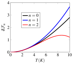
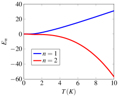
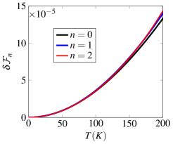
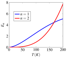
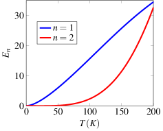
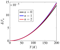
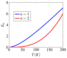
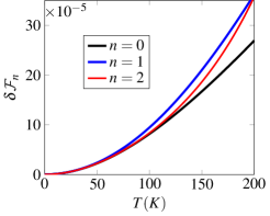
Let us compare numerically the formulas obtained (18) with exact numerical calculations for different models of conductivity. Let us denote for simplicity δn=Δ/CP𝛿subscript𝑛ΔsubscriptCP\delta\mathcal{F}_{n}=\Delta\mathcal{F}/\mathcal{E}_{\textsf{CP}} where n=0𝑛0n=0 corresponds to exact expression calculated numerically and n=1,2𝑛12n=1,2 corresponds to first (χ2similar-toabsentsuperscript𝜒2\sim\chi^{2}) and second (χ4similar-toabsentsuperscript𝜒4\sim\chi^{4}) approximations in (18). Numerically we use (7) and subtract (20). To estimate error we plot relative error function En=(δnδ0)/δ0100%subscript𝐸𝑛𝛿subscript𝑛𝛿subscript0𝛿subscript0percent100E_{n}=(\delta\mathcal{F}_{n}-\delta\mathcal{F}_{0})/\delta\mathcal{F}_{0}\cdot 100\%.

For definiteness we consider Hydrogen atom in framework of one-oscillator model (see Ref. Khusnutdinov et al. (2016)) and distance a=10nm𝑎10𝑛𝑚a=10nm between atom and plane of graphene. Then the interval of temperatures T[0,100]K𝑇0superscript100𝐾T\in[0,100^{\circ}]K corresponds to interval of parameter χ[0,2.7]103𝜒02.7superscript103\chi\in[0,2.7]\cdot 10^{-3}. Different models of graphene’s conductivity briefly discussed in Appendix A.

V.1 Constant conductivity model

First model is constant conductivity model. For graphene we use universal conductivity, σgr=e2/4subscript𝜎𝑔𝑟superscript𝑒24Planck-constant-over-2-pi\sigma_{gr}=e^{2}/4\hbar and then ηtm=ηte=ηgr=0.0114subscript𝜂tmsubscript𝜂tesubscript𝜂𝑔𝑟0.0114\eta_{\textsf{tm}}=\eta_{\textsf{te}}=\eta_{gr}=0.0114. Fig. 1 illustrates numerical evaluation exact expression and approximations obtained and relative error.
Refer to caption
Refer to caption
Figure 1: Constant conductivity model of graphene ηtm=ηte=0.0114subscript𝜂tmsubscript𝜂te0.0114\eta_{\textsf{tm}}=\eta_{\textsf{te}}=0.0114 and Hydrogen atom at distance a=10nm𝑎10𝑛𝑚a=10nm from graphene. Left panel: δn=Δ/CP𝛿subscript𝑛ΔsubscriptCP\delta\mathcal{F}_{n}=\Delta\mathcal{F}/\mathcal{E}_{\textsf{CP}}. n=0𝑛0n=0 is numeric simulation, n=1𝑛1n=1 is approximation up to T2superscript𝑇2T^{2}, n=2𝑛2n=2 is approximation up to T4superscript𝑇4T^{4}. Right panel: relative error in percents.

We observe that relative error for second approximation is not more then 1%percent11\% up to T=100K𝑇100𝐾T=100K.

V.2 Drude-Lorentz model

In the case of Drude-Lorentz 7-oscillator model of conductivity agreement is not so good. The point is that even the conductivity at zero frequency equals to graphene universal conductivity, but derivatives of first and second order are very huge. The contributions to χ4superscript𝜒4\chi^{4} contain terms

η=0.0114,ηaη=8.76103,η′′a2η=1.85107,formulae-sequence𝜂0.0114formulae-sequencesuperscript𝜂𝑎𝜂8.76superscript103superscript𝜂′′superscript𝑎2𝜂1.85superscript107\eta=0.0114,\ \frac{\eta^{\prime}}{a\eta}=8.76\cdot 10^{3},\ \frac{\eta^{\prime\prime}}{a^{2}\eta}=-1.85\cdot 10^{7}, (21)

and the ratio of second term χ4similar-toabsentsuperscript𝜒4\sim\chi^{4} and first χ2similar-toabsentsuperscript𝜒2\sim\chi^{2} is 0.670.670.67 for T=10K𝑇superscript10𝐾T=10^{\circ}K and 676767 for T=100K𝑇superscript100𝐾T=100^{\circ}K.

Refer to caption
Refer to caption
Figure 2: The Drude-Lorentz model of graphene’s conductivity and Hydrogen atom at distance a=10nm𝑎10𝑛𝑚a=10nm from graphene. Left panel: δn=Δ/CP𝛿subscript𝑛ΔsubscriptCP\delta\mathcal{F}_{n}=\Delta\mathcal{F}/\mathcal{E}_{\textsf{CP}}. n=0𝑛0n=0 is numeric simulation, n=1𝑛1n=1 is approximation up to T2superscript𝑇2T^{2}, n=2𝑛2n=2 is approximation up to T4superscript𝑇4T^{4}. Right panel: relative error in percents.

For this reason the low temperature expansion is valid for very low temperature (see Fig. 2).

V.3 Polarization tensor approach

The last model is polarization tensor model of conductivity developed in Refs. Bordag et al. (2009b); *Fialkovsky:2011:FCefg; *Bordag:2016:ECefdg; *Bordag:2017:EECefdg. In this case the conductivity depends on frequency, wave-vector, temperature and chemical potential ηtm,te(λ,k,T,μ)subscript𝜂tmte𝜆𝑘𝑇𝜇\eta_{\textsf{tm},\textsf{te}}(\lambda,k,T,\mu). In the case under consideration, k=0𝑘0k=0,

ηtm,teηgr=4mπλ{1+(λ2m)21(λ2m)arctan(λ2m)}subscript𝜂tmtesubscript𝜂𝑔𝑟4𝑚𝜋𝜆1superscript𝜆2𝑚21𝜆2𝑚𝜆2𝑚\displaystyle\frac{\eta_{\textsf{tm},\textsf{te}}}{\eta_{gr}}=\frac{4m}{\pi\lambda}\left\{1+\frac{\left(\frac{\lambda}{2m}\right)^{2}-1}{\left(\frac{\lambda}{2m}\right)}\arctan\left(\frac{\lambda}{2m}\right)\right\}\allowdisplaybreaks
+16πλm𝑑zz2+m24z2+λ2{1ez+μT+1+1ezμT+1}.16𝜋𝜆superscriptsubscript𝑚differential-d𝑧superscript𝑧2superscript𝑚24superscript𝑧2superscript𝜆21superscript𝑒𝑧𝜇𝑇11superscript𝑒𝑧𝜇𝑇1\displaystyle+\frac{16}{\pi\lambda}\int_{m}^{\infty}dz\frac{z^{2}+m^{2}}{4z^{2}+\lambda^{2}}\left\{\frac{1}{e^{\frac{z+\mu}{T}}+1}+\frac{1}{e^{\frac{z-\mu}{T}}+1}\right\}. (22)
Refer to caption
Refer to caption
Figure 3: Polarization tensor approach for conductivity with m=μ=0𝑚𝜇0m=\mu=0 and γ=0.1eV𝛾0.1𝑒𝑉\gamma=0.1eV at distance a=10nm𝑎10𝑛𝑚a=10nm from graphene. Left panel: δn=Δ/CP𝛿subscript𝑛ΔsubscriptCP\delta\mathcal{F}_{n}=\Delta\mathcal{F}/\mathcal{E}_{\textsf{CP}}. n=0𝑛0n=0 is numeric simulation, n=1𝑛1n=1 is approximation up to T2superscript𝑇2T^{2}, n=2𝑛2n=2 is approximation up to T4superscript𝑇4T^{4}. Right panel: relative error in percents.

In the static limit, λ0𝜆0\lambda\to 0, the conductivity is divergent (but transmission and reflection coefficients (5) tend to that for ideal case). To make it finite we cut λ𝜆\lambda on minimal value γ𝛾\gamma. The threshold parameter γ𝛾\gamma appears in natural way in framework of Kubo approach calculation of conductivity Falkovsky and Varlamov (2007) as a scattering rate.
Refer to caption
Refer to caption
Figure 4: Polarization tensor approach for conductivity with m=0.1eV,μ=0.05eVformulae-sequence𝑚0.1𝑒𝑉𝜇0.05𝑒𝑉m=0.1eV,\mu=0.05eV and γ=0.1eV𝛾0.1𝑒𝑉\gamma=0.1eV at distance a=10nm𝑎10𝑛𝑚a=10nm from graphene. Left panel: δn=Δ/CP𝛿subscript𝑛ΔsubscriptCP\delta\mathcal{F}_{n}=\Delta\mathcal{F}/\mathcal{E}_{\textsf{CP}}. n=0𝑛0n=0 is numeric simulation, n=1𝑛1n=1 is approximation up to T2superscript𝑇2T^{2}, n=2𝑛2n=2 is approximation up to T4superscript𝑇4T^{4}. Right panel: relative error in percents.

Numerical evaluations (see Figs. 3, 4) demonstrate good agreement expansion (18) with exact expression (7).

Let us consider now zero temperature term 0subscript0\mathcal{F}_{0} given by Eqs. (9), (20). In the framework of the model under consideration it depends on the temperature and chemical potential. Expansion of conductivity over temperature is given in Appendix B.

For m=μ=0𝑚𝜇0m=\mu=0 the first correction T3similar-toabsentsuperscript𝑇3\sim T^{3} (see Eq. (54)) and reads

ηte=ηtm=ηgr+48πζR(3)T3λ3.subscript𝜂tesubscript𝜂tmsubscript𝜂𝑔𝑟48𝜋subscript𝜁𝑅3superscript𝑇3superscript𝜆3\eta_{\textsf{te}}=\eta_{\textsf{tm}}=\eta_{gr}+\frac{48}{\pi}\zeta_{R}(3)\frac{T^{3}}{\lambda^{3}}. (23)

Therefore,

0CP=0T=0CP+T3βsubscript0subscriptCPsuperscriptsubscript0𝑇0subscriptCPsuperscript𝑇3𝛽\frac{\mathcal{F}_{0}}{\mathcal{E}_{\textsf{CP}}}=\frac{\mathcal{F}_{0}^{T=0}}{\mathcal{E}_{\textsf{CP}}}+T^{3}\beta (24)

where

β𝛽\displaystyle\beta =\displaystyle= 64ζR(3)ηgrπ0z3𝑑z01𝑑xα(λ)α(0)xe2zλ364subscript𝜁𝑅3subscript𝜂𝑔𝑟𝜋superscriptsubscript0superscript𝑧3differential-d𝑧superscriptsubscript01differential-d𝑥𝛼𝜆𝛼0𝑥superscript𝑒2𝑧superscript𝜆3\displaystyle\frac{64\zeta_{R}(3)\eta_{gr}}{\pi}\int_{0}^{\infty}z^{3}dz\int_{0}^{1}dx\frac{\alpha(\lambda)}{\alpha(0)}\frac{xe^{-2z}}{\lambda^{3}}\allowdisplaybreaks (25)
×\displaystyle\times {2x2(x+ηgr)2+x2(1+xηgr)2}.2superscript𝑥2superscript𝑥subscript𝜂𝑔𝑟2superscript𝑥2superscript1𝑥subscript𝜂𝑔𝑟2\displaystyle\left\{\frac{2-x^{2}}{(x+\eta_{gr})^{2}}+\frac{x^{2}}{(1+x\eta_{gr})^{2}}\right\}.

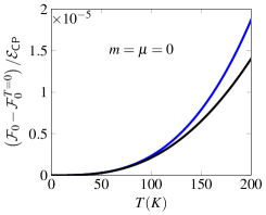
For a=10nm𝑎10𝑛𝑚a=10nm and γ=0.1eV𝛾0.1𝑒𝑉\gamma=0.1eV we have β=2.331012𝛽2.33superscript1012\beta=2.33\cdot 10^{-12} where T(K)𝑇𝐾T(K).

For m=0.1eV𝑚0.1𝑒𝑉m=0.1eV and μ=0.05eV𝜇0.05𝑒𝑉\mu=0.05eV the first correction is exponentially small emμTsimilar-toabsentsuperscript𝑒𝑚𝜇𝑇\sim e^{-\frac{m-\mu}{T}} (see Eq. (50)).

Refer to caption
Refer to caption
Figure 5: Polarization tensor approach for conductivity. Zero term (00T=0)/CPsubscript0superscriptsubscript0𝑇0subscriptCP\left(\mathcal{F}_{0}-\mathcal{F}_{0}^{T=0}\right)/\mathcal{E}_{\textsf{CP}}. Left panel: m=μ=0𝑚𝜇0m=\mu=0 and γ=0.1eV𝛾0.1𝑒𝑉\gamma=0.1eV. Black curve is exact expression (20) and blue is first approximation (24). Right panel: m=0.1eV,μ=0.05eVformulae-sequence𝑚0.1𝑒𝑉𝜇0.05𝑒𝑉m=0.1eV,\mu=0.05eV and γ=0.1eV𝛾0.1𝑒𝑉\gamma=0.1eV. Temperature contribution is exponentially small up 100Ksuperscript100𝐾100^{\circ}K.

Fig. 5 illustrates temperature correction of zero temperature term due to conductivity dependence of temperature and chemical potential.

VI Conclusion

We have obtained the analytic expression of low temperature expansion of the Casimir-Polder (van der Waals) energy for a system which contains an atom and conductive plane. The conductivity is characterized by symmetric 2D2𝐷2D conductivity tensor. The eigenvalues of this tensor are conductivity of TE and TM modes. The main term of expansion T2similar-toabsentsuperscript𝑇2\sim T^{2} comes from TM mode, the next terms T4similar-toabsentsuperscript𝑇4\sim T^{4} and T4lnTsimilar-toabsentsuperscript𝑇4𝑇\sim T^{4}\ln T. Numerical analysis shows good agreement expansion obtained with exact expressions.

Acknowledgements.
NK was supported in part by the Russian Foundation for Basic Research Grant No. 16-02-00415-a and by the grants 2016/03319-6 and 2017/50294-1 of São Paulo Research Foundation (FAPESP).

Appendix A Models of conductivity

In this appendix we consider different models of graphene conductivity which were used for numerical analysis in Sec. V. We normalize conductivity to the universal conductivity of graphene σgr=e2/4subscript𝜎𝑔𝑟superscript𝑒24Planck-constant-over-2-pi\sigma_{gr}=e^{2}/4\hbar and mark these quantities by overline.

A.1 Constant conductivity

It is well-known that the graphene conductivity is a constant (σgr=e2/4subscript𝜎𝑔𝑟superscript𝑒24Planck-constant-over-2-pi\sigma_{gr}=e^{2}/4\hbar) over a relatively large frequency range, near infrared to optical Gusynin et al. (2007); *Nair:2008:FSCDVToG. For this reason we consider the model in which the conductivity equals to this value for whole frequencies. In this case

𝝈¯=𝑰,¯𝝈𝑰\overline{\bm{\sigma}}=\bm{I}, (26)

and σ¯te=σ¯tm=1subscript¯𝜎tesubscript¯𝜎tm1\overline{\sigma}_{\textsf{te}}=\overline{\sigma}_{\textsf{tm}}=1. This approximation of conductivity was used intensively in Ref. Khusnutdinov et al. (2016).

A.2 Drude-Lorents model

We use conductivity of graphite alongside to planes which is approximated with high precision by Drude-Lorentz model consisting of a Drude term and seven Lorentz oscillators according to Djurišić and Li (1999):

σ(ω)=f0ωp2γ~0iω+j=17iωfjωp2ω2ωj2+iωγ~j.𝜎𝜔subscript𝑓0superscriptsubscript𝜔𝑝2subscript~𝛾0𝑖𝜔superscriptsubscript𝑗17𝑖𝜔subscript𝑓𝑗superscriptsubscript𝜔𝑝2superscript𝜔2superscriptsubscript𝜔𝑗2𝑖𝜔subscript~𝛾𝑗\sigma(\omega)=\frac{f_{0}\omega_{p}^{2}}{\widetilde{\gamma}_{0}-i\omega}+\sum_{j=1}^{7}\frac{i\omega f_{j}\omega_{p}^{2}}{\omega^{2}-\omega_{j}^{2}+i\omega\widetilde{\gamma}_{j}}. (27)

We multiply it on the length scale d=0.2245nm𝑑0.2245𝑛𝑚d=0.2245nm which is close to interplane distance of graphite dgr=0.3345nmsubscript𝑑𝑔𝑟0.3345𝑛𝑚d_{gr}=0.3345nm and obtain σ¯te=σ¯tm=σ¯subscript¯𝜎tesubscript¯𝜎tm¯𝜎\overline{\sigma}_{\textsf{te}}=\overline{\sigma}_{\textsf{tm}}=\overline{\sigma} and

𝝈¯=σ¯𝑰,¯𝝈¯𝜎𝑰\overline{\bm{\sigma}}=\overline{\sigma}\bm{I}, (28)

where

σ¯(λ)=σ¯0γ0γ0+λ+j=17λσ¯jγjλ2+λj2+λγj.¯𝜎𝜆subscript¯𝜎0subscript𝛾0subscript𝛾0𝜆superscriptsubscript𝑗17𝜆subscript¯𝜎𝑗subscript𝛾𝑗superscript𝜆2superscriptsubscript𝜆𝑗2𝜆subscript𝛾𝑗\overline{\sigma}(\lambda)=\frac{\overline{\sigma}_{0}\gamma_{0}}{\gamma_{0}+\lambda}+\sum_{j=1}^{7}\frac{\lambda\overline{\sigma}_{j}\gamma_{j}}{\lambda^{2}+\lambda_{j}^{2}+\lambda\gamma_{j}}. (29)

With scale d=0.2245nm𝑑0.2245𝑛𝑚d=0.2245nm we obtain right limit for small frequencies σ¯(0)=1¯𝜎01\overline{\sigma}(0)=1. Here, γjsubscript𝛾𝑗\gamma_{j} is the relaxation time and ωjsubscript𝜔𝑗\omega_{j} is the characteristic frequency for the j𝑗j-th term. All parameters of of this model maybe found in Ref. Khusnutdinov et al. (2016).

A.3 Polarization tensor approach

In Ref. Bordag et al. (2009b); *Fialkovsky:2011:FCefg; *Bordag:2016:ECefdg; *Bordag:2017:EECefdg was used relation between (2+1)D21𝐷(2+1)D polarization tensor, ΠμνsubscriptΠ𝜇𝜈\Pi_{\mu\nu} and tensor of conductivity, σljsubscript𝜎𝑙𝑗\sigma_{lj},

σln=Πlniω,subscript𝜎𝑙𝑛subscriptΠ𝑙𝑛i𝜔\sigma_{ln}=\frac{\Pi_{ln}}{\mathrm{i}\omega}, (30)

and obtained polarization tensor in general form, which depends on λ,k,T,μ𝜆𝑘𝑇𝜇\lambda,k,T,\mu. Due to gauge invariance the polarization tensor has only two independent components, for example, Π00subscriptΠ00\Pi_{00} and Πtr=Πμνgμν=Π00Π11Π22subscriptΠ𝑡𝑟superscriptΠ𝜇𝜈subscriptg𝜇𝜈subscriptΠ00subscriptΠ11subscriptΠ22\Pi_{tr}=\Pi^{\mu\nu}\textsl{g}_{\mu\nu}=\Pi_{00}-\Pi_{11}-\Pi_{22}.

In Ref. Bordag et al. (2016); *Bordag:2017:EECefdg has obtained elegant representation of polarization tensor. Taking into account these expressions and expressions (3) for TE and TM conductivities we have

σ¯te=4e2λ(Πtrλ2+k2k2Π00),σ¯tm=4λe2k2Π00.formulae-sequencesubscript¯𝜎te4superscript𝑒2𝜆subscriptΠ𝑡𝑟superscript𝜆2superscript𝑘2superscript𝑘2subscriptΠ00subscript¯𝜎tm4𝜆superscript𝑒2superscript𝑘2subscriptΠ00\overline{\sigma}_{\textsf{te}}=\frac{4}{e^{2}\lambda}\left(\Pi_{tr}-\frac{\lambda^{2}+k^{2}}{k^{2}}\Pi_{00}\right),\ \overline{\sigma}_{\textsf{tm}}=\frac{4\lambda}{e^{2}k^{2}}\Pi_{00}. (31)

According with Ref. Bordag et al. (2016); *Bordag:2017:EECefdg we divide conductivity into two parts

σ¯tm,te=σ¯tm,te0+Δσ¯tm,te,subscript¯𝜎tmtesuperscriptsubscript¯𝜎tmte0Δsubscript¯𝜎tmte\overline{\sigma}_{\textsf{tm},\textsf{te}}=\overline{\sigma}_{\textsf{tm},\textsf{te}}^{0}+\Delta\overline{\sigma}_{\textsf{tm},\textsf{te}}, (32)

where the first term does not depend on the temperature, T𝑇T and chemical potential, μ𝜇\mu and read

σ¯te0=4mπλΨ(kF2m),σ¯tm0=4mλπkF2Ψ(kF2m),formulae-sequencesuperscriptsubscript¯𝜎te04𝑚𝜋𝜆Ψsubscript𝑘𝐹2𝑚superscriptsubscript¯𝜎tm04𝑚𝜆𝜋superscriptsubscript𝑘𝐹2Ψsubscript𝑘𝐹2𝑚\overline{\sigma}_{\textsf{te}}^{0}=\frac{4m}{\pi\lambda}\Psi\left(\frac{k_{F}}{2m}\right),\ \overline{\sigma}_{\textsf{tm}}^{0}=\frac{4m\lambda}{\pi k_{F}^{2}}\Psi\left(\frac{k_{F}}{2m}\right), (33)

with Ψ(x)=1+x21xarctanxΨ𝑥1superscript𝑥21𝑥𝑥\Psi(x)=1+\frac{x^{2}-1}{x}\arctan x and kF=λ2+vF2k2subscript𝑘𝐹superscript𝜆2superscriptsubscript𝑣𝐹2superscript𝑘2k_{F}=\sqrt{\lambda^{2}+v_{F}^{2}k^{2}}. The correction Δσ¯tm,teΔsubscript¯𝜎tmte\Delta\overline{\sigma}_{\textsf{tm},\textsf{te}} maybe represented in the following form

Δσ¯te=8πλm𝑑z(4m2+q2)(q2kF2+4m2k2vF2)q2kF2λ2r(q2kF2+4m2k2vF2+qλr)Θ,Δσ¯tm=8πm𝑑zq(q2+k2vF2+4m2)λrr(r+qλ)Θ,formulae-sequenceΔsubscript¯𝜎te8𝜋𝜆superscriptsubscript𝑚differential-d𝑧4superscript𝑚2superscript𝑞2superscript𝑞2superscriptsubscript𝑘𝐹24superscript𝑚2superscript𝑘2superscriptsubscript𝑣𝐹2superscript𝑞2superscriptsubscript𝑘𝐹2superscript𝜆2𝑟superscript𝑞2superscriptsubscript𝑘𝐹24superscript𝑚2superscript𝑘2superscriptsubscript𝑣𝐹2𝑞𝜆𝑟ΘΔsubscript¯𝜎tm8𝜋superscriptsubscript𝑚differential-d𝑧𝑞superscript𝑞2superscript𝑘2superscriptsubscript𝑣𝐹24superscript𝑚2𝜆𝑟𝑟𝑟𝑞𝜆Θ\Delta\overline{\sigma}_{\textsf{te}}=\frac{8}{\pi\lambda}\Re\int_{m}^{\infty}dz\frac{(4m^{2}+q^{2})(q^{2}k_{F}^{2}+4m^{2}k^{2}v_{F}^{2})-q^{2}k_{F}^{2}\lambda^{2}}{r(q^{2}k_{F}^{2}+4m^{2}k^{2}v_{F}^{2}+q\lambda r)}\Theta,\Delta\overline{\sigma}_{\textsf{tm}}=\frac{8}{\pi}\Re\int_{m}^{\infty}dz\frac{q(q^{2}+k^{2}v_{F}^{2}+4m^{2})-\lambda r}{r(r+q\lambda)}\Theta,

where Θ=(ez+μT+1)1+(ezμT+1)1Θsuperscriptsuperscript𝑒𝑧𝜇𝑇11superscriptsuperscript𝑒𝑧𝜇𝑇11\Theta=(e^{\frac{z+\mu}{T}}+1)^{-1}+(e^{\frac{z-\mu}{T}}+1)^{-1}, r=kF2(q2+k2vF2)+4m2k2vF2𝑟superscriptsubscript𝑘𝐹2superscript𝑞2superscript𝑘2superscriptsubscript𝑣𝐹24superscript𝑚2superscript𝑘2superscriptsubscript𝑣𝐹2r=\sqrt{k_{F}^{2}(q^{2}+k^{2}v_{F}^{2})+4m^{2}k^{2}v_{F}^{2}}, and q=λ2iz𝑞𝜆2𝑖𝑧q=\lambda-2iz.

In the gapless case, m=0𝑚0m=0, we obtain a little bit simple expressions

Δσ¯teΔsubscript¯𝜎te\displaystyle\Delta\overline{\sigma}_{\textsf{te}} =\displaystyle= 8πλ0𝑑zq(q2λ2)Θr0(qkF+λr0),8𝜋𝜆superscriptsubscript0differential-d𝑧𝑞superscript𝑞2superscript𝜆2Θsubscript𝑟0𝑞subscript𝑘𝐹𝜆subscript𝑟0\displaystyle\frac{8}{\pi\lambda}\Re\int_{0}^{\infty}dz\frac{q\left(q^{2}-\lambda^{2}\right)\Theta}{r_{0}(qk_{F}+\lambda r_{0})},\allowdisplaybreaks
Δσ¯tmΔsubscript¯𝜎tm\displaystyle\Delta\overline{\sigma}_{\textsf{tm}} =\displaystyle= 8πkF0𝑑z(qr0λkF)ΘkFr0+qλ,8𝜋subscript𝑘𝐹superscriptsubscript0differential-d𝑧𝑞subscript𝑟0𝜆subscript𝑘𝐹Θsubscript𝑘𝐹subscript𝑟0𝑞𝜆\displaystyle\frac{8}{\pi k_{F}}\Re\int_{0}^{\infty}dz\frac{\left(qr_{0}-\lambda k_{F}\right)\Theta}{k_{F}r_{0}+q\lambda}, (34)

with r0=q2+k2vF2subscript𝑟0superscript𝑞2superscript𝑘2superscriptsubscript𝑣𝐹2r_{0}=\sqrt{q^{2}+k^{2}v_{F}^{2}} and σ¯te0=kF/λ,σ¯tm0=λ/kFformulae-sequencesuperscriptsubscript¯𝜎te0subscript𝑘𝐹𝜆superscriptsubscript¯𝜎tm0𝜆subscript𝑘𝐹\overline{\sigma}_{\textsf{te}}^{0}=k_{F}/\lambda,\ \overline{\sigma}_{\textsf{tm}}^{0}=\lambda/k_{F}. Let us consider some special limits.

A.3.1 k0𝑘0k\to 0

In this limit we obtain σ¯te=σ¯tmsubscript¯𝜎tesubscript¯𝜎tm\overline{\sigma}_{\textsf{te}}=\overline{\sigma}_{\textsf{tm}} and

Δσ¯te=Δσ¯tm=16πλm𝑑zz2+m24z2+λ2Θ.Δsubscript¯𝜎teΔsubscript¯𝜎tm16𝜋𝜆superscriptsubscript𝑚differential-d𝑧superscript𝑧2superscript𝑚24superscript𝑧2superscript𝜆2Θ\Delta\overline{\sigma}_{\textsf{te}}=\Delta\overline{\sigma}_{\textsf{tm}}=\frac{16}{\pi\lambda}\int_{m}^{\infty}dz\frac{z^{2}+m^{2}}{4z^{2}+\lambda^{2}}\Theta. (35)

The zero temperature contribution reads

σ¯te0=σ¯tm0=4mπλΨ(λ2m).superscriptsubscript¯𝜎te0superscriptsubscript¯𝜎tm04𝑚𝜋𝜆Ψ𝜆2𝑚\overline{\sigma}_{\textsf{te}}^{0}=\overline{\sigma}_{\textsf{tm}}^{0}=\frac{4m}{\pi\lambda}\Psi\left(\frac{\lambda}{2m}\right). (36)

These expressions have peculiarity in static limit λ0𝜆0\lambda\to 0. Zero temperature terms, σ¯te,tm00superscriptsubscript¯𝜎tetm00\overline{\sigma}_{\textsf{te},\textsf{tm}}^{0}\to 0 (for m0𝑚0m\not=0) and σ¯te,tm0=1superscriptsubscript¯𝜎tetm01\overline{\sigma}_{\textsf{te},\textsf{tm}}^{0}=1 (for m=0𝑚0m=0), but Δσ¯te,tmλ1similar-toΔsubscript¯𝜎tetmsuperscript𝜆1\Delta\overline{\sigma}_{\textsf{te},\textsf{tm}}\sim\lambda^{-1}.

For m=0𝑚0m=0 and μ=0𝜇0\mu=0 this expression coincides with that obtained by method Kubo Falkovsky and Varlamov (2007) (see Eq. (41)) where scattering rate, γ𝛾\gamma, was used. For this reason we change λλ+γ𝜆𝜆𝛾\lambda\to\lambda+\gamma, that is cut λ𝜆\lambda at minimal value γ𝛾\gamma as was used in Ref. Falkovsky and Varlamov (2007).

A.3.2 T0𝑇0T\to 0

In this case we observe from Eq. (A.3) that temperature contribution in conductivity is zero if μm𝜇𝑚\mu\leq m and it reads

Δσ¯teΔsubscript¯𝜎te\displaystyle\Delta\overline{\sigma}_{\textsf{te}} =\displaystyle= 8πλmμ𝑑z(4m2+q2)(q2kF2+4m2k2vF2)q2kF2λ2r(q2kF2+4m2k2vF2+qλr)θ(μm),8𝜋𝜆superscriptsubscript𝑚𝜇differential-d𝑧4superscript𝑚2superscript𝑞2superscript𝑞2superscriptsubscript𝑘𝐹24superscript𝑚2superscript𝑘2superscriptsubscript𝑣𝐹2superscript𝑞2superscriptsubscript𝑘𝐹2superscript𝜆2𝑟superscript𝑞2superscriptsubscript𝑘𝐹24superscript𝑚2superscript𝑘2superscriptsubscript𝑣𝐹2𝑞𝜆𝑟𝜃𝜇𝑚\displaystyle\frac{8}{\pi\lambda}\Re\int_{m}^{\mu}dz\frac{(4m^{2}+q^{2})(q^{2}k_{F}^{2}+4m^{2}k^{2}v_{F}^{2})-q^{2}k_{F}^{2}\lambda^{2}}{r(q^{2}k_{F}^{2}+4m^{2}k^{2}v_{F}^{2}+q\lambda r)}\theta(\mu-m),\allowdisplaybreaks
Δσ¯tmΔsubscript¯𝜎tm\displaystyle\Delta\overline{\sigma}_{\textsf{tm}} =\displaystyle= 8πmμ𝑑zq(q2+k2vF2+4m2)λrr(r+qλ)θ(μm),8𝜋superscriptsubscript𝑚𝜇differential-d𝑧𝑞superscript𝑞2superscript𝑘2superscriptsubscript𝑣𝐹24superscript𝑚2𝜆𝑟𝑟𝑟𝑞𝜆𝜃𝜇𝑚\displaystyle\frac{8}{\pi}\Re\int_{m}^{\mu}dz\frac{q(q^{2}+k^{2}v_{F}^{2}+4m^{2})-\lambda r}{r(r+q\lambda)}\theta(\mu-m), (37)

where θ(x)𝜃𝑥\theta(x) is step function. The zero terms have the same form (33). Therefore, we have additional contribution due to chemical potential. If μm𝜇𝑚\mu\leq m the conductivity is defined by zero temperature contribution (33).

In the case of zero mass gap, m=0𝑚0m=0, the conductivity is zero if μ0𝜇0\mu\leq 0 and it reads

Δσ¯teΔsubscript¯𝜎te\displaystyle\Delta\overline{\sigma}_{\textsf{te}} =\displaystyle= 8πλ0μ𝑑zq(q2λ2)r0(qkF+λr0)θ(μ),8𝜋𝜆superscriptsubscript0𝜇differential-d𝑧𝑞superscript𝑞2superscript𝜆2subscript𝑟0𝑞subscript𝑘𝐹𝜆subscript𝑟0𝜃𝜇\displaystyle\frac{8}{\pi\lambda}\Re\int_{0}^{\mu}dz\frac{q\left(q^{2}-\lambda^{2}\right)}{r_{0}(qk_{F}+\lambda r_{0})}\theta(\mu),\allowdisplaybreaks
Δσ¯tmΔsubscript¯𝜎tm\displaystyle\Delta\overline{\sigma}_{\textsf{tm}} =\displaystyle= 8πkF0μ𝑑zqr0λkFkFr0+qλθ(μ).8𝜋subscript𝑘𝐹superscriptsubscript0𝜇differential-d𝑧𝑞subscript𝑟0𝜆subscript𝑘𝐹subscript𝑘𝐹subscript𝑟0𝑞𝜆𝜃𝜇\displaystyle\frac{8}{\pi k_{F}}\Re\int_{0}^{\mu}dz\frac{qr_{0}-\lambda k_{F}}{k_{F}r_{0}+q\lambda}\theta(\mu). (38)

The expansion over T𝑇T up to T4superscript𝑇4T^{4} obtained in Appendix B.

A.4 Kubo approach

The tensor of conductivity σij(λ,k,T)subscript𝜎𝑖𝑗𝜆𝑘𝑇\sigma_{ij}(\lambda,k,T) was obtained in Ref. Falkovsky and Varlamov (2007) in framework of Kubo approach. The eigenvalues in this case have the following form

σ¯tetm=0x𝑑x02π𝑑φ{Ksin2φcos2φ+K+cos2φsin2φ},subscript¯𝜎FRACOPtetmsuperscriptsubscript0𝑥differential-d𝑥superscriptsubscript02𝜋differential-d𝜑subscript𝐾FRACOPsuperscript2𝜑superscript2𝜑subscript𝐾FRACOPsuperscript2𝜑superscript2𝜑\overline{\sigma}_{\textsf{te}\atop\textsf{tm}}=\int_{0}^{\infty}xdx\int_{0}^{2\pi}d\varphi\left\{K_{-}{\sin^{2}\varphi\atop\cos^{2}\varphi}+K_{+}{\cos^{2}\varphi\atop\sin^{2}\varphi}\right\}, (39)

where

Ksubscript𝐾minus-or-plus\displaystyle K_{\mp} =\displaystyle= 4π2tanh(pν+)tanh(pν)(ν+ν)(1+(ν+ν)2),4superscript𝜋2minus-or-plus𝑝subscript𝜈𝑝subscript𝜈minus-or-plussubscript𝜈subscript𝜈1superscriptminus-or-plussubscript𝜈subscript𝜈2\displaystyle\frac{4}{\pi^{2}}\frac{\tanh\left(p\nu_{+}\right)\mp\tanh\left(p\nu_{-}\right)}{(\nu_{+}\mp\nu_{-})(1+(\nu_{+}\mp\nu_{-})^{2})},\allowdisplaybreaks
ν±subscript𝜈plus-or-minus\displaystyle\nu_{\pm} =\displaystyle= x2+b24±bxcosφ,plus-or-minussuperscript𝑥2superscript𝑏24𝑏𝑥𝜑\displaystyle\sqrt{x^{2}+\frac{b^{2}}{4}\pm bx\cos\varphi},

and γ𝛾\gamma is scattering rate. Three parameters λ,k,T𝜆𝑘𝑇\lambda,k,T are combined in two dimensionless parameters

p=λ+γ2T,b=kvFλ+γ.formulae-sequence𝑝𝜆𝛾2𝑇𝑏𝑘subscript𝑣𝐹𝜆𝛾p=\frac{\lambda+\gamma}{2T},\ b=\frac{kv_{F}}{\lambda+\gamma}. (40)

Let us consider different limits.

A.4.1 k0𝑘0k\to 0

We obtain that

σ¯te=σ¯tm=4ln2πp+2π0tanh(px2)x2+1𝑑x.subscript¯𝜎tesubscript¯𝜎tm42𝜋𝑝2𝜋superscriptsubscript0𝑝𝑥2superscript𝑥21differential-d𝑥\overline{\sigma}_{\textsf{te}}=\overline{\sigma}_{\textsf{tm}}=\frac{4\ln 2}{\pi p}+\frac{2}{\pi}\int_{0}^{\infty}\frac{\tanh\left(\frac{px}{2}\right)}{x^{2}+1}dx. (41)

The same expression maybe obtained from that in framework of polarization tensor approach (35), (36) taking into account scattering rate γ𝛾\gamma.

The conductivity without spatial dispersion was also obtained in Ref. Gusynin et al. (2007).

A.4.2 T0𝑇0T\to 0

The conductivities read

σ¯tesubscript¯𝜎te\displaystyle\overline{\sigma}_{\textsf{te}} =\displaystyle= 4π2+b2b2arctanb+2+8πb+4b24+3b2b21+b2,4𝜋2superscript𝑏2superscript𝑏2𝑏28𝜋𝑏4superscript𝑏243superscript𝑏2superscript𝑏21superscript𝑏2\displaystyle-\frac{4}{\pi}\frac{2+b^{2}}{b^{2}}\arctan b+2+\frac{8}{\pi b}+\frac{4}{b^{2}}-\frac{4+3b^{2}}{b^{2}\sqrt{1+b^{2}}},\allowdisplaybreaks
σ¯tmsubscript¯𝜎tm\displaystyle\overline{\sigma}_{\textsf{tm}} =\displaystyle= σ¯teb+2+b21+b2.subscript¯𝜎te𝑏2superscript𝑏21superscript𝑏2\displaystyle-\overline{\sigma}_{\textsf{te}}-b+\frac{2+b^{2}}{\sqrt{1+b^{2}}}. (42)

In the limit b0(k0orλ)𝑏0𝑘0or𝜆b\to 0\ (k\to 0\ \textrm{or}\ \lambda\to\infty) we obtain σ¯te=σ¯tm=1subscript¯𝜎tesubscript¯𝜎tm1\overline{\sigma}_{\textsf{te}}=\overline{\sigma}_{\textsf{tm}}=1, that is 𝝈¯=𝑰¯𝝈𝑰\overline{\bm{\sigma}}=\bm{I}.

Appendix B Low temperature expansion of conductivity

The temperature correction for conductivity has the following form (i=te,tm𝑖tetmi=\textsf{te},\textsf{tm})

Δσ¯i=m𝑑zfi(z)Θ,Δsubscript¯𝜎𝑖superscriptsubscript𝑚differential-d𝑧subscript𝑓𝑖𝑧Θ\Delta\overline{\sigma}_{i}=\int_{m}^{\infty}dzf_{i}(z)\Theta, (43)

where

fte(z)subscript𝑓te𝑧\displaystyle f_{\textsf{te}}(z) =\displaystyle= 8πλ(4m2+q2)(q2sF2+4m2k2vF2)q2sF2λ2r(q2sF2+4m2k2vF2+qλr),8𝜋𝜆4superscript𝑚2superscript𝑞2superscript𝑞2superscriptsubscript𝑠𝐹24superscript𝑚2superscript𝑘2superscriptsubscript𝑣𝐹2superscript𝑞2superscriptsubscript𝑠𝐹2superscript𝜆2𝑟superscript𝑞2superscriptsubscript𝑠𝐹24superscript𝑚2superscript𝑘2superscriptsubscript𝑣𝐹2𝑞𝜆𝑟\displaystyle\frac{8}{\pi\lambda}\Re\frac{(4m^{2}+q^{2})(q^{2}s_{F}^{2}+4m^{2}k^{2}v_{F}^{2})-q^{2}s_{F}^{2}\lambda^{2}}{r(q^{2}s_{F}^{2}+4m^{2}k^{2}v_{F}^{2}+q\lambda r)},\allowdisplaybreaks
ftm(z)subscript𝑓tm𝑧\displaystyle f_{\textsf{tm}}(z) =\displaystyle= 8πq(q2+k2vF2+4m2)λrr(r+qλ).8𝜋𝑞superscript𝑞2superscript𝑘2superscriptsubscript𝑣𝐹24superscript𝑚2𝜆𝑟𝑟𝑟𝑞𝜆\displaystyle\frac{8}{\pi}\Re\frac{q(q^{2}+k^{2}v_{F}^{2}+4m^{2})-\lambda r}{r(r+q\lambda)}. (44)

We have the following expansions in two domains (m0𝑚0m\geq 0) for T0𝑇0T\to 0:

I. μm𝜇𝑚\mu\geq m

Δσ¯iΔsubscript¯𝜎𝑖\displaystyle\Delta\overline{\sigma}_{i} =\displaystyle= mμfi(z)𝑑z+n=0Tn+1fi(n)(μ)(1)nsuperscriptsubscript𝑚𝜇subscript𝑓𝑖𝑧differential-d𝑧superscriptsubscript𝑛0superscript𝑇𝑛1subscriptsuperscript𝑓𝑛𝑖𝜇superscript1𝑛\displaystyle\int_{m}^{\mu}f_{i}(z)dz+\sum_{n=0}^{\infty}T^{n+1}f^{(n)}_{i}(\mu)(-1)^{n}\allowdisplaybreaks (45)
×\displaystyle\times {Fn[μ+mT]+Fn[μmT]\displaystyle\left\{F_{n}\left[\frac{\mu+m}{T}\right]+F_{n}\left[\frac{\mu-m}{T}\right]\right.\allowdisplaybreaks
\displaystyle- (1(1)n)Fn[0]}.\displaystyle\left.(1-(-1)^{n})F_{n}[0]\right\}.

II. μm𝜇𝑚\mu\leq m

Δσ¯iΔsubscript¯𝜎𝑖\displaystyle\Delta\overline{\sigma}_{i} =\displaystyle= n=0Tn+1fi(n)(μ)superscriptsubscript𝑛0superscript𝑇𝑛1subscriptsuperscript𝑓𝑛𝑖𝜇\displaystyle\sum_{n=0}^{\infty}T^{n+1}f^{(n)}_{i}(\mu)\allowdisplaybreaks (46)
×\displaystyle\times {(1)nFn[μ+mT]+Fn[mμT]}.superscript1𝑛subscript𝐹𝑛delimited-[]𝜇𝑚𝑇subscript𝐹𝑛delimited-[]𝑚𝜇𝑇\displaystyle\left\{(-1)^{n}F_{n}\left[\frac{\mu+m}{T}\right]+F_{n}\left[\frac{m-\mu}{T}\right]\right\}.

Here we used notation

Fn[x]=1n!xzndzez+1.subscript𝐹𝑛delimited-[]𝑥1𝑛superscriptsubscript𝑥superscript𝑧𝑛𝑑𝑧superscript𝑒𝑧1F_{n}[x]=\frac{1}{n!}\int_{x}^{\infty}\frac{z^{n}dz}{e^{z}+1}. (47)

This function has the following behavior at large and small argument

Fn[x]x=exxnn!,Fn[0]=(12n)ζR(n+1).formulae-sequencesubscript𝐹𝑛subscriptdelimited-[]𝑥𝑥superscript𝑒𝑥superscript𝑥𝑛𝑛subscript𝐹𝑛delimited-[]01superscript2𝑛subscript𝜁𝑅𝑛1F_{n}[x]_{x\to\infty}=e^{-x}\frac{x^{n}}{n!},\ F_{n}[0]=(1-2^{-n})\zeta_{R}(n+1). (48)

The above general expressions maybe simplified for three different regions of T𝑇T:

I. μ>m,Tμmformulae-sequence𝜇𝑚much-less-than𝑇𝜇𝑚\mu>m,\ T\ll\mu-m

Δσ¯iΔsubscript¯𝜎𝑖\displaystyle\Delta\overline{\sigma}_{i} =\displaystyle= mμfi(z)𝑑z+π26T2fi(μ)superscriptsubscript𝑚𝜇subscript𝑓𝑖𝑧differential-d𝑧superscript𝜋26superscript𝑇2subscriptsuperscript𝑓𝑖𝜇\displaystyle\int_{m}^{\mu}f_{i}(z)dz+\frac{\pi^{2}}{6}T^{2}f^{\prime}_{i}(\mu)\allowdisplaybreaks (49)
+\displaystyle+ 7π4360T4fi′′′(μ)+O(eμmT).7superscript𝜋4360superscript𝑇4subscriptsuperscript𝑓′′′𝑖𝜇𝑂superscript𝑒𝜇𝑚𝑇\displaystyle\frac{7\pi^{4}}{360}T^{4}f^{\prime\prime\prime}_{i}(\mu)+O(e^{-\frac{\mu-m}{T}}).

II. μ<m,Tmμformulae-sequence𝜇𝑚much-less-than𝑇𝑚𝜇\mu<m,\ T\ll m-\mu

Δσ¯i=O(emμT).Δsubscript¯𝜎𝑖𝑂superscript𝑒𝑚𝜇𝑇\Delta\overline{\sigma}_{i}=O(e^{-\frac{m-\mu}{T}}). (50)

III. μ=m,Tmformulae-sequence𝜇𝑚much-less-than𝑇𝑚\mu=m,\ T\ll m

Δσ¯iΔsubscript¯𝜎𝑖\displaystyle\Delta\overline{\sigma}_{i} =\displaystyle= Tln2fi(m)+π212T2fi(m)+34ζR(3)T3fi′′(m)𝑇2subscript𝑓𝑖𝑚superscript𝜋212superscript𝑇2subscriptsuperscript𝑓𝑖𝑚34subscript𝜁𝑅3superscript𝑇3subscriptsuperscript𝑓′′𝑖𝑚\displaystyle T\ln 2f_{i}(m)+\frac{\pi^{2}}{12}T^{2}f^{\prime}_{i}(m)+\frac{3}{4}\zeta_{R}(3)T^{3}f^{\prime\prime}_{i}(m)\allowdisplaybreaks (51)
+\displaystyle+ 7π4720T4fi′′′(m)+O(emT).7superscript𝜋4720superscript𝑇4subscriptsuperscript𝑓′′′𝑖𝑚𝑂superscript𝑒𝑚𝑇\displaystyle\frac{7\pi^{4}}{720}T^{4}f^{\prime\prime\prime}_{i}(m)+O(e^{-\frac{m}{T}}).

In gapeless case, m=0𝑚0m=0,

fte(z)subscript𝑓te𝑧\displaystyle f_{\textsf{te}}(z) =\displaystyle= 8πλq(q2λ2)r0(qkF+λr0),8𝜋𝜆𝑞superscript𝑞2superscript𝜆2subscript𝑟0𝑞subscript𝑘𝐹𝜆subscript𝑟0\displaystyle\frac{8}{\pi\lambda}\Re\frac{q\left(q^{2}-\lambda^{2}\right)}{r_{0}(qk_{F}+\lambda r_{0})},\allowdisplaybreaks
ftm(z)subscript𝑓tm𝑧\displaystyle f_{\textsf{tm}}(z) =\displaystyle= 8πkFqr0λkFkFr0+qλ,8𝜋subscript𝑘𝐹𝑞subscript𝑟0𝜆subscript𝑘𝐹subscript𝑘𝐹subscript𝑟0𝑞𝜆\displaystyle\frac{8}{\pi k_{F}}\Re\frac{qr_{0}-\lambda k_{F}}{k_{F}r_{0}+q\lambda}, (52)

with r0=q2+k2vF2,q=λ2izformulae-sequencesubscript𝑟0superscript𝑞2superscript𝑘2superscriptsubscript𝑣𝐹2𝑞𝜆2i𝑧r_{0}=\sqrt{q^{2}+k^{2}v_{F}^{2}},q=\lambda-2\mathrm{i}z. We have two regions

I. μ>0,Tμformulae-sequence𝜇0much-less-than𝑇𝜇\mu>0,\ T\ll\mu

Δσ¯iΔsubscript¯𝜎𝑖\displaystyle\Delta\overline{\sigma}_{i} =\displaystyle= 0μfi(z)𝑑z+π26T2fi(μ)superscriptsubscript0𝜇subscript𝑓𝑖𝑧differential-d𝑧superscript𝜋26superscript𝑇2subscriptsuperscript𝑓𝑖𝜇\displaystyle\int_{0}^{\mu}f_{i}(z)dz+\frac{\pi^{2}}{6}T^{2}f^{\prime}_{i}(\mu)\allowdisplaybreaks (53)
+\displaystyle+ 7π4360T4fi′′′(μ)+O(eμT).7superscript𝜋4360superscript𝑇4subscriptsuperscript𝑓′′′𝑖𝜇𝑂superscript𝑒𝜇𝑇\displaystyle\frac{7\pi^{4}}{360}T^{4}f^{\prime\prime\prime}_{i}(\mu)+O(e^{-\frac{\mu}{T}}).

II. μ=0,T0formulae-sequence𝜇0𝑇0\mu=0,\ T\to 0

Δσ¯i=32ζR(3)T3fi′′(0)+158ζR(5)T5fi(4)(0)+.Δsubscript¯𝜎𝑖32subscript𝜁𝑅3superscript𝑇3subscriptsuperscript𝑓′′𝑖0158subscript𝜁𝑅5superscript𝑇5subscriptsuperscript𝑓4𝑖0\Delta\overline{\sigma}_{i}=\frac{3}{2}\zeta_{R}(3)T^{3}f^{\prime\prime}_{i}(0)+\frac{15}{8}\zeta_{R}(5)T^{5}f^{(4)}_{i}(0)+\ldots. (54)

References