SPECTRAL COMPLEXITY OF DIRECTED GRAPHS AND APPLICATION TO STRUCTURAL DECOMPOSITION
Igor Mezić§1,2, Vladimir A. Fonoberov3, Maria Fonoberova2, Tuhin Sahai4
§Corresponding author
1 Center for Control, Dynamical Systems and Computation, University of California - Santa Barbara, Santa Barbara, CA 93106, USA, tel: 1-805-893-7603, fax: 1-805-893-8651, e-mail: mezic@engineering.ucsb.edu
2 Aimdyn, Inc., 1919 State St., Ste. 207, Santa Barbara, CA 93101, USA
3 Bruker Nano, 112 Robin Hill Rd, Goleta, CA 93117, USA
4 United Technologies Research Center, 2855 Telegraph Ave, Suite 410, Berkeley, CA 94115, USA
Abstract
We introduce a new measure of complexity (called spectral complexity) for directed graphs. We start with splitting of the directed graph into its recurrent and non-recurrent parts. We define the spectral complexity metric in terms of the spectrum of the recurrence matrix (associated with the reccurent part of the graph) and the Wasserstein distance. We show that the total complexity of the graph can then be defined in terms of the spectral complexity, complexities of individual components and edge weights. The essential property of the spectral complexity metric is that it accounts for directed cycles in the graph. In engineered and software systems, such cycles give rise to sub-system interdependencies and increase risk for unintended consequences through positive feedback loops, instabilities, and infinite execution loops in software. In addition, we present a structural decomposition technique that identifies such cycles using a spectral technique. We show that this decomposition complements the well-known spectral decomposition analysis based on the Fiedler vector. We provide several examples of computation of spectral and total complexities, including the demonstration that the complexity increases monotonically with the average degree of a random graph. We also provide an example of spectral complexity computation for the architecture of a realistic fixed wing aircraft system.
Keywords: spectral complexity, directed graphs, recurrence matrix, graph complexity, graph decomposition, cycles in graphs
1 Introduction
Given that complex engineering systems are constructed by composing various subsystems and components that interact with one another, it is common practice in modern engineering design to consider the directed interconnectivity graph as a representation of the underlying system [1]. Thus, the question of inferring complexity of a given system from the resulting graph arises naturally; the idea being that higher complexity graphs imply higher complexity of system design and testing procedures [2]. System complexity is particularly important in the context of complex aerospace systems and leads to frequent budget overruns and project delays [2, 3]. Thus, early identification of complexity levels can enable early intervention and system redesign to mitigate risk.
A graph can be analyzed using either combinatorial graph-theoretic methods or by matrix representations such as the adjacency matrix. In the latter case, algebraic methods for analysis are available. In particular, the spectrum of the matrix associated with an undirected graph can be related to its structural properties [4, 5]. Previously, the graph spectrum has been used to compute properties such as clusters [6, 7] and isomorphisms [8]. Unfortunately, such relationships are not readily available in the case of directed graphs that arise frequently in typical engineering applications (and in various social network settings) due to the directionality of flow information or energy.
In directed graph theory, a common source of complexity is the existence of directed cycles in the graph. This led Thomas J. McCabe in 1976 to measure the complexity of a computer program [9, 10], using the so-called cyclomatic complexity - which counts the number of linearly independent cycles in the program. A good survey on software system complexity metrics can be found in [11, 12]. We argue that these cycles are particularly important in the context of engineering systems. In particular, they are important drivers of complexity. For example, these cycles can give rise to positive feedback loops [13] which lead to system instabilities. Cycles in engineering systems also make design and analysis challenging from a simulation convergence perspective [14, 15].
Inspired by the above argument, we develop a class of complexity metrics based on the algebraic properties of a matrix that represents the underlying directed graph. Although there exists extensive literature on graph complexity measures of information-theoretic and energy type [16, 17], such measures can either directly or indirectly be related to the moduli of eigenvalues of the underlying graph matrices. Our approach is based on ideas that are fundamentally different from the underlying concept present in the above works. Namely, we start with the postulate that the complexity of a system should be a measure of the distance from the least complex system of the same size. We assume that the least complex system is the one where every component is isolated, not interacting with any other component (thus lacks any interdependencies). We develop our “spectral complexity” metric by using a Wasserstein-type distance on spectral distribution of the recurrence matrix of the directed graph (for an application of such an approach to measure uncertainty, see [18]).
Based on the above spectral complexity approach, we then develop a novel graph decomposition technique that is based on cyclic interaction between subsystems and does not resort to symmetrization of the underlying matrices. This approach facilitates the identification of strongly interacting subsystems that can be used for design and analysis of complex systems. In particular, our goal is to group subsystems that should be co-designed or co-analyzed. Our methodology can be viewed as a complementary approach to Fiedler based methods and can also be used to provide graph sparsification [19].
The problem of structural decomposition, clustering or partitioning graphs (or data) into disjoint groups, is a problem that arises in numerous and diverse applications such as, social anthropology [20], gene networks [21], protein sequences [22], sensor networks [23], computer graphics [24] and Internet routing algorithms [25]. In general, the problem of clustering requires one to group a set of objects such that each partition contains similar objects, or objects that are “close” to one another with respect to an appropriate metric. Alternatively, graph partitioning can be mathematically posed as the set of approaches that minimize the number of edges that cross from one subgroup of nodes to another while maintaining a balanced decomposition [6].
Graph clustering is a well studied topic and spectral clustering has emerged as a very popular approach for decomposing graphs [6]. These methods for clustering graphs use the eigenvalues and eigenvectors of the graph Laplacian matrix to assign nodes to clusters [6]. The theoretical justification for these methods was given by M. Fiedler (see [26, 27]). In spectral graph partitioning, one computes the eigenvector corresponding to the smallest non-zero eigenvalue of the Laplacian matrix. This eigenvector is known as the Fiedler vector [6] and is related to the minimum cut in undirected graphs [26, 27]. The signs of the components of the Fiedler vector can be used to determine the cluster assignment for the nodes in the graph [6].
The drawback of spectral clustering and other traditional partitioning methods is that they are restricted to undirected graphs [6] (they assume that the adjacency matrix is symmetric). The problem of clustering undirected graphs has been well studied (we refer the reader to [5, 7, 28, 29, 30, 31, 32]). However, for many applications, the adjacency matrix resulting from the underlying graph representation is not symmetric. Examples include, engineering systems [33], social networks, citation networks, Internet communications, and the World Wide Web to name a few [34].
The theory for spectral partitioning of directed graphs has not been developed as extensively as that for undirected graphs [35]. In [36], the graph Laplacian for directed graphs is defined and its properties are analyzed. The Cheeger inequality for directed graphs is also derived in [36]. In [37] the author extends the work in [36] to partition directed graphs. A method for clustering directed weighted graphs, based on correlations between the elements of the eigenvectors is given in [38]. In [39], spectral clustering for directed graphs is formulated as an optimization problem. Here the objective function for minimization is the weighted cut of the directed graph. In [40], communities or modules in directed networks are found by maximizing the modularity function over all possible divisions of a network. The heuristic for this maximization is based on the eigenvectors of the corresponding modularity matrix. Recently, in [41], the authors develop a fast local approach to decompose graphs using network motifs. There are recent papers that consider complex eigenvalues of the graph transition matrix to achieve clustering [42, 43]. While [43] concentrates on 3-cycles in a directed graph, our methods enable detection of more general, almost-cyclic structures. The spectral decomposition that we develop in this paper looks beyond the Fiedler vector for partitioning. We utilize complex eigenvalues of the graph transition matrix to identify underlying cycling behavior. The methods of [42] are closer to ours.111The paper [42] appeared in print and on arXiv after our submission. Also, the clustering methodology we provide was first disclosed in an internal report to DARPA [44]. We provide a different algorithm for clustering, and provide a more general theoretical justification for the method based on the work in [45].
The paper is organized as follows. In section 2 we introduce the idea of spectral complexity of a directed graph. We compare the new measure of complexity to the standard graph energy complexity metric used in literature. In section 3 we propose an approach for partitioning directed graphs that groups nodes into clusters that tend to map into one another (i.e. form “almost cycles”). In section 4 we give examples and compare our results with existing methods.
2 Spectral Complexity
The key idea underlying our methodology is that every digraph , where is a set of nodes, is a set of directed edges, and is a set of weights, can be represented using a multi-valued (one-to-many) map that maps node to a set of nodes , with the associated probabilities , being weights. If a node is a sink, and has no edges, we set . We consider the weighted adjacency matrix whose element is . This matrix is analogous to the Koopman operator in dynamical systems [46, 47].
We can decompose the state-space of one-to-many maps into the recurrent set and non-recurrent set . We define the recurrent set as the set of all the points such that every orbit that starts at lands in some time later. The rest of is the transient (non-recurrent) set. Obviously, the row-stochastic matrix has its restriction to the recurrent set, where is obtained from by deleting the rows and columns corresponding to transient set nodes. Note that is also row-stochastic, since nodes in the recurrent set have probability of transitioning to the transient set. We call irreducible if we can get from any initial state to any final state , i.e. for some and every . can be split into irreducible components. It can be shown that on each irreducible component, every state has the same period where in case the period is the greatest common divisor of all such that [48]. We identify complex vectors with elements with functions such that . The level set of is a set in such on , i.e. the function has a constant value on . In the following, we will use the notion of period , where are integer and to mean if is not an integer, and otherwise. We have the following theorem:
Theorem 1
Let be irreducible of period . Then:
-
1.
is an eigenvalue of and . The eigenspace of is one-dimensional and consists of constant functions.
-
2.
is an eigenvalue of and , where . The eigenspaces associated with each of these consist of vectors whose level sets define an invariant partition of period that is equal to .
-
3.
The remaining eigenvalues of satisfy .
-
4.
If there is a pure source node, then is in the spectrum of .
Proof. Items and are a simple consequence of the Perron-Frobenius theorem [49]. Item 2. follows from the observation [48] that a Markov chain with period possesses eigenvalues , and from the fact that is a Discrete Random Dynamical System [47]. Then, Theorem 15 implies222Note that, following the proof in Appendix 1 of [47] the reversibility condition can be relaxed. that the associated eigenfunction is a deterministic factor map of . The theorem also implies that the state space splits into sets on which has constant value. The number of such sets is provided is not an integer, and if it is. The last statement follows from the fact that if is a source node, then a vector that is on and on all other nodes gets mapped to by .
If is not irreducible, it can always be split into irreducible components, and then Theorem 1 can be applied on each component. In Theorem 1 the cycle of order is identified and its eigenvectors serve to partition the graph by using their level sets. The lower order cycles are also associated with an eigenvalue and an associated partition:
Theorem 2
If is an eigenvalue of U or , where then the eigenspace associated with it consist of vectors whose level sets define an invariant partition of period that is equal to .
Proof. This also follows from Theorem 15 in [47] if we take the state space to be a discrete space of nodes, and as a random dynamical system on it.
Theorems 1 and 2 give us motivation to define a measure of complexity based on the structure of recurrent (i.e. cycle-containing) and non-recurrent sets. Here are the postulates that we use for defining complexity, that is based on the properties of :
-
1.
Any graph that consists of disconnected single nodes has complexity equal to the sum of complexities of the nodes.
-
2.
Any linear chain has complexity equal to the sum of the sum of complexity of the nodes and weights of the edges.
-
3.
Complexity of a graph that has no non-recurrent part and nodes is measured as a distance of distribution of eigenvalues of to delta distribution at - called the spectral complexity - added to the sum of the complexity of the nodes.
Note that in the definition of spectral complexity we use the notion of distance on the unit disk. There are a variety of choices that can be made, just like the choice of norm or norm on Lebesgue spaces. We now describe definitions and algorithms for computation of complexity, with a specific choice of distance based on the Wasserstein metric.
2.1 Definition of Spectral and Total Complexity of a Directed Graph
In this section, we propose an algorithm for calculating the complexity of directed graphs using the spectral properties of the matrix . To construct the matrix for a graph, we start by removing all the sources and their corresponding edges until no sources are left. This is motivated by the notion that sources are elements that contribute to complexity in a linear manner, and will be included in the complexity metric through the edge weights. We note that, a source is a node with only outgoing edges (a disconnected node is not a source). In matrix terms, every source contributes to a zero (generalized) eigenvalue. We then construct the edge weighted adjacency matrix for the new graph that effectively captures the dynamics of the multivalued map (a random walk on the graph). Thus, the rows of this adjacency matrix are normalized, such that the sum of the elements in any given row is . This is achieved by dividing each element in the row by the sum of all the row elements. If the row contains only zeros (the given node is a sink), we put a on the diagonal element in that row, i.e. we add a self loop in a standard manner of associating a Markov chain with a graph. This changes the zero eigenvalue associated with that row to . Note that the eigenvector associated with this eigenvalue is constant on the connected component, and all the other eigenvalues and eigenvectors remain unchanged. We call the resulting matrix R the recurrence matrix. As a corollary of Theorem 1 we have that this matrix always has an eigenvalue associated with a constant vector, and all of the remaining eigenvalues are distributed on the unit disk.
We now define a complexity measure on the class of recurrence matrices. For a recurrence matrix, we will define the least complex matrix to be the identity matrix (this matrix corresponds to a graph with no edges). This corresponds to the graph in which each node only has a pure self-loop. We define complexity as the distance of the eigenvalue distribution of from the eigenvalue distribution of the identity matrix. Distance on distributions can be measured in different ways. Here we adopt an approach based on the Wasserstein distance. For this, we first need to define a distance on the unit disk. We do this using polar coordinates and , considering the unit disk as the product space , where . The distance on is the usual one , while on we impose the discrete metric:
Now, the normalized Wasserstein distance between the least complex eigenvalue distribution and the one with eigenvalues is,
| (1) |
where is the number of non-zero eigenvalues of the recurrence matrix and is the indicator function on the set . The following fact on the graph with least spectral complexity is obvious: Fact: The graph with disconnected nodes has complexity . The first term in the spectral complexity function (1) is a measure of the amount of “leakage” in the graph. If one is performing a random walk on the graph then the leakage is a measure of the probability of transition between nodes [50]. This term takes values between 0 (no leakage) and 1 (probability of transition is ). In other words, the first term captures the decay in probability of a random walk and the second term captures the cycles. According to the above definition, the maximally complex graph in some class should maximize both terms separately. Namely, the eigenvalues of such a graph would be radially as close to zero as the class definition allows, and would have the maximal number of eigenvalues off the positive real line inside the unit disc, thus maximizing the second term. The following result indicates how the maximum spectral complexity of a graph is achieved if the graph family is not restricted:
Theorem 3
Let be a recurrence matrix of a -node graph. Then maximal spectral complexity is achieved for a matrix with constant entries.
Proof. A recurrence matrix with constant entries has zero eigenvalues corresponding to eigenvectors that have at -th component and for all other components. Note that these are counted as eigenvalues. Since is always an eigenvalue, the resulting eigenvalues maximize both the first and the second sum in , making it .
From the above theorem, it is clear that graphs with a large number of nodes have maximal complexity very close to . This is evident in the example we present in the next section.
If the entries of are such that it forms a random Markov matrix [51], then, as we prove next, the complexity increases to maximal complexity as the size of the matrix increases.
Theorem 4
Let be i.i.d random variables with bounded density, mean and finite positive variance . Every realization of gives a weighted directed graph. Let be a recurrence matrix of such a -node graph. Then as , with probability .
Proof. The recurrence matrix is a random Markov transition matrix [51] with the underlying Markov chain irreducible with probability . Let
| (2) |
be the empirical measure supported on the location of eigenvalues of the matrix , where is the Dirac delta function centered at eigenvalue . Then, Theorem 1.3 in [51] implies that converges to the uniform measure on the disk . This, in turn, implies that the modulus of eigenvalues of goes to zero as , and that
| (3) |
Also noting that , we conclude the proof.
The above result is interesting in the context of numerical tests that we do in section 2.3, which show random graphs of increasing size whose complexity converges to , and in the section 4.2, where most of the eigenvalue distributions for several web-based networks are within a disk in the complex plane, but a small proportion is not, indicating the non-random nature (and lower complexity) of these networks.
The use of the “counting” of eigenvaues with in the second term of makes the spectral complexity measure have some features of discrete metrics, as the following example shows:
Example 5 (Spectral complexity in a class of recurrent 2-graphs)
We consider graphs with 2 elements that have both a self loop and an edge connecting them to the other element, with uniform probabilities as shown in figure 1.
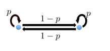
Such a system has of the form:
| (4) |
where . The eigenvalues of satisfy the equation
| (5) |
One solution comes from,
| (6) |
and the other from,
| (7) |
For the self loop is weaker than the edge connecting to the other node, and for the opposite is true. The spectral complexity is
| (8) |
Spectral complexity of this class of graphs distinguishes between graphs that have stronger self-interaction than interaction between the nodes, characterized by and the graphs in which the interaction between the nodes is stronger than the self-interaction. Note that spectral complexity is discontinuous at . This is in line with the behavior of the underlying Markov chain: for any initial probability distribution on the chain will decay exponentially and monotonically to the uniform distribution. For , the decay of the distribution assumes oscillatory manner, thus representing a qualitative, discontinuous change in behavior. Note that for the complexity measure shows features of a discrete metric. Thus, the discontinuity in the complexity metric accurately captures the transition from the more complex oscillatory evolution of the distribution to the invariant measure (for ) versus the less complex monotonic convergence to the invariant measure for . We note that the oscillatory nature of the distribution, in the more complex case, corresponds to strong interaction between nodes (since ). This is in contrast with the weak interactions between nodes in the case, whereby the graph interactions are less important when compared to the self interaction of nodes.
2.2 Physical intuition for complexity metric and meaning of eigenfunctions of the recurrence matrix for the network behavior
Spectral objects associated with undirected graphs -such as the Fiedler eigenvalue, that is associated with speed of mixing of the associated Markov chain and reflects connectivity of the underlying graph, and the Fiedler vector, whose components indicate subgraphs that have strong internal connectivity but weak interconnectivity - often have impact on the physical understanding of the network. The same is true for the eigenvalues and eigenvectors of the matrix . They have strong correlation with the structural properties of the underlying graph. For example, existence of a real eigenvalue indicates that the network can be split into two subnetworks that have weak internal connectivity but strong interconnectivity between two subnetworks (see Example 5). Also, the associated eigenvector values can be clustered into two separate sets that indicate the mentioned subgraphs. Both the simple example 5, and the large graph Wikipedia example in the section 4.2 provide evidence for this statement. Analogously, an eigenvalue set , whose arguments are close to indicates that the graph possesses 3 subgraphs with weak internal and strong connectivity between the 3 subgraphs. An example of this is shown in the section 4.2 for the Gnutella network.
The complexity metric has the above spectral elements as part of the metric. It speaks to the structural complexity of the graph, but it has a physical meaning for the behavior of the network as well. As a simple example, consider the case of spring mass system illustrated in figure 2. If we set , the weight matrix is
| (9) |
The associated recurrence matrix is then
| (10) |
where

Now assume . This indicates a decoupled system, and the complexity of such system is clearly the smallest among all considered systems. For slightly smaller then , the complexity is small, as the system is “almost decoupled”. For , the system has one eigenvalue at , indicating that the masses interact strongly, while there is no self-interaction for either mass. It is physically intuitive that the highest complexity occurs for , in which case the effects of both the spring attached to only one of the masses and the spring attached to both masses have equal influence on the individual mass motion. It is also intuitive that the situation with is less complex - for example, in design considerations we do not need to take into account the properties of two of the springs. This intuition carries over to other examples. If we take three masses with no self interaction, but connected by springs, there is a double eigenvalue at and thus its complexity is larger than that of the 2-mass system. The more balanced the self connectivity is with the connectivity to other nodes the more complex tasks like engineering design will become. It is sometimes argued that networks with full connectivity are simpler to analyze, but this comes from a statistical mechanics approach to the problem. In a design engineer or maintenance engineer world, adding an edge in the device or network design always increases the complexity of the resulting system.
The above discussion introduces a way of measuring the complexity of the recurrent part of a directed graph, and points to the intuitive aspects of the definition. But, complexity of the graph is not solely a function of the recurrence and cycles. Namely, more components in a graph, and more edges between non-recurrent nodes contribute to complexity as well - and we assume they do so in a linear fashion. Thus, if for a particular application we need to take into account the weights of nodes and the weights of the removed edges while removing sources, the total complexity can be formulated in the following way:
| (11) |
where is the user-defined weighting parameter for the spectral complexity in the total complexity metric that can take any value from . is the initial total number of nodes, ’s are the complexity of the individual nodes,333This is obtained either as user input or by some measure of complexity of dynamics on the individual node - e.g. through the use of the spectral distribution associated with the Koopman operator of the dynamical system [47]. is the number of edges removed while removing source nodes and ’s are the weights of the edges that were excluded in the source nodes removal step. is given by equation (1) and is the scaling factor that arises due to the fact that the terms and might have vastly different numerical values. One choice for is the following:
| (12) |
Note that the expectation is taken over various configurations of the system, and thus the probability distribution on a collection of graphs must be given. An alternative choice is to replace the operator with the nonlinear max operator in equation (12).
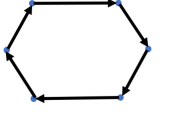
Example 6 (Unicyclic directed graphs)
Consider the family of unicyclic connected graphs, with nodes and edges , and (see figure 3). Let the complexity of individual nodes be , and . Then the complexity is equal to and increases monotonically with the size of the graph.
2.3 Comparison with Graph Energy
In this section, we compare the spectral complexity introduced in this paper to graph energy. The notion of graph energy [52, 53] emerged from molecular and quantum chemistry, where it has found use in ranking proteins on the basis of the level of folding [54]. It has also been used as a metric for complexity of graphs. The graph energy complexity, interestingly, does not peak for graphs with maximum possible connections (the rank of the adjacency matrix for a complete graph is not maximum). Instead, statistically the most complex graphs are those with possible connections [55]. Note that this complexity metric fails to capture directed cycles in the graph since one is forced to either work only with undirected or symmetrized directed graphs, as demonstrated below.
The algorithm for calculating graph energy is as follows. At first, for a given graph, we construct the adjacency matrix :
| (13) |
The graph energy is calculated by using the following formula:
| (14) |
where are edge weights, is the number of edges in the graph, is a vector of singular values of matrix . Equation (14) can be used with symmetrized adjacency matrix , where is the logical OR operator.
In the following, we present Figures 4 and 5 to highlight the difference between the complexity introduced in this paper and the graph energy. Random graphs were probabilistically constructed using the following formula: the probability with which a node is connected to another node is given by
All graphs considered have 1000 nodes. The average degree was varied from to in increments of and then from to in increments of . The degree is defined as the number of outgoing edges from each node. All weights of the edges are equal to 1. Each realization was repeated 10 times.
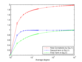
The spectral complexity increases fast with the average degree, reaching values of about 1.8 (out of the maximum possible value of 2) at an average degree of about 20/1000 of the total number of nodes; it then continues to increase monotonically, but less rapidly, with the average degree.
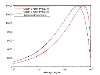
In the case of the graph energy, as shown in Figure 5, the maximum energy is reached when the average degree is at about 50% of the total number of nodes; then the graph energy starts to decrease.
This difference can be understood from the following argument. For simplicity, we take graphs with edge weights all equal to . As shown in Theorem 4, random graphs with large average degree will statistically have eigenvalues with modulus close to zero. Since graph energy is equal in this case to the sum of moduli of eigenvalues, the graph energy will be small. In other words, small graph energy is in fact indicative of a large number of connections in the graph, and thus large, not small, complexity. Namely, the key to decrease of energy of random graphs is the decrease in the moduli of the eigenvalues. In contrast, the metric F counts the number of complex eigenvalues, that will, in the case of a random graph with large average degree tend to increase with the average degree.
In the case of graphs corresponding to engineered systems, there is no reason why the complexity should decrease with increasing the number of connections (interdependencies) in the graph. Thus, we believe that the complexity measure introduced in this paper is more appropriate for engineering and physical systems. We note that the graph energy metric is more appropriate from an information theory standpoint.
We additionally note that in [56], the authors develop a complexity measure that is based on the entanglement of cycles in directed graphs. They compute this metric using a game theoretic approach (using a cops-and-robbers game). This reachability approach is similar in spirit to our spectral cyclomatic complexity measure. However, we note that, in general, computing -entanglements scales as , whereas our approach in general scales as , and much faster than that for sparse graphs. The spectral complexity captures the “entanglements” at all scales of the graph (for all ). Moreover, unlike the approach in [56], our methodology leads to natural clustering of the graph that is discussed in the next section.
3 Clustering of Directed Graphs
The clustering of undirected graphs is a well-developed area [5, 6, 7] with several decades of research behind it. The area of clustering of directed graphs is far less developed. However, the analysis and clustering of directed graphs is slowly coming in vogue [57, 36, 58, 59]. In [36], the author generalizes random walk based Cheeger bounds to directed graphs. These bounds are related to the spectral cuts often used for graph partitioning [5]. In [57], the authors generalize Laplacian dynamics to directed graphs, resulting in a modularity (quality) cost function for optimal splitting.
An alternative approach has focused on block modeling [58, 59]. Under this methodology, nodes are grouped into classes that exist in an image graph. This assignment is performed based on node connectivity and neighbor properties. This approach assumes that a template image graph and roles (for the nodes) are supplied a priori. The graph is then fit onto the image graph using an optimization scheme [58]. Although the approach extends to directed graphs, such image graphs are not always available in engineering or social systems.
In the following, we introduce a new graph clustering approach that complements standard spectral methods for decomposing graphs. In particular, we construct a new algorithm that is based on computing the underlying cycles in the graph by computing the corresponding generating eigenvalues and eigenvectors. In particular, by decomposing the graph into these cycles, we aim to identify strongly interacting components in a directed graph. The method is compared to Cheeger and Laplacian dynamic based methods [36, 57].
From the discussion leading to Theorem 1, we recognize that cycling in a directed graph is associated with its recurrent part. Thus, we can use spectral properties – and in particular complex eigenvalue pairs – of the recurrence matrix in order to recognize cycles in a directed graph. Note that, according to Theorem 1, a set of complex eigenvalues with unit modulus always has a generator . We extend this idea to eigenvalues off the unit circle and search for such generating eigenvalues.
In our algorithm, we seek the dominant cycle in a graph by identifying an eigenvalue (the generating eigenvalue) that is closest to a pure cycle on the unit circle. The algorithm is as follows: we compute nonzero eigenvalues of . We then compute the angles of the calculated eigenvalues in the complex plane and set
| (15) |
where , is the number of nonzero eigenvalues, is the set of eigenvalues for which . If the set is empty, then the minimum in equation (15) is 1. We denote the number of clusters corresponding to the dominant cycle as . Then we find the generating eigenvalue(s) and the corresponding eigenvector(s). We choose such that . We want the generating eigenvalue to be close to the case of a pure cycle of size , when the generating eigenvalue is at . We find the index of the first generating eigenvector as . Other generating eigenvalues are those that are within a predefined threshold (we use in our work) of the first generating eigenvalue.
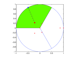
For each generating eigenvector we compute angles in the range for each element . Then we obtain graph clusters by partitioning coordinates of into groups by splitting the unit circle into equal parts. Disconnected nodes and sinks are placed in separate clusters.
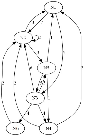
For example, the node graph (see Fig. 6 (left)) with non-zero eigenvalues of the recurrence matrix (red points in Fig. 6 (right)) has clusters. The sector of the unit circle, that contains the generating eigenvalue is between and and is colored with green in Fig. 6 (right). The generating eigenvalue is the non-zero eigenvalue which is closest to the eigenvalue of the pure cycle of size .
In previous work [60, 61] a method for identifying coarse-grained dynamics using aggregation of variables or states in linear dynamical systems was developed. The condition for aggregation is expressed as a permutation symmetry of a set of dual eigenvectors of the matrix that defines the dynamics. It is based on the fact that the aggregation matrix reduces a (transition) matrix P describing a linear dynamical system if and only if there exists a set of linearly independent vectors invariant under , e.g. (left) eigenvectors, that respect the same permutation symmetry group as . It is straightforward to identify permutation symmetries in the invariant vectors of . A permutation symmetry is realized through identical elements in the vectors. Thus, by identifying the above permutation symmetries, one can group elements in a complex (directed) graph. In other words, the algorithm that we introduced above leads to a natural method for graph sparsification [19].
4 Examples
4.1 Fixed Wing Aircraft Example
To test both our clustering approach and the complexity metric, we consider the architecture of a fixed wing aeroplane system [33]. This is a particularly important and relevant example since recent analysis by the RAND Corporation concluded that the increase in cost of fixed wing aircraft is primarily due to increased complexity [62]. An example of the impact of the complexity of fixed wing aircraft is the recent cost overruns of the F-35 platform [3].
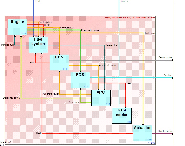
The aerospace system considered in this work, consists of the following functional subsystems: aircraft engine, fuel system, electrical power system (EPS), environmental control system (ECS), auxiliary power unit (APU), ram cooler, and actuation systems. These subsystems may be connected to one another through various means. For example, the engine may provide shaft power to the fuel system, the EPS and actuation system. Similarly, the APU may be connected to the engine as it may be required to provide start up pneumatic power. Note that the interconnections need not be electrical or mechanical in nature. Since the fuel system can be designed to absorb heat from the actuation system and EPS, the dependencies of the subsystems may also be thermal. For a discussion on these systems we refer the reader to [33]. An example architecture depicting the subsystems and their interconnections is shown in Fig. 7.
Traditionally, aerospace system architectures are specified by subsystems (such as EPS, ECS etc) and their interconnections. The exploration of design space for these aerospace systems can be a particularly daunting and challenging task. One possible approach to this problem has been to enumerate all feasible architectures and then pick the most desirable one [33]. It would appear that the exponential size of the design space would make this enumeration task intractable. However, the feasible set is typically very sparse and generative filters can be used to enumerate all the possible system designs [33].
In generative filters, one starts by defining the functional subsystems and then listing their interconnection rules. Based on these rules one can efficiently identify all possible architectures [33]. Using generative filtering on the fixed wing aircraft system gives feasible architectures (significantly less than the possible combinations of subsystem interconnection). One can now analyze and rank the resulting architectures based on complexity and interdependencies.
After analyzing 27,225 configurations of a system, we show the most complex one and the least complex one, from the definition of metrics in equation (1) and equation (11) with . We compare results obtained by using our spectral complexity with those obtained by using graph energy.
We compare our clustering results, with those obtained by using the Fiedler method, Cheeger bounds [36], and modularity maximization [57]. Our approach for the Fiedler method is as follows: at first for a given graph we construct the adjacency matrix according to equation (13). Then we symmetrize the obtained matrix as , where is the logical OR operator. After that we find the Laplacian matrix , where is the degree matrix. In this matrix, rows sum to zero. The Fiedler approach is based on the second smallest eigenvalue and the corresponding eigenvector of the symmetric matrix . In particular, the signs of the components of the corresponding eigenvector are used to partition the graph in two parts.
In the following, N1 will correspond to the engine, N2 to the fuel system, N3 to the EPS, N4 to the ECS, N5 to the APU, N6 to the ram cooler, and N7 to the actuation system.
4.1.1 High Complexity Architecture
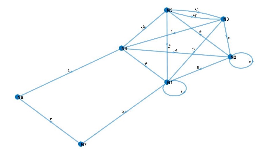
After analyzing all 27,255 configurations, the architecture number in Fig. 8 was found to be the most complex. The eigenvalues for the graph are displayed in Fig. 9.
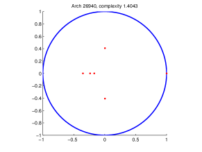
The complexity for this graph by using equation (1) and in equation (11) is equal to 1.4043. The complexity for the random graph with the same number of nodes and average degree by using equation (1) and in equation (11) is equal to 0.9237. The complexity predicted by equation (1) for the high complexity graph is about 152% of the value of complexity predicted in expectation by the same equation for a random graph. The complexity for this graph by using equation (1) and in equation (11) is equal to 1.2012.
The above complexity can be motivated from a “system cycle” standpoint. In particular, in Fig. 8 the cycles are,
-
1.
Fuel System Fuel System (self-loop)
-
2.
Engine Fuel System Engine
-
3.
Engine Fuel System APU Engine
-
4.
Fuel System APU EPS Fuel System
-
5.
Fuel System APU EPS Ram Cooler Fuel System
-
6.
Fuel System APU EPS ECS Engine.
These cycles capture energy, fuel, and data flows and interactions. We note that increased interactions amongst aircraft subsystems can be related to reduced efficiencies and failures [63]. Thus, multiple intersecting cycles with several nodes give rise to higher complexity systems since failure in single subsystems would propagate through the cycles and across thereby requiring additional redundancies for safety.
The nodes form the following clusters: cluster 1 contains Nodes 1 (engine), 4 (ECS), and 6 (ram cooler); cluster 2 is Node 2 (fuel system), cluster 3 is Node 3 (EPS); and cluster 4 is Node 5 (APU). Here we note that the single node clusters are ones that co-occur in multiple cycles. By visual inspection one can see the “leaky” (in the sense that eigenvalues corresponding to it are at a large distance from the unit circle) 4-cycle composed of the clusters; the system cycles through the 4-cycle giving rise to high complexity. This leakiness naturally arises due to the interactions of the various cycles (enumerated above) at common nodes such as Fuel System, APU etc.
The energy for this graph by using equation (14) is equal to 28.3401 (sum of singular values is equal to 7.9352). If the matrix is symmetrized, then the energy for this graph by using equation (14) is equal to 33.9041 (sum of singular values is equal to 9.4931).
By using the Fiedler method the graph is divided into the following clusters: cluster 1 contains Nodes 2 (fuel system), 3 (EPS) and 6 (ram cooler); cluster 2 contains Nodes 1 (engine), 4 (ECS) and 5 (APU), which neither captures strongly connected components nor critical nodes that co-occur in multiple cycles.
Using a Cheeger bound approach [36], we find that the above graph is split into two groups. Cluster 1 contains nodes and cluster 2 contains nodes . The spectral approach for modularity maximization (by analyzing the leading eigenvector) yields a clustering where nodes are in the first cluster and nodes lie in cluster 2. Neither of these methods capture the visually evident cycling behavior. We now contrast this architecture with one of low complexity as identified by our approach.
4.1.2 Low Complexity Architecture
After analyzing all 27,255 configurations as above, the architecture number in Fig. 10 was found to be the least complex, not counting very simple graphs containing mostly disjoint nodes after removing sources. The eigenvalues for the graph are displayed in Fig. 11.

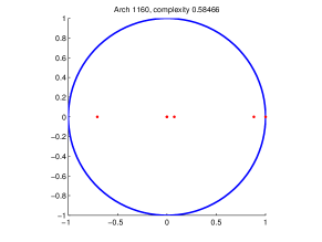
The complexity by using equation (1) and in equation (11) is equal to 0.5847. The complexity for the random graph with the same number of nodes and average degree by using equation (1) and in equation (11) is equal to 0.8136. The complexity predicted by equation (1) for the low complexity graph is about 71% of the value of complexity predicted in expectation by the same equation for a random graph. The complexity by using equation (1) and in equation (11) is equal to 0.8195.
As in the previous case, the complexity can again be motivated from a “system cycle” standpoint. In particular, in Fig. 8 the cycles are,
-
1.
Fuel System Fuel System (self-loop)
-
2.
Engine Fuel System Engine
-
3.
Engine EPS Engine
-
4.
APU EPS APU
-
5.
Fuel System APU EPS Fuel System.
Compared to the architecture with higher complexity, we see that this example has only cycles versus in the previous one. Additionally, the cycles in the higher complexity architecture have more nodes (hops) when compared to the low complexity architecture. Thus, the previous architecture had a higher complexity when compared to the current one despite the fact that the current example has one additional node (7 nodes) when compared to the previous one (6 nodes).
The nodes form the following clusters: cluster 1 contains Nodes 1 (engine) and 5 (APU); cluster 2 contains Nodes 2 (fuel system) and 3 (EPS). It is easy to check that these nodes generate the cycles in the graph. The eigenvalues indicate a “leaky” two cycle with these two clusters. Nodes 4 (ECS), 6 (ram cooler) and 7 (actuation systems) are sinks. These unidirectional connections lower the complexity of the system.
The energy for this graph by using equation (14) is equal to 25.6040 (sum of SVDs is equal to 7.2359). If the matrix is symmetrized, then the energy for this graph by using equation (14) is equal to 34.8340 (sum of SVDs is equal to 9.8444). Thus, in contrast to spectral complexity, they are not much different in values obtained for the high complexity architecture. Note that the self loop of node 2 is not included in the energy calculation.
Using a Cheeger bound approach [36], we find that the clustering approach finds no partition. The spectral approach for modularity maximization (by analyzing the leading eigenvector) and Fiedler method both yield a clustering where nodes are in the first cluster and nodes lie in cluster . Once again, these methods do not capture the cycling behavior.
4.2 Large Network Examples
In this subsection we provide examples of calculating complexity and clustering for some large graphs.
4.2.1 Wikipedia who-votes-on-whom network
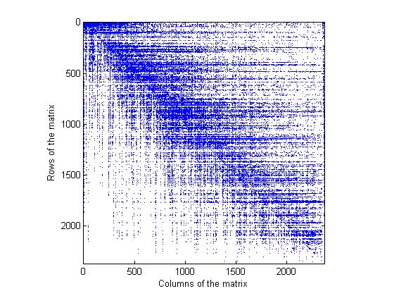
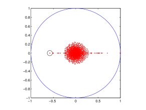
At first we consider the Wikipedia who-votes-on-whom network with nodes ([34]). Nodes in the network represent Wikipedia users and a directed edge from node to node represents that user voted for user . After removing sources, the network has 2,372 nodes. This is to be expected since most nodes are simply voters that do not compete in elections (making them sources with no incoming edges). In Figure 12, we show nonzero elements of the recurrence matrix. The multiplicity of is and the multiplicity of is , which corresponds to 42.4% of the total number of nodes. In Figure 13, we show all non-zero eigenvalues of the recurrence matrix.
Complexity
The complexity obtained from equation (1) is equal to 1.0418 (0.4938+0.5480). The complexity for the random graph with the same number of nodes and average degree by using equation (1) is equal to 1.8171 (0.8215+0.9956). The complexity predicted by equation (1) for the Wikipedia who-votes-on-whom graph is about 57% of the value of complexity predicted by the same equation for the random graph, indicating an internal structure to the graph. Looking at the eigenvalue distribution shown in figure 13, we see that it has the structure of randomly distributed eigenvalues inside a disk of small radius. We know from theorem 3 that such distributions of eigenvalues yield high spectral complexity. There is also a set of eigenvalues away from that disk on positive and negative real line inside the unit disc. We next show, using clustering, that there is internal structure corresponding to a low period – namely period 2-cycle that contributes to an eigenvalue on the negative real line that lowers complexity over the maximally complex graph, or even a random graph.
Clustering
There are disjoint single nodes for Wikipedia who-votes-on-whom network which are not considered for clustering. The graph contains 1,016 sinks. The clustering was done for the strongly connected component. We obtained cluster C1 of nodes and cluster C2 of nodes. The generating eigenvalue is -0.5792588, indicating a 2-cycle.
In Figure 14, we plot the ratio of the number of edges going from cluster X to cluster Y to the number of edges inside cluster X depending on the percentage of nodes in all clusters. The percentage of nodes in all clusters is calculated as follows: we first sort the generating eigenvector in the ascending order. We then compute the fraction of nodes to keep such that the sum of the ratios is the maximum.
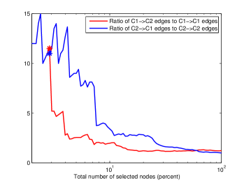
In the following, we select such percentage of nodes in all clusters so that the sum of two ratios, plotted as solid lines in Figure 14, is the maximum. We mark the found point of 2.9% with on Figure 14. The obtained graph is shown in Figure 15, where nodes’ numbers are numbers in the graph before removing sources. The number of nodes in each cluster and the ratio of the number of edges between clusters or inside the cluster to the number of nodes in the cluster are shown in Table 1. The average degree of this graph is , calculated as the ratio of the total number of outgoing edges from each cluster and edges inside each cluster to the total number of nodes in clusters. In the table, the number in parenthesis shows the number of nodes in the corresponding cluster. Other numbers show the ratio of the number of edges from X to Y to the number of nodes in X, where X can be cluster C1 and cluster C2 and Y can be cluster C1 and cluster C2. As it can be seen from the table the biggest ratio is for C1 to C2 and for C2 to C1.
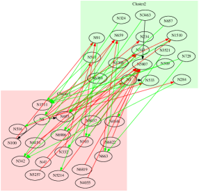
| X | XC1 | XC2 |
|---|---|---|
| C1 (19) | 0.1053 | 1.2105 |
| C2 (18) | 1.2222 | 0.1111 |
The number of nodes in each cluster and the ratio of the number of edges between clusters or inside the cluster to the number of nodes in the cluster in the case of 100% of initial number of nodes in all clusters are shown in Table 2. The average degree is 30.3508. As it can be seen from the table the biggest ratio is for C1 to C2.
| X | XC1 | XC2 |
|---|---|---|
| C1 (622) | 14.2910 | 17.5595 |
| C2 (678) | 14.4130 | 14.5619 |
We also performed clustering for the strongly connected component by using the Fiedler method. We obtained cluster 1 of 1,280 nodes and cluster 2 of 20 nodes (a highly unbalanced cut). The table for the number of nodes in each cluster and the ratio of the number of edges between clusters or inside the cluster to the number of nodes in the cluster are shown in Table 3. The number of edges between and inside clusters is calculated for the directed graph before the symmetrization of the adjacency matrix. The smallest ratio is for C1 to C2, what reveals the weak connection from C1 to C2. We see that the method is not capable of uncovering any strong internal structure in this directed graph.
| X | XC1 | XC2 |
|---|---|---|
| C1 (1280) | 29.7891 | 0.5398 |
| C2 (20) | 29.600 | 2.1500 |
4.2.2 Gnutella peer to peer network
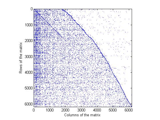
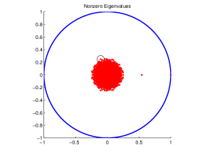
In the following, we consider the Gnutella peer to peer network with nodes ([34]). Nodes represent hosts in the Gnutella network topology and edges represent connections between the Gnutella hosts. After removing sources the network has 6,179 nodes. In Figure 16, we show nonzero elements of the recurrence matrix. There are 674 zero eigenvalues and 3,836 one eigenvalues, which are 62.0% of the total number of nodes. In Figure 17, we show all non-zero eigenvalues of the matrix. We again see the structure similar to the Wikipedia network, but with even stronger indication of complexity indicated by the concentration of eigenvalues inside the disk of small radius. The eigenvector corresponding to the eigenvalue of about 0.5 has zero components for sinks and the same sign nonzero components for nodes that are not sinks.
Complexity
The complexity by using equation (1) is equal to . The complexity for the random graph with the same number of nodes and average degree by using equation (1) is equal to 1.5522 (0.5976+0.9546). Thus, the complexity predicted by equation (1) for the Gnutella graph is about 36% of the value of complexity predicted by the same equation for the random graph, again indicating structure induced by a low-period cycle that we uncover next.
Clustering
There are disjoint single nodes in the Gnutella graph which are not considered for clustering. The graph contains 3,960 sinks. The clustering algorithm found the generating eigenvalue (see the circled eigenvalue in the figure 17). From the associated generating eigenvector we obtained three clusters: cluster C1 of nodes, cluster C2 of nodes, cluster C3 of nodes.
In Figure 18 we plot the ratio of the number of edges going from cluster X to cluster Y to the number of edges inside cluster X depending on the percentage of nodes in all clusters.
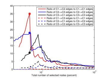
In the following, we select such percentage of nodes in all clusters so that the sum of three ratios, plotted as solid lines in Figure 18, is the maximum. We mark the found point of 6.0% with on Figure 18. After removal of nodes that become disjoint when the clusters were reduced in size this percentage is 4.6. The obtained graph is shown in Figure 19, where nodes’ numbers are numbers in the graph before removing sources. The number of nodes in each cluster and the ratio of the number of edges between clusters or inside the cluster to the number of nodes in the cluster are shown in Table 4. The average degree of this graph is 0.9263. As it can be seen from the table the biggest ratios are for C1 C2, C2 C3, C3 C1.
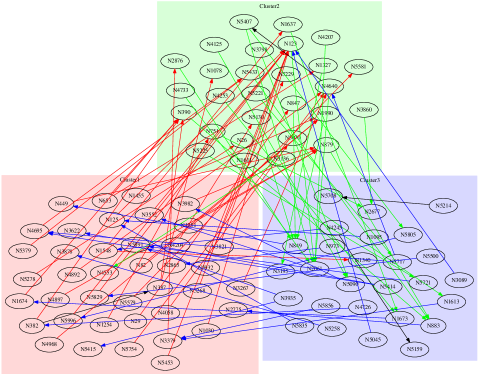
| X | XC1 | XC2 | XC3 |
|---|---|---|---|
| C1 (40) | 0.0250 | 0.8750 | 0.0250 |
| C2 (28) | 0.0357 | 0.0357 | 0.8214 |
| C3 (27) | 0.7778 | 0.1111 | 0.0741 |
The number of nodes in each cluster and the ratio of the number of edges between clusters or inside the cluster to the number of nodes in the cluster in the case of 100% are shown in Table 5. The average degree of this graph is 4.5034. As it can be seen from the table the biggest ratios are for C1 C2, C2 C3, C3 C1, but the ratio between them and other elements of the matrix is smaller than in the 6% case.
| X | XC1 | XC2 | XC3 |
|---|---|---|---|
| C1 (659) | 1.1153 | 2.3505 | 1.2337 |
| C2 (675) | 0.9052 | 1.1037 | 2.2504 |
| C3 (734) | 2.0763 | 1.1662 | 1.3093 |
The clustering of the strongly connected component by using the Fiedler method gives cluster 1 of 1,878 nodes and cluster 2 of 190 nodes. The number of nodes in each cluster and the ratio of the number of edges between clusters or inside the cluster to the number of nodes in the cluster are shown in Table 6. The number of edges between and inside clusters is calculated for the directed graph before the symmetrization of the adjacency matrix. As it can be seen from the table the smallest ratio is for C1 to C2, what reveals the weak connection from C1 to C2. Again, the method fails to uncover the internal structure in the graph because the structure is of cycling type, and not of separate subgraph type.
| X | XC1 | XC2 |
|---|---|---|
| C1 (1878) | 4.3679 | 0.2023 |
| C2 (190) | 2.5632 | 1.2789 |
5 Conclusions
In this work we proposed a new, spectral, measure of complexity of systems and an associated spectral clustering algorithm. This complexity measure (that we call spectral complexity) is based on the spectrum of the underlying interconnection graph of the subcomponents in the system. Spectral complexity is a natural engineering extension to software complexity measures developed in [9]. We find that compared to competing complexity measures (such as graph energy), spectral complexity is more appropriate for engineering systems. For example, one of its features is that the complexity monotonically increases with the average node degree. In addition, it properly accounts for structure and complexity features induced by cycles in a directed graph. Using the spectral complexity measure, comparison of complex engineered systems is enabled, potentially providing significant savings in design and testing.
Spectral complexity also provides an intuitive approach for clustering directed graphs. It partitions the graph into subgroups that map into one another. Our partitioning shows a strong cycling structure even for complex networks such as Wikipedia and Gnutella, that the standard methodologies like the Fiedler vector partitioning do not provide.
Our methods are demonstrated on engineering systems, random graphs, Wikipedia and Gnutella examples. We find that the high and low spectral complexity architectures uncovered by our methods correspond to an engineer’s intuition of a highly complex vs. a low complexity architecture. Namely, the low complexity of the engineered architecture is related to more layers in its horizontal-vertical decomposition [45, 64] i.e. with a graph structure closer to acyclic.
It is of interest to note that the methods introduced here have proven to be of strong use in data-driven analysis of dynamical systems [65], which should make it possible to combine the introduced measure of complexity with measure of dynamic complexity for dynamical systems on networks.
6 Acknowledgements
We are thankful to an anonymous referee for comments that vastly improved the presentation of the material over the original version. The views expressed are those of the author and do not reflect the official policy or position of the Department of Defense or the U.S. Government. Approved for Public Release, Distribution Unlimited.
This work was partially supported under AFOSR grant FA9550-17-C-0012 and under DARPA Contract FA8650-10-C-7080.
The authors thank the anonymous reviewers for their insightful feedback and suggestions.
References
- [1] Steven D Eppinger and Tyson R Browning. Design structure matrix methods and applications. MIT press, 2012.
- [2] Antonio Pugliese, James Enos, and Roshanak Nilchiani. Acquisition and development programs through the lens of system complexity. 2018.
- [3] Drew Robbins, John Bobalik, David De Stena, Nick Martin, Ken Plag, Keith Rail, and Ken Wall. F-35 subsystems design, development & verification. In 2018 Aviation Technology, Integration, and Operations Conference, page 3518, 2018.
- [4] Dragoš M Cvetković, Michael Doob, and Horst Sachs. Spectra of graphs: theory and application, volume 87. Academic Pr, 1980.
- [5] Fan RK Chung and Fan Chung Graham. Spectral graph theory. Number 92. American Mathematical Soc., 1997.
- [6] Ulrike Von Luxburg. A tutorial on spectral clustering. Statistics and computing, 17(4):395–416, 2007.
- [7] Tuhin Sahai, Alberto Speranzon, and Andrzej Banaszuk. Hearing the clusters of a graph: A distributed algorithm. Automatica, 48(1):15–24, 2012.
- [8] Stefan Klus and Tuhin Sahai. A spectral assignment approach for the graph isomorphism problem. Information and Inference: A Journal of the IMA, 2018.
- [9] Thomas J McCabe. A complexity measure. IEEE Transactions on software Engineering, (4):308–320, 1976.
- [10] Thomas J McCabe and Charles W Butler. Design complexity measurement and testing. Communications of the ACM, 32(12):1415–1425, 1989.
- [11] Jainendra K. Navlakha. A survey of system complexity metrics. The Computer Journal, 30(3):233–238, 1987.
- [12] Martin Shepperd and Darrel C Ince. A critique of three metrics. Journal of Systems and Software, 26(3):197–210, 1994.
- [13] Karl Johan Aström and Richard M Murray. Feedback systems: an introduction for scientists and engineers. Princeton university press, 2010.
- [14] Thilo Moshagen. Convergence of explicitely coupled simulation tools (co-simulations). Journal of Numerical Mathematics, 2017.
- [15] Stefan Klus, Tuhin Sahai, Cong Liu, and Michael Dellnitz. An efficient algorithm for the parallel solution of high-dimensional differential equations. Journal of computational and applied mathematics, 235(9):3053–3062, 2011.
- [16] Matthias Dehmer and Abbe Mowshowitz. A history of graph entropy measures. Information Sciences, 181(1):57–78, 2011.
- [17] Matthias Dehmer, Xueliang Li, and Yongtang Shi. Connections between generalized graph entropies and graph energy. Complexity, 21(1):35–41, 2015.
- [18] Igor Mezić and Thordur Runolfsson. Uncertainty propagation in dynamical systems. Automatica, 44(12):3003–3013, 2008.
- [19] Michael B Cohen, Jonathan Kelner, John Peebles, Richard Peng, Anup B Rao, Aaron Sidford, and Adrian Vladu. Almost-linear-time algorithms for Markov chains and new spectral primitives for directed graphs. In Proceedings of the 49th Annual ACM SIGACT Symposium on Theory of Computing, pages 410–419. ACM, 2017.
- [20] Conrad Kottak. Cultural anthropology. 5th ad. New York: Me—Graw Hil1, 1991.
- [21] Nora Speer, Holger Frohlich, Christian Spieth, and Andreas Zell. Functional grouping of genes using spectral clustering and gene ontology. In Neural Networks, 2005. IJCNN’05. Proceedings. 2005 IEEE International Joint Conference on, volume 1, pages 298–303. IEEE, 2005.
- [22] Alberto Paccanaro, James A Casbon, and Mansoor AS Saqi. Spectral clustering of protein sequences. Nucleic acids research, 34(5):1571–1580, 2006.
- [23] Abubakr Muhammad and Ali Jadbabaie. Decentralized computation of homology groups in networks by gossip. In American Control Conference, 2007. ACC’07, pages 3438–3443. IEEE, 2007.
- [24] Ivan Herman, Guy Melançon, and M Scott Marshall. Graph visualization and navigation in information visualization: A survey. IEEE Transactions on visualization and computer graphics, 6(1):24–43, 2000.
- [25] David Kempe and Frank McSherry. A decentralized algorithm for spectral analysis. In Proceedings of the thirty-sixth annual ACM symposium on Theory of computing, pages 561–568. ACM, 2004.
- [26] Miroslav Fiedler. Algebraic connectivity of graphs. Czechoslovak mathematical journal, 23(2):298–305, 1973.
- [27] Miroslav Fiedler. A property of eigenvectors of nonnegative symmetric matrices and its application to graph theory. Czechoslovak Mathematical Journal, 25(4):619–633, 1975.
- [28] Norman Biggs, Norman Linstead Biggs, and Emeritus Norman Biggs. Algebraic graph theory, volume 67. Cambridge university press, 1993.
- [29] Brian Everitt, Sabine Landau, Morven Leese, and Daniel Stahl. Cluster analysis. 4th. Arnold, London, 2001.
- [30] Anil K Jain and Richard C Dubes. Algorithms for clustering data. 1988.
- [31] Tuhin Sahai, Alberto Speranzon, and Andrzej Banaszuk. Wave equation based algorithm for distributed eigenvector computation. In Decision and Control (CDC), 2010 49th IEEE Conference on, pages 7308–7315. IEEE, 2010.
- [32] Satu Elisa Schaeffer. Graph clustering. Computer science review, 1(1):27–64, 2007.
- [33] Lawrence Zeidner, Andrzej Banaszuk, and Sandor Becz. System complexity reduction via spectral graph partitioning to identify hierarchical modular clusters. In 10th AIAA Aviation Technology, Integration, and Operations (ATIO) Conference, page 9265, 2010.
- [34] Jure Leskovec and Andrej Krevl. SNAP Datasets:Stanford large network dataset collection. 2015.
- [35] Richard A Brualdi. Spectra of digraphs. Linear Algebra and its Applications, 432(9):2181–2213, 2010.
- [36] Fan Chung. Laplacians and the cheeger inequality for directed graphs. Annals of Combinatorics, 9(1):1–19, 2005.
- [37] David Gleich. Hierarchical directed spectral graph partitioning. Information Networks, 2006.
- [38] Andrea Capocci, Vito DP Servedio, Guido Caldarelli, and Francesca Colaiori. Detecting communities in large networks. Physica A: Statistical Mechanics and its Applications, 352(2-4):669–676, 2005.
- [39] Marina Meilă and William Pentney. Clustering by weighted cuts in directed graphs. In Proceedings of the 2007 SIAM international conference on data mining, pages 135–144. SIAM, 2007.
- [40] Elizabeth A Leicht and Mark EJ Newman. Community structure in directed networks. Physical review letters, 100(11):118703, 2008.
- [41] Hao Yin, Austin R Benson, Jure Leskovec, and David F Gleich. Local higher-order graph clustering. In Proceedings of the 23rd ACM SIGKDD International Conference on Knowledge Discovery and Data Mining, pages 555–564. ACM, 2017.
- [42] Hadrien Van Lierde, Tommy WS Chow, and Jean-Charles Delvenne. Spectral clustering algorithms for the detection of clusters in block-cyclic and block-acyclic graphs. Journal of Complex Networks, 2018.
- [43] Christine Klymko and Geoffrey Sanders. Detecting highly cyclic structure with complex eigenpairs. arXiv preprint arXiv:1609.05740, 2016.
- [44] Igor Mezic, Vladimir A Fonoberov, Maria Fonoberova, and Tuhin Sahai. Complexity and clustering metrics. DARPA METAII PI meeting, September 2011.
- [45] Igor Mezic. Coupled nonlinear dynamical systems: Asymptotic behavior and uncertainty propagation. In Decision and Control, 2004. CDC. 43rd IEEE Conference on, volume 2, pages 1778–1783. IEEE, 2004.
- [46] Bernard O Koopman. Hamiltonian systems and transformation in Hilbert space. Proceedings of the National Academy of Sciences, 17(5):315–318, 1931.
- [47] Igor Mezić and Andrzej Banaszuk. Comparison of systems with complex behavior. Physica D: Nonlinear Phenomena, 197(1-2):101–133, 2004.
- [48] Geoffrey Grimmett and David Stirzaker. Probability and random processes. Oxford university press, 2001.
- [49] Anatole Katok and Boris Hasselblatt. Introduction to the modern theory of dynamical systems, volume 54. Cambridge university press, 1997.
- [50] Wilhelm Huisinga and Bernd Schmidt. Advances in algorithms for macromolecular simulation, chapter metastability and dominant eigenvalues of transfer operators. Lecture Notes in Computational Science and Engineering. Springer, 2005.
- [51] Charles Bordenave, Pietro Caputo, and Djalil Chafaï. Circular law theorem for random Markov matrices. Probability Theory and Related Fields, 152(3-4):751–779, 2012.
- [52] I Gutman. The energy of a graph. 10. steiermrkisches mathematisches symposium (stift rein, graz, 1978). Ber. Math.-Statist. Sekt. Forsch. Graz, (100-105), 1978.
- [53] Ivan Gutman. The energy of a graph: old and new results. In Algebraic combinatorics and applications, pages 196–211. Springer, 2001.
- [54] Ernesto Estrada. Characterization of 3D molecular structure. Chemical Physics Letters, 319(5-6):713–718, 2000.
- [55] Ivan Gutman, Tanja Soldatović, and Dušica Vidović. The energy of a graph and its size dependence. a Monte Carlo approach. Chemical physics letters, 297(5-6):428–432, 1998.
- [56] Dietmar Berwanger, Erich Grädel, Łukasz Kaiser, and Roman Rabinovich. Entanglement and the Complexity of Directed Graphs. Theoretical Computer Science, 463(0):2–25, 2012. Special Issue on Theory and Applications of Graph Searching Problems.
- [57] Peter J Mucha, Thomas Richardson, Kevin Macon, Mason A Porter, and Jukka-Pekka Onnela. Community structure in time-dependent, multiscale, and multiplex networks. science, 328(5980):876–878, 2010.
- [58] Jörg Reichardt and Douglas R White. Role models for complex networks. The European Physical Journal B, 60(2):217–224, 2007.
- [59] Brian Karrer and Mark EJ Newman. Stochastic blockmodels and community structure in networks. Physical review E, 83(1):016107, 2011.
- [60] Martin Nilsson Jacobi and Olof Görnerup. A spectral method for aggregating variables in linear dynamical systems with application to cellular automata renormalization. Advances in Complex Systems, 12(02):131–155, 2009.
- [61] Martin Nilsson Jacobi and Olof Goernerup. A dual eigenvector condition for strong lumpability of Markov chains. arXiv preprint arXiv:0710.1986, 2007.
- [62] Mark V Arena, Obaid Younossi, Kevin Brancato, Irv Blickstein, and Clifford A Grammich. Why has the cost of fixed-wing aircraft risen? a macroscopic examination of the trends in us military aircraft costs over the past several decades. Technical report, RAND NATIONAL DEFENSE RESEARCH INST SANTA MONICA CA, 2008.
- [63] JA Rosero, JA Ortega, E Aldabas, and LARL Romeral. Moving towards a more electric aircraft. IEEE Aerospace and Electronic Systems Magazine, 22(3):3–9, 2007.
- [64] Jianfeng Xu and Yueheng Lan. Hierarchical feedback modules and reaction hubs in cell signaling networks. PLOS ONE, 10(5):e0125886, 2015.
- [65] Marko Budišić, Ryan Mohr, and Igor Mezić. Applied Koopmanism. Chaos: An Interdisciplinary Journal of Nonlinear Science, 22(4):047510, 2012.