The Impact of Wrong Assumptions in BAO Reconstruction

Blake D. Sherwin    Martin White
Abstract

The process of density field reconstruction enhances the statistical power of distance scale measurements using baryon acoustic oscillations (BAO). During this process a fiducial cosmology is assumed in order to convert sky coordinates and redshifts into distances; fiducial bias and redshift-space-distortion parameters are also assumed in this procedure. We analytically assess the impact of incorrect cosmology and bias assumptions on the post-reconstruction power spectra using low-order Lagrangian perturbation theory, deriving general expressions for the incorrectly reconstructed spectra. We find that the BAO peak location appears to shift only by a negligible amount due to wrong assumptions made during reconstruction. However, the shape of the BAO peak and the quadrupole amplitude can be affected by such errors (at the percent- and five-percent-level respectively), which potentially could cause small biases in parameter inference for future surveys; we outline solutions to such complications.

1 Introduction

The measurement of baryon acoustic oscillations in the clustering of galaxies and the intergalactic medium provides some of our tightest constraints on the cosmological distance scale (for a review of recent measurements see [1], e.g. Fig. 14, for reviews of the methods see [2, 3]). With the exception of the intergalactic medium results, all recent measurements have employed a process known as “reconstruction” [4], which aims to undo some of the loss of signal due to non-linear evolution by estimating the motion of tracers under gravity and reversing it. In order to perform reconstruction, one typically assumes a fiducial cosmology to convert sky positions and redshifts into comoving coordinates; one also assumes a fiducial bias and redshift-space distortion (RSD) parameter to derive the density field from the galaxy distribution. However, the cosmology assumed may not match the true, underlying cosmology, and the fiducial bias and RSD parameters may also not equal their true values. In this paper we use Lagrangian perturbation theory to assess the impact of such errors in the assumed cosmology, biasing and RSD upon the two-point clustering of the reconstructed field.

Reconstruction has been extensively studied in the literature using both N-body simulations and analytic models [4, 5, 6, 7, 8, 9, 10, 11, 12, 13, 14, 15, 16, 17, 18, 19, 20]. While the impact of incorrect choices of distance, growth rate and bias has been studied in numerical simulations in particular cases, we are not aware of any analytic treatment. Since the standard algorithm is based upon the Zel’dovich approximation [21], we choose to similarly use low-order Lagrangian perturbation theory to assess the impact of incorrect assumptions about the cosmological model upon the recovered statistics. While the results will only be approximate, due to our approximate model of structure formation, they allow us to provide general formulae and hence estimate the errors introduced in any scenario.

The outline of the paper is as follows. In Section 2 we briefly review Lagrangian perturbation theory and reconstruction and define our notation. Section 3 explains the calculation of the reconstructed power spectra in a simple case where only the assumed distances are incorrect. Section 4 describes the more general calculation where the distances, the growth rate and the bias assumed can all be wrong. In Section 5, we evaluate our calculations and discuss the results. We conclude in Section 6.

2 Background

This section reviews material which has been extensively discussed in the literature already and is included primarily to set notation and present some results which will be of use later.

We choose to study reconstruction within the framework of Lagrangian perturbation theory (largely following Refs. [22, 23]). Lagrangian theory describes the evolution of large scale structure as a mapping from the original positions of a fluid element, 𝐪𝐪{\bf q}, to the final position, 𝐱𝐱{\bf x}, via a displacement vector, 𝚿𝚿{\bf\Psi}. Mass conservation then implies that the Fourier-space mass density in Eulerian coordinates can be written

δ(𝐤)=d3qei𝐤𝐪(ei𝐤𝚿(𝐪)1).𝛿𝐤superscript𝑑3𝑞superscript𝑒𝑖𝐤𝐪superscript𝑒𝑖𝐤𝚿𝐪1\delta({\bf k})=\int d^{3}q\ e^{-i{\bf k}\cdot{\bf q}}\left(e^{-i{\bf k}\cdot{\bf\Psi}({\bf q})}-1\right). (2.1)

As a first step we will neglect bias and redshift-space distortions. The computation of the power spectrum, at lowest order in (resummed) Lagrangian perturbation theory, then follows a standard procedure [22, 23]. Let us quickly review the steps. We compute δ(𝐤1)δ(𝐤2)delimited-⟨⟩𝛿subscript𝐤1superscript𝛿subscript𝐤2\langle\delta({\bf k}_{1})\delta^{\star}({\bf k}_{2})\rangle and use the cumulant theorem to evaluate the expectation value of an exponential:

d3qe𝐤𝐪(ei[𝐤𝚿(𝐪1)𝐤𝚿(𝐪2)]1)d3qe𝐤𝐪(ek2Σ2/2exp[2kikjξij(q)]1),similar-to-or-equalssuperscript𝑑3𝑞superscript𝑒𝐤𝐪delimited-⟨⟩superscript𝑒𝑖delimited-[]𝐤𝚿subscript𝐪1𝐤𝚿subscript𝐪21superscript𝑑3𝑞superscript𝑒𝐤𝐪superscript𝑒superscript𝑘2superscriptΣ222subscript𝑘𝑖subscript𝑘𝑗subscript𝜉𝑖𝑗𝑞1\int d^{3}qe^{-{\bf k}\cdot{\bf q}}\left(\left\langle e^{-i\left[{\bf k}\cdot{\bf\Psi}({\bf q}_{1})-{\bf k}\cdot{\bf\Psi}({\bf q}_{2})\right]}\right\rangle-1\right)\simeq\int d^{3}qe^{-{\bf k}\cdot{\bf q}}\left(e^{-k^{2}\Sigma^{2}/2}\exp\left[2\,k_{i}k_{j}\xi_{ij}(q)\right]-1\right), (2.2)

where q=|𝐪1𝐪2|𝑞subscript𝐪1subscript𝐪2q=\left|{\bf q}_{1}-{\bf q}_{2}\right|, ξij(q)=Ψi(𝐪1)Ψj(𝐪2)subscript𝜉𝑖𝑗𝑞delimited-⟨⟩subscriptΨ𝑖subscript𝐪1subscriptΨ𝑗subscript𝐪2\xi_{ij}(q)=\left\langle\Psi_{i}({\bf q}_{1})\Psi_{j}({\bf q}_{2})\right\rangle is the Lagrangian 2-point function and we have defined

Σ2=dk3π2PL(k).superscriptΣ2𝑑𝑘3superscript𝜋2subscript𝑃𝐿𝑘\Sigma^{2}=\int\frac{dk}{3\pi^{2}}\ P_{L}(k). (2.3)

We caution the reader that there are other definitions of Σ2superscriptΣ2\Sigma^{2} in the literature, differing by factors of 2. Expanding111Expanding the non-zero-lag piece of the correlator from the exponential while keeping the zero-lag (Σ2superscriptΣ2\Sigma^{2}) terms exponentiated is a reasonable approximation on large scales for CDM cosmologies, but can be problematic in general. See discussion in Refs. [24, 25, 16]. the second, non-zero-lag (i.e., 𝐪1𝐪2subscript𝐪1subscript𝐪2{\bf q}_{1}\neq{\bf q}_{2}) exponential in Eq. (2.2) to linear order in the ξijsubscript𝜉𝑖𝑗\xi_{ij} and dropping a constant term, the Fourier transform is simply the linear power spectrum PL(k)subscript𝑃𝐿𝑘P_{L}(k). We thus obtain P(k)=ek2Σ2/2PL(k)+𝑃𝑘superscript𝑒superscript𝑘2superscriptΣ22subscript𝑃𝐿𝑘P(k)=e^{-k^{2}\Sigma^{2}/2}\ P_{L}(k)+\cdots. This result reveals the well known fact that features in the power spectrum, such as the baryon acoustic oscillations, are damped by non-linear structure formation222In configuration space, the peak in the correlation function is convolved with a Gaussian of width ΣΣ\Sigma and thus broadened. [26]. Had we kept higher order terms (the \cdots), they would have included mode coupling terms which give a slight shift to the oscillations in the power spectrum or the location of the peak in the correlation function. These mode coupling terms are small, and they will be further multiplied by small factors of order the fractional errors in cosmology, bias and RSD; we will therefore neglect them in what follows.

Continuing to neglect bias and redshift-space distortions, the standard reconstruction algorithm [4] works as follows: we smooth the density field with a filter, S(k)𝑆𝑘S(k), to remove small scale modes and compute the negative Zel’dovich displacement

𝐬(𝐤)i𝐤k2S(k)δ(𝐤)𝐬𝐤𝑖𝐤superscript𝑘2𝑆𝑘𝛿𝐤{\bf s}({\bf k})\equiv-i\frac{{\bf k}}{k^{2}}\ S(k)\delta({\bf k}) (2.4)

The typical choice for the filter function, S(k)𝑆𝑘S(k), is a Gaussian. We then displace the original density field tracers by this vector to give the “displaced field”

δd(𝐤)=d3qei𝐤𝐪(ei𝐤[𝚿(𝐪)+𝐬(𝐪)]1).subscript𝛿𝑑𝐤superscript𝑑3𝑞superscript𝑒𝑖𝐤𝐪superscript𝑒𝑖𝐤delimited-[]𝚿𝐪𝐬𝐪1\delta_{d}({\bf k})=\int d^{3}q\ e^{-i{\bf k}\cdot{\bf q}}\left(e^{-i{\bf k}\cdot\left[{\bf\Psi}({\bf q})+{\bf s}({\bf q})\right]}-1\right). (2.5)

We also displace a random set of particles by the same amount to give the “shifted field”:

δs(𝐤)=d3qei𝐤𝐪(ei𝐤[𝐬(𝐪)]1)subscript𝛿𝑠𝐤superscript𝑑3𝑞superscript𝑒𝑖𝐤𝐪superscript𝑒𝑖𝐤delimited-[]𝐬𝐪1\delta_{s}({\bf k})=\int d^{3}q\ e^{-i{\bf k}\cdot{\bf q}}\left(e^{-i{\bf k}\cdot\left[{\bf s}({\bf q})\right]}-1\right) (2.6)

and define the reconstructed density field as δrec(𝐤)=δd(𝐤)δs(𝐤)subscript𝛿rec𝐤subscript𝛿𝑑𝐤subscript𝛿𝑠𝐤\delta_{\mathrm{rec}}({\bf k})=\delta_{d}({\bf k})-\delta_{s}({\bf k}). It then follows that

Prec=Pdd+Pss2Pds.subscript𝑃recsubscript𝑃𝑑𝑑subscript𝑃𝑠𝑠2subscript𝑃𝑑𝑠P_{\rm rec}=P_{dd}+P_{ss}-2P_{ds}. (2.7)

The computation of the reconstructed power spectrum Precsubscript𝑃recP_{\rm rec}, at lowest order in (resummed) Lagrangian perturbation theory, then follows the same steps as above [5, 6, 9, 10, 11, 13, 16, 17]. Working to lowest order333Continuing our neglect of higher order terms, in what follows we shall neglect the differences between Eulerian and Lagrangian positions in defining 𝐬𝐬\mathbf{s}, since this will be higher order in 𝚿𝚿\mathbf{\Psi}, and assume that after smoothing δ𝛿\delta can be replaced by δLsubscript𝛿𝐿\delta_{L}. See Ref. [16] for further discussion. the negative Zel’dovich displacement becomes 𝐬(𝐤)=S(k)𝚿(𝐤)𝐬𝐤𝑆𝑘𝚿𝐤{\bf s}({\bf k})=-S(k){\bf\Psi}({\bf k}) so the power spectrum of the shifted field is

Pss(k)=ek2Σss2/2S2(k)PL(k)+subscript𝑃𝑠𝑠𝑘superscript𝑒superscript𝑘2superscriptsubscriptΣ𝑠𝑠22superscript𝑆2𝑘subscript𝑃𝐿𝑘P_{ss}(k)=e^{-k^{2}\Sigma_{ss}^{2}/2}\ S^{2}(k)\,P_{L}(k)+\cdots (2.8)

where Σss2superscriptsubscriptΣ𝑠𝑠2\Sigma_{ss}^{2} is as for Eq. (2.3) but with PLsubscript𝑃𝐿P_{L} multiplied by S2superscript𝑆2S^{2}. For the displaced field, the combination 𝚿+𝐬𝚿𝐬{\bf\Psi}+{\bf s} becomes [1S(k)]𝚿(𝐤)delimited-[]1𝑆𝑘𝚿𝐤[1-S(k)]{\bf\Psi}({\bf k}) so we obtain

Pdd=ek2Σdd2/2[1S(k)]2PL(k)+subscript𝑃𝑑𝑑superscript𝑒superscript𝑘2superscriptsubscriptΣ𝑑𝑑22superscriptdelimited-[]1𝑆𝑘2subscript𝑃𝐿𝑘P_{dd}=e^{-k^{2}\Sigma_{dd}^{2}/2}\ [1-S(k)]^{2}\,P_{L}(k)+\cdots (2.9)

where Σdd2superscriptsubscriptΣ𝑑𝑑2\Sigma_{dd}^{2} is as for Eq. (2.3) but with PLsubscript𝑃𝐿P_{L} multiplied by [1S]2superscriptdelimited-[]1𝑆2[1-S]^{2}. The cross-spectrum is

Pds=ek2Σds2/2S(k)[1S(k)]PL(k)+subscript𝑃𝑑𝑠superscript𝑒superscript𝑘2superscriptsubscriptΣ𝑑𝑠22𝑆𝑘delimited-[]1𝑆𝑘subscript𝑃𝐿𝑘P_{ds}=-e^{-k^{2}\Sigma_{ds}^{2}/2}S(k)[1-S(k)]\,P_{L}(k)+\cdots (2.10)

with Σds2=(Σss2+Σdd2)/2subscriptsuperscriptΣ2𝑑𝑠subscriptsuperscriptΣ2𝑠𝑠subscriptsuperscriptΣ2𝑑𝑑2\Sigma^{2}_{ds}=(\Sigma^{2}_{ss}+\Sigma^{2}_{dd})/2.

With these preliminaries in hand, we can now include bias and redshift-space distortions. For tracers that are locally biased in Lagrangian space, which we will assume throughout, the integral in Eq. (2.1) is modulated by a functional of the linear density field at the Lagrangian position: F[δL(𝐪)]𝐹delimited-[]subscript𝛿𝐿𝐪F[\delta_{L}({\bf q})] [23]. We will need only the lowest moments of this functional, as we will work throughout in the limit of linear bias which is appropriate on large scales. Taking the Fourier transform of F𝐹F we can write [22, 23]

δ(𝐤)=dλ2πd3qF(λ)ei𝐤𝐪+iλδ(𝐪)ei𝐤𝚿(𝐪)(𝐤0)𝛿𝐤𝑑𝜆2𝜋superscript𝑑3𝑞𝐹𝜆superscript𝑒𝑖𝐤𝐪𝑖𝜆𝛿𝐪superscript𝑒𝑖𝐤𝚿𝐪𝐤0\delta({\bf k})=\int\frac{d\lambda}{2\pi}d^{3}q\ F(\lambda)e^{-i{\bf k}\cdot{\bf q}+i\lambda\delta({\bf q})}e^{-i{\bf k}\cdot{\bf\Psi}({\bf q})}\qquad\quad({\bf k}\neq 0) (2.11)

Evaluating the exponential with the cumulant theorem and expanding to second order (though we again keep the zero-lag parts exponentiated) we obtain [23]

P(k)=ek2Σ2/2[1+F]2PL(k)+=ek2Σ2/2b2PL(k)+,𝑃𝑘superscript𝑒superscript𝑘2superscriptΣ22superscriptdelimited-[]1delimited-⟨⟩superscript𝐹2subscript𝑃𝐿𝑘superscript𝑒superscript𝑘2superscriptΣ22superscript𝑏2subscript𝑃𝐿𝑘\displaystyle P(k)=e^{-k^{2}\Sigma^{2}/2}\left[1+\langle F^{\prime}\rangle\right]^{2}P_{L}(k)+\cdots=e^{-k^{2}\Sigma^{2}/2}b^{2}P_{L}(k)+\cdots, (2.12)

where we have defined b=1+F𝑏1delimited-⟨⟩superscript𝐹b=1+\left\langle F^{\prime}\right\rangle.

Redshift space distortions can also be added in a simple way in the Lagrangian perturbation theory formalism. In Eq. (2.1) we change 𝚿(𝐪)𝚿𝐪{\bf\Psi}({\bf q}) to 𝐑𝚿(𝐪)𝐑𝚿𝐪\mathbf{R}{\bf\Psi}({\bf q}), where the matrix 𝐑𝐑\mathbf{R} is defined via the RSD parameter f𝑓f as Rij=(δij+fz^iz^j)subscript𝑅𝑖𝑗subscript𝛿𝑖𝑗𝑓subscript^𝑧𝑖subscript^𝑧𝑗R_{ij}=(\delta_{ij}+f\hat{z}_{i}\hat{z}_{j}) if the line-of-sight444We shall assume the plane-parallel approximation throughout. For a discussion of beyond plane-parallel terms in the Zel’dovich approximation see Ref. [27]. is the z^^𝑧\hat{z} direction. Using 𝐤𝐑𝐤=k2(1+fμ2)𝐤𝐑𝐤superscript𝑘21𝑓superscript𝜇2{\bf k}\cdot\mathbf{R}{\bf k}=k^{2}(1+f\mu^{2}), with μ𝜇\mu the cosine of the 𝐤𝐤{\bf k}-vector to the line of sight, the redshift-space power spectrum then follows directly as:

[𝐤𝐑𝐤]2k4PL(k)×exp[k2Σ2/2(1+f)2k2Σ2/2]superscriptdelimited-[]𝐤𝐑𝐤2superscript𝑘4subscript𝑃𝐿𝑘superscriptsubscript𝑘bottom2superscriptΣ22superscript1𝑓2superscriptsubscript𝑘parallel-to2superscriptΣ22\displaystyle\frac{[{\bf k}\cdot\mathbf{Rk}]^{2}}{k^{4}}P_{L}(k)\times\exp{\left[-k_{\bot}^{2}\Sigma^{2}/2-(1+f)^{2}k_{\parallel}^{2}\Sigma^{2}/2\right]} (2.13)
=[1+fμ2]2PL(k)×exp[k2Σ2/2(1+f)2k2Σ2/2].absentsuperscriptdelimited-[]1𝑓superscript𝜇22subscript𝑃𝐿𝑘superscriptsubscript𝑘bottom2superscriptΣ22superscript1𝑓2superscriptsubscript𝑘parallel-to2superscriptΣ22\displaystyle=[1+f\mu^{2}]^{2}P_{L}(k)\times\exp{\left[-k_{\bot}^{2}\Sigma^{2}/2-(1+f)^{2}k_{\parallel}^{2}\Sigma^{2}/2\right]}. (2.14)

If we include bias at the same time the prefactor becomes (b+fμ2)2superscript𝑏𝑓superscript𝜇22(b+f\mu^{2})^{2} while the damping is unchanged.

There are different choices that one can make in implementing reconstruction in the presence of redshift space distortions, and these are discussed in Refs. [16, 18, 17]. We follow the scheme in Ref. [17], again neglecting biasing at first. The shift field is computed as

𝐬(𝐤)=i𝐤k2S(k)δobs(k)1+fμ2i𝐤k2S(k)δ(k).𝐬𝐤𝑖𝐤superscript𝑘2𝑆𝑘superscript𝛿obs𝑘1𝑓superscript𝜇2similar-to-or-equals𝑖𝐤superscript𝑘2𝑆𝑘𝛿𝑘\mathbf{s}({\bf k})=-\frac{i{\bf k}}{k^{2}}S(k)\frac{\delta^{\rm obs}(k)}{1+f\mu^{2}}\simeq-\frac{i{\bf k}}{k^{2}}S(k)\delta(k). (2.15)

The displaced and shifted densities are generated by 𝐑(𝚿+𝐬)𝐑𝚿𝐬\mathbf{R}({\bf\Psi}+{\bf s}) and 𝐑𝐬𝐑𝐬\mathbf{R}{\bf s} respectively. Propagating these through a reconstruction analysis as discussed previously, we obtain

Prec(𝐤)=[1+fμ2]2PL(k)D(𝐤)subscript𝑃rec𝐤superscriptdelimited-[]1𝑓superscript𝜇22subscript𝑃𝐿𝑘𝐷𝐤P_{\rm rec}({\bf k})=[1+f\mu^{2}]^{2}P_{L}(k)D({\bf k}) (2.16)

where

D(𝐤)𝐷𝐤\displaystyle D({\bf k}) =S2(k)exp[12k2Σss212(1+f)2k2Σss2]absentsuperscript𝑆2𝑘12superscriptsubscript𝑘bottom2superscriptsubscriptΣ𝑠𝑠212superscript1𝑓2superscriptsubscript𝑘parallel-to2superscriptsubscriptΣ𝑠𝑠2\displaystyle=S^{2}(k)\exp\left[-\frac{1}{2}k_{\bot}^{2}\Sigma_{ss}^{2}-\frac{1}{2}(1+f)^{2}k_{\parallel}^{2}\Sigma_{ss}^{2}\right]
+[1S(k)]2exp[12k2Σdd212(1+f)2k2Σdd2]superscriptdelimited-[]1𝑆𝑘212superscriptsubscript𝑘bottom2superscriptsubscriptΣ𝑑𝑑212superscript1𝑓2superscriptsubscript𝑘parallel-to2superscriptsubscriptΣ𝑑𝑑2\displaystyle+\left[1-S(k)\right]^{2}\exp\left[-\frac{1}{2}k_{\bot}^{2}\Sigma_{dd}^{2}-\frac{1}{2}(1+f)^{2}k_{\parallel}^{2}\Sigma_{dd}^{2}\right]
+2S(k)[1S(k)]exp[12k2Σds212(1+f)2k2Σds2]2𝑆𝑘delimited-[]1𝑆𝑘12superscriptsubscript𝑘bottom2superscriptsubscriptΣ𝑑𝑠212superscript1𝑓2superscriptsubscript𝑘parallel-to2superscriptsubscriptΣ𝑑𝑠2\displaystyle+2S(k)\left[1-S(k)\right]\exp\left[-\frac{1}{2}k_{\bot}^{2}\Sigma_{ds}^{2}-\frac{1}{2}(1+f)^{2}k_{\parallel}^{2}\Sigma_{ds}^{2}\right] (2.17)

and the damping coefficients ΣΣ\Sigma are defined as previously. If we now add bias, it does not affect the damping factors, but the non-zero-lag terms differ, resulting in:

Prec(𝐤)=[b+fμ2]2PL(k)D(𝐤),subscript𝑃rec𝐤superscriptdelimited-[]𝑏𝑓superscript𝜇22subscript𝑃𝐿𝑘𝐷𝐤P_{\rm rec}({\bf k})=[b+f\mu^{2}]^{2}P_{L}(k)D({\bf k}), (2.18)

with

D(𝐤)𝐷𝐤\displaystyle D({\bf k}) =[1+fμ2b+fμ2S(k)]2exp[12k2Σss212(1+f)2k2Σss2]absentsuperscriptdelimited-[]1𝑓superscript𝜇2𝑏𝑓superscript𝜇2𝑆𝑘212superscriptsubscript𝑘bottom2superscriptsubscriptΣ𝑠𝑠212superscript1𝑓2superscriptsubscript𝑘parallel-to2superscriptsubscriptΣ𝑠𝑠2\displaystyle=\left[\frac{1+f\mu^{2}}{b+f\mu^{2}}S(k)\right]^{2}\exp\left[-\frac{1}{2}k_{\bot}^{2}\Sigma_{ss}^{2}-\frac{1}{2}(1+f)^{2}k_{\parallel}^{2}\Sigma_{ss}^{2}\right]
+(1[1+fμ2b+fμ2S(k)])2exp[12k2Σdd212(1+f)2k2Σdd2]superscript1delimited-[]1𝑓superscript𝜇2𝑏𝑓superscript𝜇2𝑆𝑘212superscriptsubscript𝑘bottom2superscriptsubscriptΣ𝑑𝑑212superscript1𝑓2superscriptsubscript𝑘parallel-to2superscriptsubscriptΣ𝑑𝑑2\displaystyle+\left(1-\left[\frac{1+f\mu^{2}}{b+f\mu^{2}}S(k)\right]\right)^{2}\exp\left[-\frac{1}{2}k_{\bot}^{2}\Sigma_{dd}^{2}-\frac{1}{2}(1+f)^{2}k_{\parallel}^{2}\Sigma_{dd}^{2}\right]
+2(1+fμ2b+fμ2S(k))(1[1+fμ2b+fμ2S(k)])exp[12k2Σds212(1+f)2k2Σds2],21𝑓superscript𝜇2𝑏𝑓superscript𝜇2𝑆𝑘1delimited-[]1𝑓superscript𝜇2𝑏𝑓superscript𝜇2𝑆𝑘12superscriptsubscript𝑘bottom2superscriptsubscriptΣ𝑑𝑠212superscript1𝑓2superscriptsubscript𝑘parallel-to2superscriptsubscriptΣ𝑑𝑠2\displaystyle+2\left(\frac{1+f\mu^{2}}{b+f\mu^{2}}S(k)\right)\left(1-\left[\frac{1+f\mu^{2}}{b+f\mu^{2}}S(k)\right]\right)\exp\left[-\frac{1}{2}k_{\bot}^{2}\Sigma_{ds}^{2}-\frac{1}{2}(1+f)^{2}k_{\parallel}^{2}\Sigma_{ds}^{2}\right], (2.19)

which agrees with the expression in Ref. [17].

3 Reconstruction with the wrong distances

We now turn to the main focus of this paper, the impact of incorrect assumptions about the distance scale and dynamics when performing reconstruction. The impact of incorrect reconstruction assumptions has been studied in N-body simulations (e.g. [19]) but has not been investigated analytically before. The analytic theory turns out to be a relatively simple generalization of results which have already appeared in the literature and can be used to gain more insight into the effects that arise.

In this section, we will begin by discussing the impact on reconstruction of inaccuracies in the distances. We simplify our treatment at first by considering the problem in real space, for the matter fields. In the next section we will generalize our analysis to include biasing and redshift space distortions, discussing reconstruction with incorrect fiducial growth rate and bias parameters.

We assume that the impact of an incorrect choice of cosmology can be parameterized by a remapping the distance between pairs of objects as

rf=αr,rf=αrr^{f}_{\bot}=\alpha_{\bot}r_{\bot}^{\prime}\qquad,\qquad r^{f}_{\parallel}=\alpha_{\parallel}r_{\parallel}^{\prime} (3.1)

where f𝑓f indicates incorrectly assumed fiducial (or false) distances or other parameters, primes indicate true, physical distances, and we allow separate scalings transverse (αsubscript𝛼bottom\alpha_{\bot}) and parallel (αsubscript𝛼parallel-to\alpha_{\parallel}) to the line of sight. We assume further that the region being analyzed is small enough that a constant scaling is a good approximation over the relevant volume. What does this imply for our inferred, reconstructed power spectra?

We first note that the volume change induced by Eq. (3.1) does not change our overdensities, since the effect on ρ𝜌\rho is canceled by the effect on ρ¯¯𝜌\bar{\rho}. Hence we measure the following “false” density field:

δf(𝐱)=δ(𝐀1𝐱)with𝐀=(α000α000α).formulae-sequencesuperscript𝛿𝑓𝐱𝛿superscript𝐀1𝐱with𝐀subscript𝛼perpendicular-to000subscript𝛼perpendicular-to000subscript𝛼parallel-to\delta^{f}({\bf x})=\delta(\mathbf{A}^{-1}{\bf x})\quad{\rm with}\quad\mathbf{A}=\left(\begin{array}[]{ccc}\alpha_{\perp}&0&0\\ 0&\alpha_{\perp}&0\\ 0&0&\alpha_{\parallel}\end{array}\right)\qquad. (3.2)

Here 𝐱𝐱{\bf x} shall always refer to the “observed”, false coordinates, i.e., we omit the superscript 𝐱fsuperscript𝐱𝑓{\bf x}^{f}. It will be helpful to recall that since 𝐀𝐀\mathbf{A} (and its inverse) are diagonal, (𝐀𝐚)𝐛=(𝐀𝐛)𝐚𝐀𝐚𝐛𝐀𝐛𝐚(\mathbf{A}\mathbf{a})\cdot\mathbf{b}=(\mathbf{A}\mathbf{b})\cdot\mathbf{a} for any 𝐚𝐚\mathbf{a}, 𝐛𝐛\mathbf{b}.

Fourier transforming δf(𝐱)superscript𝛿𝑓𝐱\delta^{f}({\bf x}) we obtain:

δf(𝐤)=α2αδ(𝐀𝐤)=α2αd3qei𝐀𝐤𝐪(ei𝐀𝐤𝚿(𝐪)1)superscript𝛿𝑓𝐤superscriptsubscript𝛼perpendicular-to2subscript𝛼parallel-to𝛿𝐀𝐤superscriptsubscript𝛼perpendicular-to2subscript𝛼parallel-tosuperscript𝑑3𝑞superscript𝑒𝑖𝐀𝐤𝐪superscript𝑒𝑖𝐀𝐤𝚿𝐪1\delta^{f}({\bf k})=\alpha_{\perp}^{2}\alpha_{\parallel}\delta(\mathbf{A}{\bf k})=\alpha_{\perp}^{2}\alpha_{\parallel}\int d^{3}q\ e^{-i\mathbf{A}{\bf k}\cdot{\bf q}}\left(e^{-i\mathbf{A}{\bf k}\cdot{\bf\Psi}({\bf q})}-1\right) (3.3)

where 𝐤𝐤{\bf k}, again omitting the superscript f, is the conjugate wavenumber of the false coordinates. The power spectrum is given by

Pf(𝐤)=α2αP(𝐀𝐤),superscript𝑃𝑓𝐤superscriptsubscript𝛼perpendicular-to2subscript𝛼parallel-to𝑃𝐀𝐤P^{f}({\bf k})=\alpha_{\perp}^{2}\alpha_{\parallel}\ P(\mathbf{A}{\bf k}), (3.4)

recalling that the momentum conserving δ𝛿\delta-function has units of volume.

We turn now to reconstruction. Substituting 𝐪~=𝐀𝐪~𝐪𝐀𝐪\tilde{\bf q}=\mathbf{A}{\bf q} and then relabeling 𝐪~𝐪~𝐪𝐪\tilde{\bf q}\rightarrow{\bf q} gives

δf(𝐤)=d3qei𝐤𝐪(ei𝐤[𝐀𝚿(𝐀1𝐪)]1).superscript𝛿𝑓𝐤superscript𝑑3𝑞superscript𝑒𝑖𝐤𝐪superscript𝑒𝑖𝐤delimited-[]𝐀𝚿superscript𝐀1𝐪1\delta^{f}({\bf k})=\int d^{3}q\ e^{-i{\bf k}\cdot{\bf q}}\left(e^{-i{\bf k}\cdot\left[\mathbf{A}{\bf\Psi}(\mathbf{A}^{-1}{\bf q})\right]}-1\right). (3.5)

The negative Zel’dovich displacement is

𝐬f(𝐤)=iα2α𝐤k2S(k)δ(𝐀𝐤)superscript𝐬𝑓𝐤𝑖superscriptsubscript𝛼perpendicular-to2subscript𝛼parallel-to𝐤superscript𝑘2𝑆𝑘𝛿𝐀𝐤\mathbf{s}^{f}({\bf k})=-i\,\alpha_{\perp}^{2}\alpha_{\parallel}\ \frac{{\bf k}}{k^{2}}\ S(k)\,\delta(\mathbf{A}{\bf k}) (3.6)

If we define

𝐒(𝐀𝐤)[|𝐀𝐤|2S(k)k2𝐀1𝐀1],𝐒𝐀𝐤delimited-[]superscript𝐀𝐤2𝑆𝑘superscript𝑘2superscript𝐀1superscript𝐀1\mathbf{S}(\mathbf{A}{\bf k})\equiv\left[\frac{|\mathbf{A}{\bf k}|^{2}S(k)}{k^{2}}\mathbf{A}^{-1}\mathbf{A}^{-1}\right], (3.7)

then using

𝚿(𝐀𝐤)=i𝐀𝐤|𝐀𝐤|2δ(𝐀𝐤)𝚿𝐀𝐤𝑖𝐀𝐤superscript𝐀𝐤2𝛿𝐀𝐤\mathbf{\Psi}(\mathbf{A}\mathbf{k})=i\frac{\mathbf{Ak}}{|\mathbf{Ak}|^{2}}\delta(\mathbf{Ak}) (3.8)

we can write

𝐬f(𝐤)=α2α𝐒(𝐀𝐤)𝐀𝚿(𝐀𝐤)𝐬f(𝐪)=𝐀𝐒~𝚿(𝐀1𝐪)formulae-sequencesuperscript𝐬𝑓𝐤superscriptsubscript𝛼perpendicular-to2subscript𝛼parallel-to𝐒𝐀𝐤𝐀𝚿𝐀𝐤superscript𝐬𝑓𝐪𝐀subscript~𝐒𝚿superscript𝐀1𝐪\mathbf{s}^{f}({\bf k})=-\alpha_{\perp}^{2}\alpha_{\parallel}\ \mathbf{S}(\mathbf{A}{\bf k})\,\mathbf{A}{\bf\Psi}(\mathbf{A}{\bf k})\quad\Rightarrow\quad\mathbf{s}^{f}({\bf q})=-\mathbf{A}\mathbf{\tilde{S}}_{*}{\bf\Psi}(\mathbf{A}^{-1}{\bf q}) (3.9)

where the configuration-space expression 𝐒~𝚿𝐒~𝚿subscript~𝐒𝚿~𝐒𝚿\mathbf{\tilde{S}}_{*}{\bf\Psi}\equiv\mathbf{\tilde{S}}\ast{\bf\Psi} is short for a convolution corresponding to the multiplication in Fourier space. We note that in terms of the argument 𝐤=𝐀𝐤superscript𝐤𝐀𝐤{\bf k}^{\prime}=\mathbf{A}{\bf k} of the Fourier transform of 𝚿𝚿{\bf\Psi}, 𝐒𝐒\mathbf{S} corresponds to

𝐒(𝐤)=[k2S(𝐀1𝐤)|𝐀1𝐤|2𝐀1𝐀1]f(𝐤)𝐌,\mathbf{S}({\bf k}^{\prime})=\left[\frac{k^{{}^{\prime}2}S(\mathbf{A}^{-1}{\bf k}^{\prime})}{|\mathbf{A}^{-1}{\bf k}^{\prime}|^{2}}\mathbf{A}^{-1}\mathbf{A}^{-1}\right]\equiv f({\bf k}^{\prime})\mathbf{M}, (3.10)

where we define 𝐌=𝐀1𝐀1𝐌superscript𝐀1superscript𝐀1\mathbf{M}=\mathbf{A}^{-1}\mathbf{A}^{-1} and f(𝐤)=k2S(𝐀1𝐤)/|𝐀1𝐤|2𝑓superscript𝐤superscript𝑘2𝑆superscript𝐀1superscript𝐤superscriptsuperscript𝐀1superscript𝐤2f({\bf k}^{\prime})=k^{\prime 2}S(\mathbf{A}^{-1}{\bf k}^{\prime})/|\mathbf{A}^{-1}{\bf k}^{\prime}|^{2}.

The displaced and shifted fields now become

δsf(𝐤)=d3qei𝐤𝐪(ei𝐤[𝐀𝐒~𝚿(𝐀1𝐪)]1)subscriptsuperscript𝛿𝑓𝑠𝐤superscript𝑑3𝑞superscript𝑒𝑖𝐤𝐪superscript𝑒𝑖𝐤delimited-[]𝐀subscript~𝐒𝚿superscript𝐀1𝐪1\delta^{f}_{s}({\bf k})=\int d^{3}qe^{-i{\bf k}\cdot{\bf q}}\left(e^{-i{\bf k}\cdot\left[-\mathbf{A}\mathbf{\tilde{S}}_{*}{\bf\Psi}(\mathbf{A}^{-1}{\bf q})\right]}-1\right) (3.11)

and

δdf(𝐤)=d3qei𝐤𝐪(ei𝐤[𝐀𝚿(𝐀1𝐪)𝐀𝐒~𝚿(𝐀1𝐪)]1).subscriptsuperscript𝛿𝑓𝑑𝐤superscript𝑑3𝑞superscript𝑒𝑖𝐤𝐪superscript𝑒𝑖𝐤delimited-[]𝐀𝚿superscript𝐀1𝐪𝐀subscript~𝐒𝚿superscript𝐀1𝐪1\delta^{f}_{d}({\bf k})=\int d^{3}qe^{-i{\bf k}\cdot{\bf q}}\left(e^{-i{\bf k}\cdot\left[\mathbf{A}{\bf\Psi}(\mathbf{A}^{-1}{\bf q})-\mathbf{A}\mathbf{\tilde{S}}_{*}{\bf\Psi}(\mathbf{A}^{-1}{\bf q})\right]}-1\right). (3.12)

We back-substitute 𝐪~=𝐀1𝐪~𝐪superscript𝐀1𝐪\tilde{\bf q}=\mathbf{A}^{-1}{\bf q}, relabel 𝐪~𝐪~𝐪𝐪\tilde{\mathbf{q}}\rightarrow\mathbf{q} and use 𝐤=𝐀𝐤superscript𝐤𝐀𝐤{\bf k}^{\prime}=\mathbf{A}{\bf k} to obtain

δsf(𝐤)=det(𝐀)d3qei𝐤𝐪(ei𝐤[𝐒~𝚿(𝐪)]1)superscriptsubscript𝛿𝑠𝑓𝐤det𝐀superscript𝑑3𝑞superscript𝑒𝑖superscript𝐤𝐪superscript𝑒𝑖superscript𝐤delimited-[]subscript~𝐒𝚿𝐪1\delta_{s}^{f}({\bf k})=\mathrm{det}(\mathbf{A})\int d^{3}q\ e^{-i{\bf k}^{\prime}\cdot{\bf q}}\left(e^{-i{\bf k}^{\prime}\cdot\left[-\mathbf{\tilde{S}}_{*}{\bf\Psi}({\bf q})\right]}-1\right) (3.13)

and

δdf(𝐤)=det(𝐀)d3qei𝐤𝐪(ei𝐤[𝚿(𝐪)𝐒~𝚿(𝐪)]1),superscriptsubscript𝛿𝑑𝑓𝐤det𝐀superscript𝑑3𝑞superscript𝑒𝑖superscript𝐤𝐪superscript𝑒𝑖superscript𝐤delimited-[]𝚿𝐪subscript~𝐒𝚿𝐪1\delta_{d}^{f}({\bf k})=\mathrm{det}(\mathbf{A})\int d^{3}q\ e^{-i{\bf k}^{\prime}\cdot{\bf q}}\left(e^{-i{\bf k}^{\prime}\cdot\left[{\bf\Psi}({\bf q})-\mathbf{\tilde{S}}_{*}{\bf\Psi}({\bf q})\right]}-1\right),\quad (3.14)

noting that 𝐤=𝐀𝐤superscript𝐤𝐀𝐤{\bf k}^{\prime}=\mathbf{A}{\bf k} is the conjugate wavenumber of the true, physical coordinate 𝐱=𝐀𝟏𝐱superscript𝐱superscript𝐀1𝐱{\bf x}^{\prime}=\mathbf{A^{-1}}{\bf x}.

These expressions were all calculated in the observed (unprimed, 𝐱𝐱{\bf x} or 𝐪𝐪{\bf q}) coordinate system; however, as an aside, we note that the derivation can also be performed within the physical (primed) coordinate system, related by 𝐪=𝐀𝟏𝐪superscript𝐪superscript𝐀1𝐪{\bf q}^{\prime}=\mathbf{A^{-1}}{\bf q}. In this case we simply transform 𝐬f(𝐪)superscript𝐬𝑓𝐪\mathbf{s}^{f}({\bf q}) into the physical (𝐪superscript𝐪{\bf q}^{\prime}) coordinate system via 𝐬if(𝐪)(qi/qj)𝐬jf(𝐪(𝐪))subscriptsuperscript𝐬𝑓𝑖𝐪subscriptsuperscript𝑞𝑖subscript𝑞𝑗subscriptsuperscript𝐬𝑓𝑗𝐪superscript𝐪\mathbf{s}^{f}_{i}({\bf q})\rightarrow(\partial q^{\prime}_{i}/\partial q_{j})\mathbf{s}^{f}_{j}({\bf q}({\bf q}^{\prime})); therefore, in the physical coordinate system, the “wrong” shift vector is 𝐀𝟏𝐬f(𝐀𝐪)superscript𝐀1superscript𝐬𝑓superscript𝐀𝐪\mathbf{A^{-1}}\mathbf{s}^{f}(\mathbf{Aq^{\prime}}). From Eq. (3.9) we conclude that this equals 𝐒~𝚿(𝐪)subscript~𝐒𝚿superscript𝐪-\mathbf{\tilde{S}}_{*}{\bf\Psi}({\bf q}^{\prime}); Eqs. (3.13 - 3.14) follow.

The reconstructed power spectrum, Precf=Pdd+Pss2Pdssuperscriptsubscript𝑃rec𝑓subscript𝑃𝑑𝑑subscript𝑃𝑠𝑠2subscript𝑃𝑑𝑠P_{\mathrm{rec}}^{f}=P_{dd}+P_{ss}-2P_{ds}, requires evaluation of

Psssubscript𝑃𝑠𝑠\displaystyle P_{ss} similar-to\displaystyle\sim d3qei𝐤𝐪ei𝐤[𝐒~𝚿(𝐪1)𝐒~𝚿(𝐪2)]superscript𝑑3𝑞superscript𝑒𝑖superscript𝐤𝐪delimited-⟨⟩superscript𝑒𝑖superscript𝐤delimited-[]subscript~𝐒𝚿subscript𝐪1subscript~𝐒𝚿subscript𝐪2\displaystyle\int d^{3}q\ e^{-i{\bf k}^{\prime}\cdot{\bf q}}\left\langle e^{-i{\bf k}^{\prime}\cdot\left[\mathbf{\tilde{S}}_{*}{\bf\Psi}({\bf q}_{1})-\mathbf{\tilde{S}}_{*}{\bf\Psi}({\bf q}_{2})\right]}\right\rangle (3.15)
=\displaystyle= d3qei𝐤𝐪exp[12(𝐤𝐒~𝚿(𝐪1)𝐤𝐒~𝚿(𝐪2))2]superscript𝑑3𝑞superscript𝑒𝑖superscript𝐤𝐪12delimited-⟨⟩superscriptsuperscript𝐤subscript~𝐒𝚿subscript𝐪1superscript𝐤subscript~𝐒𝚿subscript𝐪22\displaystyle\int d^{3}q\ e^{-i{\bf k}^{\prime}\cdot{\bf q}}\exp\left[-\frac{1}{2}\left\langle\left({\bf k}^{\prime}\cdot\mathbf{\tilde{S}}_{*}{\bf\Psi}({\bf q}_{1})-{\bf k}^{\prime}\cdot\mathbf{\tilde{S}}_{*}{\bf\Psi}({\bf q}_{2})\right)^{2}\right\rangle\right]

as well as similar terms for Pddsubscript𝑃𝑑𝑑P_{dd} and Pdssubscript𝑃𝑑𝑠P_{ds}. Expanding out the square in the exponential gives a zero-lag part (involving products of 𝚿𝚿{\bf\Psi} evaluated at the same position) and a non-zero-lag piece (involving products evaluated at different positions 𝐪1,𝐪2subscript𝐪1subscript𝐪2{\bf q}_{1},{\bf q}_{2}). We will evaluate these in turn. The zero-lag part of the Psssubscript𝑃𝑠𝑠P_{ss} term is

exp[ijki[𝐒~𝚿(0)]ikj[𝐒~𝚿(0)]j]delimited-⟨⟩subscript𝑖𝑗subscriptsuperscript𝑘𝑖subscriptdelimited-[]subscript~𝐒𝚿0𝑖subscriptsuperscript𝑘𝑗subscriptdelimited-[]subscript~𝐒𝚿0𝑗\displaystyle\hphantom{=}\exp\left[-\left\langle\sum_{ij}k^{\prime}_{i}[\mathbf{\tilde{S}}_{*}{\bf\Psi}(0)]_{i}k^{\prime}_{j}[\mathbf{\tilde{S}}_{*}{\bf\Psi}(0)]_{j}\right\rangle\right]
=exp[ijkikjd𝐤1d𝐤2(2π)6[i𝐌𝐤1k12]i[i𝐌𝐤2k22]jf(𝐤1)f(𝐤2)δ(𝐤1)δ(𝐤2)]absentsubscript𝑖𝑗subscriptsuperscript𝑘𝑖subscriptsuperscript𝑘𝑗𝑑subscript𝐤1𝑑subscript𝐤2superscript2𝜋6subscriptdelimited-[]𝑖subscript𝐌𝐤1superscriptsubscript𝑘12𝑖subscriptdelimited-[]𝑖subscript𝐌𝐤2superscriptsubscript𝑘22𝑗𝑓subscript𝐤1𝑓subscript𝐤2delimited-⟨⟩𝛿subscript𝐤1𝛿subscript𝐤2\displaystyle=\exp\left[-\sum_{ij}k^{\prime}_{i}k^{\prime}_{j}\int\int\frac{d{\bf k}_{1}d{\bf k}_{2}}{(2\pi)^{6}}\left[-i\frac{\mathbf{M}{\bf k}_{1}}{k_{1}^{2}}\right]_{i}\left[-i\frac{\mathbf{M}{\bf k}_{2}}{k_{2}^{2}}\right]_{j}f({\bf k}_{1})f({\bf k}_{2})\langle\delta({\bf k}_{1})\delta({\bf k}_{2})\rangle\right]
=exp[iki2d𝐤1(2π)3[𝐌𝐤1]i2f2(𝐤1)PL(k1)k14]\displaystyle=\exp\left[-\sum_{i}k_{i}^{{}^{\prime}2}\int\frac{d{\bf k}_{1}}{(2\pi)^{3}}\left[\mathbf{M}{\bf k}_{1}\right]_{i}^{2}f^{2}({\bf k}_{1})\frac{P_{L}(k_{1})}{k_{1}^{4}}\right]
exp[12iki2Σss,i2]\displaystyle\equiv\exp\left[-\frac{1}{2}\sum_{i}k_{i}^{{}^{\prime}2}\Sigma^{2}_{ss,i}\right] (3.16)

where we note that [𝐌𝐤1]i=k1,i/αi2subscriptdelimited-[]subscript𝐌𝐤1𝑖subscript𝑘1𝑖superscriptsubscript𝛼𝑖2\left[\mathbf{M}{\bf k}_{1}\right]_{i}=k_{1,i}/\alpha_{i}^{2} and we have defined Σss,i2subscriptsuperscriptΣ2𝑠𝑠𝑖\Sigma^{2}_{ss,i} from the previous line.

For the analogous zero-lag terms of Pddsubscript𝑃𝑑𝑑P_{dd} and Pdssubscript𝑃𝑑𝑠P_{ds}, we obtain

exp[iki2d𝐤1(2π)3[{1f(𝐤1)𝐌}𝐤1]i2PL(k1)k14]exp[12iki2Σdd,i2(𝐀)]\displaystyle\exp\left[-\sum_{i}k_{i}^{{}^{\prime}2}\int\frac{d{\bf k}_{1}}{(2\pi)^{3}}\left[\{1-f({\bf k}_{1})\mathbf{M}\}{\bf k}_{1}\right]_{i}^{2}\frac{P_{L}(k_{1})}{k_{1}^{4}}\right]\equiv\exp\left[-\frac{1}{2}\sum_{i}k_{i}^{{}^{\prime}2}\Sigma^{2}_{dd,i}(\mathbf{A})\right] (3.17)

and

exp[12iki2Σdd,i2(𝐀)+Σss,i2(𝐀)2]exp[12iki2Σds,i2(𝐀)]\displaystyle\exp\left[-\frac{1}{2}\sum_{i}k_{i}^{{}^{\prime}2}\frac{\Sigma^{2}_{dd,i}(\mathbf{A})+\Sigma^{2}_{ss,i}(\mathbf{A})}{2}\right]\equiv\exp\left[-\frac{1}{2}\sum_{i}k_{i}^{{}^{\prime}2}\Sigma^{2}_{ds,i}(\mathbf{A})\right] (3.18)

by similar manipulations.

We now discuss the non-zero-lag pieces. After expanding the exponential, the non-zero-lag part of the Psssubscript𝑃𝑠𝑠P_{ss} term is

d3qei𝐤𝐪ijkikj[𝐒~𝚿(𝐪1)]i[𝐒~𝚿(𝐪2)]jsuperscript𝑑3𝑞superscript𝑒𝑖superscript𝐤𝐪subscript𝑖𝑗subscriptsuperscript𝑘𝑖subscriptsuperscript𝑘𝑗delimited-⟨⟩subscriptdelimited-[]subscript~𝐒𝚿subscript𝐪1𝑖subscriptdelimited-[]subscript~𝐒𝚿subscript𝐪2𝑗\displaystyle\int d^{3}q\ e^{-i{\bf k}^{\prime}\cdot{\bf q}}\sum_{ij}k^{\prime}_{i}k^{\prime}_{j}\left\langle[\mathbf{\tilde{S}}_{*}{\bf\Psi}({\bf q}_{1})]_{i}[\mathbf{\tilde{S}}_{*}{\bf\Psi}({\bf q}_{2})]_{j}\right\rangle (3.19)
d3qei𝐤𝐪d3p(2π)3ei𝐩𝐪ijkikj[𝐌𝐩]i[𝐌𝐩]jf2(𝐩)p4PL(p)absentsuperscript𝑑3𝑞superscript𝑒𝑖superscript𝐤𝐪superscript𝑑3𝑝superscript2𝜋3superscript𝑒𝑖𝐩𝐪subscript𝑖𝑗subscriptsuperscript𝑘𝑖subscriptsuperscript𝑘𝑗subscriptdelimited-[]𝐌𝐩𝑖subscriptdelimited-[]𝐌𝐩𝑗superscript𝑓2𝐩superscript𝑝4subscript𝑃𝐿𝑝\displaystyle\approx\int d^{3}q\ e^{-i{\bf k}^{\prime}\cdot{\bf q}}\int\frac{d^{3}p}{(2\pi)^{3}}\ e^{i\mathbf{p}\cdot{\bf q}}\sum_{ij}k^{\prime}_{i}k^{\prime}_{j}\frac{[\mathbf{Mp}]_{i}[\mathbf{Mp}]_{j}f^{2}(\mathbf{p})}{p^{4}}P_{L}(p) (3.20)
=[𝐤𝐌𝐤]2f2(𝐤)k4PL(k)\displaystyle=\frac{[{\bf k}^{\prime}\cdot\mathbf{Mk^{\prime}}]^{2}f^{2}({\bf k}^{\prime})}{k^{{}^{\prime}4}}P_{L}(k^{\prime}) (3.21)

Similarly, for the Pddsubscript𝑃𝑑𝑑P_{dd} and Pdssubscript𝑃𝑑𝑠P_{ds} terms we obtain

[𝐤{𝟏f(𝐤)𝐌}𝐤]2k4PL(k)and[𝐤{𝟏f(𝐤)𝐌}𝐤][𝐤𝐌𝐤f(𝐤)]k4PL(k).\displaystyle\frac{\left[{\bf k}^{\prime}\cdot\{\mathbf{1}-f({\bf k}^{\prime})\mathbf{M}\}{\bf k}^{\prime}\right]^{2}}{k^{{}^{\prime}4}}P_{L}(k^{\prime})\quad{\rm and}\quad-\frac{\left[{\bf k}^{\prime}\cdot\{\mathbf{1}-f({\bf k}^{\prime})\mathbf{M}\}{\bf k}^{\prime}\right]\left[{\bf k}^{\prime}\cdot\mathbf{M}{\bf k}^{\prime}f({\bf k}^{\prime})\right]}{k^{{}^{\prime}4}}P_{L}(k^{\prime})\quad. (3.22)

Summarizing and noting that 𝐤𝐌𝐤=|𝐀𝟏𝐤|2superscript𝐤superscript𝐌𝐤superscriptsuperscript𝐀1superscript𝐤2\mathbf{k^{\prime}\cdot Mk^{\prime}}=|\mathbf{A^{-1}k^{\prime}}|^{2} so that 𝐤𝐌𝐤f(𝐤)=k2S(𝐀1𝐤)=k2S(k)superscript𝐤superscript𝐌𝐤𝑓superscript𝐤superscript𝑘2𝑆superscript𝐀1superscript𝐤superscript𝑘2𝑆𝑘\mathbf{k^{\prime}\cdot Mk^{\prime}}f({\bf k}^{\prime})=k^{\prime 2}S(\mathbf{A}^{-1}{\bf k}^{\prime})=k^{\prime 2}S(k), while δ(D)(𝐀𝐤)=δ(D)(𝐤)/det(𝐀)superscript𝛿𝐷𝐀𝐤superscript𝛿𝐷𝐤det𝐀\delta^{(D)}(\mathbf{Ak})=\delta^{(D)}(\mathbf{k})/\mathrm{det}(\mathbf{A}), we obtain:

Precf(𝐤)superscriptsubscript𝑃rec𝑓𝐤\displaystyle P_{\mathrm{rec}}^{f}({\bf k}) =\displaystyle= det(𝐀)PL(𝐤){\displaystyle\mathrm{det}(\mathbf{A})P_{L}({\bf k}^{\prime})\left\{\vphantom{\int}\right. (3.23)
exp[12iki2Σdd,i2(𝐀)][1S(k)]2\displaystyle\hphantom{+}\exp\left[-\frac{1}{2}\sum_{i}k_{i}^{{}^{\prime}2}\Sigma^{2}_{dd,i}(\mathbf{A})\right]\left[1-S(k)\right]^{2}
+exp[12iki2Σss,i2(𝐀)][S(k)]2\displaystyle+\exp\left[-\frac{1}{2}\sum_{i}k_{i}^{{}^{\prime}2}\Sigma^{2}_{ss,i}(\mathbf{A})\right]\left[S(k)\right]^{2}
+exp[12iki2Σds,i2(𝐀)]2S(k)[1S(k)]}\displaystyle+\left.\exp\left[-\frac{1}{2}\sum_{i}k_{i}^{{}^{\prime}2}\Sigma^{2}_{ds,i}(\mathbf{A})\right]2S(k)\left[1-S(k)\right]\right\}

This expression is our final result for the case of reconstruction with incorrect distances. We note that the results are similar in form to Eqs. (2.8-2.10); we recover these standard results for 𝐀=𝟏𝐀1\mathbf{A}=\mathbf{1}, as expected.

We note that for 𝐀=𝟏𝐀1\mathbf{A}=\mathbf{1}, we recover the standard results of Eqs. (2.8-2.10) as expected.

4 Incorrect distances, bias and growth rate

We now turn to the full problem: reconstruction with the wrong bias and redshift space distortion parameters, in addition to incorrect fiducial distances. Our starting point here is the density field, again measured with wrong assumptions about the distances, but now including bias and redshift space distortions as in Section 2. Following an argument as in the previous section, we obtain (for 𝐤0𝐤0\mathbf{k}\neq 0):

δf(𝐤)=det(𝐀)dλ2πd3qF(λ)ei𝐤𝐪+iλδ(𝐪)ei𝐤[𝐑𝚿(𝐪)],superscript𝛿𝑓𝐤det𝐀𝑑𝜆2𝜋superscript𝑑3𝑞𝐹𝜆superscript𝑒𝑖superscript𝐤𝐪𝑖𝜆𝛿𝐪superscript𝑒𝑖superscript𝐤delimited-[]𝐑𝚿𝐪\delta^{f}({\bf k})=\mathrm{det}(\mathbf{A})\int\frac{d\lambda}{2\pi}\,d^{3}q\ F(\lambda)e^{-i{\bf k}^{\prime}\cdot{\bf q}+i\lambda\delta({\bf q})}e^{-i{\bf k}^{\prime}\cdot\left[\mathbf{R}{\bf\Psi}({\bf q})\right]}, (4.1)

with Rij=(δij+fz^iz^j)subscript𝑅𝑖𝑗subscript𝛿𝑖𝑗𝑓subscript^𝑧𝑖subscript^𝑧𝑗R_{ij}=\left(\delta_{ij}+{f}\hat{z}_{i}\hat{z}_{j}\right).

We now discuss reconstruction. In our analysis we consider a case where the growth rate is in fact f𝑓f, but we incorrectly assume it to be f~~𝑓\tilde{f}. We define R~ij=(δij+f~z^iz^j)subscript~𝑅𝑖𝑗subscript𝛿𝑖𝑗~𝑓subscript^𝑧𝑖subscript^𝑧𝑗\tilde{R}_{ij}=\left(\delta_{ij}+\tilde{f}\hat{z}_{i}\hat{z}_{j}\right). Similarly the true bias is b𝑏b but we incorrectly assume it to be b~~𝑏\tilde{b}. The negative Zel’dovich displacement we infer is then

𝐬f(𝐤)=iα2α𝐤k2S(k)δobs(𝐀𝐤)b~+f~μ2=iα2α𝐤k2S(k)b+fμ𝐀𝐤2b~+f~μ2δ(𝐀𝐤),superscript𝐬𝑓𝐤𝑖superscriptsubscript𝛼perpendicular-to2subscript𝛼parallel-to𝐤superscript𝑘2𝑆𝑘superscript𝛿obs𝐀𝐤~𝑏~𝑓superscript𝜇2𝑖superscriptsubscript𝛼perpendicular-to2subscript𝛼parallel-to𝐤superscript𝑘2𝑆𝑘𝑏𝑓superscriptsubscript𝜇𝐀𝐤2~𝑏~𝑓superscript𝜇2𝛿𝐀𝐤\mathbf{s}^{f}({\bf k})=-i\alpha_{\perp}^{2}\alpha_{\parallel}\frac{{\bf k}}{k^{2}}S(k)\frac{\delta^{\rm obs}(\mathbf{A}{\bf k})}{{\tilde{b}+\tilde{f}\mu^{2}}}=-i\alpha_{\perp}^{2}\alpha_{\parallel}\frac{{\bf k}}{k^{2}}S(k)\ \frac{b+f\mu_{\mathbf{A}{\bf k}}^{2}}{{\tilde{b}+\tilde{f}\mu^{2}}}\ \delta(\mathbf{A}{\bf k}), (4.2)

where μ𝐀𝐤2=[(𝐀𝐤)𝐳^/|𝐀𝐤|]2superscriptsubscript𝜇𝐀𝐤2superscriptdelimited-[]𝐀𝐤^𝐳𝐀𝐤2\mu_{\mathbf{A{\bf k}}}^{2}=\left[(\mathbf{A}{\bf k})\cdot\mathbf{\hat{z}}/|\mathbf{A}{\bf k}|\right]^{2}. Rewriting this in terms of the rescaled vector 𝐤=𝐀𝐤superscript𝐤𝐀𝐤{\bf k}^{\prime}=\mathbf{A}{\bf k} as before and repeating the arguments following Eq. (3.6), we obtain 𝐬f(𝐪)superscript𝐬𝑓𝐪\mathbf{s}^{f}({\bf q}) as defined previously (Eq. 3.9), except that now 𝐒𝐒\mathbf{S} is instead given by

𝐒(𝐤)𝐀2k2|𝐀1𝐤|2[b+fμ2b~+f~ν2]S(𝐀1𝐤)\mathbf{S}({\bf k}^{\prime})\equiv\mathbf{A}^{-2}\frac{k^{{}^{\prime}2}}{|\mathbf{A}^{-1}{\bf k}^{\prime}|^{2}}\left[\frac{b+f\mu^{\prime 2}}{{\tilde{b}+\tilde{f}\nu^{2}}}\right]S(\mathbf{A}^{-1}{\bf k}^{\prime}) (4.3)

where μ=μ𝐀𝐤=𝐤𝐳^/ksuperscript𝜇subscript𝜇𝐀𝐤superscript𝐤^𝐳superscript𝑘\mu^{\prime}=\mu_{\mathbf{Ak}}={\bf k}^{\prime}\cdot\hat{\mathbf{z}}/{k^{\prime}} and we have defined ν2μ𝐀𝟏𝐤2=[(𝐀𝟏𝐤)𝐳^/|A1𝐤|]2=μ2=(𝐤^𝐳^)2superscript𝜈2superscriptsubscript𝜇superscript𝐀1superscript𝐤2superscriptdelimited-[]superscript𝐀1superscript𝐤^𝐳superscript𝐴1superscript𝐤2superscript𝜇2superscript^𝐤^𝐳2\nu^{2}\equiv\mu_{\mathbf{A^{-1}}{\bf k}^{\prime}}^{2}=\left[(\mathbf{A^{-1}}{\bf k}^{\prime})\cdot\mathbf{\hat{z}}/|A^{-1}{\bf k}^{\prime}|\right]^{2}=\mu^{2}=(\hat{\mathbf{k}}\cdot\hat{\mathbf{z}})^{2} to emphasize the distinction between the two variables.

Displacing galaxies and randoms by 𝐑~𝐬f~𝐑superscript𝐬𝑓\mathbf{\tilde{R}}\mathbf{s}^{f}, we obtain the shifted and displaced fields (assuming 𝐤0𝐤0\mathbf{k}\neq 0):

δsf(𝐤)=det(𝐀)d3qei𝐤𝐪ei𝐤[𝐑~𝐒~𝚿(𝐪)]superscriptsubscript𝛿𝑠𝑓𝐤det𝐀superscript𝑑3𝑞superscript𝑒𝑖superscript𝐤𝐪superscript𝑒𝑖superscript𝐤delimited-[]~𝐑subscript~𝐒𝚿𝐪\delta_{s}^{f}({\bf k})=\mathrm{det}(\mathbf{A})\int d^{3}q\ e^{-i{\bf k}^{\prime}\cdot{\bf q}}e^{-i{\bf k}^{\prime}\cdot\left[-\mathbf{\tilde{R}}\mathbf{\tilde{S}}_{*}{\bf\Psi}({\bf q})\right]} (4.4)

and

δdf(𝐤)=det(𝐀)dλ2πd3qF(λ)ei𝐤𝐪+iλδ(𝐪)ei𝐤[𝐑𝚿(𝐪)𝐑~𝐒~𝚿(𝐪)]superscriptsubscript𝛿𝑑𝑓𝐤det𝐀𝑑𝜆2𝜋superscript𝑑3𝑞𝐹𝜆superscript𝑒𝑖superscript𝐤𝐪𝑖𝜆𝛿𝐪superscript𝑒𝑖superscript𝐤delimited-[]𝐑𝚿𝐪~𝐑subscript~𝐒𝚿𝐪\delta_{d}^{f}({\bf k})=\mathrm{det}(\mathbf{A})\int\frac{d\lambda}{2\pi}\,d^{3}q\ F(\lambda)e^{-i{\bf k}^{\prime}\cdot{\bf q}+i\lambda\delta({\bf q})}e^{-i{\bf k}^{\prime}\cdot\left[\mathbf{R}{\bf\Psi}({\bf q})-\mathbf{\tilde{R}}\mathbf{\tilde{S}}_{*}{\bf\Psi}({\bf q})\right]} (4.5)

Though Eqs. (4.4-4.5) essentially follow as in the previous section, one small subtlety is that the biasing exponent eiλδ(𝐀𝟏𝐪)superscript𝑒𝑖𝜆𝛿superscript𝐀1𝐪e^{i\lambda\delta(\mathbf{A^{-1}q})} could potentially complicate the displacement operation of Eq. (3.12). However, our alternative derivation in the physical coordinate system proceeds exactly as previously, confirming the above expressions.

We may now proceed to calculating the incorrectly reconstructed power spectrum, following the procedure in the previous section closely. To simplify the exposition, we explain all the details of the calculation in Appendix A, and here simply quote the final results: we obtain a general equation for the reconstructed power spectrum with errors in angle, distance, bias, and RSD. The final expression is:

Precf(𝐤)superscriptsubscript𝑃rec𝑓𝐤\displaystyle P_{\mathrm{rec}}^{f}({\bf k}) =α2α[b+fμ2]2PL(k){[1+f~ν2b~+f~ν2S(k)]2𝒟ss\displaystyle=\alpha_{\bot}^{2}\alpha_{\parallel}\left[b+f\mu^{{}^{\prime}2}\right]^{2}P_{L}(k^{\prime})\left\{\left[\frac{1+\tilde{f}\nu^{2}}{\tilde{b}+\tilde{f}\nu^{2}}S(k)\right]^{2}\mathcal{D}_{ss}\right.
+[11+f~ν2b~+f~ν2S(k)]2𝒟dd+2[11+f~ν2b~+f~ν2S(k)][1+f~ν2b~+f~ν2S(k)]𝒟ds},\displaystyle+\left.\left[1-\frac{1+\tilde{f}\nu^{2}}{\tilde{b}+\tilde{f}\nu^{2}}S(k)\right]^{2}\mathcal{D}_{dd}+2\left[1-\frac{1+\tilde{f}\nu^{2}}{\tilde{b}+\tilde{f}\nu^{2}}S(k)\right]\left[\frac{1+\tilde{f}\nu^{2}}{\tilde{b}+\tilde{f}\nu^{2}}S(k)\right]\mathcal{D}_{ds}\right\}, (4.6)

where

2ln𝒟ss2subscript𝒟𝑠𝑠\displaystyle-2\ln\mathcal{D}_{ss} =k2Σss,2f~,b~,𝐀+k2(1+f~)2Σss,2f~,b~,𝐀\displaystyle=k_{\bot}^{{}^{\prime}2}\Sigma^{{2~{}\tilde{f},\tilde{b},\mathbf{A}}}_{ss,\bot}+k_{\parallel}^{{}^{\prime}2}(1+\tilde{f})^{2}\Sigma^{{2~{}\tilde{f},\tilde{b},\mathbf{A}}}_{ss,\parallel} (4.7)
2ln𝒟dd2subscript𝒟𝑑𝑑\displaystyle-2\ln\mathcal{D}_{dd} =k2Σdd,2f~,b~,𝐀+k2(1+f)2Σdd,2f~,b~,𝐀\displaystyle=k_{\bot}^{{}^{\prime}2}\Sigma^{{2~{}\tilde{f},\tilde{b},\mathbf{A}}}_{dd,\bot}+k_{\parallel}^{{}^{\prime}2}(1+f)^{2}\Sigma^{{2~{}\tilde{f},\tilde{b},\mathbf{A}}}_{dd,\parallel} (4.8)
2ln𝒟ds2subscript𝒟𝑑𝑠\displaystyle-2\ln\mathcal{D}_{ds} =12[2ln𝒟dd2ln𝒟ss],absent12delimited-[]2subscript𝒟𝑑𝑑2subscript𝒟𝑠𝑠\displaystyle=\frac{1}{2}\left[-2\ln\mathcal{D}_{dd}-2\ln\mathcal{D}_{ss}\right], (4.9)

where we remind the reader that 𝐤=𝐀𝟏𝐤𝐤superscript𝐀1superscript𝐤{\bf k}=\mathbf{A^{-1}k^{\prime}} and ν=𝐤^𝐳^𝜈^𝐤^𝐳\nu=\hat{{\bf k}}\cdot\hat{\mathbf{z}}. For convenience, we will later refer to the expression in curly brackets as the damping function D(k,μ,𝐀,f~,b~,f,b)𝐷𝑘𝜇𝐀~𝑓~𝑏𝑓𝑏D(k,\mu,\mathbf{A},\tilde{f},\tilde{b},f,b). The relevant damping coefficients are given by:

12Σss,2f~,b~,𝐀=d𝐤1(2π)3(1μ12)k12g2(𝐤1)S2(𝐀𝟏𝐤1)PL(k1)2k14α4,12subscriptsuperscriptΣ2~𝑓~𝑏𝐀𝑠𝑠bottom𝑑subscript𝐤1superscript2𝜋31superscriptsubscript𝜇12superscriptsubscript𝑘12superscript𝑔2subscript𝐤1superscript𝑆2superscript𝐀1subscript𝐤1subscript𝑃𝐿subscript𝑘12superscriptsubscript𝑘14superscriptsubscript𝛼bottom4\displaystyle\frac{1}{2}\Sigma^{2~{}\tilde{f},\tilde{b},\mathbf{A}}_{ss,\bot}=\int\frac{d{\bf k}_{1}}{(2\pi)^{3}}(1-\mu_{1}^{2})k_{1}^{2}g^{2}({\bf k}_{1})S^{2}(\mathbf{A^{-1}}{\bf k}_{1})\frac{P_{L}(k_{1})}{2k_{1}^{4}\alpha_{\bot}^{4}},
12Σss,2f~,b~,𝐀=d𝐤1(2π)3μ12k12g2(𝐤1)S2(𝐀𝟏𝐤1)PL(k1)k14α4\frac{1}{2}\Sigma^{2~{}\tilde{f},\tilde{b},\mathbf{A}}_{ss,\parallel}=\int\frac{d{\bf k}_{1}}{(2\pi)^{3}}\mu_{1}^{2}k_{1}^{2}g^{2}({\bf k}_{1})S^{2}(\mathbf{A^{-1}}{\bf k}_{1})\frac{P_{L}(k_{1})}{k_{1}^{4}\alpha_{\parallel}^{4}}

and

12Σdd,2f~,b~,𝐀=d𝐤1(2π)3(1μ2)k12(1g(𝐤1)S(𝐀𝟏𝐤1)α2)2PL(k1)2k1412subscriptsuperscriptΣ2~𝑓~𝑏𝐀𝑑𝑑bottom𝑑subscript𝐤1superscript2𝜋31superscript𝜇2superscriptsubscript𝑘12superscript1𝑔subscript𝐤1𝑆superscript𝐀1subscript𝐤1superscriptsubscript𝛼bottom22subscript𝑃𝐿subscript𝑘12superscriptsubscript𝑘14\displaystyle\frac{1}{2}\Sigma^{2~{}\tilde{f},\tilde{b},\mathbf{A}}_{dd,\bot}=\int\frac{d{\bf k}_{1}}{(2\pi)^{3}}(1-\mu^{2})k_{1}^{2}(1-\frac{g({\bf k}_{1})S(\mathbf{A^{-1}}{\bf k}_{1})}{\alpha_{\bot}^{2}})^{2}\frac{P_{L}(k_{1})}{2k_{1}^{4}} (4.10)
12Σdd,2f~,b~,𝐀=d𝐤1(2π)3μ2k12(11+f~(1+f)α2g(𝐤1)S(𝐀𝟏𝐤1))2PL(k1)k14,\displaystyle\frac{1}{2}\Sigma^{2~{}\tilde{f},\tilde{b},\mathbf{A}}_{dd,\parallel}=\int\frac{d{\bf k}_{1}}{(2\pi)^{3}}\mu^{2}k_{1}^{2}(1-\frac{1+\tilde{f}}{(1+f)\alpha_{\parallel}^{2}}g({\bf k}_{1})S(\mathbf{A^{-1}}{\bf k}_{1}))^{2}\frac{P_{L}(k_{1})}{k_{1}^{4}}, (4.11)

where g(𝐤)=[k2|𝐀1𝐤|2b+fμ2b~+f~ν2]g({\bf k}^{\prime})=\left[\frac{k^{{}^{\prime}2}}{|\mathbf{A}^{-1}{\bf k}^{\prime}|^{2}}\frac{b+f\mu^{\prime 2}}{{\tilde{b}+\tilde{f}\nu^{2}}}\right].

We note that, aside from errors in angle, distance, bias, and RSD, other wrong assumptions in cosmological parameters could occur; however, as long as these do not affect the construction of the displacement in Eq. (4.2), they do not have any reconstruction-specific effects. For example, even if the wrong linear power spectrum shape was assumed, the measured power spectrum would still be well-approximated by Eq. (4.6) with the true PL(k)subscript𝑃𝐿𝑘P_{L}(k).

5 Discussion

To gain an understanding of the impact of incorrect BAO reconstruction, we will now evaluate the expressions derived above for different types of wrong assumptions made in reconstruction. In particular, we will evaluate the multipoles of the wrongly-reconstructed power spectrum

P(k)=2+1211𝑑μPrecf(k,μ)(μ)subscript𝑃𝑘212superscriptsubscript11differential-d𝜇subscriptsuperscript𝑃𝑓rec𝑘𝜇subscript𝜇P_{\ell}(k)=\frac{2\ell+1}{2}\int_{-1}^{1}d\mu\ P^{f}_{\mathrm{rec}}(k,\mu)\mathcal{L}_{\ell}(\mu) (5.1)

where subscript\mathcal{L}_{\ell} is the Legendre polynomial of order \ell. We will consider the following errors, each in turn: (i) a wrong scaling perpendicular to the line of sight, by α=1.03subscript𝛼perpendicular-to1.03\alpha_{\perp}=1.03; (ii) an incorrect scaling along the line of sight, by α=1.03subscript𝛼parallel-to1.03\alpha_{\parallel}=1.03 (iii) an incorrect bias of b=1.1×2𝑏1.12b=1.1\times 2 (the actual bias is taken to be b=2𝑏2b=2) (iv) an incorrect RSD parameter of f=1.3×0.55𝑓1.30.55f=1.3\times 0.55 (where the correct f=0.55𝑓0.55f=0.55). A 3%percent33\% error in distances was chosen because it corresponds approximately to the difference between the Planck and WMAP cosmologies evaluated at the redshifts of the BOSS survey. To calculate the matter power spectrum, we will use the fitting formula of [28], assuming the TT, TE, EE + lowP + lensing + ext cosmology of the 2015 Planck release [29]. We will further assume a Gaussian smoothing function S(k)=ek2Σsm2/4𝑆𝑘superscript𝑒superscript𝑘2superscriptsubscriptΣsm24S(k)=e^{-k^{2}\Sigma_{\mathrm{sm}}^{2}/4} following [5], with a default smoothing scale of Σsm=14.1subscriptΣsm14.1\Sigma_{\mathrm{sm}}=14.1 Mpc/h, though we will also discuss the impact of other choices.

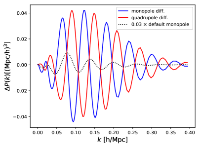
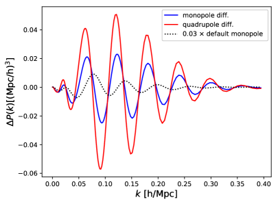
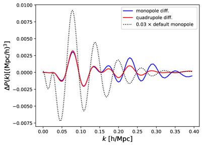
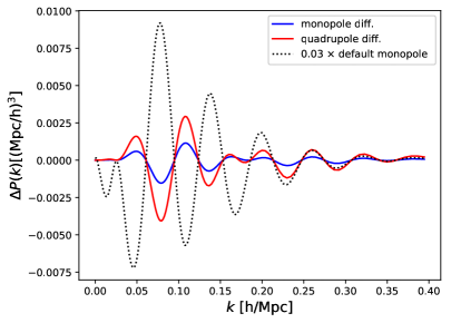
We begin by considering the Fourier space spectra obtained by calculating the multipoles of Eq. (4.6). For different types of ‘wrong reconstruction’, we show the differences between the incorrectly reconstructed monopole and quadrupole power spectra and the correctly reconstructed versions in Fig. 1.

For errors in f𝑓f and b𝑏b, changes of order 1% in the monopole are seen on some scales. Comparing with the default monopole, it can be seen that the incorrect reconstruction spectrum is approximately related to the default reconstruction spectrum by a transfer function that changes the oscillation envelope of the BAO peaks for both monopole and quadrupole, but does not change the peak locations significantly.

A similar conclusion – that the peak positions are not significantly affected by incorrect reconstruction – applies when considering errors in cosmology, i.e. α1subscript𝛼perpendicular-to1\alpha_{\perp}\neq 1 or α1subscript𝛼parallel-to1\alpha_{\parallel}\neq 1; however, it should be noted that in this case, we should not compare the BAO peak scale with the α=1𝛼1\alpha=1 cases, but instead must search for the “extra” shift from incorrect reconstruction by comparing the measured scale with the rescaled correctly reconstructed power spectrum P(𝐤)𝑃superscript𝐤P({\bf k}^{\prime})555The rescaled correctly reconstructed power spectrum is obtained by simply substituting k,ν𝑘𝜈k,\nu by k,μsuperscript𝑘superscript𝜇k^{\prime},\mu^{\prime}, and preserving the normalizing prefactor αα2subscript𝛼parallel-tosuperscriptsubscript𝛼perpendicular-to2\alpha_{\parallel}\alpha_{\perp}^{2} for simpler comparisons..

We now approximately quantify the BAO monopole scale shift in Fourier space; rather than perform a fit for the BAO scale for a certain experimental configuration, we simply use the average of the first peak and trough locations as a rough estimate for the BAO scale (noting that higher peaks give consistent results). For the given errors in αsubscript𝛼perpendicular-to\alpha_{\perp}, αsubscript𝛼parallel-to\alpha_{\parallel}, b𝑏b, f𝑓f we find monopole peak position shifts of order 3×10⁴similar-toabsent3superscript104\sim 3\times 10^{-4} or less compared to the rescaled correctly reconstructed spectrum666An explanation for the non-zero (but still negligible) shifts found for α1𝛼1\alpha\neq 1 could be that the smooth functions multiplying the oscillations (such as the damping factors) are modified by incorrect reconstruction in a way that is anisotropic; therefore, the relative contributions of perpendicular and parallel BAO scales to the BAO monopoles and quadrupoles is changed, resulting in a non-zero shift in the peak positions. This – already negligible – effect could be further reduced by fitting different damping scales in the line-of-sight-perpendicular and parallel directions; or perhaps to some extent by fitting a mean damping scale, as is typically done.. This difference is negligible for experiments operating in the foreseeable future, and likely smaller than shifts induced by terms we have neglected.

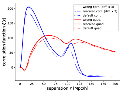
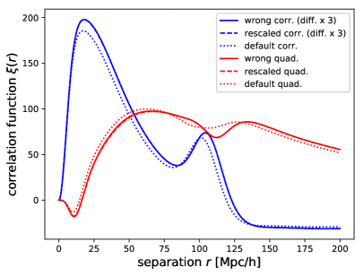
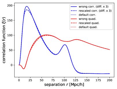
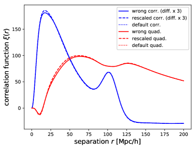
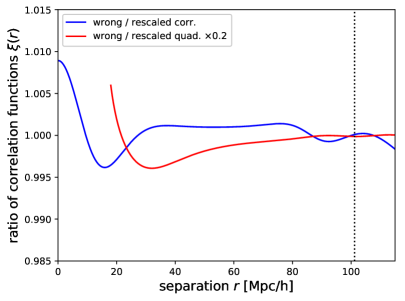
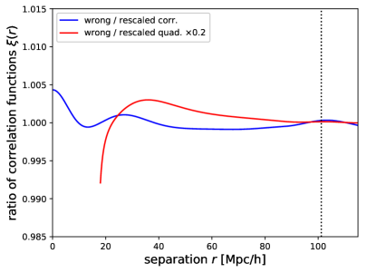
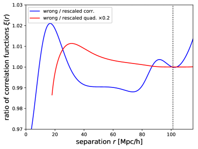
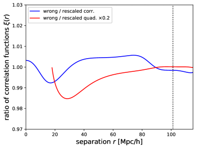
To gain further insight, a configuration space picture is helpful. Appropriately Fourier transforming the power spectra, we obtain the equivalent configuration space correlation functions, which are shown in Fig. 2. We also show the ratio of the correctly and incorrectly reconstructed correlation functions in Fig. 3.

Fig. 3 is particularly illuminating, as it confirms and clarifies our previous discussion. It can be seen from the plots of the correlation function ratios (as well as the correlation functions themselves in Fig. 2) that the BAO peak position is only negligibly affected, with the ratio fairly flat close to the BAO peak scale. Quantifying this, we find that the peak position is only affected at the negligible level of less than 2×10⁴similar-toabsent2superscript104\sim 2\times 10^{-4}, consistent with our Fourier space calculation. However, we see that incorrect reconstruction affects the peak and broadband shapes at the percent level.

Why is the shift in the BAO position so small? To gain more understanding, we Taylor expand the analytical expressions for the reconstructed power spectrum (Eq. 4.6) in small errors 𝚫𝚫\mathbf{\Delta} in parameters such as distances 𝐀=𝟏+𝚫𝐀1𝚫\mathbf{A}=\mathbf{1}+\mathbf{\Delta}. If all first order corrections cancelled, this would provide an explanation for why shifts in the BAO peak scale are so small. However, we find that the linear terms of order 𝚫𝚫\mathbf{\Delta} do not directly cancel when expanding the reconstructed power spectrum; this is consistent with our observation that the broadband is affected substantially by wrong reconstruction (with changes of a few percent, i.e. the same order as the fractional error in distances or other parameters). However, in the limit where the peaks are very narrow – much narrower than the scale over which the damping function varies – we can gain more intuition for the robustness of the position of the BAO peak. One of our key results is that wrong reconstruction only substantially modifies the damping factor D𝐷D in Eq. 4.6, beyond the usual Alcock-Paczynsky rescaling of the biased power spectrum (P(𝐤)P(𝐀𝐤)𝑃𝐤𝑃𝐀𝐤P({\bf k})\rightarrow P(\mathbf{A}{\bf k})). For sharp peaks, simply modifying the slowly-varying damping factor, DD+𝚫D/𝚫𝐷𝐷𝚫𝐷𝚫D\rightarrow D+\mathbf{\Delta}\cdot\partial D/\partial\mathbf{\Delta}, cannot significantly shift the positions of any of the peaks, because the location of an unperturbed maximum or minimum cannot be affected by a sufficiently smooth modulation. While the Alcock-Paczynski rescaling does change the peak positions in the biased power spectrum P𝑃P to leading order in 𝚫𝚫\mathbf{\Delta}, in this case the first order effect is removed by comparing the peak positions to those in the rescaled, correctly reconstructed power spectrum. Since the first order effects in both P𝑃P and D𝐷D are thus removed, the leading order effect is a second order (or higher) one in 𝚫𝚫\mathbf{\Delta} – consistent with the observation of 104similar-toabsentsuperscript104\sim 10^{-4} shifts in the peak positions for a 3%percent33\% error in the distances.

Refer to caption
(a) Wrong αsubscript𝛼perpendicular-to\alpha_{\perp}=1.03
Refer to caption
(b) Wrong αsubscript𝛼parallel-to\alpha_{\parallel}=1.03
Refer to caption
(c) Wrong b=1.1×2𝑏1.12b=1.1\times 2
Refer to caption
(d) Wrong f=1.3×0.55𝑓1.30.55f=1.3\times 0.55
Figure 1: Effect of errors in fiducial cosmology, bias and RSD on the reconstructed power spectra. Shown are the differences between the incorrectly reconstructed power spectra and the correctly reconstructed default ones; the monopole difference is plotted in blue, the quadrupole difference in red. For reference, the default reconstructed power spectrum monopole itself is shown, rescaled by a factor 0.030.030.03, with a black dotted line. (Note that for all power spectra we have isolated the BAO feature by first subtracting a “no-wiggle” power spectrum without oscillations [28] and then dividing by the linear power spectrum amplitude.)
Refer to caption
(a) Wrong αsubscript𝛼perpendicular-to\alpha_{\perp}=1.01
Refer to caption
(b) Wrong αsubscript𝛼parallel-to\alpha_{\parallel}=1.01
Refer to caption
(c) Wrong b=1.1×2𝑏1.12b=1.1\times 2
Refer to caption
(d) Wrong f=1.3×0.55𝑓1.30.55f=1.3\times 0.55
Figure 2: Configuration space picture of wrong reconstruction. Shown are the wrongly reconstructed correlation function (solid line), the rescaled correctly reconstructed correlation function (with 𝐤𝐀𝐤𝐤𝐀𝐤{\bf k}\rightarrow\mathbf{A}\mathbf{k}; dashed line) and the default correctly reconstructed correlation function (dotted line). To show the differences from the default reconstruction more clearly, we add twice the difference with respect to the default reconstruction to the wrong and rescaled curves. The monopole is shown in blue, the quadrupole in red.
Refer to caption
(a) Wrong αsubscript𝛼perpendicular-to\alpha_{\perp}=1.03: ratio
Refer to caption
(b) Wrong αsubscript𝛼parallel-to\alpha_{\parallel}=1.03: ratio
Refer to caption
(c) Wrong b=1.1×2𝑏1.12b=1.1\times 2: ratio
Refer to caption
(d) Wrong f=1.3×0.55𝑓1.30.55f=1.3\times 0.55: ratio
Figure 3: The ratio of the wrongly reconstructed correlation function to the rescaled correctly reconstructed correlation function. As before, blue indicates the monopole, red the quadrupole. The deviation from unity of the quadrupole has been reduced by a factor 555 to fit on the same plot scale (it is also only shown for r>18Mpc/h𝑟18Mpcr>18\mathrm{Mpc}/h, since the zero-crossing of the quadrupole at smaller r𝑟r makes ratios somewhat unstable). It can be seen that no appreciable change in the BAO peak scale results from wrong reconstruction, though the peak shape and quadrupole amplitude can be changed somewhat.

We now turn to the magnitude of the quadrupole. From Fig. 3 (as well as Fig. 1), we note that the size and shape of the quadrupole is affected at the 5%similar-toabsentpercent5\sim 5\% level by even moderate errors in the fiducial cosmology, RSD parameters and biases. Some care must thus be taken when using quadrupole information, especially at small separations r𝑟r, and incorrect reconstruction assumptions should be considered and investigated as a cause of anomalous quadrupole signals.

We also investigate the impact of using a larger smoothing scale Σsm=20Mpc/hsubscriptΣsm20Mpc\Sigma_{\mathrm{sm}}=20~{}\mathrm{Mpc}/h and a smaller scale 10Mpc/h10Mpc10~{}\mathrm{Mpc}/h than that of our default analysis (Σsm=14.1Mpc/hsubscriptΣsm14.1Mpc\Sigma_{\mathrm{sm}}=14.1~{}\mathrm{Mpc}/h). Our previous results for the BAO peak shift still hold in both cases – the shifts we obtain are at the level of 3×1043superscript1043\times 10^{-4} or less and thus negligible. The detailed form of the correlation function, however, is affected at some level by a different scale choice. In particular, the deviations from unity in the correlation function ratio as shown in Fig. 3 increase somewhat (by a factor 1-2 for the monopole, 2-3 for the quadrupole) when we use the smaller 10Mpc/h10Mpc10~{}\mathrm{Mpc}/h smoothing scale; when using the larger smoothing scale, the departures from unity are reduced by a factor 1-2 for the monopole and \approx2 for the quadrupole. Despite this, our results are qualitatively similar in all cases and our conclusions are thus not strongly dependent on the smoothing scale.

A caveat to our analysis is that we have only expanded the non-zero-lag terms in our derivation to leading order in perturbation theory. At higher order, mode-coupling terms are known to enter and lead to shifts in the BAO peak position. However, as mentioned previously, assuming that the errors in the assumed cosmology, bias or RSD parameters are fairly small, any modification of the mode-coupling part will arise from a product of these small errors and the small higher order mode-coupling terms; such terms are thus expected to be negligible.

How do our results compare to previous work based on simulations? In [12], the authors find mean shifts in the BAO scale of order 103absentsuperscript103\leq 10^{-3} when assuming 20% errors on bias and RSD parameters, but given the scatter on their results these shifts do not differ from zero with statistical significance. Errors when assuming a significantly wrong cosmology (Ωm=0.4subscriptΩ𝑚0.4\Omega_{m}=0.4) are larger, but the authors use a linearized template that, the authors note, is expected to fail for large deviations in cosmology. Ref. [30] perform a similar analysis with a wrong fiducial cosmology which differs by 0.5%percent0.50.5\% in the matter density ΩmsubscriptΩ𝑚\Omega_{m}. They find a shift of 9×10⁴absent9superscript104\approx 9\times 10^{-4} for wrong reconstruction. Ref. [31] also investigated BAO reconstruction in presence of errors on the bias parameters, but they focus on the damping and do not report potential shifts.

Thus, while our results are generally in agreement with simulated results, in a few cases the simulations give slightly higher values of the spurious shifts in the BAO scale. One possible explanation for this is that the shape of the BAO peak (or oscillation envelope in Fourier space) is modified in our calculation, which could lead to non-negligible shifts when fitting with an unmodified template. Our work suggests that a straightforward solution to this problem would be to use Eq. (4.6) or a fitting function of a similar form as the expectation value for the power spectrum in constructing a likelihood. We note that the information content might be slightly enhanced by such a choice, as the peak shape or oscillation envelope may contain some information about parameters such as αsubscript𝛼perpendicular-to\alpha_{\perp}. However, it is unclear how much of this information would still be present after marginalizing over all nuisance parameters (such as the damping scale).

As an alternative to modifying the likelihood, one could consider marginalizing the power spectrum measurement not just over an additive broadband component, but also a multiplicative component in Fourier space. Other solutions might include iterating the reconstruction until the cosmology is converged; given that the effects of wrong reconstruction are small, we expect convergence to be rapid (although propagating noise fluctuations through reconstruction could potentially also cause small biases). We defer an exploration of all these ideas to future work.

6 Conclusions

In this paper we have analytically calculated how wrong assumptions about the fiducial cosmology, bias and RSD parameters impact the reconstructed power spectrum. We have derived a full expression for this power spectrum (Eq. 4.6) and have evaluated it for realistic scenarios.

Assuming large but not unrealistic reconstruction errors (3%percent33\% on distances, 10%percent1010\% on bias, 30%percent3030\% on RSD) we find that:

  • The shifts in the BAO monopole peak position(s) in both Fourier and configuration space appear negligible.

  • The shape of the BAO peak or the oscillation envelope in Fourier space can be modified at the percent level. Fitting with a wrong template could potentially lead to small errors in parameter inference; possible solutions include incorporating a wrong-reconstruction template (from Eq. 4.6) in the likelihood, marginalizing over an oscillation envelope shape in a Fourier space analysis, or potentially iterating the reconstruction.

  • The quadrupole can be affected at the 5%percent55\% level by even moderate errors in the assumed cosmology, bias and RSD.

Future research directions include investigating new likelihoods or iterative fitting and examining whether wrong reconstruction impacts BAO constraints on Neffsubscript𝑁effN_{\mathrm{eff}}, the effective number of neutrinos [32, 33].

Acknowledgments

We thank Hee-Jong Seo and Florian Beutler for helpful comments on the draft as well as useful discussions. BDS acknowledges support from an Isaac Newton Trust Early Career Grant as well as an STFC Ernest Rutherford Fellowship. BDS also thanks Lawrence Berkeley Laboratory and the Berkeley Center for Cosmological Physics for hospitality during the completion of this work. MW is supported by the DOE and by NSF.

Appendix A Appendix: Evaluating the incorrectly reconstructed spectra

In this appendix, we will describe in detail the full, general calculation of the incorrectly reconstructed power spectrum outlined in section 4. Following our discussion in section 4, we must evaluate three terms (Pddsubscript𝑃𝑑𝑑P_{dd}, Pdssubscript𝑃𝑑𝑠P_{ds} and Psssubscript𝑃𝑠𝑠P_{ss}). For illustration we will focus on the Pddsubscript𝑃𝑑𝑑P_{dd} term, which is given by

d3qdλ12πdλ22πF(λ1)F(λ2)ei𝐤𝐪exp[i𝐤𝐙𝚿(𝐪2)+i𝐤𝐙𝚿(𝐪1)+iλ2δ(𝐪2)iλ1δ(𝐪1)]superscript𝑑3𝑞𝑑subscript𝜆12𝜋𝑑subscript𝜆22𝜋superscript𝐹subscript𝜆1𝐹subscript𝜆2superscript𝑒𝑖superscript𝐤𝐪delimited-⟨⟩𝑖superscript𝐤subscript𝐙𝚿subscript𝐪2𝑖superscript𝐤subscript𝐙𝚿subscript𝐪1𝑖subscript𝜆2𝛿subscript𝐪2𝑖subscript𝜆1𝛿subscript𝐪1\displaystyle\int d^{3}q\frac{d\lambda_{1}}{2\pi}\frac{d\lambda_{2}}{2\pi}F^{*}(\lambda_{1})F(\lambda_{2})\ e^{-i{\bf k}^{\prime}\cdot{\bf q}}\left\langle\exp\left[-i{\bf k}^{\prime}\cdot\mathbf{Z}_{*}{\bf\Psi}({\bf q}_{2})+i{\bf k}^{\prime}\cdot\mathbf{Z}_{*}{\bf\Psi}({\bf q}_{1})+i\lambda_{2}\delta({\bf q}_{2})-i\lambda_{1}\delta({\bf q}_{1})\right]\right\rangle

where we have defined 𝐙𝐑𝐑~𝐒~𝐙𝐑~𝐑~𝐒\mathbf{Z}\equiv\mathbf{R-\tilde{R}\tilde{S}}. We can evaluate the expectation value with the cumulant theorem as before

exp[i𝐤𝐙𝚿(𝐪2)+i𝐤𝐙𝚿(𝐪1)+iλ2δ(𝐪2)iλ1δ(𝐪1)]delimited-⟨⟩𝑖superscript𝐤subscript𝐙𝚿subscript𝐪2𝑖superscript𝐤subscript𝐙𝚿subscript𝐪1𝑖subscript𝜆2𝛿subscript𝐪2𝑖subscript𝜆1𝛿subscript𝐪1\displaystyle\left\langle\exp\left[-i{\bf k}^{\prime}\cdot\mathbf{Z}_{*}{\bf\Psi}({\bf q}_{2})+i{\bf k}^{\prime}\cdot\mathbf{Z}_{*}{\bf\Psi}({\bf q}_{1})+i\lambda_{2}\delta({\bf q}_{2})-i\lambda_{1}\delta({\bf q}_{1})\right]\right\rangle
=exp[12λ12δ2(𝐪1)+λ22δ2(𝐪2)+2λ1δ(𝐪1)𝐤𝐙𝚿(𝐪2)\displaystyle=\exp\left[-\frac{1}{2}\left\langle\lambda_{1}^{2}\delta^{2}({\bf q}_{1})+\lambda_{2}^{2}\delta^{2}({\bf q}_{2})+2\lambda_{1}\delta({\bf q}_{1}){\bf k}^{\prime}\cdot\mathbf{Z}_{*}{\bf\Psi}({\bf q}_{2})\right.\right.
+2λ2δ(𝐪2)𝐤𝐙𝚿(𝐪1)2λ1λ2δ(𝐪1)δ(𝐪2)]\displaystyle+\left.\left.2\lambda_{2}\delta({\bf q}_{2}){\bf k}^{\prime}\cdot\mathbf{Z}_{*}{\bf\Psi}({\bf q}_{1})-2\lambda_{1}\lambda_{2}\delta({\bf q}_{1})\delta({\bf q}_{2})\right\rangle\right]
×exp[12(𝐤𝐙𝚿(𝐪1)𝐤𝐙𝚿(𝐪2))2]absent12delimited-⟨⟩superscriptsuperscript𝐤subscript𝐙𝚿subscript𝐪1superscript𝐤subscript𝐙𝚿subscript𝐪22\displaystyle\times\exp\left[-\frac{1}{2}\left\langle\left({\bf k}^{\prime}\cdot\mathbf{Z}_{*}{\bf\Psi}({\bf q}_{1})-{\bf k}^{\prime}\cdot\mathbf{Z}_{*}{\bf\Psi}({\bf q}_{2})\right)^{2}\right\rangle\right] (A.1)

We will begin by discussing the non-zero-lag terms. Expanding the exponential, we can perform the q𝑞q and λ𝜆\lambda integrals for all the terms (while keeping the zero-lag parts exponentiated as previously). For example

d3qei𝐤𝐪δ(𝐪1)𝐤𝐙𝚿(𝐪2)superscript𝑑3𝑞superscript𝑒𝑖superscript𝐤𝐪delimited-⟨⟩𝛿subscript𝐪1superscript𝐤subscript𝐙𝚿subscript𝐪2\displaystyle\int d^{3}q\ e^{-i{\bf k}^{\prime}\cdot{\bf q}}\left\langle\delta({\bf q}_{1}){\bf k}^{\prime}\cdot\mathbf{Z}_{*}{\bf\Psi}({\bf q}_{2})\right\rangle
=kjd3qd𝐤1d𝐤2(2π)6ei𝐤𝐪+i𝐤1𝐪1+i𝐤2𝐪2[i𝐙𝐤2k22]jδ(𝐤1)δ(𝐤2)absentsubscriptsuperscript𝑘𝑗superscript𝑑3𝑞𝑑subscript𝐤1𝑑subscript𝐤2superscript2𝜋6superscript𝑒𝑖superscript𝐤𝐪𝑖subscript𝐤1subscript𝐪1𝑖subscript𝐤2subscript𝐪2subscriptdelimited-[]𝑖subscript𝐙𝐤2superscriptsubscript𝑘22𝑗delimited-⟨⟩𝛿subscript𝐤1𝛿subscript𝐤2\displaystyle=k^{\prime}_{j}\int d^{3}q\frac{d{\bf k}_{1}d{\bf k}_{2}}{(2\pi)^{6}}\ e^{-i{\bf k}^{\prime}\cdot{\bf q}+i{\bf k}_{1}\cdot{\bf q}_{1}+i{\bf k}_{2}\cdot{\bf q}_{2}}\left[\frac{i\mathbf{Z}{\bf k}_{2}}{k_{2}^{2}}\right]_{j}\left\langle\delta({\bf k}_{1})\delta({\bf k}_{2})\right\rangle
=kjd3qd𝐤1(2π)3ei𝐤𝐪+i𝐤1𝐪[i𝐙𝐤1k12]jPL(k1)absentsubscriptsuperscript𝑘𝑗superscript𝑑3𝑞𝑑subscript𝐤1superscript2𝜋3superscript𝑒𝑖superscript𝐤𝐪𝑖subscript𝐤1𝐪subscriptdelimited-[]𝑖subscript𝐙𝐤1superscriptsubscript𝑘12𝑗subscript𝑃𝐿subscript𝑘1\displaystyle=k^{\prime}_{j}\int d^{3}q\frac{d{\bf k}_{1}}{(2\pi)^{3}}e^{-i{\bf k}^{\prime}\cdot{\bf q}+i{\bf k}_{1}\cdot{\bf q}}\left[\frac{-i\mathbf{Z}{\bf k}_{1}}{k_{1}^{2}}\right]_{j}P_{L}(k_{1})
=i[𝐤𝐙𝐤]k2PL(k)absent𝑖delimited-[]superscript𝐤superscript𝐙𝐤superscript𝑘2subscript𝑃𝐿superscript𝑘\displaystyle=-i\frac{[{\bf k}^{\prime}\cdot\mathbf{Z}{\bf k}^{\prime}]}{k^{\prime 2}}P_{L}(k^{\prime}) (A.2)

and similarly for the other terms. For the non-zero-lag part of Pddsubscript𝑃𝑑𝑑P_{dd}, in the end we obtain

[𝐤𝐙𝐤]2k4PL(k)+2[𝐤𝐙𝐤]k2FPL(k)+F2PL(k).superscriptdelimited-[]superscript𝐤superscript𝐙𝐤2superscript𝑘4subscript𝑃𝐿superscript𝑘2delimited-[]superscript𝐤superscript𝐙𝐤superscript𝑘2delimited-⟨⟩superscript𝐹subscript𝑃𝐿superscript𝑘superscriptdelimited-⟨⟩superscript𝐹2subscript𝑃𝐿superscript𝑘\displaystyle\frac{[{\bf k}^{\prime}\cdot\mathbf{Z}{\bf k}^{\prime}]^{2}}{k^{\prime 4}}P_{L}(k^{\prime})+2\frac{[{\bf k}^{\prime}\cdot\mathbf{Z}{\bf k}^{\prime}]}{k^{\prime 2}}\langle F^{\prime}\rangle P_{L}(k^{\prime})+\langle F^{\prime}\rangle^{2}P_{L}(k^{\prime}). (A.3)

To simplify factors such as [𝐤𝐙𝐤]=[𝐤(𝐑𝐑~𝐒~)𝐤]delimited-[]superscript𝐤superscript𝐙𝐤delimited-[]superscript𝐤𝐑~𝐑~𝐒superscript𝐤[{\bf k}^{\prime}\cdot\mathbf{Z}{\bf k}^{\prime}]=[{\bf k}^{\prime}\cdot\mathbf{(R-\tilde{R}\tilde{S})}{\bf k}^{\prime}], we note that

𝐤𝐑~𝐀𝟐𝐤k2|𝐀1𝐤|2=(𝐀𝟏𝐤)𝐑~(𝐀𝟏𝐤)k2|𝐀1𝐤|2=(1+f~μ𝐀𝟏𝐤2)k2,{\bf k}^{\prime}\cdot\mathbf{\tilde{R}~{}A^{-2}}{\bf k}^{\prime}\frac{k^{{}^{\prime}2}}{|\mathbf{A}^{-1}{\bf k}^{\prime}|^{2}}=(\mathbf{A^{-1}}{\bf k}^{\prime})\cdot\mathbf{\tilde{R}}(\mathbf{A^{-1}}{\bf k}^{\prime})\frac{k^{{}^{\prime}2}}{|\mathbf{A}^{-1}{\bf k}^{\prime}|^{2}}=\left(1+\tilde{f}\mu_{\mathbf{A^{-1}}{\bf k}}^{2}\right)k^{{}^{\prime}2}, (A.4)

where we have made use of the fact that ν2μ𝐀𝟏𝐤2=[(𝐀𝟏𝐤)𝐳^/|A1𝐤|]2superscript𝜈2superscriptsubscript𝜇superscript𝐀1𝐤2superscriptdelimited-[]superscript𝐀1𝐤^𝐳superscript𝐴1𝐤2\nu^{2}\equiv\mu_{\mathbf{A^{-1}}{\bf k}}^{2}=\left[(\mathbf{A^{-1}}{\bf k})\cdot\mathbf{\hat{z}}/|A^{-1}{\bf k}|\right]^{2} in the second equality. Since [𝐤𝐑𝐤]=(1+fμ2)k2[{\bf k}^{\prime}\cdot\mathbf{R}{\bf k}^{\prime}]=(1+f\mu^{\prime 2})k^{{}^{\prime}2}, it follows that

[𝐤𝐙𝐤]k2=[(1+fμ2)(1+f~ν2)[b+fμ2b~+f~ν2]S(𝐀𝟏𝐤)].delimited-[]superscript𝐤superscript𝐙𝐤superscript𝑘2delimited-[]1𝑓superscript𝜇21~𝑓superscript𝜈2delimited-[]𝑏𝑓superscript𝜇2~𝑏~𝑓superscript𝜈2𝑆superscript𝐀1superscript𝐤\frac{[{\bf k}^{\prime}\cdot\mathbf{Z}{\bf k}^{\prime}]}{k^{\prime 2}}=\left[(1+f\mu^{\prime 2})-(1+\tilde{f}\nu^{2})\left[\frac{b+f\mu^{\prime 2}}{{\tilde{b}+\tilde{f}\nu^{2}}}\right]S(\mathbf{A^{-1}}{\bf k}^{\prime})\right]. (A.5)

Using F=b1delimited-⟨⟩superscript𝐹𝑏1\langle F^{\prime}\rangle=b-1 we can now evaluate the non-zero-lag part of the Pddsubscript𝑃𝑑𝑑P_{dd} term

[𝐤𝐙𝐤]2k4PL(k)+2[𝐤𝐙𝐤]k2FPL(k)+F2PL(k)superscriptdelimited-[]superscript𝐤superscript𝐙𝐤2superscript𝑘4subscript𝑃𝐿superscript𝑘2delimited-[]superscript𝐤superscript𝐙𝐤superscript𝑘2delimited-⟨⟩superscript𝐹subscript𝑃𝐿superscript𝑘superscriptdelimited-⟨⟩superscript𝐹2subscript𝑃𝐿superscript𝑘\displaystyle\hphantom{=}\frac{[{\bf k}^{\prime}\cdot\mathbf{Z}{\bf k}^{\prime}]^{2}}{k^{\prime 4}}P_{L}(k^{\prime})+2\frac{[{\bf k}^{\prime}\cdot\mathbf{Z}{\bf k}^{\prime}]}{k^{\prime 2}}\langle F^{\prime}\rangle P_{L}(k^{\prime})+\langle F^{\prime}\rangle^{2}P_{L}(k^{\prime})
=([b1]+[𝐤𝐙𝐤]k2)2PL(k)absentsuperscriptdelimited-[]𝑏1delimited-[]superscript𝐤superscript𝐙𝐤superscript𝑘22subscript𝑃𝐿superscript𝑘\displaystyle=\left(\left[b-1\right]+\frac{[{\bf k}^{\prime}\cdot\mathbf{Z}{\bf k}^{\prime}]}{k^{\prime 2}}\right)^{2}P_{L}(k^{\prime})
=[b+fμ2]2[1[1+f~ν2b~+f~ν2]S(𝐀1𝐤)]2PL(k).absentsuperscriptdelimited-[]𝑏𝑓superscript𝜇22superscriptdelimited-[]1delimited-[]1~𝑓superscript𝜈2~𝑏~𝑓superscript𝜈2𝑆superscript𝐀1superscript𝐤2subscript𝑃𝐿superscript𝑘\displaystyle=[b+f\mu^{\prime 2}]^{2}\left[1-\left[\frac{1+\tilde{f}\nu^{2}}{\tilde{b}+\tilde{f}\nu^{2}}\right]S(\mathbf{A}^{-1}{\bf k}^{\prime})\right]^{2}P_{L}(k^{\prime}). (A.6)

Performing a similar analysis for the Psssubscript𝑃𝑠𝑠P_{ss} term, the non-zero-lag piece is

[𝐤𝐑~𝐒~𝐤]2k4PL(k)=[b+fμ2]2[1+f~ν2b~+f~ν2S(𝐀1𝐤)]2PL(k).superscriptdelimited-[]superscript𝐤~𝐑~𝐒superscript𝐤2superscript𝑘4subscript𝑃𝐿superscript𝑘superscriptdelimited-[]𝑏𝑓superscript𝜇22superscriptdelimited-[]1~𝑓superscript𝜈2~𝑏~𝑓superscript𝜈2𝑆superscript𝐀1superscript𝐤2subscript𝑃𝐿superscript𝑘\displaystyle\frac{\left[{\bf k}^{\prime}\cdot\mathbf{\tilde{R}~{}\tilde{S}}{\bf k}^{\prime}\right]^{2}}{k^{\prime 4}}P_{L}(k^{\prime})=[b+f\mu^{\prime 2}]^{2}\left[\frac{1+\tilde{f}\nu^{2}}{\tilde{b}+\tilde{f}\nu^{2}}S(\mathbf{A}^{-1}{\bf k}^{\prime})\right]^{2}P_{L}(k^{\prime}).

For Pdssubscript𝑃𝑑𝑠P_{ds}, the relevant piece is

[𝐤𝐙𝐤][𝐤𝐑~𝐒~𝐤]k4PL(k)+F[𝐤𝐑~𝐒~𝐤]k2PL(k)delimited-[]superscript𝐤superscript𝐙𝐤delimited-[]superscript𝐤~𝐑~𝐒superscript𝐤superscript𝑘4subscript𝑃𝐿superscript𝑘delimited-⟨⟩superscript𝐹delimited-[]superscript𝐤~𝐑~𝐒superscript𝐤superscript𝑘2subscript𝑃𝐿superscript𝑘\displaystyle\frac{[{\bf k}^{\prime}\cdot\mathbf{Z}{\bf k}^{\prime}]\left[{\bf k}^{\prime}\cdot\mathbf{\tilde{R}\tilde{S}}{\bf k}^{\prime}\right]}{k^{4}}P_{L}(k^{\prime})+\langle F^{\prime}\rangle\frac{\left[{\bf k}^{\prime}\cdot\mathbf{\tilde{R}\tilde{S}}{\bf k}^{\prime}\right]}{k^{\prime 2}}P_{L}(k^{\prime}) (A.7)
=\displaystyle= ([b1]+[𝐤𝐙𝐤]k2)[𝐤𝐑~𝐒~𝐤]k2PL(k)delimited-[]𝑏1delimited-[]superscript𝐤superscript𝐙𝐤superscript𝑘2delimited-[]superscript𝐤~𝐑~𝐒superscript𝐤superscript𝑘2subscript𝑃𝐿superscript𝑘\displaystyle\left(\left[b-1\right]+\frac{[{\bf k}^{\prime}\cdot\mathbf{Z}{\bf k}^{\prime}]}{k^{\prime 2}}\right)\frac{\left[{\bf k}^{\prime}\cdot\mathbf{\tilde{R}\tilde{S}}{\bf k}^{\prime}\right]}{k^{\prime 2}}P_{L}(k^{\prime})
=\displaystyle= [b+fμ2]2[11+f~ν2b~+f~ν2S(𝐀1𝐤)][1+f~ν2b~+f~ν2S(𝐀1𝐤)]PL(k).superscriptdelimited-[]𝑏𝑓superscript𝜇22delimited-[]11~𝑓superscript𝜈2~𝑏~𝑓superscript𝜈2𝑆superscript𝐀1superscript𝐤delimited-[]1~𝑓superscript𝜈2~𝑏~𝑓superscript𝜈2𝑆superscript𝐀1superscript𝐤subscript𝑃𝐿superscript𝑘\displaystyle[b+f\mu^{2}]^{2}\left[1-\frac{1+\tilde{f}\nu^{2}}{\tilde{b}+\tilde{f}\nu^{2}}S(\mathbf{A}^{-1}{\bf k}^{\prime})\right]\left[\frac{1+\tilde{f}\nu^{2}}{\tilde{b}+\tilde{f}\nu^{2}}S(\mathbf{A}^{-1}{\bf k}^{\prime})\right]P_{L}(k^{\prime}).

Finally, we consider the zero-lag piece of all three terms. For this calculation, it will be convenient to define a new function g𝑔g as follows:

𝐒(𝐤)=𝐀2[k2|𝐀1𝐤|2b+fμ2b~+f~ν2]S(𝐀1𝐤)𝐀2g(𝐤)S(𝐀1𝐤),\displaystyle\mathbf{S}({\bf k}^{\prime})=\mathbf{A}^{-2}\left[\frac{k^{{}^{\prime}2}}{|\mathbf{A}^{-1}{\bf k}^{\prime}|^{2}}\frac{b+f\mu^{\prime 2}}{{\tilde{b}+\tilde{f}\nu^{2}}}\right]S(\mathbf{A}^{-1}{\bf k}^{\prime})\equiv\mathbf{A}^{-2}g({\bf k}^{\prime})S(\mathbf{A}^{-1}{\bf k}^{\prime}), (A.8)

where g(𝐤)𝑔superscript𝐤g({\bf k}^{\prime}) is the factor in square brackets. For the zero-lag piece of the Psssubscript𝑃𝑠𝑠P_{ss} term, we obtain

=\displaystyle= exp[iki2d𝐤1(2π)3[𝐑~𝐀𝟐𝐤1]i2g2(𝐤1)S2(𝐀𝟏𝐤1)PL(k1)k14]\displaystyle\exp\left[-\sum_{i}k_{i}^{{}^{\prime}2}\int\frac{d{\bf k}_{1}}{(2\pi)^{3}}\left[\mathbf{\tilde{R}A^{-2}}{\bf k}_{1}\right]_{i}^{2}g^{2}({\bf k}_{1})S^{2}(\mathbf{A^{-1}}{\bf k}_{1})\frac{P_{L}(k_{1})}{k_{1}^{4}}\right] (A.9)
=\displaystyle= exp[k2d𝐤1(2π)3(1μ12)k12g2(𝐤1)S2(𝐀𝟏𝐤1)PL(k1)2k14α4\displaystyle\exp\bigg{[}-k_{\bot}^{{}^{\prime}2}\int\frac{d{\bf k}_{1}}{(2\pi)^{3}}(1-\mu_{1}^{2})k_{1}^{2}g^{2}({\bf k}_{1})S^{2}(\mathbf{A^{-1}}{\bf k}_{1})\frac{P_{L}(k_{1})}{2k_{1}^{4}\alpha_{\bot}^{4}}
\displaystyle- k2(1+f~)2d𝐤1(2π)3μ12k12g2(𝐤1)S2(𝐀𝟏𝐤1)PL(k1)k14α4]\displaystyle k_{\parallel}^{{}^{\prime}2}(1+\tilde{f})^{2}\int\frac{d{\bf k}_{1}}{(2\pi)^{3}}\mu_{1}^{2}k_{1}^{2}g^{2}({\bf k}_{1})S^{2}(\mathbf{A^{-1}}{\bf k}_{1})\frac{P_{L}(k_{1})}{k_{1}^{4}\alpha_{\parallel}^{4}}\bigg{]}
exp[12k2Σss,2f~,b~,𝐀12k2(1+f~)2Σss,2f~,b~,𝐀],\displaystyle\equiv\exp\left[-\frac{1}{2}k_{\bot}^{{}^{\prime}2}\Sigma^{2~{}\tilde{f},\tilde{b},\mathbf{A}}_{ss,\bot}-\frac{1}{2}k_{\parallel}^{{}^{\prime}2}(1+\tilde{f})^{2}\Sigma^{2~{}\tilde{f},\tilde{b},\mathbf{A}}_{ss,\parallel}\right],

where the last line defines new damping functions from the two terms in the previous exponent. Similarly, for Pddsubscript𝑃𝑑𝑑P_{dd} we obtain:

exp[k2d𝐤1(2π)3(1μ2)k12(1g(𝐤1)S(𝐀𝟏𝐤1)α2)2PL(k1)2k14\displaystyle\exp\bigg{[}-k_{\bot}^{{}^{\prime}2}\int\frac{d{\bf k}_{1}}{(2\pi)^{3}}(1-\mu^{2})k_{1}^{2}(1-\frac{g({\bf k}_{1})S(\mathbf{A^{-1}}{\bf k}_{1})}{\alpha_{\bot}^{2}})^{2}\frac{P_{L}(k_{1})}{2k_{1}^{4}} (A.10)
\displaystyle- k2(1+f)2d𝐤1(2π)3μ2k12(11+f~(1+f)α2g(𝐤1)S(𝐀𝟏𝐤1))2PL(k1)k14]\displaystyle k_{\parallel}^{{}^{\prime}2}(1+f)^{2}\int\frac{d{\bf k}_{1}}{(2\pi)^{3}}\mu^{2}k_{1}^{2}(1-\frac{1+\tilde{f}}{(1+f)\alpha_{\parallel}^{2}}g({\bf k}_{1})S(\mathbf{A^{-1}}{\bf k}_{1}))^{2}\frac{P_{L}(k_{1})}{k_{1}^{4}}\bigg{]}
\displaystyle\equiv exp[12k2Σdd,2f~,b~,𝐀12k2(1+f)2Σdd,2f~,b~,𝐀]\displaystyle\exp\left[-\frac{1}{2}k_{\bot}^{{}^{\prime}2}\Sigma^{2~{}\tilde{f},\tilde{b},\mathbf{A}}_{dd,\bot}-\frac{1}{2}k_{\parallel}^{{}^{\prime}2}(1+f)^{2}\Sigma^{2~{}\tilde{f},\tilde{b},\mathbf{A}}_{dd,\parallel}\right]

The exponent of the Pdssubscript𝑃𝑑𝑠P_{ds} term is given by the average of the Psssubscript𝑃𝑠𝑠P_{ss} and Pddsubscript𝑃𝑑𝑑P_{dd} term exponents as previously.

Assembling these results gives our most general equation for the reconstructed power spectrum with errors in angle, distance, bias, and RSD. The final expression is:

Precf(𝐤)superscriptsubscript𝑃rec𝑓𝐤\displaystyle P_{\mathrm{rec}}^{f}({\bf k}) =α2α[b+fμ2]2PL(k){[1+f~ν2b~+f~ν2S(k)]2𝒟ss\displaystyle=\alpha_{\bot}^{2}\alpha_{\parallel}\left[b+f\mu^{{}^{\prime}2}\right]^{2}P_{L}(k^{\prime})\left\{\left[\frac{1+\tilde{f}\nu^{2}}{\tilde{b}+\tilde{f}\nu^{2}}S(k)\right]^{2}\mathcal{D}_{ss}\right.
+[11+f~ν2b~+f~ν2S(k)]2𝒟dd+2[11+f~ν2b~+f~ν2S(k)][1+f~ν2b~+f~ν2S(k)]𝒟ds},\displaystyle+\left.\left[1-\frac{1+\tilde{f}\nu^{2}}{\tilde{b}+\tilde{f}\nu^{2}}S(k)\right]^{2}\mathcal{D}_{dd}+2\left[1-\frac{1+\tilde{f}\nu^{2}}{\tilde{b}+\tilde{f}\nu^{2}}S(k)\right]\left[\frac{1+\tilde{f}\nu^{2}}{\tilde{b}+\tilde{f}\nu^{2}}S(k)\right]\mathcal{D}_{ds}\right\}, (A.11)

where

2ln𝒟ss2subscript𝒟𝑠𝑠\displaystyle-2\ln\mathcal{D}_{ss} =k2Σss,2f~,b~,𝐀+k2(1+f~)2Σss,2f~,b~,𝐀\displaystyle=k_{\bot}^{{}^{\prime}2}\Sigma^{{2~{}\tilde{f},\tilde{b},\mathbf{A}}}_{ss,\bot}+k_{\parallel}^{{}^{\prime}2}(1+\tilde{f})^{2}\Sigma^{{2~{}\tilde{f},\tilde{b},\mathbf{A}}}_{ss,\parallel} (A.12)
2ln𝒟dd2subscript𝒟𝑑𝑑\displaystyle-2\ln\mathcal{D}_{dd} =k2Σdd,2f~,b~,𝐀+k2(1+f)2Σdd,2f~,b~,𝐀\displaystyle=k_{\bot}^{{}^{\prime}2}\Sigma^{{2~{}\tilde{f},\tilde{b},\mathbf{A}}}_{dd,\bot}+k_{\parallel}^{{}^{\prime}2}(1+f)^{2}\Sigma^{{2~{}\tilde{f},\tilde{b},\mathbf{A}}}_{dd,\parallel} (A.13)
2ln𝒟ds2subscript𝒟𝑑𝑠\displaystyle-2\ln\mathcal{D}_{ds} =12[2ln𝒟dd2ln𝒟ss],absent12delimited-[]2subscript𝒟𝑑𝑑2subscript𝒟𝑠𝑠\displaystyle=\frac{1}{2}\left[-2\ln\mathcal{D}_{dd}-2\ln\mathcal{D}_{ss}\right], (A.14)

the damping coefficients ΣΣ\Sigma are defined in Eqs. (A.9-A.10) above, and we remind the reader that 𝐤=𝐀𝟏𝐤𝐤superscript𝐀1superscript𝐤{\bf k}=\mathbf{A^{-1}k^{\prime}} and ν=𝐤^𝐳^𝜈^𝐤^𝐳\nu=\hat{{\bf k}}\cdot\hat{\mathbf{z}}.

References

  • [1] S. Alam, M. Ata, S. Bailey, F. Beutler, D. Bizyaev, J. A. Blazek, A. S. Bolton, J. R. Brownstein, A. Burden, C.-H. Chuang, J. Comparat, A. J. Cuesta, K. S. Dawson, D. J. Eisenstein, S. Escoffier, H. Gil-Marín, J. N. Grieb, N. Hand, S. Ho, K. Kinemuchi, D. Kirkby, F. Kitaura, E. Malanushenko, V. Malanushenko, C. Maraston, C. K. McBride, R. C. Nichol, M. D. Olmstead, D. Oravetz, N. Padmanabhan, N. Palanque-Delabrouille, K. Pan, M. Pellejero-Ibanez, W. J. Percival, P. Petitjean, F. Prada, A. M. Price-Whelan, B. A. Reid, S. A. Rodríguez-Torres, N. A. Roe, A. J. Ross, N. P. Ross, G. Rossi, J. A. Rubiño-Martín, A. G. Sánchez, S. Saito, S. Salazar-Albornoz, L. Samushia, S. Satpathy, C. G. Scóccola, D. J. Schlegel, D. P. Schneider, H.-J. Seo, A. Simmons, A. Slosar, M. A. Strauss, M. E. C. Swanson, D. Thomas, J. L. Tinker, R. Tojeiro, M. Vargas Magaña, J. A. Vazquez, L. Verde, D. A. Wake, Y. Wang, D. H. Weinberg, M. White, W. M. Wood-Vasey, C. Yèche, I. Zehavi, Z. Zhai, and G.-B. Zhao, The clustering of galaxies in the completed SDSS-III Baryon Oscillation Spectroscopic Survey: cosmological analysis of the DR12 galaxy sample, ArXiv e-prints (July, 2016) [arXiv:1607.03155].
  • [2] D. H. Weinberg, M. J. Mortonson, D. J. Eisenstein, C. Hirata, A. G. Riess, and E. Rozo, Observational probes of cosmic acceleration, Physics Reports 530 (Sept., 2013) 87–255, [arXiv:1201.2434].
  • [3] Particle Data Group Collaboration, K. Olive et al., Review of Particle Physics, Chin.Phys. C38 (2014) 090001.
  • [4] D. J. Eisenstein, H.-J. Seo, E. Sirko, and D. N. Spergel, Improving Cosmological Distance Measurements by Reconstruction of the Baryon Acoustic Peak, ApJ 664 (Aug., 2007) 675–679, [astro-ph/0604362].
  • [5] N. Padmanabhan, M. White, and J. D. Cohn, Reconstructing baryon oscillations: A Lagrangian theory perspective, PRD 79 (Mar., 2009) 063523, [arXiv:0812.2905].
  • [6] Y. Noh, M. White, and N. Padmanabhan, Reconstructing baryon oscillations, PRD 80 (Dec., 2009) 123501, [arXiv:0909.1802].
  • [7] H.-J. Seo, J. Eckel, D. J. Eisenstein, K. Mehta, M. Metchnik, N. Padmanabhan, P. Pinto, R. Takahashi, M. White, and X. Xu, High-precision Predictions for the Acoustic Scale in the Nonlinear Regime, ApJ 720 (Sept., 2010) 1650–1667, [arXiv:0910.5005].
  • [8] N. Padmanabhan, X. Xu, D. J. Eisenstein, R. Scalzo, A. J. Cuesta, K. T. Mehta, and E. Kazin, A 2 per cent distance to z = 0.35 by reconstructing baryon acoustic oscillations - I. Methods and application to the Sloan Digital Sky Survey, Mon. Not. R. Astron. Soc 427 (Dec., 2012) 2132–2145, [arXiv:1202.0090].
  • [9] S. Tassev and M. Zaldarriaga, Towards an optimal reconstruction of baryon oscillations, JCAP 10 (Oct., 2012) 006, [arXiv:1203.6066].
  • [10] N. McCullagh and A. S. Szalay, Nonlinear Behavior of Baryon Acoustic Oscillations from the Zel’dovich Approximation Using a Non-Fourier Perturbation Approach, ApJ 752 (June, 2012) 21, [arXiv:1202.1306].
  • [11] B. D. Sherwin and M. Zaldarriaga, Shift of the baryon acoustic oscillation scale: A simple physical picture, PRD 85 (May, 2012) 103523, [arXiv:1202.3998].
  • [12] X. Xu, A. J. Cuesta, N. Padmanabhan, D. J. Eisenstein, and C. K. McBride, Measuring DA and H at z=0.35 from the SDSS DR7 LRGs using baryon acoustic oscillations, Mon. Not. R. Astron. Soc 431 (May, 2013) 2834–2860, [arXiv:1206.6732].
  • [13] M. Schmittfull, Y. Feng, F. Beutler, B. Sherwin, and M. Y. Chu, Eulerian BAO reconstructions and N -point statistics, PRD 92 (Dec., 2015) 123522, [arXiv:1508.06972].
  • [14] A. Burden, W. J. Percival, and C. Howlett, Reconstruction in Fourier space, Mon. Not. R. Astron. Soc 453 (Oct., 2015) 456–468, [arXiv:1504.02591].
  • [15] I. Achitouv and C. Blake, Improving reconstruction of the baryon acoustic peak: The effect of local environment, PRD 92 (Oct., 2015) 083523, [arXiv:1507.03584].
  • [16] M. White, Reconstruction within the Zeldovich approximation, Mon. Not. R. Astron. Soc 450 (July, 2015) 3822–3828, [arXiv:1504.03677].
  • [17] J. D. Cohn, M. White, T.-C. Chang, G. Holder, N. Padmanabhan, and O. Doré, Combining galaxy and 21-cm surveys, Mon. Not. R. Astron. Soc 457 (Apr., 2016) 2068–2077, [arXiv:1511.07377].
  • [18] H.-J. Seo, F. Beutler, A. J. Ross, and S. Saito, Modeling the reconstructed BAO in Fourier space, Mon. Not. R. Astron. Soc 460 (Aug., 2016) 2453–2471, [arXiv:1511.00663].
  • [19] M. Vargas-Magaña, S. Ho, A. J. Cuesta, R. O’Connell, A. J. Ross, D. J. Eisenstein, W. J. Percival, J. N. Grieb, A. G. Sánchez, J. L. Tinker, R. Tojeiro, F. Beutler, C.-H. Chuang, F.-S. Kitaura, F. Prada, S. A. Rodríguez-Torres, G. Rossi, H.-J. Seo, J. R. Brownstein, M. Olmstead, and D. Thomas, The clustering of galaxies in the completed SDSS-III Baryon Oscillation Spectroscopic Survey: theoretical systematics and Baryon Acoustic Oscillations in the galaxy correlation function, ArXiv e-prints (Oct., 2016) [arXiv:1610.03506].
  • [20] C. Hikage, K. Koyama, and A. Heavens, Perturbation Theory for BAO reconstructed fields: one-loop results in real-space matter density field, ArXiv e-prints (Mar., 2017) [arXiv:1703.07878].
  • [21] Y. B. Zel’dovich, Gravitational instability: An approximate theory for large density perturbations., A&A 5 (Mar., 1970) 84–89.
  • [22] T. Matsubara, Resumming cosmological perturbations via the Lagrangian picture: One-loop results in real space and in redshift space, PRD 77 (Mar., 2008) 063530, [arXiv:0711.2521].
  • [23] T. Matsubara, Nonlinear perturbation theory with halo bias and redshift-space distortions via the Lagrangian picture, PRD 78 (Oct., 2008) 083519, [arXiv:0807.1733].
  • [24] S. Tassev and M. Zaldarriaga, The mildly non-linear regime of structure formation, JCAP 4 (Apr., 2012) 013, [arXiv:1109.4939].
  • [25] J. Carlson, B. Reid, and M. White, Convolution Lagrangian perturbation theory for biased tracers, Mon. Not. R. Astron. Soc 429 (Feb., 2013) 1674–1685, [arXiv:1209.0780].
  • [26] S. Bharadwaj, The Evolution of Correlation Functions in the Zeldovich Approximation and Its Implications for the Validity of Perturbation Theory, ApJ 472 (Nov., 1996) 1–+, [astro-ph/9].
  • [27] E. Castorina and M. White, The Zeldovich approximation and wide-angle redshift-space distortions, Mon. Not. R. Astron. Soc 479 (Sept., 2018) 741–752, [arXiv:1803.08185].
  • [28] D. J. Eisenstein and W. Hu, Power Spectra for Cold Dark Matter and Its Variants, ApJ 511 (Jan., 1999) 5–15, [astro-ph/9710252].
  • [29] Planck Collaboration, P. A. R. Ade, N. Aghanim, M. Arnaud, M. Ashdown, J. Aumont, C. Baccigalupi, A. J. Banday, R. B. Barreiro, J. G. Bartlett, and et al., Planck 2015 results. XIII. Cosmological parameters, A&A 594 (Sept., 2016) A13, [arXiv:1502.01589].
  • [30] M. Vargas-Magaña, S. Ho, A. J. Cuesta, R. O’Connell, A. J. Ross, D. J. Eisenstein, W. J. Percival, J. N. Grieb, A. G. Sánchez, J. L. Tinker, R. Tojeiro, F. Beutler, C.-H. Chuang, F.-S. Kitaura, F. Prada, S. A. Rodríguez-Torres, G. Rossi, H.-J. Seo, J. R. Brownstein, M. Olmstead, and D. Thomas, The clustering of galaxies in the completed SDSS-III Baryon Oscillation Spectroscopic Survey: theoretical systematics and Baryon Acoustic Oscillations in the galaxy correlation function, Mon. Not. R. Astron. Soc 477 (June, 2018) 1153–1188.
  • [31] K. T. Mehta, H.-J. Seo, J. Eckel, D. J. Eisenstein, M. Metchnik, P. Pinto, and X. Xu, Galaxy Bias and Its Effects on the Baryon Acoustic Oscillation Measurements, ApJ 734 (June, 2011) 94, [arXiv:1104.1178].
  • [32] D. Baumann, D. Green, and B. Wallisch, Searching for Light Relics with Large-Scale Structure, ArXiv e-prints (Dec., 2017) [arXiv:1712.08067].
  • [33] D. Baumann, F. Beutler, R. Flauger, D. Green, M. Vargas-Magaña, A. Slosar, B. Wallisch, and C. Yèche, First Measurement of Neutrinos in the BAO Spectrum, ArXiv e-prints (Mar., 2018) [arXiv:1803.10741].