On the Relation Between Mobile Encounters and Web Traffic Patterns: A Data-driven Study

Abstract.

Mobility and network traffic have been traditionally studied separately. Their interaction is vital for generations of future mobile services and effective caching, but has not been studied in depth with real-world big data. In this paper, we characterize mobility encounters and study the correlation between encounters and web traffic profiles using large-scale datasets (30TB in size) of WiFi and NetFlow traces. The analysis quantifies these correlations for the first time, across spatio-temporal dimensions, for device types grouped into on-the-go Flutes and sit-to-use Cellos. The results consistently show a clear relation between mobility encounters and traffic across different buildings over multiple days, with encountered pairs showing higher traffic similarity than non-encountered pairs, and long encounters being associated with the highest similarity. We also investigate the feasibility of learning encounters through web traffic profiles, with implications for dissemination protocols, and contact tracing. This provides a compelling case to integrate both mobility and web traffic dimensions in future models, not only at an individual level, but also at pairwise and collective levels. We have released samples of code and data used in this study on GitHub, to support reproducibility and encourage further research (https://github.com/BabakAp/encounter-traffic).

1. Introduction & Related work

The effect of mobility and network traffic on wireless networks has been clearly established in the literature (e.g. (Important, )). Several efforts studied models of mobility and network traffic, albeit mostly separately and in isolation. There is a vast body of research focused on mobility or traffic independently, which we cannot possibly exhaustively cover. We refer the reader to (treuniet:csur14, ; hess:csur16, ) for surveys of mobility modeling and analysis. Some of the most advanced studies on mobility (Cobra, ) have identified individual (TVC, ), pairwise (encounter), and collective (group) dimensions for mobility modeling. That study, however, did not consider traffic. We hope to bridge that gap by analyzing the interplay of mobility and traffic at the pairwise level.

We argue that the relation between mobility and traffic needs further in-depth analysis, as it will likely be the center of many future mobile services. In this paper, we focus on the pairwise (encounter) dimension of mobility and study its interplay with the traffic patterns of mobile users. Aside from this study’s importance to realistic modeling, simulation and performance evaluation of next-generation networks, it is quite relevant to encounter-based services, e.g., content sharing, opportunistic networking, mobile social networks, and encounter-based trust and homophily ((manweiler2009smile, ; dong2014inferring, )), to name a few.

Encounters between mobile nodes have been studied in previous research (e.g., in (enNodal, ; enMetric, )) to characterize opportunities of inter-user encounters. Others (e.g., (EncCollection1, ; EncCollection2, )), mainly collect encounter traces using mobile devices to analyze, model and understand communication opportunities in different settings. None of these studies, however, analyze traffic nor the correlation between encounters and real-world traffic patterns. In this study, we focus on the interplay between traffic and encounters, while considering the score (e.g., duration, frequency) of the encounter events. We use extensive data-driven analyses to quantify the correlations between network traffic and encounter scores.

Several studies analyzed wireless traffic flows (FlowStudy, ), and mobile web-visitation patterns (Saeed, ). These studies, however, did not investigate the relation with mobility and node encounters.

In addition, many research studies on mobility encounters or traffic patterns did not consider device type. Devices’ form factor affects mode of usage, leading to varied traffic profiles ((afanasyev2008analysis, ; maier2010first, ; Falaki2010, ; chen2012network, ; Kumar2013, ; gember2011comparative, ; papapanagiotou2012smartphones, )). But these studies do not study the interplay of traffic with mobility and encounters. These devices are also used during different modes of transportation. Smartphones and e-readers, which we refer to as Flutes, are devices used ’on-the-go’. On the other hand, laptops are ’sit-to-use’ devices and are referred to as Cellos in this study. In our earlier work (Alipour2018, ), we contrast various mobility and traffic features of Flutes and Cellos, including radius of gyration, location visitation preferences, and flow-level statistics. But that study only investigated mobility and traffic features across the individual dimension. While we investigate the pairwise dimension here, focusing on encounter-traffic interplay while considering the device types.

We use extensive traces from our collected datasets (with $76$B records, and $\approx$30TB in size) covering over 78K devices, in 140 buildings on a university campus. The data includes information about WiFi associations, as well as DHCP and NetFlow traces, covering the dimensions of mobility and network traffic. The data is sanitized and categorized based on buildings, days, device types (Flutes, Cellos), and encounter duration, then the analysis is done across all these dimensions.

The main question addressed in this study is ‘How do device encounters affect network traffic patterns, across time, space, device type and encounter duration?’ For that purpose, we: i- analyze mobility encounters patterns, ii- define web traffic profiles for users, and iii- look at their interplay. Although this question has not been directly studied in-depth before, our findings are quite surprising, showing that for the majority of buildings a consistent correlation exists between traffic profiles and encountered (vs. non-encountered) pairs of users. We also found the correlation to be the strongest for Cello-Cello encounters on weekends. Further, we find that such relation strengthens for long encounters, while short encounters are not significantly different from non-encountered pairs. Finally, we utilized a deep learning model to learn encounters of user pairs in a day and building based on their traffic profiles alone. The model achieved a high accuracy (90%+) in many settings, with major implications for encounter-based services, rumor anatomy analysis, and infection tracing.

These results can potentially impact a variety of applications, including those utilizing prediction of traffic load/demand using encounters, and vice versa. In addition, mobility modeling and protocol evaluation could benefit from deep integration of (and the interplay between) encounters and traffic. We hope for this paper to be the first in a series of studies on mobility and traffic, and their interplay, across individual, pairwise and collective (group) dimensions, towards fully integrated realistic traffic-mobility models.

The rest of the document is organized as follows. Section 2 describes the datasets used in detail and their processing. Section 3 defines and analyzes mobility encounters. Section 4 introduces the web traffic profiles. Then, section 5 presents the pairwise encounter-traffic relationship. Next, section 6 introduces our encounter learning methods and summary of results. Finally, Section 7 discusses the findings, future work and concludes the paper.

2. Datasets

This study utilizes multi-sourced large-scale datasets we have collected including WLAN, DHCP, NetFlow, and other external sources (e.g., maps, rDNS).

2.1. Wireless LAN (WLAN) & Encounters

The WLAN event logs were collected on a university campus during April 2012. Each log entry provides a timestamp, an IP address at a corresponding access point (AP) and MAC address of the associated user device. There are 1,700 APs and $\approx 78k$ devices in this dataset. In this study, we analyze the device behavior, as identified by its MAC address.

Pairwise user mobility behavioral patterns are represented through the patterns of encounters between two mobile nodes. An encounter is defined as when two user devices are associated with the same AP at an overlapping time interval. The Encounter traces are generated based on WLAN logs. An example of a pairwise encounter record, constructed from WLAN traces, is shown in Table 1.

2.2. Location Information

To analyze traces in different places, location information of APs is required. Since exact locations of the APs were not available, the APs are assigned approximate locations based on the building where they are installed, i.e. building latitude/longitude from Google Maps API. The crowd-sourced service wigle.net was used to validate this positioning. From 130 matched APs (7.6% of total), in 58 buildings, all were within 200m or less from their mapped location. This error (1.5% of campus area) is reasonable considering the maximum AP coverage range, inaccurate coarse-grained localization services and that we use coordinates of the center of each building whereas users may see an AP on the edge of a building.

2.3. NetFlow

The Netflow traces are collected from the same network, during April 2012. A flow is a unidirectional sequence of packets transferred between two IP hosts, with each flow record retaining over 30 fields, including flow start/finish times, source/destination IP addresses and ports, transport protocol and traffic volume (packets/bytes). In raw format, dataset size is $\approx 30TB$, providing a vast, high granularity data source for $\approx 78k$ devices. Due to quadratic asymptotic growth of pairwise traffic analysis, for this study, we focus on the 10,000 most active users in terms of traffic consumption, to keep computations manageable. Table 2 provides an example flow with a subset of important features.

2.4. Device Type Classification

To classify devices into ’on-the-go’ Flutes and ’sit-to-use’ Cellos, we build upon the same observations and heuristics of our previous work (Alipour2018, ). First, the device manufacturer can be identified based on the first 3 octets of the MAC address (Organizationally Unique Identifier). Most manufacturers produce one type of device (either laptop or phone), but some produce both (e.g., Apple). In the latter case, OUI used for one device type is not used for another. To validate, a survey was carried out and 30 MAC prefixes were accurately classified. OUI and survey information helped identify and classify 46% of all devices. Then, from the NetFlow logs of these labeled devices, we observe over 3k devices (92% of which are flutes) contacting admob.com; an ad platform serving mainly smartphones and tablets (i.e. flutes). This enables further classification of the remaining MAC addresses, with reasonable accuracy, using the following heuristic: (1) obtain all OUIs (MAC prefix) that contacted admob.com; (2) if it is unlabeled, mark it as a flute. Overall, over 97% of devices in NetFlow traces were labeled ($\approx 50$K flutes and $\approx 27$K cellos).

This enables classification of pairwise encounters, based on the encounter pair device types: 1) Flute-Flute (FF): encounter event between two flutes. 2) Cello-Cello (CC): the pair are cello devices. 3) Flute-Cello (FC): encounter event between a flute and cello.

Table 1. Encounter record example

User1 Mac User2 Mac User1 Asso. Start User1 Assoc. End Access Point Mac User2 Asso. Start User2 Association End Encounter Start Encounter End 7c:61:93:9d:30:2e cc:08:e0:34:a7:3e 1334503199 11334503337 1334501153 1334506764 bcftr0gb-win-lap1142-1 1334503199 1334503337

Table 2. NetFlow example

Start time Finish time Duration Source IP Destination IP Protocol Source port Destination port Packet count Flow size 1334252579.845 1334252599.576 19.731 173.194.37.7 10.15.225.126 TCP 80 60385 223 224862

3. Mobility encounters

Pairwise mobile encounter events provide opportunities for dissemination events such as content dissemination (enMetric, ; elsherief2017novel, ) and infection spreading through direct encounter (inTrace, ).

Consequently, designing effective content distribution, routing schemes and infection tracing back approaches require encounter understanding and realistic modeling. While encounter events have been analyzed in several previous studies (e.g. (enNodal, ; enMetric, )), here we develop new insights into pairwise events by considering the following: 1) Device types: We distinguish between encounters among the three groups in our analyses (FF, CC, FC). 2) Large-scale data: The data is first of its kind in terms of its size where it covered more than 140 buildings with different categories. Also, we analyze mainly indoor (in-building) encounters, unlike most previous studies. 3) Traffic-encounter analysis: Daily encounter patterns at buildings are analyzed per device type, then their correlation to traffic patterns are studied for the first time in Section 5.

3.1. Daily Encounter Duration at Buildings

The pairwise statistical summary of mobility encounters are generated from daily encounter records at each building.
The total encounter duration, E, of a pair of users $(u1,u2)$ during day d at building B, $E_{Bd}(u1,u2)$ is computed as: $E_{Bd}(u1,u2)=Sum\sum_{i=1}^{i=n}E_{Bd}(u1,u2)_{i}$, where $n$ is the number of encounters, and $E_{Bd}(u1,u2)_{i}$ is the duration of encounter $i$ between $u1$ and $u2$ on day $d$ at building $B$, respectively. If a pair of users encounter again on a different day or in a different building, that encounter is considered separately. Overall, $\approx 20\%$ have encountered at least twice in any building.
The pairs are then separated based on their pair device types.

Table 3. Daily Encounter Duration in Seconds

Pairs-Types Min. 1st Qu. Median Mean 3rd.Qu. Max. Std. Flute-Flute (FF) 1 27 84 528.2 367 77170 1417 Cello-Cello (CC) 1 135 844 2061 2834 84580 3244 Flute-Cello (FC) 1 34 169 954.4 855 80660 2021

Figure 1. Encounter duration CDF based on encounter pair device type.

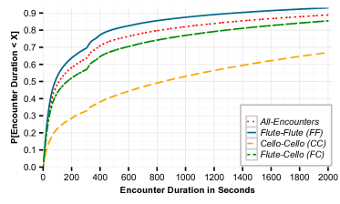
The daily encounter duration based on device types are summarized in Table 3. From the table, it is clear that CC pairs have longer encounter duration than other kinds of pairs. For example, the mean CC daily encounter duration is 290% longer than the FF pairs. This result is beneficial when modeling the encounters based on device type, or with applications that use the encounter duration.
Figure 1 shows the CDF of the encounter duration for 95% of pairs (the highest 5% is omitted for clarity). Note that 80% of FF encounters have daily encounter duration $\leq$8 minutes, while only 40% of CC encounters are $\leq$8 minutes. For all encounters, 33% are $\leq$38s, dubbed short, the next 33% are $\leq$317s, called medium, and $>$317s are long encounters. This definition will be used in Sec. 5 for pairwise analysis of the correlation between encounter duration and traffic profile similarity.

3.2. Encounter Duration Statistical Distributions

Eleven distributions are fit to the total daily encounter duration using maximum likelihood, and goodness-of-fit test methods: Power-law (Pl), Weibull (W), Gamma (G), Lognormal (Ln), Pareto (Pr), Normal (N), Exponential (Ex), Uniform (U), Cauchy (C), Beta (B) and Log-logistic (Ll). The Kolmogorov-Smirnov (KS) statistic is used to evaluate the distributions fitness. The three best-fit distributions are selected and presented in table 4. For example, 74% of the buildings have power-law (Pl) distribution as the best fit for their FF pair daily encounter duration, while only 39% of buildings have CC daily encounter distribution following power-law. Also, table 4 shows the percentage of buildings that have KS-statistic with less than a threshold, specifically $\leq 5\%$ and $\leq 10\%$. This is calculated to see if there is a distribution that can be a good fit for the majority of buildings, even if it is not the first-best fit. Power-law and log-logistic distributions usually have KS-test with $\leq$10% for 92% for FF and FC pairs.

Table 4. Best fit distributions for total daily encounter pairs duration based on pairs classifications. Percentage of buildings shown in brackets. (Pl: Power Law, Ll: Log Logistic, W: Weibull, G: Gamma, Pr: Pareto, Ln: Log Normal, B: Beta).

Pair-Types	1st best fit	2nd best fit	3rd best fit	KS-test¡=5%	KS-test¡=10%
Flute-Flute	Pl[74%], Ll[10%],	Ll[29%], Ln[26%],	Ll[39%], Pr[24%],	Pl[72%], Ll[19%]	Pl[92%], Ll[92%]
(FF)	Pr[8%]	Pr[19%], W[11%]	Ln[21%]	Ln[15%], Pr[15%]	Pr[89%], Ln[85%]
Cello-Cello	Pl[39%], W[21%],	B[22%], Ll[18%]	Ll[25%], W[24%],	Pl[34%], W[32%]	Ll[87%], Pl[86%]
(CC)	B[14%]	Pl[16%], W[14%]	Pr[13%], Pl[12%]	B[30%], G[16%]	W[78%], Ln[71%]
Flute-Cello	Pl[67%], Ll[13%],	Ln[28%], Ll[20%],	Ll[46%], Ln[16%]	Pl[61%], Pr[12%]	Pl[92%], Ll[92%]
(FC)	Pr[9%]	Pr[19%], W[18%], Pl[10%]	Pr[14%]	Ll[11%], W[9%]	Pr[80%],Ln[78%]

4. Web traffic profile

We use NetFlow traces to analyze traffic behavior of user devices. In (Alipour2018, ), we analyzed traffic on an individual level. We found cellos to generate 2x more flows than flutes, while the flute flows are 2.5x larger. Also, flow sizes were found to follow a Lognormal distribution, while flow inter-arrival times (IAT) follow beta distribution, with high skewness/kurtosis, hinting at infrequent extreme values (e.g., flutes incur more extreme periods of inactivity, caused by higher mobility). In this study, we conduct pairwise (vs. individual) level analysis of mobility and traffic.

To analyze traffic patterns of users for all buildings and days, we first define a Traffic Profile (TP) for each user based on NetFlow traces. This traffic profile is efficient to calculate and granular enough for our analysis:

• First, we select a set of popular websites for analysis based on total bytes sent and received, filtering out websites with little usage. The IP address of selected websites form the dimensions of the traffic vector, denoted as $\kappa$. There are $\approx 10,000$ IP addresses in $\kappa$, with average daily traffic from few $MB$s, and up to $690GB$s.

• Next, for each address, $IP_{j}$, we calculate $B_{(i,j)}$, defined as the natural logarithm of total traffic user i, $U_{i}$, has sent to or received from $IP_{j}$. This forms the initial traffic vector for $U_{i}$ , consisting of $B_{(i,j)},\forall j\in\kappa$.

• Finally, we apply term frequency-inverse document frequency (TF-IDF (salton1986introduction, )) to the collection of traffic vectors of all users. This reduces the effect of wildly popular websites, and identifies websites that can distinguish between users’ online behavior, enabling us to study the richness in the access patterns. In this context, each $IP_{j}$ is a term and each user traffic vector is a document. TF-IDF is calculated as the product of term frequency (the number of times a term appears in a document, corresponding to $B_{(i,j)}$ in our context, which reflects the bytes $IP_{j}$ exchanged with $U_{i}$), and inverse document frequency (the inverse of number of documents (users) the term (IP) occurs in) (idf, ). Each row of the resulting matrix is a traffic profile, $TP_{i}$, of user $U_{i}$, as depicted in Fig 2.

  $$\begin{array}[]{cccc}&\text{$\text{IP}_{j}$}\\ \text{\emph{TF-IDF}=}&\begin{bmatrix}&\vdots&\\ <\cdots&B_{i,j}&\cdots>\\ &\vdots&\end{bmatrix}&\text{$\leftarrow$ $TP_{i}$}\end{array}$$

  Figure 2. TF-IDF Matrix: Each row is a user profile.

This process is applied for NetFlow data of every building on each day, to enable spatial (across buildings) and temporal (across days) analysis of user traffic profiles. For pairwise comparison of traffic profiles, we use Cosine similarity which computes the cosine of the angle between two user profiles.

5. Pairwise encounter-traffic relationship

With mobility encounters and traffic profiles as the pillars, here, we take steps to investigate ”whether physical encounters are correlated with the similarity of traffic profiles”. This analysis outlines our initial findings in the pairwise (encounter) dimension of mobility-traffic analysis, following our work in (Alipour2018, ) that focused on individual aspect of combined mobility-traffic modeling, and providing the foundation for collective (group) analysis in the future. We start with simple steps, and increase the complexity of methods gradually.

As a first step, we seek to establish whether the traffic profiles of encountered pairs are more similar compared to traffic profiles of non-encountered pairs of users. For this purpose, we calculate $enc=Sum\sum_{\forall(i,j)\in Z}{\frac{cosine(TP_{i},TP_{j})}{|Z|}}$. Here, $Z$ denotes the set of all encountered pairs of users. Similarly, for all non-encountered pairs, $Z^{\prime}$, $nonenc=Sum\sum_{\forall(i,j)\in Z^{\prime}}{\frac{cosine(TP_{i},TP_{j})}{|Z^{\prime}|}}$. This calculation is carried out on each building every day. Overall, we observe that $\approx$93% of the time enc ¿ nonenc, with the main exceptions being buildings close to bus stop hubs on campus, with a high pass-by rate of users; resulting in many short encounters that do not show traffic similarity. With that simple observation, next, we asked whether the difference between traffic similarity of encountered and non-encountered is statistically significant. Mann–Whitney U test (mann1947test, ) was applied on the two independent sets, with the null hypothesis being the two sets are drawn from the same distribution. We find that for $86\%$ of (building, day) tuples, we can reject the null hypothesis ($p<0.05$). This shows that in most cases, the traffic profiles of encountered pairs are more similar and the difference between the two groups is statistically significant. Logistic regression analysis shows that similarity of traffic profiles is significantly associated with the probability of encountering for all days in several buildings, such as the computer department with a big user base, for $\approx 90\%$ of days in libraries, and only for $\approx 48\%$ of days in gym and recreation centers where users normally do not use networks as much. The next question is how consistent these differences are across:

1. Device type categories: As discussed earlier, usage patterns of devices differ based on form factor (e.g., on-the-go flutes vs. sit-to-use cellos). We compare flute-flute (FF), cello-cello (CC), and flute-cello (FC) encounters.

2. Weekday vs. Weekend: We established significant differences between mobility and traffic patterns of weekdays and weekends in (Alipour2018, ). Here we analyze the mobility encounter-traffic interplay across the weekdays and weekends.

3. Encounter duration: We define three encounter duration categories using 3 bins of equal frequency: short ($<0.6min$), medium ($0.6-5min$) and long ($>5min$). We then analyze each group for correlation between encounter duration and traffic profile similarity.

5.1. Device type categories

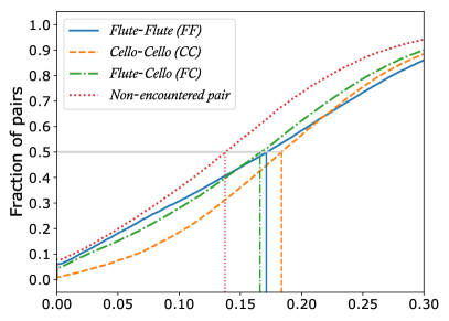
We analyze how similarity of traffic profiles for encountered pairs varies when two flutes meet (FF), two cellos meet (CC) or a flute meets a cello (FC). The results, as presented in Figure 3, show that the similarity of CC is slightly higher than the other groups, while the FF and FC groups show similar trends. Notably, however, all three encountered groups are significantly different from the non-encountered group ($p<0.05$). This is consistent across most buildings. Given the context of the traces, we suspect heavy use of laptops for educational content on campus. Further analysis website content may shed light on the shared interests among encountered users with various forms of devices. We leave this for future work.

Figure 3. CDF of pairwise cosine similarity of traffic profiles across device types (vertical lines denote medians).

5.2. Weekday vs. Weekend

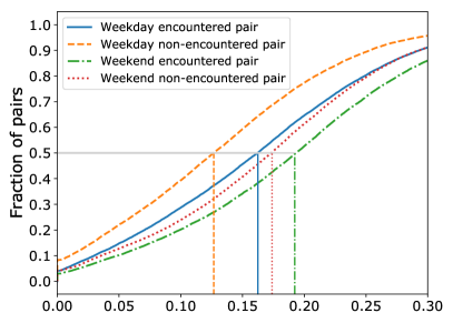
Intuitively, there are significant differences between weekdays and weekends in user behavior, and consequently their mobility and traffic patterns. In (Alipour2018, ), we found that numbers of user devices on campus drops significantly on weekends, but the remaining devices do not show significant differences in terms of flow size, packet count, and active duration. Here we identify and quantify the encounter-traffic correlation over weekdays/weekends for the first time. Results are depicted in Fig 4. We find that the pairwise similarities of weekend pairs to be overall higher than their weekday counterparts regardless of an encounter (or not), with weekend non-encountered pairs being more similar than weekday encountered pairs. This is explained by observing significantly reduced mobility of devices on weekends. For example, median radius of gyration for cellos drops by 66%, and by 15% for flutes (Alipour2018, ). In addition to decreased mobility, most activity is clustered around several academic buildings with research labs (33% of APs handle no flute traffic on weekends, while 56% receive no cello traffic). Thus the increase in traffic similarity during weekends might be explained by the presence of researchers collaborating on related fields of interest and accessing similar content.

Figure 4. CDF of pairwise cosine similarity of traffic profiles in weekdays and weekends (vertical lines denote medians).

5.3. Encounter duration

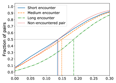
Based on the encounter durations introduced in Section 3.1, we define three encounter duration categories with 3 bins of equal frequency: short ($<0.6min$), medium ($0.6-5min$) and long ($>5min$). As depicted in Fig. 5, the short encounter group is not significantly different from the group of non-encountered pairs ($p>0.05$). However, the differences between the other groups are statistically significant, with the long encounter group showing the highest similarity of traffic profiles, hinting at a correlation between the duration of encounter and traffic profile similarity.

Figure 5. CDF of pairwise cosine similarity of traffic profiles with different encounter durations (vertical lines denote medians).

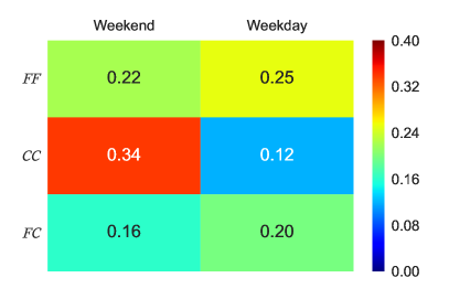
Hence, we investigate this correlation. We found insignificant correlation for short and medium encounters (based on Pearson and Spearman correlation coefficients), however there is a small positive linear correlation between encounter duration and traffic profile similarity for long encounters ($\rho=0.21$). Breaking down the correlations into different device types and weekday/weekend (Fig. 6), shows the highest correlation for Cello-Cello (CC) encounters on weekends, supporting our earlier observation.

Figure 6. Pearson correlation coefficient between encounter duration and traffic profile similarity. (Cello-Cello (CC) encounters on weekends show the highest positive correlation.)

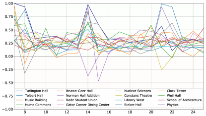
Overall, the correlation between encounter duration and traffic profile similarity is dynamic, changing across space and time. Fig. 7 shows a time-series plot of the linear correlation coefficient of several buildings on campus for more than 3 weeks. It shows how the correlation varies across time in different buildings, with rapid changes every 7 days (around weekends). Surprisingly, a few buildings show significant negative correlations on weekends (e.g., music and theater buildings), while others show significant positive correlations on the same days (mostly academic buildings). Further analysis of the other buildings and its interaction with mobility encounters and traffic profiles are left for future work.

Figure 7. Pearson correlation coefficient between encounter duration and traffic profile similarity for different buildings across days (X-axis).

6. Learning encounters

Given the relationships shown so far, there seems to be great potential in training a machine learning model that can learn to predict an encounter given two traffic profiles. Such a model has several practical applications. Given two traffic profiles, if it is possible to predict they have encountered on a certain day in a building with good accuracy, then there is useful information in the relationship of mobility encounter and traffic profile similarity, which could be used in design of encounter-based dissemination protocols, analysis of rumor anatomy, or tracing of disease spread (inTrace, ) even if mobility traces are not reliable for each user (for example due to MAC address randomization), but traffic profiles of users are accessible (via authentication mechanisms identifying users at a higher OSI layer).

To investigate the feasibility of this task, for every pair of users, their traffic profiles in each building and on each day are coupled as input (either through concatenation or taking the absolute differences, with the former depicted in results and figures), and a binary target label is assigned based on whether the pair has encountered on that day and building. Since most pairs of users do not typically encounter on a day, predicting a negative label is rather trivial in this case. To prevent this bias, we sample this dataset to make sure each label is represented by an equal number of samples for our models.

6.1. Random Forest

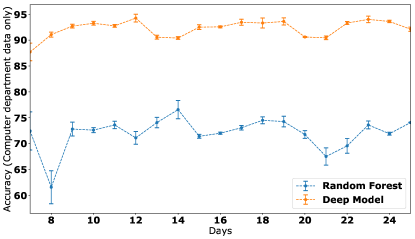
We first used Random Forests (ho1995random, ; Breiman2001, ) for this classification task, which is a well-established algorithm used for supervised learning problems. Our work showed that on a building (the computer department) the algorithm achieved a promising $\approx 70\%$ accuracy on average across all days, based on stratified k-fold cross-validation, without employing any preprocessing or parameter tuning of the model. Next, we applied a dimensionality reduction algorithm, using Singular-Value Decomposition (SVD) to preprocess the input vector. This technique is adapted from Latent semantic analysis of natural language processing. Its application improved the accuracy, in the same settings, to $\approx 73\%$. This lead to the idea of using stacked auto-encoders (SAE) to retain information and connect the SAE to a deep, fully-connected neural network (DNN) for classification.

Figure 8. Accuracy of random forest and deep learning model for encounters in the computer department across days (X-axis).

6.2. Deep learning

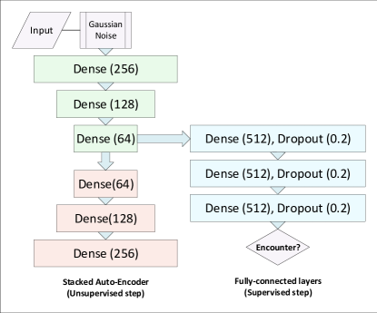
We utilized several recent ideas from the field of artificial intelligence to improve our learning of encounters significantly. Auto-encoders are a class of artificial neural networks that are trained in an unsupervised fashion to learn an efficient representation of their input. In simple terms, the network consists of two stages: encoder and decoder. The encoder consists of layers of decreasing size, that is then connected to the decoder, which is made up of layers of increasing size. The objective is to reconstruct the input as accurately as possible with purely unsupervised learning. Stacked auto-encoders (SAE) have been used in various applications to extract features (masci2011stacked, ), reduce dimensionality (nowicki2017low, ), as well as denoising the corrupted variations of input (vincent2010stacked, ).

We use a Stacked De-noising Auto-Encoder (SDAE) (vincent2010stacked, ). This network is provided with input data corrupted by Gaussian noise, and is trained to reconstruct the original, uncorrupted input similar to a traditional auto-encoder. Thus, denoising becomes a training criterion, while dimensionality reduction of input is also achieved (We kindly refer the reader to (vincent2010stacked, ) for details of SDAE and comparison with SAE). Then, the encoded data points are fed to a fully connected, multi-layer neural network. Comparing the results to the random forest, there is a significant increase in accuracy to an average of 92% for the same building and days as the random forest classifier. Comparing device type categories of encounters, we find cello-cello encounters to be the most distinguishable, followed by flute-cello and flute-flute. However, the difference between accuracies for different device type categories is ¡5% in most locations and dates, a testimony to the robustness of the model. This accuracy is also stable across time, with the median of accuracy, for weekdays at 93.25%, and weekends at 90.75%, for the computer department samples. The much higher accuracy comes at the cost of high compute power costs and complexity of the model. Fig. 8 shows the results of both the random forest and the deep neural network model for this building across $\approx 3$ weeks. We used stratified k-fold cross-validation, early stopping and dropout layers to regularize the network and alleviate overfitting. An illustration of the architecture is presented in Fig. 9.

Figure 9. Architecture of the deep learning model. Numbers show the number of neurons in each layer (internal details omitted for brevity).

7. Conclusions and future work

In this study, we present the first steps to analyze and quantify the relation between mobility and traffic. Focusing on the pairwise (encounter) dimension of mobility, its interplay with the traffic patterns of mobile users was studied. This work has implications for realistic modeling and simulation, offloading through opportunistic encounters, as well as implementation and benchmarking of encounter-based services such as content sharing, mobile social networks and encounter-based trust. We use extensive, highly granular datasets (30TB in size), in more than 140 buildings on a university campus, including information about WiFi associations, DHCP and NetFlow, covering the dimensions of mobility and network traffic.

To answer our main question of ‘How do device encounters affect network traffic patterns, across time, space, device type, and encounter duration?’, We analyze mobility encounters and presented their statistical characteristics. We defined traffic profiles and utilized numerical statistics and machine learning techniques. Power law and Log logistic distributions, fitted to daily encounter duration, have KS-test $\leq$10% in 92% of buildings for Flute-Flute (FF) and Flute-Cello (FC) encounters, and 86% for Cello-Cello (CC) encounters. Also, CC pairs have longer daily encounter duration. Analyzing traffic, we find significant differences between traffic profile similarity of encountered versus non-encountered pairs for device type categories (FF, CC, FC), with the highest similarity being the CC group. Further, comparing weekdays and weekends, in both cases, the encountered pairs are more similar, with the distinction that weekend traffic profiles are more similar than weekdays’. Analysis of correlation between encounter duration and traffic profile similarity revealed short and medium encounters not being significantly different from the non-encountered group, while the long encounters show significantly higher similarity. We also employed random forests and created a deep neural network (DNN) model to predict encounters of pairs of user traffic profiles, with a very high accuracy (up to 94% depending on settings).

The findings in this paper are not currently captured by any of the existing mobility or traffic models, while having important implications in many contexts, such as predictive caching, information dissemination, opportunistic social networks and infection tracing. This provides a compelling case for integrated traffic-mobility models that consider multiple dimensions of social context (individual, pairwise, and group). We plan to further investigate the causal relationship between mobility and traffic for pairwise and collective (group) dimensions in the future. Exploration of applications of our learning methods, its privacy implications, and potential improvements are also left for future work.

References

- (1) F. Bai, N. Sadagopan, and A. Helmy, “The important framework for analyzing the impact of mobility on performance of routing protocols for adhoc networks,” Ad hoc networks, 2003.
- (2) J. Treurniet, “A Taxonomy and Survey of Microscopic Mobility Models from the Mobile Networking Domain,” ACM CSUR, 2014.
- (3) A. Hess, K. A. Hummel, W. N. Gansterer, and G. Haring, “Data-driven Human Mobility Modeling: A Survey and Engineering Guidance for Mobile Networking,” ACM CSUR, 2016.
- (4) G. S. Thakur and A. Helmy, “Cobra: A framework for the analysis of realistic mobility models,” in INFOCOM’13.
- (5) W.-J. Hsu, T. Spyropoulos, K. Psounis, and A. Helmy, “Modeling spatial and temporal dependencies of user mobility in wireless mobile networks,” IEEE/ACM Transactions on Networking (ToN), 2009.
- (6) J. Manweiler, R. Scudellari, and L. P. Cox, “Smile: encounter-based trust for mobile social services,” in Proceedings of the 16th ACM CCS, 2009.
- (7) Y. Dong, Y. Yang, J. Tang, Y. Yang, and N. V. Chawla, “Inferring user demographics and social strategies in mobile social networks,” in Proceedings of the 20th ACM SIGKDD, 2014.
- (8) W.-j. Hsu and A. Helmy, “On nodal encounter patterns in wireless lan traces,” IEEE Transactions on Mobile Computing, 2010.
- (9) A. Chaintreau, P. Hui, J. Crowcroft, C. Diot, R. Gass, and J. Scott, “Impact of human mobility on opportunistic forwarding algorithms,” IEEE Transactions on Mobile Computing, 2007.
- (10) N. Eagle and A. S. Pentland, “Reality mining: sensing complex social systems,” Personal and ubiquitous computing, 2006.
- (11) P. Hui, A. Chaintreau, J. Scott, R. Gass, J. Crowcroft, and C. Diot, “Pocket switched networks and human mobility in conference environments,” in Proceedings of the 2005 ACM SIGCOMM workshop on DTN.
- (12) X. G. Meng, S. H. Wong, Y. Yuan, and S. Lu, “Characterizing flows in large wireless data networks,” MobiCom ’04.
- (13) S. Moghaddam, A. Helmy, S. Ranka, and M. Somaiya, “Data-driven co-clustering model of internet usage in large mobile societies,” ACM MSWiM’10.
- (14) M. Afanasyev, T. Chen, G. M. Voelker, and A. C. Snoeren, “Analysis of a mixed-use urban wifi network: when metropolitan becomes neapolitan,” in ACM SIGCOMM ’08.
- (15) G. Maier, F. Schneider, and A. Feldmann, “A first look at mobile hand-held device traffic,” in PAM ’10. Springer.
- (16) H. Falaki, D. Lymberopoulos, R. Mahajan, S. Kandula, and D. Estrin, “A first look at traffic on smartphones,” ACM IMC ’10.
- (17) X. Chen, R. Jin, K. Suh, B. Wang, and W. Wei, “Network performance of smart mobile handhelds in a university campus wifi network,” ACM IMC’12.
- (18) U. Kumar, J. Kim, and A. Helmy, “Changing patterns of mobile network (WLAN) usage: Smart-phones vs. laptops,” IWCMC ’13.
- (19) A. Gember, A. Anand, and A. Akella, “A comparative study of handheld and non-handheld traffic in campus wi-fi networks,” in PAM ’11.
- (20) I. Papapanagiotou, E. M. Nahum, and V. Pappas, “Smartphones vs. laptops: comparing web browsing behavior and the implications for caching,” SIGMETRICS ’12.
- (21) B. Alipour, L. Tonetto, A. Yi Ding, R. Ketabi, J. Ott, and A. Helmy, “Flutes vs. cellos: Analyzing mobility-traffic correlations in large wlan traces,” in IEEE INFOCOM, 2018.
- (22) M. ElSherief, B. Alipour, M. Al Qathrady, T. ElBatt, A. Zahran, and A. Helmy, “A novel mathematical framework for similarity-based opportunistic social networks,” PMC, 2017.
- (23) M. Al Qathrady, A. Helmy, and K. Almuzaini, “Infection tracing in smart hospitals,” in IEEE WiMob ’16.
- (24) G. Salton and M. J. McGill, “Introduction to modern information retrieval,” 1986.
- (25) K. S. JONES, “A statistical interpretation of term specificity and its application in retrieval,” Journal of Documentation, vol. 28, 1972.
- (26) H. B. Mann and D. R. Whitney, “On a test of whether one of two random variables is stochastically larger than the other,” The annals of mathematical statistics, 1947.
- (27) T. K. Ho, “Random decision forests,” in Document analysis and recognition, 1995., proceedings of the third international conference on, vol. 1. IEEE, 1995, pp. 278–282.
- (28) L. Breiman, “Random forests,” Machine Learning, vol. 45, no. 1, pp. 5–32, 2001.
- (29) J. Masci, U. Meier, D. Cireşan, and J. Schmidhuber, “Stacked convolutional auto-encoders for hierarchical feature extraction,” in International Conference on Artificial Neural Networks. Springer, 2011, pp. 52–59.
- (30) M. Nowicki and J. Wietrzykowski, “Low-effort place recognition with wifi fingerprints using deep learning,” in International Conference Automation. Springer, 2017, pp. 575–584.
- (31) P. Vincent, H. Larochelle, I. Lajoie, Y. Bengio, and P.-A. Manzagol, “Stacked denoising autoencoders: Learning useful representations in a deep network with a local denoising criterion,” Journal of Machine Learning Research, vol. 11, no. Dec, pp. 3371–3408, 2010.
- (32) P. Pons and M. Latapy, “Computing communities in large networks using random walks,” in International symposium on computer and information sciences. Springer, 2005, pp. 284–293.