Low-complexity 8-point DCT Approximation Based on Angle Similarity for Image and Video Coding

Raíza S. Oliveira R. S. Oliveira is with the Programa de Pós-Graduação em Engenharia Elétrica, Universidade Federal de Pernambuco (UFPE), Recife, Brazil; and with the Signal Processing Group, Departamento de Estatística, UFPE.    Renato J. Cintra Renato J. Cintra is with the Signal Processing Group, Departamento de Estatística, Universidade Federal de Pernambuco, Recife, Brazil; ECE, University of Calgary, Calgary, AB, Canada. E-mail: rjdsc@de.ufpe.br    Fábio M. Bayer F. M. Bayer is with the Departamento de Estatística, Universidade Federal de Santa Maria, Santa Maria, and LACESM, Brazil.    Thiago L. T. da Silveira T. L. T. Silveira is with the Programa de Pós-Graduação em Computação, Universidade Federal do Rio Grande do Sul, Porto Alegre, Brazil.    Arjuna Madanayake Arjuna Madanayake is with the Department of Electrical and Computer Engineering, University of Akron, Akron, OH.    André Leite André Leite is with the Departamento de Estatística, Universidade Federal de Pernambuco, Recife, Brazil. E-mail: leite@de.ufpe.br
{onecolabstract}

The principal component analysis (PCA) is widely used for data decorrelation and dimensionality reduction. However, the use of PCA may be impractical in real-time applications, or in situations were energy and computing constraints are severe. In this context, the discrete cosine transform (DCT) becomes a low-cost alternative to data decorrelation. This paper presents a method to derive computationally efficient approximations to the DCT. The proposed method aims at the minimization of the angle between the rows of the exact DCT matrix and the rows of the approximated transformation matrix. The resulting transformations matrices are orthogonal and have extremely low arithmetic complexity. Considering popular performance measures, one of the proposed transformation matrices outperforms the best competitors in both matrix error and coding capabilities. Practical applications in image and video coding demonstrate the relevance of the proposed transformation. In fact, we show that the proposed approximate DCT can outperform the exact DCT for image encoding under certain compression ratios. The proposed transform and its direct competitors are also physically realized as digital prototype circuits using FPGA technology.

Keywords
DCT Approximation, Fast algorithms, Image/video encoding

\saythanks

1 Introduction

Data decorrelation is a central task in many statistical and signal processing problems [1, 2, 3]. Decorrelation can be accomplished by means of a linear transformation that converts correlated observations into linearly uncorrelated values. This operation is commonly performed by principal component analysis (PCA) [2]. PCA is widely used to reduce the dimensionality of data [2, 4], where the information contained in all the original variables is replaced by the data variability information of the initial few uncorrelated principal components. The quality of such approximation depends on the number of components used and the proportion of variance explained, or energy retained, by each of them.

In the field of analysis and processing of images and signals, PCA, also known as the discrete Karhunen–Loève transform (KLT) [3], is considered the optimal linear transformation for data decorrelation when the signal is a first order Markov process [5, 3]. The KLT has the following features [3]: (i) decorrelates the input data completely in the transform domain; (ii) minimizes the mean square error in data compression; and (iii) concentrates the energy (variance) in a few coefficients of the output vector. Because the KLT matrix depends on the variance and covariance matrix of the input data, deriving computationally efficient algorithms for real-time processing becomes a very hard task [6, 7, 8, 9, 10, 11, 12, 3, 13].

If the input data follows a stationary highly correlated first-order Markov process [12, 3, 14], then the KLT is very closely approximated by the discrete cosine transform (DCT) [12, 3]. Natural images fall into this particular statistical model category [15]. Thus DCT inherits the decorrelation and compaction properties of the KLT, with the advantage of having a closed-form expression independent of the input signal. Image and video communities widely adopt the DCT in their most successful compression standards, such as JPEG [16] and MPEG [17]. Often such standards include two-dimensional (2-D) versions of the DCT applied to small image blocks ranging from 4×\times4 to 32×\times32 pixels.

The 8×\times8 block is employed in a large number of standards, for example: JPEG [16], MPEG [18], H.261 [19], H.263 [20], H.264/AVC [21], and HEVC [22]. The arithmetic cost of the 8-point DCT is 64 multiplications and 56 additions, when computed by definition. Fast algorithms can dramatically reduce the arithmetic cost to 11 multiplications and 29 additions, as in the Loeffler DCT algorithm [23].

However, the number of DCT calls in common image and video encoders is extraordinarily high. For instance, a single image frame of high-definition TV (HDTV) contains 32.400 8×\times8 image subblocks. Therefore, computational savings in the DCT step may effect significant performance gains, both in terms of speed and power consumption [24, 25]. Being quite a mature area of research [26], there is little room for improvement on the exact DCT computation. Thus, one approach to further minimize the computational cost of computing the DCT is the use of matrix approximations [27, 14]. Such approximations provide matrices with similar mathematical behavior to the exact DCT while presenting a dramatically low arithmetic cost.

The goals of this paper are as follows. First, we aim at establishing an optimization problem to facilitate the derivation of 8-point DCT approximations. To this end, we adopt a vector angle based objective function to minimize the angle between the rows of the approximate and the exact DCT matrices subject to orthogonality constraints. Second, the sought approximations are (i) submitted to a comprehensive assessment based on well-known figures of merit and (ii) compared to state-of-the-art DCT approximations. Third, fast algorithms are derived and realized in FPGA hardware with comparisons with competing methods. We also examine the performance of the obtained transformations in the context of image compression and video coding. We demonstrate that one of our DCT approximations can outperform the exact DCT in terms of effected quality after image compression.

This paper is organized as follows. In Section 2, the 8-point DCT and popular DCT approximations are discussed. Section 3 introduces an optimization problem to pave the way for the derivation of new DCT approximations. In Section 4 the proposed approximations are detailed and assessed according to well-known performance measures. In Section 5 a fast algorithm for the proposed approximation is presented. Moreover, a field-programmable gate array (FPGA) design is proposed and compared with competing methods. Section 6 furnishes computational evidence of the appropriateness of the introduced approximate DCT for image and video encoding. Section 7 concludes the paper.

2 DCT Approximations

Let 𝐱𝐱\mathbf{x} and 𝐗𝐗\mathbf{X} be 8-point column vectors related by the DCT. Therefore, they satisfy the following expression: 𝐗=𝐂𝐱𝐗𝐂𝐱\mathbf{X}=\mathbf{C}\cdot\mathbf{x}, where

𝐂=[γ3γ3γ3γ3γ3γ3γ3γ3γ0γ2γ4γ6γ6γ4γ2γ0γ1γ5γ5γ1γ1γ5γ5γ1γ2γ6γ0γ4γ4γ0γ6γ2γ3γ3γ3γ3γ3γ3γ3γ3γ4γ0γ6γ2γ2γ6γ0γ4γ5γ1γ1γ5γ5γ1γ1γ5γ6γ4γ2γ0γ0γ2γ4γ6],𝐂delimited-[]subscript𝛾3subscript𝛾3subscript𝛾3subscript𝛾3subscript𝛾3subscript𝛾3subscript𝛾3subscript𝛾3subscript𝛾0subscript𝛾2subscript𝛾4subscript𝛾6subscript𝛾6subscript𝛾4subscript𝛾2subscript𝛾0subscript𝛾1subscript𝛾5subscript𝛾5subscript𝛾1subscript𝛾1subscript𝛾5subscript𝛾5subscript𝛾1subscript𝛾2subscript𝛾6subscript𝛾0subscript𝛾4subscript𝛾4subscript𝛾0subscript𝛾6subscript𝛾2subscript𝛾3subscript𝛾3subscript𝛾3subscript𝛾3subscript𝛾3subscript𝛾3subscript𝛾3subscript𝛾3subscript𝛾4subscript𝛾0subscript𝛾6subscript𝛾2subscript𝛾2subscript𝛾6subscript𝛾0subscript𝛾4subscript𝛾5subscript𝛾1subscript𝛾1subscript𝛾5subscript𝛾5subscript𝛾1subscript𝛾1subscript𝛾5subscript𝛾6subscript𝛾4subscript𝛾2subscript𝛾0subscript𝛾0subscript𝛾2subscript𝛾4subscript𝛾6\displaystyle\mathbf{C}=\left[\begin{smallmatrix}\gamma_{3}&\phantom{-}\gamma_{3}&\phantom{-}\gamma_{3}&\phantom{-}\gamma_{3}&\phantom{-}\gamma_{3}&\phantom{-}\gamma_{3}&\phantom{-}\gamma_{3}&\phantom{-}\gamma_{3}\\ \gamma_{0}&\phantom{-}\gamma_{2}&\phantom{-}\gamma_{4}&\phantom{-}\gamma_{6}&-\gamma_{6}&-\gamma_{4}&-\gamma_{2}&-\gamma_{0}\\ \gamma_{1}&\phantom{-}\gamma_{5}&-\gamma_{5}&-\gamma_{1}&-\gamma_{1}&-\gamma_{5}&\phantom{-}\gamma_{5}&\phantom{-}\gamma_{1}\\ \gamma_{2}&-\gamma_{6}&-\gamma_{0}&-\gamma_{4}&\phantom{-}\gamma_{4}&\phantom{-}\gamma_{0}&\phantom{-}\gamma_{6}&-\gamma_{2}\\ \gamma_{3}&-\gamma_{3}&-\gamma_{3}&\phantom{-}\gamma_{3}&\phantom{-}\gamma_{3}&-\gamma_{3}&-\gamma_{3}&\phantom{-}\gamma_{3}\\ \gamma_{4}&-\gamma_{0}&\phantom{-}\gamma_{6}&\phantom{-}\gamma_{2}&-\gamma_{2}&-\gamma_{6}&\phantom{-}\gamma_{0}&-\gamma_{4}\\ \gamma_{5}&-\gamma_{1}&\phantom{-}\gamma_{1}&-\gamma_{5}&-\gamma_{5}&\phantom{-}\gamma_{1}&-\gamma_{1}&\phantom{-}\gamma_{5}\\ \gamma_{6}&-\gamma_{4}&\phantom{-}\gamma_{2}&-\gamma_{0}&\phantom{-}\gamma_{0}&-\gamma_{2}&\phantom{-}\gamma_{4}&-\gamma_{6}\\ \end{smallmatrix}\right],

and γk=cos(2π(k+1)/32)subscript𝛾𝑘2𝜋𝑘132\gamma_{k}=\cos(2{\pi}(k+1)/32), for k=0,1,,6𝑘016k=0,1,\ldots,6.

Common algorithms for efficient DCT computation include: (i) Yuan et al. [28], (ii) Arai et al. [29], (iii) Chen et al. [30], (iv) Feig–Winograd [31], (v) Lee [32], and (vi) Hou [33]. Table 1 lists the computational costs associated to such methods. The theoretical minimal multiplicative complexity is 11 multiplications [34, 23], which is attained by the Loeffler algorithm [23].

Table 1: Computational cost of the fast algorithms for the DCT
Algorithm Multiplications Additions
Loeffler et al. [23, 35, 36] 11 29
Yuan et al. [28, 37] 12 29
Lee [32, 38, 39] 12 29
Hou [33, 40, 41] 12 29
Arai et al. [29, 35, 42] 13 29
Chen et al. [30, 43, 35] 16 26
Feig–Winograd [31, 44] 22 28

A DCT approximation is a matrix 𝐂^^𝐂\widehat{\mathbf{C}} capable of furnishing 𝐗^=𝐂^𝐱^𝐗^𝐂𝐱\widehat{\mathbf{X}}=\widehat{\mathbf{C}}\cdot\mathbf{x} where 𝐗^𝐗^𝐗𝐗\widehat{\mathbf{X}}\approx\mathbf{X} according to some prescribed criterion, such as matrix proximity or coding performance [3]. In general terms, as shown in [45, 46, 47, 3, 48], 𝐂^^𝐂\widehat{\mathbf{C}} is a real valued matrix which consists of two components: (i) a low-complexity matrix 𝐓𝐓\mathbf{T} and (ii) a diagonal matrix 𝐒𝐒\mathbf{S}. Such matrices are given by:

𝐂^=𝐒𝐓,^𝐂𝐒𝐓\displaystyle\widehat{\mathbf{C}}=\mathbf{S}\cdot\mathbf{T}, (1)

where

𝐒=(𝐓𝐓)1.𝐒superscript𝐓superscript𝐓top1\displaystyle\mathbf{S}=\sqrt{(\mathbf{T}\cdot{\mathbf{T}}^{\top})^{-1}}. (2)

The operation \sqrt{\cdot} is the matrix square root operation [49, 50].

Hereafter low-complexity matrices are referred to as 𝐓subscript𝐓\mathbf{T}_{\ast}, where the subscript \ast indicates the considered method. Also DCT approximations are referred to as 𝐂^subscript^𝐂\hat{\mathbf{C}}_{\ast}. If the subscript is absent, then we refer to a generic low-complexity matrix or DCT approximation.

A traditional DCT approximation is the signed DCT (SDCT) [51] which matrix is obtained according to: 18sgn(𝐂)18sgn𝐂\frac{1}{\sqrt{8}}\cdot\operatorname{sgn}(\mathbf{C}), where sgn()sgn\operatorname{sgn}(\cdot) is the entry-wise signum function. Therefore, in this case, the entries of the associated low-complexity matrix 𝐓SDCT=sgn(𝐂)subscript𝐓SDCTsgn𝐂\mathbf{T}_{\text{SDCT}}=\operatorname{sgn}(\mathbf{C}) are in {0,±1}0plus-or-minus1\{0,\pm 1\}. Thus matrix 𝐓SDCTsubscript𝐓SDCT\mathbf{T}_{\text{SDCT}} is multiplierless.

Notably, in the past few years, several approximations for the DCT have been proposed as, for example, the rounded DCT (RDCT, 𝐓RDCTsubscript𝐓RDCT\mathbf{T}_{\text{RDCT}}[27], the modified RDCT (MRDCT, 𝐓MRDCTsubscript𝐓MRDCT\mathbf{T}_{\text{MRDCT}}[48], the series of approximations proposed by Bouguezel–Ahmad–Swamy (BAS) [52, 53, 54, 55, 56], the Lengwehasatit–Ortega approximation (LO, 𝐓LOsubscript𝐓LO\mathbf{T}_{\text{LO}}[57], the approximation proposed by Pati et al. [58], and the collection of approximations introduced in [14]. Most of these approximations are orthogonal with low computational complexity matrix entries. Essentially, they are matrices defined over the set {0,±1/2,±1,±2}0plus-or-minus12plus-or-minus1plus-or-minus2\{0,\pm 1/2,\pm 1,\pm 2\}, with the multiplication by powers of two implying simple bit-shifting operations.

Such approximations were demonstrated to be competitive substitutes for the DCT and its related integer transformations as shown in [27, 48, 52, 53, 54, 55, 56, 57, 14]. Table 2 illustrates some common integer transformations linked to the DCT approximations.

Table 2: Common 8-point low-complexity matrices associated to DCT approximations
Method Transformation Matrix
𝐓RDCTsubscript𝐓RDCT\mathbf{T}_{\text{RDCT}} [27] [1111111111100111100110011011110111111111110110110110011001111110]delimited-[]1111111111100111100110011011110111111111110110110110011001111110\left[\begin{smallmatrix}1&1&1&1&1&1&1&1\\ 1&1&1&0&0&-1&-1&-1\\ 1&0&0&-1&-1&0&0&1\\ 1&0&-1&-1&1&1&0&-1\\ 1&-1&-1&1&1&-1&-1&1\\ 1&-1&0&1&-1&0&1&-1\\ 0&-1&1&0&0&1&-1&0\\ 0&-1&1&-1&1&-1&1&0\\ \end{smallmatrix}\right]
𝐓BAS-2008bsubscript𝐓BAS-2008b\mathbf{T}_{\text{BAS-2008b}} [52] [1111111111100111111111111010010111111111111001111111111111111111]delimited-[]1111111111100111111111111010010111111111111001111111111111111111\left[\begin{smallmatrix}1&1&1&1&1&1&1&1\\ 1&1&1&0&0&-1&-1&-1\\ 1&1&-1&-1&-1&-1&1&1\\ 1&0&-1&0&0&1&0&-1\\ 1&-1&-1&1&1&-1&-1&1\\ 1&-1&1&0&0&-1&1&-1\\ 1&-1&1&-1&-1&1&-1&1\\ 1&-1&1&-1&1&-1&1&-1\\ \end{smallmatrix}\right]
𝐓LOsubscript𝐓LO\mathbf{T}_{\text{LO}} [57] [111111111110011111212111212110111101111111111101101112111212111201111110]delimited-[]111111111110011111212111212110111101111111111101101112111212111201111110\left[\begin{smallmatrix}1&1&1&1&1&1&1&1\\ 1&1&1&0&0&-1&-1&-1\\ 1&\frac{1}{2}&-\frac{1}{2}&-1&-1&-\frac{1}{2}&\frac{1}{2}&1\\ 1&0&-1&-1&1&1&0&-1\\ 1&-1&-1&1&1&-1&-1&1\\ 1&-1&0&1&-1&0&1&-1\\ \frac{1}{2}&-1&1&-\frac{1}{2}&-\frac{1}{2}&1&-1&\frac{1}{2}\\ 0&-1&1&-1&1&-1&1&0\\ \end{smallmatrix}\right]
𝐓6subscript𝐓6\mathbf{T}_{6} [14] [1111111121100112211221121021120111111111120110211221122101122110]delimited-[]1111111121100112211221121021120111111111120110211221122101122110\left[\begin{smallmatrix}1&1&1&1&1&1&1&1\\ 2&1&1&0&0&-1&-1&-2\\ 2&1&-1&-2&-2&-1&1&2\\ 1&0&-2&-1&1&2&0&-1\\ 1&-1&-1&1&1&-1&-1&1\\ 1&-2&0&1&-1&0&2&-1\\ 1&-2&2&-1&-1&2&-2&1\\ 0&-1&1&-2&2&-1&1&0\\ \end{smallmatrix}\right]
𝐓4subscript𝐓4\mathbf{T}_{4} [14] [1111111111100111111111111011110111111111110110111111111101111110]delimited-[]1111111111100111111111111011110111111111110110111111111101111110\left[\begin{smallmatrix}1&1&1&1&1&1&1&1\\ 1&1&1&0&0&-1&-1&-1\\ 1&1&-1&-1&-1&-1&1&1\\ 1&0&-1&-1&1&1&0&-1\\ 1&-1&-1&1&1&-1&-1&1\\ 1&-1&0&1&-1&0&1&-1\\ 1&-1&1&-1&-1&1&-1&1\\ 0&-1&1&-1&1&-1&1&0\\ \end{smallmatrix}\right]

3 Greedy Approximations

3.1 Optimization Approach

Approximate DCT matrices are often obtained by fully considering the exact DCT matrix 𝐂𝐂\mathbf{C}, including its symmetries [59], fast algorithms [33, 23], parametrizations [31], and numerical properties [28]. Usually the low-complexity component of a DCT approximation is found by solving the following optimization problem:

𝐓=argmin𝐓approx(𝐓,𝐂),𝐓subscriptsuperscript𝐓approxsuperscript𝐓𝐂\displaystyle\mathbf{T}=\arg\min_{\mathbf{T}^{\prime}}\operatorname{approx}(\mathbf{T}^{\prime},\mathbf{C}),

where approx(,)approx\operatorname{approx}(\cdot,\cdot) is a particular approximation assessment function—such as proximity measures and coding performance metrics [3]—and subject to various constraints, such as orthogonality and low-complexity of the candidate matrices 𝐓superscript𝐓\mathbf{T}^{\prime}.

However, the DCT matrix can be understood as a stack of row vectors 𝐜ksuperscriptsubscript𝐜𝑘top\mathbf{c}_{k}^{\top}, k=1,2,,8𝑘128k=1,2,\ldots,8, as follows:

𝐂=[𝐜1𝐜2𝐜3𝐜4𝐜5𝐜6𝐜7𝐜8].𝐂superscriptmatrixsubscript𝐜1subscript𝐜2subscript𝐜3subscript𝐜4subscript𝐜5subscript𝐜6subscript𝐜7subscript𝐜8top\displaystyle\mathbf{C}=\begin{bmatrix}\mathbf{c}_{1}&\mathbf{c}_{2}&\mathbf{c}_{3}&\mathbf{c}_{4}&\mathbf{c}_{5}&\mathbf{c}_{6}&\mathbf{c}_{7}&\mathbf{c}_{8}\end{bmatrix}^{\top}. (3)

In the current work, to derive an approximation for 𝐂𝐂\mathbf{C}, we propose to individually approximate each of its rows in the hope that the set of approximate rows generate a good approximate matrix. Such heuristic can be categorized as a greedy method [60]. Therefore, our goal is to derive a low-complexity integer matrix

𝐓=[𝐭1𝐭2𝐭3𝐭4𝐭5𝐭6𝐭7𝐭8]𝐓superscriptmatrixsubscript𝐭1subscript𝐭2subscript𝐭3subscript𝐭4subscript𝐭5subscript𝐭6subscript𝐭7subscript𝐭8top\displaystyle\mathbf{T}=\begin{bmatrix}\mathbf{t}_{1}&\mathbf{t}_{2}&\mathbf{t}_{3}&\mathbf{t}_{4}&\mathbf{t}_{5}&\mathbf{t}_{6}&\mathbf{t}_{7}&\mathbf{t}_{8}\end{bmatrix}^{\top} (4)

such that its rows 𝐭ksuperscriptsubscript𝐭𝑘top\mathbf{t}_{k}^{\top}, k=1,2,,8𝑘128k=1,2,\ldots,8, satisfy:

𝐭k=argmin𝐭𝒟error(𝐭,𝐜k),k=1,2,,8,formulae-sequencesubscript𝐭𝑘subscript𝐭𝒟error𝐭subscript𝐜𝑘𝑘128\displaystyle\mathbf{t}_{k}=\arg\min_{\mathbf{t}\in\mathcal{D}}\operatorname{error}(\mathbf{t},\mathbf{c}_{k}),\quad k=1,2,\ldots,8, (5)

subject to constraints such as (i) low-complexity of the candidate vector 𝐭𝐭\mathbf{t} and (ii) orthogonality of the resulting matrix 𝐓𝐓\mathbf{T}. The objective function error(,)error\operatorname{error}(\cdot,\cdot) returns a given error measure and 𝒟𝒟\mathcal{D} is a suitable search space.

3.2 Search Space

In order to obtain a low-complexity matrix 𝐓𝐓\mathbf{T}, its entries must be computationally simple [3, 11]. We define the search space as the collection of 8-point vectors whose entries are in a set, say 𝒫𝒫\mathcal{P}, of low-complexity elements. Therefore, we have the search space 𝒟=𝒫8𝒟superscript𝒫8\mathcal{D}=\mathcal{P}^{8}. Some choices for 𝒫𝒫\mathcal{P} include: 𝒫1={0,±1}subscript𝒫10plus-or-minus1\mathcal{P}_{1}=\{0,\pm 1\} and 𝒫2={0,±1,±2}subscript𝒫20plus-or-minus1plus-or-minus2\mathcal{P}_{2}=\{0,\pm 1,\pm 2\}. Tables 3 and 4 display some elements of the search spaces 𝒟1=𝒫18subscript𝒟1superscriptsubscript𝒫18\mathcal{D}_{1}=\mathcal{P}_{1}^{8} and 𝒟2=𝒫28subscript𝒟2superscriptsubscript𝒫28\mathcal{D}_{2}=\mathcal{P}_{2}^{8}. These search spaces have 6,561 and 390,625 elements, respectively.

Table 3: Examples of approximated vectors for the search space 𝒟1subscript𝒟1\mathcal{D}_{1}
n𝑛n Approximated Vector
1 [11111111]superscriptmatrix11111111top\begin{bmatrix}1&1&1&1&1&1&1&1\end{bmatrix}^{\top}
2 [11111111]superscriptmatrix11111111top\begin{bmatrix}1&1&1&1&1&1&1&-1\end{bmatrix}^{\top}
3 [11111110]superscriptmatrix11111110top\begin{bmatrix}1&1&1&1&1&1&1&0\end{bmatrix}^{\top}
4 [11111111]superscriptmatrix11111111top\begin{bmatrix}1&1&1&1&1&1&-1&1\end{bmatrix}^{\top}
6558 [11111111]superscriptmatrix11111111top\begin{bmatrix}-1&-1&-1&-1&-1&-1&1&-1\end{bmatrix}^{\top}
6559 [11111111]superscriptmatrix11111111top\begin{bmatrix}-1&-1&-1&-1&-1&-1&-1&1\end{bmatrix}^{\top}
6560 [11111110]superscriptmatrix11111110top\begin{bmatrix}-1&-1&-1&-1&-1&-1&-1&0\end{bmatrix}^{\top}
6561 [11111111]superscriptmatrix11111111top\begin{bmatrix}-1&-1&-1&-1&-1&-1&-1&-1\end{bmatrix}^{\top}
Table 4: Examples of approximated vectors for the search space 𝒟2subscript𝒟2\mathcal{D}_{2}
n𝑛n Approximated Vector
1 [22222221]superscriptmatrix22222221top\begin{bmatrix}2&2&2&2&2&2&2&-1\end{bmatrix}^{\top}
2 [22222220]superscriptmatrix22222220top\begin{bmatrix}2&2&2&2&2&2&2&0\end{bmatrix}^{\top}
3 [22222221]superscriptmatrix22222221top\begin{bmatrix}2&2&2&2&2&2&2&1\end{bmatrix}^{\top}
4 [22222222]superscriptmatrix22222222top\begin{bmatrix}2&2&2&2&2&2&2&2\end{bmatrix}^{\top}
390622 [22222222]superscriptmatrix22222222top\begin{bmatrix}-2&-2&-2&-2&-2&-2&-2&-2\end{bmatrix}^{\top}
390623 [22222221]superscriptmatrix22222221top\begin{bmatrix}-2&-2&-2&-2&-2&-2&-2&-1\end{bmatrix}^{\top}
390624 [22222221]superscriptmatrix22222221top\begin{bmatrix}-2&-2&-2&-2&-2&-2&-2&1\end{bmatrix}^{\top}
390625 [22222220]superscriptmatrix22222220top\begin{bmatrix}-2&-2&-2&-2&-2&-2&-2&0\end{bmatrix}^{\top}

3.3 Objective Function

The problem posed in (5) requires the identification of an error function to quantify the “distance” between the candidate row vectors from 𝒟𝒟\mathcal{D} and the rows of the exact DCT. Related literature often consider error functions based on matrix norms [46], proximity to orthogonality [61], and coding performance [3].

In this work, we propose the utilization of a distance based on the angle between vectors as the objective function to be minimized. Let 𝐮𝐮\mathbf{u} and 𝐯𝐯\mathbf{v} be two vectors defined over the same Euclidean space. The angle between vectors is simply given by:

angle(𝐮,𝐯)=arccos(𝐮,𝐯𝐮𝐯),angle𝐮𝐯𝐮𝐯norm𝐮norm𝐯\displaystyle\operatorname{angle}(\mathbf{u},\mathbf{v})=\arccos\left(\frac{\langle\mathbf{u},\mathbf{v}\rangle}{\|\mathbf{u}\|\cdot\|\mathbf{v}\|}\right),

where ,\langle\cdot,\cdot\rangle is the inner product and \|\cdot\| indicates the norm induced by the inner product [62].

3.4 Orthogonality and Row Order

In addition, we require that the ensemble of rows 𝐭ksuperscriptsubscript𝐭𝑘top\mathbf{t}_{k}^{\top}, k=1,2,,8𝑘128k=1,2,\ldots,8, must form an orthogonal set. This is to ensure that an orthogonal approximation can be obtained. As shown in [45, 47], for this property to be satisfied, it suffices that:

𝐓𝐓=[diagonal matrix].𝐓superscript𝐓topdelimited-[]diagonal matrix\displaystyle\mathbf{T}\cdot\mathbf{T}^{\top}=[\text{diagonal matrix}].

Because we aim at approximating each of the exact DCT matrix rows individually, the row sequential order according to which the approximations are performed may matter. Notice that we approximate the rows of the DCT based on a set of low-complexity rows, the search space. For instance, let us assume that we approximate the rows in the following order: =(1,2,3,4,5,6,7,8)Weierstrass-p12345678\bm{\wp}\leavevmode\nobreak\ =\leavevmode\nobreak\ (1,2,3,4,5,6,7,8). Once we find a good approximate row for the first exact row, i.e., a row vector in the search space which has the smallest angle in relation to that exact row, the second row is approximated considering only the row vectors in the search space that are orthogonal to the approximation for the first row. After that, the third exact row is approximated considering only the row vectors in the search space that are orthogonal to the first and second rows already chosen. And so on. This procedure characterize the greedy nature of the proposed algorithm.

Consider now the approximation order (4,3,5,6,1,2,7,8)43561278(4,3,5,6,1,2,7,8), a permutation of Weierstrass-p\bm{\wp}. In this case, we start by approximating the fourth exact row considering the whole search space because we are starting from it. Hence, the obtained approximate row might be different from the one obtained by considering Weierstrass-p\bm{\wp}, since in that case the search space is restricted in a different manner.

As an example, consider the DCT matrix of length 8, introduced in Section 2 of the manuscript. If considering the low complexity set {1,0,1}101\{-1,0,1\} and the approximation order (1, 2, 3, 4, 5, 6, 7, 8) we obtain the following approximate matrix:

[1111111111100111100110011011110111111111110110110110011001111110].delimited-[]1111111111100111100110011011110111111111110110110110011001111110\displaystyle\left[\begin{smallmatrix}1&\phantom{-}1&\phantom{-}1&\phantom{-}1&\phantom{-}1&\phantom{-}1&\phantom{-}1&\phantom{-}1\\ 1&\phantom{-}1&\phantom{-}1&\phantom{-}0&\phantom{-}0&-1&-1&-1\\ 1&\phantom{-}0&\phantom{-}0&-1&-1&\phantom{-}0&\phantom{-}0&\phantom{-}1\\ 1&\phantom{-}0&-1&-1&\phantom{-}1&\phantom{-}1&\phantom{-}0&-1\\ 1&-1&-1&\phantom{-}1&\phantom{-}1&-1&-1&\phantom{-}1\\ 1&-1&\phantom{-}0&\phantom{-}1&-1&\phantom{-}0&\phantom{-}1&-1\\ 0&-1&\phantom{-}1&\phantom{-}0&\phantom{-}0&\phantom{-}1&-1&\phantom{-}0\\ 0&-1&\phantom{-}1&-1&\phantom{-}1&-1&\phantom{-}1&\phantom{-}0\\ \end{smallmatrix}\right].

In other hand, if we consider the reverse approximation order, (8, 7, 6, 5, 4, 3, 2, 1), we obtain the following matrix:

[1111111111100111111111111011110111111111110110111111111101111110].delimited-[]1111111111100111111111111011110111111111110110111111111101111110\displaystyle\left[\begin{smallmatrix}1&\phantom{-}1&\phantom{-}1&\phantom{-}1&\phantom{-}1&\phantom{-}1&\phantom{-}1&\phantom{-}1\\ 1&\phantom{-}1&\phantom{-}1&\phantom{-}0&\phantom{-}0&-1&-1&-1\\ 1&\phantom{-}1&-1&-1&-1&-1&\phantom{-}1&\phantom{-}1\\ 1&\phantom{-}0&-1&-1&\phantom{-}1&\phantom{-}1&\phantom{-}0&-1\\ 1&-1&-1&\phantom{-}1&\phantom{-}1&-1&-1&\phantom{-}1\\ 1&-1&\phantom{-}0&\phantom{-}1&-1&\phantom{-}0&\phantom{-}1&-1\\ 1&-1&\phantom{-}1&-1&-1&\phantom{-}1&-1&\phantom{-}1\\ 0&-1&\phantom{-}1&-1&\phantom{-}1&-1&\phantom{-}1&\phantom{-}0\\ \end{smallmatrix}\right].

Therefore, the row sequence considered matters for the resulting matrix. The sequence matters during the process of finding the approximate matrix.

Thus, the row vectors 𝐜ksuperscriptsubscript𝐜𝑘top\mathbf{c}_{k}^{\top} from the exact matrix must be approximated in all possibles sequences. For a systematic procedure, all the 8!=403208403208!=40320 possible permutations of the sequence Weierstrass-p\wp must be considered. Let msubscriptWeierstrass-p𝑚\bm{\wp}_{m}, m=1,2,,40320𝑚1240320m=1,2,\ldots,40320, be the resultant sequence that determines the m𝑚mth permutation; e.g. 1250=(1,3,7,6,5,4,8,2)subscriptWeierstrass-p125013765482\bm{\wp}_{1250}=(1,3,7,6,5,4,8,2). The particular elements of a sequence are denoted by m(k)subscriptWeierstrass-p𝑚𝑘\bm{\wp}_{m}(k), k=1,2,,8𝑘128k=1,2,\ldots,8. Then, for the given example above, we have 1250(2)=3subscriptWeierstrass-p125023\bm{\wp}_{1250}(2)=3.

3.5 Proposed Optimization Problem

Considering the above discussion, we can re-cast (5) in more precise terms. For each permutation sequence msubscriptWeierstrass-p𝑚\bm{\wp}_{m}, we have the following optimization problem:

𝐭m(k)=argmin𝐝𝒟angle(𝐜m(k),𝐝),k=1,2,,8,formulae-sequencesubscript𝐭subscriptWeierstrass-p𝑚𝑘subscript𝐝𝒟anglesubscript𝐜subscriptWeierstrass-p𝑚𝑘𝐝𝑘128\displaystyle\mathbf{t}_{\bm{\wp}_{m}(k)}=\arg\min_{\mathbf{d}\in\mathcal{D}}\operatorname{angle}(\mathbf{c}_{\bm{\wp}_{m}(k)},\mathbf{d}),\quad k=1,2,\ldots,8, (6)

subject to:

𝐭m(i),𝐭m(j)=0,ij,formulae-sequencesubscript𝐭subscriptWeierstrass-p𝑚𝑖subscript𝐭subscriptWeierstrass-p𝑚𝑗0𝑖𝑗\displaystyle\langle\mathbf{t}_{\bm{\wp}_{m}(i)},\mathbf{t}_{\bm{\wp}_{m}(j)}\rangle=0,\quad i\neq j,

m=1,2,,40320𝑚1240320m=1,2,\ldots,40320 and a fixed search space 𝒟{𝒟1,𝒟2}𝒟subscript𝒟1subscript𝒟2\mathcal{D}\in\{\mathcal{D}_{1},\mathcal{D}_{2}\}. For each m𝑚m, the solution of the above problem returns eight vectors, 𝐭m(1),𝐭m(2),,𝐭m(8)superscriptsubscript𝐭subscriptWeierstrass-p𝑚1topsuperscriptsubscript𝐭subscriptWeierstrass-p𝑚2topsuperscriptsubscript𝐭subscriptWeierstrass-p𝑚8top\mathbf{t}_{\bm{\wp}_{m}(1)}^{\top},\mathbf{t}_{\bm{\wp}_{m}(2)}^{\top},\ldots,\mathbf{t}_{\bm{\wp}_{m}(8)}^{\top}, that are used as the rows of the desired low-complexity matrix. Note that each sequence msubscriptWeierstrass-p𝑚\bm{\wp}_{m} may result in a different solution. Effectively, there are 8!=403208403208!=40320 problems to be solved. In principle, each permutation msubscriptWeierstrass-p𝑚\bm{\wp}_{m} can furnish a different matrix.

Because the search space is relatively small, we solved (6) by means of exhaustive search. Although simple, such approach ensures the attainment of a solution and avoids convergence issues [60]. Figure 1 shows the pseudo-code for the adopted procedure to solve (6). It is important to highlight that although the proposed formulation is applicable to arbitrary transform lengths, it may not be computationally feasible. For this reason, we restrict our analysis to the 8-point case. Section 6.2 discusses an alternative form of generating higher order DCT approximations.

1:procedure abmApprox(𝐂𝐂\mathbf{C}, Weierstrass-p\bm{\wp}, 𝒟𝒟\mathcal{D})
2:     approximationsapproximationsabsent\textbf{approximations}\leftarrow null 3D matrix of size 8×8×n88𝑛8\times 8\times n;
3:     for m1,||𝑚1Weierstrass-pm\leftarrow 1,|\bm{\wp}| do
4:         m(m,:)subscriptWeierstrass-p𝑚Weierstrass-p𝑚:\bm{\wp}_{m}\leftarrow\bm{\wp}(m,:)
5:         for k1,2,,8𝑘128k\leftarrow 1,2,\ldots,8 do
6:              θmin2πsubscript𝜃𝑚𝑖𝑛2𝜋\theta_{min}\leftarrow 2\pi;
7:              index1𝑖𝑛𝑑𝑒𝑥1index\leftarrow 1;
8:              for i1,2,,|𝒟|𝑖12𝒟i\leftarrow 1,2,\ldots,|\mathcal{D}| do
9:                  auxapproximations(:,:,m)(𝒟(i,:))𝑎𝑢𝑥approximations::𝑚superscript𝒟𝑖:topaux\leftarrow\textbf{approximations}(:,:,m)\cdot(\mathcal{D}(i,:))^{\top}
10:                  if sum(aux)=0sum𝑎𝑢𝑥0\operatorname{sum}(aux)=0 then
11:                       θangle(𝐂(m(k),:),𝒟(i,:));𝜃angle𝐂subscriptWeierstrass-p𝑚𝑘:𝒟𝑖:\theta\leftarrow\operatorname{angle}(\mathbf{C}(\bm{\wp}_{m}(k),:),\mathcal{D}(i,:));
12:                       if θ<θmin𝜃subscript𝜃𝑚𝑖𝑛\theta<\theta_{min} then
13:                           θminθsubscript𝜃𝑚𝑖𝑛𝜃\theta_{min}\leftarrow\theta;
14:                           indexi𝑖𝑛𝑑𝑒𝑥𝑖index\leftarrow i;
15:                       end if
16:                  end if
17:              end for
18:              approximations(m(k),:m)𝒟(index,:)\textbf{approximations}(\bm{\wp}_{m}(k),:m)\leftarrow\mathcal{D}(index,:);
19:         end for
20:     end for
21:end procedure
Figure 1: Algorithm for the proposed method.

4 Results and Evaluation

In this section, we apply the proposed method aiming at the derivation of new approximations for the 8-point DCT. Subsequently, we analyze and compare the obtained matrices with a representative set of DCT approximations described in the literature according to several well-known figures of merit [63].

4.1 New 8-point DCT Approximations

Considering the search spaces 𝒟1subscript𝒟1\mathcal{D}_{1} and 𝒟2subscript𝒟2\mathcal{D}_{2} (cf. Table 3 and Table 4, respectively), we apply the proposed algorithm to solve (6). Because the first and fifth rows of the exact DCT are trivially approximated by the row vectors [11111111]matrix11111111\begin{bmatrix}1&1&1&1&1&1&1&1\end{bmatrix} and [11111111]matrix11111111\begin{bmatrix}1&-1&-1&1&1&-1&-1&1\end{bmatrix}, respectively, we limited the search to the remaining six rows. As a consequence, the number of possible candidate matrices is reduced to 6!=72067206!=720. For 𝒟1subscript𝒟1\mathcal{D}_{1}, only two different matrices were obtained, which coincide with previously archived approximations, namely: (i) the RDCT [27] and (ii) the matrix 𝐓4subscript𝐓4\mathbf{T}_{4} introduced in [14]. These approximations are depicted in Table 2.

On the other hand, considering the search space 𝒟2subscript𝒟2\mathcal{D}_{2}, the following two new matrices were obtained:

𝐓1=[1111111122100122211221121022220111111111220110221221122101222210],subscript𝐓1delimited-[]1111111122100122211221121022220111111111220110221221122101222210\displaystyle\mathbf{T}_{1}=\left[\begin{smallmatrix}1&\phantom{-}1&\phantom{-}1&\phantom{-}1&\phantom{-}1&\phantom{-}1&\phantom{-}1&\phantom{-}1\\ 2&\phantom{-}2&\phantom{-}1&\phantom{-}0&\phantom{-}0&-1&-2&-2\\ 2&\phantom{-}1&-1&-2&-2&-1&\phantom{-}1&\phantom{-}2\\ 1&\phantom{-}0&-2&-2&\phantom{-}2&\phantom{-}2&\phantom{-}0&-1\\ 1&-1&-1&\phantom{-}1&\phantom{-}1&-1&-1&\phantom{-}1\\ 2&-2&\phantom{-}0&\phantom{-}1&-1&\phantom{-}0&\phantom{-}2&-2\\ 1&-2&\phantom{-}2&-1&-1&\phantom{-}2&-2&\phantom{-}1\\ 0&-1&\phantom{-}2&-2&\phantom{-}2&-2&\phantom{-}1&\phantom{-}0\\ \end{smallmatrix}\right],
𝐓2=[1111111121200212211221122021120211111111120220211221122102122120].subscript𝐓2delimited-[]1111111121200212211221122021120211111111120220211221122102122120\displaystyle\mathbf{T}_{2}=\left[\begin{smallmatrix}1&\phantom{-}1&\phantom{-}1&\phantom{-}1&\phantom{-}1&\phantom{-}1&\phantom{-}1&\phantom{-}1\\ 2&\phantom{-}1&\phantom{-}2&\phantom{-}0&\phantom{-}0&-2&-1&-2\\ 2&\phantom{-}1&-1&-2&-2&-1&\phantom{-}1&\phantom{-}2\\ 2&\phantom{-}0&-2&-1&\phantom{-}1&\phantom{-}2&\phantom{-}0&-2\\ 1&-1&-1&\phantom{-}1&\phantom{-}1&-1&-1&\phantom{-}1\\ 1&-2&\phantom{-}0&\phantom{-}2&-2&\phantom{-}0&\phantom{-}2&-1\\ 1&-2&\phantom{-}2&-1&-1&\phantom{-}2&-2&\phantom{-}1\\ 0&-2&\phantom{-}1&-2&\phantom{-}2&-1&\phantom{-}2&\phantom{-}0\\ \end{smallmatrix}\right].

According to (1) and (2), the above low-complexity matrices 𝐓1subscript𝐓1\mathbf{T}_{1} and 𝐓2subscript𝐓2\mathbf{T}_{2} can be modified to provide orthogonal transformations 𝐂^1subscript^𝐂1\widehat{\mathbf{C}}_{1} and 𝐂^2subscript^𝐂2\widehat{\mathbf{C}}_{2}. The selected orthogonalization procedure is based on the polar decomposition as described in [45, 47, 64]. Thus, the orthogonal DCT approximations associated to the matrices 𝐓1subscript𝐓1\mathbf{T}_{1} and 𝐓2subscript𝐓2\mathbf{T}_{2} are given by

𝐂^1=𝐒1𝐓1and𝐂^2=𝐒2𝐓2,formulae-sequencesubscript^𝐂1subscript𝐒1subscript𝐓1andsubscript^𝐂2subscript𝐒2subscript𝐓2\displaystyle\widehat{\mathbf{C}}_{1}=\mathbf{S}_{1}\cdot\mathbf{T}_{1}\quad\text{and}\quad\widehat{\mathbf{C}}_{2}=\mathbf{S}_{2}\cdot\mathbf{T}_{2},

where

𝐒i=(𝐓i𝐓i)1,i=1,2.formulae-sequencesubscript𝐒𝑖superscriptsubscript𝐓𝑖superscriptsubscript𝐓𝑖top1𝑖12\displaystyle\mathbf{S}_{i}=\sqrt{(\mathbf{T}_{i}\cdot{\mathbf{T}_{i}}^{\top})^{-1}},\quad i=1,2.

Thus, it follows that:

𝐒1subscript𝐒1\displaystyle\mathbf{S}_{1} =𝐒2=diag(18,118,120,118,18,118,120,118).absentsubscript𝐒2diag1811812011818118120118\displaystyle=\mathbf{S}_{2}=\operatorname{diag}\left(\frac{1}{\sqrt{8}},\frac{1}{\sqrt{18}},\frac{1}{\sqrt{20}},\frac{1}{\sqrt{18}},\frac{1}{\sqrt{8}},\frac{1}{\sqrt{18}},\frac{1}{\sqrt{20}},\frac{1}{\sqrt{18}}\right).

Other simulations were performed considering extended sets of elements. In particular, following sets were considered: {0,±1,±4}0plus-or-minus1plus-or-minus4\{0,\pm 1,\pm 4\}, {0,±1,±8}0plus-or-minus1plus-or-minus8\{0,\pm 1,\pm 8\}, {0,±1,±2,±4}0plus-or-minus1plus-or-minus2plus-or-minus4\{0,\pm 1,\pm 2,\pm 4\}, {0,±1,±2,±8}0plus-or-minus1plus-or-minus2plus-or-minus8\{0,\pm 1,\pm 2,\pm 8\}, and {0,±2,±4,±8}0plus-or-minus2plus-or-minus4plus-or-minus8\{0,\pm 2,\pm 4,\pm 8\}. Generally, the resulting matrices did not perform as well as the ones being proposed. Moreover, the associate computational cost was consistently higher.

The number of vectors in the search space can be calculated as |𝒟|=|𝒫|8𝒟superscript𝒫8|\mathcal{D}|=|\mathcal{P}|^{8} (cf. Section 3.2). Therefore, including more elements to 𝒫𝒫\mathcal{P} effects a noticeable increase in the size of the search space. As a consequence, the processing time to derive all the 6!66! candidate matrices increases accordingly.

4.2 Approximation Measures

Approximations measurements are computed between an approximate matrix 𝐂^^𝐂\hat{\mathbf{C}} (not the low-complexity matrix 𝐓𝐓\mathbf{T}) relative to the exact DCT. To evaluate the performance of the proposed approximations, 𝐂^1subscript^𝐂1\widehat{\mathbf{C}}_{1} and 𝐂^2subscript^𝐂2\widehat{\mathbf{C}}_{2}, we selected traditional figures of merit: (i) total error energy (ϵ()italic-ϵ\epsilon(\cdot)[46]; (ii) mean square error (MSE()MSE\operatorname{MSE}(\cdot)[3, 65]; (iii) coding gain (Cg()subscript𝐶𝑔C_{g}(\cdot)[3, 66, 67]; and (iv) transform efficiency (η()𝜂\eta(\cdot)[3]. The MSE and total error energy are suitable measures to quantify the difference between the exact DCT and its approximations [3]. The coding gain and transform efficiency are appropriate tools to quantify compression, redundancy removal, and data decorrelation capabilities [3]. Additionally, due the angular nature of the objective function required by the proposed optimization problem, we also considered descriptive circular statistics [68, 69]. Circular statistics allows the quantification of approximation error in terms of the angle difference between the row vectors of the approximated and exact matrix.

Hereafter we adopt the following quantities and notation: the interpixel correlation is ρ=0.95𝜌0.95\rho=0.95 [3, 66, 35], 𝐂^^𝐂\widehat{\mathbf{C}} is an approximation for the DCT, and 𝐑^𝐲=𝐂^𝐑𝐱𝐂^subscript^𝐑𝐲^𝐂subscript𝐑𝐱superscript^𝐂top\widehat{\mathbf{R}}_{\mathbf{y}}=\widehat{\mathbf{C}}\cdot\mathbf{R_{x}}\cdot\widehat{\mathbf{C}}^{\top}, where 𝐑𝐱subscript𝐑𝐱\mathbf{R_{x}} is the covariance matrix of 𝐱𝐱\mathbf{x}, whose elements are given by ρ|ij|superscript𝜌𝑖𝑗\rho^{|i-j|}, i,j=1,2,,8formulae-sequence𝑖𝑗128i,j=1,2,\ldots,8. We detail each of these measures below.

4.2.1 Total Energy Error

The total energy error is a similarity measure given by [46]:

ϵ(𝐂^)=π𝐂𝐂^F2,italic-ϵ^𝐂𝜋superscriptsubscriptnorm𝐂^𝐂F2\displaystyle\epsilon(\widehat{\mathbf{C}})=\pi\cdot\|\mathbf{C}-\widehat{\mathbf{C}}\|_{\text{F}}^{2},

where F\|\cdot\|_{\text{F}} represents the Frobenius norm [70].

4.2.2 Mean Square Error

The MSE of a given approximation 𝐂^^𝐂\widehat{\mathbf{C}} is furnished by [3, 65]:

MSE(𝐂^)=18tr((𝐂𝐂^)𝐑𝐱(𝐂𝐂^)).MSE^𝐂18tr𝐂^𝐂subscript𝐑𝐱superscript𝐂^𝐂top\displaystyle\operatorname{MSE}(\widehat{\mathbf{C}})=\frac{1}{8}\cdot\operatorname{tr}\left((\mathbf{C}-\widehat{\mathbf{C}})\cdot\mathbf{R_{x}}\cdot(\mathbf{C}-\widehat{\mathbf{C}})^{\top}\right).

where tr()tr\operatorname{tr}(\cdot) represents the trace operator [3]. The total energy error and the mean square error are appropriate measures for capturing the approximation error in a Euclidean distance sense.

4.2.3 Coding Gain

The coding gain quantifies the energy compaction capability and is given by [3]:

Cg(𝐂^)=10log10{18i=18ri,i(i=18ri,i𝐜^i2)1/8},subscript𝐶𝑔^𝐂10subscript1018superscriptsubscript𝑖18subscript𝑟𝑖𝑖superscriptsuperscriptsubscriptproduct𝑖18subscript𝑟𝑖𝑖superscriptnormsubscript^𝐜𝑖218\displaystyle C_{g}(\widehat{\mathbf{C}})=10\cdot\log_{10}\left\{\frac{\frac{1}{8}\sum_{i=1}^{8}r_{i,i}}{\left(\prod_{i=1}^{8}r_{i,i}\cdot\|\widehat{\mathbf{c}}_{i}\|^{2}\right)^{1/8}}\right\},

where ri,isubscript𝑟𝑖𝑖r_{i,i} is the i𝑖ith element of the diagonal of 𝐑^𝐲subscript^𝐑𝐲\widehat{\mathbf{R}}_{\mathbf{y}} [3] and 𝐜^isuperscriptsubscript^𝐜𝑖top\widehat{\mathbf{c}}_{i}^{\top} is the i𝑖ith row of 𝐂^^𝐂\widehat{\mathbf{C}}.

However, as pointed in [67], the previous definition is suitable for orthogonal transforms only. For non-orthogonal transforms, such as SDCT [51] and MRDCT [48], we adopt the unified coding gain [67]. For i=1,2,,8𝑖128i=1,2,\ldots,8, let 𝐜^isuperscriptsubscript^𝐜𝑖top\widehat{\mathbf{c}}_{i}^{\top} and 𝐠^isuperscriptsubscript^𝐠𝑖top\widehat{\mathbf{g}}_{i}^{\top} be i𝑖ith row of 𝐂^^𝐂\widehat{\mathbf{C}} and 𝐂^1superscript^𝐂1\widehat{\mathbf{C}}^{-1}, respectively. Then, the unified coding gain is given by:

Cg(𝐂^)=10log10{i=181AiBi8},subscriptsuperscript𝐶𝑔^𝐂10subscript10superscriptsubscriptproduct𝑖1818subscript𝐴𝑖subscript𝐵𝑖\displaystyle C^{*}_{g}(\widehat{\mathbf{C}})=10\cdot\log_{10}\left\{\prod_{i=1}^{8}\frac{1}{\sqrt[8]{A_{i}\cdot B_{i}}}\right\},

where Ai=su[(𝐜^i𝐜^i)𝐑x],subscript𝐴𝑖sudirect-productsubscript^𝐜𝑖superscriptsubscript^𝐜𝑖topsubscript𝐑𝑥A_{i}=\operatorname{su}\left[\left(\widehat{\mathbf{c}}_{i}\cdot\widehat{\mathbf{c}}_{i}^{\top}\right)\odot\mathbf{R}_{x}\right], su()su\operatorname{su}(\cdot) returns the sum of all elements of the input matrix, the operator direct-product\odot represents the element-wise product, and Bi=𝐠^i2subscript𝐵𝑖superscriptnormsubscript^𝐠𝑖2B_{i}=\|\widehat{\mathbf{g}}_{i}\|^{2}.

4.2.4 Transform Efficiency

The transform efficiency is an alternative measure to the coding gain, being expressed according to [3]:

η(𝐂^)=i=18|ri,i|i=18j=18|ri,j|100,𝜂^𝐂superscriptsubscript𝑖18subscript𝑟𝑖𝑖superscriptsubscript𝑖18superscriptsubscript𝑗18subscript𝑟𝑖𝑗100\displaystyle\eta(\widehat{\mathbf{C}})=\frac{\sum_{i=1}^{8}|r_{i,i}|}{\sum_{i=1}^{8}\sum_{j=1}^{8}|r_{i,j}|}\cdot 100,

where ri,jsubscript𝑟𝑖𝑗r_{i,j} is the (i,j)𝑖𝑗(i,j)th entry of 𝐑^𝐲subscript^𝐑𝐲\widehat{\mathbf{R}}_{\mathbf{y}}, i,j=1,2,,8formulae-sequence𝑖𝑗128i,j=1,2,\ldots,8 [3].

4.2.5 Circular Statistics

Because the objective function in (6) is the operator angle, its associate values are distributed around the unit circle. This type of data is suitably analyzed by circular statistics tools [68, 69, 71]. Let 𝐚𝐚\mathbf{a} be an arbitrary 8-point vector and 𝐪=[10000000]𝐪matrix10000000\mathbf{q}=\begin{bmatrix}1&0&0&0&0&0&0&0\end{bmatrix}. The angle function is given by [68]:

θ=angle(𝐚,𝐪),k=1,2,,8,formulae-sequence𝜃anglesuperscript𝐚𝐪𝑘128\displaystyle\theta=\operatorname{angle}(\mathbf{a}^{\prime},\mathbf{q}),\quad k=1,2,\ldots,8,

where 𝐚=𝐚𝐚superscript𝐚𝐚norm𝐚\mathbf{a}^{\prime}=\frac{\mathbf{a}}{\|\mathbf{a}\|} is the normalized vector of 𝐚𝐚\mathbf{a}.

The mean angle (circular mean) is given by [71, 69]:

θ¯={arctan(S/C),if C>0 and S0,π/2,if C=0 and S>0,arctan(S/C)+π,if C<0,arctan(S/C)+2π,if C0 and S<0,undefined,if C=0 and S=0,¯𝜃cases𝑆𝐶if C>0 and S0𝜋2if C=0 and S>0𝑆𝐶𝜋if C<0𝑆𝐶2𝜋if C0 and S<0undefinedif C=0 and S=0\displaystyle\bar{\theta}=\begin{cases}\arctan{(S/C)},&\text{if $C>0$ and $S\geq 0$},\\ \pi/2,&\text{if $C=0$ and $S>0$},\\ \arctan{(S/C)}+\pi,&\text{if $C<0$},\\ \arctan{(S/C)}+2\pi,&\text{if $C\geq 0$ and $S<0$},\\ \text{undefined},&\text{if $C=0$ and $S=0$},\end{cases}

where C=icos(θi)𝐶subscript𝑖subscript𝜃𝑖C=\sum_{i}\cos(\theta_{i}) , S=isin(θi)𝑆subscript𝑖subscript𝜃𝑖S=\sum_{i}\sin(\theta_{i}), and {θi}subscript𝜃𝑖\{\theta_{i}\} is a collection of angles. The circular variance is given by [68]:

V=1C2+S28.𝑉1superscript𝐶2superscript𝑆28\displaystyle V=1-\frac{\sqrt{C^{2}+S^{2}}}{8}.

The minimal variance occurs when all observed angles are identical. In this case, we have V=0𝑉0V=0. In other hand, the maximum variance occurs when the observations are uniformly distributed around the unit circle. Thus, V=1𝑉1V=1 [69].

Considering the rows of the 8-point DCT matrix and of a given 8-point DCT approximate matrix, the angle function furnishes the following angles, respectively: θ𝐜k=angle(𝐜k,𝐪)subscript𝜃subscript𝐜𝑘anglesubscript𝐜𝑘𝐪\theta_{\mathbf{c}_{k}}=\operatorname{angle}(\mathbf{c}_{k},\mathbf{q}) and θ𝐭k=angle(𝐭k,𝐪)subscript𝜃subscript𝐭𝑘anglesubscript𝐭𝑘𝐪\theta_{\mathbf{t}_{k}}=\operatorname{angle}(\mathbf{t}_{k},\mathbf{q}), k=1,2,,8𝑘128k=1,2,\ldots,8 (cf. (3) and (4)). In this particular case, the mean circular difference, which measures the mean difference between the pairs of angles is defined as follows:

D¯=182i=18j=18(π|π|θ𝐜iθ𝐭j||).¯𝐷1superscript82superscriptsubscript𝑖18superscriptsubscript𝑗18𝜋𝜋subscript𝜃subscript𝐜𝑖subscript𝜃subscript𝐭𝑗\displaystyle\bar{D}=\frac{1}{8^{2}}\cdot\sum_{i=1}^{8}\sum_{j=1}^{8}\left(\pi-|\pi-|\theta_{\mathbf{c}_{i}}-\theta_{\mathbf{t}_{j}}||\right).

The expression above considers the difference between all the possible pairs of angles. However, we are interested in comparing the angle between the i𝑖ith row of the DCT and the corresponding row of the approximated matrix, i.e., the cases where i=j𝑖𝑗i=j. Thus we have the modified circular mean difference according to:

D¯mod=18i=18(π|π|θ𝐜iθ𝐭i||).subscript¯𝐷𝑚𝑜𝑑18superscriptsubscript𝑖18𝜋𝜋subscript𝜃subscript𝐜𝑖subscript𝜃subscript𝐭𝑖\displaystyle\bar{D}_{mod}=\frac{1}{8}\cdot\sum_{i=1}^{8}\left(\pi-|\pi-|\theta_{\mathbf{c}_{i}}-\theta_{\mathbf{t}_{i}}||\right).

4.3 Results and Comparisons

Table 5 shows the obtained measurements for all approximations derived, according to (1), from the low-complexity matrices considered in this paper. Table 6 brings a summary of the descriptive circular statistics. We also included the exact DCT and the integer DCT (IDCT) [72] for comparison. The considered IDCT is the 8-point approximation adopted in the HEVC standard [72]. A more detailed analysis on the performance of the proposed approximation in comparison with the IDCT is provided in Section 6.2. The proposed DCT approximation 𝐂^1subscript^𝐂1\mathbf{\widehat{C}}_{1} outperforms all competing methods in terms of MSE, coding gain, and transform efficiency. It also performs as the second best for total error energy measurement. It is unusual for an approximation to simultaneously excel in measures based on Euclidean distance (ϵitalic-ϵ\epsilon and MSE) as well as in coding-based measures. The approximation by Lengwehasatit–Ortega (𝐂^LOsubscript^𝐂LO\mathbf{\widehat{C}}_{\text{LO}}[57] achieves second best results MSE, and η𝜂\eta. Because of its relatively inferior performance, we removed the new approximation 𝐂^2subscript^𝐂2\mathbf{\widehat{C}}_{2} from our subsequent analysis. Nevertheless, 𝐂^2subscript^𝐂2\mathbf{\widehat{C}}_{2} could outperform the approximations 𝐂^BAS-2008bsubscript^𝐂BAS-2008b\mathbf{\widehat{C}}_{\text{BAS-2008b}} [52], 𝐂^BAS-2009subscript^𝐂BAS-2009\mathbf{\widehat{C}}_{\text{BAS-2009}} [54], 𝐂^BAS-2011subscript^𝐂BAS-2011\mathbf{\widehat{C}}_{\text{BAS-2011}} [55], 𝐂^BAS-2013subscript^𝐂BAS-2013\mathbf{\widehat{C}}_{\text{BAS-2013}} [56], 𝐂^SDCTsubscript^𝐂SDCT\mathbf{\widehat{C}}_{\text{SDCT}} [51], 𝐂^MRDCTsubscript^𝐂MRDCT\mathbf{\widehat{C}}_{\text{MRDCT}} [48], and 𝐂^1subscriptsuperscript^𝐂1\mathbf{\widehat{C}}^{{}^{\prime}}_{1} [14] in all measures considered, 𝐂^4subscript^𝐂4\mathbf{\widehat{C}}_{4} [14] and 𝐂^5subscript^𝐂5\mathbf{\widehat{C}}_{5} [14] in terms of total error energy and transform efficiency, 𝐂^RDCTsubscript^𝐂RDCT\mathbf{\widehat{C}}_{\text{RDCT}} [27] in terms of total error energy, and 𝐂^BAS-2008asubscript^𝐂BAS-2008a\mathbf{\widehat{C}}_{\text{BAS-2008a}} [53] in terms of total error energy, MSE and transform efficiency. Hereafter we focus our attention on the proposed approximation 𝐂^1subscript^𝐂1\mathbf{\widehat{C}}_{1}.

Table 5: Performance measures for DCT approximations derived from low-complexity matrices. Exact DCT measures listed for reference
Method ϵitalic-ϵ\epsilon MSE Cgsubscriptsuperscript𝐶𝑔C^{*}_{g} η𝜂\eta
DCT [12] 0 0 8.8259 93.9912
IDCT (HEVC) [72] 0.0020 8.66×1068.66superscript1068.66\times 10^{-6} 8.8248 93.8236
𝐂^1subscript^𝐂1\widehat{\mathbf{C}}_{1} (proposed) 1.2194 0.0046 8.6337 90.4615
𝐂^2subscript^𝐂2\widehat{\mathbf{C}}_{2} (proposed) 1.2194 0.0127 8.1024 87.2275
𝐂^LOsubscript^𝐂LO\widehat{\mathbf{C}}_{\text{LO}} [57] 0.8695 0.0061 8.3902 88.7023
𝐂^SDCTsubscript^𝐂SDCT\widehat{\mathbf{C}}_{\text{SDCT}} [51] 3.3158 0.0207 6.0261 82.6190
𝐂^RDCTsubscript^𝐂RDCT\widehat{\mathbf{C}}_{\text{RDCT}} [27] 1.7945 0.0098 8.1827 87.4297
𝐂^MRDCTsubscript^𝐂MRDCT\widehat{\mathbf{C}}_{\text{MRDCT}} [48] 8.6592 0.0594 7.3326 80.8969
𝐂^BAS-2008asubscript^𝐂BAS-2008a\widehat{\mathbf{C}}_{\text{BAS-2008a}} [53] 5.9294 0.0238 8.1194 86.8626
𝐂^BAS-2008bsubscript^𝐂BAS-2008b\widehat{\mathbf{C}}_{\text{BAS-2008b}} [52] 4.1875 0.0191 6.2684 83.1734
𝐂^BAS-2009subscript^𝐂BAS-2009\widehat{\mathbf{C}}_{\text{BAS-2009}} [54] 6.8543 0.0275 7.9126 85.3799
𝐂^BAS-2011subscript^𝐂BAS-2011\widehat{\mathbf{C}}_{\text{BAS-2011}} [55] 26.8462 0.0710 7.9118 85.6419
𝐂^BAS-2013subscript^𝐂BAS-2013\widehat{\mathbf{C}}_{\text{BAS-2013}} [56] 35.0639 0.1023 7.9461 85.3138
𝐂^1subscriptsuperscript^𝐂1\widehat{\mathbf{C}}^{{}^{\prime}}_{1} [14] 3.3158 0.0208 6.0462 83.0814
𝐂^4subscript^𝐂4\widehat{\mathbf{C}}_{4} [14] 1.7945 0.0098 8.1834 87.1567
𝐂^5subscript^𝐂5\widehat{\mathbf{C}}_{5} [14] 1.7945 0.0100 8.1369 86.5359
𝐂^6subscript^𝐂6\widehat{\mathbf{C}}_{6} [14] 0.8695 0.0062 8.3437 88.0594

The proposed search algorithm is greedy, i.e., it makes local optimal choices hoping to find the global optimum solution [60]. Therefore, it is not guaranteed that the obtained solutions are globally optimal. This is exactly what happens here. As can be seen in Table 6, the proposed matrix 𝐓1subscript𝐓1\mathbf{T}_{1} is not the transformation matrix that provides the lowest circular mean difference among the approximations on literature. Despite this fact, the proposed matrix has outstanding performance according to the considered measures.

Table 6: Descriptive circular statistics
Method θ¯¯𝜃\bar{\theta} V𝑉V D¯modsubscript¯𝐷𝑚𝑜𝑑\bar{D}_{mod}
Exact DCT [12] 70.53 0.0089 0
IDCT (HEVC) [72] 70.50 0.0086 0.0022
𝐓1subscript𝐓1\mathbf{T}_{1} (proposed) 71.12 0.0124 0.0711
𝐓2subscript𝐓2\mathbf{T}_{2} (proposed) 71.12 0.0124 0.0343
𝐓LOsubscript𝐓LO\mathbf{T}_{\text{LO}} [57] 70.81 0.0102 0.0483
𝐓SDCTsubscript𝐓SDCT\mathbf{T}_{\text{SDCT}} [51] 69.29 0 0.1062
𝐓RDCTsubscript𝐓RDCT\mathbf{T}_{\text{RDCT}} [27] 71.98 0.0174 0.0716
𝐓MRDCTsubscript𝐓MRDCT\mathbf{T}_{\text{MRDCT}} [48] 75.58 0.0392 0.1646
𝐓BAS-2008asubscript𝐓BAS-2008a\mathbf{T}_{\text{BAS-2008a}} [53] 72.35 0.0198 0.1036
𝐓BAS-2008bsubscript𝐓BAS-2008b\mathbf{T}_{\text{BAS-2008b}} [52] 67.29 0.0015 0.1097
𝐓BAS-2009subscript𝐓BAS-2009\mathbf{T}_{\text{BAS-2009}} [54] 72.10 0.0183 0.1334
𝐓BAS-2011subscript𝐓BAS-2011\mathbf{T}_{\text{BAS-2011}} [55] 73.54 0.0265 0.1492
𝐓BAS-2013subscript𝐓BAS-2013\mathbf{T}_{\text{BAS-2013}} [56] 69.29 0 0.1062
𝐓1subscriptsuperscript𝐓1\mathbf{T}^{{}^{\prime}}_{1} [14] 73.54 0.0265 0.0901
𝐓4subscript𝐓4\mathbf{T}_{4} [14] 70.57 0.0085 0.0781
𝐓5subscript𝐓5\mathbf{T}_{5} [14] 72.45 0.0209 0.0730
𝐓6subscript𝐓6\mathbf{T}_{6} [14] 71.27 0.0139 0.0497

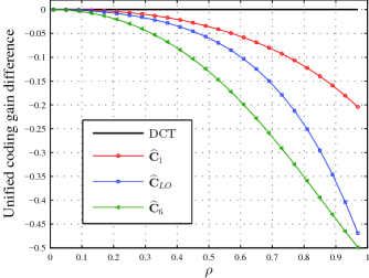
Figure 2 shows the effect of the interpixel correlation ρ𝜌\rho on the performance of the discussed approximate transforms as measured by the unified coding gain difference compared to the exact DCT [73]. The proposed method outperforms the competing methods as its coding gain difference is smaller for any choice of ρ𝜌\rho. For highly correlated data the coding degradation in dB is roughly reduced by half when the proposed approximation 𝐂^1subscript^𝐂1\mathbf{\widehat{C}}_{1} is considered.

Refer to caption
Figure 2: Curves for the coding gain error of 𝐂^1subscript^𝐂1\widehat{\mathbf{C}}_{1}, 𝐂^LOsubscript^𝐂LO\widehat{\mathbf{C}}_{\text{LO}}, and 𝐂^6subscript^𝐂6\widehat{\mathbf{C}}_{6}, relative to the exact DCT, for 0<ρ<10𝜌10<\rho<1.

5 Fast Algorithm and Hardware Realization

5.1 Fast Algorithm

The direct implementation of 𝐓1subscript𝐓1\mathbf{T}_{1} requires 48 additions and 24 bit-shifting operations. However, such computational cost can be significantly reduced by means of sparse matrix factorization [11]. In fact, considering butterfly-based structures as commonly found in decimation-in-frequency algorithms, such as [33, 74, 5], we could derive the following factorization for 𝐓1subscript𝐓1\mathbf{T}_{1}:

𝐓1=𝐃𝐀4𝐀3𝐀2𝐀1,subscript𝐓1𝐃subscript𝐀4subscript𝐀3subscript𝐀2subscript𝐀1\displaystyle\mathbf{T}_{1}=\mathbf{D}\cdot\mathbf{A}_{4}\cdot\mathbf{A}_{3}\cdot\mathbf{A}_{2}\cdot\mathbf{A}_{1},

where:

𝐀1=[1111111111111111],𝐀2=[111111111111],formulae-sequencesubscript𝐀1delimited-[]1missing-subexpressionmissing-subexpressionmissing-subexpressionmissing-subexpressionmissing-subexpressionmissing-subexpression1missing-subexpression1missing-subexpressionmissing-subexpressionmissing-subexpressionmissing-subexpression1missing-subexpressionmissing-subexpressionmissing-subexpression1missing-subexpressionmissing-subexpression1missing-subexpressionmissing-subexpressionmissing-subexpressionmissing-subexpressionmissing-subexpression11missing-subexpressionmissing-subexpressionmissing-subexpressionmissing-subexpressionmissing-subexpressionmissing-subexpression11missing-subexpressionmissing-subexpressionmissing-subexpressionmissing-subexpressionmissing-subexpression1missing-subexpressionmissing-subexpression1missing-subexpressionmissing-subexpressionmissing-subexpression1missing-subexpressionmissing-subexpressionmissing-subexpressionmissing-subexpression1missing-subexpression1missing-subexpressionmissing-subexpressionmissing-subexpressionmissing-subexpressionmissing-subexpressionmissing-subexpression1subscript𝐀2delimited-[]1missing-subexpressionmissing-subexpression1missing-subexpressionmissing-subexpressionmissing-subexpressionmissing-subexpressionmissing-subexpression11missing-subexpressionmissing-subexpressionmissing-subexpressionmissing-subexpressionmissing-subexpressionmissing-subexpression11missing-subexpressionmissing-subexpressionmissing-subexpressionmissing-subexpressionmissing-subexpression1missing-subexpressionmissing-subexpression1missing-subexpressionmissing-subexpressionmissing-subexpressionmissing-subexpressionmissing-subexpressionmissing-subexpressionmissing-subexpressionmissing-subexpression1missing-subexpressionmissing-subexpressionmissing-subexpressionmissing-subexpressionmissing-subexpressionmissing-subexpressionmissing-subexpressionmissing-subexpression1missing-subexpressionmissing-subexpressionmissing-subexpressionmissing-subexpressionmissing-subexpressionmissing-subexpressionmissing-subexpressionmissing-subexpression1missing-subexpressionmissing-subexpressionmissing-subexpressionmissing-subexpressionmissing-subexpressionmissing-subexpressionmissing-subexpressionmissing-subexpression1\displaystyle\mathbf{A}_{1}=\left[\begin{smallmatrix}1&&&&&&&1\\ &1&&&&&1&\\ &&1&&&1&&\\ &&&1&1&&&\\ &&&1&-1&&&\\ &&1&&&-1&&\\ &1&&&&&-1&\\ 1&&&&&&&-1\\ \end{smallmatrix}\right],\quad\mathbf{A}_{2}=\left[\begin{smallmatrix}1&&&1&&&&\\ &1&1&&&&&\\ &1&-1&&&&&\\ 1&&&-1&&&&\\ &&&&1&&&\\ &&&&&1&&\\ &&&&&&1&\\ &&&&&&&1\\ \end{smallmatrix}\right],
𝐀3=[1111111111],𝐀4=[1121112111211211211112],formulae-sequencesubscript𝐀3delimited-[]11missing-subexpressionmissing-subexpressionmissing-subexpressionmissing-subexpressionmissing-subexpressionmissing-subexpression11missing-subexpressionmissing-subexpressionmissing-subexpressionmissing-subexpressionmissing-subexpressionmissing-subexpressionmissing-subexpressionmissing-subexpression1missing-subexpressionmissing-subexpressionmissing-subexpressionmissing-subexpressionmissing-subexpressionmissing-subexpressionmissing-subexpressionmissing-subexpression1missing-subexpressionmissing-subexpressionmissing-subexpressionmissing-subexpressionmissing-subexpressionmissing-subexpressionmissing-subexpressionmissing-subexpression1missing-subexpressionmissing-subexpressionmissing-subexpressionmissing-subexpressionmissing-subexpressionmissing-subexpressionmissing-subexpressionmissing-subexpression1missing-subexpressionmissing-subexpressionmissing-subexpressionmissing-subexpressionmissing-subexpressionmissing-subexpressionmissing-subexpressionmissing-subexpression1missing-subexpressionmissing-subexpressionmissing-subexpressionmissing-subexpressionmissing-subexpressionmissing-subexpressionmissing-subexpressionmissing-subexpression1subscript𝐀4delimited-[]1missing-subexpressionmissing-subexpressionmissing-subexpressionmissing-subexpressionmissing-subexpressionmissing-subexpressionmissing-subexpressionmissing-subexpressionmissing-subexpressionmissing-subexpressionmissing-subexpressionmissing-subexpression1211missing-subexpressionmissing-subexpression12missing-subexpressionmissing-subexpressionmissing-subexpressionmissing-subexpressionmissing-subexpressionmissing-subexpressionmissing-subexpressionmissing-subexpression11missing-subexpression12missing-subexpression1missing-subexpressionmissing-subexpressionmissing-subexpressionmissing-subexpressionmissing-subexpressionmissing-subexpressionmissing-subexpressionmissing-subexpressionmissing-subexpressionmissing-subexpression12missing-subexpression11missing-subexpressionmissing-subexpression21missing-subexpressionmissing-subexpressionmissing-subexpressionmissing-subexpressionmissing-subexpressionmissing-subexpressionmissing-subexpressionmissing-subexpression1112missing-subexpression\displaystyle\mathbf{A}_{3}=\left[\begin{smallmatrix}1&1&&&&&&\\ 1&-1&&&&&&\\ &&1&&&&&\\ &&&1&&&&\\ &&&&1&&&\\ &&&&&1&&\\ &&&&&&1&\\ &&&&&&&1\\ \end{smallmatrix}\right],\quad\mathbf{A}_{4}=\left[\begin{smallmatrix}1&&&&&&&\\ &&&&&\frac{1}{2}&1&1\\ &&1&2&&&&\\ &&&&-1&-1&&\frac{1}{2}\\ &1&&&&&&\\ &&&&\frac{1}{2}&&-1&1\\ &&-2&1&&&&\\ &&&&-1&1&-\frac{1}{2}&\\ \end{smallmatrix}\right],

and 𝐃=diag(1,2,1,2,1,2,1,2)𝐃diag12121212\mathbf{D}=\operatorname{diag}(1,2,1,2,1,2,1,2). Figure 3 shows the signal flow graph (SFG) related to the above factorization. The computational cost of this algorithm is only 24 additions and six multiplications by two. The multiplications by two are extremely simple to be performed, requiring only bit-shifting operations [3]. The fast algorithm proposed requires 50% less additions and 75% less bit-shifting operations when compared to the direct implementation. The computational costs of the considered methods are shown in Table 7. The additive cost of the discussed approximations varies from 14 to 28 additions.

Refer to caption
Figure 3: Signal flow graph of the proposed transform, relating the input data xnsubscript𝑥𝑛x_{n}, n=0,1,,7𝑛017n=0,1,\ldots,7, to its correspondent coefficients X~ksubscript~𝑋𝑘\tilde{X}_{k}, k=0,1,,7𝑘017k=0,1,\ldots,7, where 𝐗~=𝐱𝐓1~𝐗𝐱subscript𝐓1\mathbf{\tilde{X}}=\mathbf{x}\cdot\mathbf{T}_{1}. of 𝐓1subscript𝐓1\mathbf{T}_{1}. Dashed arrows representing multiplication by 11-1.

In general terms, DCT approximations exhibit a trade-off between computational cost and transform performance [61], i.e., less complex matrices effect poor spectral approximations [3]. Departing from this general behavior, the proposed transformation 𝐓𝟏subscript𝐓1\mathbf{T_{1}} has (i) excelling performance measures and (ii) lower or similar arithmetic cost when compared to competing methods, as shown in Tables 5, 6, and 7. Regarding considered performance measures, three transformations are consistenly placed among the five best methods: 𝐓1subscript𝐓1\mathbf{T}_{1}, 𝐓LOsubscript𝐓LO\mathbf{T}_{\text{LO}}, and 𝐓6subscript𝐓6\mathbf{T}_{6}. Thus, we separate them for hardware analysis.

Table 7: Computational cost comparison
Method Multiplications Additions Bit-shifts
DCT [23] 11 29 0
IDCT (HEVC) [72] 0 50 30
𝐓1subscript𝐓1\mathbf{T}_{1} (proposed) 0 24 6
𝐓LOsubscript𝐓LO\mathbf{T}_{\text{LO}} [57] 0 24 2
𝐓SDCTsubscript𝐓SDCT\mathbf{T}_{\text{SDCT}} [51] 0 24 0
𝐓RDCTsubscript𝐓RDCT\mathbf{T}_{\text{RDCT}} [27] 0 22 0
𝐓MRDCTsubscript𝐓MRDCT\mathbf{T}_{\text{MRDCT}} [48] 0 14 0
𝐓BAS-2008asubscript𝐓BAS-2008a\mathbf{T}_{\text{BAS-2008a}} [53] 0 18 2
𝐓BAS-2008bsubscript𝐓BAS-2008b\mathbf{T}_{\text{BAS-2008b}} [52] 0 21 0
𝐓BAS-2009subscript𝐓BAS-2009\mathbf{T}_{\text{BAS-2009}} [54] 0 18 0
𝐓BAS-2011subscript𝐓BAS-2011\mathbf{T}_{\text{BAS-2011}} [55] 0 16 0
𝐓BAS-2013subscript𝐓BAS-2013\mathbf{T}_{\text{BAS-2013}} [56] 0 24 0
𝐓1subscriptsuperscript𝐓1\mathbf{T}^{{}^{\prime}}_{1} [14] 0 18 0
𝐓4subscript𝐓4\mathbf{T}_{4} [14] 0 24 0
𝐓5subscript𝐓5\mathbf{T}_{5} [14] 0 24 4
𝐓6subscript𝐓6\mathbf{T}_{6} [14] 0 24 6

5.2 FPGA Implementation

The proposed design along with 𝐓LOsubscript𝐓LO\mathbf{T}_{\text{LO}} and 𝐓6subscript𝐓6\mathbf{T}_{6} were implemented on an FPGA chip using the Xilinx ML605 board. Considering hardware co-simulation the FPGA realization was tested with 100,000 random 8-point input test vectors. The test vectors were generated from within the MATLAB environment and, using JTAG based hardware co-simulation, routed to the physical FPGA device where each algorithm was realized in the reconfigurable logic fabric. Then the computational results obtained from the FPGA algorithm implementations were routed back to MATLAB memory space. The diagrams for the designs can be seen in Figure 4.

Refer to caption
Refer to caption
Refer to caption
Figure 4: Architectures for (a) 𝐓1subscript𝐓1\mathbf{T}_{1}, (b) 𝐓LOsubscript𝐓LO\mathbf{T}_{\text{LO}}, and (c) 𝐓6subscript𝐓6\mathbf{T}_{6}.

The metrics employed to evaluate the FPGA implementations were: configurable logic blocks (CLB), flip-flop (FF) count, and critical path delay (Tcpdsubscript𝑇cpdT_{\text{cpd}}), in ns. The maximum operating frequency was determined by the critical path delay as Fmaxsubscript𝐹maxF_{\text{max}} = (Tcpd)1superscriptsubscript𝑇cpd1(T_{\text{cpd}})^{-1}, in MHzMHz\mathrm{MHz}. Values were obtained from the Xilinx FPGA synthesis and place-route tools by accessing the xflow.results report file. Using the Xilinx XPower Analyzer, we estimated the static (Qpsubscript𝑄𝑝Q_{p} in WW\mathrm{W}) and dynamic power (Dpsubscript𝐷𝑝D_{p} in mW/MHzmWMHz\mathrm{mW/MHz}) consumption. In addition, we calculated area-time (AT𝐴𝑇AT) and area-time-square (AT2𝐴superscript𝑇2AT^{2}) figures of merit, where area is measured as the CLBs and time as the critical path delay. The values of those metrics for each design are shown in Table 8.

Table 8: Hardware resource consumption and power consumption using Xilinx Virtex-6 XC6VLX240T 1FFG1156 device
Approximation CLB FF
Tcpdsubscript𝑇cpdT_{\text{cpd}}
(nsns\mathrm{ns})
Fmaxsubscript𝐹maxF_{\text{max}}
(MHzMHz\mathrm{MHz})
Dpsubscript𝐷𝑝D_{p}
(mW/GHzmWGHz\mathrm{mW/GHz})
Qpsubscript𝑄𝑝Q_{p}
(WW\mathrm{W})
AT𝐴𝑇AT AT2𝐴superscript𝑇2AT^{2}
𝐓1subscript𝐓1\mathbf{T}_{1} (proposed) 135 408 1.750 571 2.74 3.471 236 413
𝐓LOsubscript𝐓LO\mathbf{T}_{\text{LO}} [57] 114 349 1.900 526 2.82 3.468 217 412
𝐓6subscript𝐓6\mathbf{T}_{6} [14] 125 389 2.100 476 2.57 3.460 262 551

The design linked to the proposed design approximation 𝐓1subscript𝐓1\mathbf{T}_{1} possesses the smallest Tcpdsubscript𝑇cpdT_{\text{cpd}} among the considered methods. Such critical path delay allows for operations at a 8.55%percent8.558.55\% and 19.96%percent19.9619.96\% higher frequency than the designs associated to 𝐓LOsubscript𝐓LO\mathbf{T}_{\text{LO}} and 𝐓6subscript𝐓6\mathbf{T}_{6}, respectively. In terms of area-time and are-time-square measures, the design linked to the approximation 𝐓LOsubscript𝐓LO\mathbf{T}_{\text{LO}} presents the best results, followed by the one associated to 𝐓1subscript𝐓1\mathbf{T}_{1}.

6 Computational Experiments

6.1 Still Image Compression

6.1.1 Experiment Setup and Results

To evaluate the efficiency of the proposed transformation matrix, we performed a JPEG-like image compression experiments as described in [14, 24, 27]. Input images were divided into sub-blocks of size 8×\times8 pixels and submitted to a bidimensional (2-D) transformation, such as the DCT or one of its approximations. Let 𝐀𝐀\mathbf{A} be a sub-block of size 8×\times8. The 2-D approximate transform of 𝐀𝐀\mathbf{A} is an 8×\times8 sub-block 𝐁𝐁\mathbf{B} obtained as follows [14, 46]:

𝐁=𝐂^𝐀𝐂^.𝐁^𝐂𝐀superscript^𝐂top\displaystyle\mathbf{B}=\widehat{\mathbf{C}}\cdot\mathbf{A}\cdot\widehat{\mathbf{C}}^{\top}.

Considering the zig-zag scan pattern as detailed in [75], the initial r𝑟r elements of 𝐁𝐁\mathbf{B} were retained; whereas the remaining (64r)64𝑟(64-r) elements were discarded. Considering 8-bit images, this approach implies that the fixed average bits per pixel equals r/8𝑟8r/8 bits per pixel (bpp). The previous operation results in a matrix 𝐁superscript𝐁\mathbf{B}^{\prime} populated with zeros which is suitable for entropy encoding [16]. Each processed sub-block was submitted to the corresponding 2-D inverse transformation and the image was reconstructed. For orthogonal approximations, the 2-D inverse transform is given by:

𝐀=𝐂^𝐁𝐂^.𝐀superscript^𝐂topsuperscript𝐁^𝐂\displaystyle\mathbf{A}=\widehat{\mathbf{C}}^{\top}\cdot\mathbf{B}^{\prime}\cdot\widehat{\mathbf{C}}.

We considered 44 standardized images obtained from the ‘miscellaneous’ volume from USC-SIPI image bank [76], which include common images such as Lena, Boat, Baboon, and Peppers. Without loss of generality, images were converted to 8-bit grayscale and submitted to the above described procedure. The reconstructed images were compared with the original images and evaluated quantitatively according to popular figures of merit: the mean square error (MSE) [3], the peak signal-to-noise ratio (PSNR) [63] and the structural similarity index (SSIM) [77]. We consider the MSE and PSNR measures because of its good properties and historical usage. However, as discussed in [65], the MSE and PSNR are not the best measures when it comes to predict human perception of image fidelity and quality, for which SSIM has been shown to be a better measure [77, 65].

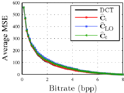
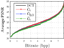
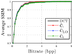
Figure 5 shows the average MSE, PSNR, and SSIM respectively, for the 44 images considering 1<r<641𝑟641<r<64 (bpp from 0 to 8) retained coefficients. The proposed approximation 𝐂^1subscript^𝐂1\mathbf{\widehat{C}}_{1} outperforms 𝐂^LOsubscript^𝐂LO\mathbf{\widehat{C}}_{\text{LO}} and 𝐂^6subscript^𝐂6\mathbf{\widehat{C}}_{6} in terms of MSE and PSNR for any value of r𝑟r. In terms of SSIM, 𝐂^1subscript^𝐂1\mathbf{\widehat{C}}_{1} outperforms 𝐂^6subscript^𝐂6\mathbf{\widehat{C}}_{6} for any value of r𝑟r and 𝐂^LOsubscript^𝐂LO\mathbf{\widehat{C}}_{\text{LO}} for r[7,63]𝑟763r\in[7,63].

Refer to caption
Refer to caption
Refer to caption
Figure 5: Curves for the average of (a) MSE; (b) PSNR; and (c) SSIM corresponding to 44 images.

In order to better visualize previous curves, we adopted the relative difference which is given by [78]:

RD=μ(𝐂)μ(𝐂^)μ(𝐂),𝑅𝐷𝜇𝐂𝜇^𝐂𝜇𝐂\displaystyle RD=\frac{\mu(\mathbf{C})-\mu(\widehat{\mathbf{C}})}{\mu(\mathbf{C})},

where μ(𝐂)𝜇𝐂\mu(\mathbf{C}) and μ(𝐂^)𝜇^𝐂\mu(\widehat{\mathbf{C}}) indicate measurements according to the exact and approximate DCT, respectively; and μ{MSE, PSNR, SSIM}𝜇MSE, PSNR, SSIM\mu\in\{\text{MSE, PSNR, SSIM}\}.

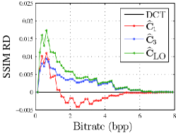
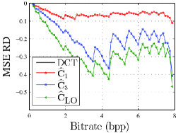
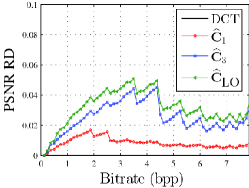
The relative difference for the MSE, PSNR, and SSIM are presented in Figure 6. Figure 6(c) shows that, for 12<r<6012𝑟6012<r<60 (bpp from 1.51.51.5 to 7.57.57.5), 𝐂^1subscript^𝐂1\mathbf{\widehat{C}}_{1} outperforms not only 𝐂^LOsubscript^𝐂LO\mathbf{\widehat{C}}_{\text{LO}} and 𝐂^6subscript^𝐂6\mathbf{\widehat{C}}_{6} but the DCT itself. To the best of our knowledge, this particularly good behavior was never described in literature, where invariably the performance of DCT approximations are routinely bounded by the performance of the exact DCT.
Refer to caption
Refer to caption
Refer to caption
Figure 6: Relative difference curves for (a) MSE; (b) PSNR; and (c) SSIM of 𝐂^1subscript^𝐂1\mathbf{\widehat{C}}_{1}, 𝐂^LOsubscript^𝐂LO\mathbf{\widehat{C}}_{\text{LO}}, and 𝐂^6subscript^𝐂6\mathbf{\widehat{C}}_{6}, relative to the exact DCT.

A qualitative evaluation is provided in Figures 7 and 8, where the reconstructed Lena images [76] for r=3𝑟3r=3 (0.3250.3250.325 bpp) and r=14𝑟14r=14 (1.751.751.75 bpp), respectively, according to the exact DCT, 𝐂^1subscript^𝐂1\mathbf{\widehat{C}}_{1}, 𝐂^LOsubscript^𝐂LO\mathbf{\widehat{C}}_{\text{LO}}, and 𝐂^6subscript^𝐂6\mathbf{\widehat{C}}_{6} are shown. As expected from the results shown in Figure 6(c), for a bitrate lower than 1.51.51.5, the proposed approximate transform matrix is not the one that performs the best (Figure 7), although the results are very similar to the ones furnished by the exact DCT. For a bitrate value larger than 1.51.51.5, Figure 8 demonstrates a situation were the proposed approximation overcomes the other transforms, including the DCT. In both cases, the visual difference between the DCT and the proposed aproximate transform matrix is very small.

Refer to caption
(a) MSE = 119.91, PSNR = 27.34, SSIM = 0.8814.
Refer to caption
(b) MSE = 124.44, PSNR = 27.18, SSIM = 0.8767.
Refer to caption
(c) MSE = 131.08, PSNR = 26.95, SSIM = 0.8781.
Refer to caption
(d) MSE = 129.03, PSNR = 27.02, SSIM = 0.87.63.
Figure 7: Compression of Lena using (a) DCT; (b) 𝐂^1subscript^𝐂1\mathbf{\widehat{C}}_{1}; (c) 𝐂^LOsubscript^𝐂LO\mathbf{\widehat{C}}_{\text{LO}}; and (d) 𝐂^6subscript^𝐂6\mathbf{\widehat{C}}_{6} considering r=3𝑟3r=3 (0.325 bpp).
Refer to caption
(a) MSE = 27.17, PSNR = 33.78, SSIM = 0.9888.
Refer to caption
(b) MSE = 33.48, PSNR = 32.88, SSIM = 0.9893.
Refer to caption
(c) MSE = 40.07, PSNR = 32.10, SSIM = 0.9849.
Refer to caption
(d) MSE = 42.18, PSNR = 31.87, SSIM = 0.9844.
Figure 8: Compression of Lena using (a) DCT; (b) 𝐂^1subscript^𝐂1\mathbf{\widehat{C}}_{1}; (c) 𝐂^LOsubscript^𝐂LO\mathbf{\widehat{C}}_{\text{LO}}; and (d) 𝐂^6subscript^𝐂6\mathbf{\widehat{C}}_{6} considering r=14𝑟14r=14 (1.75).

6.1.2 Discussion

The obtained approximation was capable of outperforming the DCT under the above described conditions. We think that this is relevant, because it directly offers a counter-example to the belief that the coding performance of an approximation is supposed to always be inferior to the DCT. The theoretical background that leads the optimal performance of the DCT is based on assumption that the considered images must follow the Markov-1 processes with high correlation (ρ1𝜌1\rho\to 1). In practice, natural images tend to fit under this assumption, but at lower correlation values the ideal case (ρ1𝜌1\rho\to 1) may not necessarily be met as strongly. For instance, the average correlation of the considered image set was roughly 0.86. This practical deviation from the ideal case (ρ1𝜌1\rho\to 1) may also play a role in explaining our results.

Finding matrix approximation as described in this work is a computational and numerical task. To the best of our knowledge, we cannot identify any methodology that could furnish necessary mathematical tools to design optimal approximations for image compression in an a priori manner, i.e., before search space approaches, optimization problem solving, or numerical simulation. In [3, 5, 61, 25, 79, 80], a large number of methods is listed; all of them aim at good approximations. Although the problem of matrix approximation is quite simple to state, it is also very tricky and offers several non-linearities when combined to a more sophisticate system, such as image compression codecs. Finding low-complexity matrices can be categorized as an integer optimization problem. Thus, navigating in the low-complexity matrix search space might generate non-trivial performance curves, usually leading to discontinuities, which seems to be the case of the proposed approximations matrix 𝐓1subscript𝐓1\mathbf{T}_{1}. The navigation path through the search space is highly dependent on the search method and its objective function. Although approximation methods are very likely to provide reasonable approximations, it is also very hard to tell beforehand whether a given approximation method is capable of furnishing extremely good results capable of outperforming the state of the art. Only after experimentation with the obtained approximations one may know better. In particular, this work advances an optimization setup based on a geometrically intuitive objective function (angle between vectors) that could find good matrices as demonstrated by our a posteriori experiments.

6.2 Video Coding

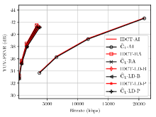
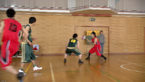
In order to assess the proposed transform 𝐂^1subscript^𝐂1\mathbf{\widehat{C}}_{1} as a tool for video coding, we embedded it into a public available HEVC reference software [81]. The HEVC presents several improvements relative to its predecessors [82] and aims at providing high compression rates [22]. Differently from other standards (cf. Section 1), HEVC employs not only an 8-point integer DCT (IDCT) but also transforms of size 4, 16, and 32 [72]. Such feature effects a series of optimization routines allowing the processing of big smooth or textureless areas [22].

The computational search used in the proposed method proved feasible for the 8-point case. However, as N𝑁N increases, the size of the search space increases very quickly. For the case N=16𝑁16N=16, if considering the low complexity set 𝒫={1,0,1}𝒫101\mathcal{P}=\{-1,0,1\}, we have a search space with 3164.3×107superscript3164.3superscript1073^{16}\approx 4.3\times 10^{7} elements. For this blocklength, The proposed algorithm takes about 6 minutes to find an approximation for a fixed row sequence, considering a machine with the following specifications: 16-core 2.4 GHZ Intel(R) Xeon(R) CPU E5-2630 v3, with 32 GB RAM running Ubuntu 16.04.3 LTS 64-bit. Therefore, since we have N!𝑁N! matrices to be generated, to run the whole algorithm would take approximately 16!×616616!\times 6 minutes. In other words, the computation time would take an extremely large amount of time. Thus, for now, we limited the scope of our computational search to 8-point approximations.

For this reason, aiming to derive large blocklength transforms for HEVC embedding, we submitted the proposed transform matrix 𝐓1subscript𝐓1\mathbf{T}_{1} to the Jridi–Alfalou–Meher (JAM) scalable algorithm [83]. Such method resulted in 16- and 32-point versions of the proposed matrix 𝐓1subscript𝐓1\mathbf{T}_{1} that are suitable for the sought video experiments. Although the JAM algorithm is similar to Chen’s DCT [30], it exploits redundancies allowing concise and high parallelizable hardware implementations [83]. From a low-complexity N/2𝑁2N/2-point transform, the JAM algorithm generates an N×N𝑁𝑁N\times N matrix transformation by combining two instantiations of the smaller one. The larger N𝑁N-point transform is recursively defined by:

𝐓(N)=12𝐌Nper[𝐓(N2)𝐙N2𝐙N2𝐓(N2)]𝐌Nadd,subscript𝐓𝑁12subscriptsuperscript𝐌per𝑁matrixsubscript𝐓𝑁2subscript𝐙𝑁2subscript𝐙𝑁2subscript𝐓𝑁2subscriptsuperscript𝐌add𝑁\displaystyle{\mathbf{T}}_{(N)}=\frac{1}{\sqrt{2}}\mathbf{M}^{\text{per}}_{N}\begin{bmatrix}{\mathbf{T}}_{\left(\frac{N}{2}\right)}&\mathbf{Z}_{\frac{N}{2}}\\ \mathbf{Z}_{\frac{N}{2}}&{\mathbf{T}}_{\left(\frac{N}{2}\right)}\end{bmatrix}\mathbf{M}^{\text{add}}_{N}, (7)

where 𝐙N2subscript𝐙𝑁2\mathbf{Z}_{\frac{N}{2}} is a matrix of order N/2𝑁2N/2 with all zeroed entries. Matrices 𝐌Naddsubscriptsuperscript𝐌add𝑁\mathbf{M}^{\text{add}}_{N} and 𝐌Npersubscriptsuperscript𝐌per𝑁\mathbf{M}^{\text{per}}_{N} are, respectively, obtained according to:

𝐌Nadd=[𝐈N2𝐈¯N2𝐈¯N2𝐈N2]subscriptsuperscript𝐌add𝑁matrixsubscript𝐈𝑁2subscript¯𝐈𝑁2subscript¯𝐈𝑁2subscript𝐈𝑁2\displaystyle\mathbf{M}^{\text{add}}_{N}=\begin{bmatrix}\mathbf{I}_{\frac{N}{2}}&\mathbf{\bar{I}}_{\frac{N}{2}}\\ \mathbf{\bar{I}}_{\frac{N}{2}}&-\mathbf{I}_{\frac{N}{2}}\end{bmatrix}

and

𝐌Nper=[𝐏N1,N2𝐙1,N2𝐙1,N2𝐏N1,N2],subscriptsuperscript𝐌per𝑁matrixsubscript𝐏𝑁1𝑁2subscript𝐙1𝑁2subscript𝐙1𝑁2subscript𝐏𝑁1𝑁2\displaystyle\mathbf{M}^{\text{per}}_{N}=\begin{bmatrix}\mathbf{P}_{N-1,\frac{N}{2}}&\mathbf{Z}_{1,\frac{N}{2}}\\ \mathbf{Z}_{1,\frac{N}{2}}&\mathbf{P}_{N-1,\frac{N}{2}}\end{bmatrix},

where 𝐈N2subscript𝐈𝑁2\mathbf{I}_{\frac{N}{2}} and 𝐈¯N2subscript¯𝐈𝑁2\mathbf{\bar{I}}_{\frac{N}{2}} are, respectively, the identity and counter-identity matrices of order N/2𝑁2N/2 and 𝐏N1,N2subscript𝐏𝑁1𝑁2\mathbf{P}_{N-1,\frac{N}{2}} is an (N1)×(N/2)𝑁1𝑁2(N-1)\times(N/2) matrix whose row vectors are defined by:

𝐏N1,N2(i)={𝐙1,N2,if i=1,3,5,,N1𝐈N2(i/2),if i=0,2,4,,N2.superscriptsubscript𝐏𝑁1𝑁2𝑖casessubscript𝐙1𝑁2if i=1,3,5,,N1superscriptsubscript𝐈𝑁2𝑖2if i=0,2,4,,N2\displaystyle\mathbf{P}_{N-1,\frac{N}{2}}^{(i)}=\begin{cases}\mathbf{Z}_{1,\frac{N}{2}},&\text{if $i=1,3,5,\ldots,N-1$}\\ \mathbf{I}_{\frac{N}{2}}^{(i/2)},&\text{if $i=0,2,4,\ldots,N-2$}.\end{cases}

The scaling factor 1/2121/\sqrt{2} of (7) can be merged into the image/video compression quantization step. Furthermore, (1) can be applied to generate orthogonal versions of larger transforms. The computational cost of the resulting N𝑁N-point transform is given by twice the number of bit-shifting operations of the original N/2𝑁2N/2-point transform; and twice the number of additions plus N𝑁N extra additions. Following the described algorithm, we obtained the 16- and 32-point low complexity transform matrices proposed. More explicitly, we obtained the following 16- and 32-point matrices, respectively:

𝐓(16)=[1111111111111111111111111111111122100122221001222210012222100122211221122112211221122112211221121022220110222201102222011022220111111111111111111111111111111111220110222201102222011022220110221221122112211221122112211221122101222210012222100122221001222210]subscript𝐓16delimited-[]1111111111111111111111111111111122100122221001222210012222100122211221122112211221122112211221121022220110222201102222011022220111111111111111111111111111111111220110222201102222011022220110221221122112211221122112211221122101222210012222100122221001222210\displaystyle\mathbf{T}_{(16)}=\left[\setcounter{MaxMatrixCols}{16}\begin{smallmatrix}1&\phantom{-}1&\phantom{-}1&\phantom{-}1&\phantom{-}1&\phantom{-}1&\phantom{-}1&\phantom{-}1&\phantom{-}1&\phantom{-}1&\phantom{-}1&\phantom{-}1&\phantom{-}1&\phantom{-}1&\phantom{-}1&\phantom{-}1\\ 1&\phantom{-}1&\phantom{-}1&\phantom{-}1&\phantom{-}1&\phantom{-}1&\phantom{-}1&\phantom{-}1&-1&-1&-1&-1&-1&-1&-1&-1\\ 2&\phantom{-}2&\phantom{-}1&\phantom{-}0&\phantom{-}0&-1&-2&-2&-2&-2&-1&\phantom{-}0&\phantom{-}0&\phantom{-}1&\phantom{-}2&\phantom{-}2\\ 2&\phantom{-}2&\phantom{-}1&\phantom{-}0&\phantom{-}0&-1&-2&-2&\phantom{-}2&\phantom{-}2&\phantom{-}1&\phantom{-}0&\phantom{-}0&-1&-2&-2\\ 2&\phantom{-}1&-1&-2&-2&-1&\phantom{-}1&\phantom{-}2&\phantom{-}2&\phantom{-}1&-1&-2&-2&-1&\phantom{-}1&\phantom{-}2\\ 2&\phantom{-}1&-1&-2&-2&-1&\phantom{-}1&\phantom{-}2&-2&-1&\phantom{-}1&\phantom{-}2&\phantom{-}2&\phantom{-}1&-1&-2\\ 1&\phantom{-}0&-2&-2&\phantom{-}2&\phantom{-}2&\phantom{-}0&-1&-1&\phantom{-}0&\phantom{-}2&\phantom{-}2&-2&-2&\phantom{-}0&\phantom{-}1\\ 1&\phantom{-}0&-2&-2&\phantom{-}2&\phantom{-}2&\phantom{-}0&-1&\phantom{-}1&\phantom{-}0&-2&-2&\phantom{-}2&\phantom{-}2&\phantom{-}0&-1\\ 1&-1&-1&\phantom{-}1&\phantom{-}1&-1&-1&\phantom{-}1&\phantom{-}1&-1&-1&\phantom{-}1&\phantom{-}1&-1&-1&\phantom{-}1\\ 1&-1&-1&\phantom{-}1&\phantom{-}1&-1&-1&\phantom{-}1&-1&\phantom{-}1&\phantom{-}1&-1&-1&\phantom{-}1&\phantom{-}1&-1\\ 2&-2&\phantom{-}0&\phantom{-}1&-1&\phantom{-}0&\phantom{-}2&-2&-2&\phantom{-}2&\phantom{-}0&-1&\phantom{-}1&\phantom{-}0&-2&\phantom{-}2\\ 2&-2&\phantom{-}0&\phantom{-}1&-1&\phantom{-}0&\phantom{-}2&-2&\phantom{-}2&-2&\phantom{-}0&\phantom{-}1&-1&\phantom{-}0&\phantom{-}2&-2\\ 1&-2&\phantom{-}2&-1&-1&\phantom{-}2&-2&\phantom{-}1&\phantom{-}1&-2&\phantom{-}2&-1&-1&\phantom{-}2&-2&\phantom{-}1\\ 1&-2&\phantom{-}2&-1&-1&\phantom{-}2&-2&\phantom{-}1&-1&\phantom{-}2&-2&\phantom{-}1&\phantom{-}1&-2&\phantom{-}2&-1\\ 0&-1&\phantom{-}2&-2&\phantom{-}2&-2&\phantom{-}1&\phantom{-}0&\phantom{-}0&\phantom{-}1&-2&\phantom{-}2&-2&\phantom{-}2&-1&\phantom{-}0\\ 0&-1&\phantom{-}2&-2&\phantom{-}2&-2&\phantom{-}1&\phantom{-}0&\phantom{-}0&-1&\phantom{-}2&-2&\phantom{-}2&-2&\phantom{-}1&\phantom{-}0\\ \end{smallmatrix}\right]

and

𝐓(32)=subscript𝐓32absent\displaystyle\mathbf{T}_{(32)}=
[1111111111111111111111111111111111111111111111111111111111111111111111111111111111111111111111111111111111111111111111111111111122100122221001222210012222100122221001222210012222100122221001222210012222100122221001222210012222100122221001222210012222100122211221122112211221122112211221122112211221122112211221122112211221122112211221122112211221122112211221122112211221122112211221121022220110222201102222011022220110222201102222011022220110222201102222011022220110222201102222011022220110222201102222011022220111111111111111111111111111111111111111111111111111111111111111111111111111111111111111111111111111111111111111111111111111111111220110222201102222011022220110222201102222011022220110222201102222011022220110222201102222011022220110222201102222011022220110221221122112211221122112211221122112211221122112211221122112211221122112211221122112211221122112211221122112211221122112211221122101222210012222100122221001222210012222100122221001222210012222100122221001222210012222100122221001222210012222100122221001222210].delimited-[]1111111111111111111111111111111111111111111111111111111111111111111111111111111111111111111111111111111111111111111111111111111122100122221001222210012222100122221001222210012222100122221001222210012222100122221001222210012222100122221001222210012222100122211221122112211221122112211221122112211221122112211221122112211221122112211221122112211221122112211221122112211221122112211221121022220110222201102222011022220110222201102222011022220110222201102222011022220110222201102222011022220110222201102222011022220111111111111111111111111111111111111111111111111111111111111111111111111111111111111111111111111111111111111111111111111111111111220110222201102222011022220110222201102222011022220110222201102222011022220110222201102222011022220110222201102222011022220110221221122112211221122112211221122112211221122112211221122112211221122112211221122112211221122112211221122112211221122112211221122101222210012222100122221001222210012222100122221001222210012222100122221001222210012222100122221001222210012222100122221001222210\displaystyle\tiny\left[\setcounter{MaxMatrixCols}{32}\begin{smallmatrix}1&\phantom{-}1&\phantom{-}1&\phantom{-}1&\phantom{-}1&\phantom{-}1&\phantom{-}1&\phantom{-}1&\phantom{-}1&\phantom{-}1&\phantom{-}1&\phantom{-}1&\phantom{-}1&\phantom{-}1&\phantom{-}1&\phantom{-}1&\phantom{-}1&\phantom{-}1&\phantom{-}1&\phantom{-}1&\phantom{-}1&\phantom{-}1&\phantom{-}1&\phantom{-}1&\phantom{-}1&\phantom{-}1&\phantom{-}1&\phantom{-}1&\phantom{-}1&\phantom{-}1&\phantom{-}1&\phantom{-}1\\ 1&\phantom{-}1&\phantom{-}1&\phantom{-}1&\phantom{-}1&\phantom{-}1&\phantom{-}1&\phantom{-}1&\phantom{-}1&\phantom{-}1&\phantom{-}1&\phantom{-}1&\phantom{-}1&\phantom{-}1&\phantom{-}1&\phantom{-}1&-1&-1&-1&-1&-1&-1&-1&-1&-1&-1&-1&-1&-1&-1&-1&-1\\ 1&\phantom{-}1&\phantom{-}1&\phantom{-}1&\phantom{-}1&\phantom{-}1&\phantom{-}1&\phantom{-}1&-1&-1&-1&-1&-1&-1&-1&-1&-1&-1&-1&-1&-1&-1&-1&-1&\phantom{-}1&\phantom{-}1&\phantom{-}1&\phantom{-}1&\phantom{-}1&\phantom{-}1&\phantom{-}1&\phantom{-}1\\ 1&\phantom{-}1&\phantom{-}1&\phantom{-}1&\phantom{-}1&\phantom{-}1&\phantom{-}1&\phantom{-}1&-1&-1&-1&-1&-1&-1&-1&-1&\phantom{-}1&\phantom{-}1&\phantom{-}1&\phantom{-}1&\phantom{-}1&\phantom{-}1&\phantom{-}1&\phantom{-}1&-1&-1&-1&-1&-1&-1&-1&-1\\ 2&\phantom{-}2&\phantom{-}1&\phantom{-}0&\phantom{-}0&-1&-2&-2&-2&-2&-1&\phantom{-}0&\phantom{-}0&\phantom{-}1&\phantom{-}2&\phantom{-}2&\phantom{-}2&\phantom{-}2&\phantom{-}1&\phantom{-}0&\phantom{-}0&-1&-2&-2&-2&-2&-1&\phantom{-}0&\phantom{-}0&\phantom{-}1&\phantom{-}2&\phantom{-}2\\ 2&\phantom{-}2&\phantom{-}1&\phantom{-}0&\phantom{-}0&-1&-2&-2&-2&-2&-1&\phantom{-}0&\phantom{-}0&\phantom{-}1&\phantom{-}2&\phantom{-}2&-2&-2&-1&\phantom{-}0&\phantom{-}0&\phantom{-}1&\phantom{-}2&\phantom{-}2&\phantom{-}2&\phantom{-}2&\phantom{-}1&\phantom{-}0&\phantom{-}0&-1&-2&-2\\ 2&\phantom{-}2&\phantom{-}1&\phantom{-}0&\phantom{-}0&-1&-2&-2&\phantom{-}2&\phantom{-}2&\phantom{-}1&\phantom{-}0&\phantom{-}0&-1&-2&-2&-2&-2&-1&\phantom{-}0&\phantom{-}0&\phantom{-}1&\phantom{-}2&\phantom{-}2&-2&-2&-1&\phantom{-}0&\phantom{-}0&\phantom{-}1&\phantom{-}2&\phantom{-}2\\ 2&\phantom{-}2&\phantom{-}1&\phantom{-}0&\phantom{-}0&-1&-2&-2&\phantom{-}2&\phantom{-}2&\phantom{-}1&\phantom{-}0&\phantom{-}0&-1&-2&-2&\phantom{-}2&\phantom{-}2&\phantom{-}1&\phantom{-}0&\phantom{-}0&-1&-2&-2&\phantom{-}2&\phantom{-}2&\phantom{-}1&\phantom{-}0&\phantom{-}0&-1&-2&-2\\ 2&\phantom{-}1&-1&-2&-2&-1&\phantom{-}1&\phantom{-}2&\phantom{-}2&\phantom{-}1&-1&-2&-2&-1&\phantom{-}1&\phantom{-}2&\phantom{-}2&\phantom{-}1&-1&-2&-2&-1&\phantom{-}1&\phantom{-}2&\phantom{-}2&\phantom{-}1&-1&-2&-2&-1&\phantom{-}1&\phantom{-}2\\ 2&\phantom{-}1&-1&-2&-2&-1&\phantom{-}1&\phantom{-}2&\phantom{-}2&\phantom{-}1&-1&-2&-2&-1&\phantom{-}1&\phantom{-}2&-2&-1&\phantom{-}1&\phantom{-}2&\phantom{-}2&\phantom{-}1&-1&-2&-2&-1&\phantom{-}1&\phantom{-}2&\phantom{-}2&\phantom{-}1&-1&-2\\ 2&\phantom{-}1&-1&-2&-2&-1&\phantom{-}1&\phantom{-}2&-2&-1&\phantom{-}1&\phantom{-}2&\phantom{-}2&\phantom{-}1&-1&-2&-2&-1&\phantom{-}1&\phantom{-}2&\phantom{-}2&\phantom{-}1&-1&-2&\phantom{-}2&\phantom{-}1&-1&-2&-2&-1&\phantom{-}1&\phantom{-}2\\ 2&\phantom{-}1&-1&-2&-2&-1&\phantom{-}1&\phantom{-}2&-2&-1&\phantom{-}1&\phantom{-}2&\phantom{-}2&\phantom{-}1&-1&-2&\phantom{-}2&\phantom{-}1&-1&-2&-2&-1&\phantom{-}1&\phantom{-}2&-2&-1&\phantom{-}1&\phantom{-}2&\phantom{-}2&\phantom{-}1&-1&-2\\ 1&\phantom{-}0&-2&-2&\phantom{-}2&\phantom{-}2&\phantom{-}0&-1&-1&\phantom{-}0&\phantom{-}2&\phantom{-}2&-2&-2&\phantom{-}0&\phantom{-}1&\phantom{-}1&\phantom{-}0&-2&-2&\phantom{-}2&\phantom{-}2&\phantom{-}0&-1&-1&\phantom{-}0&\phantom{-}2&\phantom{-}2&-2&-2&\phantom{-}0&\phantom{-}1\\ 1&\phantom{-}0&-2&-2&\phantom{-}2&\phantom{-}2&\phantom{-}0&-1&-1&\phantom{-}0&\phantom{-}2&\phantom{-}2&-2&-2&\phantom{-}0&\phantom{-}1&-1&\phantom{-}0&\phantom{-}2&\phantom{-}2&-2&-2&\phantom{-}0&\phantom{-}1&\phantom{-}1&\phantom{-}0&-2&-2&\phantom{-}2&\phantom{-}2&\phantom{-}0&-1\\ 1&\phantom{-}0&-2&-2&\phantom{-}2&\phantom{-}2&\phantom{-}0&-1&\phantom{-}1&\phantom{-}0&-2&-2&\phantom{-}2&\phantom{-}2&\phantom{-}0&-1&-1&\phantom{-}0&\phantom{-}2&\phantom{-}2&-2&-2&\phantom{-}0&\phantom{-}1&-1&\phantom{-}0&\phantom{-}2&\phantom{-}2&-2&-2&\phantom{-}0&\phantom{-}1\\ 1&\phantom{-}0&-2&-2&\phantom{-}2&\phantom{-}2&\phantom{-}0&-1&\phantom{-}1&\phantom{-}0&-2&-2&\phantom{-}2&\phantom{-}2&\phantom{-}0&-1&\phantom{-}1&\phantom{-}0&-2&-2&\phantom{-}2&\phantom{-}2&\phantom{-}0&-1&\phantom{-}1&\phantom{-}0&-2&-2&\phantom{-}2&\phantom{-}2&\phantom{-}0&-1\\ 1&-1&-1&\phantom{-}1&\phantom{-}1&-1&-1&\phantom{-}1&\phantom{-}1&-1&-1&\phantom{-}1&\phantom{-}1&-1&-1&\phantom{-}1&\phantom{-}1&-1&-1&\phantom{-}1&\phantom{-}1&-1&-1&\phantom{-}1&\phantom{-}1&-1&-1&\phantom{-}1&\phantom{-}1&-1&-1&\phantom{-}1\\ 1&-1&-1&\phantom{-}1&\phantom{-}1&-1&-1&\phantom{-}1&\phantom{-}1&-1&-1&\phantom{-}1&\phantom{-}1&-1&-1&\phantom{-}1&-1&\phantom{-}1&\phantom{-}1&-1&-1&\phantom{-}1&\phantom{-}1&-1&-1&\phantom{-}1&\phantom{-}1&-1&-1&\phantom{-}1&\phantom{-}1&-1\\ 1&-1&-1&\phantom{-}1&\phantom{-}1&-1&-1&\phantom{-}1&-1&\phantom{-}1&\phantom{-}1&-1&-1&\phantom{-}1&\phantom{-}1&-1&-1&\phantom{-}1&\phantom{-}1&-1&-1&\phantom{-}1&\phantom{-}1&-1&\phantom{-}1&-1&-1&\phantom{-}1&\phantom{-}1&-1&-1&\phantom{-}1\\ 1&-1&-1&\phantom{-}1&\phantom{-}1&-1&-1&\phantom{-}1&-1&\phantom{-}1&\phantom{-}1&-1&-1&\phantom{-}1&\phantom{-}1&-1&\phantom{-}1&-1&-1&\phantom{-}1&\phantom{-}1&-1&-1&\phantom{-}1&-1&\phantom{-}1&\phantom{-}1&-1&-1&\phantom{-}1&\phantom{-}1&-1\\ 2&-2&\phantom{-}0&\phantom{-}1&-1&\phantom{-}0&\phantom{-}2&-2&-2&\phantom{-}2&\phantom{-}0&-1&\phantom{-}1&\phantom{-}0&-2&\phantom{-}2&\phantom{-}2&-2&\phantom{-}0&\phantom{-}1&-1&\phantom{-}0&\phantom{-}2&-2&-2&\phantom{-}2&\phantom{-}0&-1&\phantom{-}1&\phantom{-}0&-2&\phantom{-}2\\ 2&-2&\phantom{-}0&\phantom{-}1&-1&\phantom{-}0&\phantom{-}2&-2&-2&\phantom{-}2&\phantom{-}0&-1&\phantom{-}1&\phantom{-}0&-2&\phantom{-}2&-2&\phantom{-}2&\phantom{-}0&-1&\phantom{-}1&\phantom{-}0&-2&\phantom{-}2&\phantom{-}2&-2&\phantom{-}0&\phantom{-}1&-1&\phantom{-}0&\phantom{-}2&-2\\ 2&-2&\phantom{-}0&\phantom{-}1&-1&\phantom{-}0&\phantom{-}2&-2&\phantom{-}2&-2&\phantom{-}0&\phantom{-}1&-1&\phantom{-}0&\phantom{-}2&-2&-2&\phantom{-}2&\phantom{-}0&-1&\phantom{-}1&\phantom{-}0&-2&\phantom{-}2&-2&\phantom{-}2&\phantom{-}0&-1&\phantom{-}1&\phantom{-}0&-2&\phantom{-}2\\ 2&-2&\phantom{-}0&\phantom{-}1&-1&\phantom{-}0&\phantom{-}2&-2&\phantom{-}2&-2&\phantom{-}0&\phantom{-}1&-1&\phantom{-}0&\phantom{-}2&-2&\phantom{-}2&-2&\phantom{-}0&\phantom{-}1&-1&\phantom{-}0&\phantom{-}2&-2&\phantom{-}2&-2&\phantom{-}0&\phantom{-}1&-1&\phantom{-}0&\phantom{-}2&-2\\ 1&-2&\phantom{-}2&-1&-1&\phantom{-}2&-2&\phantom{-}1&\phantom{-}1&-2&\phantom{-}2&-1&-1&\phantom{-}2&-2&\phantom{-}1&\phantom{-}1&-2&\phantom{-}2&-1&-1&\phantom{-}2&-2&\phantom{-}1&\phantom{-}1&-2&\phantom{-}2&-1&-1&\phantom{-}2&-2&\phantom{-}1\\ 1&-2&\phantom{-}2&-1&-1&\phantom{-}2&-2&\phantom{-}1&\phantom{-}1&-2&\phantom{-}2&-1&-1&\phantom{-}2&-2&\phantom{-}1&-1&\phantom{-}2&-2&\phantom{-}1&\phantom{-}1&-2&\phantom{-}2&-1&-1&\phantom{-}2&-2&\phantom{-}1&\phantom{-}1&-2&\phantom{-}2&-1\\ 1&-2&\phantom{-}2&-1&-1&\phantom{-}2&-2&\phantom{-}1&-1&\phantom{-}2&-2&\phantom{-}1&\phantom{-}1&-2&\phantom{-}2&-1&-1&\phantom{-}2&-2&\phantom{-}1&\phantom{-}1&-2&\phantom{-}2&-1&\phantom{-}1&-2&\phantom{-}2&-1&-1&\phantom{-}2&-2&\phantom{-}1\\ 1&-2&\phantom{-}2&-1&-1&\phantom{-}2&-2&\phantom{-}1&-1&\phantom{-}2&-2&\phantom{-}1&\phantom{-}1&-2&\phantom{-}2&-1&\phantom{-}1&-2&\phantom{-}2&-1&-1&\phantom{-}2&-2&\phantom{-}1&-1&\phantom{-}2&-2&\phantom{-}1&\phantom{-}1&-2&\phantom{-}2&-1\\ 0&-1&\phantom{-}2&-2&\phantom{-}2&-2&\phantom{-}1&\phantom{-}0&\phantom{-}0&\phantom{-}1&-2&\phantom{-}2&-2&\phantom{-}2&-1&\phantom{-}0&\phantom{-}0&-1&\phantom{-}2&-2&\phantom{-}2&-2&\phantom{-}1&\phantom{-}0&\phantom{-}0&\phantom{-}1&-2&\phantom{-}2&-2&\phantom{-}2&-1&\phantom{-}0\\ 0&-1&\phantom{-}2&-2&\phantom{-}2&-2&\phantom{-}1&\phantom{-}0&\phantom{-}0&\phantom{-}1&-2&\phantom{-}2&-2&\phantom{-}2&-1&\phantom{-}0&\phantom{-}0&\phantom{-}1&-2&\phantom{-}2&-2&\phantom{-}2&-1&\phantom{-}0&\phantom{-}0&-1&\phantom{-}2&-2&\phantom{-}2&-2&\phantom{-}1&\phantom{-}0\\ 0&-1&\phantom{-}2&-2&\phantom{-}2&-2&\phantom{-}1&\phantom{-}0&\phantom{-}0&-1&\phantom{-}2&-2&\phantom{-}2&-2&\phantom{-}1&\phantom{-}0&\phantom{-}0&\phantom{-}1&-2&\phantom{-}2&-2&\phantom{-}2&-1&\phantom{-}0&\phantom{-}0&\phantom{-}1&-2&\phantom{-}2&-2&\phantom{-}2&-1&\phantom{-}0\\ 0&-1&\phantom{-}2&-2&\phantom{-}2&-2&\phantom{-}1&\phantom{-}0&\phantom{-}0&-1&\phantom{-}2&-2&\phantom{-}2&-2&\phantom{-}1&\phantom{-}0&\phantom{-}0&-1&\phantom{-}2&-2&\phantom{-}2&-2&\phantom{-}1&\phantom{-}0&\phantom{-}0&-1&\phantom{-}2&-2&\phantom{-}2&-2&\phantom{-}1&\phantom{-}0\\ \end{smallmatrix}\right].

The resulting approximations for the above low-complexity matrices can be found from (1) and (2). The diagonal matrices implied by (2) are 𝐃(16)=4[1001]diag(4,9,10,9)[1001]subscript𝐃16tensor-product4delimited-[]1001diag49109delimited-[]1001\mathbf{D}_{(16)}=4\cdot\left[\begin{smallmatrix}1&0\\ 0&1\end{smallmatrix}\right]\otimes\operatorname{diag}(4,9,10,9)\otimes\left[\begin{smallmatrix}1&0\\ 0&1\end{smallmatrix}\right] and 𝐃(32)=2𝐃(16)[1001]subscript𝐃32tensor-product2subscript𝐃16delimited-[]1001\mathbf{D}_{(32)}=2\cdot\mathbf{D}_{(16)}\otimes\left[\begin{smallmatrix}1&0\\ 0&1\end{smallmatrix}\right], respectively, where tensor-product\otimes is the Kronecker product [50].

Figures 9 and 10 display the SFG for the low-complexity transform matrices 𝐓(16)subscript𝐓16\mathbf{T}_{(16)} and 𝐓(32)subscript𝐓32\mathbf{T}_{(32)} derived from 𝐓1subscript𝐓1\mathbf{T}_{1}.

Refer to caption
Figure 9: SFG for the proposed 16-point low complexity transform matrix.
Refer to caption
Figure 10: SFG for the proposed 32-point low complexity transform matrix, where 𝐓(16)subscript𝐓16\mathbf{T}_{(16)} is the 16-point matrix presented in Figure 9.

Table 9 lists the computational costs of the proposed transform for sizes N=8,16,32𝑁81632N=8,16,32 compared to an efficient implementation of the IDCT [84].

Table 9: Computational cost comparison for 8-, 16-, and 32-point transforms embedded in HEVC reference software
N𝑁N IDCT [84] Proposed transform
Additions Bit-shifts Additions Bit-shifts
8 50 30 24 6
16 186 86 64 12
32 682 278 160 24

In our experiments, the original 8-, 16-, and 32-point integer transforms of HEVC were substituted by 𝐂^1subscript^𝐂1\mathbf{\widehat{C}}_{1} and its scaled versions. The original 4-point transform was kept unchanged because it is already a very low-complexity transformation. We encoded the first 100 frames of one video sequence of each A to F class in accordance with the common test conditions (CTC) documentation [85]. Namely we used the 8-bit videos: PeopleOnStreet (2560×\times1600 at 30 fps), BasketballDrive (1920×\times1080 at 50 fps), RaceHorses (832×\times480 at 30 fps), BlowingBubbles (416×\times240 at 50 fps), KristenAndSara (1280×\times720 at 60 fps), and BasketbalDrillText (832×\times480 at 50 fps). As suggested in [83], all the test parameters were set according to the CTC documentation. We tested the proposed transforms in All Intra (AI), Random Access (RA), Low Delay B (LD-B), and Low Delay P (LD-P) configurations, all in the Main profile.

We selected the frame-by-frame MSE and PSNR [72] for each YUV color channel as figures of merit. Then, for all test videos, we computed the rate distortion (RD) curve considering the recommended quantization parameter (QP) values, i.e. 22, 27, 32, and 37 [85]. The resulting RD curves are depicted in Figure 11. We have also measured the Bjøntegaard’s delta PSNR (BD-PSNR) and delta rate (BD-Rate) [86, 87] for the modified HEVC software. These values are summarized in Table 10. We demonstrate that replacing the IDCT by the proposed transform and its scaled versions results in a loss in quality of at most 0.47dB for the AI configuration, which corresponds to an increase of 5.82% in bitrate. Worst performance for the other configurations—RA, LD-B, and LD-P—are found for the KristenAndSara video sequence, where approximately 0.55dB are lost if compared to the original HEVC implementation.
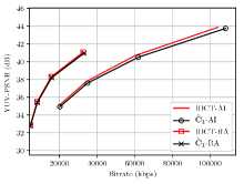
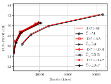
Refer to caption
Refer to caption
Refer to caption
Refer to caption
Refer to caption
Refer to caption
Figure 11: Rate distortion curves of the modified HEVC software for test sequences: (a) PeopleOnStreet, (b) BasketballDrive, (c) RaceHorses, (d) BlowingBubbles, (e) KristenAndSara, and (f) BasketbalDrillText.

Despite the very low computational cost when compared to the IDCT (cf. Table 9), the proposed transform does not introduce significant errors. Figure 12 illustrates the tenth frame of the BasketballDrive video encoded according to the default HEVC IDCT and 𝐂^1subscript^𝐂1\mathbf{\widehat{C}}_{1} and its scaled versions for each coding configuration. The QP was set to 32. Visual degradations are virtually nonperceptible demonstrating real-world applicability of the proposed DCT approximations for high resolution video coding.

Refer to caption
(a) MSE-Y=10.4097MSE-Y10.4097\mbox{MSE-Y}=10.4097, MSE-U=3.5872MSE-U3.5872\mbox{MSE-U}=3.5872, MSE-V=3.3079MSE-V3.3079\mbox{MSE-V}=3.3079, PSNR-Y=37.9564PSNR-Y37.9564\mbox{PSNR-Y}=37.9564, PSNR-U=42.5832PSNR-U42.5832\mbox{PSNR-U}=42.5832, PSNR-V=42.9353PSNR-V42.9353\mbox{PSNR-V}=42.9353
Refer to caption
(b) MSE-Y=10.8159MSE-Y10.8159\mbox{MSE-Y}=10.8159, MSE-U=3.8290MSE-U3.8290\mbox{MSE-U}=3.8290, MSE-V=3.5766MSE-V3.5766\mbox{MSE-V}=3.5766, PSNR-Y=37.7902PSNR-Y37.7902\mbox{PSNR-Y}=37.7902, PSNR-U=42.2999PSNR-U42.2999\mbox{PSNR-U}=42.2999, PSNR-V=42.5961PSNR-V42.5961\mbox{PSNR-V}=42.5961
Refer to caption
(c) MSE-Y=10.1479MSE-Y10.1479\mbox{MSE-Y}=10.1479, MSE-U=3.4765MSE-U3.4765\mbox{MSE-U}=3.4765, MSE-V=3.1724MSE-V3.1724\mbox{MSE-V}=3.1724, PSNR-Y=38.0670PSNR-Y38.0670\mbox{PSNR-Y}=38.0670, PSNR-U=42.7194PSNR-U42.7194\mbox{PSNR-U}=42.7194, PSNR-V=43.1170PSNR-V43.1170\mbox{PSNR-V}=43.1170
Refer to caption
(d) MSE-Y=10.3570MSE-Y10.3570\mbox{MSE-Y}=10.3570, MSE-U=3.6228MSE-U3.6228\mbox{MSE-U}=3.6228, MSE-V=3.3113MSE-V3.3113\mbox{MSE-V}=3.3113, PSNR-Y=37.9785PSNR-Y37.9785\mbox{PSNR-Y}=37.9785, PSNR-U=42.5403PSNR-U42.5403\mbox{PSNR-U}=42.5403, PSNR-V=42.9308PSNR-V42.9308\mbox{PSNR-V}=42.9308
Refer to caption
(e) MSE-Y=14.0693MSE-Y14.0693\mbox{MSE-Y}=14.0693, MSE-U=4.0741MSE-U4.0741\mbox{MSE-U}=4.0741, MSE-V=4.4404MSE-V4.4404\mbox{MSE-V}=4.4404, PSNR-Y=36.6481PSNR-Y36.6481\mbox{PSNR-Y}=36.6481, PSNR-U=42.0304PSNR-U42.0304\mbox{PSNR-U}=42.0304, PSNR-V=41.6566PSNR-V41.6566\mbox{PSNR-V}=41.6566
Refer to caption
(f) MSE-Y=14.5953MSE-Y14.5953\mbox{MSE-Y}=14.5953, MSE-U=4.1377MSE-U4.1377\mbox{MSE-U}=4.1377, MSE-V=4.6053MSE-V4.6053\mbox{MSE-V}=4.6053, PSNR-Y=36.4887PSNR-Y36.4887\mbox{PSNR-Y}=36.4887, PSNR-U=41.9632PSNR-U41.9632\mbox{PSNR-U}=41.9632, PSNR-V=41.4982PSNR-V41.4982\mbox{PSNR-V}=41.4982
Refer to caption
(g) MSE-Y=14.6155MSE-Y14.6155\mbox{MSE-Y}=14.6155, MSE-U=4.1349MSE-U4.1349\mbox{MSE-U}=4.1349, MSE-V=4.5502MSE-V4.5502\mbox{MSE-V}=4.5502, PSNR-Y=36.4827PSNR-Y36.4827\mbox{PSNR-Y}=36.4827, PSNR-U=41.9661PSNR-U41.9661\mbox{PSNR-U}=41.9661, PSNR-V=41.5505PSNR-V41.5505\mbox{PSNR-V}=41.5505
Refer to caption
(h) MSE-Y=15.0761MSE-Y15.0761\mbox{MSE-Y}=15.0761, MSE-U=4.2812MSE-U4.2812\mbox{MSE-U}=4.2812, MSE-V=4.6444MSE-V4.6444\mbox{MSE-V}=4.6444, PSNR-Y=36.3479PSNR-Y36.3479\mbox{PSNR-Y}=36.3479, PSNR-U=41.8151PSNR-U41.8151\mbox{PSNR-U}=41.8151, PSNR-V=41.4615PSNR-V41.4615\mbox{PSNR-V}=41.4615
Figure 12: Compression of the tenth frame of BasketballDrive using (a),(c),(e) the default and (b),(d),(f) the modified versions of the HEVC software for QP=32QP32\mbox{QP}=32, and AI, RA, LD-B, and LD-P coding configurations, respectively.
Table 10: BD-PSNR (dB) and BD-Rate (%) of the modified HEVC reference software for tested video sequences
Video sequence AI RA LD-B LD-P
BD-PSNR BD-Rate BD-PSNR BD-Rate BD-PSNR BD-Rate BD-PSNR BD-Rate
PeopleOnStreet 0.2999 5.53755.5375-5.5375 0.1467 3.43233.4323-3.4323 N/A N/A N/A N/A
BasketballDrive 0.1692 6.10336.1033-6.1033 0.1412 6.18766.1876-6.1876 0.1272 5.27305.2730-5.2730 0.1276 5.24075.2407-5.2407
RaceHorses 0.4714 5.82505.8250-5.8250 0.5521 8.61498.6149-8.6149 0.5460 7.90677.9067-7.9067 0.5344 7.6868limit-from7.6868-7.6868-
BlowingBubbles 0.0839 1.47151.4715-1.4715 0.0821 2.16122.1612-2.1612 0.0806 2.16192.1619-2.1619 0.0813 2.23702.2370-2.2370
KristenAndSara 0.2582 5.04415.0441-5.0441 N/A N/A 0.1230 4.18234.1823-4.1823 0.1118 4.00484.0048-4.0048
BasketballDrillText 0.1036 1.97211.9721-1.9721 0.1372 3.27413.2741-3.2741 0.1748 4.33834.3383-4.3383 0.1646 4.15094.1509-4.1509

7 Conclusion

In this paper, we set up and solved an optimization problem aiming at the proposition of new approximations for the 8-point DCT. The obtained approximations were determined according to a greedy heuristic which minimized the angle between the rows of the approximate and the exact DCT matrices. Constraints of orthogonality and low computational complexity were imposed. One of the obtained approximations outperformed all the considered approximations in literature according to popular performance measures. We also introduced the use of circular statistics for assessing approximate transforms. For the proposed transform 𝐓1subscript𝐓1\mathbf{T}_{1}, a fast algorithm requiring only 24 additions and 6 bit-shifting operations was proposed. The fast algorithm for the proposed method and directly competing approximations were given FPGA realizations. Simulations were made and the hardware resource consumption and power consumption were measured. The maximum operating frequency of the proposed method was 37.4% higher when compared with the well-known Lengwehasatit–Ortega approximation (LO) [57]. In addition, the applicability of the proposed approximation in the context of image compression and video coding was demonstrated. Our experiments also demonstrate that DCT approximations can effectively approximate the DCT behavior, but also—under particular conditions—outperform the DCT itself for image coding. The proposed approximation is fully HEVC-compliant, being capable of video coding with HEVC quality at lower computational costs.

References

  • [1] G. H. Dunteman, Principal components analysis.   Sage, 1989, vol. 69.
  • [2] I. Jolliffe, Principal component analysis.   Wiley Online Library, 2002.
  • [3] V. Britanak, P. Yip, and K. R. Rao, Discrete Cosine and Sine Transforms.   Academic Press, 2007.
  • [4] A. N. Gorban, B. Kgl, D. C. Wunsch, and A. Zinovyev, Principal Manifolds for Data Visualization and Dimension Reduction, 1st ed.   Springer Publishing Company, Incorporated, 2007.
  • [5] K. R. Rao and P. Yip, Discrete Cosine Transform: Algorithms, Advantages, Applications.   San Diego, CA: Academic Press, 1990.
  • [6] H. Chen and B. Zeng, “New transforms tightly bounded by DCT and KLT,” IEEE Signal Processing Letters, vol. 19, no. 6, pp. 344–347, 2012.
  • [7] S. Álvarez-Cortés, N. Amrani, M. Hernández-Cabronero, and J. Serra-Sagristà, “Progressive lossy-to-lossless coding of hyperspectral images through regression wavelet analysis,” International Journal of Remote Sensing, pp. 1–21, 2017.
  • [8] J. Bae and H. Yoo, “Analysis of color transforms for lossless frame memory compression,” International Journal of Applied Engineering Research, vol. 12, no. 24, pp. 15 664–15 667, 2017.
  • [9] D. Thomakos, “Smoothing non-stationary time series using the discrete cosine transform,” Journal of Systems Science and Complexity, vol. 29, no. 2, pp. 382–404, 2016.
  • [10] J. Zeng, G. Cheung, Y.-H. Chao, I. Blanes, J. Serra-Sagristá, and A. Ortega, “Hyperspectral image coding using graph wavelets,” in Proc. IEEE International Conference on Image Processing (ICIP), 2017.
  • [11] R. E. Blahut, Fast algorithms for signal processing.   Cambridge University Press, 2010.
  • [12] N. Ahmed, T. Natarajan, and K. R. Rao, “Discrete cosine transform,” IEEE Transactions on Computers, vol. C-23, no. 1, pp. 90–93, Jan. 1974.
  • [13] R. J. Clarke, “Relation between the Karhunen-Loève and cosine transforms,” IEEE Proceedings F Communications, Radar and Signal Processing, vol. 128, no. 6, pp. 359–360, Nov. 1981.
  • [14] R. J. Cintra, F. M. Bayer, and C. J. Tablada, “Low-complexity 8-point DCT approximations based on integer functions,” Signal Processing, 2014.
  • [15] R. C. Gonzalez and R. E. Woods, Digital image processing, 3rd ed.   Upper Saddle River, NJ, USA: Prentice-Hall, Inc., 2006.
  • [16] G. K. Wallace, “The JPEG still picture compression standard,” IEEE Transactions on Consumer Electronics, vol. 38, no. 1, pp. xviii–xxxiv, February 1992.
  • [17] A. Puri, “Video coding using the H.264/MPEG-4 AVC compression standard,” Signal Processing: Image Communication, vol. 19, 2004.
  • [18] D. J. Le Gall, “The MPEG video compression algorithm,” Signal Processing: Image Communication, vol. 4, no. 2, pp. 129–140, 1992.
  • [19] International Telecommunication Union, “ITU-T recommendation H.261 version 1: Video codec for audiovisual services at p×64𝑝64p\times 64 kbits,” ITU-T, Tech. Rep., 1990.
  • [20] ——, “ITU-T recommendation H.263 version 1: Video coding for low bit rate communication,” ITU-T, Tech. Rep., 1995.
  • [21] A. Luthra, G. J. Sullivan, and T. Wiegand, “Introduction to the special issue on the H.264/AVC video coding standard,” IEEE Transactions on Circuits and Systems for Video Technology, vol. 13, no. 7, pp. 557–559, Jul. 2003.
  • [22] M. T. Pourazad, C. Doutre, M. Azimi, and P. Nasiopoulos, “HEVC: The new gold standard for video compression: How does HEVC compare with H.264/AVC?” IEEE Consumer Electronics Magazine, vol. 1, no. 3, pp. 36–46, Jul. 2012.
  • [23] C. Loeffler, A. Ligtenberg, and G. Moschytz, “Practical fast 1D DCT algorithms with 11 multiplications,” in Proceedings of the International Conference on Acoustics, Speech, and Signal Processing, May 1989, pp. 988–991.
  • [24] U. Sadhvi Potluri, A. Madanayake, R. J. Cintra, F. M. Bayer, S. Kulasekera, and A. Edirisuriya, “Improved 8-point approximate DCT for image and video compression requiring only 14 additions,” Circuits and Systems I: Regular Papers, IEEE Transactions on, vol. 61, no. 6, pp. 1727–1740, 2014.
  • [25] V. A. Coutinho, R. J. Cintra, F. M. Bayer, S. Kulasekera, and A. Madanayake, “A multiplierless pruned DCT-like transformation for image and video compression that requires ten additions only,” Journal of Real-Time Image Processing, pp. 1–9, 2015.
  • [26] F. M. Bayer, R. J. Cintra, A. Edirisuriya, and A. Madanayake, “A digital hardware fast algorithm and FPGA-based prototype for a novel 16-point approximate DCT for image compression applications,” Measurement Science and Technology, vol. 23, no. 8, p. 114010, November 2012.
  • [27] F. M. Bayer and R. J. Cintra, “Image compression via a fast DCT approximation,” IEEE Latin America Transactions, vol. 8, no. 6, pp. 708–713, Dec. 2010.
  • [28] W. Yuan, P. Hao, and C. Xu, “Matrix factorization for fast DCT algorithms,” in IEEE International Conference on Acoustic, Speech, Signal Processing (ICASSP), vol. 3, May 2006, pp. 948–951.
  • [29] Y. Arai, T. Agui, and M. Nakajima, “A fast DCT-SQ scheme for images,” Transactions of the IEICE, vol. E-71, no. 11, pp. 1095–1097, Nov. 1988.
  • [30] W. H. Chen, C. Smith, and S. Fralick, “A fast computational algorithm for the discrete cosine transform,” IEEE Transactions on Communications, vol. 25, no. 9, pp. 1004–1009, September 1977.
  • [31] E. Feig and S. Winograd, “Fast algorithms for the discrete cosine transform,” IEEE Transactions on Signal Processing, vol. 40, no. 9, pp. 2174–2193, September 1992.
  • [32] B. G. Lee, “A new algorithm for computing the discrete cosine transform,” IEEE Transactions on Acoustics, Speech and Signal Processing, vol. ASSP-32, pp. 1243–1245, Dec. 1984.
  • [33] H. S. Hou, “A fast recursive algorithm for computing the discrete cosine transform,” IEEE Transactions on Acoustic, Signal, and Speech Processing, vol. 6, no. 10, pp. 1455–1461, October 1987.
  • [34] M. T. Heideman and C. S. Burrus, Multiplicative complexity, convolution, and the DFT, ser. Signal Processing and Digital Filtering.   Springer-Verlag, 1988.
  • [35] J. Liang and T. D. Tran, “Fast multiplierless approximation of the DCT with the lifting scheme,” IEEE Transactions on Signal Processing, vol. 49, pp. 3032–3044, December 2001.
  • [36] M. Masera, M. Martina, and G. Masera, “Odd type DCT/DST for video coding: Relationships and low-complexity implementations,” 2017.
  • [37] Z. Wang, “Combined DCT and companding for PAPR reduction in OFDM signals.” J. Signal and Information Processing, vol. 2, no. 2, pp. 100–104, 2011.
  • [38] F. S. Snigdha, D. Sengupta, J. Hu, and S. S. Sapatnekar, “Optimal design of JPEG hardware under the approximate computing paradigm,” in Proceedings of the 53rd Annual Design Automation Conference.   ACM, 2016, p. 106.
  • [39] T. Suzuki and M. Ikehara, “Integer DCT based on direct-lifting of DCT-IDCT for lossless-to-lossy image coding,” IEEE Transactions on Image Processing, vol. 19, no. 11, pp. 2958–2965, Nov. 2010.
  • [40] C.-K. Fong and W.-K. Cham, “LLM integer cosine transform and its fast algorithm,” IEEE Transactions on Circuits and Systems for Video Technology, vol. 22, no. 6, pp. 844–854, 2012.
  • [41] K. Choi, S. Lee, and E. S. Jang, “Zero coefficient-aware IDCT algorithm for fast video decoding,” IEEE Transactions on Consumer Electronics, vol. 56, no. 3, 2010.
  • [42] M. Masera, M. Martina, and G. Masera, “Adaptive approximated dct architectures for hevc,” IEEE Transactions on Circuits and Systems for Video Technology, vol. 27, no. 12, pp. 2714–2725, 2017.
  • [43] J.-S. Park, W.-J. Nam, S.-M. Han, and S.-S. Lee, “2-D large inverse transform (16×\times 16, 32×\times 32) for HEVC (high efficiency video coding),” JSTS: Journal of Semiconductor Technology and Science, vol. 12, no. 2, pp. 203–211, 2012.
  • [44] X. Xu, J. Li, X. Huang, M. Dalla Mura, and A. Plaza, “Multiple morphological component analysis based decomposition for remote sensing image classification,” IEEE Transactions on Geoscience and Remote Sensing, vol. 54, no. 5, pp. 3083–3102, 2016.
  • [45] N. J. Higham, “Computing the polar decomposition—with applications,” SIAM Journal on Scientific and Statistical Computing, vol. 7, no. 4, pp. 1160–1174, Oct. 1986.
  • [46] R. J. Cintra and F. M. Bayer, “A DCT approximation for image compression,” IEEE Signal Processing Letters, vol. 18, no. 10, pp. 579–582, Oct. 2011.
  • [47] R. J. Cintra, “An integer approximation method for discrete sinusoidal transforms,” Journal of Circuits, Systems, and Signal Processing, vol. 30, no. 6, pp. 1481–1501, December 2011.
  • [48] F. M. Bayer and R. J. Cintra, “DCT-like transform for image compression requires 14 additions only,” Electronics Letters, vol. 48, no. 15, pp. 919–921, Jul. 2012.
  • [49] N. J. Higham, “Computing real square roots of a real matrix,” Linear Algebra and its Applications, vol. 88–89, pp. 405–430, April 1987.
  • [50] G. A. F. Seber, A Matrix Handbook for Statisticians, ser. Wiley Series in Probability and Mathematical Statistics.   Wiley, 2008.
  • [51] T. I. Haweel, “A new square wave transform based on the DCT,” Signal Processing, vol. 82, pp. 2309–2319, November 2001.
  • [52] S. Bouguezel, M. O. Ahmad, and M. N. S. Swamy, “Low-complexity 8×\times8 transform for image compression,” Electronics Letters, vol. 44, no. 21, pp. 1249–1250, Sep. 2008.
  • [53] ——, “Low-complexity 8×\times8 transform for image compression,” Electronics Letters, vol. 44, no. 21, pp. 1249–1250, 2008.
  • [54] ——, “A fast 8×\times8 transform for image compression,” in 2009 International Conference on Microelectronics (ICM), Dec. 2009, pp. 74–77.
  • [55] ——, “A low-complexity parametric transform for image compression,” in Proceedings of the 2011 IEEE International Symposium on Circuits and Systems, May 2011.
  • [56] ——, “Binary discrete cosine and Hartley transforms,” IEEE Transactions on Circuits and Systems I: Regular Papers, vol. 60, no. 4, pp. 989–1002, April 2013.
  • [57] K. Lengwehasatit and A. Ortega, “Scalable variable complexity approximate forward DCT,” IEEE Transactions on Circuits and Systems for Video Technology, vol. 14, no. 11, pp. 1236–1248, Nov. 2004.
  • [58] R. K. Senapati, U. C. Pati, and K. K. Mahapatra, “A low complexity orthogonal 8×8888\times 8 transform matrix for fast image compression,” Proceeding of the Annual IEEE India Conference (INDICON), Kolkata, India, pp. 1–4, 2010.
  • [59] W. K. Cham, “Development of integer cosine transforms by the principle of dyadic symmetry,” in IEE Proceedings I Communications, Speech and Vision, vol. 136, no. 4, August 1989, pp. 276–282.
  • [60] T. Cormen, C. Leiserson, R. Rivest, and C. Stein, Introduction To Algorithms.   MIT Press, 2001, ch. 16.
  • [61] C. J. Tablada, F. M. Bayer, and R. J. Cintra, “A class of DCT approximations based on the Feig–Winograd algorithm,” Signal Processing, vol. 113, pp. 38–51, 2015.
  • [62] G. Strang, Linear Algebra and Its Applications.   Brooks Cole, Feb. 1988.
  • [63] D. Salomon, G. Motta, and D. Bryant, Data Compression: The Complete Reference, ser. Molecular biology intelligence unit.   Springer, 2007.
  • [64] N. J. Higham and R. S. Schreiber, “Fast polar decomposition of an arbitrary matrix,” Ithaca, NY, USA, Tech. Rep., October 1988.
  • [65] Z. Wang and A. C. Bovik, “Mean squared error: Love it or leave it? A new look at signal fidelity measures,” IEEE Signal Processing Magazine, vol. 26, no. 1, pp. 98–117, Jan. 2009.
  • [66] V. K. Goyal, “Theoretical foundations of transform coding,” IEEE Signal Processing Magazine, vol. 18, no. 5, pp. 9–21, September 2001.
  • [67] J. Katto and Y. Yasuda, “Performance evaluation of subband coding and optimization of its filter coefficients,” Journal of Visual Communication and Image Representation, vol. 2, no. 4, pp. 303–313, December 1991.
  • [68] K. Mardia and P. Jupp, Directional Statistics, ser. Wiley Series in Probability and Statistics.   Wiley, 2009.
  • [69] S. Jammalamadaka and A. Sengupta, Topics in Circular Statistics, ser. Series on multivariate analysis.   World Scientific, 2001.
  • [70] D. S. Watkins, Fundamentals of Matrix Computations, ser. Pure and Applied Mathematics: A Wiley Series of Texts, Monographs and Tracts.   Wiley, 2004.
  • [71] R. P. Mahan, Circular Statistical Methods: Applications in Spatial and Temporal Performance Analysis, ser. Special report.   U.S. Army Research Institute for the Behavioral and Social Sciences, 1991.
  • [72] J.-R. Ohm, G. J. Sullivan, H. Schwarz, T. K. Tan, and T. Wiegand, “Comparison of the coding efficiency of video coding standards - including High Efficiency Video Coding (HEVC),” IEEE Transactions on Circuits and Systems for Video Technology, vol. 22, no. 12, pp. 1669–1684, Dec. 2012.
  • [73] J. Han, Y. Xu, and D. Mukherjee, “A butterfly structured design of the hybrid transform coding scheme,” in Picture Coding Symposium (PCS), 2013.   IEEE, 2013, pp. 17–20.
  • [74] P. Yip and K. Rao, “The decimation-in-frequency algorithms for a family of discrete sine and cosine transforms,” Circuits, Systems and Signal Processing, vol. 7, no. 1, pp. 3–19, 1988.
  • [75] I.-M. Pao and M.-T. Sun, “Approximation of calculations for forward discrete cosine transform,” IEEE Transactions on Circuits and Systems for Video Technology, vol. 8, no. 3, pp. 264–268, Jun. 1998.
  • [76] (2017) USC-SIPI Image Database. University of Southern California. [Online]. Available: http://sipi.usc.edu/database/
  • [77] Z. Wang, A. C. Bovik, H. R. Sheikh, and E. P. Simoncelli, “Image quality assessment: from error visibility to structural similarity,” IEEE Transactions on Image Processing, vol. 13, no. 4, pp. 600–612, Apr. 2004.
  • [78] N. J. Higham, Functions of Matrices: Theory and Computation, ser. SIAM e-books.   Society for Industrial and Applied Mathematics (SIAM, 3600 Market Street, Floor 6, Philadelphia, PA 19104), 2008.
  • [79] R. K. W. Chan and M.-C. Lee, “Multiplierless fast DCT algorithms with minimal approximation errors,” in International Conference on Pattern Recognition, vol. 3.   Los Alamitos, CA, USA: IEEE Computer Society, 2006, pp. 921–925.
  • [80] V. Dimitrov, G. Jullien, and W. Miller, “A new DCT algorithm based on encoding algebraic integers,” in Proceedings of the 1998 IEEE International Conference on Acoustics, Speech and Signal Processing, 1998., vol. 3, May 1998, pp. 1377–1380 vol.3.
  • [81] Joint Collaborative Team on Video Coding (JCT-VC), “HEVC reference software documentation,” 2013, Fraunhofer Heinrich Hertz Institute. [Online]. Available: https://hevc.hhi.fraunhofer.de/
  • [82] G. J. Sullivan, J.-R. Ohm, W.-J. Han, and T. Wiegand, “Overview of the high efficiency video coding (HEVC) standard,” IEEE Trans. Circuits Syst. Video Technol., vol. 22, no. 12, pp. 1649–1668, Dec. 2012.
  • [83] M. Jridi, A. Alfalou, and P. K. Meher, “A generalized algorithm and reconfigurable architecture for efficient and scalable orthogonal approximation of DCT,” IEEE Trans. Circuits Syst. I, vol. 62, no. 2, pp. 449–457, 2015.
  • [84] P. K. Meher, S. Y. Park, B. K. Mohanty, K. S. Lim, and C. Yeo, “Efficient integer DCT architectures for HEVC,” IEEE Transactions on Circuits and Systems for Video Technology, vol. 24, no. 1, pp. 168–178, Jan 2014.
  • [85] F. Bossen, “Common test conditions and software reference configurations,” San Jose, CA, USA, Feb 2013, document JCT-VC L1100.
  • [86] G. Bjøntegaard, “Calculation of average PSNR differences between RD-curves,” in 13th VCEG Meeting, Austin, TX, USA, Apr 2001, document VCEG-M33.
  • [87] P. Hanhart and T. Ebrahimi, “Calculation of average coding efficiency based on subjective quality scores,” Journal of Visual Communication and Image Representation, vol. 25, no. 3, pp. 555 – 564, 2014, qoE in 2D/3D Video Systems.