\epstopdfDeclareGraphicsRule

.tiffpng.pngconvert #1 \OutputFile \AppendGraphicsExtensions.tiff

High Dimensional Model Representation as a Glass Box in Supervised Machine Learning

Caleb Deen Bastian, Herschel Rabitz
Abstract

Prediction and explanation are key objects in supervised machine learning, where predictive models are known as black boxes and explanatory models are known as glass boxes. Explanation provides the necessary and sufficient information to interpret the model output in terms of the model input. It includes assessments of model output dependence on important input variables and measures of input variable importance to model output. High dimensional model representation (HDMR), also known as the generalized functional ANOVA expansion, provides useful insight into the input-output behavior of supervised machine learning models. This article gives applications of HDMR in supervised machine learning. The first application is characterizing information leakage in “big-data” settings. The second application is reduced-order representation of elementary symmetric polynomials. The third application is analysis of variance with correlated variables. The last application is estimation of HDMR from kernel machine and decision tree black box representations. These results suggest HDMR to have broad utility within machine learning as a glass box representation.

1 Introduction

In many areas of science and engineering one is typically interested in using empirical data D to understand an input-output map f𝑓f from some class of systems F𝐹F, often having a large number of input and output variables. We indicate the input space by (X,𝒳)𝑋𝒳(X,\mathscr{X}), the output space by (Y,𝒴)𝑌𝒴(Y,\mathscr{Y}), and the system (model) space as F=YX𝐹superscript𝑌𝑋F=Y^{X}, and put n|X|𝑛𝑋n\equiv|X|\in\mathbb{N} and p|Y|𝑝𝑌p\equiv|Y|\in\mathbb{N} respectively. Suppose D is a collection of iid𝑖𝑖𝑑iid random variables taking values in X×Y𝑋𝑌X\times Y, denoted by D={(xi,yi)}Dsubscript𝑥𝑖subscript𝑦𝑖\textbf{D}=\{(x_{i},y_{i})\}, and regard each (xi,yi)subscript𝑥𝑖subscript𝑦𝑖(x_{i},y_{i}) as a realization from the probability measure ν𝜈\nu.

This setting can be identified to supervised machine learning (Vapnik, 1995), where f𝑓f is a prediction function, F𝐹F is some class of candidate functions, and ν𝜈\nu is the joint probability measure on X×Y𝑋𝑌X\times Y whose independent random realizations form D. The task for supervised machine learning is solving

f=argminfFR(f),superscript𝑓subscriptargmin𝑓𝐹𝑅𝑓f^{*}=\operatorname*{arg\,min}_{f\in F}R(f),

where R𝑅R is a risk functional

R:f1N(x,y)DL(y,f(x)):𝑅maps-to𝑓1𝑁subscript𝑥𝑦D𝐿𝑦𝑓𝑥R:f\mapsto\frac{1}{N}\sum_{(x,y)\in\textbf{D}}L(y,f(x))

with sample size N𝑁N\in\mathbb{N} and where L𝐿L is a loss function, L:X×Y+:𝐿maps-to𝑋𝑌subscriptL:X\times Y\mapsto\mathbb{R}_{+}. The learned fsuperscript𝑓f^{*} is used to assign an element f(x)superscript𝑓𝑥f^{*}(x) of Y𝑌Y to each x𝑥x in X𝑋X. In this article we consider quadratic loss function L(y,f(x))=(yf(x))2𝐿𝑦𝑓𝑥superscript𝑦𝑓𝑥2L(y,f(x))=(y-f(x))^{2}.

1.1 Motivations of representation

The input-output relation f𝑓f can be represented many ways. Black box representation is solely concerned with the task of assigning an element f(x)𝑓𝑥f(x) of Y𝑌Y to each x𝑥x in X𝑋X (prediction) and includes all such functions from X𝑋X into Y𝑌Y. In other words, the particular structure of f𝑓f is irrelevant so long as it is contained in F𝐹F, and notions of input variable importance and dependence of f𝑓f upon the important variables are abstract. General-purpose black box learning algorithms in machine learning include neural networks, kernel machines, and decision tree models. Glass box representation restricts F𝐹F to include only those functions which provide information on variable importance and dependence (explanation). Glass box representation means that F𝐹F is equipped with necessary and sufficient information to interpret the model output in terms of the model input. This information is referred to as interpretative diagnostics and is defined by the variable importance and variable dependence sets I(f)I𝑓\text{I}(f) and P(f)P𝑓\text{P}(f) respectively, each indexed on ({1,,n})Weierstrass-p1𝑛\raisebox{1.79993pt}{\Large$\wp$}(\{1,\dotsc,n\}). Hooker (2007) discusses diagnostics for high-dimensional functions based upon projection operators, and functionals can be further defined to measure variable importance from projections. These ideas are adopted in this article to construct I(f)I𝑓\text{I}(f) and P(f)P𝑓\text{P}(f).

A consideration is managing the sizes of I(f)I𝑓\text{I}(f) and P(f)P𝑓\text{P}(f) as the number of input variables increases, each of size 2nsuperscript2𝑛2^{n}. The exponential growth is known as the curse of dimensionality. For large enough n𝑛n, construction cost outstrips available resources, and feasibility is achieved through simplifying assumptions on F𝐹F or μ𝜇\mu, e.g., stipulating restrictions on model form or distribution. A large body of work supports the ansatz that many high-dimensional systems especially those of a physical (or real-world) nature are accurately, if not exactly, described by representations whose sizes grow polynomially in n𝑛n.

The ansatz is elevated to theorem in a result of Kolmogorov (Lorentz et al., 1996): his superposition theorem, an existence result, establishes that every multivariate continuous function on the unit cube X=[0,1]n𝑋superscript01𝑛X=[0,1]^{n} can be exactly represented using a finite number of univariate continuous functions and the binary operation of addition,

f(x)=i=12n+1ϕi(j=1nψijxj),𝑓𝑥superscriptsubscript𝑖12𝑛1subscriptitalic-ϕ𝑖superscriptsubscript𝑗1𝑛subscript𝜓𝑖𝑗subscript𝑥𝑗f(x)=\sum_{i=1}^{2n+1}\phi_{i}\circ\left(\sum_{j=1}^{n}\psi_{ij}\circ x_{j}\right),

where ϕisubscriptitalic-ϕ𝑖\phi_{i} are ψijsubscript𝜓𝑖𝑗\psi_{ij} are continuous functions. These functions are highly non-smooth, limiting their utility in approximation.

Instead of seeking a representation in terms of univariate functions, suppose a hierarchy of projections into subspaces of increasing dimensions, with the expectation that subspace contributions to output(s) rapidly diminish with increasing dimension. This is the idea behind a mathematical model called high dimensional model representation (HDMR), a finite multivariate representation that efficiently manages the curse of dimensionality and that provides structured information for input-output relationships. When applied to supervised machine learning models, HDMR is a glass box that interprets the model output in terms of the model input.

1.2 Related work

HDMR is discussed as early as Fisher (1921) in ANOVA analysis and has enjoyed extensive application to statistics. When F𝐹F is the collection of symmetric functionals of iid variables HDMR is known as the Hoeffding decomposition, a fundamental object in U-statistics (Hoeffding, 1948). The univariate terms of HDMR are sometimes known as Hajek projections and are extensively used to establish asymptotic normality of various statistics (Hajek, 1968). Global sensitivity analysis (GSA) measures the importance of variables to F𝐹F (Sobol, 2001, 1990; I.M. Sobol, 2004). In GSA applications functional representation of F𝐹F is avoided where instead sensitivity indices are directly estimated. (Rabitz and Alis, 1999) discussed HDMR as a general decomposition of F𝐹F where the input space resides in nsuperscript𝑛\mathbb{R}^{n} or in the n𝑛n-fold product space of arbitrary linear topological function spaces. These ideas have been further developed to F𝐹F for general (non-degenerate) distributions in Hooker (2007), wherein HDMR is known as generalized functional ANOVA, which in turn provisions GSA in terms of structural and correlative sensitivity indices (Li and Rabitz, 2012). Sometimes HDMR is known as the Hoeffding-Sobol decomposition (Chastaing et al., 2012) or Sobol decomposition (Arwade et al., 2010). See Takemura (1983) for references on HDMR’s earlier history.

1.3 Contributions

We discuss HDMR and provide illustrative applications to motivate its utility to supervised machine learning. First, we illustrate that HDMR can diagnose information leakage. This is demonstrated for Pearson goodness-of-fit settings for “big-data” wherein HDMR characterizes estimator efficiency loss and for popular machine learning black boxes wherein HDMR identifies biases. Second, we illustrate that HDMR characterizes the information leakage experienced by partial dependence, another interpretative diagnostic, whenever input variables are correlated. In such settings, HDMR reveals that the interpretative diagnostics functionally depend upon the distribution correlation. Third, we demonstrate that HDMR admits efficient reduced-order representations of high-dimensional models, managing the curse of dimensionality. In particular, we illustrate that the input distribution regulates the efficiency of reduced-order representation in polynomials and demonstrate this effect in a learning setting. Fourth, we demonstrate that HDMR can be applied as a wrapper method for black boxes to provision glass boxes. Fifth, we estimate HDMR of trained kernel machines or ensembles of decision trees.

1.4 Organization

In section 2 we formulate interpretative diagnostics using projection operators and functionals and related quantities. In section 3 we discuss HDMR and provide three examples of applications: (i) to goodness-of-fit in “big-data” settings (subsection 3.1), (ii) high-dimensional modeling (subsection 3.2), and (iii) analysis of variance (subsection 3.3). In section 4 we consider alternative interpretative diagnostics and compare to HDMR for a simple mathematical model having an analytic solution. In section 5 we apply HDMR as a wrapper method for black boxes to convey information on variable importance and dependence, and we consider two machine learning black boxes—kernel machines (subsection 5.1) and decision trees (subsection 5.2)—on analytic and empirical (test dataset) problems. We conclude with a discussion.

2 Preliminaries

In this article we consider the model space to be square-integrable functions F=L2(X,𝒳,μ)𝐹superscript𝐿2𝑋𝒳𝜇F=L^{2}(X,\mathscr{X},\mu). We formulate interpretative diagnostics for the subspaces u{1,,n}𝑢1𝑛u\subseteq\{1,\dotsc,n\} (notationally we use n={1,,n}subscript𝑛1𝑛\mathbb{N}_{n}=\{1,\dotsc,n\} throughout this article) using projection operators and functionals. For every un𝑢subscript𝑛u\subseteq\mathbb{N}_{n} let PusuperscriptP𝑢\textbf{P}^{u} be a projection operator that profiles the dependence of f𝑓f on xusubscript𝑥𝑢x_{u} and put fuPufsubscript𝑓𝑢superscriptP𝑢𝑓f_{u}\equiv\textbf{P}^{u}f; fusubscript𝑓𝑢f_{u} is said to be the variable dependence or projection of f𝑓f on xusubscript𝑥𝑢x_{u}. Let Iu:F+:superscriptI𝑢maps-to𝐹subscript\textbf{I}^{u}:F\mapsto\mathbb{R}_{+} be a functional that measures the importance of fF𝑓𝐹f\in F on xusubscript𝑥𝑢x_{u} and put SuIufsubscript𝑆𝑢superscriptI𝑢𝑓S_{u}\equiv\textbf{I}^{u}f; Susubscript𝑆𝑢S_{u} is said to be a measure of variable importance of f𝑓f on xusubscript𝑥𝑢x_{u}. Using {Iu}superscriptI𝑢\{\textbf{I}^{u}\} and {Pu}superscriptP𝑢\{\textbf{P}^{u}\}, we define respective variable importance and variable dependence sets I(f){Iuf}I𝑓superscriptI𝑢𝑓\text{I}(f)\equiv\{\textbf{I}^{u}f\} and P(f){Puf}P𝑓superscriptP𝑢𝑓\text{P}(f)\equiv\{\textbf{P}^{u}f\} on (n)Weierstrass-psubscript𝑛\raisebox{1.79993pt}{\Large$\wp$}(\mathbb{N}_{n}).

Sometimes total and relative notions of variable importance are necessary. We define the total variable importance of f𝑓f on xisubscript𝑥𝑖x_{i} as TiTifsubscript𝑇𝑖superscriptT𝑖𝑓T_{i}\equiv\textbf{T}^{i}f where TiuiIusuperscriptT𝑖subscript𝑖𝑢superscriptI𝑢\textbf{T}^{i}\equiv\sum_{u\supset i}\textbf{I}^{u}. We define the relative variable importance of f𝑓f on xisubscript𝑥𝑖x_{i} as RiRifsubscript𝑅𝑖superscriptR𝑖𝑓R_{i}\equiv\textbf{R}^{i}f where RifTif/jTjfsuperscriptR𝑖𝑓superscriptT𝑖𝑓subscript𝑗superscriptT𝑗𝑓\textbf{R}^{i}f\equiv\textbf{T}^{i}f/\sum_{j}\textbf{T}^{j}f. Using {Ti}superscriptT𝑖\{\textbf{T}^{i}\} and {Ri}superscriptR𝑖\{\textbf{R}^{i}\} we define total variable importance and relative variable importance sets T(f)={Tif}T𝑓superscriptT𝑖𝑓\text{T}(f)=\{\textbf{T}^{i}f\} and R(f)={Rif}R𝑓superscriptR𝑖𝑓\text{R}(f)=\{\textbf{R}^{i}f\}.

Using I(f)I𝑓\text{I}(f), P(f)P𝑓\text{P}(f), T(f)T𝑓\text{T}(f), and R(f)R𝑓\text{R}(f), we can pose various questions for f𝑓f as super level-sets:

  1. (i)

    which variables are important overall?

    Tϵ(f)={TiT(f):Tiϵ}subscriptTitalic-ϵ𝑓conditional-setsubscript𝑇𝑖T𝑓subscript𝑇𝑖italic-ϵ\text{T}_{\epsilon}(f)=\{T_{i}\in\text{T}(f):T_{i}\geq\epsilon\}
  2. (ii)

    what are the relative importances of the variables?

    Rϵ(f)={RiR(f):Riϵ}.subscriptRitalic-ϵ𝑓conditional-setsubscript𝑅𝑖R𝑓subscript𝑅𝑖italic-ϵ\text{R}_{\epsilon}(f)=\{R_{i}\in\text{R}(f):R_{i}\geq\epsilon\}.
  3. (iii)

    which variables are important individually?

    Iϵ(f)={SuI(f):Suϵ,|u|=1}subscriptIitalic-ϵ𝑓conditional-setsubscript𝑆𝑢I𝑓formulae-sequencesubscript𝑆𝑢italic-ϵ𝑢1\text{I}_{\epsilon}(f)=\{S_{u}\in\text{I}(f):S_{u}\geq\epsilon,|u|=1\}
  4. (iv)

    which variables participate in interactions?

    Xϵ(f)={SuI(f):Suϵ,|u|>1}subscriptXitalic-ϵ𝑓conditional-setsubscript𝑆𝑢I𝑓formulae-sequencesubscript𝑆𝑢italic-ϵ𝑢1\text{X}_{\epsilon}(f)=\{S_{u}\in\text{I}(f):S_{u}\geq\epsilon,|u|>1\}
  5. (v)

    how does the system depend upon the important variables and interactions?

    Pϵ(f)={fuP(f):I(f)Suϵ}subscriptPitalic-ϵ𝑓conditional-setsubscript𝑓𝑢P𝑓contains𝐼𝑓subscript𝑆𝑢italic-ϵ\text{P}_{\epsilon}(f)=\{f_{u}\in\text{P}(f):I(f)\ni S_{u}\geq\epsilon\}
  6. (vi)

    does the system admit a reduced order representation?

    T{1,,n}:ffT=u:|u|Tfu:𝑇1𝑛similar-to-or-equals𝑓superscript𝑓𝑇subscript:𝑢𝑢𝑇subscript𝑓𝑢\exists\,T\in\{1,\dotsc,n\}:\,\,\,f\simeq f^{T}=\sum_{u:|u|\leq T}f_{u}

3 High dimensional model representation

Writing F=L2(X,𝒳,ν)𝐹superscript𝐿2𝑋𝒳𝜈F=L^{2}(X,\mathscr{X},\nu), the HDMR of f(x)F𝑓𝑥𝐹f(x)\in F is the solution to the variational problem

minuf(x)u,u𝒱0i𝒱ii1<i2𝒱i1i2i1<<il𝒱i1il,subscript𝑢𝑓𝑥𝑢𝑢direct-sumsubscript𝒱0subscript𝑖subscript𝒱𝑖subscriptsubscript𝑖1subscript𝑖2subscript𝒱subscript𝑖1subscript𝑖2subscriptsubscript𝑖1subscript𝑖𝑙subscript𝒱subscript𝑖1subscript𝑖𝑙\min_{u}\lVert f(x)-u\rVert,\,\,\,\,\,u\in\mathcal{V}_{0}\oplus\sum_{i}\mathcal{V}_{i}\oplus\sum_{i_{1}<i_{2}}\mathcal{V}_{i_{1}i_{2}}\oplus\dotsc\oplus\sum_{i_{1}<\dotsb<i_{l}}\mathcal{V}_{i_{1}\dotsc i_{l}},

where the norm delimited-∥∥\lVert\cdot\rVert is induced by the inner product as =,1/2delimited-∥∥superscript12\lVert\cdot\rVert=\langle\cdot,\cdot\rangle^{1/2} and the {𝒱uF:|u|l}conditional-setsubscript𝒱𝑢𝐹𝑢𝑙\{\mathcal{V}_{u}\subset F:|u|\leq l\} are subspaces having certain null integral properties. It is uniquely minimized by

u=(𝒫0+i𝒫i+i1<i2𝒫i1i2++i1<<il𝒫i1il)f(x)𝑢subscript𝒫0subscript𝑖subscript𝒫𝑖subscriptsubscript𝑖1subscript𝑖2subscript𝒫subscript𝑖1subscript𝑖2subscriptsubscript𝑖1subscript𝑖𝑙subscript𝒫subscript𝑖1subscript𝑖𝑙𝑓𝑥u=\left(\mathscr{P}_{0}+\sum_{i}\mathscr{P}_{i}+\sum_{i_{1}<i_{2}}\mathscr{P}_{i_{1}i_{2}}+\dotsb+\sum_{i_{1}<\dotsb<i_{l}}\mathscr{P}_{i_{1}\dotsc i_{l}}\right)f(x)

using the collection of non-orthogonal projection operators {𝒫u}subscript𝒫𝑢\{\mathscr{P}_{u}\}. Putting

εl(x)f(x)u=f(x)f0ifi(xi)i1<i2fi1i2(xi1,xi2)i1<<ilfi1il(xi1,,xil),subscript𝜀𝑙𝑥𝑓𝑥𝑢𝑓𝑥subscript𝑓0subscript𝑖subscript𝑓𝑖subscript𝑥𝑖subscriptsubscript𝑖1subscript𝑖2subscript𝑓subscript𝑖1subscript𝑖2subscript𝑥subscript𝑖1subscript𝑥subscript𝑖2subscriptsubscript𝑖1subscript𝑖𝑙subscript𝑓subscript𝑖1subscript𝑖𝑙subscript𝑥subscript𝑖1subscript𝑥subscript𝑖𝑙\varepsilon_{l}(x)\equiv f(x)-u=f(x)-f_{0}-\sum_{i}f_{i}(x_{i})-\sum_{i_{1}<i_{2}}f_{i_{1}i_{2}}(x_{i_{1}},x_{i_{2}})-\dotsb-\sum_{i_{1}<\dotsb<i_{l}}f_{i_{1}\dotsb i_{l}}(x_{i_{1}},\dotsc,x_{i_{l}}),

we express

f(x)u=εl,εl1/2,delimited-∥∥𝑓𝑥𝑢superscriptsubscript𝜀𝑙subscript𝜀𝑙12\lVert f(x)-u\rVert=\langle\varepsilon_{l},\varepsilon_{l}\rangle^{1/2},

which for scalar valued functions is

f(x)u=Xεl2(x)dν(x).delimited-∥∥𝑓𝑥𝑢subscript𝑋superscriptsubscript𝜀𝑙2𝑥differential-d𝜈𝑥\lVert f(x)-u\rVert=\int_{X}\varepsilon_{l}^{2}(x)\mathrm{d}\nu(x).

The HDMR of fF𝑓𝐹f\in F is written as

f(x)=f0+ifi(xi)+i1<i2fi1i2(xi1,xi2)++f1n(x1,,xn),𝑓𝑥subscript𝑓0subscript𝑖subscript𝑓𝑖subscript𝑥𝑖subscriptsubscript𝑖1subscript𝑖2subscript𝑓subscript𝑖1subscript𝑖2subscript𝑥subscript𝑖1subscript𝑥subscript𝑖2subscript𝑓1𝑛subscript𝑥1subscript𝑥𝑛f(x)=f_{0}+\sum_{i}f_{i}(x_{i})+\sum_{i_{1}<i_{2}}f_{i_{1}i_{2}}(x_{i_{1}},x_{i_{2}})+\dotsc+f_{1\dotsc n}(x_{1},\dotsc,x_{n}),

, a sum of 2nsuperscript2𝑛2^{n} component functions (Rabitz and Alis, 1999; Hooker, 2007). Although many additional component functions appear when compared to Kolmogorov’s result, most of these are identically zero or insignificant for many F𝐹F of practical interest: it is often observed

f(x)fT(x)=f0+ifi(xi)+i1<i2fi1i2(xi1,xi2)++i1<<iTfi1iT(xi1,,xiT)𝑓𝑥superscript𝑓𝑇𝑥subscript𝑓0subscript𝑖subscript𝑓𝑖subscript𝑥𝑖subscriptsubscript𝑖1subscript𝑖2subscript𝑓subscript𝑖1subscript𝑖2subscript𝑥subscript𝑖1subscript𝑥subscript𝑖2subscriptsubscript𝑖1subscript𝑖𝑇subscript𝑓subscript𝑖1subscript𝑖𝑇subscript𝑥subscript𝑖1subscript𝑥subscript𝑖𝑇f(x)\backsimeq f^{T}(x)=f_{0}+\sum_{i}f_{i}(x_{i})+\sum_{i_{1}<i_{2}}f_{i_{1}i_{2}}(x_{i_{1}},x_{i_{2}})+\dotsc+\sum_{i_{1}<\dotsc<i_{T}}f_{i_{1}\dotsc i_{T}}(x_{i_{1}},\dotsc,x_{i_{T}})

for Tnmuch-less-than𝑇𝑛T\ll n, i.e. fTsuperscript𝑓𝑇f^{T} is a reduced-order representation of f𝑓f. Whenever T<n𝑇𝑛T<n and f(x)fT(x)similar-to-or-equals𝑓𝑥superscript𝑓𝑇𝑥f(x)\simeq f^{T}(x), we achieve a polynomial-scaling representation in n𝑛n. In most applications T3𝑇3T\leq 3 is sufficient. In general, HDMR is expected to exhibit favorable convergence in T𝑇T whenever the input variables are meaningfully defined in relation to the output variable(s), typically the case with physical systems where input and output variables correspond to observable physical states. Some properties of HDMR:

  1. (i)

    it is unique given μ𝜇\mu

  2. (ii)

    {𝒱u}subscript𝒱𝑢\{\mathcal{V}_{u}\} are hierarchically orthogonal and partition variance, 𝕍ar(f)=u,vov(fu,fv)𝕍ar𝑓subscript𝑢𝑣ovsubscript𝑓𝑢subscript𝑓𝑣\mathbb{V}\text{ar}(f)=\sum_{u,v}\mathbb{C}\text{ov}\left(f_{u},f_{v}\right)

  3. (iii)

    {𝒱u}subscript𝒱𝑢\{\mathcal{V}_{u}\} maximize explained variance, i.e. no other hierarchically-orthogonal functions achieve higher explanatory variance than those belonging to {𝒱u}subscript𝒱𝑢\{\mathcal{V}_{u}\}

  4. (iv)

    the elements of {𝒱u}subscript𝒱𝑢\{\mathcal{V}_{u}\} can be attained through the action of projection operators {𝒫u}subscript𝒫𝑢\{\mathscr{P}_{u}\} such that fu(xu)𝒫uf(x)subscript𝑓𝑢subscript𝑥𝑢subscript𝒫𝑢𝑓𝑥f_{u}(x_{u})\equiv\mathscr{P}_{u}f(x), i.e. the component functions are L2superscript𝐿2L^{2} projections of f(x)𝑓𝑥f(x)

  5. (v)

    all HDMR’s converge at the same order: if fT(x)superscript𝑓𝑇𝑥f^{T}(x) converges for μ𝜇\mu with error 𝒪(ϵ)𝒪italic-ϵ\mathcal{O}(\epsilon), then fT(x)superscript𝑓𝑇𝑥f^{T}(x) converges for μsuperscript𝜇\mu^{\prime} with error 𝒪(ϵ)𝒪italic-ϵ\mathcal{O}(\epsilon), although the constant can be substantially different

  6. (vi)

    for a set of functions {fi(x)}superscript𝑓𝑖𝑥\{f^{i}(x)\} obeying linear-superposition conservation laws, the corresponding HDMR’s obey such for every T𝑇T.

The notion of hierarchical-orthogonality guarantees the existence and uniqueness of the decomposition such that 𝕍ar(f)=u,vov(fu,fv)𝕍ar𝑓subscript𝑢𝑣ovsubscript𝑓𝑢subscript𝑓𝑣\mathbb{V}\text{ar}(f)=\sum_{u,v}\mathbb{C}\text{ov}(f_{u},f_{v}) (Hooker, 2007). Note that hierarchical-orthogonality is a generalization of mutual orthogonality where functions are orthogonal only to functions on nested subspaces. For example, for μ123μ1μ2μ3subscript𝜇123subscript𝜇1subscript𝜇2subscript𝜇3\mu_{123}\neq\mu_{1}\mu_{2}\mu_{3}, hierarchical-orthogonality implies f12,f1=f12,f2=0subscript𝑓12subscript𝑓1subscript𝑓12subscript𝑓20\langle f_{12},f_{1}\rangle=\langle f_{12},f_{2}\rangle=0 but neither implies f1,f2=0subscript𝑓1subscript𝑓20\langle f_{1},f_{2}\rangle=0 nor f12,f3=0subscript𝑓12subscript𝑓30\langle f_{12},f_{3}\rangle=0.

Given the variance decomposition, sensitivity indices can be defined in terms of normalized variances and covariances. This is known as structural and correlative sensitivity analysis (SCSA) (Li and Rabitz, 2012), where SCSA defines structural, correlative, and overall sensitivity indices (𝕊ua,𝕊ub,𝕊u)superscriptsubscript𝕊𝑢asuperscriptsubscript𝕊𝑢bsubscript𝕊𝑢(\mathbb{S}_{u}^{\text{a}},\mathbb{S}_{u}^{\text{b}},\mathbb{S}_{u}) for each component function un𝑢subscript𝑛u\subseteq\mathbb{N}_{n},

𝕊uasuperscriptsubscript𝕊𝑢a\displaystyle\mathbb{S}_{u}^{\text{a}} 1𝕍ar(f)𝕍ar(fu)absent1𝕍ar𝑓𝕍arsubscript𝑓𝑢\displaystyle\equiv\frac{1}{\mathbb{V}\text{ar}(f)}\mathbb{V}\text{ar}(f_{u})
𝕊ubsuperscriptsubscript𝕊𝑢b\displaystyle\mathbb{S}_{u}^{\text{b}} 1𝕍ar(f)v:vuov(fu,fv)absent1𝕍ar𝑓subscript:𝑣𝑣𝑢ovsubscript𝑓𝑢subscript𝑓𝑣\displaystyle\equiv\frac{1}{\mathbb{V}\text{ar}(f)}\sum_{v:v\neq u}\mathbb{C}\text{ov}(f_{u},f_{v})
𝕊usubscript𝕊𝑢\displaystyle\mathbb{S}_{u} 𝕊ua+𝕊ub,absentsuperscriptsubscript𝕊𝑢asuperscriptsubscript𝕊𝑢b\displaystyle\equiv\mathbb{S}_{u}^{\text{a}}+\mathbb{S}_{u}^{\text{b}},

and these satisfy

u𝕊u=1.subscript𝑢subscript𝕊𝑢1\sum_{u}\mathbb{S}_{u}=1.

Note that when μiμi𝜇subscriptproduct𝑖subscript𝜇𝑖\mu\neq\prod_{i}\mu_{i}, the projections fu=𝒫ufsubscript𝑓𝑢subscript𝒫𝑢𝑓f_{u}=\mathscr{P}_{u}f are hierarchically-orthogonal with u𝕊ua<1subscript𝑢superscriptsubscript𝕊𝑢a1\sum_{u}\mathbb{S}_{u}^{\text{a}}<1 and u(𝕊ua+𝕊ub)=1subscript𝑢superscriptsubscript𝕊𝑢asubscriptsuperscript𝕊b𝑢1\sum_{u}(\mathbb{S}_{u}^{\text{a}}+\mathbb{S}^{\text{b}}_{u})=1.

When the input variables are independent, μ=iμi𝜇subscriptproduct𝑖subscript𝜇𝑖\mu=\prod_{i}\mu_{i}, the component functions are mutually orthogonal and can be recursively constructed,

fi1il(xi1,,xil)subscript𝑓subscript𝑖1subscript𝑖𝑙subscript𝑥subscript𝑖1subscript𝑥subscript𝑖𝑙absent\displaystyle f_{i_{1}\dotsc i_{l}}(x_{i_{1}},\dotsc,x_{i_{l}})\equiv Mi1ilf(x)j1<<jl1{i1,,il}fj1jl1(xj1,,xjl1)superscriptMsubscript𝑖1subscript𝑖𝑙𝑓𝑥subscriptsubscript𝑗1subscript𝑗𝑙1subscript𝑖1subscript𝑖𝑙subscript𝑓subscript𝑗1subscript𝑗𝑙1subscript𝑥subscript𝑗1subscript𝑥subscript𝑗𝑙1\displaystyle\,\textbf{M}^{i_{1}\dotsc i_{l}}f(x)-\sum_{j_{1}<\dotsb<j_{l-1}\subset\{i_{1},\dotsc,i_{l}\}}f_{j_{1}\dotsc j_{l-1}}(x_{j_{1}},\dotsc,x_{j_{l-1}})
j1<<jl2{i1,,il}fj1jl2(xj1,,xjl2)subscriptsubscript𝑗1subscript𝑗𝑙2subscript𝑖1subscript𝑖𝑙subscript𝑓subscript𝑗1subscript𝑗𝑙2subscript𝑥subscript𝑗1subscript𝑥subscript𝑗𝑙2\displaystyle-\sum_{j_{1}<\dotsb<j_{l-2}\subset\{i_{1},\dotsc,i_{l}\}}f_{j_{1}\dotsc j_{l-2}}(x_{j_{1}},\dotsc,x_{j_{l-2}})-\dotsb
j{i1,,il}fj(xj)f0subscript𝑗subscript𝑖1subscript𝑖𝑙subscript𝑓𝑗subscript𝑥𝑗subscript𝑓0\displaystyle-\sum_{j\subset\{i_{1},\dotsc,i_{l}\}}f_{j}(x_{j})-f_{0} (1)

where Mi1ilf(x)Xi1ilf(x)j{i1,,il}dμj(xj)superscriptMsubscript𝑖1subscript𝑖𝑙𝑓𝑥subscriptsubscript𝑋subscript𝑖1subscript𝑖𝑙𝑓𝑥subscriptproduct𝑗subscript𝑖1subscript𝑖𝑙dsubscript𝜇𝑗subscript𝑥𝑗\textbf{M}^{i_{1}\dotsc i_{l}}f(x)\equiv\int_{X_{-i_{1}\dotsc i_{l}}}f(x)\prod_{j\notin\{i_{1},\dotsc,i_{l}\}}\mathrm{d}\mu_{j}(x_{j}) (note that (3) does not hold for correlated μ𝜇\mu). Because of the mutual orthogonality of the component functions, we have ov(fu,fv)=0ovsubscript𝑓𝑢subscript𝑓𝑣0\mathbb{C}\text{ov}(f_{u},f_{v})=0 for uv𝑢𝑣u\neq v such that u𝕊ua=1subscript𝑢subscriptsuperscript𝕊a𝑢1\sum_{u}\mathbb{S}^{\text{a}}_{u}=1. This is known as global sensitivity analysis (GSA) Sobol (1990).

In regard to the projection operators {Pu}superscriptP𝑢\{\textbf{P}^{u}\} and functionals {Iu}superscriptI𝑢\{\textbf{I}^{u}\} of interpretative diagnostics, we put for every u𝑢u

PHDMRuf(x)𝒫uf(x)=fuHDMR(xu)subscriptsuperscriptP𝑢HDMR𝑓𝑥subscript𝒫𝑢𝑓𝑥subscriptsuperscript𝑓HDMR𝑢subscript𝑥𝑢{\color[rgb]{0,0,0}\textbf{P}^{u}_{\text{HDMR}}}f(x)\equiv\mathscr{P}_{u}f(x)={\color[rgb]{0,0,0}f^{\text{HDMR}}_{u}(x_{u})}

and

IHDMRuf(x)(𝕊ua,𝕊ub,𝕊u).subscriptsuperscriptI𝑢HDMR𝑓𝑥subscriptsuperscript𝕊a𝑢subscriptsuperscript𝕊b𝑢subscript𝕊𝑢{\color[rgb]{0,0,0}\textbf{I}^{u}_{\text{HDMR}}}f(x)\equiv(\mathbb{S}^{\text{a}}_{u},\mathbb{S}^{\text{b}}_{u},\mathbb{S}_{u}).

We provide three examples of HDMR in machine learning.

3.1 Eliminating information leakage in “big-data” settings

Consider an independency of iid random variables D={Xi}Dsubscript𝑋𝑖\textbf{D}=\{X_{i}\} with distribution μ𝜇\mu on X𝑋X. Suppose (X,𝒳)𝑋𝒳(X,\mathscr{X}) is discrete and that D is represented as an infinite double-array [Xnj]delimited-[]subscript𝑋𝑛𝑗[X_{nj}] of real-valued random variables (that is, for each n𝑛n\in\mathbb{N} there is a knsubscript𝑘𝑛k_{n}\in\mathbb{N} such that Xnj=0subscript𝑋𝑛𝑗0X_{nj}=0 for all j>kn𝑗subscript𝑘𝑛j>k_{n}). The probability law of Xnsubscript𝑋𝑛X_{n} is given by μn{k}(Xn=k)subscript𝜇𝑛𝑘subscript𝑋𝑛𝑘\mu_{n}\{k\}\equiv\mathbb{P}(X_{n}=k) for k{1,,kn}𝑘1subscript𝑘𝑛k\in\{1,\dotsc,k_{n}\}. We consider “big-data” to be the case of knsubscript𝑘𝑛k_{n}\rightarrow\infty as n𝑛n\rightarrow\infty, i.e., the dimension of Xnsubscript𝑋𝑛X_{n} (denoted by knsubscript𝑘𝑛k_{n}) increases to infinity as the sample size (denoted by n𝑛n) increases so. Consider the goodness-of-fit Pearson chi-square (PGOF) statistic χn2superscriptsubscript𝜒𝑛2\chi_{n}^{2}. For fixed kn=ksubscript𝑘𝑛𝑘k_{n}=k the statistic χn2superscriptsubscript𝜒𝑛2\chi_{n}^{2} asymptotically follows the χ2superscript𝜒2\chi^{2}-distribution with (k1)𝑘1(k-1) degrees of freedom and whenever k𝑘k is large the standardized statistic (χn2(k1))/2(k1)subscriptsuperscript𝜒2𝑛𝑘12𝑘1(\chi^{2}_{n}-(k-1))/\sqrt{2(k-1)} is approximated by the standard Gaussian distribution. However, kn=ksubscript𝑘𝑛𝑘k_{n}=k is not the case in “big-data” applications where knsubscript𝑘𝑛k_{n}\rightarrow\infty is observed as n𝑛n\rightarrow\infty. As shown in Rempała and Wesołowski (2016) the Gaussian approximation may or may not be valid for the doubly infinite case; furthermore it turns out that the asymptotic behavior of χn2superscriptsubscript𝜒𝑛2\chi_{n}^{2} is characterized by a subset of its HDMR component functions. Employing the material in the appendices, we define a new statistic using this subset of component functions, denoted by χnHDMR2superscriptsubscript𝜒𝑛HDMR2\chi_{n\text{HDMR}}^{2},

χnHDMR2(x1,,xn)superscriptsubscript𝜒𝑛HDMR2subscript𝑥1subscript𝑥𝑛\displaystyle\chi_{n\text{HDMR}}^{2}(x_{1},\dotsc,x_{n}) f0+i<jfij(xi,xj)absentsubscript𝑓0subscript𝑖𝑗subscript𝑓𝑖𝑗subscript𝑥𝑖subscript𝑥𝑗\displaystyle\equiv f_{0}+\sum_{i<j}f_{ij}(x_{i},x_{j})
χn2(x)ifi(xi),absentsuperscriptsubscript𝜒𝑛2𝑥subscript𝑖subscript𝑓𝑖subscript𝑥𝑖\displaystyle\equiv\chi_{n}^{2}(x)-\sum_{i}f_{i}(x_{i}),

and compare its relative efficiency to χn2superscriptsubscript𝜒𝑛2\chi_{n}^{2} for the power law distribution,

α[0,1),μn{k}=(Cαkα)1,formulae-sequence𝛼01subscript𝜇𝑛𝑘superscriptsubscript𝐶𝛼superscript𝑘𝛼1\alpha\in[0,1),\,\,\,\mu_{n}\{k\}=(C_{\alpha}k^{\alpha})^{-1},

where

Cα=k[kn]kαkn1α/(1α).subscript𝐶𝛼subscript𝑘delimited-[]subscript𝑘𝑛superscript𝑘𝛼similar-to-or-equalssuperscriptsubscript𝑘𝑛1𝛼1𝛼C_{\alpha}=\sum_{k\in[k_{n}]}k^{-\alpha}\simeq k_{n}^{1-\alpha}/(1-\alpha).

The HDMR statistic dominates the PGOF statistic.

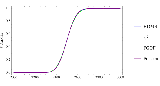
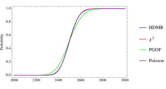
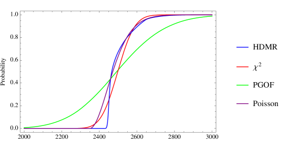
In Figure 1, we exhibit empirical distributions for PGOF, HDMR chi-square, and chi-square for kn=2500subscript𝑘𝑛2500k_{n}=2500 and n{50,500,5000}𝑛505005000n\in\{50,500,5000\}, having corresponding λ{1,10,100}𝜆110100\lambda\in\{1,10,100\}, for the power law distribution with α=1/2𝛼12\alpha=1/2. We show statistics for the estimators in Table 1. For λ=100𝜆100\lambda=100, Figure 1a shows both χn2superscriptsubscript𝜒𝑛2\chi_{n}^{2} and χnHDMR2superscriptsubscript𝜒𝑛HDMR2\chi_{n\text{HDMR}}^{2} are asymptotically χ2superscript𝜒2\chi^{2}. For λ=10𝜆10\lambda=10, Figure 1b shows that χn2superscriptsubscript𝜒𝑛2\chi_{n}^{2} is not asymptotically χ2superscript𝜒2\chi^{2} but χnHDMR2superscriptsubscript𝜒𝑛HDMR2\chi_{n\text{HDMR}}^{2} is. For λ=1𝜆1\lambda=1, Figure 1c shows that neither χn2superscriptsubscript𝜒𝑛2\chi_{n}^{2} nor χnHDMR2subscriptsuperscript𝜒2𝑛HDMR\chi^{2}_{n\text{HDMR}} is asymptotically χ2superscript𝜒2\chi^{2}. In particular, χnHDMR2subscriptsuperscript𝜒2𝑛HDMR\chi^{2}_{n\text{HDMR}} is expressed in terms of a Poisson law (see appendices for a precise characterization), although observe that the empirical distribution is truncated due to undersampling of the power law tails. The HDMR statistic χnHDMR2superscriptsubscript𝜒𝑛HDMR2\chi_{n\text{HDMR}}^{2} dominates the PGOF statistic χn2superscriptsubscript𝜒𝑛2\chi_{n}^{2}, i.e. PGOF experiences information leakage in comparison to the HDMR. For λ=1𝜆1\lambda=1 we observe PGOF to have a relative efficiency of 10%similar-toabsentpercent10\sim 10\% to that of HDMR.

Table 1: Estimator statistics from 5×1045superscript1045\times 10^{4} simulations for kn=2500subscript𝑘𝑛2500k_{n}=2500 and power law distribution with α=1/2𝛼12\alpha=1/2
𝔼𝔼\mathbb{E} 𝕍ar𝕍ar\mathbb{V}\text{ar}
n𝑛n knsubscript𝑘𝑛k_{n} λnkn𝜆𝑛subscript𝑘𝑛\lambda\equiv\frac{n}{\sqrt{k_{n}}} χn2superscriptsubscript𝜒𝑛2\chi_{n}^{2} χnHDMR2superscriptsubscript𝜒𝑛HDMR2\chi_{n\text{HDMR}}^{2} χn2superscriptsubscript𝜒𝑛2\chi_{n}^{2} χnHDMR2superscriptsubscript𝜒𝑛HDMR2\chi_{n\text{HDMR}}^{2}
5000 2 500 100 2499.20 2499.18 5464.45 5054.05
500 2 500 10 2498.84 2498.83 9023.85 5032.56
50 2 500 1 2499.30 2499.45 44188.40 5014.13
Refer to caption
(a) n=5000𝑛5000n=5000 (λ=100𝜆100\lambda=100)
Refer to caption
(b) n=500𝑛500n=500 (λ=10𝜆10\lambda=10)
Refer to caption
(c) n=50𝑛50n=50 (λ=1𝜆1\lambda=1)
Figure 1: Empirical distributions for kn=2500subscript𝑘𝑛2500k_{n}=2500 and power law distribution with α=1/2𝛼12\alpha=1/2

3.2 Reduced-order representation of high-dimensional behavior

Note that in this section we use ν𝜈\nu to indicate the measure on X𝑋X, and μ𝜇\mu and σ𝜎\sigma denote the mean and standard deviation common to the input variables.

In this application we compute HDMR for polynomial models, in particular the function i=1nxisuperscriptsubscriptproduct𝑖1𝑛subscript𝑥𝑖\prod_{i=1}^{n}x_{i} and a sum of elementary symmetric polynomials in n𝑛n variables. We show that the coefficient of variation ρ𝜌\rho of the input distribution ν𝜈\nu regulates the efficiency of low-dimensional HDMR approximations. We illustrate these properties for polynomial models.

Consider

f(x)=i=1nxi,iidx,ρσ/μ0formulae-sequence𝑓𝑥superscriptsubscriptproduct𝑖1𝑛subscript𝑥𝑖iid𝑥𝜌𝜎𝜇0f(x)=\prod_{i=1}^{n}x_{i},\;\;\;\text{iid}\,x,\;\;\;\rho\equiv\sigma/\mu\neq 0

with

𝕍arf=μ2n((1+ρ2)n1).𝕍ar𝑓superscript𝜇2𝑛superscript1superscript𝜌2𝑛1\mathbb{V}\text{ar}\,f=\mu^{2n}\left(\left(1+\rho^{2}\right)^{n}-1\right).

Per (3) the component functions of f(x)𝑓𝑥f(x) are

f0subscript𝑓0\displaystyle f_{0} =𝒫0f(x)=μnabsentsubscript𝒫0𝑓𝑥superscript𝜇𝑛\displaystyle=\mathscr{P}_{0}f(x)=\mu^{n}
fi(xi)subscript𝑓𝑖subscript𝑥𝑖\displaystyle f_{i}(x_{i}) =𝒫if(x)=μn1xif0absentsubscript𝒫𝑖𝑓𝑥superscript𝜇𝑛1subscript𝑥𝑖subscript𝑓0\displaystyle=\mathscr{P}_{i}f(x)=\mu^{n-1}x_{i}-f_{0}
fij(xi,xj)subscript𝑓𝑖𝑗subscript𝑥𝑖subscript𝑥𝑗\displaystyle f_{ij}(x_{i},x_{j}) =𝒫ijf(x)=μn2xixjfi(xi)fj(xj)f0absentsubscript𝒫𝑖𝑗𝑓𝑥superscript𝜇𝑛2subscript𝑥𝑖subscript𝑥𝑗subscript𝑓𝑖subscript𝑥𝑖subscript𝑓𝑗subscript𝑥𝑗subscript𝑓0\displaystyle=\mathscr{P}_{ij}f(x)=\mu^{n-2}x_{i}x_{j}-f_{i}(x_{i})-f_{j}(x_{j})-f_{0}
\displaystyle\vdots .

Employing the material in the appendices, the sensitivity indices satisfy

ki1<<ik𝕊i1ik=1subscript𝑘subscript𝑖1subscript𝑖𝑘subscript𝕊subscript𝑖1subscript𝑖𝑘1\sum_{\begin{subarray}{c}k\\ i_{1}<\dotsb<i_{k}\end{subarray}}\mathbb{S}_{i_{1}\dotsb i_{k}}=1

and at each order follow

p{k}i1<<ik𝕊i1ik𝑝𝑘subscriptsubscript𝑖1subscript𝑖𝑘subscript𝕊subscript𝑖1subscript𝑖𝑘\displaystyle p\{k\}\equiv\sum_{i_{1}<\dotsb<i_{k}}\mathbb{S}_{i_{1}\dotsb i_{k}} =(nk)ρ2k(ρ2+1)n1absentbinomial𝑛𝑘superscript𝜌2𝑘superscriptsuperscript𝜌21𝑛1\displaystyle=\frac{\binom{n}{k}\rho^{2k}}{\left(\rho^{2}+1\right)^{n}-1}

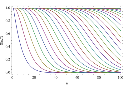
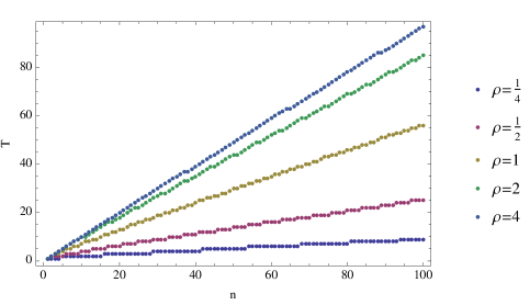
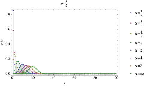
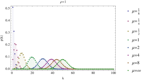
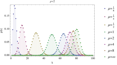
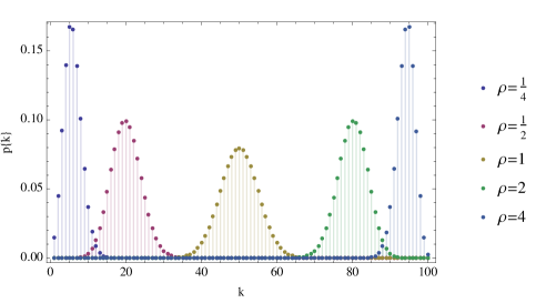
where kp{k}=1subscript𝑘𝑝𝑘1\sum_{k}p\{k\}=1. We have 𝔼p=nρ2(ρ2+1)n1(ρ2+1)n1𝔼𝑝𝑛superscript𝜌2superscriptsuperscript𝜌21𝑛1superscriptsuperscript𝜌21𝑛1\mathbb{E}\,p=\frac{n\rho^{2}\left(\rho^{2}+1\right)^{n-1}}{\left(\rho^{2}+1\right)^{n}-1} and 𝕍arp=nρ2(ρ2+1)n2((ρ2+1)nnρ21)((ρ2+1)n1)2𝕍ar𝑝𝑛superscript𝜌2superscriptsuperscript𝜌21𝑛2superscriptsuperscript𝜌21𝑛𝑛superscript𝜌21superscriptsuperscriptsuperscript𝜌21𝑛12\mathbb{V}\text{ar}\,p=\frac{n\rho^{2}\left(\rho^{2}+1\right)^{n-2}\left(\left(\rho^{2}+1\right)^{n}-n\rho^{2}-1\right)}{\left(\left(\rho^{2}+1\right)^{n}-1\right)^{2}}. Observe that when ρ<1𝜌1\rho<1 the explained variance of low dimensional approximations increases. For context, the uniform distribution on the unit interval (maximum entropy on [a,b]𝑎𝑏[a,b]) has ρ(Unif[0,1])=330.58𝜌Unif01330.58\rho(\text{Unif}[0,1])=\frac{\sqrt{3}}{3}\approx 0.58. In Figure 2, we plot the percent of explained variance by subspace order 𝒑(p{k}:kn)\bm{p}\equiv(p\{k\}:k\in\mathbb{N}_{n}) for n=100𝑛100n=100 and ρ{14,12,1,2,4}𝜌1412124\rho\in\{\frac{1}{4},\frac{1}{2},1,2,4\}. We observe that for ρ<1𝜌1\rho<1 the probability mass of the probability vector 𝒑𝒑\bm{p} is concentrated about small k𝑘k. Similar results are observed for sums of elementary symmetric polynomials in n𝑛n variables

En(x)=1+kni1<<ikxi1xik,subscript𝐸𝑛𝑥1subscript𝑘subscript𝑛subscript𝑖1subscript𝑖𝑘subscript𝑥subscript𝑖1subscript𝑥subscript𝑖𝑘E_{n}(x)=1+\sum_{\begin{subarray}{c}k\in\mathbb{N}_{n}\\ i_{1}<\dotsb<i_{k}\end{subarray}}x_{i_{1}}\dotsb\,x_{i_{k}},

where τσ1+μ𝜏𝜎1𝜇\tau\equiv\frac{\sigma}{1+\mu} regulates efficiency, and are contained in the appendices.
Refer to caption
Figure 2: p{k}=i1<<ik𝕊i1ik𝑝𝑘subscriptsubscript𝑖1subscript𝑖𝑘subscript𝕊subscript𝑖1subscript𝑖𝑘p\{k\}=\sum_{i_{1}<\dotsc<i_{k}}\mathbb{S}_{i_{1}\dotsc i_{k}}

We demonstrate this effect through Monte Carlo estimation of mean-squared-error test performance using the gradient boosting regressor (GBR) machine (Monte Carlo cross-validation), i.e. the generalization ability of the learning algorithm. We take n=10𝑛10n=10 and form D={(xi,f(xi))}i=1104Dsuperscriptsubscriptsubscript𝑥𝑖𝑓subscript𝑥𝑖𝑖1superscript104\textbf{D}=\{(x_{i},f(x_{i}))\}_{i=1}^{10^{4}} from iid random variables from a Beta(a,b)Beta𝑎𝑏\text{Beta}(a,b) distribution on X=[0,1]n𝑋superscript01𝑛X=[0,1]^{n}. For the beta distribution, we take ρ{14,12,1}𝜌14121\rho\in\{\frac{1}{4},\frac{1}{2},1\} using (a,b){(152,152),(32,32),(12,32)}𝑎𝑏15215232321232(a,b)\in\{(\frac{15}{2},\frac{15}{2}),(\frac{3}{2},\frac{3}{2}),(\frac{1}{2},\frac{3}{2})\}. We take a tree depth of six with 5×1035superscript1035\times 10^{3} trees. We split the data into training and test data. This is performed for 50 independent estimates, where (Di)subscriptD𝑖(\textbf{D}_{i}) are independently standardized using training data. Mean and standard deviation Monte Carlo estimates are shown below in Table 2 and density truth plots in Figure 3 (inverse-transformed): MSE markedly increases as ρ𝜌\rho increases.

Table 2: Monte Carlo MSE mean and standard deviation in p𝑝p
ρ𝜌\rho Mean Std
1/4 0.1207 0.0145
1/2 0.3866 0.1160
1 10.1248 45.55
Refer to caption
(a) ρ=14𝜌14\rho=\frac{1}{4}
Refer to caption
(b) ρ=12𝜌12\rho=\frac{1}{2}
Refer to caption
(c) ρ=1𝜌1\rho=1
Figure 3: Density truth plots for test data for ρ{14,12,1}𝜌14121\rho\in\{\frac{1}{4},\frac{1}{2},1\}

The total variable importance of xisubscript𝑥𝑖x_{i} to f𝑓f is computed as

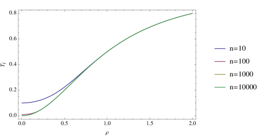
Ti=kρ2i(n1k1)(ρ2+1)n1=ρ2ρ2+1(ρ2+1)n(ρ2+1)n1ρ2ρ2+1.subscript𝑇𝑖subscript𝑘superscript𝜌2𝑖binomial𝑛1𝑘1superscriptsuperscript𝜌21𝑛1superscript𝜌2superscript𝜌21superscriptsuperscript𝜌21𝑛superscriptsuperscript𝜌21𝑛1superscript𝜌2superscript𝜌21T_{i}=\sum_{k}\frac{\rho^{2i}\binom{n-1}{k-1}}{\left(\rho^{2}+1\right)^{n}-1}=\frac{\rho^{2}}{\rho^{2}+1}\frac{\left(\rho^{2}+1\right)^{n}}{\left(\rho^{2}+1\right)^{n}-1}\approx\frac{\rho^{2}}{\rho^{2}+1}.

Observe that Tisubscript𝑇𝑖T_{i} is independent of the value of n𝑛n whenever n>k𝑛𝑘n>k for sufficiently large k𝑘k. This is depicted in Figure 4 and observed for k100similar-to𝑘100k\sim 100. Relative variable importance is trivially Ri=n1subscript𝑅𝑖superscript𝑛1R_{i}=n^{-1} and is independent of ρ𝜌\rho.

Refer to caption
Figure 4: Tisubscript𝑇𝑖T_{i} for (n,ρ){10,100,1000,10000}×[104,1]𝑛𝜌10100100010000superscript1041(n,\rho)\in\{10,100,1000,10000\}\times[10^{-4},1]

3.3 Analysis of variance for correlated input variables

Note that in this section and subsequent sections, we use μ𝜇\mu to indicate the probability measure on (X,𝒳)𝑋𝒳(X,\mathscr{X}).

In this application we show how variable importance I(f)I𝑓\text{I}(f) and variable dependence P(f)P𝑓\text{P}(f) by HDMR depend upon correlation ρ𝜌\rho in the input variables and this is necessary to preserve model variance. This provisions an analysis of variance that is consistent for correlated or degenerate input variables: total variance is preserved for all values of ρ𝜌\rho.

Let

F=L2(n,(n),μ)=ΠnSpan{xα:|α|n,α0n}𝐹superscript𝐿2superscript𝑛superscript𝑛𝜇superscriptΠ𝑛Spanconditional-setsuperscript𝑥𝛼formulae-sequence𝛼𝑛𝛼superscriptsubscript0𝑛F=L^{2}(\mathbb{R}^{n},\mathcal{B}(\mathbb{R}^{n}),\mu)=\Pi^{n}\equiv\text{Span}\{x^{\alpha}:|\alpha|\leq n,\,\alpha\in\mathbb{N}_{0}^{n}\}

where α=(α1,)𝛼subscript𝛼1\alpha=(\alpha_{1},\dotsc), |α|=iαi𝛼subscript𝑖subscript𝛼𝑖|\alpha|=\sum_{i}\alpha_{i}, and μ𝜇\mu is Gaussian. In particular, take n=2𝑛2n=2 and let

f(x)=β0+β1x1+β2x2+β12x1x2.𝑓𝑥subscript𝛽0subscript𝛽1subscript𝑥1subscript𝛽2subscript𝑥2subscript𝛽12subscript𝑥1subscript𝑥2f(x)=\beta_{0}+\beta_{1}x_{1}+\beta_{2}x_{2}+\beta_{12}x_{1}x_{2}. (2)

Its projections {fu𝒫uf}subscript𝑓𝑢subscript𝒫𝑢𝑓\{f_{u}\leftarrow\mathscr{P}_{u}f\} decompose f𝑓f,

f(x)=f0+f1(x1)+f2(x2)+f12(x1,x2),𝑓𝑥subscript𝑓0subscript𝑓1subscript𝑥1subscript𝑓2subscript𝑥2subscript𝑓12subscript𝑥1subscript𝑥2f(x)=f_{0}+f_{1}(x_{1})+f_{2}(x_{2})+f_{12}(x_{1},x_{2}),

where

f0subscript𝑓0\displaystyle f_{0} =β0+β1μ1+β2μ2+β12μ1μ2+β12ρσ1σ2absentsubscript𝛽0subscript𝛽1subscript𝜇1subscript𝛽2subscript𝜇2subscript𝛽12subscript𝜇1subscript𝜇2subscript𝛽12𝜌subscript𝜎1subscript𝜎2\displaystyle=\beta_{0}+\beta_{1}\mu_{1}+\beta_{2}\mu_{2}+\beta_{12}\mu_{1}\mu_{2}+\beta_{12}\rho\sigma_{1}\sigma_{2}
f1(x1)subscript𝑓1subscript𝑥1\displaystyle f_{1}(x_{1}) =(x1μ1)(β1+β12μ2)+(ρρ2+1)β12σ2σ1((x1μ1)2σ12)absentsubscript𝑥1subscript𝜇1subscript𝛽1subscript𝛽12subscript𝜇2𝜌superscript𝜌21subscript𝛽12subscript𝜎2subscript𝜎1superscriptsubscript𝑥1subscript𝜇12superscriptsubscript𝜎12\displaystyle=(x_{1}-\mu_{1})(\beta_{1}+\beta_{12}\mu_{2})+\left(\frac{\rho}{\rho^{2}+1}\right)\frac{\beta_{12}\sigma_{2}}{\sigma_{1}}\left((x_{1}-\mu_{1})^{2}-\sigma_{1}^{2}\right)
f2(x2)subscript𝑓2subscript𝑥2\displaystyle f_{2}(x_{2}) =(x2μ2)(β2+β12μ1)+(ρρ2+1)β12σ1σ2((x2μ2)2σ22)absentsubscript𝑥2subscript𝜇2subscript𝛽2subscript𝛽12subscript𝜇1𝜌superscript𝜌21subscript𝛽12subscript𝜎1subscript𝜎2superscriptsubscript𝑥2subscript𝜇22superscriptsubscript𝜎22\displaystyle=(x_{2}-\mu_{2})(\beta_{2}+\beta_{12}\mu_{1})+\left(\frac{\rho}{\rho^{2}+1}\right)\frac{\beta_{12}\sigma_{1}}{\sigma_{2}}\left((x_{2}-\mu_{2})^{2}-\sigma_{2}^{2}\right)
f12(x1,x2)subscript𝑓12subscript𝑥1subscript𝑥2\displaystyle f_{12}(x_{1},x_{2}) =β12(ρσ22((ρ21)σ12+(x1μ1)2)+(ρ2+1)σ1σ2(x1μ1)(x2μ2)+ρσ12((x2μ2)2))(ρ2+1)σ1σ2.absentsubscript𝛽12𝜌superscriptsubscript𝜎22superscript𝜌21superscriptsubscript𝜎12superscriptsubscript𝑥1subscript𝜇12superscript𝜌21subscript𝜎1subscript𝜎2subscript𝑥1subscript𝜇1subscript𝑥2subscript𝜇2𝜌superscriptsubscript𝜎12superscriptsubscript𝑥2subscript𝜇22superscript𝜌21subscript𝜎1subscript𝜎2\displaystyle=\frac{\beta_{12}\left(-\rho\sigma_{2}^{2}\left(\left(\rho^{2}-1\right)\sigma_{1}^{2}+(x_{1}-\mu_{1})^{2}\right)+\left(\rho^{2}+1\right)\sigma_{1}\sigma_{2}(x_{1}-\mu_{1})(x_{2}-\mu_{2})+\rho\sigma_{1}^{2}\left(-(x_{2}-\mu_{2})^{2}\right)\right)}{\left(\rho^{2}+1\right)\sigma_{1}\sigma_{2}}.

Computational details are contained in the appendices and these results are special cases of those in Li and Rabitz (2014). Observe that HDMR projections contain elements not observed in f𝑓f and that these additional elements are functions on X𝑋X that depend upon the parameters of μ𝜇\mu. For example, f1(x1)subscript𝑓1subscript𝑥1f_{1}(x_{1}) contains a quadratic term in x1subscript𝑥1x_{1}, whereas f(x)𝑓𝑥f(x) does not. The sensitivity indices of f𝑓f exhibit complex dependence on the model coefficients and distribution parameters,

𝕊1asubscriptsuperscript𝕊a1\displaystyle\mathbb{S}^{\text{a}}_{1} =σ12((β1+β12μ2)2+2β122ρ2σ22(ρ2+1)2)2ρσ1σ2(β1+β12μ2)(β2+β12μ1)+σ12(β1+β12μ2)2+σ22((β2+β12μ1)2+β122(ρ2+1)σ12)absentsuperscriptsubscript𝜎12superscriptsubscript𝛽1subscript𝛽12subscript𝜇222superscriptsubscript𝛽122superscript𝜌2superscriptsubscript𝜎22superscriptsuperscript𝜌2122𝜌subscript𝜎1subscript𝜎2subscript𝛽1subscript𝛽12subscript𝜇2subscript𝛽2subscript𝛽12subscript𝜇1superscriptsubscript𝜎12superscriptsubscript𝛽1subscript𝛽12subscript𝜇22superscriptsubscript𝜎22superscriptsubscript𝛽2subscript𝛽12subscript𝜇12superscriptsubscript𝛽122superscript𝜌21superscriptsubscript𝜎12\displaystyle=\frac{\sigma_{1}^{2}\left((\beta_{1}+\beta_{12}\mu_{2})^{2}+\frac{2\beta_{12}^{2}\rho^{2}\sigma_{2}^{2}}{\left(\rho^{2}+1\right)^{2}}\right)}{2\rho\sigma_{1}\sigma_{2}(\beta_{1}+\beta_{12}\mu_{2})(\beta_{2}+\beta_{12}\mu_{1})+\sigma_{1}^{2}(\beta_{1}+\beta_{12}\mu_{2})^{2}+\sigma_{2}^{2}\left((\beta_{2}+\beta_{12}\mu_{1})^{2}+\beta_{12}^{2}\left(\rho^{2}+1\right)\sigma_{1}^{2}\right)}
𝕊1bsubscriptsuperscript𝕊b1\displaystyle\mathbb{S}^{\text{b}}_{1} =ρσ1σ2((ρ2+1)2(β1+β12μ2)(β2+β12μ1)+2β122ρ3σ1σ2)(ρ2+1)2(2ρσ1σ2(β1+β12μ2)(β2+β12μ1)+σ12(β1+β12μ2)2+σ22((β2+β12μ1)2+β122(ρ2+1)σ12))absent𝜌subscript𝜎1subscript𝜎2superscriptsuperscript𝜌212subscript𝛽1subscript𝛽12subscript𝜇2subscript𝛽2subscript𝛽12subscript𝜇12superscriptsubscript𝛽122superscript𝜌3subscript𝜎1subscript𝜎2superscriptsuperscript𝜌2122𝜌subscript𝜎1subscript𝜎2subscript𝛽1subscript𝛽12subscript𝜇2subscript𝛽2subscript𝛽12subscript𝜇1superscriptsubscript𝜎12superscriptsubscript𝛽1subscript𝛽12subscript𝜇22superscriptsubscript𝜎22superscriptsubscript𝛽2subscript𝛽12subscript𝜇12superscriptsubscript𝛽122superscript𝜌21superscriptsubscript𝜎12\displaystyle=\frac{\rho\sigma_{1}\sigma_{2}\left(\left(\rho^{2}+1\right)^{2}(\beta_{1}+\beta_{12}\mu_{2})(\beta_{2}+\beta_{12}\mu_{1})+2\beta_{12}^{2}\rho^{3}\sigma_{1}\sigma_{2}\right)}{\left(\rho^{2}+1\right)^{2}\left(2\rho\sigma_{1}\sigma_{2}(\beta_{1}+\beta_{12}\mu_{2})(\beta_{2}+\beta_{12}\mu_{1})+\sigma_{1}^{2}(\beta_{1}+\beta_{12}\mu_{2})^{2}+\sigma_{2}^{2}\left((\beta_{2}+\beta_{12}\mu_{1})^{2}+\beta_{12}^{2}\left(\rho^{2}+1\right)\sigma_{1}^{2}\right)\right)}
𝕊12asubscriptsuperscript𝕊a12\displaystyle\mathbb{S}^{\text{a}}_{12} =β122(ρ21)2σ12σ22(ρ2+1)(2ρσ1σ2(β1+β12μ2)(β2+β12μ1)+σ12(β1+β12μ2)2+σ22((β2+β12μ1)2+β122(ρ2+1)σ12))absentsuperscriptsubscript𝛽122superscriptsuperscript𝜌212superscriptsubscript𝜎12superscriptsubscript𝜎22superscript𝜌212𝜌subscript𝜎1subscript𝜎2subscript𝛽1subscript𝛽12subscript𝜇2subscript𝛽2subscript𝛽12subscript𝜇1superscriptsubscript𝜎12superscriptsubscript𝛽1subscript𝛽12subscript𝜇22superscriptsubscript𝜎22superscriptsubscript𝛽2subscript𝛽12subscript𝜇12superscriptsubscript𝛽122superscript𝜌21superscriptsubscript𝜎12\displaystyle=\frac{\beta_{12}^{2}\left(\rho^{2}-1\right)^{2}\sigma_{1}^{2}\sigma_{2}^{2}}{\left(\rho^{2}+1\right)\left(2\rho\sigma_{1}\sigma_{2}(\beta_{1}+\beta_{12}\mu_{2})(\beta_{2}+\beta_{12}\mu_{1})+\sigma_{1}^{2}(\beta_{1}+\beta_{12}\mu_{2})^{2}+\sigma_{2}^{2}\left((\beta_{2}+\beta_{12}\mu_{1})^{2}+\beta_{12}^{2}\left(\rho^{2}+1\right)\sigma_{1}^{2}\right)\right)}
𝕊12bsubscriptsuperscript𝕊b12\displaystyle\mathbb{S}^{\text{b}}_{12} =0,absent0\displaystyle=0,

where

𝕊i=𝕊ia+𝕊ib,i{1,2,12}formulae-sequencesubscript𝕊𝑖subscriptsuperscript𝕊a𝑖subscriptsuperscript𝕊b𝑖𝑖1212\mathbb{S}_{i}=\mathbb{S}^{\text{a}}_{i}+\mathbb{S}^{\text{b}}_{i},\,\,\,i\in\{1,2,12\}

and satisfy for general parameters

𝕊1+𝕊2+𝕊12=1.subscript𝕊1subscript𝕊2subscript𝕊121\mathbb{S}_{1}+\mathbb{S}_{2}+\mathbb{S}_{12}=1.

Note that when ρ=0𝜌0\rho=0, then 𝕊1b=𝕊2b=𝕊12b=0subscriptsuperscript𝕊b1subscriptsuperscript𝕊b2subscriptsuperscript𝕊b120\mathbb{S}^{\text{b}}_{1}=\mathbb{S}^{\text{b}}_{2}=\mathbb{S}^{\text{b}}_{12}=0. All non-trivial projections depend upon ρ𝜌\rho and β𝛽\beta. In other words, the projections are functions of the measure μ𝜇\mu and of the model f𝑓f. Note that 𝕊12b=0subscriptsuperscript𝕊b120\mathbb{S}^{\text{b}}_{12}=0 for any ρ𝜌\rho due to the hierarchical-orthogonality of f12subscript𝑓12f_{12}, e.g., for every ρ𝜌\rho we have f12,f1=f12,f2=0subscript𝑓12subscript𝑓1subscript𝑓12subscript𝑓20\langle f_{12},f_{1}\rangle=\langle f_{12},f_{2}\rangle=0 but f1,f2=0subscript𝑓1subscript𝑓20\langle f_{1},f_{2}\rangle=0 only for ρ=0𝜌0\rho=0.

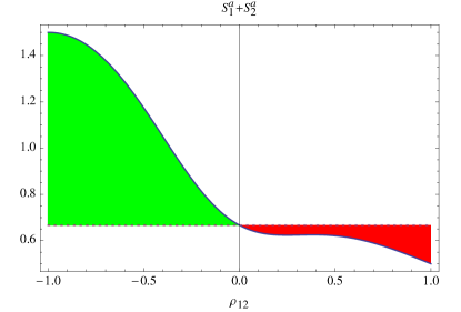
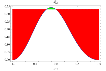
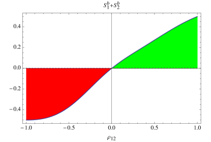
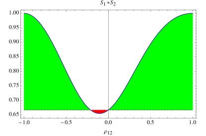
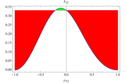
Consider ρ1𝜌1\rho\rightarrow 1. We know from the direct form of f(β,x)𝑓𝛽𝑥f(\beta,x) that in the limit we have x1=x2subscript𝑥1subscript𝑥2x_{1}=x_{2} and f(β,x)=β0+(β1+β2)x+β12x2𝑓𝛽𝑥subscript𝛽0subscript𝛽1subscript𝛽2𝑥subscript𝛽12superscript𝑥2f(\beta,x)=\beta_{0}+(\beta_{1}+\beta_{2})x+\beta_{12}x^{2}. That is, f𝑓f degenerates from a two-dimensional function into a one-dimensional function as the coherence indicated by ρ𝜌\rho achieves unity. HDMR uniquely captures this behavior in a variance-preserving manner for general distributions. We illustrate this property in Figure 5 with plots of the sensitivity indices as functions of ρ𝜌\rho for fixed μ𝜇\mu, σ𝜎\sigma and β𝛽\beta. Colored regions indicate increased variance (green) or reduced variance (red) relative to ρ=0𝜌0\rho=0. For example, Figure 5f illustrates that the HDMR component function subspace in X1×X2subscript𝑋1subscript𝑋2X_{1}\times X_{2} experiences annihilation for |ρ|1𝜌1|\rho|\rightarrow 1.

Refer to caption
(a) Structural, 𝕊1a+𝕊2asubscriptsuperscript𝕊a1subscriptsuperscript𝕊a2\mathbb{S}^{\text{a}}_{1}+\mathbb{S}^{\text{a}}_{2}
Refer to caption
(b) Structural, 𝕊12asubscriptsuperscript𝕊a12\mathbb{S}^{\text{a}}_{12}
Refer to caption
(c) Correlative, 𝕊1b+𝕊2bsubscriptsuperscript𝕊b1subscriptsuperscript𝕊b2\mathbb{S}^{\text{b}}_{1}+\mathbb{S}^{\text{b}}_{2}
Refer to caption
(d) Correlative, 𝕊12bsubscriptsuperscript𝕊b12\mathbb{S}^{\text{b}}_{12}
Refer to caption
(e) Overall, 𝕊1+𝕊2subscript𝕊1subscript𝕊2\mathbb{S}_{1}+\mathbb{S}_{2}
Refer to caption
(f) Overall, 𝕊12subscript𝕊12\mathbb{S}_{12}
Figure 5: sensitivity indices for β=𝟏𝛽1\beta=\bm{1}, μ=𝟎𝜇0\mu=\bm{0} and σ=𝟏𝜎1\sigma=\bm{1} as a function of ρ𝜌\rho, colored to reflect the correlative contributions (positive and negative)

In the next section we make a study of (2) using other interpretative diagnostics in machine learning and compare to the results of this section.

4 Interpretative diagnostics

Interpretative diagnostics provide explanation for prediction (Guyon and Elisseeff, 2003). Many common interpretative diagnostics are dependent upon the choice of F𝐹F and are said to be class-dependent. For example, variable depth in decision nodes of ensembles of decision trees and node weight pruning in neural networks are commonly employed for supervised machine learning settings to attain measures of variable importance. Other interpretative diagnostics are defined in terms of an objective function J𝐽J. For suitable J𝐽J finite differences or derivative-based sensitivity analysis are conducted to assess the importance of various subsets of variables. We use the risk function R𝑅R as the objective function J𝐽J. We compare variable importance and dependence measures using IusuperscriptI𝑢\textbf{I}^{u} and PusuperscriptP𝑢\textbf{P}^{u} defined by partial dependence (Friedman, 2001), derivative-based global sensitivity indices (Sobol’ and Kucherenko, 2009), and HDMR for the model (2). We illustrate that HDMR preserves explained variance independent of correlation in μ𝜇\mu, whereas partial dependence is valid for modest correlation (ρ<0.3𝜌0.3\rho<0.3).

4.1 Partial dependence

The partial dependence of f(x)𝑓𝑥f(x) on xusubscript𝑥𝑢x_{u} can be defined a couple ways (Friedman, 2001). One is given by

PPDuf(x)Muf(x)=Xuf(x)dμu(xu)=fuPD(xu),subscriptsuperscriptP𝑢PD𝑓𝑥superscriptM𝑢𝑓𝑥subscriptsubscript𝑋𝑢𝑓𝑥differential-dsubscript𝜇𝑢subscript𝑥𝑢subscriptsuperscript𝑓PD𝑢subscript𝑥𝑢{\color[rgb]{0,0,0}\textbf{P}^{u}_{\text{PD}}}f(x)\equiv\textbf{M}^{u}f(x)=\int_{X_{-u}}f(x)\mathrm{d}\mu_{-u}(x_{-u})={\color[rgb]{0,0,0}f^{\text{PD}}_{u}(x_{u})}, (3)

which is useful whenever the dependence between xusubscript𝑥𝑢x_{u} and xusubscript𝑥𝑢x_{-u} is not too strong. Another formulation of partial dependence is given by

PPDuf(x)Nuf(x)=Xuf(x)dμu|u(xu)=fuPD(xu),subscriptsuperscriptP𝑢PD𝑓𝑥superscriptN𝑢𝑓𝑥subscriptsubscript𝑋𝑢𝑓𝑥differential-dsubscript𝜇conditional𝑢𝑢subscript𝑥𝑢subscriptsuperscript𝑓PD𝑢subscript𝑥𝑢{\color[rgb]{0,0,0}\textbf{P}^{u}_{\text{PD}}}f(x)\equiv\textbf{N}^{u}f(x)=\int_{X_{-u}}f(x)\mathrm{d}\mu_{-u|u}(x_{-u})={\color[rgb]{0,0,0}f^{\text{PD}}_{u}(x_{u})}, (4)

which considers the effect of dependencies. Here, the function is averaged with respect to the conditional distribution. If f~(x)=f(x)f0~𝑓𝑥𝑓𝑥subscript𝑓0\tilde{f}(x)=f(x)-f_{0} and the inputs are independent, then partial dependence is related to HDMR, where PPDif~(x)=PHDMRif~(x)=f~iHDMR(xi)subscriptsuperscriptP𝑖PD~𝑓𝑥subscriptsuperscriptP𝑖HDMR~𝑓𝑥superscriptsubscript~𝑓𝑖HDMRsubscript𝑥𝑖\textbf{P}^{i}_{\text{PD}}\tilde{f}(x)=\textbf{P}^{i}_{\text{HDMR}}\tilde{f}(x)=\tilde{f}_{i}^{\text{HDMR}}(x_{i}) for in𝑖subscript𝑛i\in\mathbb{N}_{n}. Because of this relationship, we define the importance functional for partial dependence in a manner similar to HDMR,

IPDif(x)(SiaPD,SibPD,SiPD).subscriptsuperscriptI𝑖PD𝑓𝑥subscriptsuperscript𝑆𝑎PD𝑖subscriptsuperscript𝑆𝑏PD𝑖superscriptsubscript𝑆𝑖PD{\color[rgb]{0,0,0}\textbf{I}^{i}_{\text{PD}}}f(x)\equiv(S^{a\,\text{PD}}_{i},S^{b\,\text{PD}}_{i},S_{i}^{\text{PD}}).

4.2 Derivative-based global sensitivity measures

Sobol’ and Kucherenko (2009) introduced derivative-based global sensitivity measures. Weighted derivative-based global sensitivity measures (DGSM) are defined as

IDGSMuf(x)X(Dαuf(x))2wu(xu)dμ(x)=SuDGSM,subscriptsuperscriptI𝑢DGSM𝑓𝑥subscript𝑋superscriptsuperscript𝐷subscript𝛼𝑢𝑓𝑥2subscript𝑤𝑢subscript𝑥𝑢differential-d𝜇𝑥superscriptsubscript𝑆𝑢DGSM{\color[rgb]{0,0,0}\textbf{I}^{u}_{\text{DGSM}}}f(x)\equiv\int_{X}(D^{\alpha_{u}}f(x))^{2}w_{u}(x_{u})\mathrm{d}\mu(x)={\color[rgb]{0,0,0}S_{u}^{\text{DGSM}}},

where

Dαuf(x)=|α|f(x)x1αu1xnαunsuperscript𝐷subscript𝛼𝑢𝑓𝑥superscript𝛼𝑓𝑥superscriptsubscript𝑥1subscript𝛼𝑢1superscriptsubscript𝑥𝑛subscript𝛼𝑢𝑛D^{\alpha_{u}}f(x)=\frac{\partial^{|\alpha|}f(x)}{\partial x_{1}^{\alpha_{u1}}\dotsb\partial x_{n}^{\alpha_{un}}}

and wu(xu)subscript𝑤𝑢subscript𝑥𝑢w_{u}(x_{u}) is a weight function. Putting 𝑫𝜶𝒇=(Dαuf(x):u)\bm{D^{\alpha}f}=(D^{\alpha_{u}}f(x):u), a normalized DGSM is given as

IDGSMuf(x)X(Dαuf(x))2wu(xu)dμ(x)𝑫𝜶𝒇2;F2=SuDGSM,subscriptsuperscriptI𝑢DGSM𝑓𝑥subscript𝑋superscriptsuperscript𝐷subscript𝛼𝑢𝑓𝑥2subscript𝑤𝑢subscript𝑥𝑢differential-d𝜇𝑥superscriptsubscriptdelimited-∥∥superscript𝑫𝜶𝒇2𝐹2superscriptsubscript𝑆𝑢DGSM{\color[rgb]{0,0,0}\textbf{I}^{u}_{\text{DGSM}}}f(x)\equiv\frac{\int_{X}(D^{\alpha_{u}}f(x))^{2}w_{u}(x_{u})\mathrm{d}\mu(x)}{\lVert\bm{D^{\alpha}f}\rVert_{2;F}^{2}}={\color[rgb]{0,0,0}S_{u}^{\text{DGSM}}},

where

𝒇2;F=(f𝒇fL2(Ω,,μ)2)1/2.subscriptdelimited-∥∥𝒇2𝐹superscriptsubscript𝑓𝒇superscriptsubscriptdelimited-∥∥𝑓superscript𝐿2Ω𝜇212\lVert\bm{f}\rVert_{2;F}=\left(\sum_{f\in\bm{f}}\lVert f\rVert_{L^{2}(\Omega,\mathscr{F},\mu)}^{2}\right)^{1/2}.

We take wu(xu)=1subscript𝑤𝑢subscript𝑥𝑢1w_{u}(x_{u})=1.

4.3 Illustration

We illustrate these interpretative diagnostics for equation (2),

f(β,x)=β0+β1x1+β2x2+β12x1x2.𝑓𝛽𝑥subscript𝛽0subscript𝛽1subscript𝑥1subscript𝛽2subscript𝑥2subscript𝛽12subscript𝑥1subscript𝑥2f(\beta,x)=\beta_{0}+\beta_{1}x_{1}+\beta_{2}x_{2}+\beta_{12}x_{1}x_{2}.

We take β=𝟏𝛽1\beta=\bm{1}, μ=𝟏𝜇1\mu=\bm{1}, and σ=𝟏𝜎1\sigma=\bm{1}, and examine variable importance as a function of correlation, ρ𝜌\rho. For DGSM, we also consider σf2(β)=β22+2β2β3ρ+β32+β122(ρ2+1)superscriptsubscript𝜎𝑓2𝛽superscriptsubscript𝛽222subscript𝛽2subscript𝛽3𝜌superscriptsubscript𝛽32superscriptsubscript𝛽122superscript𝜌21\sigma_{f}^{2}(\beta)=\beta_{2}^{2}+2\beta_{2}\beta_{3}\rho+\beta_{3}^{2}+\beta_{12}^{2}\left(\rho^{2}+1\right). Whenever ρ{-1,1}𝜌-11\rho\in\{\text{-}1,1\} such that x1=x2subscript𝑥1subscript𝑥2x_{1}=x_{2} the function is one-dimensional and all variable importance resides in the univariate importance measures. The component functions are analytically given by

f~1HDMR(x1)superscriptsubscript~𝑓1HDMRsubscript𝑥1\displaystyle\tilde{f}_{1}^{\text{HDMR}}(x_{1}) =x1+ρρ2+1(x121)absentsubscript𝑥1𝜌superscript𝜌21superscriptsubscript𝑥121\displaystyle=x_{1}+\frac{\rho}{\rho^{2}+1}(x_{1}^{2}-1)
f~1PD (marg.)(x1)superscriptsubscript~𝑓1PD (marg.)subscript𝑥1\displaystyle\tilde{f}_{1}^{\text{PD (marg.)}}(x_{1}) =x1absentsubscript𝑥1\displaystyle=x_{1}
f~1PD (cond.)(x1)superscriptsubscript~𝑓1PD (cond.)subscript𝑥1\displaystyle\tilde{f}_{1}^{\text{PD (cond.)}}(x_{1}) =x1+ρ(x12+x11).absentsubscript𝑥1𝜌superscriptsubscript𝑥12subscript𝑥11\displaystyle=x_{1}+\rho(x_{1}^{2}+x_{1}-1).

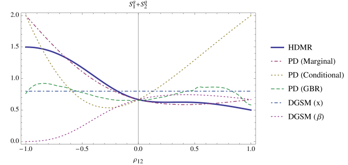
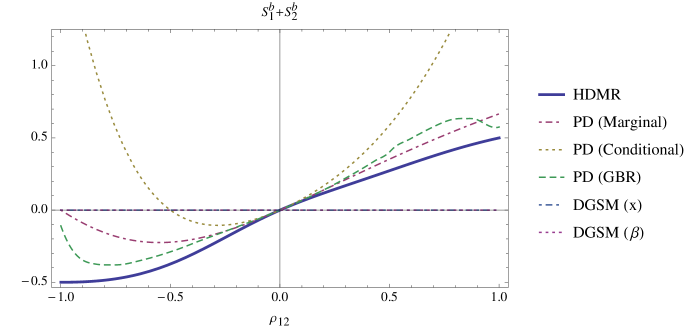
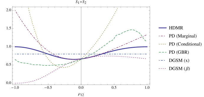
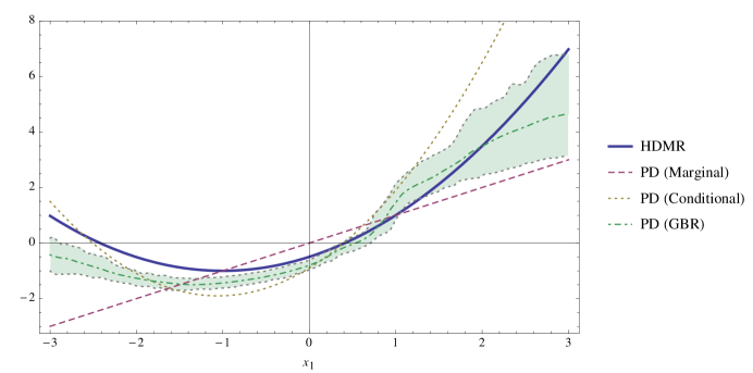
Notice that the HDMR component function has non-linear dependence on ρ𝜌\rho, whereas PD exhibits linear dependence. Variable importance results are exhibited in Table 3 and Figure 6 (note that the minimum and curvature for the ‘U’-shaped behavior changes in β𝛽\beta and for β=𝟏𝛽1\beta=\bm{1} in Figure 6c it is not symmetric), and variable dependence results are exhibited in Figure 7. For HDMR and partial dependence, we breakdown the importance measure into structural and correlative terms. We compute importance measures for ρ{-1,0,1}𝜌-101\rho\in\{\text{-}1,0,1\}. All importance measures, with the exception of IDGSMf(x)subscriptIDGSM𝑓𝑥\textbf{I}_{\text{DGSM}}f(x), depend upon ρ𝜌\rho. When ρ=0𝜌0\rho=0, all coincide except IDGSMf(x)subscriptIDGSM𝑓𝑥\textbf{I}_{\text{DGSM}}f(x). Only HDMR preserves variance, S(-1)=S(1)=1𝑆-1𝑆11S(\text{-}1)=S(1)=1.

The variance decomposition property of HDMR, i.e. S(-1)=S(1)=1𝑆-1𝑆11S(\text{-}1)=S(1)=1, means that the HDMR expansion correctly captures the contributions of subsets of variables to the variance in the output. Observe that partial dependence given by (3) is accurate when correlation is roughly less than 0.3. As the strength of dependence grows, the univariate partial dependency interpretative diagnostics of (3) become increasingly distorted. The diagnostic given by (4) exhibits far less variance stability in one-dimensional subspaces than that given by (3). PD is also estimated using a gradient boosting machine (PD (GBR), where GBR-estimated PD is estimated thirty times on a grid for ρ𝜌\rho, each GBR having 500 estimators of max depth of four and 103superscript10310^{3} independent random samples. PD (GBR) sensitivity indices are computed from the GBR-estimated PD’s using quadrature. GBR estimation of PD (3) is significantly biased as correlation increases. DGSM gives different importance of f(x)𝑓𝑥f(x) than HDMR and partial dependence, even for ρ=0𝜌0\rho=0, although it coincides for σf2(β)superscriptsubscript𝜎𝑓2𝛽\sigma_{f}^{2}(\beta).

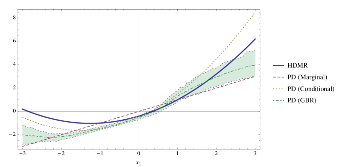
Figure 7 reveals the profile of f~1(x1)subscript~𝑓1subscript𝑥1\tilde{f}_{1}(x_{1}) in ρ𝜌\rho for HDMR and partial dependence (marginal, conditional, and GBR-estimated). PD (3) does not change in ρ𝜌\rho, whereas PD (4) does. PD (GBR) significantly deviates from both HDMR and PD (3). When ρ=0𝜌0\rho=0, the four coincide.

These results illustrate that PD-based interpretative diagnostics experience information leakage whenever ρ>0𝜌0\rho>0. In a similar manner, GBR-estimated PD exhibits information leakage. It is interesting that GBR-estimated PD diverges from both analytic PD-measures. This may be attributed to biases in the underlying algorthmic implementation, as tree-based ensemble methods such as random forest are known to exhibit biases in variable importance (Strobl et al., 2007).

Table 3: Variable importance measures in ρ𝜌\rho for β=𝟏𝛽1\beta=\bm{1}, μ=𝟏𝜇1\mu=\bm{1}, and σ=𝟏𝜎1\sigma=\bm{1}.
Variable Importance Sa(ρ)superscript𝑆a𝜌S^{\text{a}}(\rho) Sb(ρ)superscript𝑆b𝜌S^{\text{b}}(\rho) S(ρ)𝑆𝜌S(\rho) S(-1)𝑆-1S(\text{-}1) S(0)𝑆0S(0) S(1)𝑆1S(1)
IHDMR1subscriptsuperscriptI1HDMR\textbf{I}^{1}_{\text{HDMR}}+IHDMR2subscriptsuperscriptI2HDMR\textbf{I}^{2}_{\text{HDMR}} 2(ρ4+4ρ2+1)(ρ2+1)2(ρ(ρ+2)+3)2superscript𝜌44superscript𝜌21superscriptsuperscript𝜌212𝜌𝜌23\frac{2\left(\rho^{4}+4\rho^{2}+1\right)}{\left(\rho^{2}+1\right)^{2}(\rho(\rho+2)+3)} 2ρ(2ρ3+(ρ2+1)2)(ρ2+1)2(ρ(ρ+2)+3)2𝜌2superscript𝜌3superscriptsuperscript𝜌212superscriptsuperscript𝜌212𝜌𝜌23\frac{2\rho\left(2\rho^{3}+\left(\rho^{2}+1\right)^{2}\right)}{\left(\rho^{2}+1\right)^{2}(\rho(\rho+2)+3)} ρ1ρ2+1+ρ+5ρ(ρ+2)+3𝜌1superscript𝜌21𝜌5𝜌𝜌23\frac{\rho-1}{\rho^{2}+1}+\frac{\rho+5}{\rho(\rho+2)+3} 1 2/3 1
IPD1subscriptsuperscriptI1PD\textbf{I}^{1}_{\text{PD}}+IPD2subscriptsuperscriptI2PD\textbf{I}^{2}_{\text{PD}} (marg.) 2(ρ2+1)ρ(ρ+2)+32superscript𝜌21𝜌𝜌23\frac{2\left(\rho^{2}+1\right)}{\rho(\rho+2)+3} 2(ρ(ρ+1))ρ2+2ρ+32𝜌𝜌1superscript𝜌22𝜌3\frac{2(\rho(\rho+1))}{\rho^{2}+2\rho+3} 2(2ρ2+ρ+1)ρ(ρ+2)+322superscript𝜌2𝜌1𝜌𝜌23\frac{2\left(2\rho^{2}+\rho+1\right)}{\rho(\rho+2)+3} 2 2/3 4/3
IPD1subscriptsuperscriptI1PD\textbf{I}^{1}_{\text{PD}}+IPD2subscriptsuperscriptI2PD\textbf{I}^{2}_{\text{PD}} (cond.) 6ρ2+4ρ+2ρ2+2ρ+36superscript𝜌24𝜌2superscript𝜌22𝜌3\frac{6\rho^{2}+4\rho+2}{\rho^{2}+2\rho+3} 2(ρ(2ρ3+ρ2+2ρ+1))ρ2+2ρ+32𝜌2superscript𝜌3superscript𝜌22𝜌1superscript𝜌22𝜌3\frac{2\left(\rho\left(2\rho^{3}+\rho^{2}+2\rho+1\right)\right)}{\rho^{2}+2\rho+3} 2(ρ(ρ(2ρ2+ρ+5)+3)+1)ρ(ρ+2)+32𝜌𝜌2superscript𝜌2𝜌531𝜌𝜌23\frac{2\left(\rho\left(\rho\left(2\rho^{2}+\rho+5\right)+3\right)+1\right)}{\rho(\rho+2)+3} 4 2/3 4
IPD1subscriptsuperscriptI1PD\textbf{I}^{1}_{\text{PD}}+IPD2subscriptsuperscriptI2PD\textbf{I}^{2}_{\text{PD}} (GBR) - - - 0.65 0.65 1.14
IDGSM1subscriptsuperscriptI1DGSM\textbf{I}^{1}_{\text{DGSM}}+IDGSM2subscriptsuperscriptI2DGSM\textbf{I}^{2}_{\text{DGSM}} 4/5 0 4/5 4/5 4/5 4/5
IDGSM1subscriptsuperscriptI1DGSM\textbf{I}^{1}_{\text{DGSM}}+IDGSM2subscriptsuperscriptI2DGSM\textbf{I}^{2}_{\text{DGSM}} 2(ρ+1)2ρ(ρ3+4ρ+4)+32superscript𝜌12𝜌superscript𝜌34𝜌43\frac{2(\rho+1)^{2}}{\rho\left(\rho^{3}+4\rho+4\right)+3} 0 2(ρ+1)2ρ(ρ3+4ρ+4)+32superscript𝜌12𝜌superscript𝜌34𝜌43\frac{2(\rho+1)^{2}}{\rho\left(\rho^{3}+4\rho+4\right)+3} 0 2/3 2/3
Refer to caption
(a) Structural, S1a+S2asubscriptsuperscript𝑆a1subscriptsuperscript𝑆a2S^{\text{a}}_{1}+S^{\text{a}}_{2}
Refer to caption
(b) Correlative, S1b+S2bsubscriptsuperscript𝑆b1subscriptsuperscript𝑆b2S^{\text{b}}_{1}+S^{\text{b}}_{2}
Refer to caption
(c) Overall, S1+S2subscript𝑆1subscript𝑆2S_{1}+S_{2}
Figure 6: Univariate variable importance by HDMR, PD, and DGSM for β=𝟏𝛽1\beta=\bm{1}, μ=𝟎𝜇0\mu=\bm{0} and σ=𝟏𝜎1\sigma=\bm{1} as a function of ρ𝜌\rho.
Refer to caption
(a) ρ=0𝜌0\rho=0
Refer to caption
(b) ρ=12𝜌12\rho=\frac{1}{2}
Refer to caption
(c) ρ=910𝜌910\rho=\frac{9}{10}
Figure 7: Variable dependence f~1(x1)subscript~𝑓1subscript𝑥1\tilde{f}_{1}(x_{1}) for ρ{0,12,910}𝜌012910\rho\in\{0,\frac{1}{2},\frac{9}{10}\} for HDMR, PD (Marginal), PD (Conditional), and PD (GBR) ((α,1α)𝛼1𝛼(\alpha,1-\alpha) percentile, α=0.025𝛼0.025\alpha=0.025)

5 Glass boxes from black boxes

General-purpose black box learning algorithms in machine learning, such as kernel machines or decision tree models, exhibit favorable predictive performances and configuration or tuning costs. Suppose the availability of a black box representation fF𝑓𝐹f\in F. We demonstrate how HDMR assesses variable importance and dependence of kernel machines or ensembles of decision trees. In this manner, HDMR is said to be a wrapper method (Guyon and Elisseeff, 2003). We give HDMR constructions for kernel machines and ensembles of decision trees and provide illustrations for polynomial kernel machines and ensembles of gradient boosting machines.

5.1 Kernel machines

HDMR provide interpretative diagnostics for the output of a kernel machine through a decomposition of the inner product of its RKHS. This is similar to the approach used in smoothing spline ANOVA RKHS but such is based on orthogonal projections (Wahba, 1990; Wahba et al., 1995). We outline the approach below and discuss polynomial kernels.

Assume we have a kernel

K(x,x)=ϕ(x),ϕ(x)2,𝐾𝑥superscript𝑥subscriptbold-italic-ϕ𝑥bold-italic-ϕsuperscript𝑥superscript2K(x,x^{\prime})=\langle\bm{\phi}(x),\bm{\phi}(x^{\prime})\rangle_{\ell^{2}},

where ϕ:X2(𝜶):bold-italic-ϕmaps-to𝑋superscript2𝜶\bm{\phi}:X\mapsto\ell^{2}(\bm{\alpha}) is a feature map with index set 𝜶𝜶\bm{\alpha} of size b𝑏b\in\mathbb{N} and ϕ(x)=(ϕα(x):α𝜶)\bm{\phi}(x)=(\phi_{\alpha}(x):\alpha\in\bm{\alpha}) is a feature vector. We assume these feature vectors are represented by the Hadamard (entrywise) product of constants and basis elements, ϕ(x)=𝜷B(x)bold-italic-ϕ𝑥direct-product𝜷B𝑥\bm{\phi}(x)=\bm{\beta}\odot\textbf{B}(x), where B(x)=(Bα(x):α𝜶)\textbf{B}(x)=(\text{B}_{\alpha}(x):\alpha\in\bm{\alpha}) are bases and 𝜷b𝜷superscript𝑏\bm{\beta}\in\mathbb{R}^{b} are coefficients (note that B(x)B𝑥\textbf{B}(x) is known as a Mercer map). The HDMR of the kernel is attained by decomposing the feature vector as

ϕ(x)=α𝜶να𝝍α(x)=α𝜶να(𝜼αB(x)),bold-italic-ϕ𝑥subscript𝛼𝜶subscript𝜈𝛼subscript𝝍𝛼𝑥subscript𝛼𝜶subscript𝜈𝛼direct-productsubscript𝜼𝛼B𝑥\bm{\phi}(x)=\sum_{\alpha\in\bm{\alpha}}\nu_{\alpha}\bm{\psi}_{\alpha}(x)=\sum_{\alpha\in\bm{\alpha}}\nu_{\alpha}(\bm{\eta}_{\alpha}\odot\textbf{B}(x)), (5)

where {𝝍α(x)𝜼αB(x)}subscript𝝍𝛼𝑥direct-productsubscript𝜼𝛼B𝑥\{\bm{\psi}_{\alpha}(x)\equiv\bm{\eta}_{\alpha}\odot\textbf{B}(x)\} are component feature vectors and {𝜼α=(ηαα:α𝜶)}\{\bm{\eta}_{\alpha}=(\eta_{\alpha\alpha^{\prime}}:\alpha^{\prime}\in\bm{\alpha})\} are coefficient vectors attained from μ𝜇\mu. These coefficients reflect the hierarchical-orthogonality of the feature vectors and their generation is detailed in the appendices. Putting A(𝜼α)b×bAsubscript𝜼𝛼superscript𝑏𝑏\textbf{A}\equiv(\bm{\eta}_{\alpha})\in\mathbb{R}^{b\times b}, we have

𝜷=A𝝂𝜷A𝝂\bm{\beta}=\textbf{A}\,\bm{\nu} (6)

where 𝝂=(να:α𝜶)b\bm{\nu}=(\nu_{\alpha}:\alpha\in\bm{\alpha})\in\mathbb{R}^{b}. Given i) 𝜷𝜷\bm{\beta} from the kernel and ii) A from the measure μ𝜇\mu, this system is solved for 𝝂𝝂\bm{\nu},

𝝂=A1𝜷.𝝂superscriptA1𝜷\bm{\nu}=\textbf{A}^{-1}\bm{\beta}.

Using {να𝝍α(x)}subscript𝜈𝛼subscript𝝍𝛼𝑥\{\nu_{\alpha}\bm{\psi}_{\alpha}(x)\}, we form the HDMR of K𝐾\bm{K} by putting

ϕ(x)un𝚿u(x),italic-ϕ𝑥subscript𝑢subscript𝑛subscript𝚿𝑢𝑥\phi(x)\equiv\sum_{u\subseteq\mathbb{N}_{n}}\bm{\Psi}_{u}(x),

where the collection {𝚿u(x)}subscript𝚿𝑢𝑥\{\bm{\Psi}_{u}(x)\} is formed as

{𝚿u(x):un,𝜶u𝜶,𝚿u(x)α𝜶uνα𝝍α(x)}.conditional-setsubscript𝚿𝑢𝑥formulae-sequencefor-all𝑢subscript𝑛formulae-sequencesubscript𝜶𝑢𝜶subscript𝚿𝑢𝑥subscript𝛼subscript𝜶𝑢subscript𝜈𝛼subscript𝝍𝛼𝑥\left\{\bm{\Psi}_{u}(x):\forall u\subseteq\mathbb{N}_{n},\,\,\,\bm{\alpha}_{u}\subset\bm{\alpha},\,\,\,\bm{\Psi}_{u}(x)\equiv\sum_{\alpha\in\bm{\alpha}_{u}}\nu_{\alpha}\bm{\psi}_{\alpha}(x)\right\}. (7)

If a subset of component feature vectors is sought, {𝚿u(x):|u|T<d}conditional-setsubscript𝚿𝑢𝑥𝑢𝑇𝑑\{\bm{\Psi}_{u}(x):|u|\leq T<d\}, then we have Aa×bAsuperscript𝑎𝑏\textbf{A}\in\mathbb{R}^{a\times b}, an underdetermined system a<b𝑎𝑏a<b, and a least-norm solution can be efficiently attained using QR decomposition. Given a finite dataset D and a kernel K𝐾K, a kernel machine attains a set coefficients {ξx}subscript𝜉superscript𝑥\{\xi_{x^{\prime}}\} such that

f(x)𝑓𝑥\displaystyle f(x) =xDξxK(x,x)absentsubscriptsuperscript𝑥Dsubscript𝜉superscript𝑥𝐾𝑥superscript𝑥\displaystyle=\sum_{x^{\prime}\in\textbf{D}}\xi_{x^{\prime}}K(x,x^{\prime})
=xDξxϕ(x),ϕ(x)2absentsubscriptsuperscript𝑥Dsubscript𝜉superscript𝑥subscriptbold-italic-ϕ𝑥bold-italic-ϕsuperscript𝑥superscript2\displaystyle=\sum_{x^{\prime}\in\textbf{D}}\xi_{x^{\prime}}\langle\bm{\phi}(x),\bm{\phi}(x^{\prime})\rangle_{\ell^{2}}
=un𝚿u(x),xDξxϕ(x)2absentsubscriptsubscript𝑢subscript𝑛subscript𝚿𝑢𝑥subscriptsuperscript𝑥Dsubscript𝜉superscript𝑥bold-italic-ϕsuperscript𝑥superscript2\displaystyle=\left\langle\sum_{u\subseteq\mathbb{N}_{n}}\bm{\Psi}_{u}(x),\sum_{x^{\prime}\in\textbf{D}}\xi_{x^{\prime}}\bm{\phi}(x^{\prime})\right\rangle_{\ell^{2}}
=un𝚿u(x),f2absentsubscript𝑢subscript𝑛subscriptsubscript𝚿𝑢𝑥𝑓superscript2\displaystyle=\sum_{u\subseteq\mathbb{N}_{n}}\left\langle\bm{\Psi}_{u}(x),f\right\rangle_{\ell^{2}}
=unfuHDMR(xu).absentsubscript𝑢subscript𝑛subscriptsuperscript𝑓HDMR𝑢subscript𝑥𝑢\displaystyle=\sum_{u\subseteq\mathbb{N}_{n}}f^{\text{HDMR}}_{u}(x_{u}).

Polynomial kernels

The (real-valued) polynomial kernel is given by

Kpoly(x,x;c,d,γ)=(γxx+c)d,subscript𝐾poly𝑥superscript𝑥𝑐𝑑𝛾superscript𝛾𝑥superscript𝑥𝑐𝑑K_{\text{poly}}(x,x^{\prime};c,d,\gamma)=(\gamma x\cdot x^{\prime}+c)^{d}, (8)

where c,γ0𝑐𝛾0c,\gamma\geq 0, d𝑑d\in\mathbb{N}, and x,xn𝑥superscript𝑥superscript𝑛x,x^{\prime}\in\mathbb{R}^{n}. Defining 𝜶(n,d)={α0n+1,|α|=d}𝜶𝑛𝑑formulae-sequence𝛼superscriptsubscript0𝑛1𝛼𝑑\bm{\alpha}(n,d)=\{\alpha\in\mathbb{N}_{0}^{n+1},|\alpha|=d\},

B(x;n,d)=(xα1αn:α𝜶(n,d))\textbf{B}(x;n,d)=(x^{\alpha_{1}\dotsb\alpha_{n}}:\alpha\in\bm{\alpha}(n,d))

and

𝜷(n,d)=(βα:α𝜶(n,d)),\bm{\beta}(n,d)=(\beta_{\alpha}:\alpha\in\bm{\alpha}(n,d)),
βα=((dα)cα0γdα0)1/2,subscript𝛽𝛼superscriptbinomial𝑑𝛼superscript𝑐subscript𝛼0superscript𝛾𝑑subscript𝛼012\beta_{\alpha}=\left(\binom{d}{\alpha}c^{\alpha_{0}}\gamma^{d-\alpha_{0}}\right)^{1/2},

we have (suppressing notation in n𝑛n and d𝑑d)

ϕ(x)=𝜷B(x).bold-italic-ϕ𝑥direct-product𝜷B𝑥\bm{\phi}(x)=\bm{\beta}\odot\textbf{B}(x).

Together,

Kpoly(x,x;c,d,γ)subscript𝐾poly𝑥superscript𝑥𝑐𝑑𝛾\displaystyle K_{\text{poly}}(x,x^{\prime};c,d,\gamma) =ϕ(x),ϕ(x)2absentsubscriptbold-italic-ϕ𝑥bold-italic-ϕsuperscript𝑥superscript2\displaystyle=\langle\bm{\phi}(x),\bm{\phi}(x^{\prime})\rangle_{\ell^{2}}
=α𝜶βα2xα1αnxα1αn.absentsubscript𝛼𝜶superscriptsubscript𝛽𝛼2superscript𝑥subscript𝛼1subscript𝛼𝑛superscript𝑥subscript𝛼1subscript𝛼𝑛\displaystyle=\sum_{\alpha\in\bm{\alpha}}\beta_{\alpha}^{2}x^{\alpha_{1}\dotsb\alpha_{n}}x^{\prime\alpha_{1}\dotsb\alpha_{n}}.

Defining C(x;n,d)=(e2πiα1n,x:α𝜶(n,d))\textbf{C}(x;n,d)=(e^{2\pi i\langle\alpha_{1\dotsb n},x\rangle}:\alpha\in\bm{\alpha}(n,d)) and ϕ(x)=𝜷C(x)bold-italic-ϕ𝑥direct-product𝜷C𝑥\bm{\phi}(x)=\bm{\beta}\odot\textbf{C}(x), we write a complex-valued polynomial kernel,

Kpoly(x,x;c,d,γ)subscript𝐾poly𝑥superscript𝑥𝑐𝑑𝛾\displaystyle K_{\text{poly}}(x,x^{\prime};c,d,\gamma) =ϕ(x),ϕ(x)2absentsubscriptbold-italic-ϕ𝑥bold-italic-ϕsuperscript𝑥superscript2\displaystyle=\langle\bm{\phi}(x),\bm{\phi}(x^{\prime})\rangle_{\ell^{2}}
=(γe2πixe2πix+c)dabsentsuperscript𝛾superscript𝑒2𝜋𝑖𝑥superscript𝑒2𝜋𝑖superscript𝑥𝑐𝑑\displaystyle=(\gamma e^{2\pi ix}\cdot e^{2\pi ix^{\prime}}+c)^{d}
=α𝜶βα2e2πiα1n,xe2πiα1n,xabsentsubscript𝛼𝜶superscriptsubscript𝛽𝛼2superscript𝑒2𝜋𝑖subscript𝛼1𝑛𝑥superscript𝑒2𝜋𝑖subscript𝛼1𝑛superscript𝑥\displaystyle=\sum_{\alpha\in\bm{\alpha}}\beta_{\alpha}^{2}e^{2\pi i\langle\alpha_{1\dotsb n},x\rangle}e^{2\pi i\langle\alpha_{1\dotsb n},x^{\prime}\rangle}
=α𝜶βα2e2πiα1n,x+x.absentsubscript𝛼𝜶superscriptsubscript𝛽𝛼2superscript𝑒2𝜋𝑖subscript𝛼1𝑛𝑥superscript𝑥\displaystyle=\sum_{\alpha\in\bm{\alpha}}\beta_{\alpha}^{2}e^{2\pi i\langle\alpha_{1\dotsb n},x+x^{\prime}\rangle}.

Illustration: analytic function

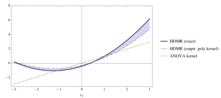
We consider the mathematical function (2). In Figure 8, we compare f1(x1)subscript𝑓1subscript𝑥1f_{1}(x_{1}) as computed by kernel machines—f1HDMR(x1)subscriptsuperscript𝑓HDMR1subscript𝑥1f^{\text{HDMR}}_{1}(x_{1}), attained from the empirical HDMR (16) (“empirical-polynomial HDMR”) and f1ANOVA(x1)subscriptsuperscript𝑓ANOVA1subscript𝑥1f^{\text{ANOVA}}_{1}(x_{1}), attained from the ANOVA representation of the polynomial kernel (8) (“ANOVA-polynomial kernel”). The ANOVA-kernel of the polynomial kernel is defined as KANOVA(x,x)=in(1+ki(xi,xi))subscript𝐾ANOVA𝑥superscript𝑥subscriptproduct𝑖subscript𝑛1subscript𝑘𝑖subscript𝑥𝑖superscriptsubscript𝑥𝑖K_{\text{ANOVA}}(x,x^{\prime})=\prod_{i\in\mathbb{N}_{n}}(1+k_{i}(x_{i},x_{i}^{\prime})) (Durrande et al., 2013), where {ki(xi,xi)}subscript𝑘𝑖subscript𝑥𝑖superscriptsubscript𝑥𝑖\{k_{i}(x_{i},x_{i}^{\prime})\} are univariate zero-mean polynomial kernels. Both kernel machines use the same empirical measure of 103superscript10310^{3} data elements with ρ=12𝜌12\rho=\frac{1}{2} and are compared to the exact HDMR. As seen in Figure 8, the ANOVA-polynomial kernel does not use the correlative information of the input data, whereas the empirical-polynomial HDMR better approximates the exact underlying HDMR.
Refer to caption
Figure 8: Plot of f1(x1)subscript𝑓1subscript𝑥1f_{1}(x_{1}) for ρ=12𝜌12\rho=\frac{1}{2}; HDMR (exact) compared to ANOVA-polynomial kernel and empirical-polynomial HDMR

5.2 Decision trees

A decision tree is a function that uses a partition of X=RiRRi𝑋subscriptsubscript𝑅𝑖𝑅subscript𝑅𝑖X=\cup_{R_{i}\in R}R_{i}, R={Ri}i𝑅subscriptsubscript𝑅𝑖𝑖R=\{R_{i}\}_{i}, such that

g(x)=RiRci1Ri(x).𝑔𝑥subscriptsubscript𝑅𝑖𝑅subscript𝑐𝑖subscript1subscript𝑅𝑖𝑥g(x)=\sum_{R_{i}\in R}c_{i}1_{R_{i}}(x).

The partition Rusubscript𝑅𝑢R_{u} is defined using a subset of variables xusubscript𝑥𝑢x_{u} such that a tree is written as

gu(xu)RiRuci1Ri(xu).subscript𝑔𝑢subscript𝑥𝑢subscriptsubscript𝑅𝑖subscript𝑅𝑢subscript𝑐𝑖subscript1subscript𝑅𝑖subscript𝑥𝑢g_{u}(x_{u})\equiv\sum_{R_{i}\in R_{u}}c_{i}1_{R_{i}}(x_{u}).

A collection of tree ensembles, indexed by \mathcal{I}, is denoted by

F{fi(x)}i,subscript𝐹subscriptsuperscript𝑓𝑖𝑥𝑖F_{\mathcal{I}}\equiv\{f^{i}(x)\}_{i\in\mathcal{I}}, (9)

where fi(x)superscript𝑓𝑖𝑥f^{i}(x) is a sum of trees across the subspaces 𝒫i(n)subscript𝒫𝑖Weierstrass-psubscript𝑛\mathcal{P}_{i}\subseteq\raisebox{1.79993pt}{\Large$\wp$}(\mathbb{N}_{n})

fi(x)u𝒫igui(xu)=u𝒫ijguji(xu)superscript𝑓𝑖𝑥subscript𝑢subscript𝒫𝑖subscriptsuperscript𝑔𝑖𝑢subscript𝑥𝑢subscript𝑢subscript𝒫𝑖subscript𝑗subscriptsuperscript𝑔𝑖𝑢𝑗subscript𝑥𝑢f^{i}(x)\equiv\sum_{u\in\mathcal{P}_{i}}g^{i}_{u}(x_{u})=\sum_{u\in\mathcal{P}_{i}}\sum_{j}g^{i}_{uj}(x_{u})

and has depth d𝑑d\in\mathbb{N} (Breiman, 2001). A key property of trained decision tree models is that tree subspaces are highly sparse, |𝒫i||(n)|much-less-thansubscript𝒫𝑖Weierstrass-psubscript𝑛|\mathcal{P}_{i}|\ll|\raisebox{1.79993pt}{\Large$\wp$}(\mathbb{N}_{n})| for in𝑖subscript𝑛i\in\mathbb{N}_{n}. A linear combination of tree ensembles is defined as

f(x)iβifi(x).𝑓𝑥subscript𝑖subscript𝛽𝑖superscript𝑓𝑖𝑥f(x)\equiv\sum_{i\in\mathcal{I}}\beta_{i}f^{i}(x). (10)

Forming 𝑭𝓘(fi:i)=(gui:i,u𝒫i)\bm{F_{\mathcal{I}}}\equiv(f^{i}:i\in\mathcal{I})=(g_{u}^{i}:i\in\mathcal{I},u\in\mathcal{P}_{i}) we take

𝜷(λ)(βui(λ):i,u𝒫i)=(𝑭𝓘𝑭𝓘+λI)1(𝑭𝓘f).\bm{\beta}(\lambda)\equiv(\beta_{ui}(\lambda):i\in\mathcal{I},u\in\mathcal{P}_{i})=(\bm{F_{\mathcal{I}}}\otimes\bm{F_{\mathcal{I}}}+\lambda I)^{-1}(\bm{F_{\mathcal{I}}}\otimes f).

We index the tree ensemble feature vectors on 𝜶𝜶\bm{\alpha} as

𝜶𝜶\displaystyle\bm{\alpha} (𝜶0)((i,u)×(n):i,u𝒫i)\displaystyle\equiv(\bm{\alpha}_{0})\parallel((i,u)\in\mathcal{I}\times\raisebox{1.79993pt}{\Large$\wp$}(\mathbb{N}_{n}):i\in\mathcal{I},\,\,\,u\in\mathcal{P}_{i})

where

𝜶0subscript𝜶0\displaystyle\bm{\alpha}_{0} =({},{})absent\displaystyle=(\{\},\{\})

and define

𝜶usubscript𝜶absent𝑢\displaystyle\bm{\alpha}_{\bullet u} {(i,w)𝜶:i,w=u}absentconditional-set𝑖𝑤𝜶formulae-sequence𝑖𝑤𝑢\displaystyle\equiv\{(i,w)\in\bm{\alpha}:i\in\mathcal{I},\,\,\,w=u\}
𝜶isubscript𝜶𝑖\displaystyle\bm{\alpha}_{i\bullet} {(j,u)𝜶:u𝒫j,j=i}.absentconditional-set𝑗𝑢𝜶formulae-sequence𝑢subscript𝒫𝑗𝑗𝑖\displaystyle\equiv\{(j,u)\in\bm{\alpha}:u\in\mathcal{P}_{j},\,\,\,j=i\}.

The tree ensemble feature vectors are given by

ϕi(x)superscriptbold-italic-ϕ𝑖𝑥\displaystyle\bm{\phi}^{i}(x) 𝜷i(λ)Bi(x)absentdirect-productsuperscript𝜷𝑖𝜆superscriptB𝑖𝑥\displaystyle\equiv\bm{\beta}^{i}(\lambda)\odot\textbf{B}^{i}(x)
Bi(x)superscriptB𝑖𝑥\displaystyle\textbf{B}^{i}(x) (gui(xu)1𝜶i(j,u):(j,u)𝜶)\displaystyle\equiv\left(g^{i}_{u}(x_{u})1_{\bm{\alpha}_{i\bullet}}(j,u):(j,u)\in\bm{\alpha}\right)
𝜷i(λ)superscript𝜷𝑖𝜆\displaystyle\bm{\beta}^{i}(\lambda) (βi(λ)1𝜶i(j,u):(j,u)𝜶).\displaystyle\equiv(\beta_{i}(\lambda)1_{\bm{\alpha}_{i\bullet}}(j,u):(j,u)\in\bm{\alpha}).

This is written as

ϕ(x)=i(𝜷i(λ)Bi(x))=𝜷(λ)B(x),bold-italic-ϕ𝑥subscript𝑖direct-productsuperscript𝜷𝑖𝜆superscriptB𝑖𝑥direct-product𝜷𝜆B𝑥\bm{\phi}(x)=\sum_{i\in\mathcal{I}}(\bm{\beta}^{i}(\lambda)\odot\textbf{B}^{i}(x))=\bm{\beta}(\lambda)\odot\textbf{B}(x),

where

B(x)=iBi(x)B𝑥subscript𝑖superscriptB𝑖𝑥\textbf{B}(x)=\sum_{i\in\mathcal{I}}\textbf{B}^{i}(x)

and

𝜷(λ)=i𝜷i(λ).𝜷𝜆subscript𝑖superscript𝜷𝑖𝜆\bm{\beta}(\lambda)=\sum_{i\in\mathcal{I}}\bm{\beta}^{i}(\lambda). (11)

Note that 𝜷0=0subscript𝜷00\bm{\beta}_{0}=0. As before, we have the coefficients attained from μ𝜇\mu as 𝜼αsubscript𝜼𝛼\bm{\eta}_{\alpha} and in organized form,

A(𝜼α).Asubscript𝜼𝛼\textbf{A}\equiv(\bm{\eta}_{\alpha}). (12)

Then, weights 𝝂=(να:α𝜶)\bm{\nu}=(\nu_{\alpha}:\alpha\in\bm{\alpha}) are attained that satisfy

𝜷(λ)=A𝝂𝜷𝜆A𝝂\bm{\beta}(\lambda)=\textbf{A}\,\bm{\nu} (13)

as

𝝂=A1𝜷(λ).𝝂superscriptA1𝜷𝜆\bm{\nu}=\textbf{A}^{-1}\bm{\beta}(\lambda). (14)

Noting

ϕ(x)=α𝜶να𝝍α(x)=α𝜶να(𝜼αB(x)),bold-italic-ϕ𝑥subscript𝛼𝜶subscript𝜈𝛼subscript𝝍𝛼𝑥subscript𝛼𝜶subscript𝜈𝛼direct-productsubscript𝜼𝛼B𝑥\bm{\phi}(x)=\sum_{\alpha\in\bm{\alpha}}\nu_{\alpha}\bm{\psi}_{\alpha}(x)=\sum_{\alpha\in\bm{\alpha}}\nu_{\alpha}(\bm{\eta}_{\alpha}\odot\textbf{B}(x)), (15)

we form the HDMR of Fsubscript𝐹\bm{F_{\mathcal{I}}} as

{𝚿u(x):un,𝜶u𝜶,𝚿u(x)α𝜶uνα𝝍α(x)}.conditional-setsubscript𝚿𝑢𝑥formulae-sequencefor-all𝑢subscript𝑛formulae-sequencesubscript𝜶𝑢𝜶subscript𝚿𝑢𝑥subscript𝛼subscript𝜶𝑢subscript𝜈𝛼subscript𝝍𝛼𝑥\left\{\bm{\Psi}_{u}(x):\forall u\subseteq\mathbb{N}_{n},\,\,\,\bm{\alpha}_{u}\subset\bm{\alpha},\,\,\,\bm{\Psi}_{u}(x)\equiv\sum_{\alpha\in\bm{\alpha}_{u}}\nu_{\alpha}\bm{\psi}_{\alpha}(x)\right\}. (16)

We summarize the computations:

  1. (i)

    Equation (9): forming Fsubscript𝐹F_{\mathcal{I}} from the collection of GBR models {fi(x)}isubscriptsuperscript𝑓𝑖𝑥𝑖\{f^{i}(x)\}_{i\in\mathcal{I}}, indexed on \mathcal{I}

  2. (ii)

    Equations (10) and (11): linearly combining the elements of Fsubscript𝐹F_{\mathcal{I}} as f(x)𝑓𝑥f(x) using the coefficients 𝜷(λ)(βui(λ):i,u𝒫i)b\bm{\beta}(\lambda)\equiv(\beta_{ui}(\lambda):i\in\mathcal{I},u\in\mathcal{P}_{i})\in\mathbb{R}^{\text{b}}, attained from regularized least-squares using with grid-searched λ𝜆\lambda estimated using K𝐾K-fold cross-validation

  3. (iii)

    Equation (12): attaining 𝜼αsubscript𝜼𝛼\bm{\eta}_{\alpha} from the measure μ𝜇\mu using a collection of QR-decompositions, each identified to a component function subspace and each QR decomposition having linear cost in the dataset size 𝒪(N)𝒪𝑁\mathcal{O}(N) and quadratic cost 𝒪(|𝒫(xu)𝒫i|2)𝒪superscript𝒫subscript𝑥𝑢subscript𝒫𝑖2\mathcal{O}(|\mathcal{P}(x_{u})\cap\mathcal{P}_{i}|^{2}) (typically small in most HDMR applications) and forming the square matrix Ab×bAsuperscript𝑏𝑏\textbf{A}\in\mathbb{R}^{b\times b}, where b𝑏b is total size of the corresponding inner product space |i𝒫i|subscript𝑖subscript𝒫𝑖|\cup_{i}\mathcal{P}_{i}|

  4. (iv)

    Equations (13) and (14): forming the system 𝜷=A𝝂𝜷A𝝂\bm{\beta}=\textbf{A}\cdot\bm{\nu}, computing the inverse of the square matrix A, such as through using Gaussian elimination, and putting 𝝂A1𝜷𝝂superscriptA1𝜷\bm{\nu}\equiv\textbf{A}^{-1}\bm{\beta}

  5. (v)

    Equations (15) and (16): forming the HDMR 𝑭𝓘subscript𝑭𝓘\bm{F_{\mathcal{I}}}.

Projections into the space of decision trees, which are systems of simple functions, produce noisy approximations to continuous functions. This can be addressed through spectral filtering of the component function subspaces, such as projection into smooth subspaces (Fourier). Another consideration is that if the GBR ensemble experience information leakage on the subspaces of F𝐹F the interpretative diagnostics will be biased (as illustrated in the previous section for non-trivial correlation). The variance-preserving property of HDMR, however, enables introspection of black box learning algorithms for independent and/or correlated variables, to the extent that the black box contains information on the projections of the system.

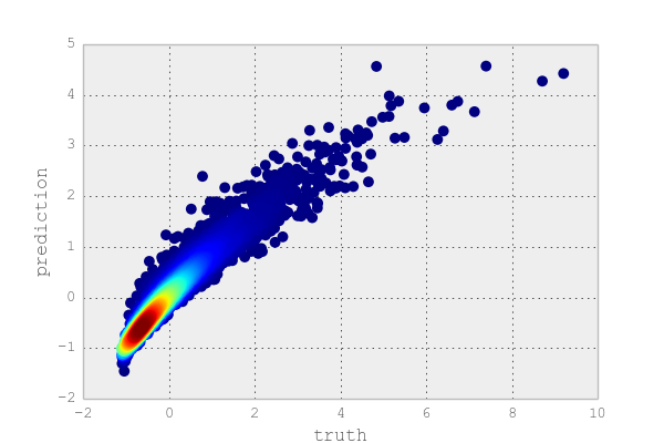
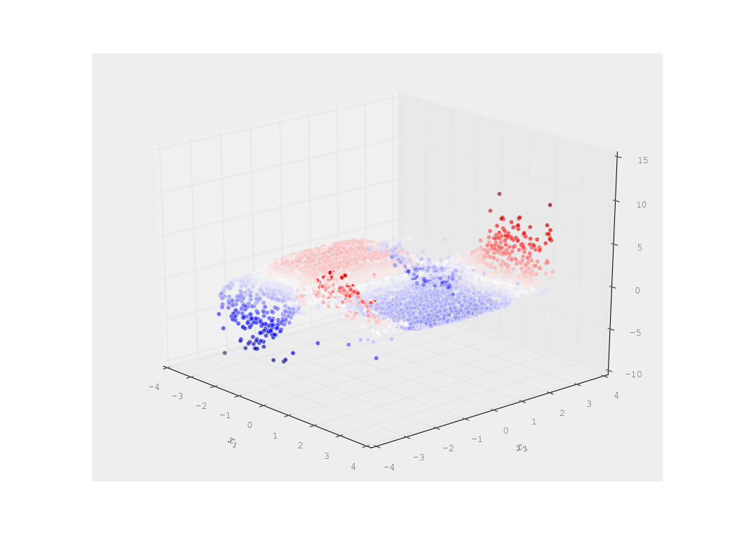
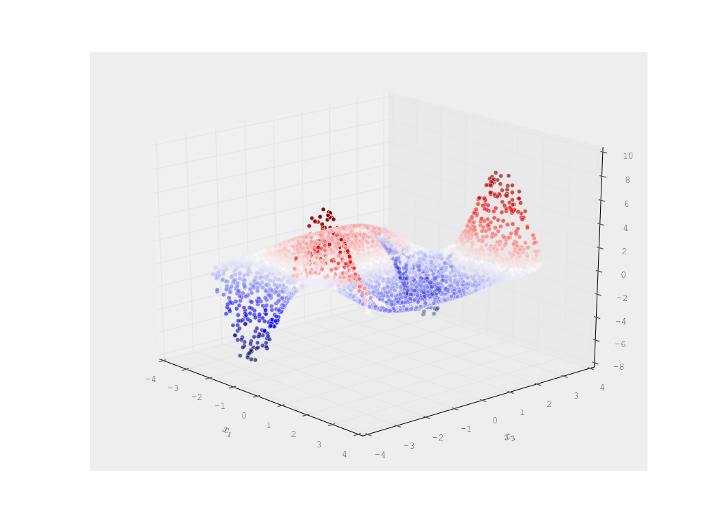
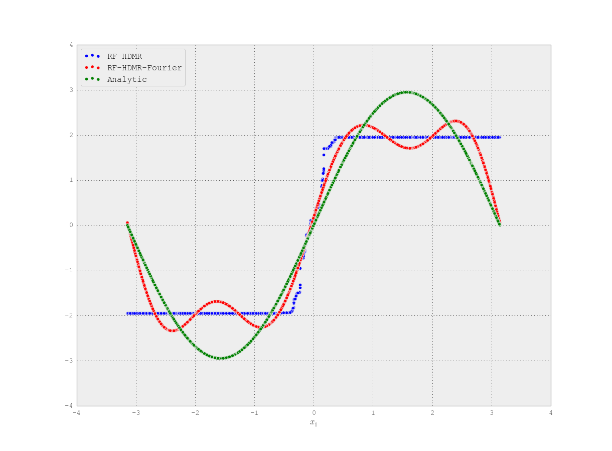
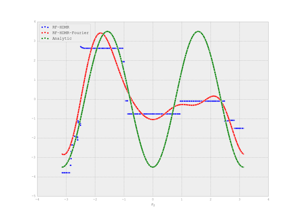
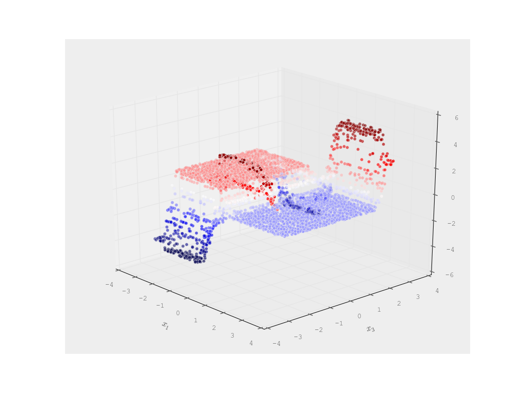
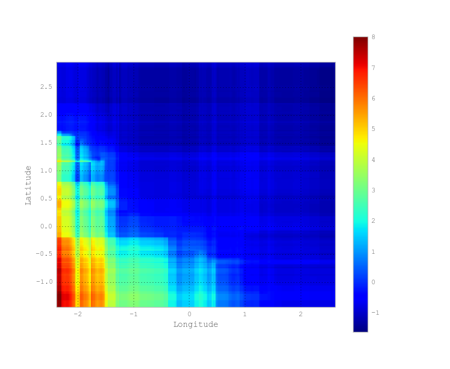
We compute the HDMR of two efficient general-purpose black-box supervised machine learning algorithms—the random forest (RF) and the gradient boosting regressor (GBR) machine—for a non-linear mathematical function (Ishigami) with analytic solution and a benchmark dataset (California housing). We demonstrate that RF experiences far more information leakage than GBR and that GBR well approximates HDMR.

Illustration 1: analytic test function

In this example we verify that the HDMR of Fsubscript𝐹F_{\mathcal{I}} given by (16) well approximates the true HDMR for a test function. We consider the Ishigami function, a non-linear continuous function, which exists in closed-form and is sparse. It is defined as

f(x)=sinx1+asin2x2+bx34sinx1𝑓𝑥subscript𝑥1𝑎superscript2subscript𝑥2𝑏superscriptsubscript𝑥34subscript𝑥1f(x)=\sin x_{1}+a\sin^{2}x_{2}+b\,x_{3}^{4}\sin x_{1}

with independent uniformly distributed x=(x1,x2,x3)[π,π]3𝑥subscript𝑥1subscript𝑥2subscript𝑥3superscript𝜋𝜋3x=(x_{1},x_{2},x_{3})\in[-\pi,\pi]^{3}. Its HDMR is analytic and shown below,

f0HDMRsubscriptsuperscript𝑓HDMR0\displaystyle f^{\text{HDMR}}_{0} =a2absent𝑎2\displaystyle=\frac{a}{2}
f1HDMR(x1)subscriptsuperscript𝑓HDMR1subscript𝑥1\displaystyle f^{\text{HDMR}}_{1}(x_{1}) =(1+bπ45)sinx1absent1𝑏superscript𝜋45𝑥1\displaystyle=(1+\frac{b\pi^{4}}{5})\sin x1
f2HDMR(x2)subscriptsuperscript𝑓HDMR2subscript𝑥2\displaystyle f^{\text{HDMR}}_{2}(x_{2}) =a2cos2x2absent𝑎22subscript𝑥2\displaystyle=-\frac{a}{2}\cos 2x_{2}
f3HDMR(x3)subscriptsuperscript𝑓HDMR3subscript𝑥3\displaystyle f^{\text{HDMR}}_{3}(x_{3}) =0absent0\displaystyle=0
f12HDMR(x1,x2)subscriptsuperscript𝑓HDMR12subscript𝑥1subscript𝑥2\displaystyle f^{\text{HDMR}}_{12}(x_{1},x_{2}) =0absent0\displaystyle=0
f13HDMR(x1,x3)subscriptsuperscript𝑓HDMR13subscript𝑥1subscript𝑥3\displaystyle f^{\text{HDMR}}_{13}(x_{1},x_{3}) =b(x34π45)sinx1absent𝑏superscriptsubscript𝑥34superscript𝜋45subscript𝑥1\displaystyle=b(x_{3}^{4}-\frac{\pi^{4}}{5})\sin x_{1}
f23HDMR(x2,x3)subscriptsuperscript𝑓HDMR23subscript𝑥2subscript𝑥3\displaystyle f^{\text{HDMR}}_{23}(x_{2},x_{3}) =0absent0\displaystyle=0
f123HDMR(x1,x2,x3)subscriptsuperscript𝑓HDMR123subscript𝑥1subscript𝑥2subscript𝑥3\displaystyle f^{\text{HDMR}}_{123}(x_{1},x_{2},x_{3}) =0.absent0\displaystyle=0.

Its non-trivial sensitivity indices are

𝕊1subscript𝕊1\displaystyle\mathbb{S}_{1} =36(π4b+5)25(45(a2+4)+20π8b2+72π4b)absent36superscriptsuperscript𝜋4𝑏52545superscript𝑎2420superscript𝜋8superscript𝑏272superscript𝜋4𝑏\displaystyle=\frac{36\left(\pi^{4}b+5\right)^{2}}{5\left(45\left(a^{2}+4\right)+20\pi^{8}b^{2}+72\pi^{4}b\right)}
𝕊2subscript𝕊2\displaystyle\mathbb{S}_{2} =45a245(a2+4)+20π8b2+72π4babsent45superscript𝑎245superscript𝑎2420superscript𝜋8superscript𝑏272superscript𝜋4𝑏\displaystyle=\frac{45a^{2}}{45\left(a^{2}+4\right)+20\pi^{8}b^{2}+72\pi^{4}b}
𝕊13subscript𝕊13\displaystyle\mathbb{S}_{13} =64π8b25(45(a2+4)+20π8b2+72π4b)absent64superscript𝜋8superscript𝑏2545superscript𝑎2420superscript𝜋8superscript𝑏272superscript𝜋4𝑏\displaystyle=\frac{64\pi^{8}b^{2}}{5\left(45\left(a^{2}+4\right)+20\pi^{8}b^{2}+72\pi^{4}b\right)}

We utilize an ensemble of GBR’s indexed on

isubscript𝑖\displaystyle\mathcal{I}_{i} ={(depthi,subspaces)}absentsubscriptdepth𝑖subspaces\displaystyle=\{(\text{depth}_{i},\text{subspaces})\}
={(k,(1,2,3)):k[i]}.absentconditional-set𝑘123𝑘delimited-[]𝑖\displaystyle=\{(k,(1,2,3)):k\in[i]\}.

These are linearly combined using regularized least-squares with grid-searched λ𝜆\lambda. J=103𝐽superscript103J=10^{3} trees are used in each ensemble and N=5×10³𝑁5superscript103N=5\times 10^{3} data points are sampled from Uniform[π,π]3Uniformsuperscript𝜋𝜋3\text{Uniform}[-\pi,\pi]^{3}.

In Figures 9 and 10 we estimate f1HDMR(x1)subscriptsuperscript𝑓HDMR1subscript𝑥1f^{\text{HDMR}}_{1}(x_{1}), f2HDMR(x2)subscriptsuperscript𝑓HDMR2subscript𝑥2f^{\text{HDMR}}_{2}(x_{2}), and f13HDMR(x1,x3)subscriptsuperscript𝑓HDMR13subscript𝑥1subscript𝑥3f^{\text{HDMR}}_{13}(x_{1},x_{3}) using GBR from F3subscript𝐹subscript3F_{\mathcal{I}_{3}}. We also estimate these using RF (located in the appendices; Figures 18, 19, and 20). We project the one-dimensional component functions into the space of zero-mean band-limited Fourier series (degree four) to attain smooth low-frequency approximations. Sensitivity indices are shown below in Table 4. The GBR-based decision tree approximations closely approximate the true HDMR component functions, whereas RF performs poorly, experiencing significant information leakage in comparison to GBR. GBR estimation of the two-dimensional component function f13HDMR(x1,x3)subscriptsuperscript𝑓HDMR13subscript𝑥1subscript𝑥3f^{\text{HDMR}}_{13}(x_{1},x_{3}) experiences some information leakage but its general qualitative behavior is satisfactorily reproduced as shown in Figure 10a. A tree-based measure of variable importance based on the fraction of samples variables contribute through trees is computed as ‘Tree’ and gives substantially different results than R𝑅R by HDMR: x3subscript𝑥3x_{3} is the most important variable by fraction of samples but the least important by HDMR. The defect in RF is appears to be insensitive to the number of trees, sample size, or tree depth.
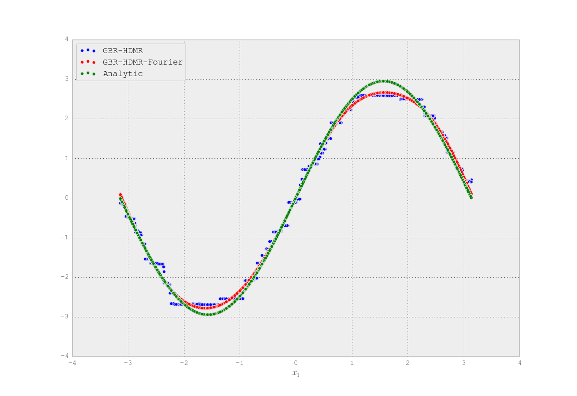
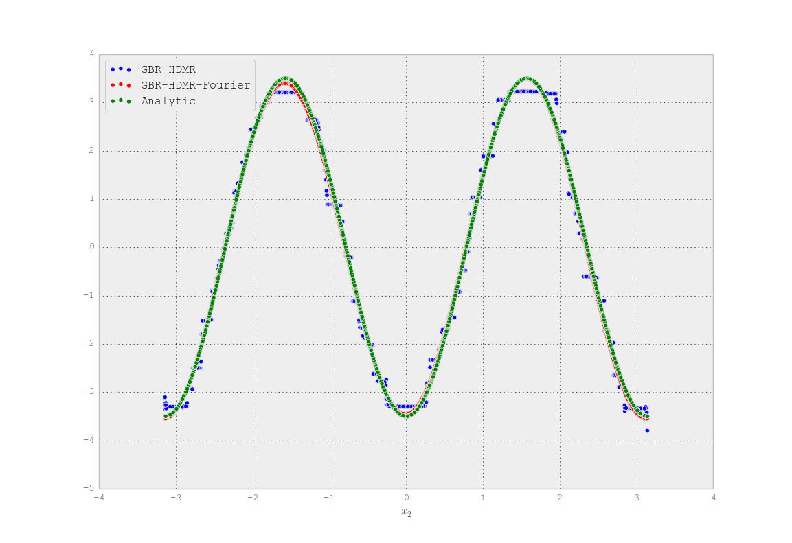
Figure 9: One-dimensional component functions: GBR approximation, smooth Fourier projection, and analytic
Refer to caption
(a) f1HDMR(x1)subscriptsuperscript𝑓HDMR1subscript𝑥1f^{\text{HDMR}}_{1}(x_{1})
Refer to caption
(b) f2HDMR(x2)subscriptsuperscript𝑓HDMR2subscript𝑥2f^{\text{HDMR}}_{2}(x_{2})
Figure 10: f13HDMR(x1,x3)subscriptsuperscript𝑓HDMR13subscript𝑥1subscript𝑥3f^{\text{HDMR}}_{13}(x_{1},x_{3}) by GBR approximation
Refer to caption
(a) Decision tree approximation
Refer to caption
(b) Analytic
Table 4: Structural and correlative sensitivity analysis PϵsubscriptPitalic-ϵ\text{P}_{\epsilon} for the Ishigami function (a=7𝑎7a=7, b=101𝑏superscript101b=10^{-1}) using gradient boosting regressor (GBR) machine and mean and standard deviation estimated from 50 random realizations for 1subscript1\mathcal{I}_{1}, 2subscript2\mathcal{I}_{2}, and 3subscript3\mathcal{I}_{3}
Subspace Index 𝕊asuperscript𝕊a\mathbb{S}^{\text{a}} 𝕊bsuperscript𝕊b\mathbb{S}^{\text{b}} 𝕊𝕊\mathbb{S} T R Tree
(1,) (Analytic) 0.31 0.00 0.31 0.56 0.45
1subscript1\mathcal{I}_{1} 0.31 ±plus-or-minus\pm 0.00 0.00 ±plus-or-minus\pm 0.00 0.31 ±plus-or-minus\pm 0.00 0.31 ±plus-or-minus\pm 0.00 0.40 ±plus-or-minus\pm 0.00 0.23 ±plus-or-minus\pm 0.00
2subscript2\mathcal{I}_{2} 0.29 ±plus-or-minus\pm 0.00 0.01 ±plus-or-minus\pm 0.00 0.30 ±plus-or-minus\pm 0.00 0.49 ±plus-or-minus\pm 0.01 0.42 ±plus-or-minus\pm 0.00 0.33 ±plus-or-minus\pm 0.01
3subscript3\mathcal{I}_{3} 0.29 ±plus-or-minus\pm 0.00 0.01 ±plus-or-minus\pm 0.00 0.30 ±plus-or-minus\pm 0.00 0.51 ±plus-or-minus\pm 0.01 0.42 ±plus-or-minus\pm 0.00 0.32 ±plus-or-minus\pm 0.01
(2,) (Analytic) 0.44 0.00 0.44 0.44 0.36
1subscript1\mathcal{I}_{1} 0.46 ±plus-or-minus\pm 0.00 -0.00 ±plus-or-minus\pm 0.00 0.45 ±plus-or-minus\pm 0.00 0.45 ±plus-or-minus\pm 0.00 0.58 ±plus-or-minus\pm 0.00 0.57 ±plus-or-minus\pm 0.00
2subscript2\mathcal{I}_{2} 0.44 ±plus-or-minus\pm 0.00 0.00 ±plus-or-minus\pm 0.00 0.45 ±plus-or-minus\pm 0.00 0.45 ±plus-or-minus\pm 0.00 0.38 ±plus-or-minus\pm 0.00 0.25 ±plus-or-minus\pm 0.01
3subscript3\mathcal{I}_{3} 0.44 ±plus-or-minus\pm 0.00 0.00 ±plus-or-minus\pm 0.00 0.45 ±plus-or-minus\pm 0.00 0.46 ±plus-or-minus\pm 0.00 0.38 ±plus-or-minus\pm 0.00 0.28 ±plus-or-minus\pm 0.01
(3,) (Analytic) 0.00 0.00 0.00 0.24 0.20
1subscript1\mathcal{I}_{1} 0.01 ±plus-or-minus\pm 0.00 0.00 ±plus-or-minus\pm 0.00 0.02 ±plus-or-minus\pm 0.00 0.02 ±plus-or-minus\pm 0.00 0.02 ±plus-or-minus\pm 0.00 0.21 ±plus-or-minus\pm 0.00
2subscript2\mathcal{I}_{2} 0.03 ±plus-or-minus\pm 0.00 0.01 ±plus-or-minus\pm 0.00 0.04 ±plus-or-minus\pm 0.01 0.23 ±plus-or-minus\pm 0.00 0.20 ±plus-or-minus\pm 0.00 0.42 ±plus-or-minus\pm 0.01
3subscript3\mathcal{I}_{3} 0.03 ±plus-or-minus\pm 0.00 0.01 ±plus-or-minus\pm 0.00 0.04 ±plus-or-minus\pm 0.01 0.25 ±plus-or-minus\pm 0.00 0.20 ±plus-or-minus\pm 0.00 0.40 ±plus-or-minus\pm 0.01
(1,2) (Analytic) 0.00 0.00 0.00
2subscript2\mathcal{I}_{2} 0.00 ±plus-or-minus\pm 0.00 -0.00 ±plus-or-minus\pm 0.00 0.00 ±plus-or-minus\pm 0.00
3subscript3\mathcal{I}_{3} 0.00 ±plus-or-minus\pm 0.00 -0.00 ±plus-or-minus\pm 0.00 0.00 ±plus-or-minus\pm 0.00
(1,3) (Analytic) 0.24 0.00 0.24
2subscript2\mathcal{I}_{2} 0.18 ±plus-or-minus\pm 0.00 0.01 ±plus-or-minus\pm 0.00 0.19 ±plus-or-minus\pm 0.00
3subscript3\mathcal{I}_{3} 0.19 ±plus-or-minus\pm 0.00 0.01 ±plus-or-minus\pm 0.00 0.20 ±plus-or-minus\pm 0.00
(2,3) (Analytic) 0.00 0.00 0.00
2subscript2\mathcal{I}_{2} 0.00 ±plus-or-minus\pm 0.00 0.00 ±plus-or-minus\pm 0.00 0.00 ±plus-or-minus\pm 0.00
3subscript3\mathcal{I}_{3} 0.00 ±plus-or-minus\pm 0.00 0.00 ±plus-or-minus\pm 0.00 0.00 ±plus-or-minus\pm 0.00
(1,2,3) (Analytic) 0.00 0.00 0.00
2subscript2\mathcal{I}_{2} 0.00 ±plus-or-minus\pm 0.00 -0.00 ±plus-or-minus\pm 0.00 0.00 ±plus-or-minus\pm 0.00
3subscript3\mathcal{I}_{3} 0.01 ±plus-or-minus\pm 0.00 0.00 ±plus-or-minus\pm 0.00 0.01 ±plus-or-minus\pm 0.00

Illustration 2: California housing dataset

We consider the California housing dataset. This dataset has nine variables, eight predictors and a single response variable ‘median house value.’ We standardize all variables to have zero mean and unit variance and utilize an ensemble of GBR’s indexed on

={(i,(1,,8)):i[3]},conditional-set𝑖18𝑖delimited-[]3\mathcal{I}=\{(i,(1,\dotsc,8)):i\in[3]\},

each having 5×1035superscript1035\times 10^{3} trees, to estimate the HDMR per (16).

Variable importance

We conduct a structural and correlative sensitivity analysis (SCSA) and show sensitivity indices with ϵ0.01italic-ϵ0.01\epsilon\geq 0.01 below in Table 5. Latitude and longitude each have strong negative correlative contributions to explained variance and participate in an modest-sized interaction. The relative sensitivity indices R (derived from the total T) are compared to the tree-based feature importance measure. HDMR places more emphasis on ‘MedInc’, ‘Latitude’, and ‘Longitude’ than the tree-based indices.

Table 5: Sensitivity analysis for the California housing dataset, PϵsubscriptPitalic-ϵ\text{P}_{\epsilon}, with ϵ=0.01italic-ϵ0.01\epsilon=0.01
Subspace Variables 𝕊asuperscript𝕊a\mathbb{S}^{\text{a}} 𝕊bsuperscript𝕊b\mathbb{S}^{\text{b}} 𝕊𝕊\mathbb{S} T R Tree
(1,) (’MedInc’,) 0.1346 0.1228 0.2574 0.3151 0.2637 0.1240
(2,) (’HouseAge’,) - - - 0.0377 0.0315 0.0612
(3,) (’AveRooms’,) 0.0305 0.0243 0.0548 0.0966 0.0808 0.1322
(4,) (’AveBedrms’,) - - - 0.0310 0.0259 0.0839
(5,) (’Population’,) - - - 0.0145 0.0121 0.0803
(6,) (’AveOccup’,) 0.0390 0.0168 0.0557 0.1310 0.1096 0.1475
(7,) (’Latitude’,) 0.7003 -0.5356 0.1646 0.2880 0.2411 0.1650
(8,) (’Longitude’,) 0.6585 -0.5218 0.1367 0.2810 0.2352 0.2058
(2, 6) (’HouseAge’, ’AveOccup’) 0.0069 0.0081 0.0150 - - -
(6, 8) (’AveOccup’, ’Longitude’) 0.0066 0.0046 0.0112 - - -
(7, 8) (’Latitude’, ’Longitude’) 0.0563 0.0168 0.0732 - - -
1.6374 -0.8562 0.7813 1.1948 1.00 1.00
One-dimensional variable dependence

Figures 11 and 22 show HDMR and partial dependence for ‘MedInc’, ‘Latitude’, and ’Longitude.’ HDMR and partial dependence are similar for ‘MedInc,’ although HDMR generally is smoother. For ’Latitude’ and ’Longitude’ they are somewhat different: HDMR profiles are generally vertically shifted to more negative values.
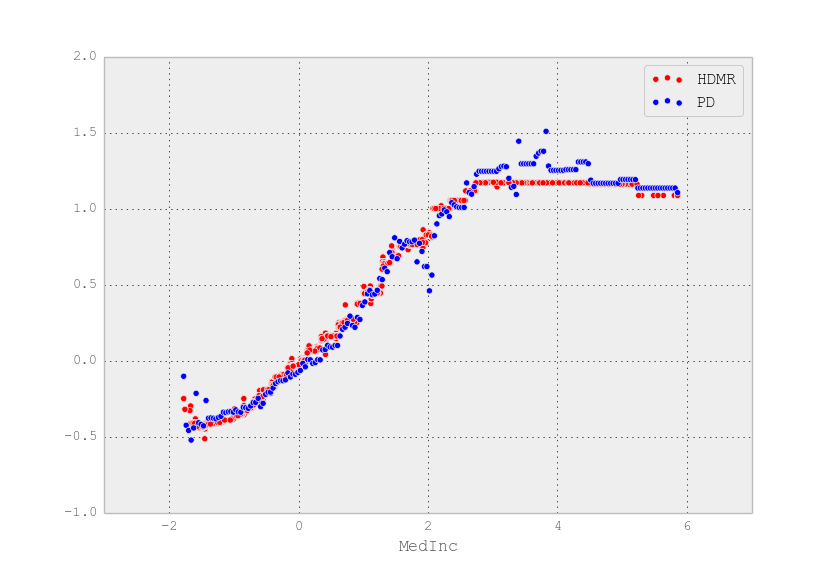
Refer to caption
Figure 11: HDMR and partial dependence for ‘MedInc’
Two-dimensional variable dependence

In Figure 12 we show the HDMR component function of latitude and longitude. In comparison to partial dependence (Figure 10.17 of Hastie et al. (2009)), HDMR reveals large positive values in scattered eastern localities and reveals positive contributions in northern-most and eastern-most locations.
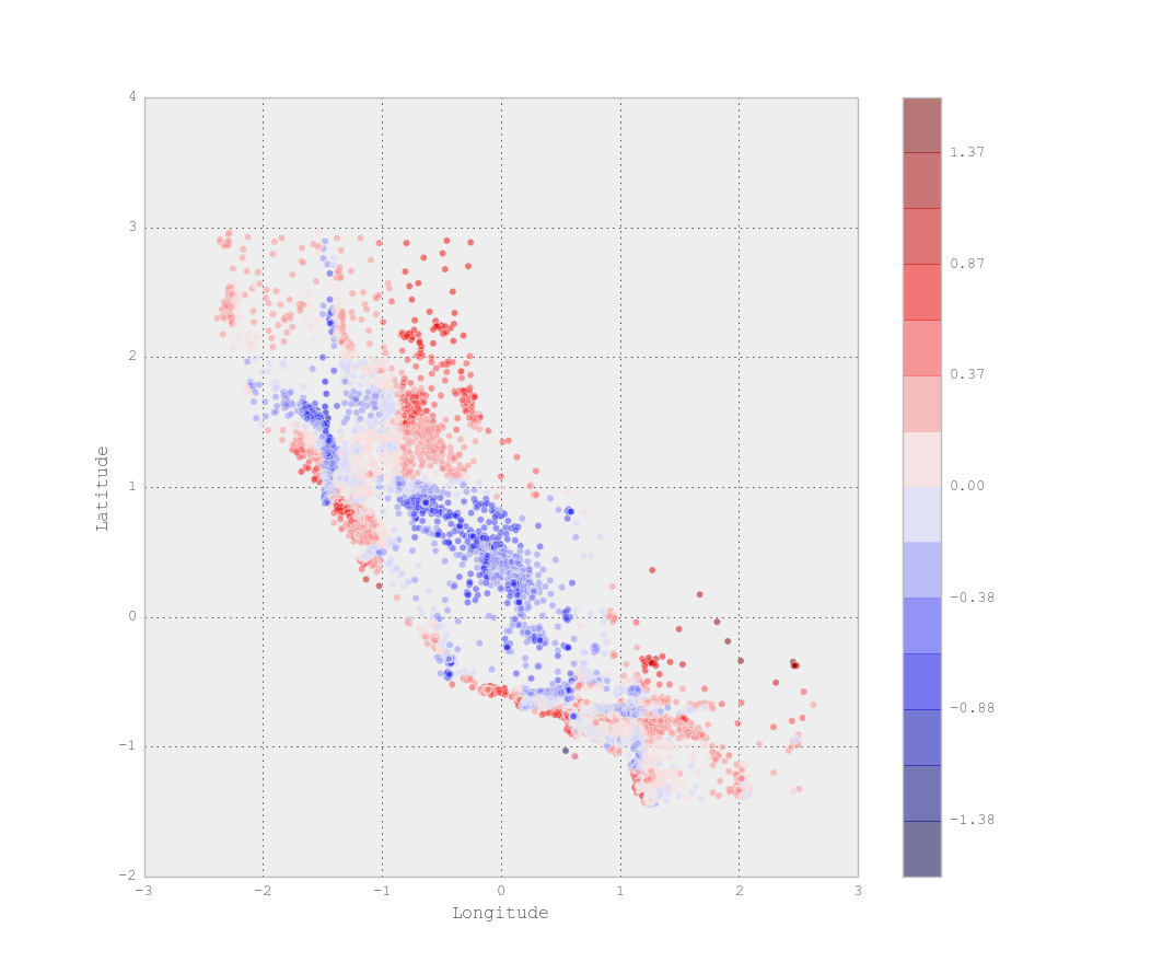
Refer to caption
Figure 12: HDMR component function in latitude and longitude

6 Concluding Remarks

HDMR provides structured information on the variable importance and dependence for square-integrable functions. As such, it provides information necessary and sufficient to interpret the model output in terms of the model input and constitutes a glass box representation. This research highlights key utilities of HDMR to supervised machine learning applications and introduces algorithmic constructions from black box models. One is that HDMR can identify sources of information leakage. This is demonstrated for goodness-of-fit settings for “big-data” and popular machine learning interpretative diagnostics and black boxes. Second, HDMR is a useful tool for managing the curse of dimensionality, as it often admits efficient reduced-order representations of dense high-dimensional systems. Third, whenever input variables are correlated, the HDMR component functions are functions of the input distribution parameters including those for correlation. Fourth, HDMR can be applied as a wrapper method for black boxes to provision glass boxes. Collectively, these results suggest HDMR to have broad utility within machine learning.

Acknowledgements

CB acknowledges support for this project from the National Institute of Dental and Craniofacial Research of the National Institutes of Health (NIH-NIDCR Grant No. K08-DE-021430). HR acknowledges support from the National Science Foundation. We thank Grzegorz A. Rempala for comments helpful to improving the article.

Computational implementations

PD (GBR) is computationally implemented using the scikit learn (version 0.18) classes GradientBoostingRegressor and partial-dependence.

Appendices

χn2superscriptsubscript𝜒𝑛2\chi_{n}^{2} decomposition

Recall the PGOF statistic

χn2=nk[kn](μ^n{k}μn{k})2μn{k}superscriptsubscript𝜒𝑛2𝑛subscript𝑘delimited-[]subscript𝑘𝑛superscriptsubscript^𝜇𝑛𝑘subscript𝜇𝑛𝑘2subscript𝜇𝑛𝑘\chi_{n}^{2}=n\sum_{k\in[k_{n}]}\frac{(\hat{\mu}_{n}\{k\}-\mu_{n}\{k\})^{2}}{\mu_{n}\{k\}}

with empirical probability μ^nsubscript^𝜇𝑛\hat{\mu}_{n} defined as

μ^n{k}=n1jnI(Xnj,k).subscript^𝜇𝑛𝑘superscript𝑛1subscript𝑗subscript𝑛𝐼subscript𝑋𝑛𝑗𝑘\hat{\mu}_{n}\{k\}=n^{-1}\sum_{j\in\mathbb{N}_{n}}I(X_{nj},k).

Put (x1,,xn)(Xn1,,Xnn)subscript𝑥1subscript𝑥𝑛subscript𝑋𝑛1subscript𝑋𝑛𝑛(x_{1},\dotsc,x_{n})\equiv(X_{n1},\dotsc,X_{nn}). Observe that the statistic χn2subscriptsuperscript𝜒2𝑛\chi^{2}_{n} is a function of the random observation vector (x1,,xn)subscript𝑥1subscript𝑥𝑛(x_{1},\dotsc,x_{n}). In Rempała and Wesołowski (2016) χn2superscriptsubscript𝜒𝑛2\chi_{n}^{2} is decomposed into two uncorrelated components,

χn2=n1(Sn+Un)n,superscriptsubscript𝜒𝑛2superscript𝑛1subscript𝑆𝑛subscript𝑈𝑛𝑛\chi_{n}^{2}=n^{-1}(S_{n}+U_{n})-n,

where

Sn=iμn1{xi}subscript𝑆𝑛subscript𝑖subscriptsuperscript𝜇1𝑛subscript𝑥𝑖S_{n}=\sum_{i}\mu^{-1}_{n}\{x_{i}\}

and

Un=i,jijμn1{xi}I(xi,xj)subscript𝑈𝑛subscript𝑖𝑗𝑖𝑗superscriptsubscript𝜇𝑛1subscript𝑥𝑖𝐼subscript𝑥𝑖subscript𝑥𝑗U_{n}=\sum_{\begin{subarray}{c}i,j\\ i\neq j\end{subarray}}\mu_{n}^{-1}\{x_{i}\}I(x_{i},x_{j})

with

𝔼Sn=nkn,𝔼Un=n(n1),𝔼χn2=kn1.formulae-sequence𝔼subscript𝑆𝑛𝑛subscript𝑘𝑛formulae-sequence𝔼subscript𝑈𝑛𝑛𝑛1𝔼superscriptsubscript𝜒𝑛2subscript𝑘𝑛1\mathbb{E}\,S_{n}=n\,k_{n},\,\,\,\,\,\mathbb{E}\,U_{n}=n(n-1),\,\,\,\,\,\mathbb{E}\,\chi_{n}^{2}=k_{n}-1.

This gives

𝕍arχn2=n1(𝕍arμn1{Xn}+2(n1)(kn1)).𝕍arsubscriptsuperscript𝜒2𝑛superscript𝑛1𝕍arsuperscriptsubscript𝜇𝑛1subscript𝑋𝑛2𝑛1subscript𝑘𝑛1\mathbb{V}\text{ar}\,\chi^{2}_{n}=n^{-1}\left(\mathbb{V}\text{ar}\,\mu_{n}^{-1}\{X_{n}\}+2(n-1)(k_{n}-1)\right).

This is a second-order HDMR,

χn2(x1,,xn)=f0+ifi(xi)+i<jfij(xi,xj),subscriptsuperscript𝜒2𝑛subscript𝑥1subscript𝑥𝑛subscript𝑓0subscript𝑖subscript𝑓𝑖subscript𝑥𝑖subscript𝑖𝑗subscript𝑓𝑖𝑗subscript𝑥𝑖subscript𝑥𝑗\chi^{2}_{n}(x_{1},\dotsc,x_{n})=f_{0}+\sum_{i}f_{i}(x_{i})+\sum_{i<j}f_{ij}(x_{i},x_{j}),

where

f0subscript𝑓0\displaystyle f_{0} =kn1absentsubscript𝑘𝑛1\displaystyle=k_{n}-1
fi(xi)subscript𝑓𝑖subscript𝑥𝑖\displaystyle f_{i}(x_{i}) =n1(μn1{xi}kn)absentsuperscript𝑛1superscriptsubscript𝜇𝑛1subscript𝑥𝑖subscript𝑘𝑛\displaystyle=n^{-1}\left(\mu_{n}^{-1}\{x_{i}\}-k_{n}\right)
fij(xi,xj)subscript𝑓𝑖𝑗subscript𝑥𝑖subscript𝑥𝑗\displaystyle f_{ij}(x_{i},x_{j}) =2n1(μn1{xi}I(xi,xj)1),absent2superscript𝑛1superscriptsubscript𝜇𝑛1subscript𝑥𝑖𝐼subscript𝑥𝑖subscript𝑥𝑗1\displaystyle=2\,n^{-1}\left(\mu_{n}^{-1}\{x_{i}\}\,I(x_{i},x_{j})-1\right),

with

𝕍arfi=n2𝕍arμn1{Xn}𝕍arsubscript𝑓𝑖superscript𝑛2𝕍arsuperscriptsubscript𝜇𝑛1subscript𝑋𝑛\mathbb{V}\text{ar}\,f_{i}=n^{-2}\,\mathbb{V}\text{ar}\,\mu_{n}^{-1}\{X_{n}\}

and

𝕍arfij=4n2(kn1).𝕍arsubscript𝑓𝑖𝑗4superscript𝑛2subscript𝑘𝑛1\mathbb{V}\text{ar}\,f_{ij}=4\,n^{-2}(k_{n}-1).

Note that if

(knn)1𝕍arμn1{Xn}n,kn0,𝑛subscript𝑘𝑛superscriptsubscript𝑘𝑛𝑛1𝕍arsuperscriptsubscript𝜇𝑛1subscript𝑋𝑛0(k_{n}n)^{-1}\mathbb{V}\text{ar}\,\mu_{\,n}^{-1}\{X_{n}\}\xrightarrow{n,k_{n}\rightarrow\infty}0,

then (2kn)1/2ifi(xi)0superscript2subscript𝑘𝑛12subscript𝑖subscript𝑓𝑖subscript𝑥𝑖0(2k_{n})^{-1/2}\sum_{i}f_{i}(x_{i})\rightarrow 0 in probability. This is satisfied for uniform and power law (α[0,1)𝛼01\alpha\in[0,1)) discrete random variables. Hence, for knsubscript𝑘𝑛k_{n}\rightarrow\infty as n𝑛n\rightarrow\infty, the first-order terms converge to constants and the asymptotic influence of the second-order terms dominates, i.e. the distributional limit of χn2superscriptsubscript𝜒𝑛2\chi_{n}^{2} is determined by the second-order component functions. This is equivalently stated using the sensitivity indices, i<j𝕊ijn,kn1𝑛subscript𝑘𝑛subscript𝑖𝑗subscript𝕊𝑖𝑗1\sum_{i<j}\mathbb{S}_{ij}\xrightarrow{n,k_{n}\rightarrow\infty}1. Putting n/knλ𝑛subscript𝑘𝑛𝜆n/\sqrt{k_{n}}\rightarrow\lambda, it turns out that χn2λ=Gaussian𝜆superscriptsubscript𝜒𝑛2Gaussian\chi_{n}^{2}\xrightarrow{\lambda=\infty}\text{Gaussian}, χn20<λ<Poisson0𝜆superscriptsubscript𝜒𝑛2Poisson\chi_{n}^{2}\xrightarrow{0<\lambda<\infty}\text{Poisson}, and χn2λ=0Degenerate𝜆0superscriptsubscript𝜒𝑛2Degenerate\chi_{n}^{2}\xrightarrow{\lambda=0}\text{Degenerate}. Hence, the distributional limit of χn2superscriptsubscript𝜒𝑛2\chi_{n}^{2} is standard Gaussian for (i) n,kn𝑛subscript𝑘𝑛n,k_{n}\rightarrow\inftywith λ=𝜆\lambda=\infty or for (ii) n𝑛n\rightarrow\inftyand kn=k<subscript𝑘𝑛𝑘k_{n}=k<\infty ; however, for n,kn𝑛subscript𝑘𝑛n,k_{n}\rightarrow\infty and λ<𝜆\lambda<\infty this is not true. Consequently, an improved statistic for χn2superscriptsubscript𝜒𝑛2\chi_{n}^{2} is defined using HDMR,

χnHDMR2(x1,,xn)superscriptsubscript𝜒𝑛HDMR2subscript𝑥1subscript𝑥𝑛\displaystyle\chi_{n\text{HDMR}}^{2}(x_{1},\dotsc,x_{n}) f0+i<jfij(xi,xj)absentsubscript𝑓0subscript𝑖𝑗subscript𝑓𝑖𝑗subscript𝑥𝑖subscript𝑥𝑗\displaystyle\equiv f_{0}+\sum_{i<j}f_{ij}(x_{i},x_{j})
χn2(x)ifi(xi).absentsuperscriptsubscript𝜒𝑛2𝑥subscript𝑖subscript𝑓𝑖subscript𝑥𝑖\displaystyle\equiv\chi_{n}^{2}(x)-\sum_{i}f_{i}(x_{i}).

A precise characterization of the asymptotic behavior of χn2superscriptsubscript𝜒𝑛2\chi_{n}^{2} is stated below. Note that this result also holds for power-law distributions.

Theorem 1 (Limit theorem for χn2superscriptsubscript𝜒𝑛2\chi_{n}^{2} for the uniform distribution).

Assume μn{x}=kn1subscript𝜇𝑛𝑥superscriptsubscript𝑘𝑛1\mu_{n}\{x\}=k_{n}^{-1} for xKn𝑥subscript𝐾𝑛x\in K_{n} and n=1,2,𝑛12n=1,2,\dotsc, as well as

n/knλ.𝑛subscript𝑘𝑛𝜆n/\sqrt{k_{n}}\rightarrow\lambda.

Then,

χn2kn2kn𝑑{0when λ=02λZλ2,ZPoisson(λ22)when λ(0,)NGaussian(0,1)when λ=.𝑑superscriptsubscript𝜒𝑛2subscript𝑘𝑛2subscript𝑘𝑛cases0when 𝜆0similar-to2𝜆𝑍𝜆2𝑍Poissonsuperscript𝜆22when 𝜆0similar-to𝑁Gaussian01when 𝜆\frac{\chi_{n}^{2}-k_{n}}{\sqrt{2k_{n}}}\xrightarrow{d}\begin{cases}0&\text{when }\lambda=0\\ \frac{\sqrt{2}}{\lambda}Z-\frac{\lambda}{\sqrt{2}},\,\,\,Z\sim\text{Poisson}\left(\frac{\lambda^{2}}{2}\right)&\text{when }\lambda\in(0,\infty)\\ N\sim\text{Gaussian}(0,1)&\text{when }\lambda=\infty.\end{cases}

Simple product function

For the function f(x)=i=1nxi𝑓𝑥superscriptsubscriptproduct𝑖1𝑛subscript𝑥𝑖f(x)=\prod_{i=1}^{n}x_{i}, the partition of variance is given by

𝕍ar(f)=σf2=iσi2+i<jσij2++σ1n2,𝕍ar𝑓superscriptsubscript𝜎𝑓2subscript𝑖superscriptsubscript𝜎𝑖2subscript𝑖𝑗superscriptsubscript𝜎𝑖𝑗2superscriptsubscript𝜎1𝑛2\color[rgb]{0,0,0}\mathbb{V}\text{ar}\,(f)=\sigma_{f}^{2}=\sum_{i}\sigma_{i}^{2}+\sum_{i<j}\sigma_{ij}^{2}+\dotsc+\sigma_{1\dotsc n}^{2},

where

σu2superscriptsubscript𝜎𝑢2\displaystyle\sigma_{u}^{2} =Xufu2(xu)dνu(xu)absentsubscriptsubscript𝑋𝑢subscriptsuperscript𝑓2𝑢subscript𝑥𝑢differential-dsubscript𝜈𝑢subscript𝑥𝑢\displaystyle=\int_{X_{u}}f^{2}_{u}(x_{u})\mathrm{d}\nu_{u}(x_{u})
νu(xu)subscript𝜈𝑢subscript𝑥𝑢\displaystyle\nu_{u}(x_{u}) =iuνi(xi)absentsubscriptproduct𝑖𝑢subscript𝜈𝑖subscript𝑥𝑖\displaystyle=\prod_{i\in u}\nu_{i}(x_{i})

and

σf2superscriptsubscript𝜎𝑓2\displaystyle{\color[rgb]{0,0,0}\sigma_{f}^{2}} =μ2n((1+ρ2)n1)absentsuperscript𝜇2𝑛superscript1superscript𝜌2𝑛1\displaystyle{\color[rgb]{0,0,0}\,\,=\mu^{2n}\left(\left(1+\rho^{2}\right)^{n}-1\right)}
σi2superscriptsubscript𝜎𝑖2\displaystyle\sigma_{i}^{2} =μ2nρ2absentsuperscript𝜇2𝑛superscript𝜌2\displaystyle=\mu^{2n}\rho^{2}
σij2superscriptsubscript𝜎𝑖𝑗2\displaystyle\sigma_{ij}^{2} =μ2nρ4absentsuperscript𝜇2𝑛superscript𝜌4\displaystyle=\mu^{2n}\rho^{4}
\displaystyle\vdots
σi1ik2superscriptsubscript𝜎subscript𝑖1subscript𝑖𝑘2\displaystyle{\color[rgb]{0,0,0}\sigma_{i_{1}\dotsb i_{k}}^{2}} =μ2nρ2k.absentsuperscript𝜇2𝑛superscript𝜌2𝑘\displaystyle{\color[rgb]{0,0,0}\,\,=\mu^{2n}\rho^{2k}}.

Figure 13 shows the percent of explained variance of fT(x1,,xn)superscript𝑓𝑇subscript𝑥1subscript𝑥𝑛f^{T}(x_{1},\dotsc,x_{n}) in (n,T)𝑛𝑇(n,T) for ρ=12𝜌12\rho=\frac{1}{2}. The curves correspond to different values of T𝑇T, where (1,,n)1𝑛(1,\dotsc,n) is left-to-right. As exhibited, increasing T𝑇T increases the explained variance.

Refer to caption
Figure 13: 𝕊(n,T)=k=1Tp{k}𝕊𝑛𝑇superscriptsubscript𝑘1𝑇𝑝𝑘\mathbb{S}(n,T)=\sum_{k=1}^{T}p\{k\} for (n,T){1,,100}2𝑛𝑇superscript11002(n,T)\in\{1,\dotsc,100\}^{2} and ρ=12𝜌12\rho=\frac{1}{2}

Figure 14 reveals that the necessary value of T𝑇T to attain a given percent of explained variance depends upon ρ𝜌\rho.

Refer to caption
Figure 14: minT𝑇\min T such that S(n,T)0.9𝑆𝑛𝑇0.9S(n,T)\geq 0.9 for (n,ρ){1,,100}×{14,12,1,2,4}𝑛𝜌11001412124(n,\rho)\in\{1,\dotsc,100\}\times\{\frac{1}{4},\frac{1}{2},1,2,4\}

Polynomials as linear combinations of monomials

Defining the monomial

xu=iuxisubscript𝑥𝑢subscriptproduct𝑖𝑢subscript𝑥𝑖x_{u}=\prod_{i\in u}x_{i}

with iid𝑖𝑖𝑑iid x𝑥x, having common μ𝜇\mu and σ2superscript𝜎2\sigma^{2}, we consider a linear combination of monomials,

eT(β,x)=u|u|Tβuxu.subscript𝑒𝑇𝛽𝑥subscript𝑢𝑢𝑇subscript𝛽𝑢subscript𝑥𝑢e_{T}(\beta,x)=\sum_{\begin{subarray}{c}u\\ |u|\leq T\end{subarray}}\beta_{u}x_{u}.

The variance of eTsubscript𝑒𝑇e_{T} is

𝕍ar(eT)=𝔼[(u|u|Tβu(xuμ|u|))2]=u|u|Tβu2𝕍ar(xu)+2u<v|u|,|v|Tβuβvov(xu,xv),𝕍arsubscript𝑒𝑇𝔼delimited-[]superscriptsubscript𝑢𝑢𝑇subscript𝛽𝑢subscript𝑥𝑢superscript𝜇𝑢2subscript𝑢𝑢𝑇superscriptsubscript𝛽𝑢2𝕍arsubscript𝑥𝑢2subscript𝑢𝑣𝑢𝑣𝑇subscript𝛽𝑢subscript𝛽𝑣ovsubscript𝑥𝑢subscript𝑥𝑣\mathbb{V}\text{ar}\,(e_{T})=\mathbb{E}[(\sum_{\begin{subarray}{c}u\\ |u|\leq T\end{subarray}}\beta_{u}(x_{u}-\mu^{|u|}))^{2}]=\sum_{\begin{subarray}{c}u\\ |u|\leq T\end{subarray}}\beta_{u}^{2}\mathbb{V}\text{ar}\,(x_{u})+2\sum_{\begin{subarray}{c}u<v\\ |u|,|v|\leq T\end{subarray}}\beta_{u}\beta_{v}\mathbb{C}\text{ov}(x_{u},x_{v}),

where, putting ρ=σ/μ𝜌𝜎𝜇\rho=\sigma/\mu,

𝕍ar(xu)=μ2|u|((1+ρ2)|u|1).𝕍arsubscript𝑥𝑢superscript𝜇2𝑢superscript1superscript𝜌2𝑢1\mathbb{V}\text{ar}\,(x_{u})=\mu^{2|u|}((1+\rho^{2})^{|u|}-1).
ov(xu,xv)=μ|u|+|v|((1+ρ2)|uv|1).ovsubscript𝑥𝑢subscript𝑥𝑣superscript𝜇𝑢𝑣superscript1superscript𝜌2𝑢𝑣1\mathbb{C}\text{ov}(x_{u},x_{v})=\mu^{|u|+|v|}((1+\rho^{2})^{|u\cap v|}-1).

eT(β,x)subscript𝑒𝑇𝛽𝑥e_{T}(\beta,x) is factorized as

eT(x)subscript𝑒𝑇𝑥\displaystyle e_{T}(x) =xi(u|u|T1|iu|=0βiuxu)+(u|u|T|iu|=0βuxu)absentsubscript𝑥𝑖subscript𝑢𝑢𝑇1𝑖𝑢0subscript𝛽𝑖𝑢subscript𝑥𝑢subscript𝑢𝑢𝑇𝑖𝑢0subscript𝛽𝑢subscript𝑥𝑢\displaystyle=x_{i}\left(\sum_{\begin{subarray}{c}u\\ |u|\leq T-1\\ |i\cap u|=0\end{subarray}}\beta_{iu}x_{u}\right)+\left(\sum_{\begin{subarray}{c}u\\ |u|\leq T\\ |i\cap u|=0\end{subarray}}\beta_{u}x_{u}\right)
=xij(u|u|T2|iju|=0βijuxu)+xi(u|u|T1|iju|=0βiuxu)+xj(u|u|T1|iju|=0βjuxu)+(u|u|T|iju|=0βuxu),absentsubscript𝑥𝑖𝑗subscript𝑢𝑢𝑇2𝑖𝑗𝑢0subscript𝛽𝑖𝑗𝑢subscript𝑥𝑢subscript𝑥𝑖subscript𝑢𝑢𝑇1𝑖𝑗𝑢0subscript𝛽𝑖𝑢subscript𝑥𝑢subscript𝑥𝑗subscript𝑢𝑢𝑇1𝑖𝑗𝑢0subscript𝛽𝑗𝑢subscript𝑥𝑢subscript𝑢𝑢𝑇𝑖𝑗𝑢0subscript𝛽𝑢subscript𝑥𝑢\displaystyle=x_{ij}\left(\sum_{\begin{subarray}{c}u\\ |u|\leq T-2\\ |ij\cap u|=0\end{subarray}}\beta_{iju}x_{u}\right)+x_{i}\left(\sum_{\begin{subarray}{c}u\\ |u|\leq T-1\\ |ij\cap u|=0\end{subarray}}\beta_{iu}x_{u}\right)+x_{j}\left(\sum_{\begin{subarray}{c}u\\ |u|\leq T-1\\ |ij\cap u|=0\end{subarray}}\beta_{ju}x_{u}\right)+\left(\sum_{\begin{subarray}{c}u\\ |u|\leq T\\ |ij\cap u|=0\end{subarray}}\beta_{u}x_{u}\right),

For β=𝟏𝛽1\beta=\bm{1}, we call eT(x)subscript𝑒𝑇𝑥e_{T}(x) an elementary symmetric polynomial and can compute its conditional expectations as

𝔼[eT]𝔼delimited-[]subscript𝑒𝑇\displaystyle\mathbb{E}[e_{T}] =a00absentsubscript𝑎00\displaystyle=a_{00}
𝔼[eT|i]𝔼delimited-[]conditionalsubscript𝑒𝑇subscript𝑖\displaystyle\mathbb{E}[e_{T}|\mathscr{F}_{i}] =a11xi+a10absentsubscript𝑎11subscript𝑥𝑖subscript𝑎10\displaystyle=a_{11}x_{i}+a_{10}
𝔼[eT|ij]𝔼delimited-[]conditionalsubscript𝑒𝑇subscript𝑖𝑗\displaystyle\mathbb{E}[e_{T}|\mathscr{F}_{ij}] =a22xij+a21(xi+xj)+a20.absentsubscript𝑎22subscript𝑥𝑖𝑗subscript𝑎21subscript𝑥𝑖subscript𝑥𝑗subscript𝑎20\displaystyle=a_{22}x_{ij}+a_{21}(x_{i}+x_{j})+a_{20}.
\displaystyle\vdots
𝔼[eT|u]𝔼delimited-[]conditionalsubscript𝑒𝑇subscript𝑢\displaystyle\mathbb{E}[e_{T}|\mathscr{F}_{u}] =wua|u||w|xw,absentsubscript𝑤𝑢subscript𝑎𝑢𝑤subscript𝑥𝑤\displaystyle=\sum_{w\subseteq u}a_{|u||w|}x_{w},

where

ars=u|u|Ts|ru|=0βruμ|u|=kTs(nrk)μk.subscript𝑎𝑟𝑠subscript𝑢𝑢𝑇𝑠𝑟𝑢0subscript𝛽𝑟𝑢superscript𝜇𝑢subscript𝑘𝑇𝑠binomial𝑛𝑟𝑘superscript𝜇𝑘a_{rs}=\sum_{\begin{subarray}{c}u\\ |u|\leq T-s\\ |r\cap u|=0\end{subarray}}\beta_{ru}\mu^{|u|}=\sum_{k\leq T-s}\binom{n-r}{k}\mu^{k}.

The component functions of eT(x)subscript𝑒𝑇𝑥e_{T}(x) are defined recursively,

f0subscript𝑓0\displaystyle f_{0} =𝔼[eT]absent𝔼delimited-[]subscript𝑒𝑇\displaystyle=\mathbb{E}[e_{T}]
fi(xi)subscript𝑓𝑖subscript𝑥𝑖\displaystyle f_{i}(x_{i}) =𝔼[eT|i]f0absent𝔼delimited-[]conditionalsubscript𝑒𝑇subscript𝑖subscript𝑓0\displaystyle=\mathbb{E}[e_{T}|\mathscr{F}_{i}]-f_{0}
fij(xi,xj)subscript𝑓𝑖𝑗subscript𝑥𝑖subscript𝑥𝑗\displaystyle f_{ij}(x_{i},x_{j}) =𝔼[eT|ij]fi(xi)fj(xj)f0absent𝔼delimited-[]conditionalsubscript𝑒𝑇subscript𝑖𝑗subscript𝑓𝑖subscript𝑥𝑖subscript𝑓𝑗subscript𝑥𝑗subscript𝑓0\displaystyle=\mathbb{E}[e_{T}|\mathscr{F}_{ij}]-f_{i}(x_{i})-f_{j}(x_{j})-f_{0}
\displaystyle\vdots
fu(xu)subscript𝑓𝑢subscript𝑥𝑢\displaystyle f_{u}(x_{u}) =𝔼[eT|u]wufw(xw).absent𝔼delimited-[]conditionalsubscript𝑒𝑇subscript𝑢subscript𝑤𝑢subscript𝑓𝑤subscript𝑥𝑤\displaystyle=\mathbb{E}[e_{T}|\mathscr{F}_{u}]-\sum_{w\subset u}f_{w}(x_{w}).

For T=n𝑇𝑛T=n, we have

σf2=(μ+1)2n((τ2+1)n1)superscriptsubscript𝜎𝑓2superscript𝜇12𝑛superscriptsuperscript𝜏21𝑛1\sigma_{f}^{2}=(\mu+1)^{2n}\left(\left(\tau^{2}+1\right)^{n}-1\right)
fu(xu)=(1+μ)n|u|iu(xiμ)subscript𝑓𝑢subscript𝑥𝑢superscript1𝜇𝑛𝑢subscriptproduct𝑖𝑢subscript𝑥𝑖𝜇f_{u}(x_{u})=(1+\mu)^{n-|u|}\prod_{i\in u}(x_{i}-\mu)
σu2=τ2|u|(μ+1)2nsubscriptsuperscript𝜎2𝑢superscript𝜏2𝑢superscript𝜇12𝑛\sigma^{2}_{u}=\tau^{2|u|}(\mu+1)^{2n}
q{k}=i1<<ik𝕊i1ik=(nk)τ2k(τ2+1)n1𝑞𝑘subscriptsubscript𝑖1subscript𝑖𝑘subscript𝕊subscript𝑖1subscript𝑖𝑘binomial𝑛𝑘superscript𝜏2𝑘superscriptsuperscript𝜏21𝑛1q\{k\}=\sum_{i_{1}<\dotsb<i_{k}}\mathbb{S}_{i_{1}\dotsc i_{k}}=\frac{\binom{n}{k}\tau^{2k}}{\left(\tau^{2}+1\right)^{n}-1}

where

τ=σμ+1=ρ1+1μ.𝜏𝜎𝜇1𝜌11𝜇\tau=\frac{\sigma}{\mu+1}=\frac{\rho}{1+\frac{1}{\mu}}.

When τ<1𝜏1\tau<1, q{k}>p{k}𝑞𝑘𝑝𝑘q\{k\}>p\{k\} for knmuch-less-than𝑘𝑛k\ll n. For the uniform distribution on the unit interval, we have τ=1330.19𝜏1330.19\tau=\frac{1}{3\sqrt{3}}\approx 0.19. Furthermore,

limμ,σσ/μ=ρτ=ρ.subscript𝜇𝜎𝜎𝜇𝜌𝜏𝜌\lim_{\begin{subarray}{c}\mu,\sigma\rightarrow\infty\\ \sigma/\mu=\rho\end{subarray}}\tau=\rho.
Refer to caption
Figure 15: q{k}=i1<<ik𝕊i1ik𝑞𝑘subscriptsubscript𝑖1subscript𝑖𝑘subscript𝕊subscript𝑖1subscript𝑖𝑘q\{k\}=\sum_{i_{1}<\dotsc<i_{k}}\mathbb{S}_{i_{1}\dotsc i_{k}} for ρ=12𝜌12\rho=\frac{1}{2}
Refer to caption
Figure 16: q{k}=i1<<ik𝕊i1ik𝑞𝑘subscriptsubscript𝑖1subscript𝑖𝑘subscript𝕊subscript𝑖1subscript𝑖𝑘q\{k\}=\sum_{i_{1}<\dotsc<i_{k}}\mathbb{S}_{i_{1}\dotsc i_{k}} for ρ=1𝜌1\rho=1
Refer to caption
Figure 17: q{k}=i1<<ik𝕊i1ik𝑞𝑘subscriptsubscript𝑖1subscript𝑖𝑘subscript𝕊subscript𝑖1subscript𝑖𝑘q\{k\}=\sum_{i_{1}<\dotsc<i_{k}}\mathbb{S}_{i_{1}\dotsc i_{k}} for ρ=2𝜌2\rho=2

Feature vector construction for hierarchically-orthogonal subspaces

Suppose for the measure space (Xu,𝒳u,μu)subscript𝑋𝑢subscript𝒳𝑢subscript𝜇𝑢(X_{u},\mathscr{X}_{u},\mu_{u}) of subspace u{1,,n}𝑢1𝑛u\subseteq\{1,\dotsc,n\}, where μu(xu)=Xuμ(xu,dxu)subscript𝜇𝑢subscript𝑥𝑢subscriptsuperscript𝑋𝑢𝜇subscript𝑥𝑢dsubscript𝑥𝑢\mu_{u}(x_{u})=\int_{X^{-u}}\mu(x_{u},\mathrm{d}x_{-u}), we have a collection of basis vectors indexed on (u)Weierstrass-p𝑢\raisebox{1.79993pt}{\Large$\wp$}(u) and having dimensions b=(bv:v(u))b=(b_{v}\in\mathbb{N}:v\in\raisebox{1.79993pt}{\Large$\wp$}(u)). This is denoted by

B{Bv(Bv1,,Bvbv):v(u)}.Bconditional-setsubscriptB𝑣subscriptB𝑣1subscriptB𝑣subscript𝑏𝑣𝑣Weierstrass-p𝑢\textbf{B}\equiv\{\text{B}_{v}\equiv(\text{B}_{v1},\dotsc,\text{B}_{vb_{v}}):v\in\raisebox{1.79993pt}{\Large$\wp$}(u)\}.

We can construct a non-orthogonal basis vector ΦusubscriptΦ𝑢\Phi_{u} having dimension busubscript𝑏𝑢b_{u} whose elements are hierarchically-orthogonal with respect to μ𝜇\mu (and μusubscript𝜇𝑢\mu_{u}). To do this, we order (u)Weierstrass-p𝑢\raisebox{1.79993pt}{\Large$\wp$}(u) in size and use the Gram-Schmidt process to generate Q=(Qv(Qv1,,Qvbv):v(u))\textbf{Q}=(\text{Q}_{v}\equiv(\text{Q}_{v1},\dotsc,\text{Q}_{vb_{v}}):v\in\raisebox{1.79993pt}{\Large$\wp$}(u)) from B. If the bases are given on an empirical measure as column vectors of data BN×sum(b)Bsuperscript𝑁sum𝑏\textbf{B}\in\mathbb{R}^{N\times\operatorname{sum}(b)}, then QR decomposition is conducted on B, returning Q. Then we put Φu=QusubscriptΦ𝑢subscriptQ𝑢\Phi_{u}=\text{Q}_{u}. Empirically, this is ΦuN×busubscriptΦ𝑢superscript𝑁subscript𝑏𝑢\Phi_{u}\in\mathbb{R}^{N\times b_{u}}. Repeating this process for all subspaces of interest 𝜶𝜶\bm{\alpha} we form the feature vector

Φ=ΦΦ{1}Φ{n}Φ{1,2}=α𝜶Φα.ΦconditionalsubscriptΦnormsubscriptΦ1normsubscriptΦ𝑛subscriptΦ12subscript𝛼𝜶subscriptΦ𝛼\Phi=\Phi_{\varnothing}\parallel\Phi_{\{1\}}\parallel\dotsb\parallel\Phi_{\{n\}}\parallel\Phi_{\{1,2\}}\parallel\dotsb=\bigparallel_{\alpha\in\bm{\alpha}}\Phi_{\alpha}.

Putting

Φγ=f,Φ𝛾𝑓\Phi\gamma=f,

the coefficients are given as

γ=(γα:α𝜶)=(ΦΦ)1(Φf).\gamma=(\gamma_{\alpha}:\alpha\in\bm{\alpha})=\left(\Phi\otimes\Phi\right)^{-1}(\Phi\otimes f).

These outer products can be calculated exactly, as they are computations of moments of μ𝜇\mu. The component functions are given by

fu(xu)=γu,Φu(xu)2.subscript𝑓𝑢subscript𝑥𝑢subscriptsubscript𝛾𝑢subscriptΦ𝑢subscript𝑥𝑢superscript2f_{u}(x_{u})=\langle\gamma_{u},\Phi_{u}(x_{u})\rangle_{\ell^{2}}.

Correlated expansion

A non-orthogonal HDMR basis {Φ0,Φ1,Φ2,Φ12}subscriptΦ0subscriptΦ1subscriptΦ2subscriptΦ12\{\Phi_{0},\Phi_{1},\Phi_{2},\Phi_{12}\} is formed as

Φ0subscriptΦ0\displaystyle\footnotesize\Phi_{0} =(1)absent1\displaystyle=(1)
ΦisubscriptΦ𝑖\displaystyle\Phi_{i} =(xiμiσi,(xiμi)2σi22),i=1,2formulae-sequenceabsentsubscript𝑥𝑖subscript𝜇𝑖subscript𝜎𝑖superscriptsubscript𝑥𝑖subscript𝜇𝑖2superscriptsubscript𝜎𝑖22𝑖12\displaystyle=\left(\frac{x_{i}-\mu_{i}}{\sigma_{i}},\frac{(x_{i}-\mu_{i})^{2}}{\sigma_{i}^{2}}-\sqrt{2}\right),\,\,\,i=1,2
Φ12subscriptΦ12\displaystyle\Phi_{12} =(ρσ22((ρ21)σ12+(x1μ1)2)+(ρ2+1)σ1σ2(x1μ1)(x2μ2)+ρσ12((x2μ2)2)(ρ2+1)ρ2+4ρ2+13σ12σ22).absent𝜌superscriptsubscript𝜎22superscript𝜌21superscriptsubscript𝜎12superscriptsubscript𝑥1subscript𝜇12superscript𝜌21subscript𝜎1subscript𝜎2subscript𝑥1subscript𝜇1subscript𝑥2subscript𝜇2𝜌superscriptsubscript𝜎12superscriptsubscript𝑥2subscript𝜇22superscript𝜌21superscript𝜌24superscript𝜌213superscriptsubscript𝜎12superscriptsubscript𝜎22\displaystyle=\left(\frac{-\rho\sigma_{2}^{2}\left(\left(\rho^{2}-1\right)\sigma_{1}^{2}+(x_{1}-\mu_{1})^{2}\right)+\left(\rho^{2}+1\right)\sigma_{1}\sigma_{2}(x_{1}-\mu_{1})(x_{2}-\mu_{2})+\rho\sigma_{1}^{2}\left(-(x_{2}-\mu_{2})^{2}\right)}{\left(\rho^{2}+1\right)\sqrt{\rho^{2}+\frac{4}{\rho^{2}+1}-3}\sigma_{1}^{2}\sigma_{2}^{2}}\right).

The coefficients are given by

γ0subscript𝛾0\displaystyle\gamma_{0} =(β0+β1μ1+β2μ2+β12μ1μ2+β12ρσ1σ2)absentsubscript𝛽0subscript𝛽1subscript𝜇1subscript𝛽2subscript𝜇2subscript𝛽12subscript𝜇1subscript𝜇2subscript𝛽12𝜌subscript𝜎1subscript𝜎2\displaystyle=\left(\beta_{0}+\beta_{1}\mu_{1}+\beta_{2}\mu_{2}+\beta_{12}\mu_{1}\mu_{2}+\beta_{12}\rho\sigma_{1}\sigma_{2}\right)
γ1subscript𝛾1\displaystyle\gamma_{1} =(σ1(β1+β12μ2),2β12ρσ1σ2ρ2+1)absentsubscript𝜎1subscript𝛽1subscript𝛽12subscript𝜇22subscript𝛽12𝜌subscript𝜎1subscript𝜎2superscript𝜌21\displaystyle=\left(\sigma_{1}(\beta_{1}+\beta_{12}\mu_{2}),\frac{\sqrt{2}\beta_{12}\rho\sigma_{1}\sigma_{2}}{\rho^{2}+1}\right)
γ2subscript𝛾2\displaystyle\gamma_{2} =(σ2(β2+β12μ1),2β12ρσ1σ2ρ2+1)absentsubscript𝜎2subscript𝛽2subscript𝛽12subscript𝜇12subscript𝛽12𝜌subscript𝜎1subscript𝜎2superscript𝜌21\displaystyle=\left(\sigma_{2}(\beta_{2}+\beta_{12}\mu_{1}),\frac{\sqrt{2}\beta_{12}\rho\sigma_{1}\sigma_{2}}{\rho^{2}+1}\right)
γ12subscript𝛾12\displaystyle\gamma_{12} =(β12ρ2+4ρ2+13σ1σ2)absentsubscript𝛽12superscript𝜌24superscript𝜌213subscript𝜎1subscript𝜎2\displaystyle=\left(\beta_{12}\sqrt{\rho^{2}+\frac{4}{\rho^{2}+1}-3}\sigma_{1}\sigma_{2}\right)

Analytic test function

Refer to caption
Figure 18: f1HDMR(x1)subscriptsuperscript𝑓HDMR1subscript𝑥1f^{\text{HDMR}}_{1}(x_{1}) by RF approximation, smooth Fourier projection, and analytic
Refer to caption
Figure 19: f2HDMR(x2)subscriptsuperscript𝑓HDMR2subscript𝑥2f^{\text{HDMR}}_{2}(x_{2}) by RF approximation, smooth Fourier projection, and analytic
Figure 20: f13HDMR(x1,x3)subscriptsuperscript𝑓HDMR13subscript𝑥1subscript𝑥3f^{\text{HDMR}}_{13}(x_{1},x_{3}) by RF approximation
Refer to caption
(a) Decision tree approximation
Refer to caption
(b) Analytic

California housing dataset

Refer to caption
Figure 21: Partial dependence in latitude and longitude as computed by sklearn classes GradientBoostingRegressor and partial-dependence
Refer to caption
Figure 22: HDMR and partial dependence for ‘Latitude’
Refer to caption
Figure 23: HDMR and partial dependence for ‘Longitude’

References

  • Arwade et al. [2010] Sanjay R. Arwade, Mohammadreza Moradi, and Arghavan Louhghalam. Variance decomposition and global sensitivity for structural systems. Engineering Structures, 32(1):1 – 10, 2010. ISSN 0141-0296. doi: http://dx.doi.org/10.1016/j.engstruct.2009.08.011. URL http://www.sciencedirect.com/science/article/pii/S0141029609002788.
  • Breiman [2001] Leo Breiman. Random forests. Machine Learning, 45(1):5–32, 2001. ISSN 1573-0565. doi: 10.1023/A:1010933404324. URL http://dx.doi.org/10.1023/A:1010933404324.
  • Chastaing et al. [2012] Gaelle Chastaing, Fabrice Gamboa, and Clémentine Prieur. Generalized hoeffding-sobol decomposition for dependent variables - application to sensitivity analysis. Electron. J. Statist., 6:2420–2448, 2012. doi: 10.1214/12-EJS749. URL http://dx.doi.org/10.1214/12-EJS749.
  • Durrande et al. [2013] N. Durrande, D. Ginsbourger, O. Roustant, and L. Carraro. {ANOVA} kernels and {RKHS} of zero mean functions for model-based sensitivity analysis. Journal of Multivariate Analysis, 115:57 – 67, 2013. ISSN 0047-259X. doi: http://dx.doi.org/10.1016/j.jmva.2012.08.016. URL http://www.sciencedirect.com/science/article/pii/S0047259X1200214X.
  • Fisher [1921] Sir Fisher, Ronald Aylmer. On the ”probable error” of a coefficient of correlation deduced from a small sample. Metron, 1(4):3–32, 1921.
  • Friedman [2001] Jerome H. Friedman. Greedy function approximation: A gradient boosting machine. Ann. Statist., 29(5):1189–1232, 10 2001. doi: 10.1214/aos/1013203451. URL http://dx.doi.org/10.1214/aos/1013203451.
  • Guyon and Elisseeff [2003] Isabelle Guyon and André Elisseeff. An introduction to variable and feature selection. J. Mach. Learn. Res., 3:1157–1182, March 2003. ISSN 1532-4435. URL http://dl.acm.org/citation.cfm?id=944919.944968.
  • Hajek [1968] Jaroslav Hajek. Asymptotic normality of simple linear rank statistics under alternatives. Ann. Math. Statist., 39(2):325–346, 04 1968. doi: 10.1214/aoms/1177698394. URL http://dx.doi.org/10.1214/aoms/1177698394.
  • Hastie et al. [2009] Trevor J. Hastie, Robert John Tibshirani, and Jerome H. Friedman. The elements of statistical learning : data mining, inference, and prediction. Springer series in statistics. Springer, New York, 2009. ISBN 978-0-387-84857-0. URL http://opac.inria.fr/record=b1127878. Autres impressions : 2011 (corr.), 2013 (7e corr.).
  • Hoeffding [1948] Wassily Hoeffding. A class of statistics with asymptotically normal distribution. Ann. Math. Statist., 19(3):293–325, 09 1948. doi: 10.1214/aoms/1177730196. URL http://dx.doi.org/10.1214/aoms/1177730196.
  • Hooker [2007] Giles Hooker. Generalized functional anova diagnostics for high-dimensional functions of dependent variables. Journal of Computational and Graphical Statistics, 16(3):709–732, 2007. doi: 10.1198/106186007X237892. URL http://dx.doi.org/10.1198/106186007X237892.
  • I.M. Sobol [2004] S.S. Kucherenko I.M. Sobol. On global sensitivity analysis of quasi-monte carlo algorithms. Monte Carlo Methods and Applications, 11:83–92, 2004.
  • Li and Rabitz [2012] Genyuan Li and Herschel Rabitz. General formulation of hdmr component functions with independent and correlated variables. Journal of Mathematical Chemistry, 50(1):99–130, 2012. ISSN 0259-9791. doi: 10.1007/s10910-011-9898-0. URL http://dx.doi.org/10.1007/s10910-011-9898-0.
  • Li and Rabitz [2014] Genyuan Li and Herschel Rabitz. Analytical hdmr formulas for functions expressed as quadratic polynomials with a multivariate normal distribution. Journal of Mathematical Chemistry, 52(8):2052–2073, 2014. ISSN 1572-8897. doi: 10.1007/s10910-014-0365-6. URL http://dx.doi.org/10.1007/s10910-014-0365-6.
  • Lorentz et al. [1996] G.G. Lorentz, M.V. Golitschek, and Y. Makovoz. Constructive Approximation. Spring, New York, 1996.
  • Rabitz and Alis [1999] Herschel Rabitz and Omer F. Alis. General foundations of high?dimensional model representations. Journal of Mathematical Chemistry, 25(2-3):197–233, 1999. ISSN 0259-9791. doi: 10.1023/A:1019188517934. URL http://dx.doi.org/10.1023/A3A1019188517934.
  • Rempała and Wesołowski [2016] Grzegorz A. Rempała and Jacek Wesołowski. Double asymptotics for the chi-square statistic. Statistics & Probability Letters, 119:317–325, 12 2016. doi: http://dx.doi.org/10.1016/j.spl.2016.09.004. URL http://www.sciencedirect.com/science/article/pii/S0167715216301699.
  • Sobol [1990] I. M. Sobol. On sensitivity estimation for nonlinear mathematical models. Matem. Mod., 2(1):112–118, 1990.
  • Sobol’ and Kucherenko [2009] I. M. Sobol’ and S. Kucherenko. Derivative based global sensitivity measures and their link with global sensitivity indices. Mathematics and Computers in Simulation, 79(10):3009–3017, 6 2009. doi: http://dx.doi.org/10.1016/j.matcom.2009.01.023. URL http://www.sciencedirect.com/science/article/pii/S0378475409000354.
  • Sobol [2001] I.M. Sobol. Global sensitivity indices for nonlinear mathematical models and their monte carlo estimates. Mathematics and Computers in Simulation, 55(1-3):271–280, 2001.
  • Strobl et al. [2007] Carolin Strobl, Anne-Laure Boulesteix, Achim Zeileis, and Torsten Hothorn. Bias in random forest variable importance measures: Illustrations, sources and a solution. BMC Bioinformatics, 8(1):25, 2007. ISSN 1471-2105. doi: 10.1186/1471-2105-8-25. URL http://dx.doi.org/10.1186/1471-2105-8-25.
  • Takemura [1983] Akimichi Takemura. Tensor analysis of ANOVA decomposition. 78(384):894–900, ???? 1983. ISSN 0162-1459 (print), 1537-274X (electronic).
  • Vapnik [1995] Vladimir N. Vapnik. The Nature of Statistical Learning Theory. Springer-Verlag New York, Inc., New York, NY, USA, 1995. ISBN 0-387-94559-8.
  • Wahba [1990] G. Wahba. Spline Models for Observational Data. Society for Industrial and Applied Mathematics, 1990. doi: 10.1137/1.9781611970128. URL http://epubs.siam.org/doi/abs/10.1137/1.9781611970128.
  • Wahba et al. [1995] Grace Wahba, Yuedong Wang, Chong Gu, Ronald Klein, and Barbara Klein. Smoothing spline anova for exponential families, with application to the wisconsin epidemiological study of diabetic retinopathy. The Annals of Statistics, 23(6):1865–1895, 1995. URL http://www.jstor.org/stable/2242776.