Dissection of the collisional and collisionless mass components in a mini sample of CLASH and HFF massive galaxy clusters at $z\approx 0.4$

Abstract

We present a multi-wavelength study of the massive ($M_{200\textrm{c}}\approx 1$-$2\times 10^{15}M_{\odot}$) galaxy clusters RXC J2248.7$-$4431, MACS J0416.1$-$2403, and MACS J1206.2$-$0847 at $z\approx 0.4$. Using the X-ray surface brightness of the clusters from deep Chandra data to model their hot gas, we are able to disentangle this mass term from the diffuse dark matter in our new strong-lensing analysis, with approximately $50$-$100$ secure multiple images per cluster, effectively separating the collisional and collisionless mass components of the clusters. At a radial distance of $10\%$ of $R_{200\textrm{c}}$ (approximately $200$ kpc), we measure a projected total mass of $(0.129\pm 0.001)$, $(0.131\pm 0.001)$ and $(0.137\pm 0.001)\times M_{200\textrm{c}}$, for RXC J2248, MACS J0416 and MACS J1206, respectively. These values are surprisingly similar, considering the large differences in the merging configurations, and, as a consequence, in the mass models of the clusters. Interestingly, at the same radii, the hot gas over total mass fractions differ substantially, ranging from $0.082\pm 0.001$ to $0.133\pm 0.001$, reflecting the various dynamical states of the clusters. Moreover, we do not find a statistically significant offset between the positions of the peak of the diffuse dark matter component and of the BCG in the more complex clusters of the sample. We extend to this sample of clusters previous findings of a number of massive sub-halos higher than in numerical simulations. These results highlight the importance of a proper separation of the different mass components to study in detail the properties of dark matter in galaxy clusters.

1 Introduction

In recent years, many observational campaigns have targeted massive galaxy clusters to study and model their gravitational lensing of background sources. While some surveys, like the Cluster Lensing And Supernova survey with Hubble (CLASH; Postman et al., 2012), have focused on the investigation of the dark matter (DM) halos in which clusters live, others, like the Hubble Frontier Fields (HFF; Lotz et al., 2017) and the Reionization Lensing Cluster Survey (RELICS; Salmon et al., 2017), have turned clusters into powerful gravitational telescopes to explore the high-$z$ Universe. New imminent surveys (i.e., BUFFALO; P.I. Steinhardt, C.) are planning to expand this field even further and several GTO programs of the coming James Webb Space Telescope have already been scheduled to the study of lensing galaxy clusters. Ground-based photometric and spectroscopic data have been used to complement the space-based observations. For instance, within the CLASH-VLT program (Rosati et al., 2014), thousands of member galaxies and lensed multiple images have been spectroscopically confirmed (e.g., Biviano et al., 2013; Balestra et al., 2016; Monna et al., 2017). In the cores of clusters, the Multi Unit Spectroscopic Explorer (MUSE; Bacon et al., 2012) at the VLT has also allowed for the serendipitous discovery of lensed systems that are not detected in the HST images (Richard et al., 2015; Caminha et al., 2017b; Karman et al., 2017; Mahler et al., 2018), in addition to the redshift measurement of previously known objects. Moreover, the same massive galaxy clusters have also been the targets of numerous observations with X-ray telescopes, like Chandra and XMM Newton, and submillimeter and radio antennas, that have characterized with extreme precision the hot intracluster gas component (e.g., Donahue et al., 2014; Ogrean et al., 2016; Rumsey et al., 2016; van Weeren et al., 2017).

All these studies have helped to create a multi-wavelength view of galaxy clusters. Multi-probe analyses have the advantage of highlighting systematic errors (or lack thereof; see e.g., Balestra et al., 2013), breaking degeneracies (i.e. line-of-sight projection; see e.g., Morandi et al., 2012; Umetsu et al., 2015; Sereno et al., 2017), and separating the cluster components (i.e., diffuse DM, hot intracluster gas and cluster member galaxies; see e.g., Annunziatella et al., 2017). The latter is the aim of this paper. Following Bonamigo et al. (2017), we combine information from gravitational lensing and X-ray observations, in order to isolate the different mass components in a small sample of galaxy clusters: RXC J2248.7$-$4431, MACS J0416.1$-$2403, and MACS J1206.2$-$0847. This mass dissection allows for a more direct comparison with numerical simulations and theoretical predictions, as the reconstructed mass components, with different characteristics, i.e. different physical properties and spatial distributions, are less contaminated with each other. An unbiased characterization of the cluster components can shed light on the nature of DM (i.e., the Bullet cluster, 1E 0657$-$56; Clowe et al., 2006) and be used to measure the values of the cosmological parameters. For example, the shape of the mass density profile is related to the cluster formation history and the value of the DM cross-section, through the density profile characteristic radius (Wechsler et al., 2002; Zhao et al., 2003) and inner slope (Spergel & Steinhardt, 2000; Firmani et al., 2000; Vogelsberger et al., 2012; Macciò et al., 2012). Similarly, self-interacting DM can produce an offset between the center of its mass distribution and the truly-collisionless galaxy distribution in a cluster. Moreover, the fraction of baryons in galaxy clusters can be used to infer the background value, the cosmological baryon fraction $\Omega_{b}$ (White et al., 1993; Evrard, 1997; Ettori et al., 2003; Allen et al., 2008; Planelles et al., 2013).

The paper is organized as follows. In Section 2, we briefly summarize the technique used to separate the cluster mass components in our analysis. Then, in Section 3, we introduce the studied sample of galaxy clusters. Section 4 contains the results of the X-ray surface brightness and strong-lensing analyses, on an individual cluster basis; while, in Section 5, we compare the results across the whole sample. Finally, in Section 6, we summarize our conclusions.

Throughout the paper, we adopt a flat $\Lambda$CDM cosmology with Hubble constant $H_{0}=70$ km s^-1 Mpc^-1 and total matter density $\Omega_{m}=0.3$. All magnitudes are given in the AB system.

2 Method

The method we adopt to separate the different cluster mass components consists of two steps: first, we fit the X-ray surface brightness to obtain a mass model of the hot intracluster gas, then, we include this in the strong-lensing analysis as a fixed component, to derive the DM and member galaxy mass distributions.

In the following subsections, we will briefly summarize these two steps; a more detailed presentation of the method can be found in Bonamigo et al. (2017).

2.1 X-ray

We choose to describe the mass distribution of the hot intracluster gas with a combination of several dual Pseudo Isothermal Ellipsoidal (Elíasdóttir et al., 2007; Suyu & Halkola, 2010, dPIE) distributions, as this profile is already available in most gravitational lensing softwares. In order to convert the gas mass density into its corresponding X-ray surface brightness, we compute the cooling function, which gives the number of emitted photons per unit of volume. In the energy range considered in this work ($0.7-2$ keV), the dependence of the cooling function on the values of the gas temperature and metallicity is very weak (Ettori, 2000), therefore, we can safely adopt constant values for these quantities throughout the whole observed region of a cluster. Within these assumptions, the X-ray surface brightness is proportional, via the cooling function, to the the squared mass density projected along the line of sight.

From the median values of the gas temperature and metallicity, derived from the measured radial profiles, we compute the cooling function, using the Astrophysical Plasma Emission Code (APEC) model. Then, we measure the background emission from an image region at a projected distance of more than $1.5$ Mpc from the cluster center and use a photoelectric absorption (phabs) model for the foreground galactic gas. Finally, we fit the Chandra image, reduced and corrected for exposure, using the software Sherpa.

2.2 Strong lensing

After creating a model for the hot intracluster gas mass, we proceed to include it in the cluster strong-lensing analysis. As detailed in Bonamigo et al. (2017), we have included the hot gas term as a fixed component. This is justified by the small set of assumptions required to derive the hot gas mass density profiles from the X-ray surface brightness and by the fact that the statistical errors on the inferred hot gas mass density profiles are smaller than those typically associated with the other cluster mass components. The model of the cluster total mass consists of three components: large-scale DM halos, the hot intracluster gas, and galaxy-scale halos. The first term describes the diffuse DM that spans the whole cluster and accounts for most of its total mass. For this component we use one or more Pseudo-Isothermal Elliptical Mass Distribution (hereafter PIEMD; Kassiola & Kovner, 1993) profiles, the number of the profiles depending on the degree of complexity of the cluster mass distribution. Each PIEMD profile has $6$ free parameters: center position, $x_{h}$ and $y_{h}$, ellipticity, $\epsilon_{h}$, position angle, $\theta_{h}$, core radius, $R_{C,h}$, and central velocity dispersion, $\sigma_{0,h}$. The galaxy-scale halos are modeled instead with spherical dPIE distributions, with their centers fixed on the luminosity centers of the cluster galaxies, thus resulting in two free parameters for each galaxy: truncation radius $R_{T,i}$ and central velocity dispersion $\sigma_{0,i}$. To reduce the otherwise too large number of free parameters, we scale the values of $R_{T,i}$ and $\sigma_{0,i}$ depending on $L_{i}$, i.e., the galaxy luminosity in the HST/WFC3 filter F160W, with respect to a reference luminosity, $L_{g}$, so that $R_{T,i}=R_{T,g}(L_{i}/L_{g})^{0.5}$ and $\sigma_{0,i}=\sigma_{0,g}(L_{i}/L_{g})^{0.35}$. With these scaling relations, which reproduce the tilt of the fundamental plane of elliptical galaxies (Faber et al., 1987; Bender et al., 1992), all the galaxy-scale halos are parametrized by only two quantities: $\sigma_{0,g}$ and $R_{T,g}$.

To infer the values of all the model parameters of the mass components of a cluster, we use the lensing software lenstool (Jullo et al., 2007). We run an initial optimization on the positions of several tens of multiple images with positional errors of $0\arcsec.5$ and $1\arcsec$, respectively, for images detected on the HST- or MUSE-only data. Then, we multiply these errors by a constant factor, obtained by requiring that the best-fit $\chi^{2}$ value gets approximately equal to the number of degrees of freedom (d.o.f.) of the model (see Appendix B for further quantitative discussion on the implications of this assumption). We use the updated values of the positional errors to finally sample the posterior distribution of the cluster model parameters. By doing so, we make sure not to under- or over-estimate the uncertainties on the model parameters and to include possible systematic effects, such as line-of-sight mass components or unresolved substructures. A recent work (Acebron et al., 2017) has shown that an underestimated value for the positional error can lead to biased analyses and that the bias decreases when the $\chi^{2}$ value is close to the number of d.o.f.

3 The sample

The sample studied in this work is composed of three galaxy clusters: RXC J2248.7$-$4431 (also known as Abell S1063), MACS J0416.1$-$2403, and MACS J1206.2$-$0847. Hereafter, we will use the shortened names RXC J2248, MACS J0416, and MACS J1206, respectively. For these objects some of the best state-of-the-art observations are available: multi-band HST imaging, VLT/MUSE and VIMOS spectroscopic data, and deep Chandra observations. Indeed, thanks to the CLASH-VLT program (Rosati et al., 2014), spectra for a large number of sources are available, on the order of thousands per cluster field. Moreover, all three targets have been observed for several hours with the MUSE integral-field spectrograph: two pointings of 3.1 and 4.8 hours each in RXC J2248 (ID 060.A-9345(A) and 095.A-0653(A), P.I.: K. Caputi), two pointings of 2 and 11 hours in MACS J0416 (ID 094.A-0115(B), P.I.: J. Richard, and ID 094.A-0525(A) P.I.: F.E. Bauer), and three pointings of about 4 hours in MACS J1206 (ID 095.A-0181(A) and 097.A-0269(A), P.I.: J. Richard). Additionally, two of them, RXC J2248 and MACS J0416, are also part of the Hubble Frontier Fields sample (Lotz et al., 2017). Such datasets make these clusters the ideal candidates for accurate strong-lensing analyses (Caminha et al., 2016; Grillo et al., 2016; Caminha et al., 2017a, b; Lagattuta et al., 2017), which, in turn, can be used as the foundation for the multiwavelength analysis we perform in this work.

To build a precise model of the hot intracluster gas, we use deep Chandra observations. The combined exposure times are $123$ ks (obsID 4966, 18611 and 18818), $293$ ks (obsID 16236, 16237, 16304, 16523, 17313) and $23$ ks (obsID 3277), for RXC J2248, MACS J0416 and MACS J1206, respectively. A detailed X-ray analysis of MACS0416 is given in Ogrean et al. (2016). All images are reduced with the software CIAO (version 4.7+) and using the calibration database CALDB (version 4.6.8+). The resolution of the surface brightness maps, limited to the energy range from $0.7$ keV to $2$ keV, is scaled down to a pixel size of $1\arcsec.968$ ($3\arcsec.936$ for MACSJ 0416). This pixel size is much larger than Chandra’s on-axis point-spread function; therefore, we do not consider this effect in our analysis.

Accurate strong lensing models rely on highly complete and pure cluster-member catalogs and samples of secure multiple images that cover a broad range of redshifts. By combining the information from the HST, VIMOS and MUSE data, we are able to produce such catalogs. In particular, we start from the spectroscopically-confirmed cluster members to define a color-space region which we then use to derive the probability of a galaxy to belong to the cluster (Grillo et al., 2015). The resulting catalogs of cluster members have a completeness value of approximately $95\%$ (Grillo et al., 2015; Caminha et al., 2017b) and are comprised mostly of spectroscopically confirmed members. Conversely, the multiple-image catalogs consist only of secure spectroscopically confirmed sources (Balestra et al., 2016; Caminha et al., 2016, 2017b).

The galaxy cluster RXC J2248, first identified as Abell S1063 by Abell et al. (1989), is the most massive, $M_{200\textrm{c}}$ $=(2.03\pm 0.67)\times 10^{15}M_{\odot}$ (Umetsu et al., 2014), and the nearest in the sample; at its redshift, $0.348$, $1\arcsec$ corresponds to $4.92$ kpc. It is also the least complex, with an almost unimodal total mass distribution and a single BCG (R.A. $=$ 22:48:43.970 and decl. $=-$44:31:51.16). The X-ray surface brightness is quite symmetric, although it is slightly offset from cluster center, and it shows a cool core, that instead coincides with the position of the BCG. In total, we use $55$ multiple images (all spectroscopically confirmed) from $20$ background sources, covering a redshift range from $0.73$ to $6.11$ (extending the sample by Karman et al., 2017). We describe the total mass distribution of RXC J2248 with a model, similar to that presented in Caminha et al. (2016), which consists of a large-scale elliptical PIEMD halo (DM and intracluster light), three elliptical dPIE components (hot gas), $222$ galaxy-scale dPIE halos (member galaxies), and an additional small-scale spherical halo. The latter was initially centered on the location of a small group of galaxies, but, in the final optimized model, its position does not coincide with any particular feature of the cluster. This additional component reduces the offset between the observed and model-predicted positions of some multiple images in the North-East region and it has been introduced also in the model of RXC J2248 by Kawamata et al. (2017). It is assumed to have a spherical singular isothermal density profile with $3$ free parameters: center position, $x_{h2}$ and $y_{h2}$, and central velocity dispersion, $\sigma_{0,h2}$. The reference galaxy for the cluster-member scaling relations is the BCG.

MACS J0416 is a merging cluster, with a $M_{200\textrm{c}}$ mass value of approximately $(1.04\pm 0.22)\times 10^{15}M_{\odot}$ (Umetsu et al., 2014), and located at a redshift of $0.396$, where $1\arcsec$ corresponds to $5.34$ kpc. It was first discovered in the Massive Cluster Survey (MACS) by Mann & Ebeling (2012). It hosts two BCGs, G1 and G2, located, respectively, in the northeast (R.A. $=$ 04:16:09.154 and decl. $=-$24:04:02.90) and southwest (R.A. $=$ 04:16:07.671 and decl. $=-$24:04:38.75) regions of the cluster. Its merging status is evident from the X-ray emission morphology and the large projected separation ($\sim 200$ kpc) between the two BCGs. In the strong-lensing analysis, we use $102$ spectroscopically-confirmed multiple images from $37$ background sources, with redshifts from $0.94$ to $6.15$ (Caminha et al., 2017a). The mass model is an update of the model used in Bonamigo et al. (2017) (itself derived from Grillo et al., 2015; Caminha et al., 2017a) and consists of three large-scale PIEMD halos (DM and intracluster light), four elliptical dPIE components (hot gas), and $193$ galaxy-scale dPIE halos (member galaxies, including the two BCGs). Two of the large-scale halos are elliptical in projection and describe the two merging subclusters, while the third component traces the mass of a small group of galaxies present in the North-East region of the cluster. This halo is assumed to be spherical with $4$ free parameters: center position, $x_{h3}$ and $y_{h3}$, core radius, $R_{C,h3}$, and central velocity dispersion, $\sigma_{0,h3}$. Moreover, we use the northern BCG, G1, as the reference galaxy for the scaling relations that define the properties of the cluster member galaxies. Finally, an additional galaxy-scale mass component takes into account the lensing perturbation introduced by a foreground galaxy (R.A. $=$ 04:16:06.82 and decl. $=-$24:05:08.4) at redshift $0.112$. This galaxy is described by a dPIE profile at the redshift of the cluster and therefore the values of $\sigma_{0}$ and $R_{T}$ should be considered only as effective parameters. As shown by Chirivì et al. (2017), the introduction of this foreground galaxy at the cluster redshift gives results that are very similar to a full multi-plane analysis, both in terms of the inferred cluster parameter values and offset between the observed and model-predicted positions of the multiple images.

Finally, the galaxy cluster MACS J1206 has a $M_{200\textrm{c}}$ mass value of approximately $(1.59\pm 0.36)\times 10^{15}M_{\odot}$ (Umetsu et al., 2014), and it is located at a redshift of $0.439$; at this distance, $1\arcsec$ corresponds to $5.68$ kpc. It was discovered in the ROSAT All Sky Survey (RXC J1206.2$-$0848; Böhringer et al., 2001). Even though the cluster appears as a relaxed object (Zitrin et al., 2012; Biviano et al., 2013), both the X-ray surface brightness and the total mass show asymmetric distributions, which are characterized by a single peak located approximately at the BCG position (R.A. $=$ 12:06:12.149 and decl. $=-$8:48:03.37). The multiple-image catalog consists of $82$ images (all spectroscopically confirmed) from $27$ background sources that span a redshift range from $1.01$ to $6.06$ (Caminha et al., 2017b). Remarkably, $11$ of these images are in the central $50$ kpc, allowing for a very accurate measurement of the mass distribution in the core of the cluster. The total mass model is similar to that by Caminha et al. (2017b) and consists of three large-scale elliptical halos (DM and intracluster light), three elliptical dPIE components (hot gas) and $265$ galaxy-scale dPIE halos (member galaxies) and an external shear. The large-scale elliptical halos are needed in order to mimic the asymmetric total mass distribution of the cluster and should not be considered as separate subclusters. We choose the luminosity value of the BCG as reference in the scaling relations of the cluster members.

Table 1: Summary of cluster properties and lensing data. For each cluster we report the redshift, $z$, total mass, $M_{200\textrm{c}}$, radius, $R_{200\textrm{c}}$, number of member galaxy, $N_{\textrm{mem}}$, and number of secure multiple images, $N_{\textrm{im}}$, all spectroscopically confirmed.

Cluster	$z$	$M_{200\textrm{c}}$	$R_{200\textrm{c}}$	$N_{\textrm{mem}}$	$N_{\textrm{im}}$
		($10^{15}M_{\odot}$)	(Mpc)
RXC J2248	$0.348$	$2.03$$\pm$$0.67$	$2.32$$\pm$$0.26$	$222$	$55$
MACS J0416	$0.396$	$1.04$$\pm$$0.22$	$1.82$$\pm$$0.13$	$193$	$102$
MACS J1206	$0.439$	$1.59$$\pm$$0.36$	$2.06$$\pm$$0.16$	$265$	$82$

In Table 1, we summarize for each cluster the most important information for the lensing and following analysis.

4 Results

The exquisite quality of the multi-wavelength data, presented in the previous section, allows us to create very accurate models of the total mass distribution of the galaxy clusters in the sample. Here we present these models. We will only discuss the full models that include both the DM and hot gas components. As noted in Bonamigo et al. (2017), traditional methods can not determine the model parameters of the DM-only components these are not separated from the hot gas term, which can only be subtracted a-posteriori. We refer to Bonamigo et al. (2017) for a more detailed comparison with traditional techniques.

We measure the cluster temperature and metallicity by taking the median values of their radial profiles. These have been derived from the X-ray spectra up to a distance from the cluster center of $1\arcmin.5$, $4\arcmin.0$, and $3\arcmin.0$, for RXC J2248, MACS J0416 and MACS J1206, respectively. The adopted values of temperature (metallicity) are $12.8$ ($0.31$), $10.4$ ($0.25$), and $13.0$ KeV ($0.22$). To describe the hot gas mass of the clusters, we fit the X-ray surface brightness with three elliptical dPIE profiles (four in the case of MACS J0416) plus uniform backgrounds of $0.11$, $0.89$ and $0.02$ counts/pixel, measured from the Chandra images by masking a circular region of radius of approximately $1.5$ Mpc around each cluster center. The resulting minimum values of the Cash statistic $C$, used for the fit, are 13794.8 (11551 d.o.f), 3438.5 (2828 d.o.f), and 9785.9 (11589 d.o.f), for RXC J2248, MACS J0416 and MACS J1206, respectively. Additionally, we have tried alternative models, which we discuss in Appendix A.

Figure 1: X-ray surface brightness (logarithmic scale) and relative residual maps: data (first column), best-fitting model (second column) and relative residuals (third column). The rows represent, from top to bottom, the clusters RXC J2248, MACS J0416 and MACS J1206. Each panel shows the circular aperture of radius of $120\arcsec$ used in the fitting procedure. Point sources are shown only for graphical reasons and have been masked out in the fitting procedure.

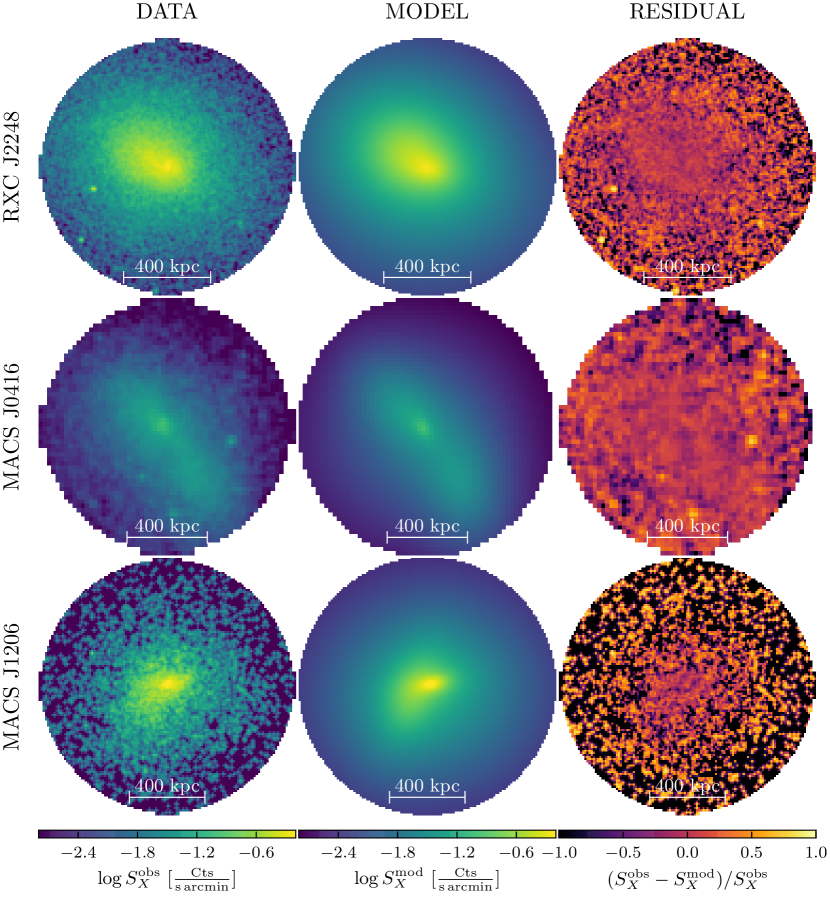
Figure 1 shows the X-ray surface brightness of the three clusters, one for each row. The first two columns show the logarithm of the observed data, $S^{\mathrm{obs}}_{X}$, and best-fit model, $S^{\mathrm{mod}}_{X}$, respectively. The images in the third column are the relative difference between the data and the model. Only circular apertures of radius $120\arcsec$ are shown, which correspond to those considered when fitting the cluster X-ray surface brightness. From these plots, it is clear that the complex geometry of the X-ray surface brightness requires multiple components to describe either individual subclusters, like in MACS J0416, or the asymmetry of the emission, like in MACS J1206. We note that in this work we provide an updated model of the hot intracluster gas in MACS J0416 presented in Bonamigo et al. (2017). While the previous spherical-component approximation provides a good fit to the data, the new elliptical model is favored by several model-selection criteria, such as the Akaike information criterion (AIC, Akaike, 1974) and Bayesian Information Criterion (BIC, Schwarz, 1978), and it is a more accurate representation the complex nature of this cluster.

Table 2: RXC J2248: Median values and confidence level (68%) uncertainties of the Three-Component dPIE Model of the X-Ray Surface Brightness. The center position refers to the BCG (R.A. $=$ 22:48:43.970 and decl. $=-$44:31:51.16).

	Comp. 1	Comp. 2	Comp. 3
$x_{0}$ ($\arcsec$)	$27^{+22}_{-21}$	$-18.2^{+0.6}_{-0.7}$	$0.2^{+0.4}_{-0.4}$
$y_{0}$ ($\arcsec$)	$-70^{+8}_{-15}$	$13.6^{+0.5}_{-0.5}$	$-1.2^{+0.3}_{-0.2}$
$\epsilon$	$0.71^{+0.12}_{-0.17}$	$0.13^{+0.01}_{-0.01}$	$0.34^{+0.02}_{-0.03}$
$\theta$ (degree)	$-163^{+8}_{-7}$	$-29^{+3}_{-2}$	$-15^{+2}_{-2}$
$R_{C}$ ($\arcsec$)	$188.6^{+0.1}_{-0.1}$	$36.0^{+0.5}_{-0.6}$	$14.6^{+0.3}_{-0.5}$
$R_{T}$ ($\arcsec$)	$189.1^{+0.1}_{-0.1}$	$360^{+50}_{-50}$	$359^{+4}_{-5}$
$\sigma_{0}$ (km s-1)	$440^{+20}_{-30}$	$539^{+6}_{-5}$	$308^{+7}_{-7}$

Table 3: MACS J0416: Median values and confidence level (68%) uncertainties of the Four-Component dPIE Model of the X-Ray Surface Brightness. The center position refers to the northeast BCG, G1 (R.A. $=$ 04:16:09.154 and decl. $=-$24:04:02.90).

	Comp. 1	Comp. 2	Comp. 3	Comp. 4
$x_{0}$ ($\arcsec$)	$-19.6^{+2.2}_{-1.4}$	$30.7^{+0.5}_{-0.7}$	$-2.3^{+0.1}_{-0.1}$	$-20.2^{+0.2}_{-0.1}$
$y_{0}$ ($\arcsec$)	$-13.2^{+1.4}_{-1.1}$	$-48.7^{+0.3}_{-0.2}$	$-1^{+0.1}_{-0.1}$	$14.6^{+0.6}_{-0.4}$
$\epsilon$	$0.09^{+0.05}_{-0.04}$	$0.41^{+0.03}_{-0.03}$	$0.42^{+0.04}_{-0.12}$	$0.39^{+0.03}_{-0.02}$
$\theta$ (degree)	$-160^{+10}_{-20}$	$-71^{+2}_{-3}$	$-52^{+5}_{-6}$	$-47^{+3}_{-2}$
$R_{C}$ ($\arcsec$)	$149.3^{+0.1}_{-0.1}$	$34.8^{+0.5}_{-0.8}$	$10.3^{+0.7}_{-0.8}$	$50.8^{+0.9}_{-0.9}$
$R_{T}$ ($\arcsec$)	$149.8^{+0.1}_{-0.1}$	$160^{+20}_{-10}$	$24.20^{+7}_{-5}$	$52.3^{+0.1}_{-0.1}$
$\sigma_{0}$ (km s-1)	$529^{+4}_{-2}$	$306^{+3}_{-4}$	$134^{+6}_{-5}$	$346^{+4}_{-6}$

Table 4: MACS J1206: Median values and confidence level (68%) uncertainties of the Three-Component dPIE Model of the X-Ray Surface Brightness. The center position refers to the BCG (R.A. $=$ 12:06:12.149 and decl. $=-$8:48:03.37).

	Comp. 1	Comp. 2	Comp. 3
$x_{0}$ ($\arcsec$)	$1.7^{+1.5}_{-0.9}$	$-13.9^{+1.5}_{-1.8}$	$3.3^{+0.7}_{-0.5}$
$y_{0}$ ($\arcsec$)	$-6.7^{+1.5}_{-1.3}$	$-7.6^{+1.4}_{-1.1}$	$2.1^{+0.4}_{-0.1}$
$\epsilon$	$0.13^{+0.03}_{-0.06}$	$0.50^{+0.07}_{-0.03}$	$0.55^{+0.06}_{-0.04}$
$\theta$ (degree)	$0^{+8}_{-10}$	$-111^{+4}_{-5}$	$-169^{+5}_{-2}$
$R_{C}$ ($\arcsec$)	$59^{+5}_{-2}$	$39^{+3}_{-2}$	$8.3^{+0.4}_{-0.8}$
$R_{T}$ ($\arcsec$)	$810^{+180}_{-400}$	$43.9^{+0.1}_{-0.1}$	$200^{+20}_{-110}$
$\sigma_{0}$ (km s-1)	$536^{+15}_{-6}$	$397^{+22}_{-8}$	$239^{+5}_{-13}$

The median values and confidence level (68%) uncertainties of the mass density parameters of the intracluster gas are presented in Tables 4, 4 and 4. The positions of the centers refer to the BCGs of the clusters (G1 for MACS J0416).

Table 5: RXC J2248: Median values and confidence level (CL) uncertainties for the strong-lensing model parameters. The center position refers to the BCG (R.A. $=$ 22:48:43.970 and decl. $=-$44:31:51.16). The angle $\theta_{h1}$ is measured counterclockwise from the West axis.

	Median	68% CL	95% CL	99.7% CL
$x_{h1}$ ($\arcsec$)	$1.8$	${}^{+0.3}_{-0.3}$	${}^{+0.6}_{-0.6}$	${}^{+1.0}_{-0.8}$
$y_{h1}$ ($\arcsec$)	$-1.0$	${}^{+0.2}_{-0.2}$	${}^{+0.4}_{-0.5}$	${}^{+0.6}_{-0.7}$
$\epsilon_{h1}$	$0.64$	${}^{+0.01}_{-0.01}$	${}^{+0.02}_{-0.01}$	${}^{+0.03}_{-0.02}$
$\theta_{h1}$ (degree)	$-38.7$	${}^{+0.3}_{-0.3}$	${}^{+0.5}_{-0.5}$	${}^{+0.7}_{-0.8}$
$R_{C,h1}$ ($\arcsec$)	$19.2$	${}^{+0.7}_{-0.6}$	${}^{+1.3}_{-1.3}$	${}^{+2.0}_{-1.9}$
$\sigma_{0,h1}$ (km s-1)	$1396$	${}^{+15}_{-17}$	${}^{+27}_{-35}$	${}^{+38}_{-53}$
$x_{h2}$ ($\arcsec$)	$-53.3$	${}^{+4.8}_{-6.0}$	${}^{+8.8}_{-12.8}$	${}^{+12.0}_{-21.4}$
$y_{h2}$ ($\arcsec$)	$27.1$	${}^{+2.8}_{-2.5}$	${}^{+6.3}_{-4.8}$	${}^{+10.9}_{-7.1}$
$\sigma_{0,h2}$ (km s-1)	$282$	${}^{+35}_{-31}$	${}^{+74}_{-60}$	${}^{+118}_{-86}$
$R_{T,g}$ ($\arcsec$)	$46.6$	${}^{+17.8}_{-13.8}$	${}^{+42.0}_{-25.1}$	${}^{+72.8}_{-33.7}$
$\sigma_{0,g}$ (km s-1)	$274$	${}^{+16}_{-16}$	${}^{+32}_{-33}$	${}^{+53}_{-51}$

Table 6: MACS J0416: Median values and confidence level (CL) uncertainties for the strong-lensing model parameters. The center position refers to the northeast BCG, G1 (R.A. $=$ 04:16:09.154 and decl. $=-$24:04:02.90). The angles $\theta_{h1}$ and $\theta_{h2}$ are measured counterclockwise from the West axis.

	Median	68% CL	95% CL	99.7% CL
$x_{h1}$ ($\arcsec$)	$-2.5$	${}^{+0.9}_{-0.8}$	${}^{+1.8}_{-1.4}$	${}^{+2.8}_{-1.9}$
$y_{h1}$ ($\arcsec$)	$1.8$	${}^{+0.5}_{-0.6}$	${}^{+0.9}_{-1.2}$	${}^{+1.3}_{-2.0}$
$\epsilon_{h1}$	$0.86$	${}^{+0.01}_{-0.01}$	${}^{+0.03}_{-0.03}$	${}^{+0.04}_{-0.06}$
$\theta_{h1}$ (degree)	$145.2$	${}^{+0.7}_{-0.9}$	${}^{+1.5}_{-1.9}$	${}^{+2.6}_{-2.8}$
$R_{C,h1}$ ($\arcsec$)	$6.7$	${}^{+0.7}_{-0.9}$	${}^{+1.4}_{-1.8}$	${}^{+2.1}_{-2.5}$
$\sigma_{0,h1}$ (km s-1)	$707$	${}^{+23}_{-23}$	${}^{+45}_{-51}$	${}^{+64}_{-83}$
$x_{h2}$ ($\arcsec$)	$19.9$	${}^{+0.3}_{-0.3}$	${}^{+0.8}_{-0.7}$	${}^{+1.6}_{-1.1}$
$y_{h2}$ ($\arcsec$)	$-37.0$	${}^{+0.6}_{-0.6}$	${}^{+1.3}_{-1.4}$	${}^{+1.9}_{-2.6}$
$\epsilon_{h2}$	$0.77$	${}^{+0.01}_{-0.01}$	${}^{+0.03}_{-0.03}$	${}^{+0.04}_{-0.05}$
$\theta_{h2}$ (degree)	$126.1$	${}^{+0.4}_{-0.4}$	${}^{+0.8}_{-0.9}$	${}^{+1.3}_{-1.3}$
$R_{C,h2}$ ($\arcsec$)	$12.5$	${}^{+0.6}_{-0.7}$	${}^{+1.2}_{-1.5}$	${}^{+1.9}_{-2.2}$
$\sigma_{0,h2}$ (km s-1)	$1064$	${}^{+16}_{-17}$	${}^{+31}_{-37}$	${}^{+49}_{-63}$
$x_{h3}$ ($\arcsec$)	$-34.4$	${}^{+0.9}_{-1.1}$	${}^{+1.9}_{-2.6}$	${}^{+2.7}_{-4.6}$
$y_{h3}$ ($\arcsec$)	$8.1$	${}^{+1.0}_{-0.7}$	${}^{+2.7}_{-1.4}$	${}^{+4.3}_{-2.0}$
$R_{C,h3}$ ($\arcsec$)	$4.4$	${}^{+2.4}_{-2.2}$	${}^{+4.8}_{-3.8}$	${}^{+7.4}_{-4.3}$
$\sigma_{0,h3}$ (km s-1)	$350$	${}^{+51}_{-48}$	${}^{+104}_{-84}$	${}^{+167}_{-107}$
$R_{T,g}$ ($\arcsec$)	$7.8$	${}^{+2.3}_{-1.5}$	${}^{+7.7}_{-3.4}$	${}^{+12.6}_{-4.5}$
$\sigma_{0,g}$ (km s-1)	$318$	${}^{+11}_{-74}$	${}^{+42}_{-101}$	${}^{+67}_{-121}$

Table 7: MACS J1206: Median values and confidence level (CL) uncertainties for the strong-lensing model parameters. The center position refers to the BCG (R.A. $=$ 12:06:12.149 and decl. $=-$8:48:03.37). The angles $\theta_{h1}$, $\theta_{h2}$, $\theta_{h3}$, and $\theta_{4}$ are measured counterclockwise from the West axis. The parameters $\gamma_{4}$ and $\theta_{4}$ are the shear and its angle.

	Median	68% CL	95% CL	99.7% CL
$x_{h1}$ ($\arcsec$)	$-0.9$	${}^{+0.4}_{-0.5}$	${}^{+0.8}_{-1.0}$	${}^{+1.2}_{-1.4}$
$y_{h1}$ ($\arcsec$)	$0.3$	${}^{+0.2}_{-0.3}$	${}^{+0.4}_{-0.5}$	${}^{+0.6}_{-0.8}$
$\epsilon_{h1}$	$0.69$	${}^{+0.03}_{-0.03}$	${}^{+0.05}_{-0.05}$	${}^{+0.08}_{-0.09}$
$\theta_{h1}$ (degree)	$19.7$	${}^{+0.9}_{-0.8}$	${}^{+1.8}_{-1.7}$	${}^{+2.7}_{-2.6}$
$R_{C,h1}$ ($\arcsec$)	$6.7$	${}^{+0.5}_{-0.5}$	${}^{+1.2}_{-1.1}$	${}^{+2.4}_{-1.6}$
$\sigma_{0,h1}$ (km s-1)	$968$	${}^{+41}_{-46}$	${}^{+95}_{-98}$	${}^{+182}_{-146}$
$x_{h2}$ ($\arcsec$)	$9.5$	${}^{+0.8}_{-0.7}$	${}^{+1.8}_{-1.4}$	${}^{+2.9}_{-2.1}$
$y_{h2}$ ($\arcsec$)	$4.0$	${}^{+0.7}_{-0.7}$	${}^{+1.5}_{-1.8}$	${}^{+2.4}_{-3.8}$
$\epsilon_{h2}$	$0.55$	${}^{+0.10}_{-0.11}$	${}^{+0.20}_{-0.21}$	${}^{+0.32}_{-0.30}$
$\theta_{h2}$ (degree)	$115.1$	${}^{+3.0}_{-2.4}$	${}^{+6.5}_{-4.5}$	${}^{+10.3}_{-6.4}$
$R_{C,h2}$ ($\arcsec$)	$13.9$	${}^{+1.5}_{-1.1}$	${}^{+3.4}_{-2.0}$	${}^{+6.1}_{-2.8}$
$\sigma_{0,h2}$ (km s-1)	$758$	${}^{+37}_{-36}$	${}^{+79}_{-79}$	${}^{+123}_{-147}$
$x_{h3}$ ($\arcsec$)	$-28.6$	${}^{+1.4}_{-1.7}$	${}^{+2.8}_{-5.1}$	${}^{+4.2}_{-26.2}$
$y_{h3}$ ($\arcsec$)	$-6.7$	${}^{+0.9}_{-0.8}$	${}^{+2.8}_{-1.6}$	${}^{+7.6}_{-2.5}$
$\epsilon_{h3}$	$0.35$	${}^{+0.06}_{-0.06}$	${}^{+0.13}_{-0.13}$	${}^{+0.19}_{-0.20}$
$\theta_{h3}$ (degree)	$-25.4$	${}^{+10.2}_{-11.6}$	${}^{+18.0}_{-22.5}$	${}^{+24.0}_{-33.7}$
$R_{C,h3}$ ($\arcsec$)	$12.3$	${}^{+2.3}_{-2.1}$	${}^{+5.1}_{-4.0}$	${}^{+14.1}_{-6.1}$
$\sigma_{0,h3}$ (km s-1)	$600$	${}^{+45}_{-41}$	${}^{+97}_{-84}$	${}^{+157}_{-159}$
$\gamma_{4}$	$0.11$	${}^{+0.01}_{-0.01}$	${}^{+0.02}_{-0.02}$	${}^{+0.03}_{-0.03}$
$\theta_{4}$ (degree)	$101.5$	${}^{+1.5}_{-1.4}$	${}^{+3.0}_{-3.4}$	${}^{+4.8}_{-6.8}$
$R_{T,g}$ ($\arcsec$)	$3.6$	${}^{+0.9}_{-0.7}$	${}^{+1.9}_{-1.4}$	${}^{+3.2}_{-2.0}$
$\sigma_{0,g}$ (km s-1)	$353$	${}^{+24}_{-21}$	${}^{+53}_{-40}$	${}^{+93}_{-57}$

The next step in the analysis is to include these hot gas models as fixed mass components in the strong lensing analysis. We use a first optimization of the lensing model of each cluster to derive new values for the error in the positions of the multiple images. These are $0\arcsec.46$, $0\arcsec.57$ and $0\arcsec.35$, for RXC J2248, MACS J0416 and MACS J1206, respectively. The subsequent best-fit models have values of the minimum-$\chi^{2}$ of $59.71$ (59 d.o.f), $111.0$ (110 d.o.f) and $90.9$ (88 d.o.f); the corresponding values of the rms of the multiple-image position offsets are $0\arcsec.48$, $0\arcsec.59$ and $0\arcsec.45$ (median values $0\arcsec.37$, $0\arcsec.40$ and $0\arcsec.36$). Tables 5, 6 and 7 contain the inferred values of the mass model parameters. Here, we quote the median values and the $68\%$, $95\%$ and $99.7\%$ confidence level (CL) intervals.

Figure 2: Surface mass density of RXC J2248 (top row), MACS J0416 (middle row) and MACS J1206 (bottom row) overlaid on color-composite HST WCF3+ACS images. White, blue and red isodensity contours (left panel) correspond to total, diffuse DM and hot intracluster gas, respectively. The total and diffuse DM contours are drawn at $3.5$, $7.2$, $15$ and $30$ in units of $10^{-4}$ M${}_{\odot}/$kpc²; while the hot gas contours are drawn at $0.65$, $1.0$, $1.6$ and $2.5$ in units of $10^{-4}$ M${}_{\odot}/$kpc². The right panel is a zoom-in of the central region of each cluster. The green plus sign indicates the position of the BCG and has a total width of $2\arcsec$. Blue contours (right panel) show the $1\sigma$, $2\sigma$ and $3\sigma$ confidence levels of the diffuse DM component density peak.

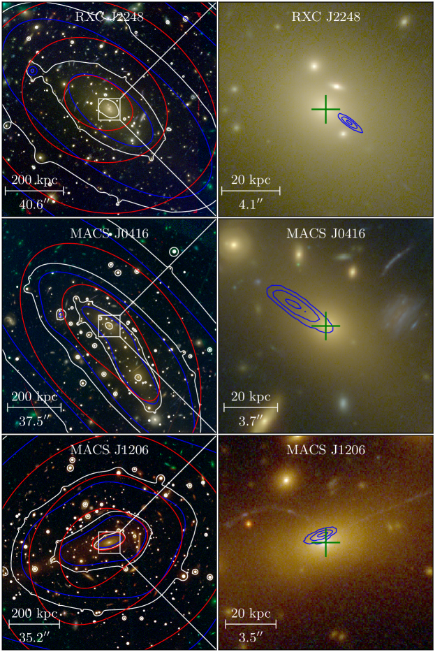
The surface mass densities of the different cluster components are shown in Figure 2 (left panel), where they are represented as iso-contours overlaid on color-composite HST WCF3/ACS images of the clusters. The total (white) and DM (blue) isodensity contours are drawn at $3.5$, $7.2$, $15$ and $30$ in units of $10^{-4}$ M${}_{\odot}/$kpc²; while the gas (red) isodensity contours are drawn at $0.65$, $1.0$, $1.6$ and $2.5$ in units of $10^{-4}$ M${}_{\odot}/$kpc². The right panel of Figure 2 shows a zoom-in of the central region of the images on the left. The positions of the BCGs are shown with green plus signs, that are $2\arcsec$ of width. The blue contours in the right panel show the position of the diffuse DM component density peak with $1\sigma$, $2\sigma$ and $3\sigma$ confidence levels. From these plots, the need for a full component separation is clear: the DM and hot-gas mass distributions have different shapes and centers, due to their intrinsically different physical properties. For example, while the DM component in RXC J2248 is roughly centered on the BCG, the hot-gas mass distribution is skewed towards northeast. In MACS J1206, this latter component is elongated towards the southeast region of the cluster, creating a twist in the iso-density contours; such feature is not present in the DM mass distribution, which, however, tends to be fairly lopsided. In all clusters, especially in RXC J2248, the hot-gas component is rounder than the DM one; in MACS J0416, this happens a-symmetrically, with the northeast region being rounder than the southeast one. Moreover, with the exception of RXC J2248, we find that the peaks of the density of the diffuse DM components are consistent, within 3$\sigma$, with the positions of the BCGs. Indeed, the distances between the BCGs and the DM component density peaks are $(9.3^{+1.7}_{-1.7})$, $(13.8^{+4.7}_{-5.3})$, and $(3.9^{+1.0}_{-0.8})$ kpc, for RXC J2248, MACS J0416 and MACS J1206, respectively. We note that RXC J2248 is described by the simplest DM mass model and that the DM component seems to counterbalance the a-symmetric hot gas component, which is skewed in the opposite direction.

Figure 3: Radial profiles of the surface mass density (left panel) and cumulative projected mass (right panel) for the different components of RXC J2248 (first row), MACS J0416 (second row) and MACS J1206 (third row). Black, blue, red, and green curves correspond to total, diffuse DM, hot gas and cluster members, respectively. Thin lines show a subsample of the posterior distribution, while solid and dashed lines show the median and $16^{\text{th}}\,$-$\,84^{\text{th}}$ percentiles. Reference logarithmic slopes are also indicated.

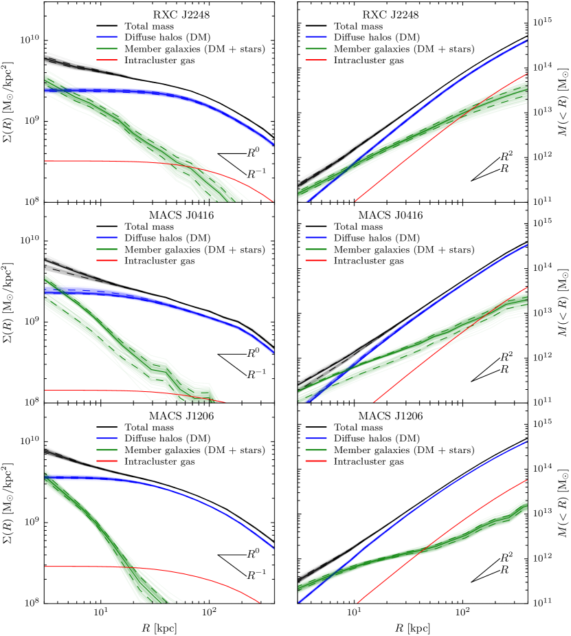
From the previous maps, we obtain the radial profiles shown in Figure 3. Left and right panels contain, respectively, the surface mass density and cumulative projected mass profiles; each color corresponds to a different mass component: cluster members (green), hot intracluster gas (red), DM (blue), and total (black). Thin lines represent a subsample of the models extracted from the sampling of the posterior distribution, while solid and dashed lines show their median and $16^{\text{th}}\,$-$\,84^{\text{th}}$ percentiles, respectively.

5 Discussion

In order to compare the results of the different clusters in a consistent way, we decide to rescale the values of their masses, surface mass densities, and radii. To do this, we use the values of the mass $M_{200\textrm{c}}$ and of the corresponding radius $R_{200\textrm{c}}$, derived by Umetsu et al. (2014) via a weak-lensing shear-and-magnification analysis (see Table 1). Respectively, for RXC J2248, MACS J0416 and MACS J1206 the values of $M_{200\textrm{c}}$ are $(2.03\pm 0.67)$, $(1.04\pm 0.22)$ and $(1.59\pm 0.36)\times 10^{15}$ M_⊙. In passing, we mention that these values are consistent, given the errors, with those obtained by Biviano et al. (2013) and Balestra et al. (2016) from the dynamical analyses of MACS J1206 and MACS J0416, respectively. These masses correspond to values of $R_{200\textrm{c}}$ of $(2.32\pm 0.26)$, $(1.82\pm 0.13)$ and $(2.06\pm 0.16)$ Mpc. In our analysis, we include the error of the weak-lensing measurement of a cluster total mass, $M_{200\textrm{c}}$, and radius, $R_{200\textrm{c}}$, by considering that they are described by Gaussian distributions.

Figure 4: Normalized radial profiles of the total surface mass density (left panel) and cumulative projected mass (right panel) of RXC J2248 (blue), MACS J0416 (red) and MACS J1206 (green). Thin lines show a subsample of the posterior distribution, while solid and dashed lines show the mean and standard deviation.

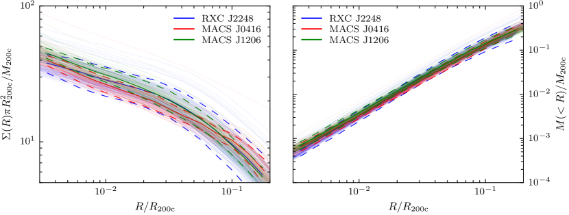
Once rescaled, the total surface mass density and cumulative projected mass profiles show a very uniform behavior, as it can be seen on the left and right panels of Figure 4, respectively. Thin lines represent a subsample of the models extracted from the sampling, while solid and dashed lines show the mean and standard deviation. In these and following figures, we have identified each cluster with a different color: blue for RXC J2248, red for MACS J0416 and green for MACS J1206. Even though these measurements are dominated by the errors on the total mass and radius from the weak-lensing analysis, the differences between the three clusters are small, both in terms of density and enclosed mass, suggesting the existence of a homologous mass profile. In Appendix C, we fit these profiles with Navarro-Frenk-White profiles (Navarro et al., 1997) and discuss the caveats of claiming “universality” of mass profiles that are fitted in projection. It should be noted that this remarkably good agreement between the rescaled mass profiles was not expected a priori: the values of $M_{200\textrm{c}}$ have been measured at much larger scales ($R\sim R_{200\textrm{c}}$) through weak lensing (Umetsu et al., 2014), while the current analysis is restricted only to the cores of the clusters ($R<0.2R_{200\textrm{c}}$). Previous works (Biviano et al., 2013; Grillo et al., 2015; Balestra et al., 2016; Caminha et al., 2017b) have shown though that in these clusters with high-quality data the results of different mass diagnostics, where they overlap, agree very well.

Using the surface mass densities of the different cluster components (from Figure 2), we can create maps of the diffuse DM and hot gas over total mass fractions.

Figure 5: Maps of the diffuse DM (left column) and hot intracluster gas (right column) over total mass fractions of RXC J2248 (first row), MACS J0416 (second row) and MACS J1206 (third row).

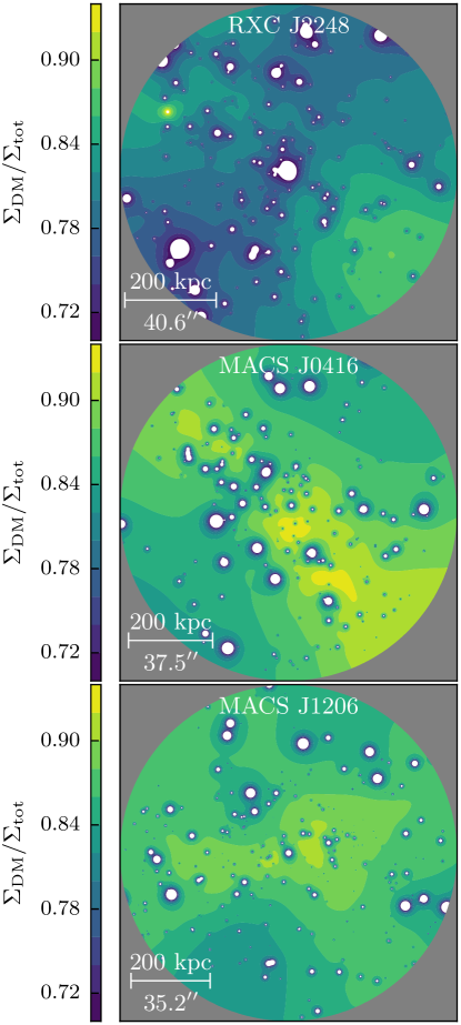
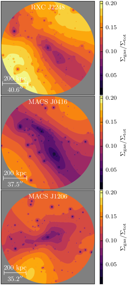
These are shown, respectively, on the left and right panel of Figure 5. While the galaxy clusters MACS J0416 and MACS J1206 have comparable fractions of DM, with similar trend with the radial distance from the center, RXC J2248 has a lower DM fraction and a much steeper radial dependence. Moreover, the alignment of the DM fraction iso-contours seems to be perpendicular to the orientation of the cluster. This apparent misalignment is due to a combination of multiple factors. First, the difference in shape between the DM and hot gas mass distributions causes the DM to become less dominant along the direction perpendicular to its mass distribution major axis; although less pronounced, this effect can also be seen in MACS J0416. Secondly, the offset between the gas and DM components causes the southeast region to have less hot gas and therefore a larger DM mass fraction. Moreover, these effects are increased by the larger truncation radii of the cluster member galaxies, $R_{T,g}$, that extend their influence in the total mass budget. On the other hand, the hot gas over total mass fraction maps are more consistent between the clusters, with their centers having lower fractions than the outskirts. However, the central regions of MACS J0416 show a low value, which is consistent with the cluster merging nature: the turbulence of the merger is heating the gas, preventing it to fall to the center. In contrast, RXC J2248 and MACS J1206 have a cool-core, that results in the higher gas fraction shown on the left panel of Figure 5.

Figure 6: Ratios of the cumulative projected hot gas and total mass for RXC J2248 (blue), MACS J0416 (red) and MACS J1206 (green). Thin lines show a subsample of the posterior distribution, while solid and dashed lines show the mean and standard deviation.

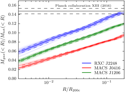
The same trend can be seen in Figure 6, where we show the ratios of the cumulative projected hot gas and total mass. As before, we rescale the radial distance by $R_{200\textrm{c}}$, to remove the dependence on the cluster mass, and include the corresponding uncertainties which dominate the errors shown in Figure 6. Colors and lines are defined as in Figure 4. The horizontal black solid and dashed lines show the cosmological baryon fraction with errors measured by the Planck satellite (Planck collaboration XIII 2016). This is the quantity of cosmological interest, which can be obtained by adding the fraction of stellar mass to that of the hot gas measured in this paper, as done by Annunziatella et al. (2017) in MACS J0416. We postpone to future works the measurement of the stellar mass component of RXC J2248 and MACS J1206. Noticeably, we are able to measure the hot gas fraction with very high precision, (less than $1\%$ before rescaling), thanks to the small uncertainties on the cluster total mass derived from our high-precision strong lensing models.

Finally, expanding the analysis by Grillo et al. (2015) and Munari et al. (2016), we look at the substructure statistics in the three clusters, traced by their member galaxies. We compare our measurements, derived from the new strong lensing model (Section 2.2), to those presented by Grillo et al. (2015), both on the observed data of MACS J0416 and the simulated halos. In order to increase the statistics, we consider here simulated ($N$-body) halos that have $M_{200c}$ values larger than $9\times 10^{14}M_{\odot}$ from four snapshots, at the following redshifts: $0.25$, $0.28$, $0.46$ and $0.51$. In all clusters, we select only those galaxies, or sub-halos, that have a circular velocity value $v_{c}=\sqrt{2}\sigma_{0}$ larger than $90$ km s^-1 and that are located within a projected distance of $0.16\times R_{200\mathrm{c}}$ from the cluster centers. Compared to the previous studies, we change these velocity and projected distance limits in order to better compare clusters with different masses and to avoid the mass resolution limit that would otherwise contaminate the results at the low circular velocity end for the simulated sub-halos. We refer to the original papers for any other details on the strong lensing model and simulated data.

Figure 7: Radial profiles of the number density and circular velocity distributions of the member galaxies for RXC J2248 (blue), MACS J0416 (red) and MACS J1206 (green). Only galaxies within a circular aperture of $0.16\times R_{200\mathrm{c}}$ and with circular velocity larger than $90$ km s^-1 are considered. Points and error bars show the median and $16^{\text{th}}\,$-$\,84^{\text{th}}$ percentiles, respectively. Red histograms are the values derived from the model of MACS J0416 by Grillo et al. (2015), where a slightly different value for the center of the cluster was adopted.

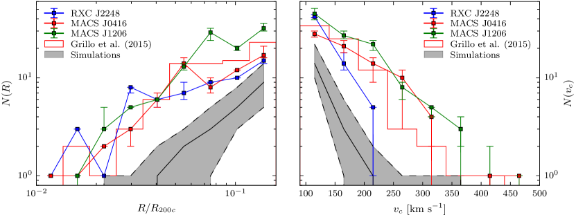
Then, we compute the galaxy radial number distribution and circular velocity distribution. We show them, respectively, in the left and right panels of Figure 7.

Figure 8: Circular velocity function of the member galaxies for RXC J2248 (blue), MACS J0416 (red) and MACS J1206 (green). Only galaxies within a circular aperture of $0.16\times R_{200\mathrm{c}}$ and with a circular velocity larger than $90$ km s^-1 are considered. Points and error bars show the median and $16^{\text{th}}\,$-$\,84^{\text{th}}$ percentiles, respectively.

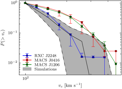
Moreover, in Figure 8, we show the circular velocity function of the member galaxies, i.e. the fraction of member galaxies with circular velocity larger than the considered value. In both plots, the points with error bars mark the median and $16^{\text{th}}\,$-$\,84^{\text{th}}$ percentiles, computed from a sample of models extracted from the MCMC sampling. The gray-shaded areas represent the values obtained from numerical simulations, as presented by Grillo et al. (2015). In Figure 7, we also show the observed data from Grillo et al. (2015). The color scheme is the same as in the previous plots. Interestingly, the circular velocity function of the cluster members of MACS J1206 is more similar to that of MACS J0416, a merging cluster, than to that of RXC J2248, a relaxed cluster. In their work, Grillo et al. (2015) noticed how the number of massive substructures ($v_{c}>100$ km s^-1) is underestimated in numerical simulations, even when baryonic effects are included (Munari et al., 2016). Similarly, we find that both in terms of radial and velocity distributions, the results presented in this work are consistent with those by Grillo et al. (2015), i.e. in tension with the predictions of numerical simulations, and partially at odds with those by Natarajan et al. (2017). Only the circular velocity function of RXC J2248 seems to be within the intrinsic scatter of the simulated data; however, in the observed cluster the number of sub-halos with a given circular velocity is still a factor of approximately three larger than what found in simulations. These differences can not be solved by invoking possible misidentifications of cluster members, as our extensive spectroscopy and 12-band CLASH photometry lead to highly pure samples (i.e., very few false positives) and the vast majority of the high-velocity cluster members are confirmed spectroscopically (see Fig. 4 in Caminha et al., 2017a).

6 Conclusions

Thanks to the very high quality of the multi-wavelength data available, we have been able to separate the collisional and collisionless mass components in the galaxy clusters RXC J2248.7$-$4431, MACS J0416.1$-$2403, and MACS J1206.2$-$0847 at $z\approx 0.4$. Two of them, RXC J2248 and MACS J0416, are part of the HFF sample (Lotz et al., 2017) and all three have been observed with both the VIMOS (CLASH-VLT program; Rosati et al., 2014) and the MUSE (archive observations) instruments at the VLT. Following the method presented by Bonamigo et al. (2017), we have modeled the hot gas mass by fitting the X-ray surface brightness from deep Chandra observations of the clusters. Then, we have introduced this mass term in the strong lensing analysis as a fixed component.

The main results of the work can be summarized as follows:

1. We have provided 2D models of the hot intracluster gas mass density of these three clusters (updating that of MACS J0416) that are consistent with a well tested and independent approach (Ettori et al., 2013) and that can be easily included in different gravitational lensing softwares.

2. With the decoupling of the hot gas from the other cluster mass components, we have improved previous strong-lensing models to describe more accurately the different contributions to the total mass budget of the clusters. Due to their different physical nature, the cluster hot gas and DM halo components exhibit different properties, seen both in their surface mass density maps and cumulative radial mass profiles.

3. The isolation of the diffuse DM component has allowed us to measure with high accuracy the absence of a significant offset between the diffuse DM density peaks and the positions of the BCGs, which is a test for models of self-interacting dark matter.

4. By rescaling the radial profiles of the cluster projected mass with the values of $R_{200\textrm{c}}$ and $M_{200\textrm{c}}$, we have shown that these clusters manifest an almost homologous structure, despite their significantly different relaxation status.

5. By exploiting the small statistical uncertainties on the cluster total mass derived from our strong-lensing analysis, we have measured the hot gas over total mass fraction throughout the core of the clusters with unprecedented precision (less than $1\%$). A remarkable advantage of the adopted approach is the possibility of investigating spatially resolved maps of the gas fraction, in addition to the traditional radial profiles.

6. Finally, we have confirmed the findings by Grillo et al. (2015) and Munari et al. (2016) that current $N$-body simulations under-predict the number of massive sub-halos ($v_{c}>90$ km s^-1) in the cores of massive clusters. This discrepancy is visible in all three clusters of our sample.

In this paper we have shown the advantages of an accurate multi-wavelength study of a well selected sample of clusters with high-quality data. Being able to extend the sample to even more clusters and comparing with the outcomes of cosmological simulations will allow to tackle some of the still open questions about the nature of DM and the internal structure of galaxy clusters. The importance of detailed and accurate studies of galaxy clusters is clear. In this era of large all-sky surveys, the information gained from vast samples of galaxy clusters rely on the accuracy of the adopted priors and models. Only by testing these assumptions on a smaller, well-understood sample it is possible to push forward our knowledge of DM and the other components of the Universe.

Appendix A Alternative hot gas mass models

When fitting the X-ray surface brightness, we model the cluster hot gas mass density distributions with either two or three components (three and four for MACS J0416), with both spherical and elliptical symmetry. The selection of the final best-fitting model is done by considering the Akaike information criterion (AIC, Akaike, 1974) and the Bayesian Information Criterion (BIC, Schwarz, 1978). As here we are mainly interested in the projected mass profiles of the clusters, we compare our results with independent measurements of the cumulative projected hot gas mass profiles of RXC J2248, MACS J0416, and MACS J1206.

Figure 9: Cumulative projected hot gas mass profiles of RXC J2248, MACS J0416 and MACS J1206, respectively, on the left, center and right panel. Dashed and solid lines show, the spherical- and elliptical-component models, respectively. Black, blue and red lines refer to models with two, three and four components. The gray areas show the $1$-sigma confidence regions of the mass profile obtained through a geometrical deprojection.

In Fig. 9, the gray areas show the $1$-sigma confidence regions of these mass profiles, while the dashed and solid lines show, respectively, the spherical- and elliptical-component models tested in this work (based on Bonamigo et al., 2017). Different colors represent models with different numbers of components, as indicated on the legends. The model used as comparison has been recovered through the geometrical deprojection (see, e.g., Ettori et al., 2013, and references therein) of the azimuthally averaged surface brightness profile that considers the entire X-ray emission of the cluster. The striking agreement with this different and independent method corroborates the accuracy of our measurements, especially in the regions of interest in the lensing analysis, i.e. $R<400$ kpc.

Appendix B Effect of the intrinsic variance of the $\chi^{2}$ distribution

As any other distribution, the $\chi^{2}$ distribution has an intrinsic variance that is a function of the model degrees of freedom. Because of this, even a perfect model is not guaranteed to have a value of the $\chi^{2}$ equal to the number of the degrees of freedom (Andrae et al., 2010). Therefore, when we require the best-fit model to have a $\chi^{2}$ value approximately equal to the number of degrees of freedom, we introduce a systematic error, that propagates into the uncertainties on the mass-component parameter distributions and on the mass and density radial profiles.

To better quantify this effect, we consider the value of the $0.13$ percentile ($99.7\%$ confidence level) of the $\chi^{2}$ distribution for our best-fit strong-lensing model of RXC J2248. This gives a conservative model that can be considered as an upper limit on the errors of the mass models presented in this paper. Given the $59$ degrees of freedom for RXC J2248, the $0.13$-percentile of the corresponding $\chi^{2}$ distribution is $31.7$. Therefore, to investigate this more conservative model, we increase the uncertainty on the image positions to $0^{\prime\prime}.66$, in order to get a minimum chi-square value of approximately 32, while in the main-text model the error is $0^{\prime\prime}.48$.

Figure 10: Radial profiles of the surface mass density (left panel) and cumulative projected mass (right panel) for the total (black) and dark-matter component (blue) of RXC J2248. The areas show values at the 3$\sigma$ confidence level. Darker and lighter refer to values of the minimum $\chi^{2}$ of approximately $59$ (reference model in this work) and $32$, respectively.

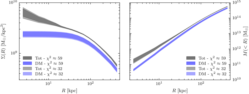
We then use the same procedure presented above to compute the surface mass density and cumulative projected mass radial profiles and show them, respectively, on the left and right panel of Figure 10. The filled areas represent the $3\sigma$ uncertainties on the radial profiles of the main-text (darker colors) and conservative (lighter colors) models, respectively. Black and blue areas show the total and DM-only component.

We remark that the $3\sigma$ confidence level values of the profiles shown in Figure 10 for the two different models are very similar. The results of this test thus suggest that the variance of the $\chi^{2}$ distribution does not affect significantly the final errors on the values of the parameters and of the derived quantities of a model.

Appendix C On the homologous projected profiles

As noted in Section 5, the rescaled surface density and cumulative projected mass profiles of the three clusters are very similar, suggesting the existence of a homologous mass profile. Indeed, DM-only numerical simulations have shown that the averaged mass profile of virialized halos is well described by a universal profile, the so-called Navarro-Frenk-White profile (NFW; Navarro et al., 1997). We use a NFW profile to fit, separately, both the surface mass density and the cumulative projected mass profiles estimated in our strong lensing analyses.

Figure 11: Radial profiles of the total surface mass density (left panel) and cumulative projected mass (right panel) of RXC J2248 (blue), MACS J0416 (red) and MACS J1206 (green). Data points with error bars show the fitted data, measured from the strong lensing analysis. Solid lines represent the best-fit NFW profiles to the data.

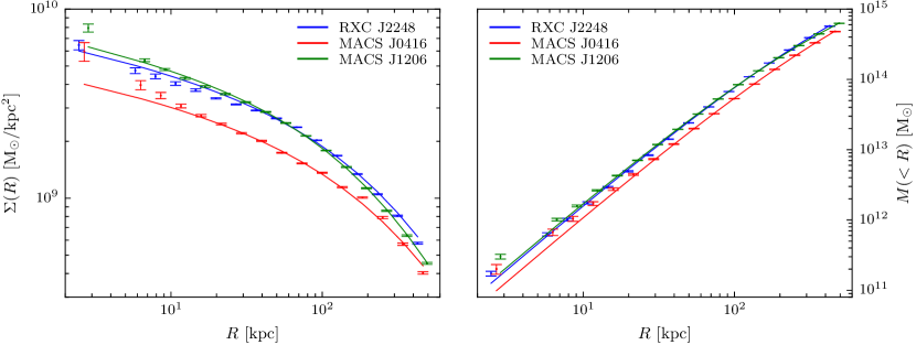
The best-fitting profiles obtained from the optimized values are shown in Fig. 11 as solid lines. Points with error bars show the mean and standard deviation of the measured surface mass density (left panel) and cumulative projected mass (right panel) that have been fitted. With the exception of the innermost regions, dominated by the BCGs, a NFW profile provides a good fit to the data, as shown in Umetsu et al. (2014) for the CLASH cluster sample. We remark though that the data points are obtained from the combination of multiple components, described by different (cored) isothermal mass profiles, which are favored over the NFW profiles by the strong lensing analyses, as shown in Grillo et al. (2015) and Caminha et al. (2017b) for MACS J0416 and MACS J1206, respectively. This suggests that other one-component models, with a varying radial slope, might also provide good fits to the reconstructed profiles of the clusters in their cores, when they are considered in projection. We believe that the best way to distinguish among the different models is to use the chi-square statistics directly on the difference between the observed and model-predicted positions of the multiple images and that a good fit on the reconstructed projected quantities of a complex astrophysical object might not be enough to state the definite success of a particular model.

References

- Abell et al. (1989) Abell, G. O., Corwin, Jr., H. G., & Olowin, R. P. 1989, ApJS, 70, 1
- Acebron et al. (2017) Acebron, A., Jullo, E., Limousin, M., et al. 2017, MNRAS, 470, 1809
- Akaike (1974) Akaike, H. 1974, IEEE Transactions on Automatic Control, 19, 716
- Allen et al. (2008) Allen, S. W., Rapetti, D. A., Schmidt, R. W., et al. 2008, MNRAS, 383, 879
- Andrae et al. (2010) Andrae, R., Schulze-Hartung, T., & Melchior, P. 2010, ArXiv e-prints, arXiv:1012.3754
- Annunziatella et al. (2017) Annunziatella, M., Bonamigo, M., Grillo, C., et al. 2017, ArXiv e-prints, arXiv:1711.02109
- Bacon et al. (2012) Bacon, R., Accardo, M., Adjali, L., et al. 2012, The Messenger, 147, 4
- Balestra et al. (2013) Balestra, I., Vanzella, E., Rosati, P., et al. 2013, A&A, 559, L9
- Balestra et al. (2016) Balestra, I., Mercurio, A., Sartoris, B., et al. 2016, ApJS, 224, 33
- Bender et al. (1992) Bender, R., Burstein, D., & Faber, S. M. 1992, ApJ, 399, 462
- Biviano et al. (2013) Biviano, A., Rosati, P., Balestra, I., et al. 2013, A&A, 558, A1
- Böhringer et al. (2001) Böhringer, H., Schuecker, P., Guzzo, L., et al. 2001, A&A, 369, 826
- Bonamigo et al. (2017) Bonamigo, M., Grillo, C., Ettori, S., et al. 2017, ApJ, 842, 132
- Caminha et al. (2016) Caminha, G. B., Grillo, C., Rosati, P., et al. 2016, A&A, 587, A80
- Caminha et al. (2017a) —. 2017a, A&A, 600, A90
- Caminha et al. (2017b) —. 2017b, A&A, 607, A93
- Chirivì et al. (2017) Chirivì, G., Suyu, S. H., Grillo, C., et al. 2017, ArXiv e-prints, arXiv:1706.07815
- Clowe et al. (2006) Clowe, D., Bradač, M., Gonzalez, A. H., et al. 2006, ApJ, 648, L109
- Donahue et al. (2014) Donahue, M., Voit, G. M., Mahdavi, A., et al. 2014, ApJ, 794, 136
- Elíasdóttir et al. (2007) Elíasdóttir, Á., Limousin, M., Richard, J., et al. 2007, ArXiv e-prints, arXiv:0710.5636
- Ettori (2000) Ettori, S. 2000, MNRAS, 311, 313
- Ettori et al. (2013) Ettori, S., Donnarumma, A., Pointecouteau, E., et al. 2013, Space Sci. Rev., 177, 119
- Ettori et al. (2003) Ettori, S., Tozzi, P., & Rosati, P. 2003, A&A, 398, 879
- Evrard (1997) Evrard, A. E. 1997, MNRAS, 292, 289
- Faber et al. (1987) Faber, S. M., Dressler, A., Davies, R. L., Burstein, D., & Lynden-Bell, D. 1987, in Nearly Normal Galaxies. From the Planck Time to the Present, ed. S. M. Faber, 175–183
- Firmani et al. (2000) Firmani, C., D’Onghia, E., Avila-Reese, V., Chincarini, G., & Hernández, X. 2000, MNRAS, 315, L29
- Grillo et al. (2015) Grillo, C., Suyu, S. H., Rosati, P., et al. 2015, ApJ, 800, 38
- Grillo et al. (2016) Grillo, C., Karman, W., Suyu, S. H., et al. 2016, ApJ, 822, 78
- Jullo et al. (2007) Jullo, E., Kneib, J.-P., Limousin, M., et al. 2007, New Journal of Physics, 9, 447
- Karman et al. (2017) Karman, W., Caputi, K. I., Caminha, G. B., et al. 2017, A&A, 599, A28
- Kassiola & Kovner (1993) Kassiola, A., & Kovner, I. 1993, ApJ, 417, 450
- Kawamata et al. (2017) Kawamata, R., Ishigaki, M., Shimasaku, K., et al. 2017, ArXiv e-prints, arXiv:1710.07301
- Lagattuta et al. (2017) Lagattuta, D. J., Richard, J., Clément, B., et al. 2017, MNRAS, 469, 3946
- Lotz et al. (2017) Lotz, J. M., Koekemoer, A., Coe, D., et al. 2017, ApJ, 837, 97
- Macciò et al. (2012) Macciò, A. V., Paduroiu, S., Anderhalden, D., Schneider, A., & Moore, B. 2012, MNRAS, 424, 1105
- Mahler et al. (2018) Mahler, G., Richard, J., Clément, B., et al. 2018, MNRAS, 473, 663
- Mann & Ebeling (2012) Mann, A. W., & Ebeling, H. 2012, MNRAS, 420, 2120
- Monna et al. (2017) Monna, A., Seitz, S., Balestra, I., et al. 2017, MNRAS, arXiv:1605.08784
- Morandi et al. (2012) Morandi, A., Limousin, M., Sayers, J., et al. 2012, MNRAS, 425, 2069
- Munari et al. (2016) Munari, E., Grillo, C., De Lucia, G., et al. 2016, ApJ, 827, L5
- Natarajan et al. (2017) Natarajan, P., Chadayammuri, U., Jauzac, M., et al. 2017, MNRAS, 468, 1962
- Navarro et al. (1997) Navarro, J. F., Frenk, C. S., & White, S. D. M. 1997, ApJ, 490, 493
- Ogrean et al. (2016) Ogrean, G. A., van Weeren, R. J., Jones, C., et al. 2016, ApJ, 819, 113
- Planck Collaboration et al. (2016) Planck Collaboration, Ade, P. A. R., Aghanim, N., et al. 2016, A&A, 594, A13
- Planelles et al. (2013) Planelles, S., Borgani, S., Dolag, K., et al. 2013, MNRAS, 431, 1487
- Postman et al. (2012) Postman, M., Coe, D., Benítez, N., et al. 2012, ApJS, 199, 25
- Richard et al. (2015) Richard, J., Patricio, V., Martinez, J., et al. 2015, MNRAS, 446, L16
- Rosati et al. (2014) Rosati, P., Balestra, I., Grillo, C., et al. 2014, The Messenger, 158, 48
- Rumsey et al. (2016) Rumsey, C., Olamaie, M., Perrott, Y. C., et al. 2016, MNRAS, 460, 569
- Salmon et al. (2017) Salmon, B., Coe, D., Bradley, L., et al. 2017, ArXiv e-prints, arXiv:1710.08930
- Schwarz (1978) Schwarz, G. 1978, Ann. Statist., 6, 461
- Sereno et al. (2017) Sereno, M., Ettori, S., Meneghetti, M., et al. 2017, ArXiv e-prints, arXiv:1702.00795
- Spergel & Steinhardt (2000) Spergel, D. N., & Steinhardt, P. J. 2000, Physical Review Letters, 84, 3760
- Suyu & Halkola (2010) Suyu, S. H., & Halkola, A. 2010, A&A, 524, A94
- Umetsu et al. (2014) Umetsu, K., Medezinski, E., Nonino, M., et al. 2014, ApJ, 795, 163
- Umetsu et al. (2015) Umetsu, K., Sereno, M., Medezinski, E., et al. 2015, ApJ, 806, 207
- van Weeren et al. (2017) van Weeren, R. J., Ogrean, G. A., Jones, C., et al. 2017, ArXiv e-prints, arXiv:1701.04096
- Vogelsberger et al. (2012) Vogelsberger, M., Zavala, J., & Loeb, A. 2012, MNRAS, 423, 3740
- Wechsler et al. (2002) Wechsler, R. H., Bullock, J. S., Primack, J. R., Kravtsov, A. V., & Dekel, A. 2002, ApJ, 568, 52
- White et al. (1993) White, S. D. M., Navarro, J. F., Evrard, A. E., & Frenk, C. S. 1993, Nature, 366, 429
- Zhao et al. (2003) Zhao, D. H., Mo, H. J., Jing, Y. P., & Börner, G. 2003, MNRAS, 339, 12
- Zitrin et al. (2012) Zitrin, A., Rosati, P., Nonino, M., et al. 2012, ApJ, 749, 97