Dep. of Mathematics and Computer Science, TU Eindhoven, The Netherlands
[k.a.buchin|t.a.e.ophelders|b.speckmann]@tue.nl
The authors are supported by the Netherlands Organisation for Scientific Research (NWO) under project no. 612.001.207 (Kevin Buchin) and no. 639.023.208 (Tim Ophelders and Bettina Speckmann).
\CopyrightKevin Buchin and Tim Ophelders and Bettina Speckmann
\ArticleNo0
\hideLIPIcs
SETH Says: Weak Fréchet Distance is Faster, but only if it is Continuous and in One Dimension
Abstract.
We show by reduction from the Orthogonal Vectors problem that algorithms with strongly subquadratic running time cannot approximate the Fréchet distance between curves better than a factor unless SETH fails. We show that similar reductions cannot achieve a lower bound with a factor better than . Our lower bound holds for the continuous, the discrete, and the weak discrete Fréchet distance even for curves in one dimension. Interestingly, the continuous weak Fréchet distance behaves differently. Our lower bound still holds for curves in two dimensions and higher. However, for curves in one dimension, we provide an exact algorithm to compute the weak Fréchet distance in linear time.
Key words and phrases:
SETH, Orthogonal Vectors, Fréchet distance, lower bounds, inapproximability1991 Mathematics Subject Classification:
I.3.5 Computational Geometry and Object Modeling1. Introduction
The Fréchet distance is a popular metric for measuring the similarity between curves. Intuitively, it measures how well two parameterized curves can be aligned by a monotone reparameterization. The Fréchet distance finds many applications, in particular in the analysis and visualization of movement data [6, 10, 22, 25]. Alt and Godau [4] were the first to study the Fréchet distance from a computational perspective. They presented an algorithm that computes the Fréchet distance between two polygonal curves of complexity in time. Alt and Godau’s work triggered a wealth of research on the Fréchet distance. Specific topics of interest include algorithms to compute the Fréchet distance for special classes of curves [5, 19], generalizations to surfaces [3, 13, 26], and algorithms for meaningful variants [14, 17, 18].
Despite all these results, the bound of by Alt and Godau for the original problem of computing the Fréchet distance between two general polygonal curves stood for nearly twenty years. Only quite recently there has finally been progress on this question. First, Buchin et al. [12] presented an algorithm with a slightly improved (but still super-quadratic) running time. Then, Bringmann [7] proved that no significantly faster algorithm for computing the Fréchet distance between two general polygonal curves exists unless the Strong Exponential Time Hypothesis (SETH) fails. Bringmann’s proof nearly settles the question, except for one important special case: curves in one dimension. His construction uses curves embedded in two-dimensional space and hence the question remained open whether a similar conditional lower bound holds also in one dimension.
One dimensional curves (parameterized over time) naturally occur in time series analysis. In this context the Fréchet distance can, for instance, be used to cluster data [20]. The Fréchet distance in one dimension can also be used as a subroutine for approximating the Fréchet distance for curves in two and higher dimensions [8]. Bringmann’s lower bound sparked renewed interest in the computation of the Fréchet distance between one-dimensional curves. Cabello and Korman showed that for two D curves that do not overlap, the Fréchet distance can be computed in linear time (personal communication, referenced in [8]). Furthermore, Buchin et al. [15] proved that if one of the curves visits any location at most a constant number of times, then the Fréchet distance can be computed in near linear time. Both results apply only to restricted classes of curves and hence the general case in D remained open.
Our results. In this paper we settle the general question for one dimension: we give a conditional lower bound for the Fréchet distance between two general polygonal curves in D. To do so we reduce (in linear time) from the Orthogonal Vector Problem: given two sets of vectors, is there a pair of orthogonal vectors, one from each set? For vectors of dimension no algorithm running in strongly subquadratic time is known. Furthermore, an algorithm with such a running time does not exist in various computational models [24] and would have far-reaching consequences [1]. In particular, the existence of a strongly subquadratic algorithm for the Orthogonal Vector Problem would imply that the Strong Exponential Time Hypothesis fails. Our reduction hence implies that no strongly subquadratic algorithm for approximating the Fréchet distance within a factor less than exists unless SETH fails.
Our result also improves upon the previously best known conditional lower bound for curves in D by Bringmann and Mulzer [9] (approximation within a factor less than ). Furthermore, we argue that similar reductions, based on a “traditional” encoding of the Orthogonal Vectors Problem, cannot achieve a lower bound better than 3.
Section 2 gives various definitions and background. In particular, we recall an asymmetric variant of the Fréchet distance introduced by Alt and Godau [4], the so-called partial Fréchet distance. In Section 3 we succinctly state all our results and in Section 4 we briefly argue why traditional reductions cannot achieve a lower bound better than 3. In Section 5 we present our reduction to the partial Fréchet distance, followed in Section 6 by the reduction to the Fréchet distance. The remainder of the paper covers the two most popular variants of the Fréchet distance, namely the discrete Fréchet distance and the weak Fréchet distance.
The discrete Fréchet distance [2, 21] considers only distances between vertices of the curves. Bringmann and Mulzer [9] proved that there is no strongly subquadratic time algorithm for approximating the discrete Fréchet distance in any dimension within a factor less than unless SETH fails. In Section 7 we extend our reduction for the (regular) Fréchet distance to the discrete Fréchet distance, and hence also strengthen this lower bound to an approximation factor of .
For the weak Fréchet distance [4] the reparameterizations are not required to be monotone. The missing monotonicity condition gives this variant a very different flavor than the regular and the discrete Fréchet distance. For the weak Fréchet distance only few complexity results are known: it can be computed in quadratic time [23], and there is an lower bound in the algebraic computation tree model for curves in D [11]. The latter paper also presents a linear-time algorithm for a variant for curves in D, which allows for a broader class of reparameterizations (see Section 8 for details). In Section 8 we significantly improve the lower bound by showing that there is no strongly subquadratic time algorithm for approximating the weak Fréchet distance within a factor less than unless SETH fails. Again we reduce from Orthogonal Vectors, but the missing monotonicity forces us to use a different reduction, which applies only to curves in two and higher dimensions. However, the same reduction can also be used for the discrete weak Fréchet distance for curves in D.
This leaves the general weak Fréchet distance in D as the only remaining case without a conditional lower bound. Interestingly the weak Fréchet distance in D is actually computable in subquadratic time. More specifically, in Section 8.2 we present a linear time algorithm for computing the general continuous weak Fréchet distance in D. Our algorithm first simplifies the curves independently, removing vertices that do not influence the distance. Then a greedy strategy allows us to compute the weak Fréchet distance in linear time.
2. Preliminaries
For a sequence of vertices , let denote the continuous function defined by with and . We say that is a one-dimensional curve on vertices. Two curves and can be composed into the curve on vertices. For a natural number , let be the composition of copies of . For , let be the curve defined by the sequence of vertices starting at , followed by the sequence of with , and ending at .
The Fréchet distance between two curves and is based on matchings between those curves. A matching is a pair of functions and that map a time parameter to a position along and respectively. For a continuous matching, we require that and are continuous non-decreasing surjections. For a discrete matching, we require that and are non-decreasing surjections (with a discrete range). For curves and , the width of a matching is the maximum distance between and , defined as
The (continuous) Fréchet distance between two curves and is defined as
where ranges over continuous matchings. The discrete Fréchet distance is defined similarly, except that ranges over continuous matchings. We also consider the following (asymmetric) variant of the Fréchet distance, as introduced in [4]. A partial matching from to is a matching between and a subcurve of . In the discrete case, we impose that and are integers. The partial Fréchet distance from to is . The weak Fréchet distance is defined in Section 8.
The free space diagram is a frequently used tool for computing the Fréchet distance. For two curves and , the -free space is the set of pairs for which . A matching of width traces a bimonotone path from to through the -free space. Indeed, any such bimonotone path yields an -matching. We tend to draw free space diagram using arc-length parameterizations of the curves on the - and -axes.
In contrast to a matching, a cut of width and complexity is a pair of sequences of paths and with the following properties.
-
•
For any , we have and .
-
•
For any and and , the pair does not lie in the -free space.
-
•
For any , we have and .
We say that a cut of complexity starts at and ends at . If a cut of width starts on or and ends on or , then the (continuous) Fréchet distance between and is at least [16]. Similarly, if a cut of width starts on and ends on , then the partial Fréchet distance from to is at least .
2.1. Orthogonal Vectors
Let and be sets of boolean vectors of dimension . The Orthogonal Vectors problem (Orthog) asks for , whether vectors and exist for which and are orthogonal; that is, . For any , Orthog has no time algorithm unless SETH (and the weaker hypothesis SETH’ [27]) fails. Denote by the variant of Orthog where we allow . For any , has no time algorithm unless SETH’ fails [7]. The reductions in this paper use the following restriction on and .
Definition 2.1 (Nontrivial instance).
Nonempty sets and for which and neither nor contains the zero vector.
Lemma 2.2.
If there is an algorithm
Proof 2.3.
We can test in time whether an instance of is nontrivial. If so, we return in time . Otherwise we solve it in time using the following three cases. If or is empty, then there is no orthogonal pair of vectors. If is at most a constant, then and contain at most vectors, so the instance can be solved in constant time. If neither and are empty, but or contains the zero vector, then the zero vector is orthogonal to any vector from the other set.
We obtain Corollaries 2.4 and (using an analogous argument) 2.5 from Lemma 2.2. Hence, we assume to be a nontrivial instance for the remainder of this paper.
Corollary 2.4.
SETH’ fails if for some , there is a time algorithm for nontrivial instances of .
Corollary 2.5.
SETH’ fails if for some , there is a time algorithm for nontrivial instances of Orthog.
3. Results
For any polynomial restriction of and any , we show for several variants of the Fréchet distance that there is no factor -approximation algorithm with the running times listed in Table 1 unless SETH’ fails. The continuous weak Fréchet distance between curves in one dimension is a special case, and we give a linear-time exact algorithm.
| continuous D | discrete D | continuous D | discrete D | ||
|---|---|---|---|---|---|
| Fréchet | |||||
| partial Fréchet | |||||
| weak Fréchet | — |
4. Traditional Reductions
Over the past few years, several conditional lower bounds for computing the Fréchet distance have been found [7, 9]. In each case, the reduction is (or can be phrased as one) from Orthogonal Vectors. The common pattern in these reductions is that each vector is encoded as a curve , and each vector is encoded as a curve , with the crucial property that the distance between and is at most if and are orthogonal, and at least otherwise (for some ). We refer to a reduction that encodes vectors in this way as a traditional reduction. In this paper, we give traditional reductions with , and in Lemma 4.1 we show that traditional reductions with do not exist.
Lemma 4.1.
There is no traditional reduction with .
Proof 4.2.
Consider vectors and such that each pair of vectors except and is orthogonal. By the triangle inequality we have , contradicting that .
5. Partial Fréchet distance
In this section we give a time transformation from a nontrivial instance to a pair of one-dimensional curves and of sizes and respectively. In particular, if is small compared to , then and will have an unbalanced number of vertices. We show that if is a Yes-instance, and otherwise. Hence, for any polynomial restriction of and any , a time -approximation algorithm of the partial Fréchet distance violates SETH’. Define and as below. For a convenient analysis, we exhaustively remove vertices that lie on the segment between their neighbors so that edges have positive length and alternate in direction.
The gadget is not used to construct and , but will be used in a later reduction. Observe that matchings of width exist for the following pairs of curves: , , , , and . We will make extensive use of these matchings.
5.1. Yes-instance
Consider a nontrivial Yes-instance of . We construct a matching of width between and a subcurve of . To define this matching, we first label various vertices.
For , let and respectively be the index in of respectively the third and the fourth vertex at location in the -th copy of . Moreover, let and respectively be the index in of respectively the first and second vertex at location in . Symmetrically, let and respectively be the index in of respectively the second-to-last and the last vertex at location in . Similarly, define and respectively to be the index in of respectively the first and last vertex of the gadgets.
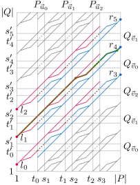
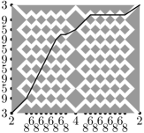
For , let be the index in of the central vertex of the -th copy of . Let be the index in of the last vertex at location in the second copy of of the -th copy of . Symmetrically, let be the index in of the first vertex at location in the fifth copy of in the -th copy of . Similarly, define and respectively to be the index in of respectively the first and last vertex of the -th copy of . We illustrate these indices in Figure 1.
For two curves of equal size, call a synchronous matching if . If and are orthogonal -dimensional boolean vectors, then the synchronous matching between and has width , so . Since is a Yes-instance, we can pick and such that and are orthogonal vectors. Let and . As depicted schematically in Figure 2, we construct a matching of width between and . This matching is composed of three matchings of width between the following pairs of curves: , and . These matchings are constructed in Lemmas 5.1 and 5.3.
Lemma 5.1.
Let and , then and .
Proof 5.2.
Observe that the synchronous matching has width for the following pairs of curves. Cases 1. and 2. as well as cases 3. and 4. are symmetric.
-
(1)
and ;
-
(2)
and ;
-
(3)
and with .
-
(4)
and with .
These matchings can be concatenated to obtain a matching of width between and , and between and .
Lemma 5.3.
If and are orthogonal, then a matching of width between and exists for with .
Proof 5.4.
We have . Since , we have . Since and are orthogonal, the synchronous matching between and has width . It remains to show that there exists a matching of width between (a) and , and between (b) and . We show case (a), the other case is symmetric. We have and . The synchronous matching between and has width , so it suffices to construct a matching between and . We illustrate such a matching in Figure 3. Recall that , so assume that . We can view as and as . The second and fourth parenthesized terms and in this view of can be matched to the second and fourth terms of this view of with width . Moreover, we can match the first, third, and fifth pairs of parenthesized terms in these views synchronously with width . Thus we obtain a matching of width between and .
Lemma 5.5.
If is a nontrivial Yes-instance of Orthog, then there is a matching of width between and for some .
Corollary 5.6.
If is a nontrivial Yes-instance of Orthog, then .
5.2. No-instance
Consider a No-instance of . To show that we construct of cut of width between and that starts on and ends on . Our cut consists of the following types of elementary pieces.
-
(1)
If all points of are at distance at least from , then there are cuts of width from to and from to .
-
(2)
Symmetrically, if all points of are at distance at least from , then there are cuts of width from to and from to .
-
(3)
If , there is a cut of width from to if and and either and or and .
-
(4)
Symmetrically if , there is a cut of width from to if and and either and or and .
Types 1. and 2. trivially provide cuts consisting of a single straight path. The cuts of types 3. and 4. are constructed in Lemma 5.7. Lemma 5.9 uses these to cut between and .
Lemma 5.7.
If , there is a cut of width from to if and and either and or and .
Proof 5.8.
Let and and suppose that and (the other case where and is symmetric). Let be the minimum value in for which , or if there is no such value. Then there is a straight cut of width from to . We show that is at distance at least from any point with . Indeed, . Hence, the straight cut from to also has width at least , so the composition of the straight cuts yields a cut of width from to .
Lemma 5.9.
If and are not orthogonal, then there is a cut of width between and that starts at and ends at .
Proof 5.10.
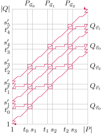
Since and are not orthogonal, for some index . Compose a cut of width (see also Figure 4) out of these elementary pieces: 3. from to ; 2. to ; copies of 4. to ; 1. to ; copies of 4. to ; 2. to ; and 3. to .
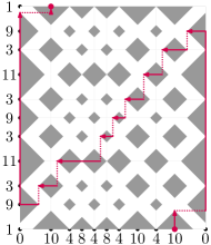
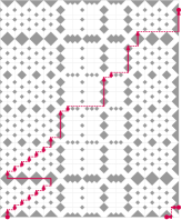

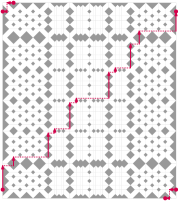
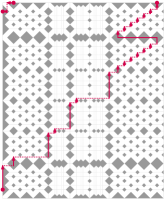


For the purpose of disambiguation, we will refer to the subcurve of simply as . The cuts given by Lemma 5.9 are connected as follows, as illustrated in Figures 2 and 5.
-
a.
For and , we cut from the end of the cut between and to the start of the cut between and .
-
b.
Furthermore, we cut from to the start of the cut between and .
-
c.
Similarly, we cut from the end of the cut between and to .
-
d.
Finally, for , we cut from to .
Composing these cuts yields a cut of width from to .
We believe that the illustrations of Figure 5 are more helpful than the formal definitions of such cuts. The cuts of types a., b., and c. start or end with the cut illustrated in the top and bottom of the second column of the top row of Figure 5. The remainder of the cuts of type a. is illustrated as the central cut in the third column of the top row. The cuts of type b. start as illustrated in the first column of the top row. Similarly, the cuts of type c. end as illustrated in the last column of the top row. The cuts of type d. are more complicated and start with the last column of the bottom row. Ignoring small cuts in corners, this cut is followed by the central cut of the second column of the top row, and the cut in the third column of the bottom row, repeated times, followed by a final copy of the central cut of the second column of the top row and the cut of the first column of the bottom row.
Whereas it should be evident why the cuts in the top row exist, this may not be clear for the cuts in the bottom row. In particular, a central elementary piece of type 1. exists only if the corresponding vector contains a one. However, this is the case since all vectors are nonzero, since our instance is nontrivial.
Lemma 5.11.
If is a nontrivial No-instance of Orthog, then there is a cut of width from to .
Corollary 5.12.
If is a nontrivial No-instance of Orthog, then .
Theorem 5.13.
For any polynomial restriction of , the partial Fréchet distance from to has no time -approximation unless SETH’ fails.
6. Fréchet distance
We use and to construct two curves and of size as follows.
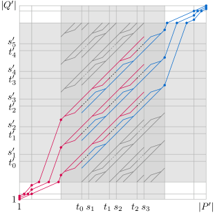
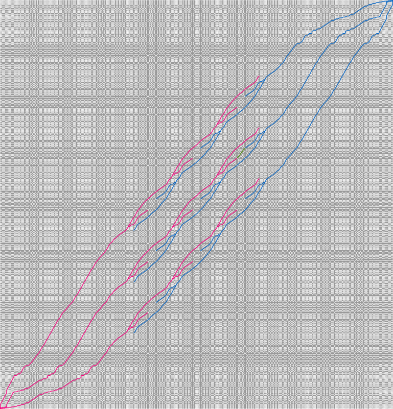
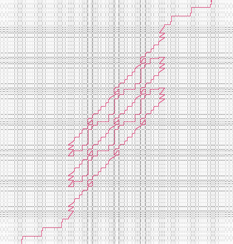
We show that if the nontrivial instance is a Yes-instance, and that otherwise (see also Figures 8 and 9). Hence, a time -approximation algorithm (with ) for the Fréchet distance violates SETH’.
Consider a nontrivial Yes-instance. Let and be the indices in of respectively the -th and -th vertices of the copy of in . For each , we construct a matching of width between and , and between and , see Figure 6. It then follows from Corollary 5.5 that .
We construct the matching between and , the other case is symmetric. Match with the first copies of . Match copies of with the remaining copies of . Match the remaining copies of with copies of . Match copies of with copies of . Match the next copy of with the remainder of . Finally, match the remainder of with .
Corollary 6.1.
If is a nontrivial Yes-instance of Orthog, then .
Now consider a nontrivial No-instance. Let be the index in of the last vertex at position of the first occurrence of . We construct a cut of width from a point on to the start of the copy of the cut given by Corollary 5.11. Similarly, we can construct a cut of width from the end of that cut to . We show how to construct the first cut, the other cut is symmetric.
Let be the index in of the last vertex (at position ) of of the last occurrence of . Consider the last two vertices of , namely those at positions and , respectively. Any point on has distance at least to the vertex at position . Similarly, for all vertices except the interior vertices of have distance at least to the vertex at position . The interior vertices of have distance at least to the vertex of at position . Let be index in of the last vertex of at position in the last occurrence of . We obtain a cut of width from to . Let and let be the index in of the second vertex (at location ) of . There is a type 3. cut of width from to . Finally, we construct a cut of width between and . The cut starts at and uses a cut of type 1. followed by cuts of type 3. and one cut of type 2. to reach the start of the cut given by Corollary 5.11.
Corollary 6.2.
If is a nontrivial No-instance of Orthog, then .
Theorem 6.3.
The Fréchet distance between one-dimensional curves and has no time -approximation unless SETH’ fails.
7. Discrete Fréchet distance
The previous constructions can easily be adapted to show that the discrete Fréchet distance cannot be approximated better than a factor in strongly subquadratic time. We adapt the constructed curves by introducing a constant number of vertices along each edge.
Higher-dimensional curves and generally have critical values. The Fréchet distance between and is always one of the critical values [4]. In contrast to curves in higher dimensions, where a critical value can depend on three vertices, critical values for curves in one dimension depend only on two vertices. In particular, for curves in one dimension, a critical value is either half the distance between two vertices of the same curve, or the distance between two vertices of different curves. If there are only distinct coordinates, this means there are critical values. Lemma 7.1 transforms curves into curves that are times as large, such that their discrete Fréchet distance is the Fréchet distance of the original curves. The curves in our construction have only a constant number of distinct coordinates, leading to Corollaries 7.4 and 7.5.
Lemma 7.1.
For continuous one-dimensional curves and with distinct coordinates, there are curves and of sizes and with .
Proof 7.2.
Let be the set of coordinates that lie at distance from a vertex of or . Let and be copies of and for which each edge is subdivided by introducing vertices at the points of on that edge. The curves and have and vertices respectively. Consider a matching between and of width . Then the discrete Fréchet distance between and is at most . Let be the union of for all critical values . Then . Consider the curves and of size and respectively. Then the discrete Fréchet distance between and is at most the Fréchet distance between and . Since the Fréchet distance is a lower bound for the discrete Fréchet distance, we have .
Remark 7.3.
In our construction, we can say something more: because the vertices of all have odd coordinates and the vertices of all have even coordinates, the critical values are all integer. Moreover, since all vertices lie in the range , the critical values of and are integers between and .
Corollary 7.4.
The discrete Fréchet distance between one-dimensional curves and has no time -approximation unless SETH’ fails.
Corollary 7.5.
For any polynomial restriction of , the partial discrete Fréchet distance from to has no time -approximation unless SETH’ fails.
8. Weak Fréchet distance
In this section we consider the weak Fréchet distance. The width of a path is . A (continuous) weak Fréchet matching between and is a path that starts at and ends at . The (continuous) weak Fréchet distance between and is the minimum width over all such matchings. In related work [11], a variant of the weak Fréchet distance which we will refer to as the weak Fréchet distance without endpoint restrictions was considered. This distance is defined analogously, except that we require and , and not that the path starts at and ends at .
We define the discrete weak Fréchet distance analogously, but for discrete matchings. Consider the graph with vertices and edges between pairs of vertices at distance , such that vertex has (undirected) edges to , , , and . A discrete weak Fréchet matching without endpoint restrictions between and consists of the set of vertices of a path in this graph, with the requirement that and . For a discrete weak Fréchet matching, this path starts at and ends at .
8.1. Discrete or higher-dimensional weak Fréchet distance
Our lower bound constructions for the weak Fréchet distance are similar to the one by Bringmann [7]. For a nontrivial instance of , we construct the following discrete curves and in one dimension:
Alternatively, we construct the following continuous curves and in two dimensions:
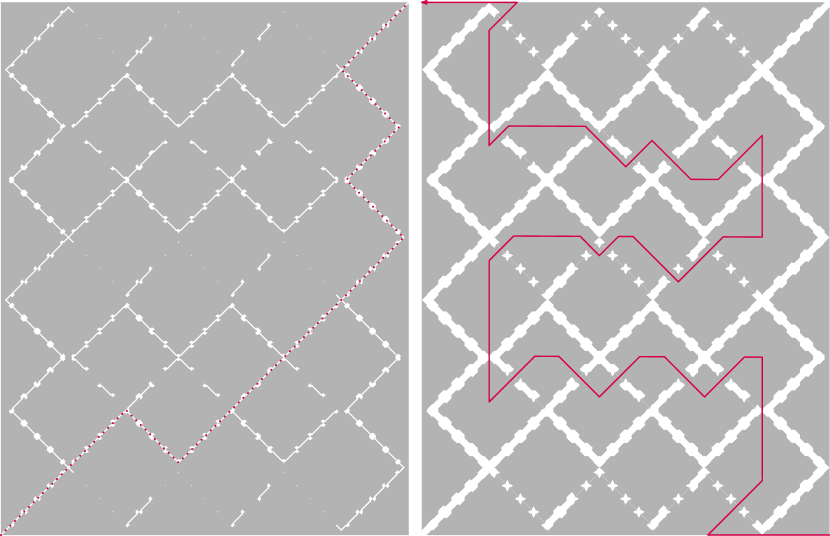
In both cases, the curves and have distance if and are orthogonal and distance otherwise. For a Yes-instance with orthogonal vectors and , match the first copy of with the first gadgets of type . Similarly, match the last copy of to the last gadgets of type . Match the copy of preceding with up until the gadget , match with and match the copy of after starting after the gadget of . This yields a matching of width . See Figure 7 (Left).
Conversely, a matching of width less than must traverse one of the curves and simultaneously, which is not possible for a No-instance. In the construction, any matching of width less than can be extended into one containing and . Hence, the reductions also apply to the weak Fréchet distance without endpoint restrictions.
Theorem 8.1.
For any polynomial restriction of , the discrete weak Fréchet distance between one-dimensional curves and (with and without endpoint restrictions) and the weak Fréchet distance (with and without endpoint restrictions) between two dimensional curves and , has no time -approximation unless SETH’ fails.
8.2. Continuous one-dimensional weak Fréchet distance
In this section, we show that the continuous weak Fréchet distance can be computed in linear time for curves in one dimension. For this case, the weak Fréchet distance without endpoint restrictions was already known to be computable in linear time, namely because it is equivalent to the Hausdorff distance between the images of those curves [11].
Our algorithm for computing the continuous weak Fréchet distance is more complicated. It will be helpful to transform the input curves into canonical ones. Let a canonical curve be a continuous one-dimensional curve that contains no four consecutive vertices with or . By repeating the transformation of Lemma 8.2, one can in linear time transform any continuous one-dimensional curve into a canonical curve with .
Lemma 8.2.
Let be a continuous one-dimensional curve that is not canonical due to vertices . Let be the copy of with the edges between and replaced by a single edge, then .
Proof 8.3.
Assume that (otherwise we are done). Then for and for . Pick and such that and and . Then the piecewise linear path with vertex sequence , , , , , and is a weak Fréchet matching of width .
Canonical curves have the following structural properties.
Lemma 8.4.
For a canonical curve and any , any shortest edge of has or as an endpoint.
Proof 8.5.
Otherwise the shortest edge of is surrounded by edges that are at least as long and hence form a witness that is not canonical.
Corollary 8.6.
For any canonical curve, the subsequence of local maxima is quasiconcave, the subsequence of local minima is quasiconvex, and the vertices that are global minima or maxima (of which there are at most three) are all consecutive.
A growing curve is any canonical curve whose last edge contains both a global maximum and minimum. For a point and a curve , let be the distance from to the closest point on . Our algorithm for the weak Fréchet distance uses the following linear-time subroutine.
Algorithm 8.7.
| GreedyMatching: | |||||
| = | |||||
| = | |||||
| = | |||||
| while or : | |||||
| if and : | |||||
| = | |||||
| else if : | |||||
| = | |||||
| = | |||||
| else if : | |||||
| = | |||||
| = | |||||
| return |
Lemma 8.8.
Algorithm 8.7 computes for growing curves and , the minimum width over all paths from to any .
Proof 8.9.
Let . We use as invariant that (1) there is a path of width from to some , and that (2) there are no paths of width less than to any . Indeed, this invariant holds at the start of the loop. When the algorithm returns we have and as desired, so it remains to show that the invariant is maintained. Part (1) of the invariant is maintained by construction, so it suffices to show that part (2) is maintained.
Fix some and suppose that the invariant is satisfied. It will clearly be maintained for the next iteration if or , as any path to or must also enter . So assume that and . Suppose for a contradiction that the invariant does not hold for the values of after the next iteration, then there is a path of width with from to a point outside . Let be the point where leaves . Then either or . If , then . Similarly, if , then . As both cases give a contradiction, the invariant is maintained.
Lemma 8.10.
The weak Fréchet distance for canonical curves is computable in linear time.
Proof 8.11.
Consider canonical curves and . If one curve has a single vertex, the weak Fréchet distance is its distance to the furthest point on the other curve. Consider an edge between a global minimum and maximum of . Define the growing curves , and . Similarly, consider such an edge of and define and analogously. Let and .
We show that . For this, consider a weak Fréchet matching of width between and . Define as the map for which is the unique point with for , and for . Define a path by replacing any point by . Then is a path of width at most from to a point . Thus and by symmetric argument .
It remains to show that . There exists a path of width from to . There also is a path of width from to . Connecting these paths with the straight segment from to yields a weak Fréchet matching of the desired width.
Theorem 8.12.
The weak Fréchet distance between continuous one-dimensional curves can be computed in linear time.
Proof 8.13.
Transform input curves and into canonical curves and in linear time. By triangle inequality we have , which can be computed in linear time by Lemma 8.10.
9. Discussion
We have shown that the Fréchet and many of its variants cannot be approximated better than factor in strongly subquadratic time unless SETH’ fails. Although we show that similar reductions cannot improve upon this factor, it remains open whether this factor is tight, or if there is a strongly subquadratic constant factor approximation at all. Furthermore, for curves in D, our construction for the Fréchet distance does not rule out a strongly subquadratic algorithm for curves with an imbalanced number of vertices.
References
- [1] Amir Abboud, Karl Bringmann, Holger Dell, and Jesper Nederlof. More consequences of falsifying SETH and the orthogonal vectors conjecture. In Proc. 50th Sympos. Theory Comput. (STOC), pages 253–266, 2018.
- [2] Pankaj K Agarwal, Rinat Ben Avraham, Haim Kaplan, and Micha Sharir. Computing the discrete Fréchet distance in subquadratic time. SIAM J. Comput., 43(2):429–449, 2014.
- [3] Helmut Alt and Maike Buchin. Can we compute the similarity between surfaces? Discrete Comput. Geom. (DCG), 43(1):78–99, 2010.
- [4] Helmut Alt and Michael Godau. Computing the Fréchet distance between two polygonal curves. Internat. J. Comput. Geom. Appl. (IJCGA), 5(1–2):75–91, 1995.
- [5] Boris Aronov, Sariel Har-Peled, Christian Knauer, Yusu Wang, and Carola Wenk. Fréchet distances for curves, revisited. In Proc. 14th European Sympos. Algorithms (ESA), pages 52–63, 2006.
- [6] Sotiris Brakatsoulas, Dieter Pfoser, Randall Salas, and Carola Wenk. On map-matching vehicle tracking data. In Proc. 31st International Conference on Very Large Data Bases, pages 853–864. VLDB Endowment, 2005.
- [7] Karl Bringmann. Why walking the dog takes time: Fréchet distance has no strongly subquadratic algorithms unless SETH fails. In Proc. 55th Sympos. Found. Comput. Sci. (FOCS), pages 661–670, 2014.
- [8] Karl Bringmann and Marvin Künnemann. Improved approximation for Fréchet distance on -packed curves matching conditional lower bounds. Internat. J. Comput. Geom. Appl. (IJCGA), 27(1-2):85–120, 2017.
- [9] Karl Bringmann and Wolfgang Mulzer. Approximability of the discrete Fréchet distance. J. Computational Geometry (JoCG), 7(2):46–76, 2016.
- [10] Kevin Buchin, Maike Buchin, David Duran, Brittany Terese Fasy, Roel Jacobs, Vera Sacristán, Rodrigo I. Silveira, Frank Staals, and Carola Wenk. Clustering trajectories for map construction. In Proc. 25thInternat. Conf. on Advances in Geographic Information Systems (SIGSPATIAL), pages 14:1–14:10, 2017.
- [11] Kevin Buchin, Maike Buchin, Christian Knauer, Günter Rote, and Carola Wenk. How difficult is it to walk the dog. In Proc. 23rd European Workshop on Computational Geometry (EuroCG), pages 170–173, 2007.
- [12] Kevin Buchin, Maike Buchin, Wouter Meulemans, and Wolfgang Mulzer. Four soviets walk the dog: Improved bounds for computing the Fréchet distance. Discrete Comput. Geom. (DCG), 58(1):180–216, 2017.
- [13] Kevin Buchin, Maike Buchin, and André Schulz. Fréchet distance of surfaces: Some simple hard cases. In Proc. 18th European Sympos. Algorithms (ESA), pages 63–74, 2010.
- [14] Kevin Buchin, Maike Buchin, and Yusu Wang. Exact algorithms for partial curve matching via the Fréchet distance. In Proc. 20th Sympos. Discrete Algorithms (SODA), pages 645–654, 2009.
- [15] Kevin Buchin, Jinhee Chun, Maarten Löffler, Aleksandar Markovic, Wouter Meulemans, Yoshio Okamoto, and Taichi Shiitada. Folding free-space diagrams: Computing the Fréchet distance between 1-dimensional curves (multimedia contribution). In Proc. 33rd Sympos. Comput. Geom. (SoCG), pages 64:1–64:5, 2017.
- [16] Kevin Buchin, Tim Ophelders, and Bettina Speckmann. Computing the similarity between moving curves. In Proc. 23rd European Sympos. Algorithms (ESA), pages 928–940, 2015.
- [17] Atlas F. Cook and Carola Wenk. Geodesic Fréchet distance inside a simple polygon. Transactions on Algorithms, 7(1):Art. 9, 2010.
- [18] Anne Driemel and Sariel Har-Peled. Jaywalking your dog: Computing the fréchet distance with shortcuts. SIAM J. Comput., 42(5):1830–1866, 2013.
- [19] Anne Driemel, Sariel Har-Peled, and Carola Wenk. Approximating the Fréchet distance for realistic curves in near linear time. Discrete & Computational Geometry, 48(1):94–127, 2012.
- [20] Anne Driemel, Amer Krivosija, and Christian Sohler. Clustering time series under the Fréchet distance. In Proc. 27th Sympos. Discrete Algorithms (SODA), pages 766–785, 2016.
- [21] Thomas Eiter and Heikki Mannila. Computing discrete fréchet distance. Technical Report CD-TR 94/64, Information Systems Department, Technical University of Vienna, 1994.
- [22] Joachim Gudmundsson and Thomas Wolle. Towards automated football analysis: Algorithms and data structures. In Proc. 10th Australasian Conf. on Mathematics and Computers in Sport, 2010.
- [23] Sariel Har-Peled and Benjamin Raichel. The Fréchet distance revisited and extended. Transactions on Algorithms, 10(1):3, 2014.
- [24] Daniel Kane and Ryan Williams. The orthogonal vectors conjecture for branching programs and formulas. arXiv preprint arXiv:1709.05294, 2017.
- [25] Maximilian Konzack, Thomas McKetterick, Tim Ophelders, Maike Buchin, Luca Giuggioli, Jed Long, Trisalyn Nelson, Michel A Westenberg, and Kevin Buchin. Visual analytics of delays and interaction in movement data. Internat. J. of Geographical Information Science, 31(2):320–345, 2017.
- [26] Amir Nayyeri and Hanzhong Xu. On computing the Fréchet distance between surfaces. In Proc. 32nd Sympos. Comput. Geom. (SoCG), pages 55:1–55:15, 2016.
- [27] Ryan Williams. A new algorithm for optimal constraint satisfaction and its implications. In Proc. 31st Internat. Colloq. Automata Lang. Program. (ICALP), pages 1227–1237, 2004.
Appendix A Figures accompanying Section 6
