∎
22email: e.s.riis@damtp.cam.ac.uk 33institutetext: Matthias J. Ehrhardt 44institutetext: Department of Applied Mathematics and Theoretical Physics, University of Cambridge, UK
44email: m.j.ehrhardt@damtp.cam.ac.uk 55institutetext: G. R. W. Quispel 66institutetext: Department of Mathematics and Statistics, La Trobe University, Victoria 3086, Australia
66email: r.quispel@latrobe.edu.au 77institutetext: Carola-Bibiane Schönlieb 88institutetext: Department of Applied Mathematics and Theoretical Physics, University of Cambridge, UK
88email: cbs31@cam.ac.uk
A geometric integration approach to nonsmooth, nonconvex optimisation††thanks: All authors acknowledge support from CHiPS (Horizon 2020 RISE project grant). E. S. R, M. J. E. and C.-B. S. acknowledge support from the Cantab Capital Institute for the Mathematics of Information. M. J. E. and C.-B. S. acknowledge support from Leverhulme Trust project “Breaking the non-convexity barrier”, EPSRC grant “EP/M00483X/1”, and EPSRC centre “EP/N014588/1”. G. R. W. Q. acknowledges support from the Australian Research Council, and is grateful to the Mittag-Leffler Institute for a productive stay. Moreover, C.-B. S. acknowledges support from the RISE project NoMADS and the Alan Turing Institute.
Abstract
The optimisation of nonsmooth, nonconvex functions without access to gradients is a particularly challenging problem that is frequently encountered, for example in model parameter optimisation problems. Bilevel optimisation of parameters is a standard setting in areas such as variational regularisation problems and supervised machine learning. We present efficient and robust derivative-free methods called randomised Itoh–Abe methods. These are generalisations of the Itoh–Abe discrete gradient method, a well-known scheme from geometric integration, which has previously only been considered in the smooth setting. We demonstrate that the method and its favourable energy dissipation properties are well-defined in the nonsmooth setting. Furthermore, we prove that whenever the objective function is locally Lipschitz continuous, the iterates almost surely converge to a connected set of Clarke stationary points. We present an implementation of the methods, and apply it to various test problems. The numerical results indicate that the randomised Itoh–Abe methods are superior to state-of-the-art derivative-free optimisation methods in solving nonsmooth problems while remaining competitive in terms of efficiency.
Keywords:
Geometric numerical integration discrete gradient methods derivative-free optimisation nonconvex optimisation nonsmooth optimisation Clarke subdifferential bilevel optimisationMSC:
49M25 49Q15 65K10 90C15 90C26 90C56 94A081 Introduction
We consider the unconstrained optimisation problem
| (1.1) |
where the objective function is locally Lipschitz continuous, bounded below and coercive—the latter meaning that is compact for all . The function may be nonconvex and nonsmooth, and we assume no knowledge besides point evaluations . To solve (1.1), we present randomised Itoh–Abe methods, a generalisation of the Itoh–Abe discrete gradient method. The latter is a derivative-free optimisation scheme,111Not to be confused with another derivative-free method with the same name proposed by Bagirov et al. (bag08, ), which uses a different concept of a discrete gradient. that has previously only been considered for differentiable functions.
Discrete gradient methods, a tool from geometric numerical integration, are optimisation schemes that inherit the energy dissipation of continuous gradient flow. The iterates of the methods monotonically decrease the objective function, for all time steps, and Grimm et al. (gri17, ) recently provided a convergence theory for solving (1.1) in the continuously differentiable setting. We extend the concepts and results of their work and show that the Itoh–Abe discrete gradient method can be applied in the nonsmooth case, and, furthermore, that the favourable dissipativity property of the methods extends to this setting. Furthermore, we prove that for locally Lipschitz continuous functions the iterates converge to a set of stationary points, defined by the Clarke subdifferential framework.
1.1 Gradient flow and the discrete gradient method
For a differentiable function , gradient flow is the ODE system defined by
| (1.2) |
where the dot represents differentiation with respect to time. By applying the chain rule, we compute
| (1.3) |
where denotes the 2-norm . This implies that gradient flow is inherently an energy dissipative system.
In the field of geometric numerical integration, one studies methods for numerically solving ODEs that also preserve structures of the continuous system—see (hai06, ; mcl01, ) for an introduction. Discrete gradient methods can be applied to first-order gradient systems to preserve energy conservation laws, dissipation laws, as well as Lyapunov functions (gon96, ; ito88, ; mcl99, ; qui96, ). They are defined as follows.
Definition 1.1
Let be continuously differentiable. A discrete gradient is a continuous mapping that satisfies the two following properties.
We now introduce the discrete gradient method for optimisation. For and time steps , , we solve
| (1.4) |
We apply the above mean value property to derive that the iterates decrease .
| (1.5) |
Note that the decrease holds for all time steps , and that (1.5) can be seen as a discrete analogue of the dissipative structure of gradient flow (1.3), replacing derivatives by finite differences.
Grimm et al. (gri17, ) proved that for coercive, continuously differentiable functions, the iterates of (1.4) converge to a set of stationary points, provided that there are strictly positive constants such that for all .
1.1.1 Itoh–Abe methods
The Itoh–Abe discrete gradient (ito88, ) (also known as coordinate increment discrete gradient)222There are infinitely many discrete gradients, each with a corresponding discrete gradient method. See (gri17, ) for further examples. is defined as
Solving an iterate of the discrete gradient method (1.4) with the Itoh–Abe discrete gradient is equivalent to successively solving scalar equations of the form
We generalise the Itoh–Abe discrete gradient method to randomised Itoh–Abe methods accordingly. Let be a sequence of directions, where denotes the unit sphere . The directions can be drawn from a random distribution or chosen deterministically. At the th step, we update
| (1.6) |
If no such exists, we set . We formalise this method in Algorithm 1. We assume throughout the paper that the time steps are bounded between two strictly positive constants , which can take arbitrary values.
Input: starting point , directions , time steps .
Observe that if cycle through the standard coordinates with the rule , then computing steps of (1.6) corresponds to one step of (1.4) with the Itoh–Abe discrete gradient. Furthermore, the dissipation properties (1.5) can be rewritten as
| (1.7) |
Consequently, the dissipative structure of the Itoh–Abe methods is well-defined in a derivative-free setting.
Ehrhardt et al. (rii18smooth, ) studied Itoh–Abe methods in the smooth setting, asserting linear convergence rates for functions that satisfy the Polyak–Łojasiewicz inequality (kar16, ). Furthermore, the application of Itoh–Abe discrete gradient methods to smooth optimisation problems is well-documented. Applications include convex variational regularisation problems for image analysis (gri17, ), nonconvex image inpainting problems with Euler’s elastica regularisation (rin17, ), for which it outperformed gradient-based schemes, and the popular Gauss–Seidel method and successive-over-relaxation (SOR) methods for solving linear systems (miy17, ).
1.2 Bilevel optimisation and blackbox problems
An important application for developing derivative-free solvers is model parameter optimisation problems. The setting for this class of problems is as follows. A model depends on some tunable parameters , so that for a given parameter choice , the model returns an output . There is a cost function , which assigns to output a numerical score , which we want to minimise. The associated model parameter optimisation problem becomes
A well-known example of parameter optimisation problems is supervised machine learning.
In this paper, we consider one instance of such problems in image analysis, called bilevel optimisation of variational regularisation problems. Here, the model is given by a variational regularisation problem for image denoising,
where is a noisy image and is the regularisation parameter. For training data with desired reconstruction , we consider a scoring function that estimates the discrepancy between and the reconstruction . In Section 6.2, we apply Itoh-Abe methods to solve these problems.
Bilevel optimisation problems, and model parameter optimisation problems in general, pose several challenges. They are often nonconvex and nonsmooth, due to the nonsmoothness and nonlinearity of . Furthermore, the model simulation is an algorithmic process for which gradients or subgradients cannot easily be estimated. Such problems are termed blackbox optimisation problems, as one only has access to point evaluations of the function. It is therefore of great interest to develop efficient and robust derivative-free methods for such optimisation problems.
There is a rich literature on bilevel optimisation for variational regularisation problems in image analysis, c.f. e.g. (cal15, ; de17, ; kun13, ; och15, ). Furthermore, model parameter optimisation problems appear in many other applications. These include optimising for the management of water resources (fow08, ), approximation of a transmembrane protein structure in computational biology (gra04, ), image registration in medical imaging (oeu07, ), the building of wind farms (dup16, ), and solar energy utilisation in architectural design (kam10, ), to name a few.
1.3 Related literature on nonsmooth, nonconvex optimisation
Although nonsmooth, nonconvex problems are known for their difficulty compared to convex problems, a rich optimisation theory has grown since the 1970s. As the focus of this paper is derivative-free optimisation, we will compare the methods’ convergence properties and performance to other derivative-free solvers. Audet and Hare (aud17, ) recently provided a reference work for this field.
While there a myriad of derivative-free solvers, few provide convergence guarantees for nonsmooth, nonconvex functions. Audet and Dennis Jr (aud06, ) introduced the mesh adaptive direct search (MADS) method for constrained optimisation, with provable convergence guarantees to stationary points for nonsmooth, nonconvex functions. Direct search methods evaluate the function at a finite polling set, compare the evaluations, and update the polling set accordingly. Such methods only consider the ordering of the evaluations, rather than the numerical differences. A significant portion of derivative-free methods are direct search methods, and the most well known of these is the Nelder–Mead method (also known as the downhill simplex method) (nel65, ).
Alternatively, model-based methods that build a local quadratic model based on evaluations are well-documented (car18, ; pow06, ; pow09, ). While such methods tend to work well in practice, they are normally designed only for smooth functions, so their performance on nonsmooth functions is not guaranteed.
Fasano et al. (fas14, ) formulated a derivative-free line search method termed DFN and analyse its convergence properties for nonsmooth functions for the Clarke subdifferential, in the constrained setting. The Itoh–Abe methods share many similarities with DFN, such as performing line searches along dense directions, and they employ a similar convergence analysis. However, the line searches of these methods differ, and the Itoh–Abe methods are in particular motivated by discrete gradient methods and preserving the dissipative structure of gradient flow. Furthermore, our convergence analysis is more comprehensive, considering both stochastic and deterministic methods, as well as obtaining stronger convergence results in the deterministic case. Building on the aforementioned algorithm, Liuzzi and Truemper (liu17, ) formulated a derivative-free method that is a hybrid between DFN and MADS.
Furthermore, we note the resemblance of randomised Itoh–Abe methods (1.6), when is randomly, independently drawn from , to the random search method proposed by Polyak in (pol87, ) and studied for nonsmooth, convex functions by Nesterov in (nes17, ), given by
where is randomly, independently drawn from . The implicit equation (1.6) can be treated as a line search rule for the above method, with constraints imposed by , .
While our focus is on derivative-free methods, we also mention some popular methods for nonsmooth, nonconvex optimisation that use gradient or subgradient information. Central in nonsmooth optimisation are bundle methods, where a subgradient (cla90, ) is required at each iterate to construct a linear approximation to the objective function—see (kiw85, ) for an introduction. A close alternative to bundle methods are gradient sampling methods (see (bur18, ) for a recent review by Burke et al.), where the descent direction is determined by sampling gradients in a neighborhood of the current iterate. Curtis and Que (cur15, ) formulated a hybrid method between the gradient sampling scheme of (cur13, ) and the well known quasi-Newton method BFGS adapted to nonsmooth problems (lew13, ). These methods have convergence guarantees in the Clarke subdifferential framework, under the assumption that the objective function is differentiable on an open, dense set. Last, we mention a derivative-free scheme based on gradient sampling methods, proposed by Kiwiel (kiw10, ), where gradients are replaced by Gupal’s estimates of gradients of the Steklov averages of the objective function. This method has convergence guarantees in the Clarke subdifferential framework, but has a high computational cost in terms of function evaluations per iterate.
1.4 Contributions
In this paper, we formulate randomised Itoh–Abe methods for nonsmooth functions. We prove that the method always admits a solution, and that the iterates converge to a set of Clarke stationary points, for any locally Lipschitz continuous function, and both for deterministic and randomly chosen search directions. Consequently, the scope of discrete gradient methods for optimisation is significantly broadened, and we conclude that the dissipativity properties of gradient flow can be preserved even beyond differentiability. Ultimately, this provides a new, robust, and versatile optimisation scheme for nonsmooth, nonconvex functions.
The theoretical convergence analysis for the Itoh–Abe methods is thorough and foundational, and we provide examples that demonstrate that the conditions of the convergence theorem are not just sufficient, but necessary. Furthermore, the statements and proofs are sufficiently general so that they can be adapted to other schemes, such as the aforementioned DFO method, thus enhancing the theory of these methods as well.
We show that the method works well in practice, by solving bilevel optimisation problems for variational regularisation problems, as well as solving benchmark problems such as Rosenbrock functions.
The rest of the paper is structured as follows. Section 2 provides a background on the Clarke subdifferential for nonsmooth, nonconvex analysis. In Section 3, the main theoretical results of the paper are presented, namely existence and optimality results in the stochastic and deterministic setting. In Section 4, we briefly discuss the Itoh–Abe discrete gradient for general coordinate systems. In Section 5 and Section 6, the numerical implementation is described and results from example problems are presented. Finally, a conclusion is given in Section 7.
2 Nonconvex optimisation
In this section, we introduce the Clarke subdifferential framework (cla90, ) for nonsmooth, nonconvex optimisation. This is the most popular framework for this setting, due to its nice analytical properties. It generalises the gradient of a differentiable function, as well as the subdifferential (eke99, ) of a convex function, hence the term Clarke subdifferential. Francis H. Clarke introduced the framework in his doctoral thesis in 1973 (cla73, ), in which he termed it generalised gradient.
2.1 The Clarke subdifferential
Throughout the paper, for and , we denote by the open ball .
Definition 2.1
is Lipschitz of rank near if there exists such that for all , one has
is locally Lipschitz continuous if the above property holds for all .
Definition 2.2
For Lipschitz near and for a vector , the Clarke directional derivative is given by
Definition 2.3
Let be locally Lipschitz and . The Clarke subdifferential of at is given by
An element of is called a Clarke subgradient.
The subdifferential is well-defined for locally Lipschitz functions, coincides with the standard subdifferential for convex functions (cla90, , Proposition 2.2.7), and coincides with the derivative at points of strict differentiability (cla90, , Proposition 2.2.4). It can equivalently be characterised as
where is the set of differentiable points, and denotes the convex hull of the set (cla90, , Theorem 2.5.1). We additionally state two useful results, both of which can be found in Chapter 2 of (cla90, ).
Proposition 2.4
Suppose is locally Lipschitz continuous. Then
-
(i)
is nonempty, convex and compact, and if is Lipschitz of rank near , then .
-
(ii)
is outer semicontinuous. That is, for all , there exists such that
There are alternative frameworks for generalising differentiability of nonsmooth, nonconvex functions. For example, the Michel–Penot subdifferential (mic84, ) coincides with the Gâteaux derivative when this exists, unlike the Clarke subdifferential, which is larger and only coincides with strict derivatives (gil99, ). However, the Clarke subdifferential is outer semicontinuous, making it in most cases the preferred framework for analysis. See (bor99, ) by Borwein and Zhu for a survey of various subdifferentials, published on the 25th birthday of the Clarke subdifferential.
2.1.1 Discrete gradients versus subgradients
By definition, when is continuously differentiable, any discrete gradient converges to the gradient as . However, for nondifferentiable , discrete gradients do not necessarily approximate a subgradient or even an -approximate subgradient.333For convex functions, is an -approximate subgradient if, for all , we have (hin01, ). This is demonstrated by the following example.
Example 2.5
Let , and set and . Then, for all , the Itoh–Abe discrete gradient is
Thus, , and . However, is not in . In fact, for all , we have .
2.1.2 Clarke stationary points
Definition 2.6
is a Clarke stationary point of if .
For our purposes, we also define Clarke directional stationarity.
Definition 2.7 (Directional Clarke stationarity)
For a direction , we say that is Clarke directionally stationary at along if
Remark 2.8
A point is Clarke stationary if and only if is Clarke directionally stationary at along for all such that .
Any local maxima and minima are stationary. If is convex, then stationary points coincide with the global minima. For more general classes of functions, the concept of Clarke stationary points also reduces to convex first-order optimality conditions.
Definition 2.9 ((pen97, ))
A locally Lipschitz continuous function is pseudoconvex if, for all ,
If is pseudoconvex, then any Clarke stationary point is a global minimum (aus98, ). Clarke (cla90, ) also introduced the notion of regularity.
Definition 2.10
A function is regular at if the directional derivative
exists for all and . If this holds for all , we say that is regular.
For a regular function, a point is Clarke stationary if and only if the directional derivative is nonnegative in all directions. For example, convex functions are regular, and strict differentiability at a point implies regularity at a point. However, for nonregular functions, can simultaneously be Clarke stationary and have negative directional derivatives in a neighbourhood of directions.
3 The discrete gradient method for nonsmooth optimisation
In this section, we present the main theoretical results for the randomised Itoh–Abe methods. In particular, we prove that the update (1.6),
admits a solution for all . We also prove under minimal assumptions on and that the iterates converge to a connected set of Clarke stationary points, both in a stochastic and deterministic setting.
3.1 Existence result
Lemma 3.1
Suppose is a continuous function bounded below, and that , and . Then one of the following statements hold.
-
(i)
There is a that solves (1.6), i.e. that satisfies .
-
(ii)
is Clarke directionally stationary at along .
Proof
Suppose the second statement does not hold. Then there is such that
so assume without loss of generality that . By definition of , there is such that for all ,
Taking , we get that
so there is a such that
On the other hand, as is bounded below, we have
Thus there is such that
Since the mapping is continuous for , we conclude by the intermediate value theorem (rud76, , Theorem 4.23) that there is that solves the discrete gradient equation
Remark 3.2
Note that by the above proof it is straightforward to identify an interval in which a solution to (1.6) exists, allowing for the use of standard root solver algorithms.
The following lemma, which is an adaptation of (gri17, , Theorem 1) for the nonsmooth setting, summarises some useful properties of the methods.
Lemma 3.3
Suppose that is continuous, bounded from below and coercive, and let be the iterates produced by (1.6). Then, the following properties hold.
-
(i)
.
-
(ii)
.
-
(iii)
.
-
(iv)
has an accumulation point .
Proof
Property (i) follows from the equation .
Next we show properties (ii) and (iii). Since is bounded below and is decreasing, for some limit . Therefore, by (1.7)
Similarly, by (1.7)
We conclude
which shows properties (ii) and (iii).
Last, we show (iv). Since is a decreasing sequence, the iterates belong to the set . Therefore, by coercivity of , the iterates are bounded, and admit an accumulation point.
We denote by the limit set of , which is the set of accumulation points,
By the above lemma, is nonempty. We now prove further properties of the limit set.
Lemma 3.4
The limit set is compact, connected and has empty interior. Furthermore, is constant on .
Proof
Boundedness of follows from coercivity of combined with the fact that belongs to the level set . Since any accumulation point of is also an accumulation point of , is closed. Hence is compact.
We prove connectedness by contradiction. Suppose there are two disjoint, nonempty open sets and such that . The sequence jumps between and infinitely many times and , which implies that there is a subsequence of in . However, is a bounded sequence and has an accumulation point, which must belong in . This contradicts the assumption that all accumulation points of are in .
We show that has empty interior by contradiction. Suppose contains an open ball in . Then as , there is a such that . However, as takes the same value on all of , we deduce that . Since is a decreasing sequence, for all . It follows from (1.7) that for all . Therefore, , which contradicts the assumption that has nonempty interior.
Last, since is a decreasing sequence and for all , it follows that is constant on .
3.2 Optimality result
We now proceed to the main result of this paper, namely that all points in the limit set are Clarke stationary. We consider the stochastic case and the deterministic case separately.
In the stochastic case, we assume that the directions are randomly, independently drawn, and that the support of the probability density of is dense in . It is straightforward to extend the proof to the case where are drawn as an orthonormal system under the assumptions that the directions are independently drawn from and that the support of the density of the corresponding marginal distribution is dense in .
We define to be the set of nonstationary points,
| (3.1) |
Theorem 3.5
Let solve (1.6) where are independently drawn from the random distribution , and suppose that the support of the density of is dense in . Then , i.e. the limit set is almost surely in the set of stationary points.
Proof
We will construct a countable collection of open sets , such that and so that for all we have . Then the result follows from countable additivity of probability measures.
First, we show that for every , there is , , and such that
| (3.2) |
To show this, note that if , then by definition there is and such that
Therefore, there is such that for all and all , we have
As is Lipschitz continuous around , it is clear that the mapping
is also locally Lipschitz continuous (of the same rank). It follows that there exists such that for all , all , and all , we have
This concludes the first part.
Next, for , we define the set
Clearly
Let be a dense sequence in , which exists because is both countable and dense in . We define , where . Therefore,
Since a countable union of countable sets is countable, we conclude with the following statement. For each there is , , and , such that for all , all , and all , we have
and such that
| (3.3) |
Finally, we show that for each , almost surely, . For a given , write , and define , . We argue accordingly: The existence of an accumulation point of in would imply that there is a subsequence . Suppose and , so that for some . If , then
However,
so, combining these equations, we get
This in return implies
On the other hand, if , then
Setting , it follows that whenever and , then
Choosing such that , we know that this event only has to occur times for to leave . In other words, almost surely, there is no subsequence . This concludes the proof.
3.2.1 Deterministic case
We now cover the deterministic case, in which is required to be cyclically dense.
Definition 3.6
A sequence is cyclically dense in if, for all , there is such that for any , the set forms an -cover of ,
Remark 3.7
Randomly drawn sequences are almost surely not cyclically dense, hence the separate treatment of the stochastic and deterministic methods.
Many constructions of dense sequences are also cyclically dense. We provide an example of such a sequence on the unit interval .
Example 3.8
Let be an irrational number and define the sequence in by
where denotes the largest integer less than or equal to .
To see that is cyclically dense in , set and note by sequential compactness of that there is such that . We can write , where we know that is strictly positive, as no value can be repeated in the sequence due to being irrational. By modular arithmetic, we have for any ,
In other words, the subsequence moves in increments of on . Setting , where denotes the smallest integer greater than or equal to , it is clear that for any , the set forms an -cover of .
One could naturally extend this construction to higher dimensions , by choosing irrational numbers such that the ratio of any two of these numbers is also irrational.
Theorem 3.9
Let solve (1.6), where are cyclically dense. Then all accumulation points satisfy .
Proof
We consider the setup in the proof to Theorem 3.5, where is the set of nonstationary points (3.1) and is covered by a countable collection of open balls (3.3),
We will show that an accumulation point cannot belong to the ball , from which it follows that is a subset of the set of stationary points. For contradiction, suppose that there is a subsequence . By Lemma 3.3 (iii), since as , we deduce that for any , there is such that
By cyclical density, we can choose such that the corresponding directions form an -cover of . Therefore, there exists and , so we can argue as in Theorem 3.5, that
where . If had a limit in , this would happen arbitrarily many times, which is a contradiction. This concludes the proof.
3.3 Necessity of search density and Lipschitz continuity
For nonsmooth problems, it is necessary to employ a set of directions larger than the set of basis coordinates . To see this, consider the function and the starting point . With the standard Itoh–Abe discrete gradient method, the iterates would remain at , even though this point is nonstationary.
We show with a simple example that the assumption of density of in Theorem 3.5 is not only sufficient, but also necessary.
Example 3.10
We suppose is defined by for some , and set . For , let . Then is a direction of descent if and only if . This interval can be made arbitrarily small by choosing to be sufficiently large. Therefore, for an Itoh–Abe method to descend from for arbitrary functions, the directions need to include a convergent subsequence to the direction . As this direction is arbitrary, we deduce that must be dense.
Theorem 3.5 also assumes that is locally Lipschitz continuous. We briefly discuss why this assumption is necessary, and provide an example to show that for functions that are merely continuous, the theorem no longer holds.
By Proposition 2.1.1. (b) in (cla90, ), the mapping is upper semicontinuous for in a neighbourhood of , due to the local Lipschitz continuity of near . That is,
This property is crucial for the convergence analysis of Itoh–Abe methods, as it implies
Without local Lipschitz continuity, it is possible to have
In this case, there is no guarantee that the limit is Clarke stationary. We demonstrate this with an example.
Example 3.11
We will first state the iterates and then construct a function that fits these iterates. Let be a cyclically dense sequence in and assume without loss of generality that . Replacing with does not change the step in (1.6), so we assume that for all . We set and define and to be
Since , it follows that converges to some limit , and clearly decreases to a limit . Furthermore, these steps satisfy (1.6) with . We then define on the line segments by interpolating linearly from to .
Next, we define on as a function that linearly decreases everywhere in the direction , and so that its value is consistent with the values given on the predefined line segments . Note that this is a well-defined and continuous function, since each line in the direction crosses at most one point on at most one line segment, due to our assumptions on .
We conclude the example by noting that the limit is not Clarke stationary—in fact, no point is Clarke stationary—since for all .
3.4 Nonsmooth, nonconvex functions with further regularity
For a large class of nonsmooth optimisation problems (convex and nonconvex), the objective function is sufficiently regular so that the standard Itoh–Abe discrete gradient method is also guaranteed to converge to Clarke stationary points. These are functions for which is Clarke stationary if and only if for . One example is functions of the form
where is a continuously differentiable function that may be nonconvex, denotes , and . See for example Proposition 2.3.3 and the subsequent corollary in (cla90, ), combined with the fact that the nonsmooth component of , i.e. , separates into coordinate-wise scalar functions. This implies that the Clarke subdifferential is given by
where denotes the Cartesian product and
Since this paper is chiefly concerned with the blackbox setting where no particular structure of is assumed, we do not include a rigorous analysis of the convergence properties of the standard Itoh–Abe discrete gradient method for functions of the above form. However, we point out that for nonsmooth, nonconvex optimisation problems where Clarke stationarity is equivalent to Clarke directional stationarity along the standard coordinates, one can adapt Theorem 3.5 in a straightforward manner to prove that the iterates converge to a set of Clarke stationary points when the directions are drawn from the standard coordinates .
Furthermore, one could drop the requirement that is locally Lipschitz continuous, and replace with , where , and . This too is beyond the scope of this paper.
4 Rotated Itoh–Abe discrete gradients
We briefly discuss a randomised Itoh–Abe method that retains the Itoh–Abe discrete gradient structure, by ensuring that the directions are orthonormal. Equivalently, we consider each block of directions to be independently drawn from a random distribution on the set of orthogonal transformations on , denoted by .
Definition 4.1
The orthogonal group of dimension , , is the set of orthogonal matrices in , i.e. matrices which satisfy . Equivalently, maps one orthonormal basis of to another.
Each element of corresponds to a rotated Itoh–Abe discrete gradient.
Definition 4.2 (Rotated Itoh–Abe discrete gradient)
Suppose maps the basis to another orthonormal basis , i.e. . For continuously differentiable functions , the rotated Itoh–Abe discrete gradient, denoted by , is given by
where
It is straightforward to check that it is a discrete gradient, as defined for continuously differentiable functions .
Proposition 4.3
is a discrete gradient.
Proof
For any , ,
The convergence property is immediate, providing is continously differentiable.
Thus, we can implement schemes that are formally discrete gradient methods, and also fulfill the convergence theorem in Section 3.
5 Numerical implementation
We consider three ways of choosing .
-
1.
Standard Itoh–Abe method. The directions cycle through the standard coordinates, with the rule . Performing steps of this method is equivalent to one step with the standard Itoh–Abe discrete gradient method.
-
2.
Random pursuit. The directions are independently drawn from a random distribution on . We assume that the support of the density of is dense in .
-
3.
Rotated Itoh–Abe method. For each , the block of directions is drawn from a random distribution on , the orthogonal group of dimension . In other words, the directions form an orthonormal basis. This retains the discrete gradient structure of the standard Itoh–Abe discrete gradient method. We assume that each draw from is independent, and, for notational continuity, we denote by the marginal distribution of on , and again assume that the support of the density is dense in .
We formalise an implementation of randomised Itoh–Abe methods with two algorithms, an inner and an outer one. Algorithm 3 is the inner algorithm and solves (1.6) for , given , and time step bounds . Algorithm 2 is the outer algorithm, which calls the inner algorithm for each iterate , and provides a stopping rule for the methods. The stopping rule in Algorithm 2 takes two positive integers and as parameters, such that the algorithm stops either after iterations, or when the iterates have not sufficiently decreased in the last iterations. We typically set , being the dimension of the domain, unless the function is expected to be highly irregular or nonsmooth, in which case we choose a larger , as directions are generally prone to yield insufficient decrease. This stopping rule can be replaced by any other heuristic.
Algorithm 3 is a tailormade scalar solver for (1.6) that balances the tradeoff between optimally decreasing given constraints and using minimal function evaluations. Rather than solving for a given , it ensures that there exists that matches the output . It requires a preliminary , which we heuristically chose as . This method is particularly suitable when , and can be replaced by any other scalar root finder algorithm.
The randomised Itoh–Abe methods have been implemented on Python and will be made available on GITHUB upon acceptance of this manuscript.
Input: starting point , directions , time step bounds , tolerance for function reduction , maximal number of iterations , maximal number of consecutive directions without descent before stopping , internal solver described by Algorithm 3. Initialise: counter .
Input: current point , direction , time step upper bound , time step lower bound , predicted time step , tolerance for , , scalar .
6 Examples
In this section, we use the randomised Itoh–Abe methods to solve several nonsmooth, nonconvex problems. In Section 6.1, we consider some well known optimisation challenges developed by Rosenbrock and Nesterov. In Section 6.2, we solve bilevel optimisation of parameters in variational regularisation problems.444Test images are taken from the Berkeley database (mar01, ). Available online: https://www2.eecs.berkeley.edu/Research/Projects/CS/vision/bsds/BSDS300/html/dataset/images.html.
We compare our method to state-of-the-art derivative-free optimisation methods Py-BOBYQA (car18, ; pow09, ) and the LT-MADS solver provided by NOMAD (aud06, ; led09, ; led11, ). For purposes of comparing results across solvers for these problems, we do not measure objective function value against iterates, but objective function value against function evaluations.
6.1 Rosenbrock functions
We consider the well-known Rosenbrock function (ros60, )
| (6.1) |
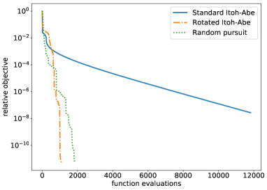
Its global minimiser is located in a narrow, curved valley, which is challenging for the iterates to navigate. We compare the three variants of the Itoh–Abe method, for which we set the algorithm parameters , , , , and . See Figure 6.1 for the numerical results. All three methods converge to the global minimiser, which shows that the Itoh–Abe methods are robust. Unsurprisingly, the random pursuit method and the rotated Itoh–Abe method, which descend in varying directions, perform significantly better than the standard Itoh–Abe method.
We also consider a nonsmooth variant of (6.1), termed Nesterov’s (second) nonsmooth Chebyshev–Rosenbrock function (gur12, ),
| (6.2) |
In this case too, the global minimiser is located along a narrow path. Furthermore, there is a nonminimising, stationary point at , which is nonregular—i.e. it has negative directional derivatives).
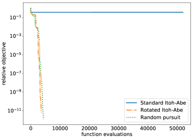
We also compare the three Itoh–Abe methods for this example, and set the algorithm parameters , , , , and . See Figure 6.2 for the results from this. As can be seen, the standard Itoh–Abe discrete gradient method is not suitable for the irregular paths and nonsmooth kinks of the objective function, and stagnates early on. The two randomised Itoh–Abe methods perform better, as they descend in varying directions. For the remaining 2D problems in this paper, we will consider the rotated Itoh–Abe method, although we could just as well have used the random pursuit method. For higher-dimensional problems, we recommend the random pursuit method.
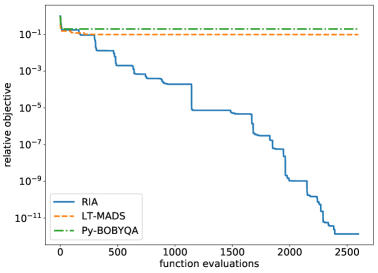
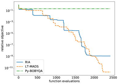
We also compare the performance of the randomised Itoh–Abe (RIA) method to Py-BOBYQA and LT-MADS for Nesterov’s nonsmooth Chebyshev–Rosenbrock function. We set the parameters of the Itoh–Abe method to , , , , and , the parameters of Py-BOBYQA to , and , and the parameters of LT-MADS to and . See Figure 6.3 and 6.4 for the numerical results for two different starting points. In the first case, the Itoh–Abe method successfully converges to the global minimiser, the LT-MADS method locates the nonminimising stationary point at , while the Py-BOBYQA iterates stagnate at a kink, reflecting the fact that the method is not designed for nonsmooth functions. In the second case, both the Itoh–Abe method and LT-MADS locate the minimiser, while the Py-BOBYQA iterates stagnate at a kink.
6.2 Bilevel parameter learning in image analysis
In this subsection, we consider the Itoh–Abe method for solving bilevel optimisation problems for the learning of parameters of variational imaging problems. We restrict our focus to denoising problems, although the same method could be applied to any inverse problem. We first consider one-dimensional bilevel problems with wavelet and TV denoising, and two-dimensional problems with TGV denoising. In the TGV case, we compare the randomised Itoh–Abe method to the Py-BOBYQA and LT-MADS methods. Throughout this section, we set , where .
6.2.1 Setup for variational regularisation problem
Consider an image , for some domain , and a noisy image
To recover a clean image from the noisy one, we consider a parametrised family of regularisers,
and solve the variational regularisation problem
| (6.3) |
The first term in (6.3), the data fidelity term, ensures that the reconstruction approximates . The regulariser term serves to denoise the reconstruction, by promoting favourable features such as smooth regions and sharp edges. The parameters determine how heavily to regularise, and sometimes adjust other features of the regulariser. See (ben18, ; ito14, ; sch08, ) for an overview of variational regularisation methods.
We list some common regularisers in image analysis. Total variation (TV) (bur13, ; rud92, ) is given by the function , where , and
This is one of the most common regularisers for image denoising. See Figure 6.5 for an example of denoising with TV regularisation. We also consider its second-order generalisation, total generalised variation (bre10, ; bre15, ), , where and
For a linear operator on , the basis pursuit regulariser
promotes sparsity of the image in the dictionary of .
As illustrated in Figure 6.5, the quality of the reconstruction is sensitive to . If is too low, the reconstruction is too noisy, while if is too high, too much detail is removed. As it is generally not possible to ascertain the optimal choice of a priori, a significant amount of time and effort is spent on parameter tuning. It is therefore of interest to improve our understanding of optimal parameter choices. One approach is to learn suitable parameters from training data. This requires a desired reconstruction , noisy data , and a scoring function that measures the error between and the reconstruction . The bilevel optimisation problem is given by
| (6.4) |
In our case, we have strong convexity in the data fidelity term, which implies that is unique for each . We can therefore define a mapping
| (6.5) |
The bilevel problem (6.4) is difficult to tackle, both analytically as well as numerically. In most cases, the lower level problem (6.3) does not have a closed form formulation. Instead, a reconstruction is approximated numerically with an algorithm. Therefore, one typically does not have access to gradient or subgradient information555While automatic differentiation (gri08, ) can be useful for these purposes, it is in many cases not applicable to iterative algorithms that involve nonsmooth terms or for which the number of iterations cannot be predetermined. See (nes17, ) for further discussion of why derivative-free optimisation schemes are still needed. for the mappings . Furthermore, the bilevel mapping is often nonsmooth and nonconvex. Therefore, numerically solving (6.4) amounts to solving a nonsmooth, nonconvex function in a blackbox setting. We consider the application of the Itoh–Abe method for these problems.
For the numerical experiments in this paper, we reparametrise as , where the exponential operator is applied elementwise on the parameters. There are two reasons for doing so. The first reason is that this paper is concerned with unconstrained optimisation, and this parametrisation allows is to optimise on instead of . The second reason is that has been found to be a preferable scaling for purposes of numerical optimisation.
6.2.2 Wavelet denoising
We consider the wavelet denoising problem
where is a wavelet transform. In particular, is an orthonormal basis, which implies that the regularisation problem has the unique solution
where is the shrinkage operator defined by
We first optimise for the scoring function
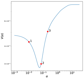
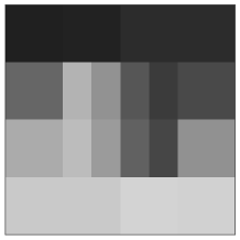
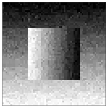
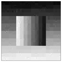
We set the parameters of the Itoh–Abe method to , , , and . See Figure 6.6 for the numerical results.
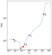

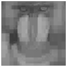


We also optimise with respect to the scoring function , where is the structural similarity function (wan04, )
Here is the mean intensity of , is the unbiased estimate of the standard deviation of , and is the correlation coefficient between and :
We set the parameters of the Itoh–Abe method to , , , and . See Figure 6.7 for the numerical results.


6.2.3 Total variation denoising
We consider the TV denoising problem
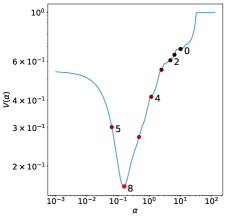
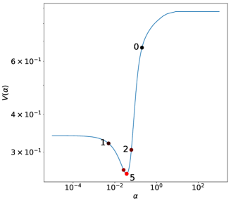
with the SSIM scoring function. We solve the above denoising problem using the PDHG method (cha11, ). We set the parameters of the Itoh–Abe method to , , , and . See Figure 6.8 for the numerical results.
6.2.4 Total generalised variation regularisation
We now consider the second-order total generalised variation (TGV) regulariser for image denoising, with the scoring function
Like for TV denoising, we solve the denoising problem using the PDHG method. We set the parameters of the randomised Itoh–Abe (RIA) method to , , , and . See Figure 6.9 for the numerical results.
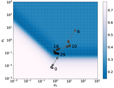
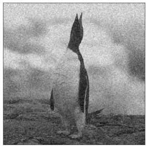


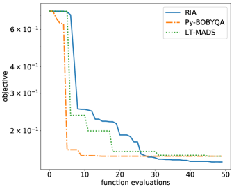
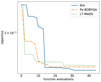
We compare these results to the results from the Py-BOBYQA and LT-MADS solvers. We set the parameters of Py-BOBYQA to , and and the parameters of LT-MADS to . See the results for two different starting points in Figure 6.10 and 6.11. We note that the objective function is approximately stationary across a range of values, which leads to the different points of convergence, and different limiting values of the objective function for different methods. We see that the methods are all of comparable efficiency, although the Itoh–Abe method is slower initially. The Itoh–Abe method seems to be the most efficient, once it is within a neighborhood of the minimiser.
7 Conclusion
In this paper, we have shown that the randomised Itoh–Abe methods are efficient and robust schemes for solving unconstrained nonsmooth, nonconvex problems without the use of gradients or subgradients. Furthermore, the favourable rates of dissipativity that the discrete gradient method inherits from the gradient flow system extends to the nonsmooth case. We show, under minimal assumptions on the objective function, that the methods admit a solution that is computationally tractable, and the iterates converge to a connected set of Clarke stationary points. Through examples, the assumptions are also shown to be necessary.
The methods are shown to be robust and versatile optimisation schemes. It locates the global minimisers of the Rosenbrock function and a variant of Nesterov’s nonsmooth Chebyshev–Rosenbrock functions. The efficiency of the Itoh–Abe discrete gradient method for smooth problems has already been demonstrated elsewhere (gri17, ; miy17, ; rin17, ). We also consider its application to bilevel learning problems and compare its performance to the derivative-free Py-BOBYQA and LT-MADS methods.
Future work will be dedicated to adapting the randomised Itoh–Abe methods for constrained optimisation problems, establishing convergence of the iterates of the method for Kurdyka-Łojasiewicz functions (att10, ), and analysing the Lipschitz continuity properties of bilevel optimisation for variational regularisation problems.
Acknowledgements.
The authors give thanks to Lindon Roberts for helpful discussions and for providing code for Py-BOBYQA, and to Antonin Chambolle for helpful discussions.References
- (1) Attouch, H., Bolte, J., Redont, P., Soubeyran, A.: Proximal alternating minimization and projection methods for nonconvex problems: An approach based on the Kurdyka-Łsojasiewicz inequality. Mathematics of Operations Research 35(2), 438–457 (2010)
- (2) Audet, C., Dennis Jr, J.E.: Mesh adaptive direct search algorithms for constrained optimization. SIAM Journal on optimization 17(1), 188–217 (2006)
- (3) Audet, C., Hare, W.: Derivative-Free and Blackbox Optimization, 1st edn. Springer Series in Operations Research and Financial Engineering. Springer International Publishing (2017)
- (4) Aussel, D.: Subdifferential properties of quasiconvex and pseudoconvex functions: unified approach. Journal of optimization theory and applications 97(1), 29–45 (1998)
- (5) Bagirov, A.M., Karasözen, B., Sezer, M.: Discrete gradient method: derivative-free method for nonsmooth optimization. Journal of Optimization Theory and Applications 137(2), 317–334 (2008)
- (6) Benning, M., Burger, M.: Modern Regularization Methods for Inverse Problems. ArXiv e-prints (2018). URL http://arxiv.org/abs/1801.09922
- (7) Borwein, J.M., Zhu, Q.J.: A survey of subdifferential calculus with applications. Nonlinear Analysis: Theory, Methods & Applications 38(6), 687–773 (1999)
- (8) Bredies, K., Holler, M.: A TGV-based framework for variational image decompression, zooming, and reconstruction. part I: Analytics. SIAM Journal on Imaging Sciences 8(4), 2814–2850 (2015)
- (9) Bredies, K., Kunisch, K., Pock, T.: Total generalized variation. SIAM Journal on Imaging Sciences 3(3), 492–526 (2010)
- (10) Burger, M., Osher, S.: A guide to the TV zoo. In: Level set and PDE based reconstruction methods in imaging, pp. 1–70. Springer, Berlin (2013)
- (11) Burke, J.V., Curtis, F.E., Lewis, A.S., Overton, M.L., Simões, L.E.: Gradient sampling methods for nonsmooth optimization. arXiv e-prints (2018). URL http://arxiv.org/abs/1804.11003
- (12) Calatroni, L., Chung, C., De Los Reyes, J.C., Schönlieb, C.B., Valkonen, T.: Bilevel approaches for learning of variational imaging models. ArXiv e-prints (2015). URL http://arxiv.org/abs/1505.02120
- (13) Cartis, C., Fiala, J., Marteau, B., Roberts, L.: Improving the Flexibility and Robustness of Model-Based Derivative-Free Optimization Solvers. ArXiv e-prints (2018). URL http://arxiv.org/abs/1804.00154
- (14) Chambolle, A., Pock, T.: A first-order primal-dual algorithm for convex problems with applications to imaging. Journal of mathematical imaging and vision 40(1), 120–145 (2011)
- (15) Clarke, F.H.: Necessary conditions for nonsmooth problems in optimal control and the calculus of variations. Ph.D. thesis, University of Washington (1973)
- (16) Clarke, F.H.: Optimization and Nonsmooth Analysis, 1st edn. Classics in Applied Mathematics. SIAM, Philadelphia (1990)
- (17) Curtis, F.E., Que, X.: An adaptive gradient sampling algorithm for non-smooth optimization. Optimization Methods and Software 28(6), 1302–1324 (2013)
- (18) Curtis, F.E., Que, X.: A quasi-Newton algorithm for nonconvex, nonsmooth optimization with global convergence guarantees. Mathematical Programming Computation 7(4), 399–428 (2015)
- (19) DuPont, B., Cagan, J.: A hybrid extended pattern search/genetic algorithm for multi-stage wind farm optimization. Optimization and Engineering 17(1), 77–103 (2016)
- (20) Ehrhardt, M.J., Riis, E.S., Ringholm, T., Schönlieb, C.B.: A geometric integration approach to smooth optimisation: Foundations of the discrete gradient method. ArXiv e-prints (2018). URL http://arxiv.org/abs/1805.06444
- (21) Ekeland, I., Téman, R.: Convex Analysis and Variational Problems, 1st edn. SIAM, Philadelphia, PA, USA (1999)
- (22) Fasano, G., Liuzzi, G., Lucidi, S., Rinaldi, F.: A linesearch-based derivative-free approach for nonsmooth constrained optimization. SIAM Journal on Optimization 24(3), 959–992 (2014)
- (23) Fowler, K.R., Reese, J.P., Kees, C.E., Dennis Jr, J., Kelley, C.T., Miller, C.T., Audet, C., Booker, A.J., Couture, G., Darwin, R.W., et al.: Comparison of derivative-free optimization methods for groundwater supply and hydraulic capture community problems. Advances in Water Resources 31(5), 743–757 (2008)
- (24) Giles, J.R.: A survey of Clarke’s subdifferential and the differentiability of locally Lipschitz functions. In: Progress in Optimization, pp. 3–26. Springer, Boston (1999)
- (25) Gonzalez, O.: Time integration and discrete Hamiltonian systems. Journal of Nonlinear Science 6(5), 449–467 (1996)
- (26) Gray, G.A., Kolda, T.G., Sale, K., Young, M.M.: Optimizing an empirical scoring function for transmembrane protein structure determination. INFORMS Journal on Computing 16(4), 406–418 (2004)
- (27) Griewank, A., Walther, A.: Evaluating Derivatives: Principles and Techniques of Algorithmic Differentiation, 2nd edn. Society for Industrial and Applied Mathematics, Philadelphia (2008)
- (28) Grimm, V., McLachlan, R.I., McLaren, D.I., Quispel, G.R.W., Schönlieb, C.B.: Discrete gradient methods for solving variational image regularisation models. Journal of Physics A: Mathematical and Theoretical 50(29), 295201 (2017)
- (29) Gürbüzbalaban, M., Overton, M.L.: On Nesterov’s nonsmooth Chebyshev–Rosenbrock functions. Nonlinear Analysis: Theory, Methods & Applications 75(3), 1282–1289 (2012)
- (30) Hairer, E., Lubich, C., Wanner, G.: Geometric numerical integration: structure-preserving algorithms for ordinary differential equations, vol. 31, 2nd edn. Springer Science & Business Media, Berlin (2006)
- (31) Heath, M.T.: Scientific Computing: An Introductory Survey, 1st edn. McGraw-Hill, New York (2002)
- (32) Hintermüller, M.: A proximal bundle method based on approximate subgradients. Computational Optimization and Applications 20(3), 245–266 (2001)
- (33) Ito, K., Jin, B.: Inverse Problems: Tikhonov Theory And Algorithms, 1st edn. Series On Applied Mathematics. World Scientific Publishing Company, Singapore (2014)
- (34) Itoh, T., Abe, K.: Hamiltonian-conserving discrete canonical equations based on variational difference quotients. Journal of Computational Physics 76(1), 85–102 (1988)
- (35) Kämpf, J.H., Robinson, D.: Optimisation of building form for solar energy utilisation using constrained evolutionary algorithms. Energy and Buildings 42(6), 807–814 (2010)
- (36) Karimi, H., Nutini, J., Schmidt, M.: Linear convergence of gradient and proximal-gradient methods under the Polyak–Łojasiewicz condition. In: Joint European Conference on Machine Learning and Knowledge Discovery in Databases, pp. 795–811. Springer (2016)
- (37) Kiwiel, K.C.: Methods of descent for nondifferentiable optimization, vol. 1133, 1st edn. Springer, Berlin (1985)
- (38) Kiwiel, K.C.: A nonderivative version of the gradient sampling algorithm for nonsmooth nonconvex optimization. SIAM Journal on Optimization 20(4), 1983–1994 (2010)
- (39) Kunisch, K., Pock, T.: A bilevel optimization approach for parameter learning in variational models. SIAM Journal on Imaging Sciences 6(2), 938–983 (2013)
- (40) Le Digabel, S.: Algorithm 909: NOMAD: Nonlinear optimization with the MADS algorithm. ACM Transactions on Mathematical Software 37(4), 1–15 (2011). URL https://www.gerad.ca/nomad/Project/Home.html
- (41) Le Digabel, S., Tribes, C., Audet, C.: NOMAD user guide. technical report g-2009-37. Tech. rep., Les cahiers du GERAD (2009)
- (42) Lewis, A.S., Overton, M.L.: Nonsmooth optimization via quasi-Newton methods. Mathematical Programming 141, 135–163 (2013)
- (43) Liuzzi, G., Truemper, K.: Parallelized hybrid optimization methods for nonsmooth problems using NOMAD and linesearch. Computational and Applied Mathematics 37, 3172–3207 (2018)
- (44) Martin, D., Fowlkes, C., Tal, D., Malik, J.: A database of human segmented natural images and its application to evaluating segmentation algorithms and measuring ecological statistics. In: Proceedings of the 8th International Conference on Computer Vision, vol. 2, pp. 416–423. IEEE (2001)
- (45) McLachlan, R.I., Quispel, G.R.W.: Six lectures on the geometric integration of ODEs, p. 155–210. London Mathematical Society Lecture Note Series. Cambridge University Press, Cambridge (2001)
- (46) McLachlan, R.I., Quispel, G.R.W., Robidoux, N.: Geometric integration using discrete gradients. Philosophical Transactions of the Royal Society of London A: Mathematical, Physical and Engineering Sciences 357(1754), 1021–1045 (1999)
- (47) Michel, P., Penot, J.P.: Calcul sous-différentiel pour des fonctions lipschitziennes et non lipschitziennes. C. R. Acad. Sci. Paris 1, 269–272 (1984)
- (48) Miyatake, Y., Sogabe, T., Zhang, S.L.: On the equivalence between SOR-type methods for linear systems and discrete gradient methods for gradient systems. ArXiv e-prints (2017). URL http://arxiv.org/abs/1711.02277
- (49) Nelder, J.A., Mead, R.: A simplex method for function minimization. The computer journal 7(4), 308–313 (1965)
- (50) Nesterov, Y., Spokoiny, V.: Random gradient-free minimization of convex functions. Foundations of Computational Mathematics 17(2), 527–566 (2017)
- (51) Ochs, P., Ranftl, R., Brox, T., Pock, T.: Bilevel optimization with nonsmooth lower level problems. In: International Conference on Scale Space and Variational Methods in Computer Vision, pp. 654–665. Springer (2015)
- (52) Oeuvray, R., Bierlaire, M.: A new derivative-free algorithm for the medical image registration problem. International Journal of Modelling and Simulation 27(2), 115–124 (2007)
- (53) Penot, J.P., Quang, P.H.: Generalized convexity of functions and generalized monotonicity of set-valued maps. Journal of Optimization Theory and Applications 92(2), 343–356 (1997)
- (54) Polyak, B.T.: Introduction to Optimization, 1st edn. Optimization Software, Inc., New York (1987)
- (55) Powell, M.J.D.: The NEWUOA software for unconstrained optimization without derivatives. In: Large-scale nonlinear optimization, 1st edn., pp. 255–297. Springer, Boston (2006)
- (56) Powell, M.J.D.: The BOBYQA algorithm for bound constrained optimization without derivatives. Tech. rep., University of Cambridge (2009)
- (57) Quispel, G.R.W., Turner, G.S.: Discrete gradient methods for solving ODEs numerically while preserving a first integral. Journal of Physics A: Mathematical and General 29(13), 341–349 (1996)
- (58) De los Reyes, J.C., Schönlieb, C.B., Valkonen, T.: Bilevel parameter learning for higher-order total variation regularisation models. Journal of Mathematical Imaging and Vision 57(1), 1–25 (2017)
- (59) Ringholm, T., Lazić, J., Schönlieb, C.B.: Variational image regularization with Euler’s elastica using a discrete gradient scheme. ArXiv e-prints (2017). URL http://arxiv.org/abs/1712.07386
- (60) Rosenbrock, H.H.: An automatic method for finding the greatest or least value of a function. The Computer Journal 3(3), 175–184 (1960)
- (61) Rudin, L.I., Osher, S., Fatemi, E.: Nonlinear total variation based noise removal algorithms. Physica D: nonlinear phenomena 60(1-4), 259–268 (1992)
- (62) Rudin, W.: Principles of Mathematical Analysis, 3rd edn. International series in pure and applied mathematics. McGraw-Hill, New York (1976)
- (63) Scherzer, O., Grasmair, M., Grossauer, H., Haltmeier, M., Lenzen, F.: Variational Methods in Imaging, 1st edn. Applied Mathematical Sciences. Springer, New York (2008)
- (64) Wang, Z., Bovik, A.C., Sheikh, H.R., Simoncelli, E.P.: Image quality assessment: from error visibility to structural similarity. IEEE transactions on image processing 13(4), 600–612 (2004)