Learning Hybrid Sparsity Prior for Image Restoration: Where Deep Learning Meets Sparse Coding

Abstract

State-of-the-art approaches toward image restoration can be classified into model-based and learning-based. The former - best represented by sparse coding techniques - strive to exploit intrinsic prior knowledge about the unknown high-resolution images; while the latter - popularized by recently developed deep learning techniques - leverage external image prior from some training dataset. It is natural to explore their middle ground and pursue a hybrid image prior capable of achieving the best in both worlds. In this paper, we propose a systematic approach of achieving this goal called Structured Analysis Sparse Coding (SASC). Specifically, a structured sparse prior is learned from extrinsic training data via a deep convolutional neural network (in a similar way to previous learning-based approaches); meantime another structured sparse prior is internally estimated from the input observation image (similar to previous model-based approaches). Two structured sparse priors will then be combined to produce a hybrid prior incorporating the knowledge from both domains. To manage the computational complexity, we have developed a novel framework of implementing hybrid structured sparse coding processes by deep convolutional neural networks. Experimental results show that the proposed hybrid image restoration method performs comparably with and often better than the current state-of-the-art techniques.

I Introduction

Image restoration refers to a class of ill-posed inverse problems recovering unknown images from their degraded observations (e.g., noisy, blurred or down-sampled). It is well known image prior (a.k.a. regularization) plays an important role in the development of solution algorithms to ill-posed image restoration problems. Depending on the availability of training data, one can obtain image prior by either model-based or learning-based approaches. In model-based approaches, image prior is obtained by mathematical construction of a penalty functional (e.g., total-variation or sparse coding) and its parameters have to be intrinsically estimated from the observation data; in learning-based approaches, image prior is leveraged externally from training data - e.g., a deep convolutional neural network is trained to learn the mapping from the space of degraded images to that of restored ones. We will briefly review the key advances within each paradigm in the past decade, which serves as the motivation for developing a hybrid (internal+external) prior in this work.

In model-based approaches, sparse coding and its variations are likely to be the most studied in the literature [1, 2, 3, 4, 5, 6, 7, 8, 9, 10, 11, 12, 13, 14, 15]. The basic idea behind sparse coding is that natural images admit sparse representations in a transformed space. Early works in sparse coding have focused on the characterization of localized structures or transient events in natural images; to obtain basis functions with good localization properties in both spatial and frequency domains, one can either construct them through mathematical design (e.g., wavelet [16]) or learn them from training data (e.g., dictionary learning [17]). Later on the importance of exploiting nonlocal similarity in natural images (e.g., self-repeating patterns in textured regions) was recognized in a flurry of so-called simultaneous sparse coding works including BM3D [18] and LSSC [19] as well as nonlocal sparsity based image restoration [5, 6, 7]. Most recently, nonlocal sparsity has been connected with the powerful Gaussian scalar mixture (GSM) model [20] leading to the state-of-the-art performance in image restoration [21].

In learning-based approaches, deep neural network (DNN) techniques have attracted increasingly more attention and shown significant improvements in various low-level vision applications including superresolution (SR) and restoration [10, 13, 14, 12, 22, 23]. In [24], stacked collaborative auto-encoders are used to gradually recover a high-resolution (HR) image layer by layer; in [11], a SR method using predictive convolutional sparse coding and deconvolution network was developed. Multiple convolutional neural network [10, 13, 14] have been proposed to directly learn the nonlinear mapping between low-resolution (LR) and high-resolution (HR) images; and multi-stage trainable nonlinear reaction diffusion network has also been proposed for image restoration [25]. Moreover, most recent studies have shown that deeper neural network can lead to even better SR performance [13, 14]. However, it should be noted that the DNN approach [10, 13, 14] still performs poorly on some particular sample images (e.g., if certain texture information is absent in the training data). Such mismatch between training and testing data is a fundamental limitation of all learning-based approaches.

One possible remedy for overcoming the above limitation is to explore somewhere between - i.e., a hybrid approach combining the best of both worlds. Since training data and degraded image respectively contain supplementary (external and internal) prior information, it is natural to combine them for image restoration. The key challenge is how to pursue such a hybrid approach in a principled manner. Inspired by the previous work connecting DNN with sparse coding (e.g., [26] and [12]), we propose a Structured Analysis Sparse Coding (SASC) framework to jointly exploit the prior in both external and internal sources. Specifically, an external structured sparse prior is learned from training data via a deep convolutional neural network (in a similar way to previous learning-based approaches); meantime another internal structured sparse prior is estimated from the degraded image (similar to previous model-based approaches). Two structured sparse priors will be combined to produce a hybrid prior incorporating the knowledge from both domains. To manage the computational complexity, we have developed a novel framework of implementing hybrid structured sparse coding processes by deep convolutional neural networks. Experimental results have shown that the proposed hybrid image restoration method performs comparably with and often better than the current state-of-the-art techniques.

II Related Work

II-A Sparse models for image restoration

Generally speaking, sparse models can be classified into synthesis models and analysis models [27]. Synthesis sparse models assume that image patches can be represented as linear combinations of a few atoms from a dictionary. Let $\bm{y}=\textbf{H}\bm{x}+\bm{n}$ denote the degraded image, where $\textbf{H}\in\mathbb{R}^{N\times M}$ is the observation matrix (e.g. blurring and down-sampling) and $\bm{n}\in\mathbb{R}^{N}$ is the additive Gaussian noise. Then synthesis sparse model based image restoration can be formulated as Eq. (1)

$$(\bm{x},\bm{\alpha}_{i})=\operatorname*{argmin}_{\bm{x},\bm{\alpha}_{i}}||\bm{y}-\textbf{H}\bm{x}||_{2}^{2}+\eta\sum_{i}\{||\textbf{R}_{i}\bm{x}-\textbf{D}\bm{\alpha}_{i}||_{2}^{2}+\lambda||\bm{\alpha}_{i}||_{1}\},$$ (1)

where $\textbf{R}_{i}$ denote the matrix extracting patches of size $\sqrt{n}\times\sqrt{n}$ at position $i$ and $\textbf{D}\in\mathbb{R}^{n\times K}$ is the dictionary. The above optimization problem can be solved by alternatively optimizing $\bm{\alpha}_{i}$ and $\bm{x}$. The $\ell_{1}$ norm minimization problem in Eq. (1) requires many iterations and is typically computational expensive.

Alternatively, analysis sparse model (ASC) [27] assumes that image patches are sparse in a transform domain- i.e., for a given dictionary $\textbf{W}\in\mathbb{R}^{K\times n}$ of analysis, $||\textbf{W}\bm{x}_{i}||_{0}\ll K$ is sparse. With the ASC model, the unknown image can be recovered by solving

$$(\bm{x},\bm{\alpha}_{i})=\operatorname*{argmin}_{\bm{x},\bm{\alpha}_{i}} ||\bm{y}-\textbf{H}\bm{x}||_{2}^{2}+$$

$$\eta\sum_{i}\{||\textbf{W}(\textbf{R}_{i}\bm{x})-\bm{\alpha}_{i}||_{2}^{2}+\lambda||\bm{\alpha}_{i}||_{1}\}.$$ (2)

Note that if image patches are extracted with maximum overlapping along both horizontal and vertical directions, the transformation of each patches can be implemented by the convolution with the set of filters $\bm{w}_{k},k=1,2,\cdots,K$ with $\bm{x}$- i.e.,

$$(\bm{x},\bm{z}_{k})=\operatorname*{argmin}_{\bm{x},\bm{z}_{k}} ||\bm{y}-\textbf{H}\bm{x}||_{2}^{2}+$$

$$\eta\sum_{k=1}^{K}\{||\bm{w}_{k}*\bm{x}-\bm{z}_{k}||_{2}^{2}+\lambda||\bm{z}_{k}||_{1}\}.$$ (3)

$z_{k}$ represents sparse feature map corresponding to filter $w_{k}$. Compared with the synthesis sparse model, sparse codes or feature maps in Eq. (2) and (3) can be solved in a closed-form solution, leading to significant reduction in computational complexity.

II-B Connecting sparsity with neural networks

Recent studies have shown that sparse coding problem can be approximately solved by a neural network [26]. In [26], a feed-forward neural network, which mimics the process of sparse coding, is proposed to approximate the sparse codes $\bm{\alpha}_{i}$ with respect to a given synthesis dictionary D. By joint learning all model parameters from training dataset, good approximation of the underlying sparse codes can be obtained. In [12], the connection between sparse coding and neural networks has been further extended for the application of image SR. Sparse coding (SC) based neural network is designed to emulate sparse coding based SR process - i.e., sparse codes of LR patches are first approximated by a neural network and then used to reconstruct HR patches with a HR synthesis dictionary. By jointly training all model parameters, SC-based neural network can achieve much better results than conventional SC-based methods. The fruitful connection between sparse coding and neural networks also inspires us to combine them in a more principled manner in this paper.

III Structured analysis sparse coding (SASC) for image restoration

The analysis SC model of Eq. (2) and (3) has the advantage of computational efficiency when compared to the synthesis SC model. However, $\ell_{1}$-norm based SC model ignores the correlation among sparse coefficients, leading to unsatisfactory results. Similar to previous works of nonlocal sparsity [6, 7], a structured ASC model for image restoration can be formulated as

$$(\bm{x},\bm{z}_{k})=\operatorname*{argmin}_{\bm{x},\bm{z}_{k}} ||\bm{y}-\textbf{H}\bm{x}||_{2}^{2}+$$

$$\eta\sum_{k=1}^{K}\{||\bm{w}_{k}*\bm{x}-\bm{z}_{k}||_{2}^{2}+\lambda||\bm{z}_{k}-\bm{\mu}_{k}||_{1}\},$$ (4)

where $\bm{\mu}_{k}$ denotes the new nonlocal prior of the feature map (note that when $\bm{\mu}_{k}=\bm{0}$ the structured ASC model reduces to the conventional ASC model in Eq. (3)). The introduction of $\bm{\mu}_{k}$ to sparse prior has the potential of leading to significant improvement of the estimation of sparse feature map $\bm{z}_{k}$, which bridges the two competing approaches (model-based vs. learning-based).

The objective function of Eq. (4) can be solved by alternatively optimizing $\bm{x}$ and $\bm{z}_{k}$. With fixed feature maps $\bm{z}_{k}$, the restored image $\bm{x}$ can be updated by computing

$$\bm{x}=(\textbf{H}^{\top}\textbf{H}+\eta\sum_{k}\textbf{W}_{k}^{\top}\textbf{W}_{k})^{-1}(\textbf{H}^{\top}\bm{y}+\eta\sum_{k}\textbf{W}_{k}^{\top}\bm{z}_{k}),$$ (5)

where $\textbf{W}_{k}\bm{x}=\bm{w}_{k}*\bm{x}$ denotes the 2D convolution with filter $\bm{w}_{k}$. Since the matrix to be inverted in Eq. (5) is very large, it is impossible to compute Eq. (5) directly. Instead, it can be computed by the iterative conjugated gradient (CG) algorithm, which requires many iterations. Here, instead of computing an exact solution of the $\bm{x}$-subproblem, we propose to update $\bm{x}$ with a single step of gradient descent of the objective function for an inexact solution, as

$$\begin{split}\bm{x}^{(t+1)}&=\bm{x}^{(t)}-\delta[\textbf{H}^{\top}(\textbf{H}\bm{x}^{(t)}-\bm{y})+\eta\sum_{k}\textbf{W}_{k}^{\top}(\textbf{W}_{k}\bm{x}^{(t)}-\bm{z}_{k})]\\ &=\textbf{A}\bm{x}^{(t)}+\delta\textbf{H}^{\top}\bm{y}+\delta\eta\sum_{k}\textbf{W}_{k}^{\top}\bm{z}_{k},\end{split}$$ (6)

where $\textbf{A}=\textbf{I}-\delta\textbf{H}^{\top}\textbf{H}-\delta\eta\sum_{k}\textbf{W}_{k}^{\top}\textbf{W}_{k}$, $\delta$ is the predefined step size, and $\bm{x}^{(t)}$ denotes the estimate of the whole image $\bm{x}$ at the $t$-th iteration. As will be shown later, the update of $\bm{x}^{(t)}$ can be efficiently implemented by convolutional operations. With fixed $\bm{x}$, the feature maps can be updated via

$$\bm{z}_{k}=\mathcal{S}_{\lambda/2}(\bm{w}_{k}*\bm{x}-\bm{\mu}_{k})+\bm{\mu}_{k},$$ (7)

where $\mathcal{S}_{\lambda}(\cdot)$ denotes the soft-thresholding operator with a threshold of $\lambda$. Now the question boils down tos how to accurately estimate $\bm{\mu}_{k}$. In the following subsections, we propose to learn the structured sparse prior from both training data (external) and the degraded image (internal).

III-A Prior learning from training dataset

For a given observation image $\bm{y}$, we target at learning the feature maps $\bm{z}_{k}$ of a desirable restored image $\bm{x}$ with respect to filters $\bm{w}_{k}$. Without the loss of generality, the learning function can be defined as follows

$$\hat{\textbf{Z}}=G(\bm{y};\mathbf{\Theta}),$$ (8)

where $\hat{\textbf{Z}}=[\hat{\bm{z}}_{1},\hat{\bm{z}}_{2},\cdots,\hat{\bm{z}}_{K}]$ and $G(\cdot)$ denotes the learning function parameterized by $\mathbf{\Theta}$. Considering the strong representing abilities of convolutional neural networks (CNN), we choose to learn $\bm{z}_{k}$ on a deep CNN (DCNN). We have found that directly learning a set of feature maps $\bm{z}_{k}$ with respect to $\bm{w}_{k}$ is unstable; instead, we propose to first learn the desirable restored image $\hat{\bm{x}}$ and then compute the feature maps via $\hat{\bm{z}}_{k}=\bm{w}_{k}*\hat{\bm{x}}$. Generally speaking, any existing DCNN can be used for an initial estimate of $\bm{x}$. The architecture of DCNN (as shown in Fig. 1) is similar to that of [10]. However, different from [10], convolution filters of smaller size and more convolution layers are used for better estimation performance. The CNN contains $12$ convolution layer, each of which uses 64 filters sized by $3\times 3\times 64$. The last layer uses a single filter of size $3\times 3$ for reconstruction. A shortcut or skip connection (not shown in the figure) exists from input to output implementing the concept of deep residue learning (similar to [14]). The objective function of DCNN training can be formulated as

$$\mathbf{\Theta}=\operatorname*{argmin}_{\mathbf{\Theta}}\sum_{i}||CNN(\bm{y}_{i};\mathbf{\Theta})-\bm{x}_{i}||_{2}^{2}$$ (9)

where $\bm{y}_{i}$ and $\bm{x}_{i}$ denotes the observed and target training image pairs and $CNN(\bm{y}_{i};\mathbf{\Theta})$ denotes the output of CNN with parameters $\mathbf{\Theta}$. All network parameters are optimized through the back-propagation algorithm. After the estimation of $\bm{x}$, the set of feature maps can be estimated by convoluting it with a set of analysis filters $\bm{w}_{k}$- i.e., $\hat{\bm{z}_{k}}=\bm{w}_{k}*\hat{\bm{x}},k=1,2,\cdots,K$.

Figure 1: The structure of the CNN for prior learning. The CNN contains 11 convolution layer with ReLu nonlinear activation function. For each convolution layer, 64 filters of size $3\times 3$ are used. The degraded image is fed into the network to get an initial estimate of the original image.

III-B Prior learning by exploiting nonlocal self-similarity

In addition to externally learning the prior feature maps via CNN, we can also obtain the estimates of $\bm{z}_{k}$ from an internal estimate of the target image. Let $\hat{\bm{x}}_{i}$ denote the patch of size $\sqrt{n}\times\sqrt{n}$ extracted at position $i$ from an initial estimate $\hat{\bm{x}}$; then sparse codes of $\hat{\bm{x}}_{i}$ can be computed as $\hat{\bm{z}}_{i,k}=\bm{w}_{k}^{\top}\hat{\bm{x}}_{i}$. Considering that the natural images contain rich self-repetitive patterns, a better estimate of $\bm{z}_{i,k}$ can be obtained by a weighted average of the sparse codes over similar patches. Let $\hat{\bm{x}}_{i_{l}},l=1,2,\cdots,L$ denote the set of similar patches that are within the first $L$-th closest matches and $G_{i}={i_{1},i_{2}\cdots,i_{L}}$ denote the collection of the positions corresponding to those similar patches. A nonlocal estimate of $\hat{\bm{z}}_{i,k}$ can be calculated as

$$\tilde{\bm{z}}_{i,k}=\sum_{l=1}^{L}w_{i_{l}}\bm{w}_{k}^{\top}\hat{\bm{x}}_{i_{l}}=\bm{w}_{k}^{\top}\tilde{\bm{x}}_{i},$$ (10)

where $w_{i_{l}}=\frac{1}{c}\exp(-||\hat{\bm{x}}_{i_{l}}-\hat{\bm{x}}_{i}||/h)$, $c$ is the normalization constant, $h$ is the predefined constant, and $\tilde{\bm{x}}_{i}=\sum_{l=1}^{L}w_{i_{l}}\hat{\bm{x}}_{i_{l}}$. From Eq. (10), we can see that a nonlocal estimate of the sparse codes can be obtained by first computing the nonlocal estimate of the target image followed by a 2D convolution with the filters $\bm{w}_{k}$.

By combining the estimate obtained by CNN and nonlocal estimation, an improved hybrid prior of the feature maps can be obtained by

$$\bm{\mu}_{k}=\delta\hat{\bm{z}}_{k}+(1-\delta)\tilde{\bm{z}}_{k},$$ (11)

where $0<\delta<1$ is a preselected constant. The overall structured analysis sparse coding (SASC) with prior learning for image restoration is summarized in Algorithm 1. We note that Algorithm 1 usually requires dozens of iterations for converging to a satisfactory result. Hence, the computational cost of the proposed SASC model is high; meanwhile, the analysis filters $\bm{w}_{k}$ used in Algorithm 1 are kept fixed. A more computationally efficient implementation is to approximate the proposed SASC model by a deep neural network. Through end-to-end training, we can jointly optimize the parameters $\eta$, $\lambda$ and the analysis filters $\bm{w}_{k}$ as will be elaborated next.

Initialization:

• Set parameters $\eta$ and $\lambda$;

• Compute the initial estimate $\hat{\bm{x}}^{(0)}$ by the CNN;

• Group a set of similar patches $G_{i}$ for each patch $\hat{\bm{x}}_{i}$ using $\hat{\bm{x}}^{(0)}$;

• Compute the prior feature maps $\bm{\mu}_{k}$ using Eq. (11);

Outer loop: Iteration over $t=1,2,\cdots,T$

• Compute the feature maps $\bm{z}_{k}^{(t)},k=1,\cdots,K$ using Eq. (7);

• Update the HR image $\hat{\bm{x}}^{(t)}$ via Eq. (6);

• Update $\bm{\mu}_{k}$ via Eq. (11) based on $\hat{\bm{x}}^{(t)}$;

Output: $\bm{x}^{(t)}$.

Algorithm 1 Image SR with structured ASC

IV Network implementation of SASC for image restoration

Figure 2: The structure of the proposed SASC network for image restoration. The whole architecture consists of CNN sub-network and SASC sub-network. Degraded image or intermediate result combine with CNN estimates, feed into multiple SASC recurrent stages to get the final reconstructed image.

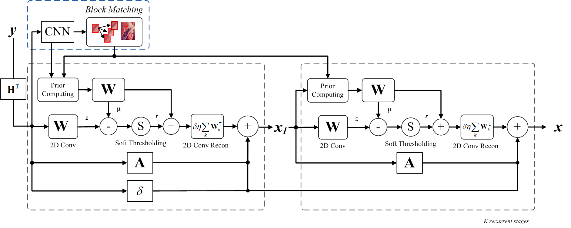
The main architecture for network implementation of SASC is shown in Fig. (2), which mimics the iterative steps of Algorithm 1. As shown in Fig. (2), the degraded observation image $\bm{y}$ goes through the CNN for an initial estimate of the target image, which will then be used for grouping similar patches and computing prior feature maps. Let $G_{i}$ denote the set of similar patch positions for each exemplar patch $\hat{\bm{x}}_{i}$ (for computational simplicity, $G_{i}$ will not be updated during the iterative processing).

The initial estimate obtained via CNN and the set of similar patch positions $G_{i}$ are then fed into the SASC network that contains $k$ recurrent stages to reconstruct the target image. The SASC network exactly mimics the process of alternatively updating of the feature maps $\bm{z}_{k}$ and the HR image $\bm{x}$ as shown in Eq. (7) and (6). The degraded image $\bm{y}$ (after bicubic interpolation if down-sampling is involved) first goes through a convolution layer for sparse feature maps $\bm{z}_{k}$, which will then be predicted by the learned prior feature maps $\bm{\mu}_{k}$. The residuals of the predicted feature maps, denoted by $\bm{r}_{k}$, will go through a nonlinear soft-thresholding layer. Similar to [12], we can write the soft-thresholding operator as

$$s_{\tau_{i}}(r_{i})=\text{Sign}(r_{i})r_{i}(|r_{i}|/\tau_{i}-1)_{+},$$ (12)

where $\tau_{i}$ denotes a tunable threshold. Note that the soft-thresholding layer can be implemented as two linear layers and a unit-threshold layer. After soft-thresholding layer, the learned prior feature maps $\bm{\mu}_{k}$ are added back to the output of soft-thresholding layer. The updated feature maps $\bm{z}_{k}$ then go through a reconstruction layer with a set of 2D convolution filters- i.e., $\sum_{k}\textbf{W}_{k}^{\top}\bm{z}_{k}$. The final output of the reconstruction layer is further added with the preprocessed degraded image- i.e., denoted as $\textbf{H}^{\top}\bm{y}$. Finally, the weighted intermediate result of reconstructed HR image is fed into a linear layer parameterized by matrix A. Note that A corresponds to the matrix - i.e.,

$$\textbf{A}=\textbf{I}-\delta\textbf{H}^{\top}\textbf{H}-\delta\eta\sum_{k}\textbf{W}_{k}^{\top}\textbf{W}_{k}.$$ (13)

Note that $\sum_{k}(\textbf{W}_{k}^{\top}\textbf{W}_{k}\bm{x})$ can be efficiently computed by first convoluting $\bm{x}$ with 2D filters and adding up the resulting feature maps - i.e., $\sum_{k}(\bm{w}_{k}^{\top}*(\bm{w}_{k}*\bm{x}))$. For typical degradation matrices H, $\bar{\textbf{H}}=\textbf{H}^{\top}\textbf{H}$ can also be efficiently computed by convolutional operations. For image denoising, $\bar{\textbf{H}}=\textbf{I}$. For image deblurring, the matrix-vector multiplication $\textbf{H}^{\top}(\textbf{H}\bm{x})$ can be simply implemented by two convolutional operations. For image super-resolution, we consider two typical downsampling operators, i.e., the Gaussian downsampling and the bicubic downsampling. For Gaussian downsampling, H=DB, where D and B denote the downsampling and Gaussian blur matrices, respectively. In this case, $\bm{y}=\textbf{H}\bm{x}$ can be efficiently computed by first convoluting $\bm{x}$ with the corresponding Gaussian filter followed by subsampling, whereas $\textbf{H}^{\top}\bm{y}$ can also be efficiently computed by first upsampling $\bm{y}$ with zero-padding followed by convolution with the transposed Gaussian filter. For bicubic downsampling, we simply use the bicubic interpolator function with scaling factor $s$ and $1/s$ ($s=2,3,4$) to implement $\textbf{H}^{\top}\bm{y}$ and $\textbf{H}\bm{x}$, respectively. Note that all convolutional filters and the scale variables involved in the linear layer A can be discriminately learned through end-to-end training. After going through the linear A, we obtain the reconstructed image; for better performance, such SASC sub-network can be repeated $K$ times.

In summary, there are totally $5$ trainable layers in each stage of our proposed network: two convolution layers W, one reconstruction layer parameterized with $\sum_{k}\textbf{W}_{k}^{\top}\bm{z}_{k}$, one nonlinear soft-thresholding layer, and one linear layer A. Parameters at different stages are not same; but the $i$-th stage of diffenent networks share the same weights $W^{(i)}$. Mean square error is used as the cost function to train the network, and the overall objective function is given by

$$\mathbf{\Theta}=\operatorname*{argmin}_{\mathbf{\Theta}}\sum_{i}||SASC(\bm{y}_{i};\mathbf{\Theta})-\bm{x}_{i}||_{2}^{2}$$ (14)

where $\mathbf{\Theta}$ denotes the set of parameters and $SASC(\bm{y}_{i};\mathbf{\Theta})$ denotes the reconstructed image by the network with parameters $\mathbf{\Theta}$. To train the network, the ADAM optimizer with setting $\beta_{1}=0.9$ and $\beta_{2}=0.999$ and $\epsilon=10^{-8}$ is used. Note that to facilitate training, we separately train the CNN network and the SASC network. Some examples of the learned convolution filters are shown in Fig. (3).

Figure 3: Visualization of some of the learned analysis filters in first SASC stage. It can be infer from this figure that the filters has different responses to the edge features of different directions and frequencies.

V Experimental results

To verify the performance of the proposed method, several image restoration experiments have been conducted, including denoising, deblurring and super-resolution. In all experiments, we empirically set $K=5$ stages for the proposed SASC network. To gain deeper insight toward the proposed SASC network, we have implemented several variants of the proposed SASC network. The first variant is the analysis sparse coding (ASC) network without CNN and self-similarity prior learning. The second variant of the proposed method is the SASC network with self-similarity prior, which estimate $\bm{\mu}_{k}$ from intermediately recovered HR image (without using CNN sub-network), which is denoted as SASC-SS method. We also present the image restoration results of the CNN sub-network, which consists of 12 convolutional layers with ReLU nonlinearity and $3\times 3\times 64$ kernels. The proposed SASC network with CNN and self-similarity prior learning is denoted as SASC-CNN-SS method. To train the networks, we have adopted three training sets: the train400 dataset used in [28] for image denoising/deblurring, the 91 training images used in [3] and the BSD200 dataset for image super-resolution.

V-A Image denoising

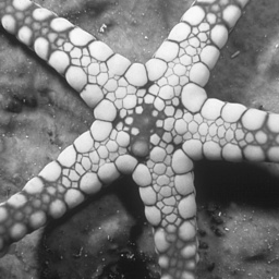
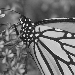
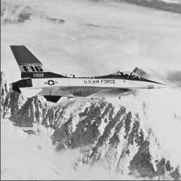
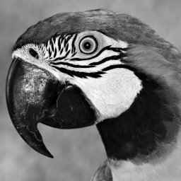
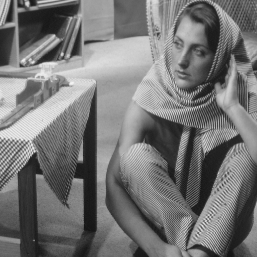
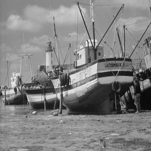
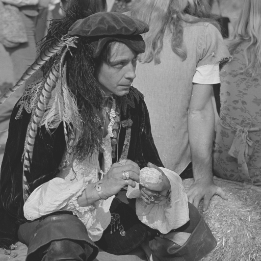
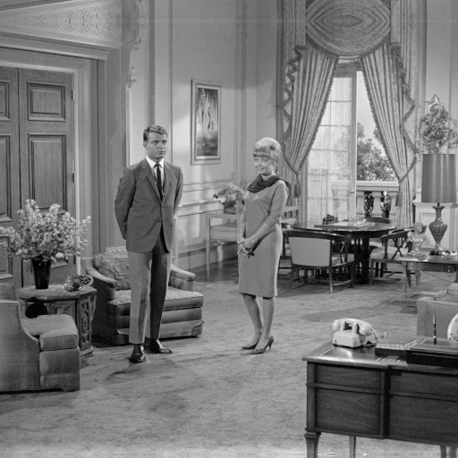
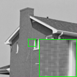
In our experiment, we have extracted patches of size $40\times 40$ from the train400 dataset [28] and used argumentation with flip and rotations to generate $6000\times 128$ patches as the training data. The commonly used $12$ images used in [29] (as shown in Fig. 4) were used as the test set. The BSD68 dataset was also used as a benchmark dataset. The average PSNR and SSIM results of the variants of the proposed SASC methods on the two sets are shown in Table I. From Table I, one can see that by incorporating the nonlocal self-similarity prior, the SASC-SS method outperforms the ASC method; by integrating both CNN (external) and nonlocal self-similarity (internal) priors, the proposed SASC-CNN-SS method further improves the denoising performance. Similar observations have also been made for image deblurring and super-resolution. Due to the limited page spaces, here we only show the comparison studies of the variants of the proposed method for image denoising.

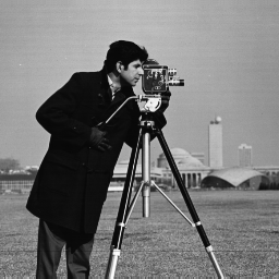
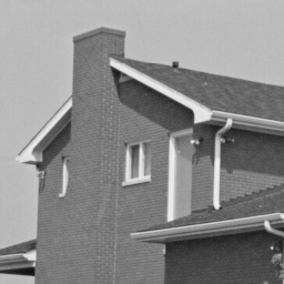
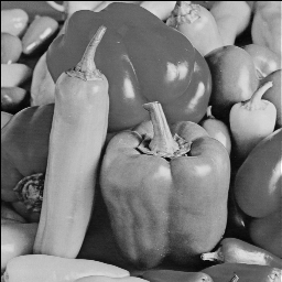
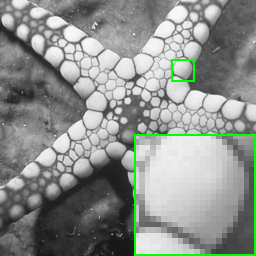
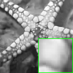
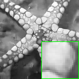
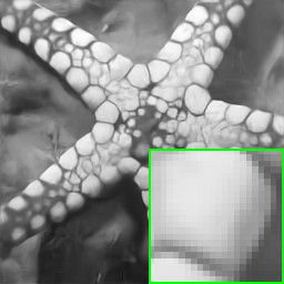
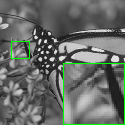
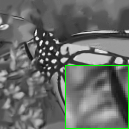
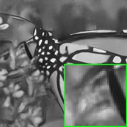
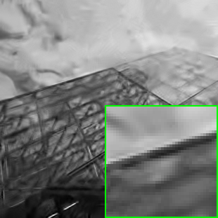
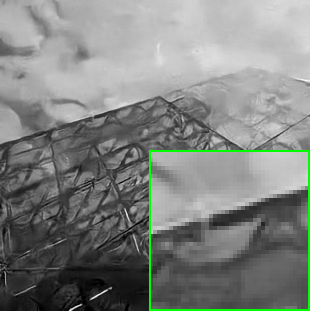
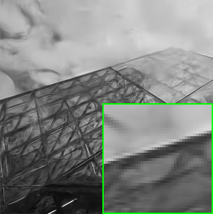
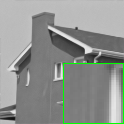
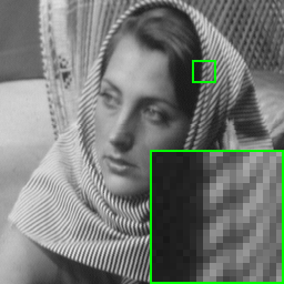
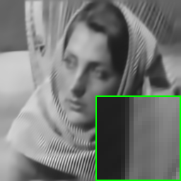
We have also compared the proposed method with several popular denoising methods including model-based denoising methods (BM3D[29], EPLL[30], and WNNM [31]) and two deep learning based methods (TNRD [32] and DnCNN-S[28]). Table II shows the PSNR results of the competing methods on 12 test images. It can be seen that the proposed method performs much better than other competing methods. Specifically, the proposed method outperforms current state-of-the-art DnCNN-S [28] by up to $0.56dB$ on the average. Parts of the denoised images by different methods are shown in Figs. 5-7. It can be seen that the proposed method produces better visually pleasant results, as can be clearly observed in the regions of self-repeating patterns (edges and textures).

Figure 4: The test images used for image denoising/deblurring. From left to right: C.Man, House, Peppers, Starfish, Monarch, Airplane, Parrot, Lena, Barbara, Boat, Man, and Couple.

TABLE I: Average PSNR and SSIM results of the variants of the proposed denoising method

	Set12			BSD68
	$\sigma=15$	$\sigma=25$	$\sigma=50$	$\sigma=15$	$\sigma=25$	$\sigma=50$
ASC	32.60 0.8928	30.30 0.8470	27.01 0.7400	31.65 0.8825	29.11 0.8097	26.01 0.6704
SASC-SS	32.98 0.9016	30.57 0.8601	27.35 0.7669	31.88 0.8888	29.36 0.8243	26.34 0.7006
CNN-Prior	32.85 0.8897	30.38 0.8394	27.24 0.7611	31.75 0.8839	29.17 0.8115	26.23 0.6924
SASC-CNN-SS	33.32 0.9039	30.99 0.8673	27.69 0.7915	32.03 0.8870	29.63 0.8289	26.66 0.7254

TABLE II: Results of proposed denoising method in Set12

IMAGE	C.Man	House	Peppers	Starfish	Monar	Airpl	Parrot	Lena	Barbara	Boat	Man	Couple	Avg
Noise Lv	$\sigma=15$
[29]	31.92	34.94	32.70	31.15	31.86	31.08	31.38	34.27	33.11	32.14	31.93	32.11	32.38
[31]	32.18	35.15	32.97	31.83	32.72	31.40	31.61	34.38	33.61	32.28	32.12	32.18	32.70
[30]	31.82	34.14	32.58	31.08	32.03	31.16	31.40	33.87	31.34	31.91	31.97	31.90	32.10
[32]	32.19	34.55	33.03	31.76	32.57	31.47	31.63	34.25	32.14	32.15	32.24	32.11	32.51
[28]	32.62	35.00	33.29	32.23	33.10	31.70	31.84	34.63	32.65	32.42	32.47	32.47	32.87
Ours	32.16	35.51	33.87	32.67	33.30	31.98	32.21	35.19	33.92	32.99	32.93	33.08	33.31
Noise Lv	$\sigma=25$
[29]	29.45	32.86	30.16	28.56	29.25	28.43	28.93	32.08	30.72	29.91	29.62	29.72	29.98
[31]	29.64	33.23	30.40	29.03	29.85	28.69	29.12	32.24	31.24	30.03	29.77	29.82	30.26
[30]	29.24	32.04	30.07	28.43	29.30	28.56	28.91	31.62	28.55	29.69	29.63	29.48	29.63
[32]	29.71	32.54	30.55	29.02	29.86	28.89	29.18	32.00	29.41	29.92	29.88	29.71	30.06
[28]	30.19	33.09	30.85	29.40	30.23	29.13	29.42	32.45	30.01	30.22	30.11	30.12	30.43
Ours	29.82	33.82	31.47	30.10	30.67	29.50	29.87	33.09	31.32	30.86	30.64	30.77	30.99
Noise Lv	$\sigma=50$
[29]	26.13	29.69	26.68	25.04	25.82	25.10	25.90	29.05	27.23	26.78	26.81	26.46	26.73
[31]	26.42	30.33	26.91	25.43	26.32	25.42	26.09	29.25	27.79	26.97	26.94	26.64	27.04
[30]	26.02	28.76	26.63	25.04	25.78	25.24	25.84	28.43	24.82	26.65	26.72	26.24	26.35
[32]	26.62	29.48	27.10	25.42	26.31	25.59	26.16	28.93	25.70	26.94	26.98	26.50	26.81
[28]	27.00	30.02	27.29	25.70	26.77	25.87	26.48	29.37	26.23	27.19	27.24	26.90	27.17
Ours	26.90	30.50	27.89	26.46	27.37	26.35	26.96	29.87	27.17	27.74	27.67	27.41	27.69

Figure 5: Denoising results of noise level of 50. (a) Parts of the original images of “starfish” in Set12; (b) BM3D[29](PSNR=25.04dB); (c) WNNM[31](PSNR=25.43dB); (d) TNRD[32](PSNR=25.42dB);(e) DnCNN[28](PSNR=25.70dB); (f) Proposed method(PSNR=26.46dB)

Figure 6: Denoising results of noise level of 50. (a) Parts of the original images of “monarch” in Set12; (b) BM3D[29](PSNR=25.82dB); (c) WNNM[31](PSNR=26.32dB); (d) TNRD[32](PSNR=26.31dB);(e) DnCNN[28](PSNR=26.77dB); (f) Proposed method(PSNR=27.37dB)

Figure 7: Denoising results of noise level of 50. (a) Parts of the original images of “test044” in BSD68; (b) BM3D[29](PSNR=23.65dB); (c) TNRD[32](PSNR=24.05dB);(d) DnCNN[28](PSNR=24.35dB); (e)Proposed method(PSNR=24.89dB)

TABLE III: Results of different deblurring methods

Methods	$\sigma$	Butt.	Pepp.	Parr.	star.	Barb.	Boats	C.Man	House	Leaves	Lena	Avg
Kenel 1 (19*19)
[30]	2.6	26.23	27.40	33.78	29.79	29.78	30.15	30.24	31.73	25.84	31.37	29.63
[33]		32.23	32.00	34.48	32.26	32.38	33.05	31.50	34.89	33.29	33.54	32.96
Ours		32.58	32.36	34.63	32.54	32.52	33.27	31.83	35.03	33.30	33.66	33.17
[30]	7.7	24.27	26.15	30.01	26.81	26.95	27.72	27.37	29.89	23.81	28.69	27.17
[33]		28.51	28.88	31.07	27.86	28.18	29.13	28.11	32.03	28.42	29.52	29.17
Ours		28.53	28.88	31.06	27.93	28.17	29.11	28.14	31.94	28.40	29.49	29.17
Kenel 2 (17*17)
[30]	2.6	26.48	27.37	33.88	29.56	28.29	29.61	29.66	32.97	25.69	30.67	29.42
[33]		31.97	31.89	34.46	32.18	32.00	33.06	31.29	34.82	32.96	33.35	32.80
Ours		32.22	32.16	34.57	32.36	32.06	33.17	31.52	34.99	32.96	33.41	32.94
[30]	7.7	23.85	26.04	29.99	26.78	25.47	27.46	26.58	30.49	23.42	28.20	26.83
[33]		28.21	28.71	30.68	27.67	27.37	28.95	27.70	31.95	27.92	29.27	28.84
Ours		28.20	28.71	30.64	27.73	27.47	28.97	27.71	31.86	27.94	29.21	28.84

Figure 8: Deblurring results at the noise level of 2.55, kernel 1. (a) Parts of the original images of “house” in Set10; (b) EPLL[30](PSNR=32.13dB); (c) IR-CNN[33](PSNR=34.87dB); (d)Proposed method(PSNR=35.53dB)

Figure 9: Deblurring results at the noise level of 7.65, kernel 2. (a) Parts of the original images of “barbara” in Set10; (b) EPLL[30](PSNR=25.70dB); (c) IR-CNN[33](PSNR=27.38dB); (d)Proposed method(PSNR=27.73dB)

V-B Image super-resolution

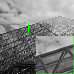
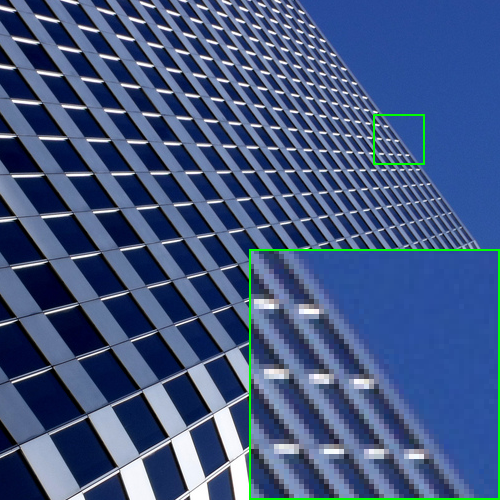
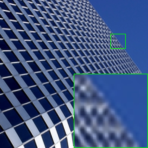
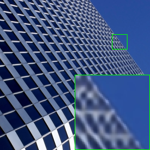
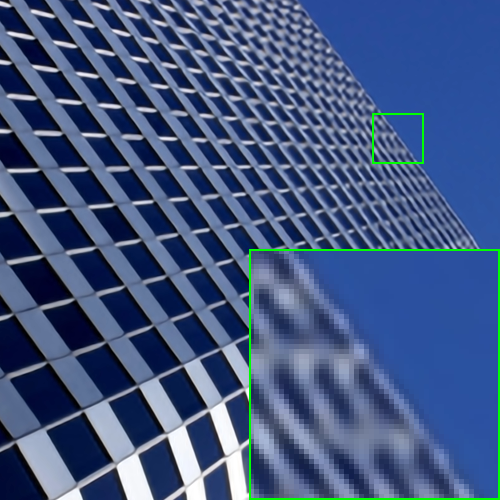
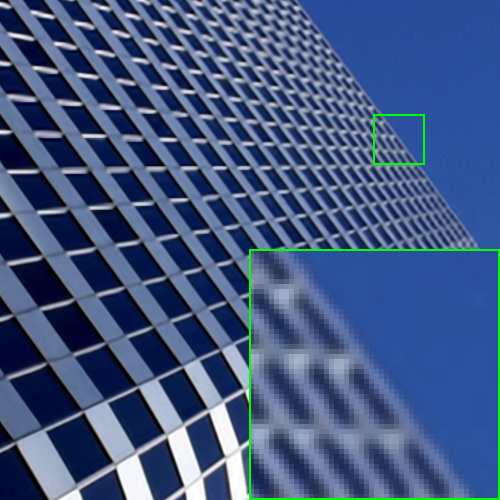
With augmentation, $600,000$ pairs of LR/HR image patches were extracted from the pair of LR/HR training images. The LR patch is of size $40\times 40$ and the HR patch is sized by $40s\times 40s$; we have trained a separate network for each scaling factor $s$($s=2,3,4$). The commonly used datasets, including Set5, Set14, the BSD100, and the Urban 100 dataset [13] containing 100 high-quality images were used in our experiments. We have compared the proposed method against several leading deep learning based image SR methods including SRCNN [34], VDSR [13] and DRCN[35], and denoising-based SR methods (i.e. TNRD[32]). For fair comparisons, the results ofall benchamrk methods are either directly cited from their papers or generated by the codes released by the authors. The PSNR results of these competing methods for the bicubic case are shown in Tables IV-V, from which one can see that the proposed method outperforms other competing methods. Portions of reconstructed HR images by different methods are shown in Figs. 10 and 11. It can be seen that the proposed method can more faithfully restore fine text details, while other methods including VDSR [13] fail to deliver the same.

TABLE IV: Results of proposed super-resolution method in Set5

Images	Scale	TNRD[32]	SRCNN[34]	VDSR[36]	DRCN[35]	Ours
Baby	2	38.53	38.54	38.75	38.80	38.83
Bird		41.31	40.91	42.42	42.68	42.70
Butterfly		33.17	32.75	34.49	34.56	34.72
Head		35.75	35.72	35.93	35.95	35.96
Woman		35.50	35.37	36.05	36.15	36.33
7
Average		36.85	36.66	37.53	37.63	37.71
Baby	3	35.28	35.25	35.38	35.50	35.56
Bird		36.09	35.48	36.66	37.05	37.20
Butterfly		28.92	27.95	29.96	30.03	30.23
Head		33.75	33.71	33.96	34.00	34.01
Woman		31.79	31.37	32.36	32.53	32.63
7
Average		33.17	32.75	33.66	33.82	33.93
Baby	4	31.30	33.13	33.41	33.51	33.61
Bird		32.99	32.52	33.54	33.78	33.93
Butterfly		26.22	25.46	27.28	27.47	27.56
Head		32.51	32.44	32.70	32.82	32.82
Woman		29.20	28.89	29.81	30.09	30.20
7
Average		30.85	30.48	31.35	31.53	31.62

TABLE V: Results of proposed super-resolution method in Set14, BSD100 and Urban100

Dataset	Scale	TNRD[32]		SRCNN[34]		VDSR[36]		DRCN[35]		Ours
		PSNR	SSIM	PSNR	SSIM	PSNR	SSIM	PSNR	SSIM	PSNR	SSIM
Set14	2	32.54	0.907	32.42	0.906	33.03	0.912	33.04	0.912	33.20	0.914
	3	29.46	0.823	29.28	0.821	29.77	0.831	29.76	0.831	29.96	0.835
	4	27.68	0.756	27.49	0.750	28.01	0.767	28.02	0.767	28.15	0.770
BSD100	2	31.40	0.888	31.36	0.888	31.90	0.896	31.85	0.894	31.94	0.896
	3	28.50	0.788	28.41	0.786	28.80	0.796	28.80	0.795	28.88	0.799
	4	27.00	0.714	26.90	0.710	27.23	0.723	27.08	0.709	27.33	0.726
Urban100	2	29.70	0.899	29.50	0.895	30.76	0.914	30.75	0.913	30.97	0.915
	3	26.44	0.807	26.24	0.799	27.15	0.828	27.08	0.824	27.33	0.831
	4	24.62	0.729	24.52	0.722	25.14	0.751	24.94	0.735	25.33	0.756

VI Conclusion

In this paper, we propose a structured analysis sparse coding (SASC) based network for image restoration and show that the structured sparse prior learned from both large-scale training dataset and the input degraded image can significantly improve the sparsity-based performance. Furthermore, we propose a network implementation of the SASC for image restoration for efficiency and better performance. Experimental results show that the proposed method performs comparably to and often even better than the current state-of-the-art restoration methods.

Figure 10: SR results of scaling factor of 3. (a) Parts of the original images of “ppt3” in Set14; (b) NCSR[7](PSNR=25.66dB); (c) SRCNN[34](PSNR=27.04dB); (d) VDSR[36](PSNR=27.86dB);(e) DRCN[35](PSNR=27.73dB); (f) Proposed method(PSNR=28.16dB)

Figure 11: SR results of scaling factor of 4. (a) Parts of the original images of “img005” in Urban100 dataset; (b) NCSR[7](PSNR=26.44dB); (c) SRCNN[34](PSNR=25.50dB); (d) VDSR[36](PSNR=26.70dB);(e) DRCN[35](PSNR=26.82dB); (f) Proposed method(PSNR=27.01dB)

References

- [1] G. Yu, G. Sapiro, and S. Mallat, “Image modeling and enhancement via structured sparse model selection,” in Image Processing (ICIP), 2010 17th IEEE International Conference on. IEEE, 2010, pp. 1641–1644.
- [2] A. Marquina and S. J. Osher, “Image super-resolution by tv-regularization and bregman iteration,” Journal of Scientific Computing, vol. 37, no. 3, pp. 367–382, 2008.
- [3] J. Yang, J. Wright, T. S. Huang, and Y. Ma, “Image super-resolution via sparse representation,” Image Processing, IEEE Transactions on, vol. 19, no. 11, pp. 2861–2873, 2010.
- [4] G. Yu, G. Sapiro, and S. Mallat, “Solving inverse problems with piecewise linear estimators: From gaussian mixture models to structured sparsity,” IEEE Transactions on Image Processing, vol. 21, no. 5, pp. 2481–2499, 2012.
- [5] W. Dong, L. Zhang, G. Shi, and X. Wu, “Image deblurring and super-resolution by adaptive sparse domain selection and adaptive regularization,” IEEE Transactions on Image Processing, vol. 20, no. 7, pp. 1838–1857, 2011.
- [6] W. Dong, L. Zhang, and G. Shi, “Centralized sparse representation for image restoration,” in Computer Vision (ICCV), 2011 IEEE International Conference on. IEEE, 2011, pp. 1259–1266.
- [7] W. Dong, L. Zhang, G. Shi, and X. Li, “Nonlocally centralized sparse representation for image restoration.” IEEE Transactions on Image Processing, vol. 22, no. 4, pp. 1620–1630, 2013.
- [8] R. Timofte, V. De Smet, and L. Van Gool, “A+: Adjusted anchored neighborhood regression for fast super-resolution,” in Asian Conference on Computer Vision. Springer, 2014, pp. 111–126.
- [9] R. Timofte, R. Rothe, and L. Van Gool, “Seven ways to improve example-based single image super resolution,” in Proceedings of the IEEE Conference on Computer Vision and Pattern Recognition, 2016, pp. 1865–1873.
- [10] C. Dong, C. C. Loy, K. He, and X. Tang, “Image super-resolution using deep convolutional networks,” IEEE transactions on pattern analysis and machine intelligence, vol. 38, no. 2, pp. 295–307, 2016.
- [11] C. Osendorfer, H. Soyer, and P. Van Der Smagt, “Image super-resolution with fast approximate convolutional sparse coding,” in International Conference on Neural Information Processing. Springer, 2014, pp. 250–257.
- [12] Z. Wang, D. Liu, J. Yang, W. Han, and T. Huang, “Deep networks for image super-resolution with sparse prior,” in Proceedings of the IEEE International Conference on Computer Vision, 2015, pp. 370–378.
- [13] J. Kim, J. Kwon Lee, and K. Mu Lee, “Accurate image super-resolution using very deep convolutional networks,” in Proceedings of the IEEE Conference on Computer Vision and Pattern Recognition, 2016, pp. 1646–1654.
- [14] ——, “Deeply-recursive convolutional network for image super-resolution,” in Proceedings of the IEEE Conference on Computer Vision and Pattern Recognition, 2016, pp. 1637–1645.
- [15] K. Egiazarian and V. Katkovnik, “Single image super-resolution via bm3d sparse coding,” in Signal Processing Conference (EUSIPCO), 2015 23rd European. IEEE, 2015, pp. 2849–2853.
- [16] S. Mallat, A wavelet tour of signal processing. Academic press, 1999.
- [17] J. Mairal, F. Bach, J. Ponce, and G. Sapiro, “Online dictionary learning for sparse coding,” in Proceedings of the 26th annual international conference on machine learning. ACM, 2009, pp. 689–696.
- [18] K. Dabov, A. Foi, V. Katkovnik, and K. Egiazarian, “Image denoising by sparse 3-d transform-domain collaborative filtering,” IEEE Transactions on image processing, vol. 16, no. 8, pp. 2080–2095, 2007.
- [19] J. Mairal, F. Bach, J. Ponce, G. Sapiro, and A. Zisserman, “Non-local sparse models for image restoration,” in Computer Vision, 2009 IEEE 12th International Conference on. IEEE, 2009, pp. 2272–2279.
- [20] J. Portilla, V. Strela, M. J. Wainwright, and E. P. Simoncelli, “Image denoising using scale mixtures of gaussians in the wavelet domain,” IEEE Transactions on Image processing, vol. 12, no. 11, pp. 1338–1351, 2003.
- [21] W. Dong, G. Shi, Y. Ma, and X. Li, “Image restoration via simultaneous sparse coding: Where structured sparsity meets gaussian scale mixture,” International Journal of Computer Vision, vol. 114, no. 2-3, pp. 217–232, 2015.
- [22] C. Dong, C. C. Loy, and X. Tang, “Accelerating the super-resolution convolutional neural network,” in European Conference on Computer Vision. Springer, 2016, pp. 391–407.
- [23] W. Shi, J. Caballero, F. Huszár, J. Totz, A. P. Aitken, R. Bishop, D. Rueckert, and Z. Wang, “Real-time single image and video super-resolution using an efficient sub-pixel convolutional neural network,” in Proceedings of the IEEE Conference on Computer Vision and Pattern Recognition, 2016, pp. 1874–1883.
- [24] Z. Cui, H. Chang, S. Shan, B. Zhong, and X. Chen, “Deep network cascade for image super-resolution,” in European Conference on Computer Vision. Springer, 2014, pp. 49–64.
- [25] Y. Chen and T. Pock, “Trainable nonlinear reaction diffusion: A flexible framework for fast and effective image restoration,” IEEE Transactions on Pattern Analysis and Machine Intelligence, 2016.
- [26] K. Gregor and Y. LeCun, “Learning fast approximations of sparse coding,” in Proceedings of the 27th International Conference on Machine Learning (ICML-10), 2010, pp. 399–406.
- [27] S. Nam, M. E. Davies, M. Elad, and R. Gribonval, “The cosparse analysis model and algorithms,” Applied and Computational Harmonic Analysis, vol. 34, no. 1, pp. 30–56, 2013.
- [28] K. Zhang, W. Zuo, Y. Chen, D. Meng, and L. Zhang, “Beyond a gaussian denoiser: Residual learning of deep cnn for image denoising,” IEEE Transactions on image processing, vol. 26, no. 7, pp. 3142–3155, 2017.
- [29] K. Dabov, A. Foi, V. Katkovnik, and K. Egiazarian, “Image denoising by sparse 3-d transform-domain collaborative filtering,” IEEE Transactions on image processing, vol. 16, no. 8, pp. 2080–2095, 2007.
- [30] D. Zoran and Y. Weiss, “From learning models of natural image patches to whole image restoration,” in Proc. of the IEEE ICCV, 2011, pp. 479–486.
- [31] S. Gu, L. Zhang, W. Zuo, and X. Feng, “Weighted nuclear norm minimization with application to image denoising,” in Proc. of the IEEE CVPR, 2014, pp. 2862–2869.
- [32] Y. Chen and T. Pock, “Trainable nonlinear reaction diffusion: A flexible framework for fast and effective image restoration,” IEEE Transactions on Pattern Analysis and Machine Intelligence, vol. 39, no. 6, pp. 1256 C–1272, 2017.
- [33] K. Zhang, W. Zuo, S. Gu, and L. Zhang, “Learning deep cnn denoiser prior for image restoration,” in Proc. of the IEEE CVPR, 2017, pp. 2808–2817.
- [34] C. Dong, C. C. Loy, K. He, and X. Tang, “Learning a deep convolutional network for image super-resolution,” in European Conference on Computer Vision. Springer, 2014, pp. 184–199.
- [35] J. Kim, J. K. Lee, and K. M. Lee, “Deeply-recursive convolutional network for image super-resolution,” in The IEEE Conference on Computer Vision and Pattern Recognition (CVPR Oral), June 2016.
- [36] ——, “Accurate image super-resolution using very deep convolutional networks,” in IEEE Conference on Computer Vision and Pattern Recognition, 2016, pp. 1646–1654.