The tilted flashing Brownian ratchet

S. N. Ethier  and Jiyeon Lee Department of Mathematics, University of Utah, 155 S. 1400 E., Salt Lake City, UT 84112, USA. e-mail: ethier@math.utah.edu.Department of Statistics, Yeungnam University, 280 Daehak-Ro, Gyeongsan, Gyeongbuk 38541, South Korea. e-mail: leejy@yu.ac.kr.
Abstract

The flashing Brownian ratchet is a stochastic process that alternates between two regimes, a one-dimensional Brownian motion and a Brownian ratchet, the latter being a one-dimensional diffusion process that drifts towards a minimum of a periodic asymmetric sawtooth potential. The result is directed motion. In the presence of a static homogeneous force that acts in the direction opposite that of the directed motion, there is a reduction (or even a reversal) of the directed motion effect. Such a process may be called a tilted flashing Brownian ratchet. We show how one can study this process numerically, using a random walk approximation or, equivalently, using numerical solution of the Fokker–Planck equation. Stochastic simulation is another viable method.

Key words and phrases: Brownian motion with drift, tilted Brownian ratchet, random walk, Parrondo’s paradox, capital-dependent Parrondo games, stochastic simulation, Fokker–Planck equation.

1 Introduction

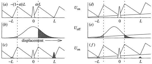
The flashing Brownian ratchet, introduced by Ajdari and Prost [1], is a stochastic process that alternates between two regimes, a one-dimensional Brownian motion and a Brownian ratchet, the latter being a one-dimensional diffusion process that drifts towards a minimum of a periodic asymmetric sawtooth potential. The result is directed motion, as shown in panels (a𝑎a)–(c𝑐c) of Figure 1 (from Harmer et al. [2]). This conceptual figure, specifically panels (a𝑎a)–(c𝑐c), although largely accurate, can be improved, as demonstrated by Ethier and Lee [4] using a random walk approximation.
Refer to caption
Figure 1: This shows how the mechanism of the ratchet potential works. The diagrams on the left, (a𝑎a)–(c𝑐c), show when there is no macroscopic gradient present and the net movement of particles is in the forward direction (defined by arrow). The diagrams on the right, (d𝑑d)–(f𝑓f), have a slight gradient present; this causes the particles to drift backwards while Uoffsubscript𝑈offU_{\text{off}} is acting. Hence the net flow of particles in the forward direction is reduced. (Figure and caption reprinted from Harmer et al. [2] with the permission of the Royal Society. A nearly identical figure appeared in Harmer and Abbott [3].)

In the presence of a static homogeneous force that acts in the direction opposite that of the directed motion, there is a reduction (or even a reversal) of the directed motion effect, as illustrated in panels (d𝑑d)–(f𝑓f) of Figure 1. (For alternative figures, see Astumian [5, Fig. 2A] and Astumian and Hänggi [6, Fig. 2].) We refer to such a process as a tilted flashing Brownian ratchet, and it is our aim here to study this process numerically, much as we did for the flashing Brownian ratchet [4], using a random walk approximation. We will see, in particular, that panels (d𝑑d)–(f𝑓f) of the conceptual Figure 1, although again largely accurate, can be improved as well.

We formulate the model using the notation of Figure 1. First, the asymmetric sawtooth potential V𝑉V can be defined by

V(x):={x/αif 0xαL,(Lx)/(1α)if αLxL,assign𝑉𝑥cases𝑥𝛼if 0xαL,𝐿𝑥1𝛼if αLxL,V(x):=\begin{cases}x/\alpha&\text{if $0\leq x\leq\alpha L$,}\\ (L-x)/(1-\alpha)&\text{if $\alpha L\leq x\leq L$,}\end{cases} (1)

extended periodically, with period L𝐿L, to all of 𝐑𝐑{\bf R}. Here 0<α<10𝛼10<\alpha<1 and L>0𝐿0L>0, and α1/2𝛼12\alpha\neq 1/2 by virtue of the asymmetry. (α𝛼\alpha is a shape parameter, and L𝐿L is the period and the amplitude of the potential.) The tilted Brownian ratchet is a one-dimensional diffusion process with diffusion coefficient 1 and drift coefficient μ𝜇\mu of the form, for some γ>0𝛾0\gamma>0 and κ𝜅\kappa real,

μ(x):=[γV(x)+κ]={γ/ακif 0x<αL,γ/(1α)κif αLx<L,assign𝜇𝑥delimited-[]𝛾superscript𝑉𝑥𝜅cases𝛾𝛼𝜅if 0x<αL,𝛾1𝛼𝜅if αLx<L,\mu(x):=-[\gamma V^{\prime}(x)+\kappa]=\begin{cases}-\gamma/\alpha-\kappa&\text{if $0\leq x<\alpha L$,}\\ \gamma/(1-\alpha)-\kappa&\text{if $\alpha L\leq x<L$,}\end{cases} (2)

again extended periodically, with period L𝐿L, to all of 𝐑𝐑{\bf R}. Such a process Xtsubscript𝑋𝑡X_{t} is governed by the Itô stochastic differential equation (SDE)

dXt=[γV(Xt)+κ]dt+dBt,𝑑subscript𝑋𝑡delimited-[]𝛾superscript𝑉subscript𝑋𝑡𝜅𝑑𝑡𝑑subscript𝐵𝑡dX_{t}=-[\gamma V^{\prime}(X_{t})+\kappa]\,dt+dB_{t}, (3)

where Btsubscript𝐵𝑡B_{t} is standard Brownian motion. This diffusion process drifts to the left on (nL,nL+αL)𝑛𝐿𝑛𝐿𝛼𝐿(nL,nL+\alpha L) and drifts to the right on (nL(1α)L,nL)𝑛𝐿1𝛼𝐿𝑛𝐿(nL-(1-\alpha)L,nL), for each n𝐙𝑛𝐙n\in{\bf Z}, provided γ/α<κ<γ/(1α)𝛾𝛼𝜅𝛾1𝛼-\gamma/\alpha<\kappa<\gamma/(1-\alpha). In other words, it drifts towards a minimum of the sawtooth potential γV𝛾𝑉\gamma V (or a local minimum of the tilted sawtooth potential γV(x)+κx𝛾𝑉𝑥𝜅𝑥\gamma V(x)+\kappa x). γL𝛾𝐿\gamma L is the amplitude of the potential and κ𝜅\kappa is the slope of the tilt.

While the inequalities γ/α<κ<γ/(1α)𝛾𝛼𝜅𝛾1𝛼-\gamma/\alpha<\kappa<\gamma/(1-\alpha) are not needed to define the process, they are needed for the tilted ratchet to remain a ratchet. Furthermore, we usually assume that the static homogeneous force acts in the direction opposite that of the directed motion, that is, (12α)κ>012𝛼𝜅0\big{(}\frac{1}{2}-\alpha\big{)}\kappa>0, but this is not essential either.

It may be helpful to reconcile our model with those in the literature. Our tilted Brownian ratchet is equivalent to what Reimann [7, Eq. (2.34)] called a “tilted Smoluchowski–Feynman ratchet,” acknowledging two of the pioneers of the subject. It is given by the Langevin equation

ηx˙(t)=βV(x(t))+F+2ηkBTξ(t),𝜂˙𝑥𝑡𝛽superscript𝑉𝑥𝑡𝐹2𝜂subscript𝑘B𝑇𝜉𝑡\eta\,\dot{x}(t)=-\beta V^{\prime}(x(t))+F+\sqrt{2\eta k_{\text{B}}T}\,\xi(t), (4)

where x(t)𝑥𝑡x(t) is the position of the particle at time t𝑡t, V𝑉V is the periodic sawtooth potential (1), βL𝛽𝐿\beta L is the amplitude of the potential (β𝛽\beta does not appear in [7] because its V𝑉V is our βV𝛽𝑉\beta V), F𝐹F is an additional static homogeneous force, ξ(t)𝜉𝑡\xi(t) is a Gaussian white noise with mean ξ(t)=0delimited-⟨⟩𝜉𝑡0\langle\xi(t)\rangle=0 and covariance ξ(t)ξ(s)=δ(ts)delimited-⟨⟩𝜉𝑡𝜉𝑠𝛿𝑡𝑠\langle\xi(t)\xi(s)\rangle=\delta(t-s), η𝜂\eta is a friction coefficient, kBsubscript𝑘Bk_{\text{B}} is Boltzmann’s constant, and T𝑇T is temperature. We interpret this equation mathematically as the SDE

ηdx(t)=[βV(x(t))+F]dt+2ηkBTdb(t),𝜂𝑑𝑥𝑡delimited-[]𝛽superscript𝑉𝑥𝑡𝐹𝑑𝑡2𝜂subscript𝑘B𝑇𝑑𝑏𝑡\eta\,dx(t)=[-\beta V^{\prime}(x(t))+F]\,dt+\sqrt{2\eta k_{\text{B}}T}\,db(t),

where b(t)𝑏𝑡b(t) is standard Brownian motion, or

dx(t)=η1[βV(x(t))+F]dt+σdb(t)𝑑𝑥𝑡superscript𝜂1delimited-[]𝛽superscript𝑉𝑥𝑡𝐹𝑑𝑡𝜎𝑑𝑏𝑡dx(t)=\eta^{-1}[-\beta V^{\prime}(x(t))+F]\,dt+\sigma\,db(t) (5)

with σ=2η1kBT𝜎2superscript𝜂1subscript𝑘B𝑇\sigma=\sqrt{2\eta^{-1}k_{\text{B}}T}. With the time change Xt:=x(σ2t)assignsubscript𝑋𝑡𝑥superscript𝜎2𝑡X_{t}:=x(\sigma^{-2}t) and standard Brownian motion Bt:=σb(σ2t)assignsubscript𝐵𝑡𝜎𝑏superscript𝜎2𝑡B_{t}:=\sigma\,b(\sigma^{-2}t), (5) becomes

dXt=σ2η1[βV(Xt)+F]dt+dBt,𝑑subscript𝑋𝑡superscript𝜎2superscript𝜂1delimited-[]𝛽superscript𝑉subscript𝑋𝑡𝐹𝑑𝑡𝑑subscript𝐵𝑡dX_{t}=\sigma^{-2}\eta^{-1}[-\beta V^{\prime}(X_{t})+F]\,dt+dB_{t},

which is (3) with

γ=σ2η1β=β2kBTandκ=σ2η1F=F2kBT.formulae-sequence𝛾superscript𝜎2superscript𝜂1𝛽𝛽2subscript𝑘B𝑇and𝜅superscript𝜎2superscript𝜂1𝐹𝐹2subscript𝑘B𝑇\gamma=\sigma^{-2}\eta^{-1}\beta=\frac{\beta}{2k_{\text{B}}T}\quad\text{and}\quad\kappa=-\sigma^{-2}\eta^{-1}F=-\frac{F}{2k_{\text{B}}T}.

Other sources with equations similar to (4) include Reimann and Hänggi [8, Eq. (11)], Parrondo and de Cisneros [9, Eq. (22)], Dinis [10, Eq. (1.88) with α(t)=1𝛼𝑡1\alpha(t)=1], and Hänggi and Marchesoni [11, Eq. (3)].

Given time parameters τ1,τ2>0subscript𝜏1subscript𝜏20\tau_{1},\tau_{2}>0, the tilted flashing Brownian ratchet is a time-inhomogeneous one-dimensional diffusion process that evolves as a Brownian motion with drift κ𝜅-\kappa (i.e., Btκtsubscript𝐵𝑡𝜅𝑡B_{t}-\kappa t) on [0,τ1]0subscript𝜏1[0,\tau_{1}] (potential “off”), then as the tilted Brownian ratchet (3) on [τ1,τ1+τ2]subscript𝜏1subscript𝜏1subscript𝜏2[\tau_{1},\tau_{1}+\tau_{2}] (potential “on”), and so on, alternating between these two regimes. Such a process Ytsubscript𝑌𝑡Y_{t} is governed by the SDE

dYt=[γζ(t)V(Yt)+κ]dt+dBt,𝑑subscript𝑌𝑡delimited-[]𝛾𝜁𝑡superscript𝑉subscript𝑌𝑡𝜅𝑑𝑡𝑑subscript𝐵𝑡dY_{t}=-[\gamma\zeta(t)V^{\prime}(Y_{t})+\kappa]\,dt+dB_{t}, (6)

where111The quantity mod(t,τ)mod𝑡𝜏\text{mod}(t,\tau) is defined as the remainder (in [0,τ)0𝜏[0,\tau)) when t𝑡t is divided by τ𝜏\tau.

ζ(t):={0if mod(t,τ1+τ2)<τ1,1if mod(t,τ1+τ2)τ1.assign𝜁𝑡cases0if mod(t,τ1+τ2)<τ1,1if mod(t,τ1+τ2)τ1.\zeta(t):=\begin{cases}0&\text{if mod$(t,\tau_{1}+\tau_{2})<\tau_{1}$,}\\ 1&\text{if mod$(t,\tau_{1}+\tau_{2})\geq\tau_{1}$.}\end{cases} (7)

The flashing Brownian ratchet is the process that motivated Parrondo’s paradox (Harmer and Abbott [3, 12]), in which two fair games of chance, when alternated in some way, produce a winning (or losing) game. The tilted flashing Brownian ratchet, which is a flashing Brownian ratchet in the presence of a static homogeneous force, can be discretized to yield a stronger form of Parrondo’s paradox, in which two losing games combine to win (or two winning games combine to lose). In Section 2 we provide a general formulation of Parrondo’s paradox motivated by the tilted flashing Brownian ratchet. These capital-dependent Parrondo games are modified in Section 3 so as to yield our random walk approximation, which we then suggest can be improved. Other ways of numerically studying the tilted flashing Brownian ratchet include stochastic simulation using the Euler–Maruyama method (Section 4), and numerical solution of the Fokker–Planck equation using the finite-difference method (Section 5). We show in Sections 6 and 7 that the conceptual Figure 1 is not an entirely accurate representation of the behavior of the tilted flashing Brownian ratchet. This conclusion can be deduced from the random walk approximation, from stochastic simulation, or from numerical solution of the Fokker–Planck equation.

2 Parrondo games and tilted Brownian ratchets

Parrondo’s paradox is a discretization and reinterpretation of the flashing Brownian ratchet, as explained in [4] and in various other references [2, 3, 12, 14, 13, 15, 16, 17]. The role of displacement is played by profit in a game of chance. The role of Brownian motion is played by game A𝐴A, whose cumulative-profit process is a simple symmetric random walk on Z. The role of the Brownian ratchet is played by game B𝐵B, whose cumulative-profit process is a simple random walk on Z with periodic state-dependent transition probabilities. The role of the flashing Brownian ratchet is played by some combination of games A𝐴A and B𝐵B, either a random mixture (i.e., cA+(1c)B𝑐𝐴1𝑐𝐵cA+(1-c)B, where 0<c<10𝑐10<c<1) or a nonrandom periodic pattern (e.g., AABBAABB𝐴𝐴𝐵𝐵𝐴𝐴𝐵𝐵AABB\,AABB\,\cdots). Finally, the role of tilt is played by a bias parameter in the transition probabilities of the random walks.

Let 0<α<10𝛼10<\alpha<1 and assume that α𝛼\alpha is rational, so that α=l/L𝛼𝑙𝐿\alpha=l/L for some relatively prime positive integers 1l<L1𝑙𝐿1\leq l<L. The cumulative-profit process of game B𝐵B is the simple random walk on Z with periodic state-dependent transition probabilities of the form

P(j,j+1):={p0if mod(j,L)<l,p1if mod(j,L)l,assign𝑃𝑗𝑗1casessubscript𝑝0if mod(j,L)<l,subscript𝑝1if mod(j,L)l,P(j,j+1):=\begin{cases}p_{0}&\text{if mod$(j,L)<l$,}\\ p_{1}&\text{if mod$(j,L)\geq l$,}\end{cases} (8)

and P(j,j1)=1P(j,j+1)𝑃𝑗𝑗11𝑃𝑗𝑗1P(j,j-1)=1-P(j,j+1), where 0<p0<1/2<p1<10subscript𝑝012subscript𝑝110<p_{0}<1/2<p_{1}<1. Because of the period-L𝐿L transition probabilities, the unique reversible invariant measure π𝜋\pi must have period L𝐿L (i.e., π(j)=π(j+L)𝜋𝑗𝜋𝑗𝐿\pi(j)=\pi(j+L)) for the random walk to be recurrent. We can confirm that the detailed balance conditions have a solution if and only if (1p0)l(1p1)Ll=p0lp1Llsuperscript1subscript𝑝0𝑙superscript1subscript𝑝1𝐿𝑙superscriptsubscript𝑝0𝑙superscriptsubscript𝑝1𝐿𝑙(1-p_{0})^{l}(1-p_{1})^{L-l}=p_{0}^{l}p_{1}^{L-l}. Solving for p1subscript𝑝1p_{1}, we obtain

p1=11+[p0/(1p0)]α/(1α).subscript𝑝111superscriptdelimited-[]subscript𝑝01subscript𝑝0𝛼1𝛼p_{1}=\frac{1}{1+[p_{0}/(1-p_{0})]^{\alpha/(1-\alpha)}}.

With the α/(1α)𝛼1𝛼\alpha/(1-\alpha)th power in the denominator denoted by ρ𝜌\rho, the requirements that 0<p0<1/2<p1<10subscript𝑝012subscript𝑝110<p_{0}<1/2<p_{1}<1 become 0<ρ<10𝜌10<\rho<1, and

p0=ρ(1α)/α1+ρ(1α)/αandp1=11+ρ.formulae-sequencesubscript𝑝0superscript𝜌1𝛼𝛼1superscript𝜌1𝛼𝛼andsubscript𝑝111𝜌p_{0}=\frac{\rho^{(1-\alpha)/\alpha}}{1+\rho^{(1-\alpha)/\alpha}}\quad\text{and}\quad p_{1}=\frac{1}{1+\rho}. (9)

As shown in [4], game B𝐵B is fair (asymptotically), whereas the random mixture cA+(1c)B𝑐𝐴1𝑐𝐵cA+(1-c)B, where 0<c<10𝑐10<c<1, is winning if α<1/2𝛼12\alpha<1/2 and losing if α>1/2𝛼12\alpha>1/2. Thus, two fair games combine to win if α<1/2𝛼12\alpha<1/2, which is the Parrondo effect, and combine to lose if α>1/2𝛼12\alpha>1/2, which is the anti-Parrondo effect. Both are examples of Parrondo’s paradox. Analysis of nonrandom periodic patterns is more complicated.

A slightly stronger form of the Parrondo effect occurs when two losing games combine to win. That can be achieved by replacing the cumulative-profit process of game A𝐴A by the simple random walk on Z with

P(j,j+1)=p:=12ε𝑃𝑗𝑗1𝑝assign12𝜀P(j,j+1)=p:=\frac{1}{2}-\varepsilon (10)

and P(j,j1)=1P(j,j+1)𝑃𝑗𝑗11𝑃𝑗𝑗1P(j,j-1)=1-P(j,j+1), where the bias parameter ε>0𝜀0\varepsilon>0 is sufficiently small, and replacing the cumulative-profit process of game B𝐵B by the simple random walk on Z with periodic state-dependent transition probabilities of the form (8) with α<1/2𝛼12\alpha<1/2 but with (9) replaced by

p0=ρ(1α)/α1+ρ(1α)/αεandp1=11+ρε.formulae-sequencesubscript𝑝0superscript𝜌1𝛼𝛼1superscript𝜌1𝛼𝛼𝜀andsubscript𝑝111𝜌𝜀p_{0}=\frac{\rho^{(1-\alpha)/\alpha}}{1+\rho^{(1-\alpha)/\alpha}}-\varepsilon\quad\text{and}\quad p_{1}=\frac{1}{1+\rho}-\varepsilon. (11)

Parrondo’s original formulation of the games assumed α=1/3𝛼13\alpha=1/3, L=3𝐿3L=3, ρ=1/3𝜌13\rho=1/3, and ε=1/200𝜀1200\varepsilon=1/200.

A slightly stronger form of the anti-Parrondo effect occurs when two winning games combine to lose. That can be achieved as in the preceding paragraph but with α>1/2𝛼12\alpha>1/2 and ε<0𝜀0\varepsilon<0, where |ε|𝜀|\varepsilon| is sufficiently small.

3 Random walk approximation

We have seen that a discretization of the tilted flashing Brownian ratchet yields capital-dependent Parrondo games with a bias parameter. In this section we demonstrate the converse: A continuization of capital-dependent Parrondo games with a bias parameter yields the tilted flashing Brownian ratchet.

Let 0<α<10𝛼10<\alpha<1 and assume that α𝛼\alpha is rational, so that α=l/L𝛼𝑙𝐿\alpha=l/L for some relatively prime positive integers 1l<L1𝑙𝐿1\leq l<L. Consider a sequence of simple random walks on 𝐙𝐙{\bf Z} with periodic state-dependent transition probabilities defined as follows. For each n1𝑛1n\geq 1, we let

Pn(j,j+1):={p0if mod(j,nL)<nl,p1if mod(j,nL)nl,assignsubscript𝑃𝑛𝑗𝑗1casessubscript𝑝0if mod(j,nL)<nl,subscript𝑝1if mod(j,nL)nl,P_{n}(j,j+1):=\begin{cases}p_{0}&\text{if mod$(j,nL)<nl$,}\\ p_{1}&\text{if mod$(j,nL)\geq nl$,}\end{cases} (12)

and Pn(j,j1)=1Pn(j,j+1)subscript𝑃𝑛𝑗𝑗11subscript𝑃𝑛𝑗𝑗1P_{n}(j,j-1)=1-P_{n}(j,j+1), where p0subscript𝑝0p_{0} and p1subscript𝑝1p_{1} are as in (11). The special case of (12) in which n=1𝑛1n=1 is precisely (8).

We will let n𝑛n\to\infty but first we require

ρ=1λnandε=κ2n,formulae-sequence𝜌1𝜆𝑛and𝜀𝜅2𝑛\rho=1-\frac{\lambda}{n}\quad\text{and}\quad\varepsilon=\frac{\kappa}{2n}, (13)

where λ>0𝜆0\lambda>0 and κ𝜅\kappa is real, then we rescale time by allowing n2superscript𝑛2n^{2} jumps per unit of time, and finally we rescale space by dividing by n𝑛n. The result in the limit as n𝑛n\to\infty is a tilted Brownian ratchet.

We denote by D𝐑[0,)subscript𝐷𝐑0D_{\bf R}[0,\infty) the space of real-valued functions on [0,)0[0,\infty) that are right-continuous with left limits, and we give it the Skorokhod topology.

Theorem 1 (Random walk approximation of tilted Brownian ratchet).

Let λ>0𝜆0\lambda>0 and κ𝜅\kappa be real. For n=1,2,𝑛12n=1,2,\ldots (((and n𝑛n sufficiently large that ρ,p0,p1(0,1))\rho,p_{0},p_{1}\in(0,1)), let {Xn(k),k=0,1,}formulae-sequencesubscript𝑋𝑛𝑘𝑘01\{X_{n}(k),\,k=0,1,\ldots\} denote the random walk on 𝐙𝐙{\bf Z} defined by (11)–(13), and let {Xt,t0}subscript𝑋𝑡𝑡0\{X_{t},\,t\geq 0\} denote the tilted Brownian ratchet with parameters γ:=λ(1α)/2assign𝛾𝜆1𝛼2\gamma:=\lambda(1-\alpha)/2 and κ𝜅\kappa. If Xn(0)/nsubscript𝑋𝑛0𝑛X_{n}(0)/n converges in distribution to X0subscript𝑋0X_{0} as n𝑛n\to\infty, then {Xn(n2t)/n,t0}subscript𝑋𝑛superscript𝑛2𝑡𝑛𝑡0\{X_{n}(\lfloor n^{2}t\rfloor)/n,\,t\geq 0\} converges in distribution in D𝐑[0,)subscript𝐷𝐑0D_{\bf R}[0,\infty) to {Xt,t0}subscript𝑋𝑡𝑡0\{X_{t},\,t\geq 0\} as n𝑛n\to\infty.

Proof.

The argument is essentially as in the proof of Theorem 1 of [4], except that, if μnμsubscript𝜇𝑛𝜇\mu_{n}\to\mu as n𝑛n\to\infty, then

12(1+μnn)=p0121subscript𝜇𝑛𝑛subscript𝑝0\displaystyle\frac{1}{2}\bigg{(}1+\frac{\mu_{n}}{n}\bigg{)}=p_{0} =(1λ/n)(1α)/α1+(1λ/n)(1α)/ακ2nabsentsuperscript1𝜆𝑛1𝛼𝛼1superscript1𝜆𝑛1𝛼𝛼𝜅2𝑛\displaystyle=\frac{(1-\lambda/n)^{(1-\alpha)/\alpha}}{1+(1-\lambda/n)^{(1-\alpha)/\alpha}}-\frac{\kappa}{2n}
=12(1λ(1α)2nακn+o(n1))absent121𝜆1𝛼2𝑛𝛼𝜅𝑛𝑜superscript𝑛1\displaystyle=\frac{1}{2}\bigg{(}1-\frac{\lambda(1-\alpha)}{2n\alpha}-\frac{\kappa}{n}+o(n^{-1})\bigg{)}

leads to μ=λ(1α)/(2α)κ=γ/ακ𝜇𝜆1𝛼2𝛼𝜅𝛾𝛼𝜅\mu=-\lambda(1-\alpha)/(2\alpha)-\kappa=-\gamma/\alpha-\kappa, and

12(1+μnn)=p1121subscript𝜇𝑛𝑛subscript𝑝1\displaystyle\frac{1}{2}\bigg{(}1+\frac{\mu_{n}}{n}\bigg{)}=p_{1} =11+(1λ/n)κ2nabsent111𝜆𝑛𝜅2𝑛\displaystyle=\frac{1}{1+(1-\lambda/n)}-\frac{\kappa}{2n}
=12(1+λ2nκn+o(n1))absent121𝜆2𝑛𝜅𝑛𝑜superscript𝑛1\displaystyle=\frac{1}{2}\bigg{(}1+\frac{\lambda}{2n}-\frac{\kappa}{n}+o(n^{-1})\bigg{)}

leads to μ=λ/2κ=γ/(1α)κ𝜇𝜆2𝜅𝛾1𝛼𝜅\mu=\lambda/2-\kappa=\gamma/(1-\alpha)-\kappa. ∎

Ordinarily, a Markov chain is given, and one attempts to approximate it by a diffusion process that is more amenable to analysis. There are many examples in such areas as population genetics and queueing theory. Here we are doing the opposite. A diffusion process is given, and we want to approximate it by a random walk that is more amenable to computation. The sequence of random walks in Theorem 1 has a clear relationship to the capital-dependent Parrondo games of Section 2, but it is not written in stone. Perhaps it can be improved, in the sense of converging faster, thereby yielding a better approximation. Towards this end we find a clue in the proof of Theorem 1. We replace (11) and (13) by

p0=12(1λ(1α)2nακn)andp1=12(1+λ2nκn).formulae-sequencesubscript𝑝0121𝜆1𝛼2𝑛𝛼𝜅𝑛andsubscript𝑝1121𝜆2𝑛𝜅𝑛p_{0}=\frac{1}{2}\bigg{(}1-\frac{\lambda(1-\alpha)}{2n\alpha}-\frac{\kappa}{n}\bigg{)}\quad\text{and}\quad p_{1}=\frac{1}{2}\bigg{(}1+\frac{\lambda}{2n}-\frac{\kappa}{n}\bigg{)}. (14)
Theorem 1 (Improved random walk approximation of tilted Brownian ratchet).

Theorem 1 remains true with “(11)–(13)” replaced by “(12) and (14)”.

For the next theorem, we assume that the time parameters τ1,τ2>0subscript𝜏1subscript𝜏20\tau_{1},\tau_{2}>0 of the tilted flashing Brownian ratchet are rational. We let m𝑚m be the smallest positive integer such that m2τ1superscript𝑚2subscript𝜏1m^{2}\tau_{1} and m2τ2superscript𝑚2subscript𝜏2m^{2}\tau_{2} are integers. Recall (10) and augment it with (13).

Theorem 2 (Random walk approximation of tilted flashing Brownian ratchet).

Let λ>0𝜆0\lambda>0, κ𝜅\kappa be real, and τ1subscript𝜏1\tau_{1}, τ2subscript𝜏2\tau_{2}, and m𝑚m be as above. For n=m,2m,3m,𝑛𝑚2𝑚3𝑚n=m,2m,3m,\ldots (((and n𝑛n sufficiently large that p,ρ,p0,p1(0,1))p,\rho,p_{0},p_{1}\in(0,1)), let {Yn(k),k=0,1,}formulae-sequencesubscript𝑌𝑛𝑘𝑘01\{Y_{n}(k),\,k=0,1,\ldots\} denote the time-inhomogeneous random walk on 𝐙𝐙{\bf Z} that evolves as the simple random walk with Pn0(j,j+1)=p=1Pn0(j,j1)superscriptsubscript𝑃𝑛0𝑗𝑗1𝑝1superscriptsubscript𝑃𝑛0𝑗𝑗1P_{n}^{0}(j,j+1)=p=1-P_{n}^{0}(j,j-1) for n2τ1superscript𝑛2subscript𝜏1n^{2}\tau_{1} steps, then as the random walk of Theorem 1 for n2τ2superscript𝑛2subscript𝜏2n^{2}\tau_{2} steps, and so on, alternating in this way. Let {Yt,t0}subscript𝑌𝑡𝑡0\{Y_{t},\,t\geq 0\} denote the tilted flashing Brownian ratchet with parameters γ:=λ(1α)/2assign𝛾𝜆1𝛼2\gamma:=\lambda(1-\alpha)/2, κ𝜅\kappa, τ1subscript𝜏1\tau_{1}, and τ2subscript𝜏2\tau_{2}. If Yn(0)/nsubscript𝑌𝑛0𝑛Y_{n}(0)/n converges in distribution to Y0subscript𝑌0Y_{0} as n𝑛n\to\infty, then {Yn(n2t)/n,t0}subscript𝑌𝑛superscript𝑛2𝑡𝑛𝑡0\{Y_{n}(\lfloor n^{2}t\rfloor)/n,\,t\geq 0\} converges in distribution in D𝐑[0,)subscript𝐷𝐑0D_{\bf R}[0,\infty) to {Yt,t0}subscript𝑌𝑡𝑡0\{Y_{t},\,t\geq 0\} as n𝑛n\to\infty. (((Here n𝑛n\to\infty through multiples of m𝑚m.)))

Proof.

The argument is essentially as in the proof of Theorem 2 of [4]. ∎

Theorem 2 (Improved random walk approximation of tilted flashing Brownian ratchet).

Theorem 2 remains true with “Theorem 1” replaced by “Theorem 1”.

It seems clear, and computations suggest, that the random walk approximation of Theorem 2 is more accurate than that of Theorem 2, thereby justifying the use of the adjective “improved”.

4 Simulation of the solution of the SDE

Here we approximate the solution of the SDE (3) by the solution of the stochastic difference equation (with time step hh)

X((k+1)h)X(kh)𝑋𝑘1𝑋𝑘\displaystyle X((k+1)h)-X(kh)
=[γV(X(kh))+κ]h+B((k+1)h)B(kh),k=0,1,,formulae-sequenceabsentdelimited-[]𝛾superscript𝑉𝑋𝑘𝜅𝐵𝑘1𝐵𝑘𝑘01\displaystyle\qquad{}=-[\gamma V^{\prime}(X(kh))+\kappa]h+B((k+1)h)-B(kh),\quad k=0,1,\ldots,

often called the Euler–Maruyama method. Here the Brownian increments B((k+1)h)B(kh)𝐵𝑘1𝐵𝑘B((k+1)h)-B(kh) are independent normal random variables with mean 0 and variance hh. To justify the method, we take h=1/n21superscript𝑛2h=1/n^{2} and Xn(k):=X(kh)assignsubscript𝑋𝑛𝑘𝑋𝑘X_{n}(k):=X(kh), obtaining the sequence of stochastic difference equations

Xn(k+1)Xn(k)=γV(Xn(k))+κn2+Zk+1n,k=0,1,,formulae-sequencesubscript𝑋𝑛𝑘1subscript𝑋𝑛𝑘𝛾superscript𝑉subscript𝑋𝑛𝑘𝜅superscript𝑛2subscript𝑍𝑘1𝑛𝑘01X_{n}(k+1)-X_{n}(k)=-\frac{\gamma V^{\prime}(X_{n}(k))+\kappa}{n^{2}}+\frac{Z_{k+1}}{n},\quad k=0,1,\ldots, (15)

where Z1,Z2,subscript𝑍1subscript𝑍2Z_{1},Z_{2},\ldots are independent standard normal random variables.

Theorem 3 (Simulation of the tilted Brownian ratchet).

Let γ>0𝛾0\gamma>0 and κ𝜅\kappa be real. For n=1,2,𝑛12n=1,2,\ldots, define the continuous-state Markov chain {Xn(k),k=0,1,}formulae-sequencesubscript𝑋𝑛𝑘𝑘01\{X_{n}(k),\,k=0,1,\ldots\} by (15) (((given the initial state Xn(0)subscript𝑋𝑛0X_{n}(0), independent of Z1,Z2,)Z_{1},Z_{2},\ldots), and let {Xt,t0}subscript𝑋𝑡𝑡0\{X_{t},\,t\geq 0\} denote the tilted Brownian ratchet with parameters γ𝛾\gamma and κ𝜅\kappa. If Xn(0)subscript𝑋𝑛0X_{n}(0) converges in distribution to X0subscript𝑋0X_{0} as n𝑛n\to\infty, then {Xn(n2t),t0}subscript𝑋𝑛superscript𝑛2𝑡𝑡0\{X_{n}(\lfloor n^{2}t\rfloor),\,t\geq 0\} converges in distribution in D𝐑[0,)subscript𝐷𝐑0D_{\bf R}[0,\infty) to {Xt,t0}subscript𝑋𝑡𝑡0\{X_{t},\,t\geq 0\} as n𝑛n\to\infty.

Proof.

The proof is a straightforward application of Corollary 4.8.17 of [18]. ∎

Again, we assume that the time parameters τ1,τ2>0subscript𝜏1subscript𝜏20\tau_{1},\tau_{2}>0 of the tilted flashing Brownian ratchet are rational. We let m𝑚m be the smallest positive integer such that m2τ1superscript𝑚2subscript𝜏1m^{2}\tau_{1} and m2τ2superscript𝑚2subscript𝜏2m^{2}\tau_{2} are integers.

We now modify (15) to

Yn(k+1)Yn(k)=γζ(k/n2)V(Yn(k))+κn2+Zk+1n,k=0,1,,formulae-sequencesubscript𝑌𝑛𝑘1subscript𝑌𝑛𝑘𝛾𝜁𝑘superscript𝑛2superscript𝑉subscript𝑌𝑛𝑘𝜅superscript𝑛2subscript𝑍𝑘1𝑛𝑘01Y_{n}(k+1)-Y_{n}(k)=-\frac{\gamma\zeta(k/n^{2})V^{\prime}(Y_{n}(k))+\kappa}{n^{2}}+\frac{Z_{k+1}}{n},\quad k=0,1,\ldots, (16)

where Z1,Z2,subscript𝑍1subscript𝑍2Z_{1},Z_{2},\ldots are independent standard normal random variables and ζ𝜁\zeta is the function defined in (7).

Theorem 4 (Simulation of the tilted flashing Brownian ratchet).

Let γ>0𝛾0\gamma>0, κ𝜅\kappa be real, and τ1subscript𝜏1\tau_{1}, τ2subscript𝜏2\tau_{2}, and m𝑚m be as above. For n=m,2m,3m,𝑛𝑚2𝑚3𝑚n=m,2m,3m,\ldots, define the continuous-state Markov chain {Yn(k),k=0,1,}formulae-sequencesubscript𝑌𝑛𝑘𝑘01\{Y_{n}(k),\,k=0,1,\ldots\} by (16) (((given the initial state Yn(0)subscript𝑌𝑛0Y_{n}(0), independent of Z1,Z2,)Z_{1},Z_{2},\ldots), and let {Yt,t0}subscript𝑌𝑡𝑡0\{Y_{t},\,t\geq 0\} denote the tilted flashing Brownian ratchet with parameters γ𝛾\gamma, κ𝜅\kappa, τ1subscript𝜏1\tau_{1}, and τ2subscript𝜏2\tau_{2}. If Yn(0)subscript𝑌𝑛0Y_{n}(0) converges in distribution to Y0subscript𝑌0Y_{0} as n𝑛n\to\infty, then {Yn(n2t),t0}subscript𝑌𝑛superscript𝑛2𝑡𝑡0\{Y_{n}(\lfloor n^{2}t\rfloor),\,t\geq 0\} converges in distribution in D𝐑[0,)subscript𝐷𝐑0D_{\bf R}[0,\infty) to {Yt,t0}subscript𝑌𝑡𝑡0\{Y_{t},\,t\geq 0\} as n𝑛n\to\infty. (((Here n𝑛n\to\infty through multiples of m𝑚m.)))

Suppose, for example, we want to simulate the distribution of Yτ1+τ2subscript𝑌subscript𝜏1subscript𝜏2Y_{\tau_{1}+\tau_{2}}. We choose an n𝑛n, say n=100𝑛100n=100, and simulate Yn(n2(τ1+τ2))subscript𝑌𝑛superscript𝑛2subscript𝜏1subscript𝜏2Y_{n}(n^{2}(\tau_{1}+\tau_{2})) by computing (16) for k=0,1,,n2(τ1+τ2)1𝑘01superscript𝑛2subscript𝜏1subscript𝜏21k=0,1,\ldots,n^{2}(\tau_{1}+\tau_{2})-1. Repeating this computation a large number of times (e.g., 106superscript10610^{6}) will yield a histogram that approximates the distribution of interest.

Simulations of the flashing Brownian ratchet (albeit modified slightly from the one defined here) can be found in several sources, including Kinderlehrer and Kowalczyk [19, Fig. 2] and Hänggi and Marchesoni [11, Fig. 4].

5 Numerical solution of the FP equation

The Fokker–Planck equation (or Kolmogorov forward equation) is the equation for the transition density p(t,x,y)𝑝𝑡𝑥𝑦p(t,x,y) of the diffusion process with diffusion coefficient 1 and drift coefficient μ𝜇\mu, namely

tp(t,x,y)=122y2p(t,x,y)y[μ(y)p(t,x,y)].𝑡𝑝𝑡𝑥𝑦12superscript2superscript𝑦2𝑝𝑡𝑥𝑦𝑦delimited-[]𝜇𝑦𝑝𝑡𝑥𝑦\frac{\partial}{\partial t}p(t,x,y)=\frac{1}{2}\frac{\partial^{2}}{\partial y^{2}}p(t,x,y)-\frac{\partial}{\partial y}[\mu(y)p(t,x,y)].

We can solve it numerically using the finite-difference method. We take tk:=k/n2assignsubscript𝑡𝑘𝑘superscript𝑛2t_{k}:=k/n^{2} and yj:=j/nassignsubscript𝑦𝑗𝑗𝑛y_{j}:=j/n, hence Δt:=tk+1tk=1/n2assignΔ𝑡subscript𝑡𝑘1subscript𝑡𝑘1superscript𝑛2\Delta t:=t_{k+1}-t_{k}=1/n^{2} and Δy:=yj+1yj=1/nassignΔ𝑦subscript𝑦𝑗1subscript𝑦𝑗1𝑛\Delta y:=y_{j+1}-y_{j}=1/n. We write p(t,y)𝑝𝑡𝑦p(t,y) for p(t,x,y)𝑝𝑡𝑥𝑦p(t,x,y) (the initial state x𝑥x is fixed) to get

p(tk+1,yj)p(tk,yj)Δt𝑝subscript𝑡𝑘1subscript𝑦𝑗𝑝subscript𝑡𝑘subscript𝑦𝑗Δ𝑡\displaystyle\frac{p(t_{k+1},y_{j})-p(t_{k},y_{j})}{\Delta t} =12p(tk,yj+1)2p(tk,yj)+p(tk,yj1)(Δy)2absent12𝑝subscript𝑡𝑘subscript𝑦𝑗12𝑝subscript𝑡𝑘subscript𝑦𝑗𝑝subscript𝑡𝑘subscript𝑦𝑗1superscriptΔ𝑦2\displaystyle=\frac{1}{2}\,\frac{p(t_{k},y_{j+1})-2p(t_{k},y_{j})+p(t_{k},y_{j-1})}{(\Delta y)^{2}}
μ(yj+1)p(tk,yj+1)μ(yj1)p(tk,yj1)2Δy.𝜇subscript𝑦𝑗1𝑝subscript𝑡𝑘subscript𝑦𝑗1𝜇subscript𝑦𝑗1𝑝subscript𝑡𝑘subscript𝑦𝑗12Δ𝑦\displaystyle\qquad{}-\frac{\mu(y_{j+1})p(t_{k},y_{j+1})-\mu(y_{j-1})p(t_{k},y_{j-1})}{2\Delta y}.

(The increment in the last term is taken over [yj1,yj+1]subscript𝑦𝑗1subscript𝑦𝑗1[y_{j-1},y_{j+1}] instead of [yj,yj+1]subscript𝑦𝑗subscript𝑦𝑗1[y_{j},y_{j+1}] for the purpose of symmetry.) This reduces to

p(tk+1,yj)𝑝subscript𝑡𝑘1subscript𝑦𝑗\displaystyle p(t_{k+1},y_{j}) =p(tk,yj)+12[p(tk,yj+1)2p(tk,yj)+p(tk,yj1)]absent𝑝subscript𝑡𝑘subscript𝑦𝑗12delimited-[]𝑝subscript𝑡𝑘subscript𝑦𝑗12𝑝subscript𝑡𝑘subscript𝑦𝑗𝑝subscript𝑡𝑘subscript𝑦𝑗1\displaystyle=p(t_{k},y_{j})+\frac{1}{2}[p(t_{k},y_{j+1})-2p(t_{k},y_{j})+p(t_{k},y_{j-1})]
12n[μ(yj+1)p(tk,yj+1)μ(yj1)p(tk,yj1)]12𝑛delimited-[]𝜇subscript𝑦𝑗1𝑝subscript𝑡𝑘subscript𝑦𝑗1𝜇subscript𝑦𝑗1𝑝subscript𝑡𝑘subscript𝑦𝑗1\displaystyle\qquad\qquad\quad{}-\frac{1}{2n}[\mu(y_{j+1})p(t_{k},y_{j+1})-\mu(y_{j-1})p(t_{k},y_{j-1})] (17)
=12p(tk,yj+1)(11nμ(yj+1))+12p(tk,yj1)(1+1nμ(yj1)),absent12𝑝subscript𝑡𝑘subscript𝑦𝑗111𝑛𝜇subscript𝑦𝑗112𝑝subscript𝑡𝑘subscript𝑦𝑗111𝑛𝜇subscript𝑦𝑗1\displaystyle=\frac{1}{2}\,p(t_{k},y_{j+1})\bigg{(}1-\frac{1}{n}\mu(y_{j+1})\bigg{)}+\frac{1}{2}\,p(t_{k},y_{j-1})\bigg{(}1+\frac{1}{n}\mu(y_{j-1})\bigg{)},

which we can solve recursively, once we specify the various p(0,yj)𝑝0subscript𝑦𝑗p(0,y_{j}).

Here we expect convergence as n𝑛n\to\infty, but we do not have a theorem to this effect. Perhaps the results for the heat equation in Mitchell and Griffiths [20, Section 2.6] can be generalized to this setting.

For the corresponding density q(t,y)𝑞𝑡𝑦q(t,y) of the tilted flashing Brownian ratchet, (5) is replaced by

q(tk+1,yj)𝑞subscript𝑡𝑘1subscript𝑦𝑗\displaystyle q(t_{k+1},y_{j}) =12q(tk,yj+1)(11nζ(tk)μ(yj+1)+1n(1ζ(tk))κ)absent12𝑞subscript𝑡𝑘subscript𝑦𝑗111𝑛𝜁subscript𝑡𝑘𝜇subscript𝑦𝑗11𝑛1𝜁subscript𝑡𝑘𝜅\displaystyle=\frac{1}{2}\,q(t_{k},y_{j+1})\bigg{(}1-\frac{1}{n}\zeta(t_{k})\mu(y_{j+1})+\frac{1}{n}(1-\zeta(t_{k}))\kappa\bigg{)}
+12q(tk,yj1)(1+1nζ(tk)μ(yj1)1n(1ζ(tk))κ),12𝑞subscript𝑡𝑘subscript𝑦𝑗111𝑛𝜁subscript𝑡𝑘𝜇subscript𝑦𝑗11𝑛1𝜁subscript𝑡𝑘𝜅\displaystyle\qquad{}+\frac{1}{2}\,q(t_{k},y_{j-1})\bigg{(}1+\frac{1}{n}\zeta(t_{k})\mu(y_{j-1})-\frac{1}{n}(1-\zeta(t_{k}))\kappa\bigg{)}, (18)

where ζ𝜁\zeta is the function defined in (7).

As we will see in the next section, there is a close relationship between (5) and Theorem 2 (and between (5) and Theorem 1).

6 Density at time τ1+τ2subscript𝜏1subscript𝜏2\tau_{1}+\tau_{2}, starting at 0

To model Figure 1, we make some measurements and find that, as explained in [4], α=1/4𝛼14\alpha=1/4 (hence l=1𝑙1l=1 and L=4𝐿4L=4) and τ1=2.4subscript𝜏12.4\tau_{1}=2.4. We cannot estimate τ2subscript𝜏2\tau_{2} from the figure, so for convenience, we take τ2=τ1subscript𝜏2subscript𝜏1\tau_{2}=\tau_{1}.

We surmise that the tilted flashing Brownian ratchet described in Figure 1 evolves as a Brownian motion with drift κ𝜅-\kappa, starting at 0, for time τ1=2.4subscript𝜏12.4\tau_{1}=2.4. Then it evolves as the tilted Brownian ratchet with α=1/4𝛼14\alpha=1/4, L=4𝐿4L=4, γ𝛾\gamma, and κ𝜅\kappa, starting from where the Brownian motion ended, for time τ2=2.4subscript𝜏22.4\tau_{2}=2.4. We seek the distribution of the tilted flashing Brownian ratchet at time τ1+τ2=4.8subscript𝜏1subscript𝜏24.8\tau_{1}+\tau_{2}=4.8, which we can compare with panels (c𝑐c) and (f𝑓f) of Figure 1.

No analytical formula for the density of the tilted flashing Brownian ratchet at a fixed time is available. Nevertheless, it can be approximated numerically, as Theorem 2 suggests. More precisely, we approximate Yτ1+τ2subscript𝑌subscript𝜏1subscript𝜏2Y_{\tau_{1}+\tau_{2}} by Yn(n2(τ1+τ2))/nsubscript𝑌𝑛superscript𝑛2subscript𝜏1subscript𝜏2𝑛Y_{n}(n^{2}(\tau_{1}+\tau_{2}))/n. The number m𝑚m of that theorem is 5. In each case we choose n=100𝑛100n=100, implying that at time τ1+τ2subscript𝜏1subscript𝜏2\tau_{1}+\tau_{2}, the approximating random walk has made n2(τ1+τ2)=48,000superscript𝑛2subscript𝜏1subscript𝜏248000n^{2}(\tau_{1}+\tau_{2})=48{,}000 steps. Starting from P0(0)=1subscript𝑃001P_{0}(0)=1, we compute its distribution Pk(j):=P(Yn(k)=j)assignsubscript𝑃𝑘𝑗Psubscript𝑌𝑛𝑘𝑗P_{k}(j):={\rm P}(Y_{n}(k)=j) recursively after 1 step, 2 steps, …, n2(τ1+τ2)superscript𝑛2subscript𝜏1subscript𝜏2n^{2}(\tau_{1}+\tau_{2}) steps, using the simple random walk with (10) and (13) for the first n2τ1superscript𝑛2subscript𝜏1n^{2}\tau_{1} steps,

Pk+1(j)=Pk(j+1)(1p)+Pk(j1)p,subscript𝑃𝑘1𝑗subscript𝑃𝑘𝑗11𝑝subscript𝑃𝑘𝑗1𝑝P_{k+1}(j)=P_{k}(j+1)(1-p)+P_{k}(j-1)p, (19)

then the random walk of Theorem 1 for the next n2τ2superscript𝑛2subscript𝜏2n^{2}\tau_{2} steps,

Pk+1(j)=Pk(j+1)(1pI(j+1))+Pk(j1)pI(j1),subscript𝑃𝑘1𝑗subscript𝑃𝑘𝑗11subscript𝑝𝐼𝑗1subscript𝑃𝑘𝑗1subscript𝑝𝐼𝑗1P_{k+1}(j)=P_{k}(j+1)(1-p_{I(j+1)})+P_{k}(j-1)p_{I(j-1)}, (20)

where

I(j):={0if mod(j,nL)<nl,1if mod(j,nL)nl.assign𝐼𝑗cases0if mod(j,nL)<nl,1if mod(j,nL)nl.I(j):=\begin{cases}0&\text{if $\text{mod}(j,nL)<nl$,}\\ 1&\text{if $\text{mod}(j,nL)\geq nl$.}\end{cases}

This allows us to plot the histogram of Yn(n2(τ1+τ2))/nsubscript𝑌𝑛superscript𝑛2subscript𝜏1subscript𝜏2𝑛Y_{n}(n^{2}(\tau_{1}+\tau_{2}))/n, interpolating linearly to approximate the density of Yτ1+τ2subscript𝑌subscript𝜏1subscript𝜏2Y_{\tau_{1}+\tau_{2}}. In Figure 2, we display the results for γ=λ(1α)/2𝛾𝜆1𝛼2\gamma=\lambda(1-\alpha)/2 with λ=1,2,3,4,5𝜆12345\lambda=1,2,3,4,5 and κ=θκ0/2𝜅𝜃subscript𝜅02\kappa=\theta\kappa_{0}/2 with θ=1,0,1,2,3,4𝜃101234\theta=-1,0,1,2,3,4, where κ0=0.2748subscript𝜅00.2748\kappa_{0}=0.2748 is the value of κ𝜅\kappa, accurate to four significant digits, for which mean displacement is 0 when λ=5𝜆5\lambda=5 and n=100𝑛100n=100.

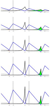
Refer to caption
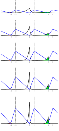
Refer to caption
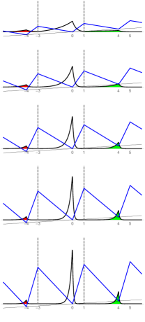
Refer to caption

(a𝑎a) κ=κ0/2𝜅subscript𝜅02\kappa=-\kappa_{0}/2                   (b𝑏b) κ=0𝜅0\kappa=0                       (c𝑐c) κ=κ0/2𝜅subscript𝜅02\kappa=\kappa_{0}/2

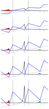
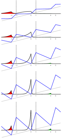
Figure 2: A Brownian motion with drift κ𝜅-\kappa, starting at 0, runs for time τ1=2.4subscript𝜏12.4\tau_{1}=2.4. Then, starting from where the Brownian motion ended, a tilted Brownian ratchet with α=1/4𝛼14\alpha=1/4, L=4𝐿4L=4, γ=λ(1α)/2𝛾𝜆1𝛼2\gamma=\lambda(1-\alpha)/2, λ=1,2,3,4,5𝜆12345\lambda=1,2,3,4,5 (from top to bottom), and κ=θκ0/2𝜅𝜃subscript𝜅02\kappa=\theta\kappa_{0}/2, κ0=0.2748subscript𝜅00.2748\kappa_{0}=0.2748, θ=1,0,1,2,3,4𝜃101234\theta=-1,0,1,2,3,4 (from left to right), runs for time τ2=2.4subscript𝜏22.4\tau_{2}=2.4. The black curve is an approximation to the density of the tilted flashing Brownian ratchet at time τ1+τ2subscript𝜏1subscript𝜏2\tau_{1}+\tau_{2}, via the improved random walk approximation with n=100𝑛100n=100. The blue curve is the sawtooth potential γV𝛾𝑉\gamma V (not just V𝑉V as in [4]), tilted with slope κ𝜅\kappa, then shrunk vertically by a factor of L𝐿L for clarity. (See the paragraph below (20) for the meaning of κ0subscript𝜅0\kappa_{0}.)
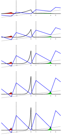
Refer to caption
Refer to caption
Refer to caption

(d𝑑d) κ=κ0𝜅subscript𝜅0\kappa=\kappa_{0}                     (e𝑒e) κ=3κ0/2𝜅3subscript𝜅02\kappa=3\kappa_{0}/2                     (f𝑓f) κ=2κ0𝜅2subscript𝜅0\kappa=2\kappa_{0}

Figure 2: (Continued) A Brownian motion with drift κ𝜅-\kappa, starting at 0, runs for time τ1=2.4subscript𝜏12.4\tau_{1}=2.4. Then, starting from where the Brownian motion ended, a tilted Brownian ratchet with α=1/4𝛼14\alpha=1/4, L=4𝐿4L=4, γ=λ(1α)/2𝛾𝜆1𝛼2\gamma=\lambda(1-\alpha)/2, λ=1,2,3,4,5𝜆12345\lambda=1,2,3,4,5 (from top to bottom), and κ=θκ0/2𝜅𝜃subscript𝜅02\kappa=\theta\kappa_{0}/2, κ0=0.2748subscript𝜅00.2748\kappa_{0}=0.2748, θ=1,0,1,2,3,4𝜃101234\theta=-1,0,1,2,3,4 (from left to right), runs for time τ2=2.4subscript𝜏22.4\tau_{2}=2.4. The black curve is an approximation to the density of the tilted flashing Brownian ratchet at time τ1+τ2subscript𝜏1subscript𝜏2\tau_{1}+\tau_{2}, via the improved random walk approximation with n=100𝑛100n=100. The blue curve is the sawtooth potential γV𝛾𝑉\gamma V (not just V𝑉V as in [4]), tilted with slope κ𝜅\kappa, then shrunk vertically by a factor of L𝐿L for clarity.

Before commenting on these figures, we observe that they could also have been derived using the methods of Sections 3 (Theorem 2), 4 (Theorem 4), or 5. However, stochastic simulation (Section 4) provides slightly less smooth figures in a comparable amount of time. For numerical solution of the Fokker–Planck equation (Section 5), recursion (19) and (20) with p0subscript𝑝0p_{0} and p1subscript𝑝1p_{1} as in (14) is identical with recursion (5) when γ=λ(1α)/2𝛾𝜆1𝛼2\gamma=\lambda(1-\alpha)/2. Thus, the method of Section 5 gives results identical to the improved random walk approximation of Section 3 (Theorem 2).

This observation is not entirely new. The main conclusion of Allison and Abbott [14] as well as Toral et al. [15, 16] is that, if the Fokker–Planck equation for the Brownian ratchet is suitably discretized, one gets an equation that is identical to the master equation for Parrondo’s capital-dependent game B𝐵B, at least for a suitable potential. A similar result was found by Heath et al. [17]. What is new in our approach is that we recover the specific potential in the definition of the Brownian ratchet. This requires not just letting ΔtΔ𝑡\Delta t and ΔyΔ𝑦\Delta y in the finite-difference method go to zero with (Δy)2/ΔtsuperscriptΔ𝑦2Δ𝑡(\Delta y)^{2}/\Delta t constant, but also requires letting the probabilities in the Parrondo games go to 1/2121/2 in a very specific way, unlike in the earlier works where these probabilities were fixed.

We computed statistics for the n𝑛nth random walk approximation (improved and unimproved) of the tilted flashing Brownian ratchet with α=1/4𝛼14\alpha=1/4, L=4𝐿4L=4, γ=λ(1α)/2𝛾𝜆1𝛼2\gamma=\lambda(1-\alpha)/2, λ=5𝜆5\lambda=5, κ=κ0=0.2748𝜅subscript𝜅00.2748\kappa=\kappa_{0}=0.2748, τ1=τ2=2.4subscript𝜏1subscript𝜏22.4\tau_{1}=\tau_{2}=2.4, and initial state 0, at time τ1+τ2subscript𝜏1subscript𝜏2\tau_{1}+\tau_{2}, for n=10,20,30,,200𝑛102030200n=10,20,30,\ldots,200. The rate of convergence using the improved approximation appeared notably faster. We omit these tables to save space.

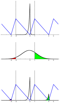
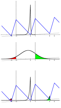
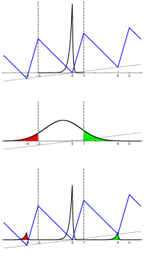
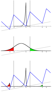
Although the conceptual figures in panels (c𝑐c) and (f𝑓f) of Figure 1 are largely accurate, the figures of Figure 2 offer several key improvements, just as we found in the untilted case. First, the three peaks of the density are pointed, unlike a normal density. Second, they are asymmetric, again unlike a normal density, with more mass to the left than to the right of 44-4, 0, and 4. This is largely due to the fact that, for example, the drift to the left on (0,1)01(0,1) is stronger than the drift to the right on (3,0)30(-3,0), but there also seems to be some dependence on the slope of the tilt. Third, the relative heights of the peaks vary more than in the conceptual figure. The simulations cited previously had implicitly noted the pointed [19] and asymmetric [19, 11] peaks.

The peaks in Figure 1 appear to be normal, while the peaks in Astumian and Hänggi  [6, Fig. 2] are explicitly called “gaussians.” This thinking led Astumian [5] to conclude that mean displacement at time τ1+τ2subscript𝜏1subscript𝜏2\tau_{1}+\tau_{2} has the form

j=jLPjL,where PjL:=P(Bτ1κτ1((j1+α)L,(j+α)L]).assignsuperscriptsubscript𝑗𝑗𝐿subscript𝑃𝑗𝐿where subscript𝑃𝑗𝐿Psubscript𝐵subscript𝜏1𝜅subscript𝜏1𝑗1𝛼𝐿𝑗𝛼𝐿\sum_{j=-\infty}^{\infty}jL\,P_{jL},\quad\text{where }P_{jL}:={\rm P}(B_{\tau_{1}}-\kappa\tau_{1}\in((j-1+\alpha)L,(j+\alpha)L]).

This is inaccurate for two reasons. Most importantly, the mean of the peak at jL𝑗𝐿jL is not jL𝑗𝐿jL because of the skewed nature of that peak. Also, the area of the peak at jL𝑗𝐿jL is not the normal probability PjLsubscript𝑃𝑗𝐿P_{jL}; this is only an approximation that becomes exact in the limit as γ𝛾\gamma\to\infty.

We consider a statistic that measures the skewness of the peaks of the distribution. The skewness can be defined to be the mass of the distribution in n=(nL,nL+αL)superscriptsubscript𝑛𝑛𝐿𝑛𝐿𝛼𝐿\bigcup_{n=-\infty}^{\infty}(nL,nL+\alpha L) minus the mass of the distribution in n=(nL(1α)L,nL)superscriptsubscript𝑛𝑛𝐿1𝛼𝐿𝑛𝐿\bigcup_{n=-\infty}^{\infty}(nL-(1-\alpha)L,nL). A negative skewness means that the peaks are skewed to the left.

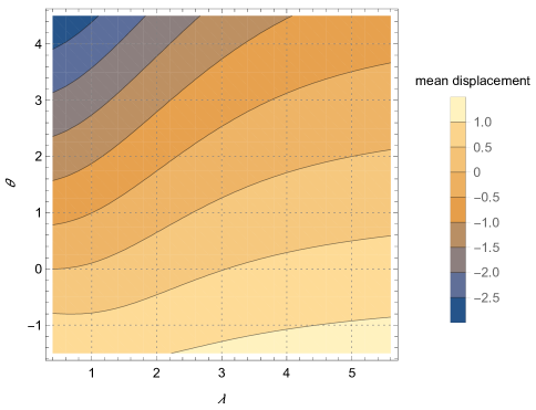
Table 1 shows the effect of varying κ𝜅\kappa, when λ=5𝜆5\lambda=5, on several statistics of interest, namely areas and heights of the three peaks, mean displacement, and skewness. Figure 3 shows that the mean displacement for the n𝑛nth improved random walk (n=100𝑛100n=100) approximating the tilted flashing Brownian ratchet, starting at 0, is increasing in γ𝛾\gamma and decreasing in κ𝜅\kappa. In fact, it decreases nearly linearly in κ𝜅\kappa.

Table 1: Computations for the n𝑛nth improved random walk (n=100𝑛100n=100) approximating the tilted flashing Brownian ratchet with α=1/4𝛼14\alpha=1/4, L=4𝐿4L=4, γ=λ(1α)/2𝛾𝜆1𝛼2\gamma=\lambda(1-\alpha)/2, λ=5𝜆5\lambda=5, κ=θκ0/2𝜅𝜃subscript𝜅02\kappa=\theta\kappa_{0}/2 for κ0=0.2748subscript𝜅00.2748\kappa_{0}=0.2748 and various θ𝜃\theta, τ1=τ2=2.4subscript𝜏1subscript𝜏22.4\tau_{1}=\tau_{2}=2.4, and initial state 0, at time τ1+τ2subscript𝜏1subscript𝜏2\tau_{1}+\tau_{2}, illustrating the effect of varying the slope of the tilt. (See the paragraph below (20) for the meaning of κ0subscript𝜅0\kappa_{0}.)
θ𝜃\theta areas of the three peaks heights of the three peaks mean skewness
[at 4,0,4404-4,0,4] displace.
1.51.5-1.5 (0.01521,0.6381,0.3466)0.015210.63810.3466(0.01521,0.6381,0.3466) (0.05597,2.348,1.269)0.055972.3481.269(0.05597,2.348,1.269)\hphantom{0} -1.21000 0.49300.4930-0.4930
1.01.0-1.0 (0.01995,0.6727,0.3074)0.019950.67270.3074(0.01995,0.6727,0.3074) (0.07215,2.433,1.107)0.072152.4331.107(0.07215,2.433,1.107)\hphantom{0} -1.02700 0.50620.5062-0.5062
0.50.5-0.5 (0.02588,0.7040,0.2701)0.025880.70400.2701(0.02588,0.7040,0.2701) (0.09197,2.501,0.9563)0.091972.5010.9563(0.09197,2.501,0.9563) -0.84740 0.51940.5194-0.5194
-0.0 (0.03324,0.7314,0.2353)0.033240.73140.2353(0.03324,0.7314,0.2353) (0.1159,2.551,0.8178)0.11592.5510.8178(0.1159,2.551,0.8178)\hphantom{0} -0.67160 0.53250.5325-0.5325
-0.5 (0.04225,0.7547,0.2031)0.042250.75470.2031(0.04225,0.7547,0.2031) (0.1445,2.581,0.6921)0.14452.5810.6921(0.1445,2.581,0.6921)\hphantom{0} -0.49950 0.54570.5457-0.5457
-1.0 (0.05317,0.7732,0.1736)0.053170.77320.1736(0.05317,0.7732,0.1736) (0.1782,2.591,0.5796)0.17822.5910.5796(0.1782,2.591,0.5796)\hphantom{0} -0.33080 0.55890.5589-0.5589
-1.5 (0.06622,0.7868,0.1470)0.066220.78680.1470(0.06622,0.7868,0.1470) (0.2173,2.580,0.4801)0.21732.5800.4801(0.2173,2.580,0.4801)\hphantom{0} -0.16460 0.57210.5721-0.5721
-2.0 (0.08166,0.7951,0.1233)0.081660.79510.1233(0.08166,0.7951,0.1233) (0.2620,2.549,0.3933)0.26202.5490.3933(0.2620,2.549,0.3933)\hphantom{0} -0.00002 0.58530.5853-0.5853
-2.5 (0.09970,0.7980,0.1023)0.099700.79800.1023(0.09970,0.7980,0.1023) (0.3125,2.499,0.3185)0.31252.4990.3185(0.3125,2.499,0.3185)\hphantom{0} 0.16430.1643-0.16430 0.59850.5985-0.5985
-3.0 (0.1205,0.7954,0.08405)0.12050.79540.08405(0.1205,0.7954,0.08405) (0.3687,2.429,0.2549)0.36872.4290.2549(0.3687,2.429,0.2549)\hphantom{0} 0.32960.3296-0.32960 0.61170.6117-0.6117
-3.5 (0.1443,0.7873,0.06834)0.14430.78730.06834(0.1443,0.7873,0.06834) (0.4302,2.342,0.2016)0.43022.3420.2016(0.4302,2.342,0.2016)\hphantom{0} 0.49710.4971-0.49710 0.62500.6250-0.6250
-4.0 (0.1711,0.7739,0.05498)0.17110.77390.05498(0.1711,0.7739,0.05498) (0.4965,2.238,0.1574)0.49652.2380.1574(0.4965,2.238,0.1574)\hphantom{0} 0.66820.6682-0.66820 0.63830.6383-0.6383
-4.5 (0.2010,0.7553,0.04376)0.20100.75530.04376(0.2010,0.7553,0.04376) (0.5668,2.121,0.1214)0.56682.1210.1214(0.5668,2.121,0.1214)\hphantom{0} 0.84390.8439-0.84390 0.65160.6516-0.6516
20.0000012800.000001280-0.000001280
Refer to caption
Figure 3: Mean displacement for the n𝑛nth improved random walk (n=100𝑛100n=100) approximating the tilted flashing Brownian ratchet with α=1/4𝛼14\alpha=1/4, L=4𝐿4L=4, γ=λ(1α)/2𝛾𝜆1𝛼2\gamma=\lambda(1-\alpha)/2, κ=θκ0/2𝜅𝜃subscript𝜅02\kappa=\theta\kappa_{0}/2, κ0=0.2748subscript𝜅00.2748\kappa_{0}=0.2748, τ1=τ2=2.4subscript𝜏1subscript𝜏22.4\tau_{1}=\tau_{2}=2.4, and initial state 0, at time τ1+τ2subscript𝜏1subscript𝜏2\tau_{1}+\tau_{2}, as a function of λ𝜆\lambda and θ𝜃\theta.

In particular, let us define κ0(λ)subscript𝜅0𝜆\kappa_{0}(\lambda) to be such that the contour with mean displacement 0 passes through (λ,κ0(λ))𝜆subscript𝜅0𝜆(\lambda,\kappa_{0}(\lambda)). For example, κ0(5)=0.2748subscript𝜅050.2748\kappa_{0}(5)=0.2748 to four significant digits. Figure 3 shows that κ0(λ)subscript𝜅0𝜆\kappa_{0}(\lambda) increases in λ𝜆\lambda. It appears that κ0(λ)5/12subscript𝜅0𝜆512\kappa_{0}(\lambda)\to 5/12 as λ𝜆\lambda\to\infty. More generally,

κ0(λ)(12α)Lτ1asλ.formulae-sequencesubscript𝜅0𝜆12𝛼𝐿subscript𝜏1as𝜆\kappa_{0}(\lambda)\to\frac{\big{(}\frac{1}{2}-\alpha\big{)}L}{\tau_{1}}\quad\text{as}\quad\lambda\to\infty.

Indeed, we expect that limλκ0(λ)subscript𝜆subscript𝜅0𝜆\lim_{\lambda\to\infty}\kappa_{0}(\lambda) is the value of κ𝜅\kappa that makes P(Yτ1αL)=P(Yτ1<(1α)L)Psubscript𝑌subscript𝜏1𝛼𝐿Psubscript𝑌subscript𝜏11𝛼𝐿{\rm P}(Y_{\tau_{1}}\geq\alpha L)={\rm P}(Y_{\tau_{1}}<-(1-\alpha)L). But Yτ1=Bτ1κτ1subscript𝑌subscript𝜏1subscript𝐵subscript𝜏1𝜅subscript𝜏1Y_{\tau_{1}}=B_{\tau_{1}}-\kappa\tau_{1}, so κ𝜅\kappa must satisfy κτ1+αL=[κτ1(1α)L]𝜅subscript𝜏1𝛼𝐿delimited-[]𝜅subscript𝜏11𝛼𝐿\kappa\tau_{1}+\alpha L=-[\kappa\tau_{1}-(1-\alpha)L], and the conclusion follows. This result is due to Astumian [5].

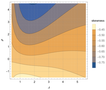
Figure 4 (also Table 1) shows that the absolute value of the skewness for the n𝑛nth improved random walk (n=100𝑛100n=100) approximating the tilted flashing Brownian ratchet, starting at 0, is increasing in κ𝜅\kappa.

Refer to caption
Figure 4: Skewness for the n𝑛nth improved random walk (n=100𝑛100n=100) approximating the tilted flashing Brownian ratchet with α=1/4𝛼14\alpha=1/4, L=4𝐿4L=4, γ=λ(1α)/2𝛾𝜆1𝛼2\gamma=\lambda(1-\alpha)/2, κ=θκ0/2𝜅𝜃subscript𝜅02\kappa=\theta\kappa_{0}/2, κ0=0.2748subscript𝜅00.2748\kappa_{0}=0.2748, τ1=τ2=2.4subscript𝜏1subscript𝜏22.4\tau_{1}=\tau_{2}=2.4, and initial state 0, at time τ1+τ2subscript𝜏1subscript𝜏2\tau_{1}+\tau_{2}, as a function of λ𝜆\lambda and θ𝜃\theta.

7 Density at time τ1+τ2subscript𝜏1subscript𝜏2\tau_{1}+\tau_{2}, starting at stationarity

We may want to wrap the tilted Brownian ratchet and the tilted flashing Brownian ratchet around the circle of circumference L𝐿L. By virtue of the fact that their behavior is spatially periodic with period L𝐿L, the wrapped processes remain Markovian. We define the wrapped tilted Brownian ratchet as the [0,L)0𝐿[0,L)-valued process

X¯t:=mod(Xt,L),assignsubscript¯𝑋𝑡modsubscript𝑋𝑡𝐿\bar{X}_{t}:=\text{mod}(X_{t},L),

where Xtsubscript𝑋𝑡X_{t} denotes the tilted Brownian ratchet in (3), with the understanding that the endpoints of the interval [0,L)0𝐿[0,L) are identified, making it a circle of circumference L𝐿L. The same procedure yields the wrapped tilted flashing Brownian ratchet,

Y¯t:=mod(Yt,L),assignsubscript¯𝑌𝑡modsubscript𝑌𝑡𝐿\bar{Y}_{t}:=\text{mod}(Y_{t},L),

where Ytsubscript𝑌𝑡Y_{t} denotes the tilted flashing Brownian ratchet in (6). Note that the skewness, as it was defined in the preceding section, can be determined for the original processes from the wrapped processes. The same is not true for the mean displacement.

We begin by finding the stationary distribution of the wrapped tilted Brownian ratchet. This process is a diffusion process in [0,L]0𝐿[0,L] (endpoints are identified) with generator

(f)(x):=12f′′(x)+μ(x)f(x).assign𝑓𝑥12superscript𝑓′′𝑥𝜇𝑥superscript𝑓𝑥(\mathscr{L}f)(x):=\frac{1}{2}f^{\prime\prime}(x)+\mu(x)f^{\prime}(x).

To begin, let us assume that μ𝜇\mu is a smooth function with μ(0)=μ(L)𝜇0𝜇𝐿\mu(0)=\mu(L). We hope that, once we have the desired formula, we can substitute the actual μ𝜇\mu, namely (2), which has discontinuities.

We want to find the function ϕitalic-ϕ\phi satisfying

0L(f)(x)ϕ(x)𝑑x=0,superscriptsubscript0𝐿𝑓𝑥italic-ϕ𝑥differential-d𝑥0\int_{0}^{L}(\mathscr{L}f)(x)\phi(x)\,dx=0,

ϕ(0)=ϕ(L)italic-ϕ0italic-ϕ𝐿\phi(0)=\phi(L), and ϕ(0)=ϕ(L)superscriptitalic-ϕ0superscriptitalic-ϕ𝐿\phi^{\prime}(0)=\phi^{\prime}(L) for all smooth f𝑓f with f(0)=f(L)𝑓0𝑓𝐿f(0)=f(L) and f(0)=f(L)superscript𝑓0superscript𝑓𝐿f^{\prime}(0)=f^{\prime}(L). We expect that

0L(f)(x)ϕ(x)𝑑x=0Lf(x)(ϕ)(x)𝑑x,superscriptsubscript0𝐿𝑓𝑥italic-ϕ𝑥differential-d𝑥superscriptsubscript0𝐿𝑓𝑥superscriptitalic-ϕ𝑥differential-d𝑥\int_{0}^{L}(\mathscr{L}f)(x)\phi(x)\,dx=\int_{0}^{L}f(x)(\mathscr{L}^{*}\phi)(x)\,dx, (21)

where

(ϕ)(x):=12ϕ′′(x)(μϕ)(x)assignsuperscriptitalic-ϕ𝑥12superscriptitalic-ϕ′′𝑥superscript𝜇italic-ϕ𝑥(\mathscr{L}^{*}\phi)(x):=\frac{1}{2}\phi^{\prime\prime}(x)-(\mu\phi)^{\prime}(x)

is the formal adjoint of \mathscr{L}, showing that it suffices to solve the differential equation

(ϕ)(x)=0.superscriptitalic-ϕ𝑥0(\mathscr{L}^{*}\phi)(x)=0. (22)

The justification of (21) requires three integrations by parts and f(0)=f(L)𝑓0𝑓𝐿f(0)=f(L), f(0)=f(L)superscript𝑓0superscript𝑓𝐿f^{\prime}(0)=f^{\prime}(L), ϕ(0)=ϕ(L)italic-ϕ0italic-ϕ𝐿\phi(0)=\phi(L), ϕ(0)=ϕ(L)superscriptitalic-ϕ0superscriptitalic-ϕ𝐿\phi^{\prime}(0)=\phi^{\prime}(L), and μ(0)=μ(L)𝜇0𝜇𝐿\mu(0)=\mu(L).

It remains to solve the differential equation (22), which is equivalent to

12ϕ(x)μ(x)ϕ(x)=C,ϕ(0)=ϕ(L),ϕ(0)=ϕ(L),formulae-sequence12superscriptitalic-ϕ𝑥𝜇𝑥italic-ϕ𝑥𝐶formulae-sequenceitalic-ϕ0italic-ϕ𝐿superscriptitalic-ϕ0superscriptitalic-ϕ𝐿\frac{1}{2}\phi^{\prime}(x)-\mu(x)\phi(x)=C,\qquad\phi(0)=\phi(L),\quad\phi^{\prime}(0)=\phi^{\prime}(L),

for some constant C𝐶C. Letting

M(x):=0xμ(y)𝑑y,assign𝑀𝑥superscriptsubscript0𝑥𝜇𝑦differential-d𝑦M(x):=\int_{0}^{x}\mu(y)\,dy,

we find using elementary methods that

ϕ(x)=ϕ(0)e2M(x)(1[1e2M(L)]0xe2M(y)𝑑y0Le2M(y)𝑑y).italic-ϕ𝑥italic-ϕ0superscript𝑒2𝑀𝑥1delimited-[]1superscript𝑒2𝑀𝐿superscriptsubscript0𝑥superscript𝑒2𝑀𝑦differential-d𝑦superscriptsubscript0𝐿superscript𝑒2𝑀𝑦differential-d𝑦\phi(x)=\phi(0)e^{2M(x)}\bigg{(}1-\big{[}1-e^{-2M(L)}\big{]}\frac{\int_{0}^{x}e^{-2M(y)}\,dy}{\int_{0}^{L}e^{-2M(y)}\,dy}\bigg{)}. (23)

The solution is unique, once we require that

0Lϕ(x)𝑑x=1.superscriptsubscript0𝐿italic-ϕ𝑥differential-d𝑥1\int_{0}^{L}\phi(x)\,dx=1.

Now we can use this result with the desired μ𝜇\mu, even though μ𝜇\mu has discontinuities. Specifically, with

M(x)=[γV(x)+κx],𝑀𝑥delimited-[]𝛾𝑉𝑥𝜅𝑥M(x)=-[\gamma V(x)+\kappa x], (24)

we have an analytical formula for ϕitalic-ϕ\phi, which can be shown to be equivalent to a formula of Reimann [7, Eq. (2.36)].

Theorem 5 (Stationary distribution of the wrapped tilted Brownian ratchet).

The wrapped tilted Brownian ratchet with parameters α𝛼\alpha, L𝐿L, γ𝛾\gamma, and κ𝜅\kappa has a stationary distribution π𝜋\pi of the form (23) (((using (24)))), restricted to [0,L]0𝐿[0,L].

The skewness of this stationary distribution can be evaluated. In the special case κ=0𝜅0\kappa=0, the computation is especially easy and we find that the skewness is 2α12𝛼12\alpha-1; surprisingly, it does not depend on γ𝛾\gamma.

We denote the tilted flashing Brownian ratchet at time t𝑡t, starting from x𝐑𝑥𝐑x\in{\bf R} at time 0, by Ytxsuperscriptsubscript𝑌𝑡𝑥Y_{t}^{x}, and the wrapped tilted flashing Brownian ratchet at time t𝑡t, starting from x[0,L)𝑥0𝐿x\in[0,L) at time 0, by Y¯txsuperscriptsubscript¯𝑌𝑡𝑥\bar{Y}_{t}^{x}. Then the one-step transition function

P¯(x,):=P(Y¯τ1+τ2x)assign¯𝑃𝑥Psuperscriptsubscript¯𝑌subscript𝜏1subscript𝜏2𝑥\bar{P}(x,\cdot):={\rm P}(\bar{Y}_{\tau_{1}+\tau_{2}}^{x}\in\cdot) (25)

for a continuous-state Markov chain has a stationary distribution π¯¯𝜋\bar{\pi}. The mean displacement μ¯¯𝜇\bar{\mu} of the tilted flashing Brownian ratchet over the time interval [0,τ1+τ2]0subscript𝜏1subscript𝜏2[0,\tau_{1}+\tau_{2}], starting from the stationary distribution π¯¯𝜋\bar{\pi}, namely

μ¯¯𝜇\displaystyle\bar{\mu} :=0LE[Yτ1+τ2xY0x]π¯(dx)assignabsentsuperscriptsubscript0𝐿Edelimited-[]superscriptsubscript𝑌subscript𝜏1subscript𝜏2𝑥superscriptsubscript𝑌0𝑥¯𝜋𝑑𝑥\displaystyle:=\int_{0}^{L}{\rm E}[Y_{\tau_{1}+\tau_{2}}^{x}-Y_{0}^{x}]\,\bar{\pi}(dx)
=(1α)LαLE[Yτ1+τ2xY0x]π¯(dx)absentsuperscriptsubscript1𝛼𝐿𝛼𝐿Edelimited-[]superscriptsubscript𝑌subscript𝜏1subscript𝜏2𝑥superscriptsubscript𝑌0𝑥¯𝜋𝑑𝑥\displaystyle\phantom{:}=\int_{-(1-\alpha)L}^{\alpha L}{\rm E}[Y_{\tau_{1}+\tau_{2}}^{x}-Y_{0}^{x}]\,\bar{\pi}(dx)

is of interest. The second equality is based on the periodicity of the integrand (with period L𝐿L) and the convention that we do not distinguish notationally between π¯¯𝜋\bar{\pi} and its image under the mapping

x{xif 0x<αL,xLif αLx<L.maps-to𝑥cases𝑥if 0x<αL,𝑥𝐿if αLx<L.x\mapsto\begin{cases}x&\text{if $0\leq x<\alpha L$,}\\ x-L&\text{if $\alpha L\leq x<L$.}\end{cases}

We approximate μ¯¯𝜇\bar{\mu} as follows. The integrand can be estimated as in Section 6, the only distinction being that the starting point of the tilted flashing Brownian ratchet is x𝑥x, not 0. The stationary distribution π¯¯𝜋\bar{\pi} of the one-step transition function (25) can be approximated by the stationary distribution of the finite Markov chain whose one-step transition matrix has the form

P(i,j):=P(Y¯n(n2(τ1+τ2))=jY¯n(0)=i),i,j=0,1,,nL1,formulae-sequenceassign𝑃𝑖𝑗Psubscript¯𝑌𝑛superscript𝑛2subscript𝜏1subscript𝜏2conditional𝑗subscript¯𝑌𝑛0𝑖𝑖𝑗01𝑛𝐿1P(i,j):={\rm P}(\bar{Y}_{n}(n^{2}(\tau_{1}+\tau_{2}))=j\mid\bar{Y}_{n}(0)=i),\quad i,j=0,1,\ldots,nL-1,

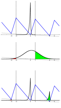
where {Y¯n(k),k=0,1,}formulae-sequencesubscript¯𝑌𝑛𝑘𝑘01\{\bar{Y}_{n}(k),\,k=0,1,\ldots\} denotes the wrapped (period-nL𝑛𝐿nL) random walk used to approximate the wrapped tilted flashing Brownian ratchet. A minor technical issue, if nL𝑛𝐿nL is even, is that this Markov chain fails to be irreducible if n2(τ1+τ2)superscript𝑛2subscript𝜏1subscript𝜏2n^{2}(\tau_{1}+\tau_{2}) is even, in which case we replace n2(τ1+τ2)superscript𝑛2subscript𝜏1subscript𝜏2n^{2}(\tau_{1}+\tau_{2}) by n2(τ1+τ2)+1superscript𝑛2subscript𝜏1subscript𝜏21n^{2}(\tau_{1}+\tau_{2})+1. Then the chain is irreducible and there is a unique stationary distribution. The black curve in the first row of the panels in Figure 5 approximates the density of π¯¯𝜋\bar{\pi} with support [3,1)31[-3,1). Starting from the approximate π¯¯𝜋\bar{\pi} at time 0, the black curves in the second and third rows of each panel are the approximations to the density of the tilted flashing Brownian ratchet at times τ1subscript𝜏1\tau_{1} and τ1+τ2subscript𝜏1subscript𝜏2\tau_{1}+\tau_{2}, respectively. When λ=5𝜆5\lambda=5 and κ=κ0=0.2748𝜅subscript𝜅00.2748\kappa=\kappa_{0}=0.2748, computations show that μ¯=0.01519¯𝜇0.01519\bar{\mu}=0.01519, which is slightly larger than the corresponding number in Table 1, namely 0.0000. A more complete set of such computations is given as Table 2. It is interesting to compare this table (starting at stationarity) with Table 1 (starting at 0).
Refer to caption
Refer to caption
Refer to caption

(a𝑎a) κ=κ0/2𝜅subscript𝜅02\kappa=-\kappa_{0}/2                   (b𝑏b) κ=0𝜅0\kappa=0                       (c𝑐c) κ=κ0/2𝜅subscript𝜅02\kappa=\kappa_{0}/2
Refer to caption Refer to caption Refer to caption
(d𝑑d) κ=κ0𝜅subscript𝜅0\kappa=\kappa_{0}                     (e𝑒e) κ=3κ0/2𝜅3subscript𝜅02\kappa=3\kappa_{0}/2                     (f𝑓f) κ=2κ0𝜅2subscript𝜅0\kappa=2\kappa_{0}

Figure 5: Starting from the stationary distribution π¯¯𝜋\bar{\pi} with support [3,1)31[-3,1), a Brownian motion with drift κ𝜅-\kappa runs for time τ1=2.4subscript𝜏12.4\tau_{1}=2.4. Then, starting from where the Brownian motion ended, a tilted Brownian ratchet with α=1/4𝛼14\alpha=1/4, L=4𝐿4L=4, γ=λ(1α)/2𝛾𝜆1𝛼2\gamma=\lambda(1-\alpha)/2, λ=5𝜆5\lambda=5, and κ=θκ0/2𝜅𝜃subscript𝜅02\kappa=\theta\kappa_{0}/2, κ0=0.2748subscript𝜅00.2748\kappa_{0}=0.2748 (with θ=1,0,1,2,3,4𝜃101234\theta=-1,0,1,2,3,4), runs for time τ2=2.4subscript𝜏22.4\tau_{2}=2.4. The black curves approximate the density of the tilted flashing Brownian ratchet at times 0, τ1subscript𝜏1\tau_{1}, and τ2+τ2subscript𝜏2subscript𝜏2\tau_{2}+\tau_{2}, via the improved random walk approximation with n=100𝑛100n=100. The blue curves are as in Figure 2. The vertical axes in the panels of the first and third rows are comparable, whereas the vertical axis in the panels of the second row (for the normal-like curve but not for the tilted axis) has been stretched by a factor of L𝐿L for clarity.
Table 2: Computations for the n𝑛nth improved random walk (n=100𝑛100n=100) approximating the tilted flashing Brownian ratchet with α=1/4𝛼14\alpha=1/4, L=4𝐿4L=4, γ=λ(1α)/2𝛾𝜆1𝛼2\gamma=\lambda(1-\alpha)/2, λ=5𝜆5\lambda=5, κ=θκ0/2𝜅𝜃subscript𝜅02\kappa=\theta\kappa_{0}/2 for κ0=0.2748subscript𝜅00.2748\kappa_{0}=0.2748 and various θ𝜃\theta, and τ1=τ2=2.4subscript𝜏1subscript𝜏22.4\tau_{1}=\tau_{2}=2.4, starting at stationarity, at time τ1+τ2subscript𝜏1subscript𝜏2\tau_{1}+\tau_{2}, illustrating the effect of varying the slope of the tilt. (See the paragraph below (20) for the meaning of κ0subscript𝜅0\kappa_{0}.)
θ𝜃\theta areas of the three peaks heights of the three peaks mean skewness
[at 4,0,4404-4,0,4] displace.
1.51.5-1.5 (0.01929,0.6609,0.3199)0.019290.66090.3199(0.01929,0.6609,0.3199) (0.07095,2.431,1.171)0.070952.4311.171(0.07095,2.431,1.171)\hphantom{0} -1.20700 0.49570.4957-0.4957
1.01.0-1.0 (0.02523,0.6936,0.2811)0.025230.69360.2811(0.02523,0.6936,0.2811) (0.09127,2.509,1.013)0.091272.5091.013(0.09127,2.509,1.013)\hphantom{0} -1.02700 0.50890.5089-0.5089
0.50.5-0.5 (0.03267,0.7226,0.2448)0.032670.72260.2448(0.03267,0.7226,0.2448) (0.1161,2.567,0.8666)0.11612.5670.8666(0.1161,2.567,0.8666)\hphantom{0} -0.85070 0.52200.5220-0.5220
-0.0 (0.04185,0.7471,0.2110)0.041850.74710.2110(0.04185,0.7471,0.2110) (0.1459,2.605,0.7336)0.14592.6050.7336(0.1459,2.605,0.7336)\hphantom{0} -0.67830 0.53520.5352-0.5352
-0.5 (0.05304,0.7668,0.1802)0.053040.76680.1802(0.05304,0.7668,0.1802) (0.1814,2.622,0.6141)0.18142.6220.6141(0.1814,2.622,0.6141)\hphantom{0} -0.50940 0.54830.5483-0.5483
-1.0 (0.06654,0.7812,0.1522)0.066540.78120.1522(0.06654,0.7812,0.1522) (0.2230,2.618,0.5082)0.22302.6180.5082(0.2230,2.618,0.5082)\hphantom{0} -0.34330 0.56150.5615-0.5615
-1.5 (0.08260,0.7901,0.1273)0.082600.79010.1273(0.08260,0.7901,0.1273) (0.2709,2.591,0.4157)0.27092.5910.4157(0.2709,2.591,0.4157)\hphantom{0} -0.17900 0.57460.5746-0.5746
-2.0 (0.1015,0.7932,0.1053)0.10150.79320.1053(0.1015,0.7932,0.1053)\hphantom{0} (0.3255,2.543,0.3360)0.32552.5430.3360(0.3255,2.543,0.3360)\hphantom{0} -0.01519 0.58780.5878-0.5878
-2.5 (0.1234,0.7904,0.08614)0.12340.79040.08614(0.1234,0.7904,0.08614) (0.3867,2.475,0.2682)0.38672.4750.2682(0.3867,2.475,0.2682)\hphantom{0} 0.14950.1495-0.14950 0.60100.6010-0.6010
-3.0 (0.1486,0.7817,0.06969)0.14860.78170.06969(0.1486,0.7817,0.06969) (0.4542,2.387,0.2113)0.45422.3870.2113(0.4542,2.387,0.2113)\hphantom{0} 0.31630.3163-0.31630 0.61420.6142-0.6142
-3.5 (0.1771,0.7672,0.05573)0.17710.76720.05573(0.1771,0.7672,0.05573) (0.5275,2.281,0.1644)0.52752.2810.1644(0.5275,2.281,0.1644)\hphantom{0} 0.48670.4867-0.48670 0.62740.6274-0.6274
-4.0 (0.2090,0.7470,0.04405)0.20900.74700.04405(0.2090,0.7470,0.04405) (0.6057,2.159,0.1261)0.60572.1590.1261(0.6057,2.159,0.1261)\hphantom{0} 0.66180.6618-0.66180 0.64070.6407-0.6407
-4.5 (0.2442,0.7214,0.03440)0.24420.72140.03440(0.2442,0.7214,0.03440) (0.6876,2.024,0.09540)0.68762.0240.09540(0.6876,2.024,0.09540) 0.84250.8425-0.84250 0.65390.6539-0.6539

8 Conclusions

A tilted flashing Brownian ratchet is a flashing Brownian ratchet in the presence of a static homogeneous force acting in the direction opposite that of the directed motion, thereby reducing (or reversing) the directed motion effect. We began by deriving a general class of capital-dependent Parrondo games with a bias parameter, motivated by the tilted Brownian ratchet. These Parrondo games, in turn, motivated our random walk approximation of the tilted flashing Brownian ratchet, which we subsequently improved. This is an efficient method of numerically approximating the distribution of a continuous process at a fixed time, more accurate than stochastic simulation (Section 4) but equivalent to numerical PDE analysis (Section 5). We found the approximate density of the tilted flashing Brownian ratchet after one time period, starting at 0. We also found the approximate density of the tilted flashing Brownian ratchet after the same time period, but now starting from a stationary distribution associated with the wrapped tilted flashing Brownian ratchet. In both cases the distributions are mixtures of asymmetric unimodal distributions, contrary to what was suggested by conceptual figures such as Figure 1. We approximated the mean displacement of the tilted flashing Brownian ratchet over that time period and observed that the mean displacement is increasing in γ𝛾\gamma, a measure of the amplitude of the potential, and decreasing in κ𝜅\kappa, the slope of tilt.

Acknowledgments

The work of S. N. Ethier was partially supported by a grant from the Simons Foundation (429675). The work of J. Lee was supported by the Basic Science Research Program through the National Research Foundation of Korea (NRF) funded by the Ministry of Education (NRF-2018R1D1A1B07042307).

References

  • [1] Ajdari A, Prost J. 1992 Drift induced by a spatially periodic potential of low symmetry: Pulsed dielectrophoresis. C. R. Acad. Sci., Série 2 315, 1635–1639.
  • [2] Harmer GP, Abbott D, Taylor PG. 2000 The paradox of Parrondo’s games. Proc. R. Soc. Lond. A 456, 247–259.
  • [3] Harmer GP, Abbott D. 1999 Parrondo’s paradox. Statist. Sci. 14, 206–213.
  • [4] Ethier SN, Lee J. 2018 The flashing Brownian ratchet and Parrondo’s paradox. R. Soc. Open Sci. 5, 171685.
  • [5] Astumian RD. 1997 Thermodynamics and kinetics of a Brownian motor. Science 276, 917–922.
  • [6] Astumian RD, Hänggi P. 2002 Brownian motors. Phys. Today 55 (11) 33–39.
  • [7] Reimann P. 2002 Brownian motors: noisy transport far from equilibrium. Phys. Rep. 361, 57–265.
  • [8] Reimann P, Hänggi P. 2002 Introduction to the physics of Brownian motors. Appl. Phys. A 75, 169–178.
  • [9] Parrondo JMR, de Cisneros BJ. 2002 Energetics of Brownian motors: a review. Appl. Phys. A 75, 179–191.
  • [10] Dinis [Vizcaíno] LI. 2006 Optimización y control de juegos de azar y motores brownianos colectivos. Doctoral Thesis, Universidad Complutense de Madrid, Spain.
  • [11] Hänggi P, Marchesoni F. 2009 Artificial Brownian motors: Controlling transport on the nanoscale, Rev. Mod. Phys. 81, 387–442.
  • [12] Harmer GP, Abbott D. 2002 A review of Parrondo’s paradox. Fluct. Noise Lett. 2, R71–R107.
  • [13] Harmer GP, Abbott D, Taylor PG, Parrondo JMR. 2001 Brownian ratchets and Parrondo’s games. Chaos 11, 705–714.
  • [14] Allison A, Abbott D. 2002 The physical basis for Parrondo’s games. Fluct. Noise Lett. 2, L327–L341.
  • [15] Toral R, Amengual P, Mangioni S. 2003 Parrondo’s games as a discrete ratchet. Physica A 327, 105–110.
  • [16] Toral R, Amengual P, Mangioni S. 2003 A Fokker–Planck description for Parrondo’s games. In Noise in Complex Systems and Stochastic Dynamics (eds L Schimansky-Geier, D Abbott, A Neiman, C van den Broeck). Proc. SPIE Series, vol. 5114, pp. 309–317. Bellingham, WA: Society of Photo-optical Instrumentation Engineers.
  • [17] Heath D, Kinderlehrer D, Kowalczyk M. 2002 Discrete and continuous ratchets: From coin toss to molecular motor. Discrete Contin. Dyn. Syst. B 2, 153–167.
  • [18] Ethier SN, Kurtz TG. Markov Processes: Characterization and Convergence Wiley, New York, 1986.
  • [19] Kinderlehrer D, Kowalczyk M. 2002 Diffusion-mediated transport and the flashing ratchet. Arch. Rational Mech. Anal. 161, 149–179.
  • [20] Mitchell AR, Griffiths DF. 1980 The Finite Difference Method in Partial Differential Equations. Wiley, New York.