Planck 2018 results. X. Constraints on inflation
We report on the implications for cosmic inflation of the 2018 release of the Planck cosmic microwave background (CMB) anisotropy measurements. The results are fully consistent with those reported using the data from the two previous Planck cosmological releases, but have smaller uncertainties thanks to improvements in the characterization of polarization at low and high multipoles. Planck temperature, polarization, and lensing data determine the spectral index of scalar perturbations to be at 68 % CL. We find no evidence for a scale dependence of , either as a running or as a running of the running. The Universe is found to be consistent with spatial flatness with a precision of at 95 % CL by combining Planck with a compilation of BAO data. The Planck 95 % CL upper limit on the tensor-to-scalar ratio, , is further tightened by combining with the BICEP2/Keck Array BK15 data to obtain . In the framework of standard single-field inflationary models with Einstein gravity, these results imply that: (a) the predictions of slow-roll models with a concave potential, , are increasingly favoured by the data; and (b) based on two different methods for reconstructing the inflaton potential, we find no evidence for dynamics beyond slow roll. Three different methods for the non-parametric reconstruction of the primordial power spectrum consistently confirm a pure power law in the range of comoving scales . A complementary analysis also finds no evidence for theoretically motivated parameterized features in the Planck power spectra. For the case of oscillatory features that are logarithmic or linear in this result is further strengthened by a new combined analysis including the Planck bispectrum data. The new Planck polarization data provide a stringent test of the adiabaticity of the initial conditions for the cosmological fluctuations. In correlated, mixed adiabatic and isocurvature models, the non-adiabatic contribution to the observed CMB temperature variance is constrained to 1.3 %, 1.7 %, and 1.7 % at 95 % CL for cold dark matter, neutrino density, and neutrino velocity, respectively. Planck power spectra plus lensing set constraints on the amplitude of compensated cold dark matter-baryon isocurvature perturbations that are consistent with current complementary measurements. The polarization data also provide improved constraints on inflationary models that predict a small statistically anisotropic quadupolar modulation of the primordial fluctuations. However, the polarization data do not support physical models for a scale-dependent dipolar modulation. All these findings support the key predictions of the standard single-field inflationary models, which will be further tested by future cosmological observations.
1 Introduction
This paper, one of a set associated with the 2018 release of data from the Planck111Planck (http://www.esa.int/Planck) is a project of the European Space Agency (ESA) with instruments provided by two scientific consortia funded by ESA member states and led by Principal Investigators from France and Italy, telescope reflectors provided through a collaboration between ESA and a scientific consortium led and funded by Denmark, and additional contributions from NASA (USA). mission, presents the implications for cosmic inflation of the 2018 Planck measurements of the cosmic microwave background (CMB) anisotropies. In terms of data, this paper updates Planck Collaboration XXII (2014) (henceforth PCI13), which was based on the temperature data of the nominal Planck mission (“PR1”), including the first 14 months of observations, and Planck Collaboration XX (2016) (henceforth PCI15), which used temperature data and a first set of polarization data from the full Planck mission (“PR2”), comprising 29 and 52 months of observations for the high frequency instrument (HFI) and low frequency instrument (LFI), respectively.
The ideas underlying cosmic inflation were developed during the late 1970s and early 1980s in order to remedy a number of defects of the hot big-bang cosmological model (e.g., the horizon, smoothness, flatness, and monopole problems) (Brout et al. 1978; Starobinsky 1980; Kazanas 1980; Sato 1981; Guth 1981; Linde 1982; Albrecht & Steinhardt 1982; Linde 1983). Subsequently, it was realized that, on account of quantum vacuum fluctuations, cosmic inflation also provides a means to generate the primordial cosmological perturbations (Mukhanov & Chibisov 1981, 1982; Hawking 1982; Guth & Pi 1982; Starobinsky 1982; Bardeen et al. 1983; Mukhanov 1985). The development of cosmic inflation is one of the major success stories of modern cosmology, and in this paper we explore how the latest 2018 release of the Planck data constrains inflationary models.
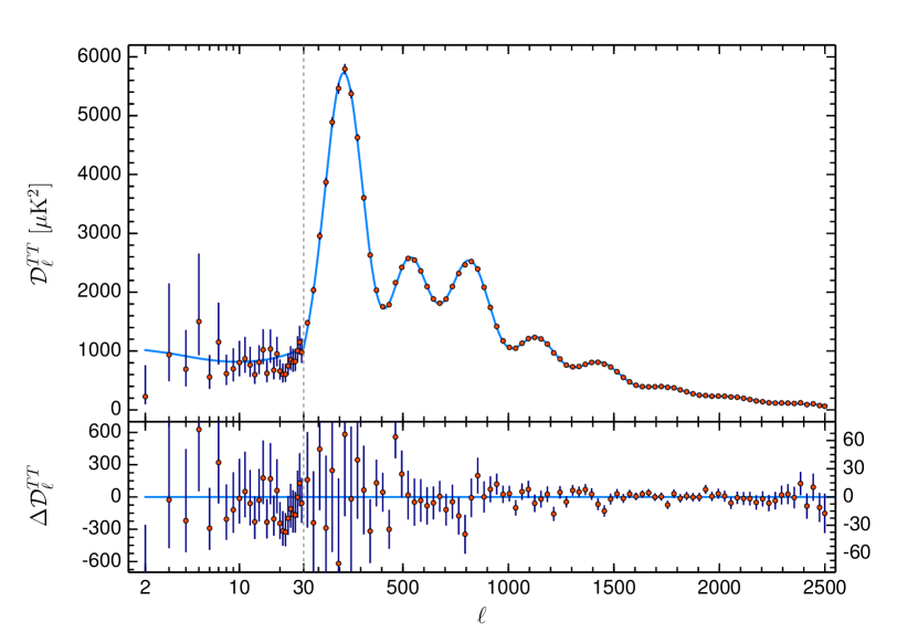
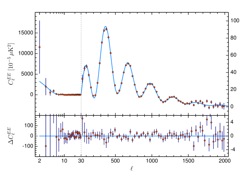
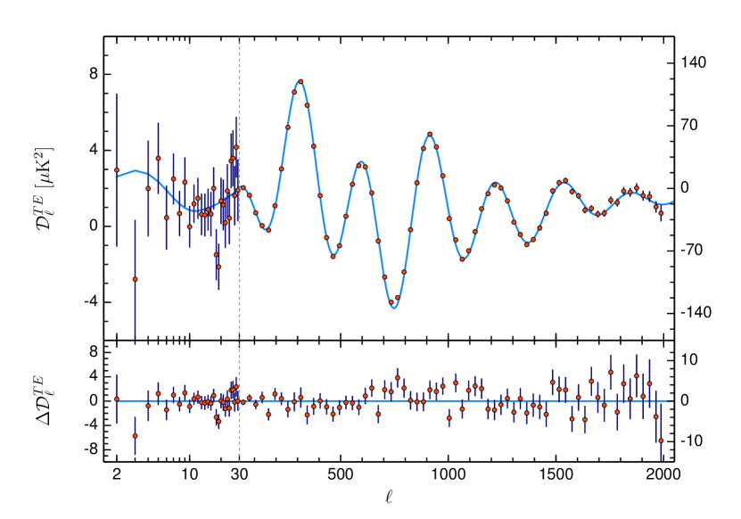
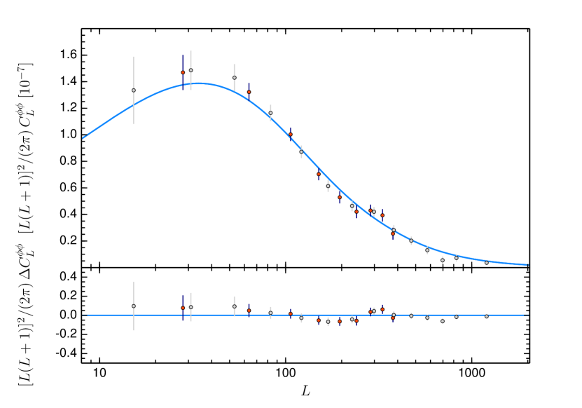
Planck data currently provide the best constraints on the CMB anisotropies, except on very small angular scales beyond the resolution limit of Planck. The Planck data set has enabled a precision characterization of the primordial cosmological perturbations and has allowed cosmological parameters to be constrained at the sub-percent level. One of the main data products, described in more detail in the following section, is the Planck , , , and lensing power spectra, which are shown in Fig. 1, together with the residuals from the six-parameter concordance cold dark matter (CDM) model using the best-fit parameter values.
In order to provide a quantitative estimate of the improvement achieved by Planck, as well as to show where Planck stands compared to an ultimate cosmic-variance-limited survey, we consider an idealistic estimator for the number of modes [i.e., the effective number of ’s measured (Planck Collaboration I 2016)]:
| (1) |
where () is the (error on the) angular power spectrum of the channel (Planck Collaboration I 2016; Scott et al. 2016). The number of modes measured by Planck is and for temperature ( up to ) and polarization ( up to ), respectively (Planck Collaboration I 2018). The number of modes measured is increased by approximately a factor of 7 (570) for temperature (polarization) with respect to the WMAP 9-year measurement, but there is still a factor of 3 (40) to gain for a cosmic-variance-limited experiment up to accessing 70 % of the sky. The additional modes measured by Planck play a key role in improving the constraints on the initial conditions for the cosmological perturbations and on models of inflation with respect to previous measurements of CMB anisotropies.
Planck data have also greatly improved the constraints on bispectral non-Gaussianity, both for the “local” pattern, as predicted by many inflationary models, and for other templates such as the equilateral one, as analysed and reported in detail in the dedicated Planck non-Gaussianity papers (Planck Collaboration XXIV 2014; Planck Collaboration XVII 2016; Planck Collaboration IX 2018). The constraints on the non-Gaussianity parameter are limited by a combination of cosmic variance and instrumental noise. An order-of-magnitude estimate for the signal-to-noise ratio for the local pattern (with ) is given by
| (2) |
For the local shape, the logarithm enters because most of the signal derives from detecting the modulation of the small-scale power by the large-scale CMB anisotropy, highlighting the importance of full-sky maps for this kind of analysis. For other shapes such as equilateral, one instead has . Planck has significantly sharpened the constraints on , largely on account of its measurement of high multipoles with higher signal-to-noise ratio compared to past surveys. Some improvement has also been obtained from including polarization.
The Planck measurements have significantly constrained the physics of inflation. The hypothesis of adiabatic Gaussian scalar fluctuations with a power spectrum described by a simple power law, which is the key prediction of the standard single-field slow-roll inflationary models, has been tested to unprecedent accuracy (\al@planck2013-p17,planck2014-a24; \al@planck2013-p17,planck2014-a24;Planck Collaboration XXIV 2014; Planck Collaboration XVII 2016). Planck has set tight constraints on the amount of inflationary gravitational waves by exploiting the shape of the CMB temperature spectrum (PCI13). These results have inspired a resurgence of activity in inflationary model building. For more details, see, for example, the following review articles and references therein: Linde (2015); Martin et al. (2014a); Guth et al. (2014); and Burgess et al. (2013). Planck analysis and interpretation have also sparked a debate on the likelihood of initial conditions for some inflationary models (Ijjas et al. 2013; Ijjas & Steinhardt 2016; Linde 2017), which is primarily of theoretical interest and is not addressed in this paper. In combination with more sensitive -mode ground-based polarization measurements, as from BICEP-Keck Array (BKP), Planck has convincingly ruled out the slow-roll inflationary model with a quadratic potential (PCI15). In terms of physics beyond the simplest slow-roll inflationary models, the pre-Planck hints of a running spectral index (Hou et al. 2014) or of large non-Gaussianities (Bennett et al. 2012) have disappeared as a result of the Planck measurements. How to interpret anomalies on the largest angular scales and at high multipoles is a question motivating the search for new non-standard inflationary models. We discuss how the Planck 2018 release data further test these ideas.
This paper is organized as follows. In Sect. 2 we describe the statistical methodology, the Planck likelihoods, and the complementary data sets used in this paper. In Sect. 3 we discuss the updated constraints on the spectral index of the scalar perturbations, on spatial curvature, and on the tensor-to-scalar ratio. Section 4 is devoted to constraining slow-roll parameters and to a Bayesian model comparison of inflationary models, taking into account the uncertainties in connecting the inflationary expansion to the subsequent big-bang thermalized era. In Sect. 5 the potential for standard single-field inflation is reconstructed using two different methodologies. Section 6 describes the primordial power spectrum reconstruction using three different approaches. In Sect. 7, the parametric search for features in the primordial scalar power spectrum is described, including a dedicated study of the axion monodromy model. In Sect. 8, the Planck power spectrum data are combined with information from the Planck bispectrum in a search for oscillations in the primordial spectra. The constraints on isocurvature modes are summarized in Sect. 9. Section 10 updates and extends the constraints on anisotropic inflationary models of inflation. We summarize our conclusions in Sect. 11, highlighting the key results and the legacy of Planck for inflation.
2 Methodology and data
The general theoretical background and analysis methods applied in this paper closely match those of the previous Planck inflation papers (\al@planck2013-p17,planck2014-a24; \al@planck2013-p17,planck2014-a24). Consequently, in this section we provide only a brief summary of the methodology and focus on changes in the Planck likelihood relative to previous releases.
2.1 Cosmological models and inference
For well over a decade, the base-CDM model has been established as the simplest viable cosmological model. Its six free parameters can be divided into primordial and late-time parameters. The former describe the state of perturbations on observable scales (corresponding to a wavenumber range of today) prior to re-entering the Hubble radius around recombination. In base CDM, the initial state of perturbations is assumed to be purely adiabatic and scalar, with the spectrum of curvature perturbations given by the power law
| (3) |
where denotes an arbitrary pivot scale. The late-time parameters, on the other hand, determine the linear evolution of perturbations after re-entering the Hubble radius. By default we use the basis 222Refer to Table 1 for definitions. for the late-time parameters, but occasionally also consider non-minimal late-time cosmologies. Because of the inflationary perspective of this paper, we are mainly interested in exploring modifications of the primordial sector and their interpretation in terms of the physics of the inflationary epoch.
|
Perturbations produced by generic single-field slow-roll models of inflation are typically well approximated by the following form of the adiabatic scalar and tensor components:
| (4) | ||||
| (5) |
which allows for a weak scale dependence of the scalar spectral index, , modelled by a running, , or a running of the running, .333Unless explicitly stated otherwise, we adopt a default pivot scale Mpc-1 in this work. As in previous Planck releases, we will also quote the tensor-to-scalar ratio at Mpc-1 in order to facilitate comparison with earlier primordial tensor-mode constraints. The power spectrum parameterization in Eq. 2.1 can be extended to address wider classes of inflation-related questions, (e.g., the search for isocurvature perturbations, specific primordial features in the spectra, etc.), as described in subsequent sections. We also go beyond simple functions to parameterize the primordial power spectrum. In the spirit of reconstructing the primordial spectrum from the data, we consider some general parameterizations (e.g., taking the power spectrum as an interpolation between knots of freely varied amplitudes at fixed or varying wavenumbers).
One could argue that the primordial power spectra are merely intermediate quantities and assess theories directly from more fundamental parameters. By using the slow-roll approximation, or by evolving the mode equations to obtain exact numerical predictions for the spectra without resorting to the slow-roll approximation, we can relate the primordial perturbations to the dynamics of the Hubble parameter during inflation or to the inflaton potential and its derivatives, thus constraining these quantities directly.
For any given model, theoretical predictions of CMB-related and other cosmological observables are calculated using appropriately modified versions of the Boltzmann codes CAMB (Lewis et al. 2000) or CLASS (Blas et al. 2011). As in (\al@planck2013-p17,planck2014-a24; \al@planck2013-p17,planck2014-a24), we compare models and by the difference in the logarithm of the likelihood of their best fits, or effective . We apply Bayesian statistical methods to infer the posterior probability distributions of the model parameters and select between competing models (Trotta 2008), using either the Metropolis-Hastings Markov-chain Monte Carlo (MCMC) sampling algorithm, as implemented in CosmoMC (Lewis & Bridle 2002) and Monte Python (Audren et al. 2013), or software based on nested sampling (Skilling 2004), such as MultiNest (Feroz et al. 2009, 2013) or PolyChord (Handley et al. 2015a, b). The latter can simultaneously estimate the Bayesian evidence of a model , allowing the comparison between different models via the Bayes factor, , where is commonly considered “strong” evidence for or against the respective model (Jeffreys 1998; Trotta 2007a).
2.2 Data
2.2.1 Planck data
The Planck data processing has improved in a number of key aspects with respect to the previous 2015 cosmological release. We briefly summarize the main points here, referring the interested reader to Planck Collaboration II (2018) and Planck Collaboration III (2018) for details.
The flagging procedure in the LFI 2018 pipeline has been made more aggressive, in particular for the first 200 operational days. However, the most important improvement in the LFI pipeline is in the calibration approach. Whereas in the 2015 release, the main calibration source for LFI was the Planck orbital dipole (i.e., the amplitude modulation of the CMB dipole induced by the satellite orbit) of each single radiometer model, the 2018 procedure also includes the Galactic emission along with the orbital dipole in the calibration model and becomes iterative (Planck Collaboration II 2018).
The HFI data for the 2018 release have also been made more conservative, cutting approximately 22 days of observations under non-stationary conditions with respect to 2015. The main change in the HFI data processing is the use of a new map making and calibration algorithm called SRoll, whose first version was introduced in Planck Collaboration Int. XLVI (2016) for the initial analysis of HFI polarization on large angular scales. This algorithm employs a generalized polarization destriper which uses the redundancy in the data to extract several instrumental systematic-effect parameters directly from the data (Planck Collaboration III 2018).
These improvements have a minor impact on Planck temperature maps, but are much more important for polarization, particularly on large angular scales, allowing, for instance, the removal of the high-pass filtering adopted in the 2015 study of isotropy and statistics Planck Collaboration XVI (2016).
In the following, we summarize the essentials of the Planck inputs used in this paper (i.e., the Planck likelihood approach to the information contained in the 2-point statistics of the temperature and polarization maps and the Planck CMB lensing likelihood). As for previous cosmological releases, the Planck likelihood approach is hybridized between low- and high-multipole regions, which therefore are summarized separately below. We refer the interested reader to the relevant papers Planck Collaboration V (2018) (henceforth PPL18) and Planck Collaboration VIII (2018) (henceforth PPLe18) for a more complete description of these inputs.
Planck low- likelihood
As in the Planck 2015 release, several options are available for evaluating the temperature likelihood on large angular scales, each with its own computational complexity and approximations. One option is based on the Commander framework and implements full Bayesian sampling of an explicit parametric model that includes both the cosmological CMB signal and non-cosmological astrophysical signals, such as thermal dust, CO, and low-frequency foregrounds. This framework is described in earlier papers [see Planck Collaboration XI (2016) and Planck Collaboration Int. XLVI (2016) and references therein for details]. The only changes since the 2015 implementation concern the data and model selection. As described in Planck Collaboration IV (2018), we only use the Planck 2018 data in the current data release, whereas the previous 2015 version additionally included WMAP (Bennett et al. 2013) and Haslam (Haslam et al. 1982) observations. With fewer frequencies available, this requires a simpler model, and in particular we now fit for only a single low-frequency foreground component, rather than individual synchrotron, free-free, and spinning dust emission components, and we only fit a single CO component, rather than for individual CO line components at 100, 217, and 353 GHz. On the one hand, this results in fewer internal foreground degeneracies compared to the 2015 version, and a likelihood that only depends on Planck data, but at the same time the simpler foreground modelling also requires a slightly larger Galactic mask. Overall, the two versions are very compatible in terms of the recovered CMB power spectra, as discussed in PPL18. For additional details on the Commander temperature analysis, see Planck Collaboration IV (2018).
The HFI low- polarization likelihood is based on the full-mission HFI 100-GHz and 143-GHz and low-resolution maps cleaned through a template-fitting procedure with LFI 30 GHz and HFI 353 GHz information444The polarized synchrotron component is fitted only at 100 GHz, being negligible at 143 GHz. For the polarized dust component, following the prescription in Planck Collaboration III (2018), the low- HFI polarization likelihood used the 353-GHz map constructed only from polarization-sensitive bolometers. used as tracers of polarized synchrotron and thermal dust, respectively (see PPL18 for details about the cleaning procedure). The likelihood method, called SimAll, represents a follow-up of the SimBaL algorithm presented in Planck Collaboration Int. XLVI (2016) and uses the FFP10 simulations to construct empirically the probability for the and spectra. The method is based on the quadratic maximum likelihood estimation of the cross-spectrum between 100 and 143 GHz, and its multipole range spans from to . We only built the likelihood for and and not for , due to the poor statistical consistency of the spectrum for , and due to the difficulty of describing accurately the correlation with and , given the limited number of simulations available; see discussions in section 2.2.6 of PPL18. Further details about the method and consistency tests are presented in PPL18. When combined with the low- temperature likelihood (based on the Commander CMB solution), the low- polarization likelihood implies and at 95 % CL.
As an alternative to the Commander and SimAll low- likelihood, an update of the joint temperature and polarization pixel-based low- LFI likelihood used in 2015 is part of this Planck data release. Its methodology (see PPL18 for details) is similar to that of 2015 (Planck Collaboration XI 2016), i.e., a pixel-based approach in at , and employs the Commander solution in temperature along with the LFI 70-GHz linear polarization maps, foreground cleaned using the Planck 30-GHz and 353-GHz channels as tracer templates for synchrotron and dust, respectively. This 2018 version allows for a larger sky fraction in polarization (66.4 %, compared to the previous 46 %) and retains the sky surveys 2 and 4 that were excluded in 2015. By performing a two-parameter estimate for and restricted to , we find using this likelihood that and at 68 % CL. The latter value has been derived by varying the , , and CMB spectra.
Planck high- likelihood
The 2018 baseline high- likelihood (Plik) is an update of the 2015 baseline version. The CamSpec likelihood is also used to explore alternative data cuts and modelling of the data and is described below. Both approaches implement a Gaussian likelihood approximation using cross-spectra between the 100-, 143-, and 217-GHz maps. Plik covers the multipoles in temperature and in polarization (i.e., for and ). In order to avoid noise bias, the high- likelihood relies only on half-mission map cross-spectra, which have been demonstrated to be largely free of correlated noise. The spectra are computed on masked maps in order to reduce the anisotropic Galactic contamination (dominated by dust emission), and in the case of also strong point sources and CO emission. The Plik masks, identical to the 2015 masks, are tailored to each frequency channel and differ in temperature and polarization to take into account differing foreground behaviour and channel beams. The Plik intensity (polarization) masks effectively retain 66, 57, and 47 % (70, 50, and 41 %) of the sky after apodization for the 100, 143, and 217 GHz channels, respectively. Unlike in 2015, when the map beams were computed for an average sky fraction, they are now computed for the exact sky fraction used at each frequency. The data vector used in the likelihood approximation discards multipoles that are highly contaminated by foregrounds or have low signal-to-noise ratios.
The Plik power spectra are binned using the same scheme as in 2015. Unbinned likelihoods are also available. When forming the data vector, individual cross-frequency spectra are not co-added. This allows for independent exploration of the calibration, nuisance, and foreground parameter space for each cross-spectrum using dedicated templates in the theory vector.
The Plik (and CamSpec) covariance matrices are computed for a fixed fiducial CMB including the latest estimate of the foreground and systematics, which are all assumed to be Gaussian. As verified in 2015, after the masks have been applied this is a reasonable assumption. The covariance matrix computation uses an approximation to account for mask-induced correlations. Plik uses only the large Galactic mask in the analytic computation and then takes extra correlations due to the point-source mask into account using a Monte Carlo estimate of the extra variance induced. Missing pixels are ignored in the covariance. In 2015 its was shown that this approach (i.e., Gaussian approximation and approximate covariance) induced only a less than bias on (from the modes).
The Plik noise model has been re-estimated on the latest HFI maps using the same methodology as in 2015, based on a comparison between noise-biased auto-spectra and cross-spectra. This procedure avoids correlated glitch residuals, which had biased previous noise estimates (Planck Collaboration XI 2016), particularly in polarization at .
The 2018 HFI data processing pipeline has refined the maps used in the likelihood relative to 2015. For example, an improved destriping procedure reduced the residual scatter in the polarization maps, in particular at 143 GHz (yielding about lower noise on the half-mission cross-spectrum). More stringent selection cuts resulted in the discarding of the last 1000 rings of data, increasing the noise in the temperature half-mission spectrum by about . Also, a higher threshold was imposed on the conditioning of the intra-pixel noise covariance matrix for a pixel to be considered well-measured, resulting in more missing pixels relative to 2015.
The data modelling has also significantly improved, in particular for polarization, making cosmological constraints from polarization more reliable. In 2015, the polarization spectra ( and ) displayed relatively large inter-frequency disagreements. A plausible explanation (at least for ) was the temperature-to-polarization leakage induced by beam and calibration differences (so-called “beam leakage”). The beam-leakage modelling has improved substantially in 2018 (Hivon et al. 2017) so that we can now propagate the beams, gain differences, polarization angles, etc. to compute a reliable template for the beam leakage and thus remove these leakage effects. These improvements substantially reduce the inter-frequency disagreements.
We also reassessed the estimates of the polarization efficiency for the polarized channels. Comparing different data-based estimates demonstrates that the ground-based polarization efficiency uncertainty estimates (of the order of a fraction of a percent) were too optimistic by a factor of 5 to 10. Correcting for the observed polarization efficiency errors (at the percent level) very significantly reduces the inter-frequency disagreements. This calibration correction relies on cosmological priors (using the best-fit cosmology). Calibrating using either the or the spectra yields generally consistent results, except at 143 Ghz where there is disagreement at more than . At this level, this discrepancy can be caused either by a statistical fluctuation, or by an unknown residual.
The Plik baseline likelihood implements a map-based calibration. The calibration is deduced from the and calibrations, including at 143 GHz. Other improvements over the 2015 version are the following. The dust model has been improved in temperature and polarization, using also the latest version of the 353-GHz maps. The level of synchrotron contamination in the 100-GHz and 143-GHz maps has been estimated and shown to be negligible. Sub-pixel noise has been included in and (and demonstrated to have a negligible effect on the cosmological parameters). Finally, a correlated component of the noise has been observed in the end-to-end HFI simulation, affecting the large scales and very small scales of the auto-frequency spectra. The large-scale contribution affects the dust correction and the constraints. We constructed an empirical model of this correlated noise from our simulations, which is included in the Plik likelihood.
CamSpec was the baseline for the 2013 release and was described in detail in Planck Collaboration XV (2014), and used cross-spectra formed from detector-set temperature maps using data from the nominal mission period. It was extended for the 2015 release to include both polarization and temperature-polarization cross-spectra and to use the data from the full mission period. Similarly to Plik, CamSpec switched from detector-set cross-spectra to cross-spectra formed from frequency maps constructed from separate halves of the full mission data in order to mitigate the effects of noise correlated between detectors. In 2015, the foreground modelling was also modified and the sky fraction retained at each frequency was increased, using common masks with Plik in temperature. CamSpec used a more conservative mask in polarization than Plik.
Differently from Plik, CamSpec corrects each and cross-frequency spectrum with a fixed dust and temperature-to-polarization leakage template before co-adding them to form the and components of its data vector and bases its noise estimate on differences between maps constructed using alternating pointing periods. Note also that CamSpec uses an individual-spectrum-based calibration scheme, where the calibrations are not fixed to be those inferred from the and ones.
In the 2018 release further improvements in the CamSpec foreground modelling have been implemented. The dust model in temperature has been updated in a way similar to Plik. CamSpec now uses a richer model of the cosmic infrared background, allowing for the exploration of any impact on the cosmological parameters. As explained above, the noise modelling was also modified. Further modifications of the masking have been made for polarization, still using the same masks for each frequency channel, but different from the Plik mask. As we discussed above, beam-leakage and polarization-efficiency corrections are applied to the individual polarization spectra before their addition for inclusion in the likelihood. More details on the Plik and CamSpec likelihoods can be found in PPL18.
As in 2015, the high- Plik and CamSpec likelihoods are in excellent agreement for temperature. The different assumptions for the polarization-efficiency parameters and the masks (Planck Collaboration XI 2016) propagate into differences in cosmological parameter estimates. For the baseline CDM model, the difference in cosmological parameters between the Plik likelihood and the CamSpec likelihood (using joint TT,TE,EE in combination with Commander, SimAll, and lensing) is at most (for ) (Planck Collaboration XIII 2016, henceforth PCP15). Similar differences in cosmological parameters occur in extended cosmological models. The differences between the Plik and CamSpec parameters are dominated by calibration-model differences for the joint TT,TE,EE and TE-only cases, and by mask differences for the EE-only case. To a large extent, the CamSpec results can be reproduced within the Plik framework simply by changing in Plik the calibration model (for ) and the polarization mask (for ). Below we use Plik as the Planck baseline high- likelihood. CamSpec results are used to assess the residual uncertainty from modelling and mask choices. We quote values obtained with CamSpec only for a few cases.
We use the following conventions for naming the Planck likelihoods: (i) Planck TT+lowE denotes the combination of the high- TT likelihood at multipoles and the low- temperature-only Commander likelihood, plus the SimAll low- EE-only likelihood in the range ; (ii) Planck TE and Planck EE denote the TE and EE likelihood at , respectively; (iii) Planck TT,TE,EE+lowE denotes the combination of the combined likelihood using , , and spectra at , the low- temperature Commander likelihood, and the low- SimAll EE likelihood; and (iv) Planck TT,TE,EE+lowP denotes the combination of the likelihood using , , and spectra at and the alternative joint temperature-polarization likelihood at , based on the temperature Commander map and the 70-GHz polarization map. Unless otherwise stated, high- results are based on the Plik likelihood and low- polarization information is based on SimAll.
Planck CMB lensing likelihood
The Planck 2018 lensing likelihood, presented in PPLe18, uses the lensing trispectrum to estimate the power spectrum of the lensing potential . This signal is extracted using a minimum-variance combination of a full set of temperature- and polarization-based quadratic lensing estimators (Okamoto & Hu 2003) applied to the SMICA CMB map over approximately of the sky using CMB multipoles , as described in PPLe18. We use the lensing bandpower likelihood, with bins spanning lensing multipoles which has been validated with numerous consistency tests. Because its multipole range has been extended down to (compared to for the Planck 2015 analysis), the statistical power of the lensing likelihood used here is slightly greater.
2.2.2 Non-Planck data
While the data derived exclusively from Planck observations are by themselves already extremely powerful at constraining cosmology, external data sets can provide helpful additional information. The question of consistency between Planck and external data sets is discussed in detail in Planck Collaboration VI (2018) (henceforth PCP18). Here we focus on two data sets that are particularly useful for breaking degeneracies and whose errors can be assessed reliably. We consider the measurement of the CMB -mode polarization angular power spectrum by the BICEP2/Keck Array collaboration and measurements of the baryon acoustic oscillation (BAO) scale. The supplementary -mode data provide independent constraints on the tensor sector, which are better than those that can be derived from the Planck data alone (based on the shape of the scalar power spectrum). The BAO data, on the other hand, do not directly constrain the primordial perturbations. These data, however, provide invaluable low-redshift information that better constrain the late-time cosmology, especially in extensions of CDM, and thus allow degeneracies to be broken.
BICEP2/Keck Array 2015 -mode polarization data
Although Planck measured the CMB polarization over the full sky, its polarization sensitivity in the cosmological frequency channels is not sufficient to compete with current suborbital experiments surveying small, particularly low-foreground patches of the sky very deeply using many detectors. In PCI15, constraints on using the joint BICEP2/Keck Array and Planck (BKP) analysis (BICEP2/Keck Array and Planck Collaborations 2015) were reported. Here we make use of the most recent -mode polarization data available from the analysis of the BICEP2/Keck field (Ade et al. 2018, henceforth BK15), unless otherwise stated. The BK15 likelihood draws on data from the new Keck array at 220 GHz in addition to those already in use for the BK14 (Ade et al. 2016) likelihood, i.e., the 95 and 150-GHz channel, as well as from Planck and WMAP to remove foreground contamination. The BK15 observations measure -mode polarization using 12 auto- and 56 cross-spectra between the BICEP2/Keck maps at 95, 150, and 220 GHz, the WMAP maps at 23 and 33 GHz, and the Planck maps at 30, 44, 70, 100, 143, 217, and 353 GHz, using nine bins in multipole number. By using -mode information only within the BK15 likelihood, a 95 % upper limit of is found (BK15), which improves on the corresponding 95 % CL (BK14) based on the BK14 likelihood.
Baryon acoustic oscillations
Acoustic oscillations of the baryon-photon fluid prior to recombination are responsible for the acoustic peak structure of the CMB angular power spectra. The counterpart to the CMB acoustic peaks in the baryon distribution are the BAOs, which remain imprinted into the matter distribution to this day. In the position-space picture, the BAOs of the power spectrum correspond to a peak in the correlation function, defining a characteristic, cosmology-dependent length scale that serves as a standard ruler and can be extracted (e.g., from galaxy redshift surveys). The transverse information of a survey constrains the ratio of the comoving angular diameter distance and the sound horizon at the drag epoch (i.e., when the baryon evolution becomes unaffected by coupling to the photons), , whereas the line-of-sight information yields a measurement of . Sometimes, these two observables are combined to form the direction-averaged quantity .
For our BAO data compilation, we use the measurements of from the 6dF survey at an effective redshift (Beutler et al. 2011), and the SDSS Main Galaxy Sample at (Ross et al. 2015), plus the final interpretation of the SDSS III DR12 data (Alam et al. 2016), with separate constraints on and in three correlated redshift bins at , , and . In Addison et al. (2018), the same set of BAO data combined with either non-Planck CMB data or measurements of the primordial deuterium fraction was shown to favour a cosmology fully consistent with, but independent of, Planck data.
3 Planck 2018 results for the main inflationary observables
As in PCI13 and PCI15, we start by describing Planck measurements of the key inflationary parameters. Some of the results reported in this section can be found in the Planck Legacy Archive.555http://www.cosmos.esa.int/web/planck/pla
3.1 Results for the scalar spectral index
| Parameter | TT+lowE | EE+lowE | TE+lowE | TT,TE,EE+lowE | TT,TE,EE+lowE+lensing |
Planck temperature data in combination with the measurement at low multipoles determine the scalar spectral tilt in the CDM model as
| (6) |
This result for is compatible with the Planck 2015 68 % CL value for Planck TT+lowP (PCP15). The slightly lower value for is mainly driven by a corresponding shift in the average optical depth , now determined as
| (7) |
which is to be compared with the Planck 2015 value (PCP15). This more precise determination of is due to better noise sensitivity of the HFI 100- and 143-GHz channels employed in the low- SimAll polarization likelihood, compared to the joint temperature-polarization likelihood based on the LFI 70-GHz channel in 2015. Because of the degeneracy between the average optical depth and the amplitude of the primordial power spectrum, and are also lower than in the Planck 2015 release. These shifts from the Planck 2015 values for the cosmological parameters have been anticipated with the first results from the HFI large-angular polarization pattern (Planck Collaboration Int. XLVI 2016; Planck Collaboration Int. XLVII 2016).
The trend toward smaller values for (,) with respect to the Planck 2015 release also occurs for different choices for the low- likelihood. By substituting Commander and SimAll with the updated joint temperature-polarization pixel likelihood coming from the LFI 70-GHz channel, we obtain in combination with high- temperature data:
| (8) | |||||
| (9) |
Although with larger errors, these latter results are consistent with the shifts induced by a determination of a lower optical depth than in the Planck 2015 release,666As in 2015, the combination with high- data pulls to larger values than the low- pixel likelihood alone, i.e. at 68 % CL; see Sect. 2. This effect is less pronounced for the SimAll likelihood. as found in Eqs. (6) and (7). Given this broad agreement and the consistency in the values of derived with SimAll separately from the three cross-spectra , , and (PPL18), we will mainly use the baseline low- likelihood in the rest of the paper.
As anticipated in 2015, the information in the high- polarization Planck data is powerful for breaking degeneracies in the parameters and to further decrease parameter uncertainties compared to temperature data alone. The addition of high- polarization leads to a tighter constraint on :
| (10) |
This is in good agreement with the Planck 2015 TT,TE,EE+lowP 68 % CL result, . In this 2018 release the mean value of is approximately larger than the temperature result in Eq. (6). This pull is mainly due to a higher value for the scalar tilt preferred by Planck 2018 polarization and temperature-polarization cross-correlation data only:
| (11) |
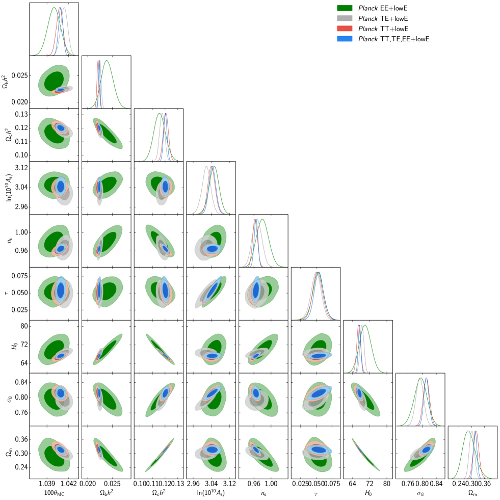
This pull is then mitigated in combination with temperature due to the larger uncertainty in the determination by TE,EE only. Similar considerations hold for the alternative CamSpec high- likelihood, which leads to a 68 % CL result , consistent with the baseline Plik reported in Eq. (10). Overall, the cosmological parameters from Planck baseline temperature, polarization, and temperature-polarization cross-correlation separately and combined are very consistent, as can be seen from Table 2 and Fig. 2 for the CDM model.
After combining with Planck lensing, we obtain
| (12) | ||||
| (13) |
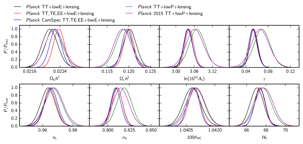
The shift in (and, more generally, in the cosmological parameters of the base-CDM model) obtained when Planck lensing is combined with TT,TE,EE+lowE is smaller than in 2015 because of the improved polarization likelihoods. The combination with lensing is, however, powerful for breaking parameter degeneracies in extended cosmological models, and, therefore, for this 2018 release we will consider the full information contained in temperature, polarization, and lensing, i.e., TT,TE,EE+lowE+lensing, as the baseline Planck data set. Figure 3 shows a comparison of the Planck 2018 baseline results with those from alternative likelihoods and from the 2015 baseline for the CDM cosmological parameters.
As in 2013 and 2015, BAO measurements from galaxy surveys are consistent with Planck. When BAO data are combined, we obtain for the base-CDM cosmology:
| (14) | ||||
The combination with BAO data decreases (increases) the marginalized value of () obtained by Planck, and this effect is compensated for by a shift in towards slightly larger values.
3.2 Ruling out
One of the main findings drawn from previous Planck releases was that the scale-independent Harrison-Zeldovich (HZ) spectrum (Harrison 1970; Zeldovich 1972; Peebles & Yu 1970) is decisively ruled out. This conclusion is reinforced in this release: in standard CDM late-time cosmology, the scalar spectral index from Table 2 lies , , and away from , for Planck TT+lowE, Planck TT,TE,EE+lowE, and Planck TT,TE,EE+lowE+lensing, respectively. The corresponding effective between the power-law spectrum and the best-fit HZ model are , , and .
Simple one-parameter modifications of the cosmological model are not sufficient to reconcile a scale-invariant power spectrum with Planck data. For instance, when the effective number of neutrino species is allowed to float for a cosmology with a scale-invariant spectrum, the effective with respect to the power-law spectrum are , , and , respectively.
When instead the assumption of flat spatial sections is relaxed,777For non-flat models the power spectra encode the eigenvalues of the corresponding Laplacian operator of the spatial sections and scale invariance holds at scales much smaller than the curvature radius. we obtain effective values of , , and , respectively, for the same data sets. Therefore, the corresponding closed cosmological models fitting Planck TT+lowE (, km s-1 Mpc-1 at 68 % CL), Planck TT,TE,EE+lowE (, km s-1 Mpc-1 at 68 % CL), and Planck TT,TE,EE+lowE+lensing (, km s-1 Mpc-1 at 68 % CL) provide a worse fit compared to the tilted flat CDM model.888This is not a new result based on the Planck 2018 release, but just an update of a similar conclusion also reached with the Planck 2015 data. Compared to the flat CDM tilted model, we obtain , , and with Planck 2015 TT+lowP, Planck 2015 TT,TE,EE+ lowP, and Planck 2015 TT,TE,EE+lowP+lensing, respectively. Therefore, even with Planck 2015 data, a closed model with provides a worse fit than tilted CDM and is not compelling as claimed in Ooba et al. (2017).
3.3 Constraints on the scale dependence of the scalar spectral index
The Planck 2018 data are consistent with a vanishing running of the scalar spectral index. Using Planck TT,TE,EE+lowE+lensing we obtain
| (15) |
These results are consistent with, and improve on, the Planck 2015 result, (PCP15).
As discussed in PCI13 and PCI15, a better fit to the temperature low- deficit was found in 2015, thanks to a combination of non-negative values for the running and the running of the running. The Planck 2018 release has significantly reduced the parameter volume of this extension of the base-CDM model. The Planck 2018 TT(TT,TE,EE)+lowE+lensing constraints for the model including running of running are
| (16) | ||||
| (17) | ||||
| (18) |
all at 68 % CL. It is interesting to note that the high- temperature data still allow a sizable value for the running of the running, although slightly decreased with respect to the Planck 2015 results (PCI15). However, when high- Planck 2018 polarization data are also included, and are tightly constrained.
The model including a scale-dependent running can produce a better fit to the low- deficit at the cost of an increase of power at small scales; this latter effect is constrained in this release. As an example of a model with suppression only on large scales, we also reconsider the phenomenological model with an exponential cutoff:
| (19) |
which can be motivated by a short stage of inflation (Contaldi et al. 2003; Cline et al. 2003) (see also Kuhnel & Schwarz (2010), Hazra et al. (2014a), and Gruppuso et al. (2016) for other types of large-scale suppressions). We do not find any statistically significant detection of using either logarithmic or linear priors and for different values of , with any combination of Planck baseline likelihoods. We have also checked that these results depend only weakly on the exclusion of the quadrupole in SimAll and are stable to the substitution of Commander and SimAll with the joint temperature-polarization likelihood based on the 70-GHz channel.
3.4 Constraints on spatial curvature
| Cosmological model | Parameter | Planck TT,TE,EE | Planck TT,TE,EE | Planck TT,TE,EE |
| CDM+ | +lowEB+lensing | +lowE+lensing+BK15 | +lowE+lensing+BK15+BAO | |
| + | ||||
| + | ||||
| + | ||||
| [eV] | ||||
| + | ||||
| + | ||||
Since the vast majority of inflation models predict that the Universe has been driven towards spatial flatness, constraints on the spatial curvature provide an important test of the standard scenario. Therefore in this subsection we extend the base-CDM model with the addition of the spatial curvature parameter, . For the case of Planck TT,TE,EE+lowE+lensing, we find a constraint of
| (20) |
The inclusion of Planck lensing information only weakly breaks the geometrical degeneracy (Efstathiou & Bond 1999) which results in the same primary fluctuations while varying the total matter density parameter, , and . The degeneracy can be effectively broken with the addition of BAO data, in which case Planck TT,TE,EE+lowE+lensing+BAO gives
| (21) |
Although is one of the cosmological parameters exhibiting some differences between Plik and Camspec, the constraints in Eqs. (20) and (21) are quite robust due to the inclusion of lensing (and BAO) information.
A constraint on the curvature parameter can be translated into a constraint on the radius of curvature, , via
| (22) |
in units such that . For the case of Planck TT,TE,EE+lowE+lensing+BAO we find
| (23) | ||||
| (24) |
both at confidence. These lengths are considerably greater than our current (post-inflation) particle horizon, at Gpc.
Our tightest constraint, Eq. (21), tells us that our observations are consistent with spatial flatness, with a precision of about 0.4 %. However, even if inflation has driven the background curvature extremely close to zero, the presence of fluctuations implies a fundamental “cosmic variance” for measurements of curvature confined to our observable volume. In particular, the known amplitude of fluctuations implies a standard deviation for of roughly (Waterhouse & Zibin 2008). Therefore our best constraint is still a factor of roughly above the cosmic variance limit for a flat universe. A future measurement of negative curvature above the cosmic variance floor would point to open inflation (Gott 1982; Gott & Statler 1984; Bucher et al. 1995; Yamamoto et al. 1995; Ratra & Peebles 1995; Lyth & Stewart 1990), while a measurement of positive curvature could pose a problem for the inflationary paradigm due to the difficulty of producing closed inflationary models (Kleban & Schillo 2012).
Alternatively, excess spatial curvature might be evidence for the intriguing possibility that there was “just enough” inflation to produce structure on the largest observable scales. Indeed an upper limit on spatial curvature implies a lower limit on the total number of -folds of inflation (see, e.g., Komatsu et al. 2009). We can relate these limits to the number of -folds of inflation, , after scale left the Hubble radius during inflation, to be given explicitly in Eq. (47). We define the (constant) curvature scale, , as the inverse of the comoving radius of curvature, i.e.,
| (25) |
In the absence of special initial conditions, inflation will begin with a curvature parameter of order unity. Equation (25) then implies that at the start of inflation, i.e., the curvature scale is “exiting the horizon” at that time. Then the lower limit on the number of -folds of inflation will simply be , i.e., the number of -folds after scale left the Hubble radius during inflation. With Eq. (47) this gives999This expression ignores a negligible correction, , due to the different inflationary potential scales at and exit.
| (26) |
With the pivot scale of Mpc-1 (for comparison with the values in Sect. 4.2) and our tightest upper limit on from Eq. (21), this becomes
| (27) |
That is, our constraint on spatial curvature implies that inflation must have lasted at least about 5 -folds longer than required to produce the pivot scale . Equation (27) provides a model-independent comparison between the -folds required to solve the flatness problem (to current precision) and to produce large-scale fluctuations (at scale ). We stress that this limit assumes a unity curvature parameter at the start of inflation (although the dependence on this assumption, being logarithmic, is weak).
For comparison with the result of Komatsu et al. (2009), we can simplify to the case of instantaneous thermalization and constant energy density during inflation. Then we find
| (28) |
where is the reheating temperature.
3.5 Constraints on the tensor-to-scalar ratio
This subsection updates constraints on the tensor-to-scalar ratio assuming that the tensor tilt satisfies the consistency relation, , which is the case for slow-roll inflation driven by a single scalar field with a canonical kinetic term.
By combining Planck temperature, low- polarization, and lensing we obtain
| (29) |
This constraint slightly improves on the corresponding Planck 2015 95 % CL bound, i.e., (PCI15), and is unchanged when high- polarization data are also combined. Note that by using CAMspec instead of Plik as the high- joint temperature-polarization likelihood, we obtain a slightly looser bound, i.e., at 95 % CL. By including the Planck -mode information at in the low- polarization likelihood, the 95 % CL constraint is essentially unchanged.
Since inflationary gravitational waves contribute to CMB temperature anisotropies mostly at , the low- temperature deficit contributes in a nontrivial way to the Planck bound on . By excising the temperature data, the constraint on with Planck TT,TE,EE+lensing+lowEB relaxes to
| (30) |
This result improves on the 2015 95 % CL result, i.e., (PCI15), because of the inclusion of high- polarization and of the improved determination of .
Since this Planck constraint on relies on temperature and -mode polarization, the Planck-only limit depends somewhat on the underlying cosmological model. Table 3 shows the constraints on and for a few important extensions of CDM plus tensors, which include a non-zero running, a non-zero spatial curvature, and a non-minimal neutrino sector. We observe that the bound on is relaxed by at most 30 % when the scale dependence of the scalar tilt is allowed to vary. In all the other extensions the Planck bound is modified at most by 10 %, demonstrating the constraining power of the Planck 2018 release in reducing the degeneracy of the tensor-to-scalar ratio with other cosmological parameters. As far as the scalar tilt is concerned, we find the largest shift (by roughly higher) when the assumption of spatial flatness is relaxed.
A -mode polarization measurement can further tighten the constraint on and help in reducing its degeneracies with other cosmological parameters that may appear when using only temperature and -mode polarization data. After the release of the first BICEP-Keck Array-Planck (BKP) joint cross-correlation, constraints on from -mode polarization data alone have become tighter than those based on Planck data alone, thanks to the inclusion of the 95-GHz channel (BK14) and of the 220-GHz channel (BK15). By combining the Planck 2018 and BK15 data we obtain
| (31) |
This bound improves on the corresponding one obtained in combination with BK14, i.e., at 95 % CL. Note that by using CAMspec instead of Plik as high- TT,TE,EE likelihood, we obtain a slightly looser bound, i.e., at 95 % CL. The effectiveness of the combination with the BK15 likelihood in constraining is also remarkable in the extensions of CDM plus tensors, as can be seen from Table 3. By further combining with BAO the limits for are only slightly modified.
The Planck 2018 baseline plus BK15 constraint on is equivalent to an upper bound on the energy scale of inflation when the pivot scale exits the Hubble radius of
| (32) |
Equivalently, this last result implies an upper bound on the Hubble parameter during inflation of
| (33) |
3.6 Beyond the tensor-to-scalar ratio consistency condition
The increasing constraining power of -mode polarization data allows us to set upper bounds on without imposing the consistency condition for the tensor tilt, , which is motivated by standard slow-roll single-scalar-field inflation. Deviations can occur in multifield inflation (Bartolo et al. 2001; Wands et al. 2002; Byrnes & Wands 2006), in the models with generalized Lagrangians (Garriga & Mukhanov 1999; Kobayashi et al. 2010), in gauge inflation (Maleknejad et al. 2013), or in a more radical way in alternative models to inflation (Gasperini & Veneziano 1993; Boyle et al. 2004; Brandenberger et al. 2007).
As the current data do not lead to a detection of a non-zero tensor amplitude, virtually any value of would give a good fit as long as is close enough to zero. Therefore, as in PCI15, we characterize the tensor perturbations by two well-constrained parameters that we choose to be at two different scales, (), with Mpc-1 and Mpc-1, and assume a power-law power spectrum. We call this two-parameter extension of the CDM model the “CDM+” model. We also quote our results in terms of , calculated from the primary parameters as and . For we choose Mpc-1, which corresponds roughly to the decorrelation scale of and when using the Planck and BK15 data.
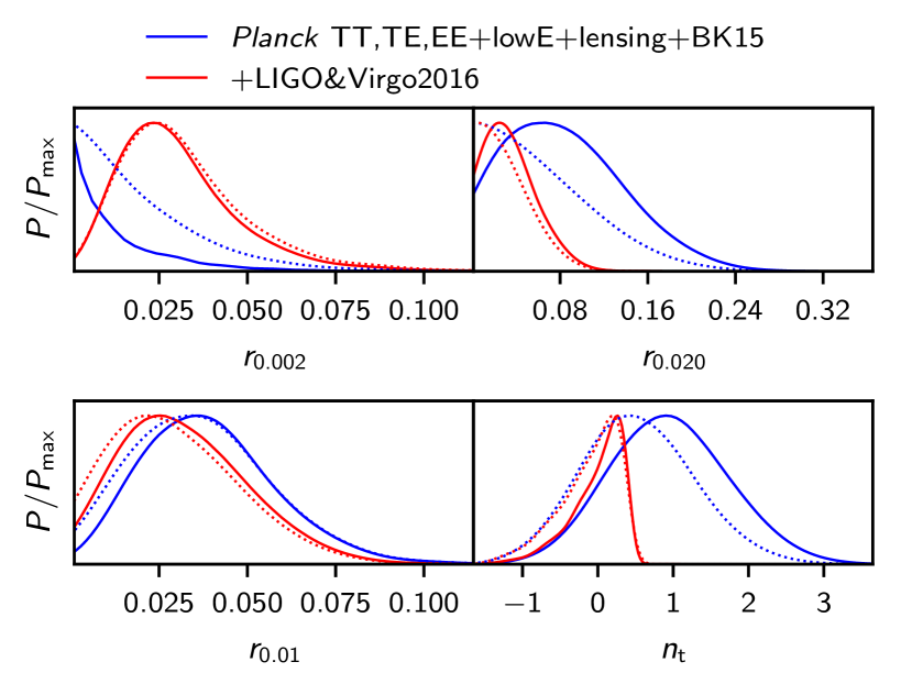
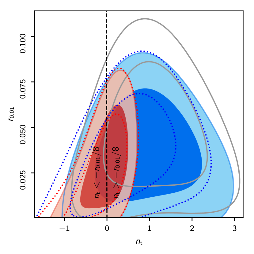
The one-dimensional posteriors are displayed in Fig. 4 (which also shows an additional data set, “LIGO&Virgo2016,” discussed at the end of this subsection). We obtain for the CDM+ model:
| (34) |
The constraints on the derived tensor parameters are and at 95 % CL.
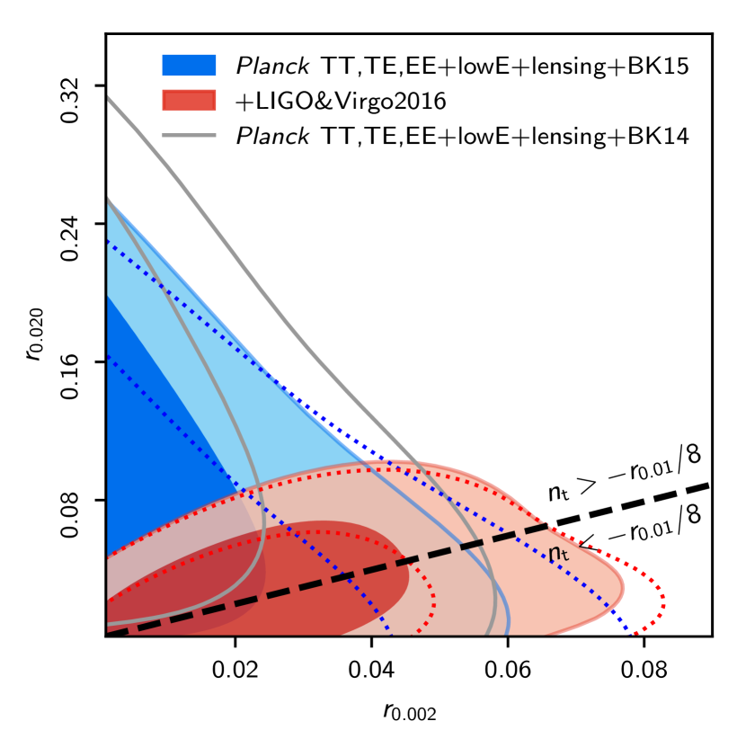
The left and right panels of Fig. 5 show the two-dimensional contours for the primary parameters and the derived ones , respectively. The consistency condition, , denoted by the dashed lines, is fully compatible with Planck+BK15 data. However, a very blue tensor tilt with and is still within the 68 % CL region. Indeed, despite the larger amplitude of the primordial tensor power spectrum at small scales for blue , the tensor modes are suppressed when re-entering the Hubble radius, which leads to damping of the observational signal at high . This explains why the 68 % CL CMB constraint on is about a factor of four weaker than the one on . Fig. 5 also shows a slight improvement of constraints by BK15 compared to the older BK14 data.
A stochastic background of gravitational waves (GWs) with a blue tensor tilt could be further constrained at much shorter wavelengths, such as those probed by ground-based interferometers dedicated to the direct detection of GWs. For example, assuming a scale-invariant tensor spectrum and using the frequency range (20–85.8) Hz, which corresponds to the wavenumbers –Mpc-1, LIGO and Virgo set an upper bound on the GW density parameter of at 95 % CL (Abbott et al. 2017). While these scales are likely to be dominated by astrophysical sources, such as GWs from binary mergers, we next examine what constraints the LIGO&Virgo upper bound sets on primordial tensor perturbations, if we assume that they had a power-law spectrum all the way from CMB scales to ultra-short scales. We refer the interested reader to Meerburg et al. (2015) and Cabass et al. (2016) for the use of alternative data on short scales or of additional constraints on the effective energy-momentum tensor of the stochastic background of GWs averaged over wavelengths.
We obtain a conservative upper limit on the primordial contribution by demanding that the GW density from our scale-dependent primordial tensor perturbations (Meerburg et al. 2015; Abbott et al. 2017; Cabass et al. 2016),
| (35) |
stays below the above-quoted limit at least at Mpc-1 (Hz). The posterior probability densities when this constraint is included in the analysis as a half-Gaussian prior are compared with those obtained by Planck+BK15 alone in Figs. 4 and 5. LIGO&Virgo sets a very high upper bound101010Using Eq. (35), the upper bound corresponds to a tensor perturbation amplitude , where we used . Assuming further for the scalar perturbations that and at , this can be converted into an upper bound at . on at ultra-high , separated from CMB scales by a factor of in . Due to the long arm length, this effectively provides a cutoff for and excludes the bluest spectra that were allowed by the CMB alone, leading to
| (36) |
or and . The consistency condition is also compatible with these tighter constraints, as can be seen by comparing the red contours and dashed black lines in Fig. 5. As LIGO&Virgo pushes down (and we assume a power-law tensor spectrum), the upper bound on becomes weaker than with the CMB alone. This is not surprising, since the system is analogous to a see-saw with a pivot point at Mpc-1, where the data are the most sensitive to the tensor perturbations (taking into account also the transfer function from primordial tensor perturbations to the observable -mode signal). Once one end of the see-saw is pushed down the other end can go up without disturbing the spectrum too much at the middle scales. We will observe analogous behaviour with isocurvature perturbations, for which we also assume a power-law spectrum and have only an upper bound (not a detection); see Sect. 9.3.
4 Implications for single-field slow-roll inflationary models
In this section we discuss the implications of the Planck 2018 likelihood for standard single-field slow-roll inflation. We first update the results for the Hubble flow functions (HFFs) and the potential slow-roll parameters obtained by the analytic perturbative expansion in terms of the HFFs for the primordial spectra of fluctuations. For definitions of the HFF hierarchy and the potential slow-roll parameters see Table 1. We then present a Bayesian comparison for a representative selection of standard slow-roll inflationary models.
4.1 Constraints on slow-roll parameters
Exploiting the approximate analytic expressions for the primordial power spectrum of scalar and tensor fluctuations obtained by the Green’s function method (Stewart & Lyth 1993; Gong & Stewart 2001; Leach et al. 2002), we can construct constraints on the slow-roll parameters.
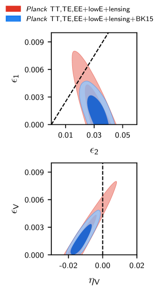
When restricting to parameters first order in the HFFs, we obtain with Planck TT,TE,EE+lowE+lensing(+BK15)
| (37) | |||||||
| (38) |
The Planck TT,TE,EE+lowE+lensing(+BK15) constraints on the slow-roll potential parameters and can be obtained by an exact remapping of the constraints on the HFF parameters (Leach et al. 2002; Finelli et al. 2010) given above:
| (39) | ||||||
| (40) |
As can be seen from Fig. 6, the 95 % CL allowed contours are in the region of concave potentials when BK15 is combined with Planck 2018 data.
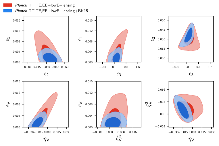
When contributions to the primordial power spectra that are second-order in the HFFs are included, for Planck TT,TE,EE+lowE+lensing(+BK15) we obtain the following constraints on the slow-roll HFFs:
| (41) | ||||||
| (42) | ||||||
| (43) |
and on the slow-roll potential parameters we obtain:
| (44) | ||||||
| (45) | ||||||
| (46) |
The marginalized 68 % and 95 % CLs for the slow-roll HFF and potential parameters, allowing , with Planck data alone or in combination with BK15, are displayed in Fig. 7.
4.2 Implications for selected slow-roll inflationary models
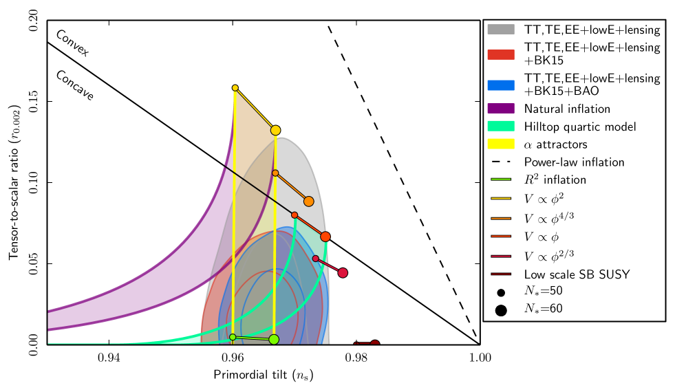
The predictions for to first order in the slow-roll approximation for a few inflationary models are shown in Fig. 8, which updates figure 12 of PCI15 and figure 1 of PCI13 with the same notation. These predictions are calculated for scale Mpc-1 and include an uncertainty in the number of -folds of .
|
In the following we discuss the implications of the Planck 2018 data release by taking into account the uncertainties in the entropy generation stage for a selection of representative standard single-field slow-roll inflationary models, updating the analysis reported in PCI13 and PCI15. As in PCI15, we use the primordial power spectra of cosmological fluctuations generated during slow-roll inflation parameterized by the HFFs, , to second order, which can be expressed in terms of the parameters of the inflationary model and the number of -folds to the end of inflation, (Liddle & Leach 2003; Martin & Ringeval 2010), given by (PCI13)
| (47) |
where is the energy density at the end of inflation, is the present Hubble scale, is the potential energy when left the Hubble radius during inflation, characterizes the effective equation of state between the end of inflation and the thermalization energy scale , and is the number of effective bosonic degrees of freedom at the energy scale . We fix and , and we use modified routines of the public code ASPIC111111http://cp3.irmp.ucl.ac.be/~ringeval/aspic.html (Martin et al. 2014b). In order to make contact with Fig. 8, we consider the pivot scale Mpc-1 in this subsection. We assume the uniform priors for the cosmological parameters listed in Table 4, and logarithmic priors on (over the interval ) and (over the interval ). Prior ranges for additional parameters in the inflationary models considered are listed in Table 5. In this paper we consider the implications of the Planck 2018 data for the selection of representative models studied in PCI15 by restricting ourselves to , when the potential can be approximated as during the coherent oscillation regime after inflation, or simply when the potential considered describes only the inflationary stage.121212Note that some inflationary potentials in this selection are a valid model for all stages, from the slow-roll phase all the way to coherent oscillations around the minimum during reheating, while others are “incomplete” in the sense that they only describe the slow-roll regime. The hilltop, D-brane, potential with exponential tails, and spontaneously broken SUSY models fall into the latter category and rely on additional terms, denoted by the ellipses, to complete the potential at the end of inflation. With the increasing precision of CMB data and accompanying accuracy requirements for theoretical predictions, the precise form of the additional terms may affect the scientific interpretation of some incomplete models, as pointed out for the case of quadratic hilltop and double-well inflationary models in PCI15. For data we use the full constraining power of Planck, i.e., Planck TT,TE,EE+lowE+lensing, in combination with BK15.
| Inflationary model | Potential | Parameter range | ||
|---|---|---|---|---|
| Power-law potential | ||||
| Power-law potential | ||||
| Power-law potential | ||||
| Power-law potential | ||||
| Power-law potential | ||||
| Power-law potential | ||||
| Non-minimal coupling | ||||
| Natural inflation | ||||
| Hilltop quadratic model | ||||
| Hilltop quartic model | ||||
| D-brane inflation () | ||||
| D-brane inflation () | ||||
| Potential with exponential tails | ||||
| Spontaneously broken SUSY | ||||
| E-model | ||||
| E-model | ||||
| T-model | ||||
| T-model |
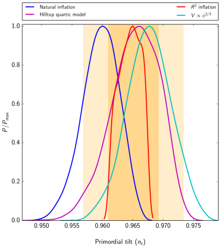
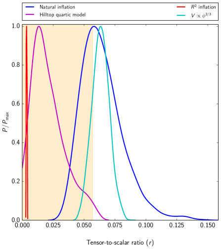
The and the Bayesian evidence values for a selection of inflationary models with respect to the model (Starobinsky 1980; Mukhanov & Chibisov 1981; Starobinsky 1983) are shown in Table 5. Figure 9 shows the resulting marginalized probability densities of and at Mpc-1 for a few inflationary models with the above specified priors, compared to the corresponding 68 % and 95 % CL limits obtained from a CDM-plus-tensor fit. We refer the interested reader to PCI15 for a concise description of the inflationary models studied here and we limit ourselves here to a summary of the main results of this analysis.
-
•
The inflationary predictions (Mukhanov & Chibisov 1981; Starobinsky 1983) originally computed for the model (Starobinsky 1980) to lowest order,
(48) are in good agreement with Planck 2018 data, confirming the previous 2013 and 2015 results. The 95 % CL allowed range is compatible with the basic predictions , corresponding to GeV (Bezrukov & Gorbunov 2012). A higher reheating temperature GeV, as predicted in Higgs inflation (Bezrukov & Shaposhnikov 2008), is also compatible with the Planck data.
-
•
Monomial potentials (Linde 1983) with are strongly disfavoured with respect to the model. For these values the Bayesian evidence is worse than in 2015 because of the smaller level of tensor modes allowed by BK15. Models with or (Silverstein & Westphal 2008; McAllister et al. 2010, 2014) are more compatible with the data.
-
•
There are several mechanisms which could lower the predictions for the tensor-to-scalar ratio for a given potential in single-field inflationary models. Important examples are a subluminal inflaton speed of sound due to a non-standard kinetic term (Garriga & Mukhanov 1999), a non-minimal coupling to gravity (Spokoiny 1984; Lucchin et al. 1986; Salopek et al. 1989; Fakir & Unruh 1990), or an additional damping term for the inflaton due to dissipation in other degrees of freedom, as in warm inflation (Berera 1995; Bastero-Gil et al. 2016). In the following we report on the constraints for a non-minimal coupling to gravity of the type , with , and a quartic potential. For this model we compute the theoretical predictions in terms of HFFs and number of -folds to the end of inflation in the Einstein frame as for the model above, but we omit the technical details for the sake of brevity.131313In this model the potential in the Einstein frame is known only in implicit form (see, for instance, Garcia-Bellido et al. (2009)) and the algebra is therefore more complicated. Our results show that a quartic potential, which would be excluded at high statistical significance for a minimally-coupled scalar inflaton as seen from Table 5, can be reconciled with the Planck and BK15 data for : we obtain a 95 % CL lower limit with .
- •
-
•
Within the class of hilltop inflationary models (Boubekeur & Lyth 2005) we find that a quartic potential provides a better fit than a quadratic one. In the quartic case we find the 95 % CL lower limit .
- •
- •
-
•
Planck 2018 and BK15 data strongly disfavour the hybrid model driven by logarithmic quantum corrections in spontaneously broken supersymmetric (SB SUSY) theories (Dvali et al. 1994), with .
-
•
Planck and BK15 data set tight constraints on attractors (Kallosh et al. 2013; Ferrara et al. 2013). We obtain and at 95 % CL for the E-model. We obtain slightly tighter 95 % CL bounds for the T-model, i.e., and . Given the relation between the curvature of the Kähler geometry and in some of the T-models motivated by supergravity, Planck and BK15 data imply a lower bound on , which is still in the low-curvature regime. The discrete set of values with an integer in the range motivated by maximal supersymmetry (Ferrara & Kallosh 2016; Kallosh et al. 2017) is compatible with the current data.
5 Reconstruction of the inflaton potential
5.1 Taylor expansion of in the observable region
In this section, as in section 6 of PCI13 and section 7.1 of PCI15, we try to reconstruct the inflaton potential only in its observable window, making no assumptions about the end of inflation. The motivation for being so conservative is that what happens after the inflaton rolls down beyond this range might not be captured by the simplest descriptions. More elaborate treatments would be required, for instance, in the case of a non-trivial potential shape before the end of inflation, a waterfall transition involving extra scalar fields, or several short inflationary stages between the time at which CMB scales exit the Hubble radius and the nucleosynthesis epoch. The analysis of this section relies, however, on the assumption that the potential is smooth enough inside the observable window to be described by a Taylor expansion up to order four. Note that this assumption is much weaker than assuming that a Taylor expansion is valid up to the end of inflation. However, it excludes from the analysis potentials with sharp features in the observable window, such as those studied in the next sections.
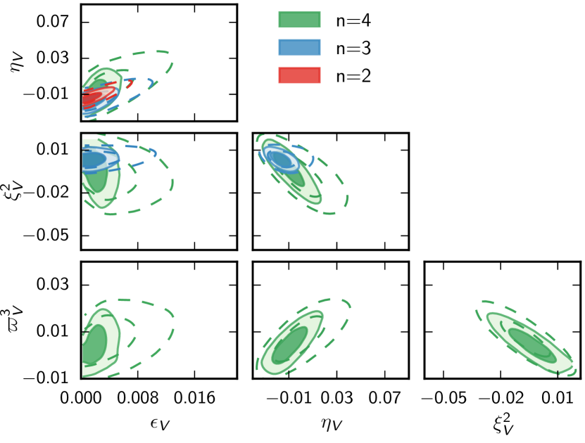
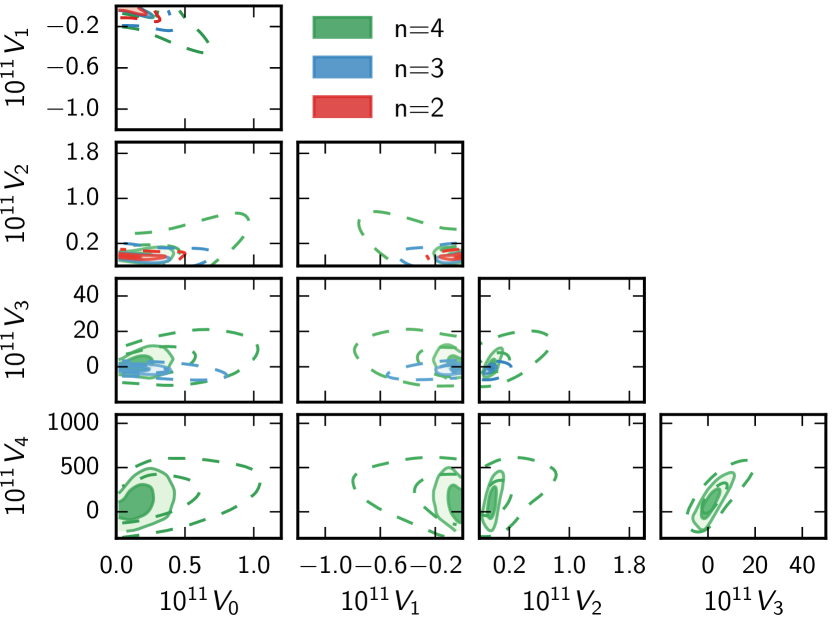
We perform the Taylor expansion around the value of the inflaton field evaluated precisely at the time when the pivot scale fulfills the relation . We separately study the cases where the expansion is performed at order , , or . We compute the primordial spectrum with a full integration of the Fourier mode evolution, using the inflationary module of the CLASS code. Although this method assumes no slow-roll approximation at any point, we speed up the convergence of the Markov Chain by taking flat priors not directly on the five Taylor coefficients , but on combinations of them matching the definitions of the potential slow-roll parameters presented in table 2 of PCI13. Even beyond the slow-roll approximation, these combinations provide nearly linear contributions to the tilt, running, running of the running, etc., of the scalar and tensor spectrum. Hence, they are directly related to observable quantities and well constrained by the data. Instead, if we ran with flat priors on , the convergence would be plagued by complicated parameter degeneracies.
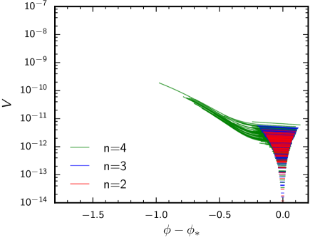
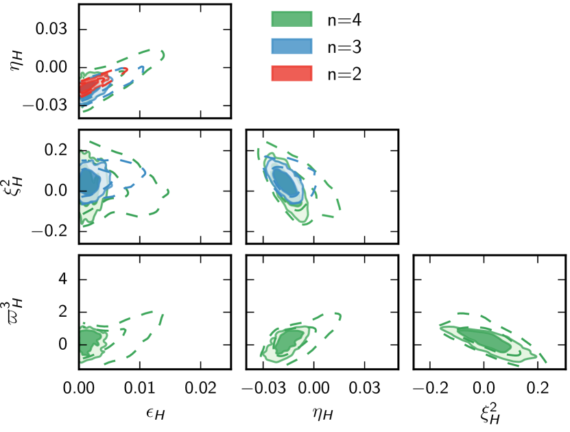
The results of this analysis are shown in the panels of Fig. 10 and Table 6 for , , and , using two data sets for each: Planck TT,TE,EE+lowE alone; or Planck TT,TE,EE+lowE+lensing+BK15. The plot in Fig. 10 deliberately has a lot of white space because, for the sake of comparison, we plotted it over the same parameter ranges as the same plot in PCI15. We notice some significant improvement. Comparing Planck TT,TE,EE+lowE results from 2015 and 2018, we find that error bars on individual parameters have typically been reduced by 30 % thanks to improved polarization data. Including BK data provides further constraining power. Comparing Planck 2015 TT+lowP+BAO and Planck 2018 TT,TE,EE+lowE+lensing+BK15, we find that the error bars on shrink by factors of 2 to 4. The new data tend to resolve degeneracies which previously appeared in the case and could be understood as a compensation mechanism between potentials with large running of the tilt, running of the running, tensor contribution, etc. The parameters and are perfectly compatible with zero (see Fig. 10 and Table 6), and so are and (see the contours on the parameters in Fig. 11). This is consistent with the fact that the new data set brings no evidence for running or running of the running. It also explains why the results of this section are close to those of Sect. 4.1, obtained under the slow-roll approximation. Similar to 2015, the best-fit value of running for is negative, but has moved down from to , and remains compatible with zero at the 1.0 level. For , the trend observed in 2015 to fit the data slightly better with a non-zero tensor contribution has disappeared. The decrease of the minimum effective when moving from to is insignificant and even smaller than in 2015, showing that the data do not require anything more complicated than an approximately parabolic shape for the inflaton potential within the observable window.
This can be checked by considering the random sample of well-fitting potentials presented in Fig. 12. Actually, for , a few of the plotted potentials have a non-parabolic “spoon-like” shape (with a kink and a plateau), because non-negligible values of are still allowed. However, this sub-class of models is by no means preferred over simpler parabolic-like potentials with a negligible ; otherwise, we would have obtained a better for . Hence one should not take from Fig. 12 the message that special potentials with a kink and a plateau are favoured by the Planck data. Comparing this plot to figure 15 of PCI15, we see that the models with the largest amplitude are excluded by stronger bounds on the tensor modes.
Finally, it is interesting to notice that the predictions for the parameters of the minimal CDM model, such as or , remain extremely stable when increasing the freedom in the inflaton potential.
| 2 | 3 | 4 | |
5.2 Taylor expansion of in the observable region
To assess the robustness of our method, in this section we repeat the analysis with a Taylor expansion of the Hubble function in the observable window, as we did in 2015. We refer the reader to section 7.2 of PCI15 for a precise description of this analysis, and we recall that the difference with respect to the reconstruction is more than a mere change of priors. For each value of , the new parameterization covers a slightly different range of potentials, and, more importantly, it naturally includes a marginalization over the uncertainty in the initial value of the derivative when the inflaton enters the observable window. Instead, in the previous analysis, was assumed to have reached the inflaton attractor solution, i.e., there was an implicit assumption that inflation started well before that time. In the analysis based on , inflation models with a minimal duration are not excluded by the priors.
The improvement with respect to the 2015 results is even more impressive in this case. Bounds on the parameters are typically 3 to 4 times stronger compared with 2015, as can be checked from Table 7 and Fig. 13. We found that a factor of 2 improvement comes from switching to the new set of low- likelihoods, and another factor of 2 from adding the BK likelihood. On the other hand, the use of more recent high- and lensing likelihoods has a modest impact.
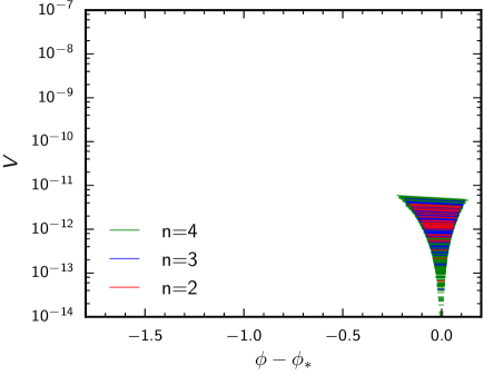
A consequence of these improved constraints can be seen in Fig. 14, when we compare it to its counterpart from 2015 (figure 20 in PCI15). Again, for a better comparison Fig. 14 uses the same scale as figure 20 of PCI15. For , the previously best-fitting models included many scenarios starting with a fast-roll stage, producing a tail with large before pivot-scale crossing. These models are now excluded by better polarization data and tensor constraints.
Going beyond the parabolic approximation for does not improve the goodness-of-fit: as in the potential-based analysis of Sect. 5.1, the s between , , and are negligible, and the parameters and related to and are compatible with zero.
| 2 | 3 | 4 | |
5.3 Taylor expansion of full
We now present a new analysis with less conservative assumptions than in the previous subsections. We switch to the hypothesis that the inflaton potential is very smooth not only within its observable window, but also until the end of inflation, such that its whole shape can be captured by a Taylor expansion. We further assume that inflation ends when the first slow-roll condition is violated (), without invoking any other field. Finally, we fix the number of -folds between Hubble crossing of the pivot scale and the end of inflation to , which implicitly relies on the hypothesis that no further inflationary stage took place at a later epoch.
Technically, the analysis pipeline for this case is similar to that of Sect. 5.1, except for an extra step in which the CLASS inflationary module integrates the background equations until the end of inflation, goes backwards in time by 55 -folds, and imposes that the Hubble crossing for the pivot scale matches that time.
These models are much more constrained than those of Sects. 5.1 and 5.2, since the -fold condition is imposed in addition to having a potential with a good shape within the observable window. The constraining power is then sufficient for running the MCMC chains directly with flat priors on .
Our results are presented in Figs. 15 and 16 and in Table 8. For models with a purely quadratic potential, the numerically computed tilt and tensor-to-scalar ratio depend almost exclusively on , thus they remain fixed to and . Such a large is in tension with the Planck data, and even more so with the Planck+BK data. Thus the effective is poor in the case and improves considerably when adding some freedom in going to . Indeed, the presence of an additional cubic term allows us to reach smaller values of the tensor-to-scalar ratio for roughly the same scalar tilt, and lowers by more than 13. Instead, when also adding a quartic term, we find no significant improvement in the goodness of fit, and the coefficient of the term is consistent with zero.
These findings are consistent with the global picture that Planck data prefer potentials which are concave in the observable window. The blue and green curves in the lower left panel of Fig. 16 illustrate the preference of the Planck+lensing+BK15 data for potentials with an inflection point, appearing qualitatively similar to scalar field potentials associated with spontaneous symmetry breaking models, hilltop models, new inflation, natural inflation, etc.
In these runs, the value of the scalar tilt running is always very precisely constrained around a value of . This does not come as a surprise if we keep in mind that these bounds are not imposed directly by the data, but rather by the class of inflationary potentials considered here, with potential parameters fixed by observational bounds on the amplitude and tilt of the scalar and tensor spectra. In other words, the running is not directly measured, but rather predicted as a function of the scalar/tensor amplitudes and scalar tilt. Interestingly, if combinations of future CMB and large-scale structure data with a wide lever arm in wavenumber space could become directly sensitive to such tiny values (which would require a factor of around 10 improvement in sensitivity compared to current CMB+BAO data), a very large class of currently successful inflationary models could be either confirmed or ruled out.
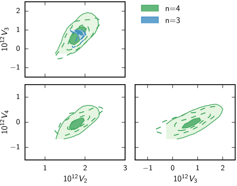
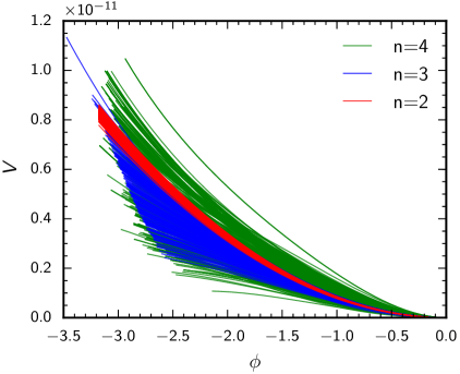
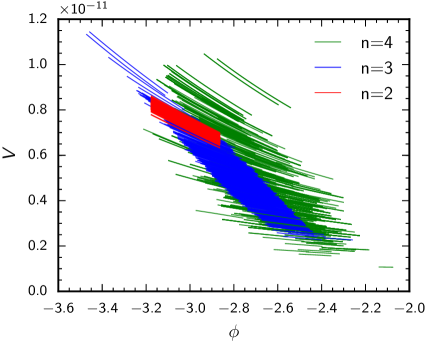
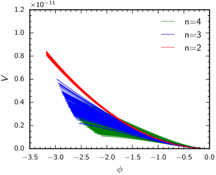
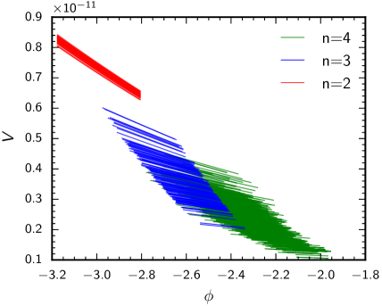
| 2 | 3 | 4 | |
5.4 Free-form potential reconstruction
As a complementary analysis to the previous three subsections, we next perform a free-form reconstruction of the inflationary potential with cubic splines, in a manner akin to the reconstructions of PCI15 and Sect. 6.2.1. Further plots and theoretical detail can be found in Handley et al. (2019).
A free-form reconstruction usually proceeds by parameterizing the function of interest via a spline and taking the locations of the interpolation knots as free parameters in a posterior distribution. These are then varied along with any other model parameters, and then marginalized out to yield a model-independent reconstruction of the function of interest. The analysis is run for differing numbers of knots, , and the Bayesian evidence is computed to allow for model comparison to determine how many knots are appropriate from the perspective of the data.
To reconstruct the inflationary potential , one cannot take a linear interpolating spline (as in Sect. 6.2.1), since the equations of motion in general depend on first (and sometimes second) derivatives of . We therefore choose to parameterize the second derivative of the log-potential as a linear spline. The log-potential is computed by integrating this function twice, yielding a function with two additional free parameters—a global offset and a gradient. Our reconstruction function is therefore
| (49) | ||||
| (50) | ||||
| (53) |
Here is a standard linear spline dependent on knots, is the potential at the pivot scale, and is the gradient of the log-potential at the pivot scale.
In general, any reconstruction of the potential will be sensitive only to the observable window of inflation in , where and are defined as the field values when the largest and smallest observable scales and exit the Hubble radius during inflation. Regions of the potential outside these values are unconstrained by current CMB data. In our analysis, we take and , which encompasses the multipole range constrained by Planck (see Sect. 6.2.1). The locations of the reconstruction knots should be distributed throughout this observable window. Whilst the locations and heights themselves influence the size of the observable window, a reasonable approach is to first estimate it using the unperturbed potential (i.e., setting ). This gives an alternative range . The priors on all our variables are indicated in Table 9.
| Parameters | Prior type | Prior range |
|---|---|---|
| Discrete uniform | ||
| Uniform | ||
| Log-uniform | ||
| Uniform | ||
| Sorted uniform | ||
| Indirect constraint |
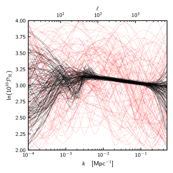
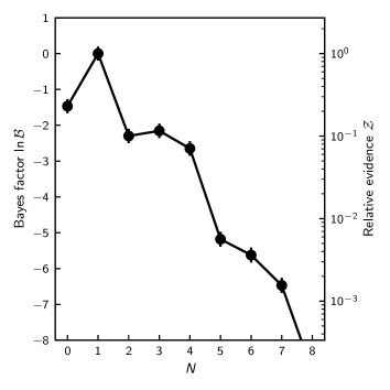
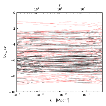
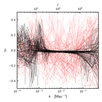
Our results are detailed in Fig. 17. The Bayesian evidence shows that the reconstruction preferred by the data is that using , corresponding to a constant non-zero . This indicates that the Planck data do not significantly constrain the inflationary potential within the window any further than up to a quadratic term in a Taylor expansion. It is illuminating, however, to consider adding further structure to the potential, and Fig. 17 shows reconstructions for .
Considering the predictive posterior of the primordial power spectrum, we see that our parameterization is sufficient to exhibit the deficit at , cosmic variance at low , and the loss of resolution at high , as seen in Sect. 6.2.1. Consistent with the rest of the analyses, is unconstrained, whilst the Planck data provide relatively powerful constraints on within the observable window of inflation.
6 Primordial power spectrum reconstruction
This section reports results for the non-parametric reconstruction of the primordial scalar power spectrum using the new Planck 2018 likelihoods, as well as comparisons with the previously reported results for the Planck 2013 and 2015 releases. The objective here is to search for deviations from a simple power-law primordial power spectrum (i.e., ) in a manner that does not presuppose any particular theoretical model giving rise to such deviations. This work is complementary to the searches considered in Sect. 7, where particular functional forms for such deviations motivated by theory are investigated.
Here we apply three distinct nonparametric methods. In 2013 only the first method was used to reconstruct the primordial power spectrum, the so-called “penalized likelihood” method, for which the 2018 results are presented in Sect. 6.1. In 2015 two additional methods were also used: a linear spline method (discussed in Sect. 6.2) for which both the number of knots and their positions were allowed to vary, and ideas from Bayesian model selection were applied to determine the appropriate number of knots; and a method using cubic splines (discussed in Sect. 6.3). Although the discussion below includes some description of each method in order to make the paper self-contained, for details the reader is referred to the 2013 and 2015 papers. Here we specify only those details specific to the 2018 analysis or different from the choices in the 2013 and 2015 analyses. See references in PCI13 and Hunt & Sarkar (2014), Hazra et al. (2014b), and Hunt & Sarkar (2015) for other approaches to non-parametric reconstruction of the primordial power spectrum.
6.1 Penalized likelihood
The underlying idea of the penalized likelihood approach is to add a term to the log-likelihood that penalizes deviations from a perfect power-law spectrum. We parameterize the power spectrum as
| (54) |
where , and add the following term to :
| (55) |
where The interval is chosen to cover the range over which the likelihood is able to constrain the data. The two terms serve to pin the reconstruction to the simple power law where the data have almost no constraining power. One may imagine that should be infinite, but for numerical reasons a large but finite value is used to simplify the numerics. Numerically, for each the dimension of is chosen to be so large that the continuum version of the penalty given in Eq. (55) has been accurately approximated. For more details see Gauthier & Bucher (2012) and the extensive references therein to prior literature, as well as PCI13 and PCI15.
In Fig. 18 we show the results using Planck TT+lowE and in Fig. 19 we show the results for Planck TT,TE,EE+lowE. In both cases we have assumed the usual base-CDM model specified in PCP18, except that the power spectrum is now parameterized by a set of spline points. In addition to these spline points, we also maximize the likelihood with respect to the dimensionless Hubble parameter, , and the baryon, , and CDM, , densities. All other cosmological and nuisance parameters are the same as those quoted in PCP18.
For the TT-only case, the maximum deviations are , , , and for , , , and , respectively, for which the probabilities to exceed are 13 %, 28 %, 31 %, and 23 % (where we have taken into account the look-elsewhere effect). Similarly, for the TT,TE,EE case, the maximum deviations are , , , and for , , , and , respectively, for which the probabilities to exceed are 29 %, 23 %, 32 %, and 25 %. We consequently find no statistically significant evidence for a deviation from the simple power-law hypothesis. This result is consistent with the results previously reported for the Planck 2013 and 2015 releases using essentially the same method. It is likewise consistent with the results below in Sects. 6.2 and 6.3, which use different methods.
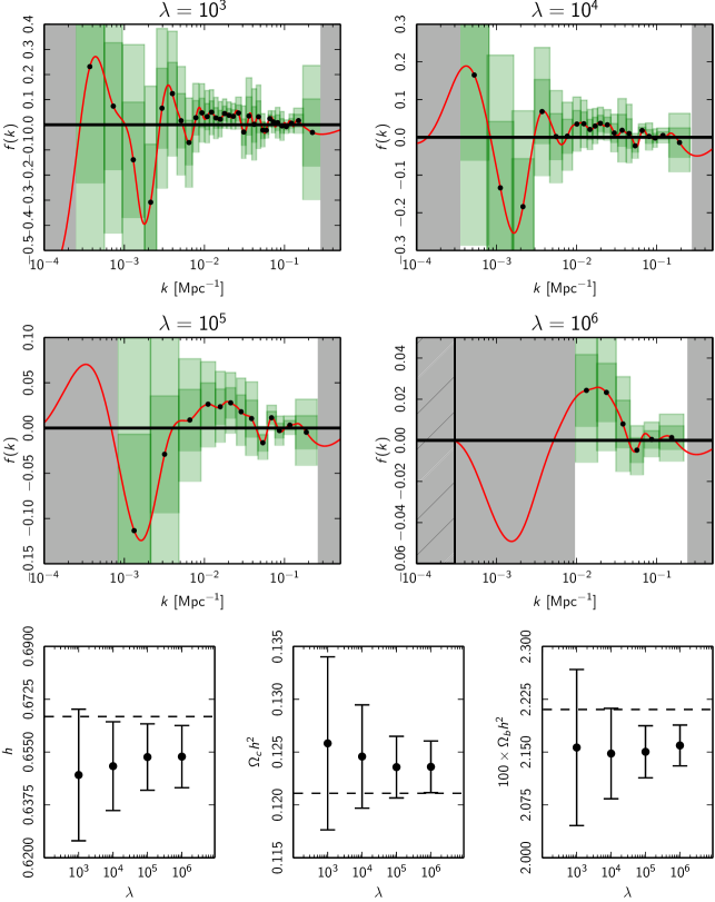
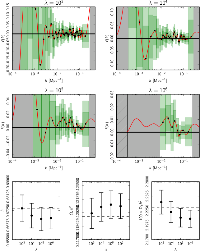
6.2 Bayesian reconstruction
To reconstruct the primordial power spectrum of curvature perturbations, we follow the methodology of section 8.2 of PCI15, using an -point interpolating logarithmic spline with the positions of the knots considered as free parameters in the full posterior distribution. The positions of the points in the plane are treated as likelihood parameters with log-uniform priors. Further, the -positions are sorted a priori such that , with and fixed. We compute posteriors and evidence values (conditioned on ) using PolyChord (Handley et al. 2015a, b), also varying all cosmological and nuisance parameters. We then use evidence values for each model to correctly marginalize out the number of knots .
To plot our reconstructions of , we compute the marginalized posterior distribution of conditioned on . The iso-probability confidence intervals are then plotted in the plane (see, e.g., Fig. 20), using code recorded in Handley (2018). To quantify the constraining power of a given experiment, we use the conditional Kullback-Leibler (KL) divergence as exemplified by Hee et al. (2016). For two distributions and , the KL divergence is defined as
| (56) |
and may be interpreted as the information gain in moving from a prior to a posterior (Raveri et al. 2016). For our reconstructions, we compute the KL divergence of each distribution conditioned on and , and then marginalize over using evidence values to produce a -dependent number which quantifies the compression or information that each data set provides at each value of . Further plots and theoretical detail can be found in Handley et al. (2019).
6.2.1 Update on Planck 2015
In PCI15, our analysis focussed predominantly on the TT+lowTEB data set. Here we present results for TT,TE,EE+lowE+lensing. First, in updating to the lowE likelihood, we find that there is a marked tightening in the constraint on the amplitude of the reconstructed spectrum at all values of . The improvement in the constraint can be seen directly in the predictive posterior plots (Fig. 20, top-left panel, and Fig. 21), and is quantified in Fig. 20 (bottom-right) via the KL divergence. The reason for the high- constraint provided by a low- likelihood change is due to the reduced uncertainty on that SimAll EE provides. This can be seen by examining the shifts in the underlying cosmological parameters in Fig. 2.
Upon adding TE and EE data, we find that the hint of a feature at is still present, in spite of the additional constraining power provided by polarization. Using polarization data, the case is now the most strongly favoured model by the evidence criterion. This indicates that there is some scope for models which account for low- cosmic variance to be preferred in a Bayesian sense. The other underlying cosmological parameters are unaffected by the additional degrees of freedom in the primordial power spectrum provided by the reconstruction.
In order to combine Planck polarization data with BK15, we also allow the tensor-to-scalar ratio to vary, and fix the tensor tilt via the inflationary consistency condition. As can be seen in the bottom-left panel of Fig. 20, upon adding BK15, the effect of the low- deficit is softened, but with otherwise little change to the reconstruction. We repeated our analysis with CamSpec in place of Plik and found our results to be qualitatively and quantitatively unchanged.
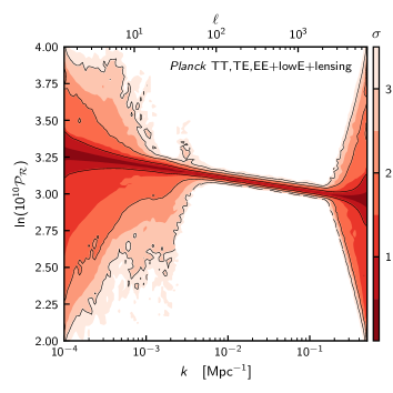
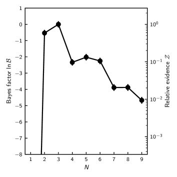
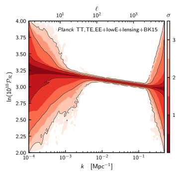
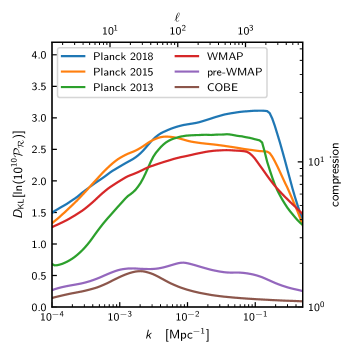
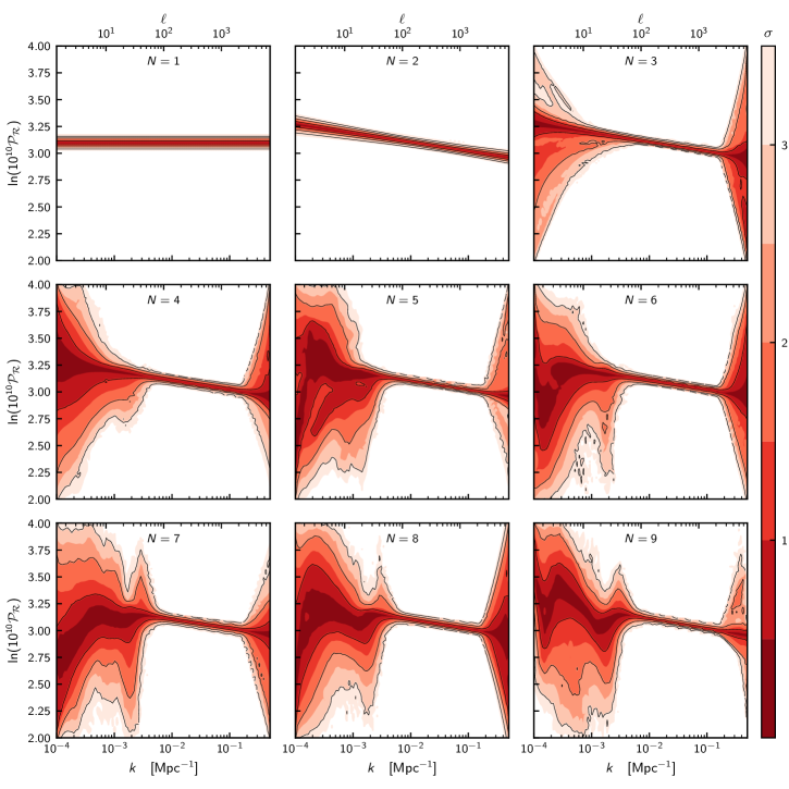
6.2.2 Free-form search for features
Next we examine the effect that sharp features in the primordial power spectrum can have on cosmological parameters. We model sharp features in the spectrum as a variable number of top-hat functions with varying widths, heights, and locations. On top of the traditional parameterization of the power spectrum, we place sharp top-hat features into the spectrum at locations with widths and heights (). That is, we set
| (57) |
where the square brackets in the summation denote a logical truth function as introduced by Graham et al. (1994). For values of , we treat the variables in parameterization (57) as parameters in a posterior distribution along with the traditional cosmological and Planck nuisance parameters, with priors as detailed in Table 10. We run with both linear and logarithmic priors on the -locations of the features, as this alters the sensitivity to the type of features uncovered. We sample the posteriors using PolyChord (Handley et al. 2015a, b).
| Parameter | Prior | Range |
|---|---|---|
| Sorted uniform | ||
| Uniform | ||
| Sorted log-uniform | ||
| Log-uniform | ||
| Uniform | ||
| Uniform | ||
| Uniform |
Figures 22 and 23 show our results. With the linear priors case, there are statistically insignificant features corresponding to the peaks of the spectrum, which arise due to the enhanced cosmic variance at these locations. With the logarithmic priors case, a stronger but still statistically insignificant feature is detected at , with a small deficit and surrounding enhancement of power. This case reproduces the results found in Sect. 6.2.1. In both cases, the Bayesian evidence shows preference for a no-features spectrum, and steadily declines as more features are added. The cosmological parameters remain unperturbed despite the introduction of features.
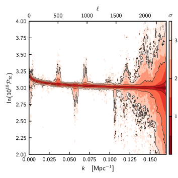
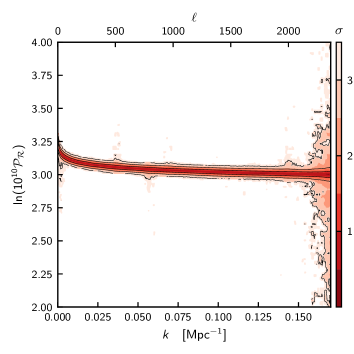
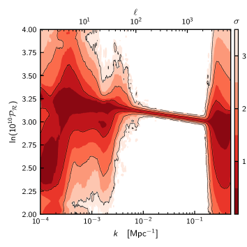
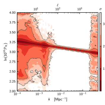
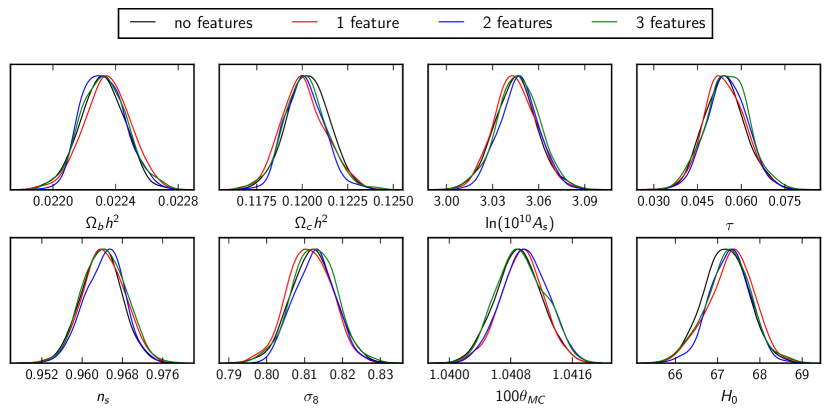
6.3 Cubic spline reconstruction
In this subsection we update the third method of reconstruction used in PCI15, in which was expanded in cubic splines localized in about uniformly spaced “knots,” , whose range was chosen to cover all relevant cosmological scales, from Mpc-1 to Mpc We single out the standard scalar power spectrum pivot scale as a “pivot knot” , with Its associated power is assigned a uniformly distributed prior. A tilted primordial power spectrum , with fixed spectral index is used as the fiducial baseline from which deviations are measured, expressed in terms of relative spectral shape parameters: for . For the results presented here, was chosen. As in PCI15 we continue to use cubic splines for the -space modes we expand in, with natural boundary conditions (i.e., vanishing second derivatives at the first and last knots). The treatment here is therefore quite analogous to that in Sect. 5.4, where the inflaton potential rather than the curvature power spectrum is expanded in cubic splines. Knot numbers up to 18 were reported in PCI15, and it was shown that 12 were sufficient to capture the variations desired by the Planck CMB data. The mode functions were also varied. For example, linear interpolation leads to similar reconstructions as long as enough knots are used. A weak uniform prior () was imposed on . Outside of the spline coverage region we set to be for and for . The prior on and boundary condition choices have little impact on the reconstructions over most of the -range.
The current Planck TT,TE,EE+lowE+lensing+BK15 data give only upper limits to the allowed values of the tensor amplitude, . Consequently, adding shape degrees of freedom to the tensor power spectrum would yield a completely prior-driven result. Instead we adopt the standard model power-law parameterization for tensors, , with the tensor spectral index constrained by the consistency relation . Without -mode constraints and with enough knots one could deform the primordial scalar spectrum to mimic a tensor contribution to the CMB power. However, this near-degeneracy is broken with direct -mode observations, effectively so even if there are only upper limits as for the BK15 data. Our reconstructions here focus on letting float over a prior range , but the posterior is strongly constrained by the BK15 data.
The joint probability distributions of , , and the other cosmic and nuisance parameters are determined by CosmoMC modified to incorporate the -knot parameterization for fixed knot number . Figure 24 shows the reconstruction. Apart from the mean and and limits on the ensemble of trajectories allowed by the posterior probability, we also show a set of individual trajectories with parameters taken from samples to illustrate the knot-to-knot coherence (dashed curves). The tensor trajectories are straight lines, as required by the adopted tensor power model.
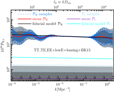
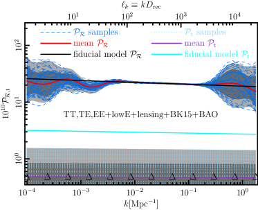
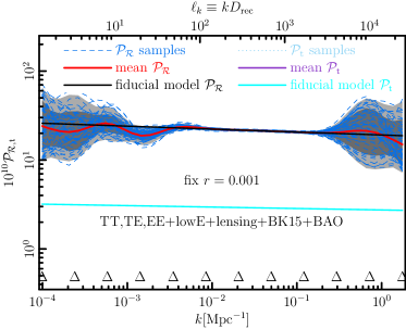
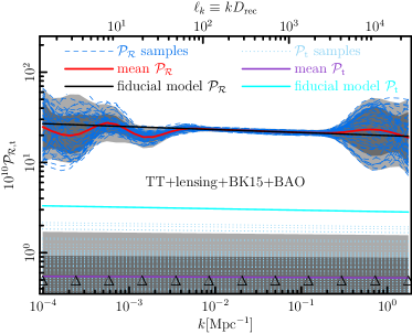
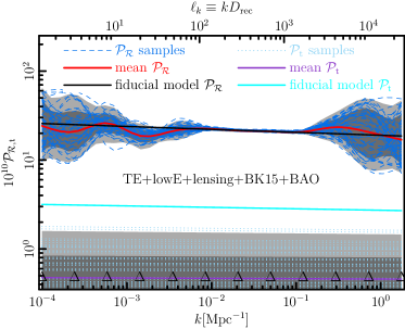
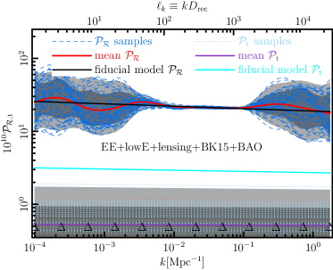
In spite of the extra scalar shape freedom in the -space region over which the tensor modes affect the CMB, the 12 knot reconstruction still leads to a strong constraint of , rather close to the limit obtained if the only shape parameter is . In fact we find that the current limits on are such that the scalar-power reconstructions are not sensitive to the details of the distribution. To illustrate this, the lower panel of Fig. 24 shows the spectrum when is fixed at the tiny value of . One could regard this as a theoretical prior for low-energy inflation models or a forecast for a future in which is measured or tightly constrained by -mode experiments.
In PCI15, the main cubic spline reconstruction included non-CMB data to help pin down cosmological parameters such as , , and the late-time expansion history. The improvements in the data from 2015 to 2018, especially the decreased errors on , result in no non-CMB data being needed. Although and are about 90 % correlated, as they are in the standard power-law model, neither are very correlated with the The strongest is about 40 % for at , corresponding to where reionization is kicking in. The second strongest is about for , similar to the correlation of and in the standard power-law model. (The correlations among the are also relatively small, except for the high bands and , where the data are not constraining.)
The middle panel in Fig. 24 shows the effect of adding the BAO constraint. Although apparently visually identical, there are slight differences. For example, the 1 error on at decreases by about , from to , while at the decrease is about . The restriction to does not change the error bars over the floating case. At intermediate for modes to the errors on are so close to zero that the reconstruction is quite compatible with a simple power law, corresponding to a straight line in Fig. 24. This was also a main result of the 2015 Planck reconstructions.
The errors on the grow above for as a consequence of increased cosmic variance, giving more freedom in the allowed trajectories. Unfortunately this is also the region of relevance to the power spectrum deficit in the – range. The most significant deviation from zero occurs for at : , , and for the three cases. Thus the anomaly in terms of deviation from the power law of the standard model hovers at around the level. More precisely, the 95 % upper confidence limits on are , , and , for the respective cases. This level of the anomaly was also the conclusion of the 2015 Planck reconstructions. Therefore, even though the low- deficit is robust against the various choices for the reconstruction, we conclude that it is not statistically significant. The associated , , , and power spectra responses to the allowed primordial power variations are derived from the mode expansion, and match the data well, in particular following the dip in at –.
In Fig. 25 we show the reconstructed power spectra using only the TT, TE, and EE data in conjunction with BK15. The fixed cases look very similar. Except at high , the polarization data using either EE or TE also enforce a nearly uniform over a broad range in , with values in excellent agreement with those obtained from TT alone, from TE and EE used in combination, and from the combined TT,TE,EE results. For example, the and errors at and , respectively, increase only slightly for TT only, to and , but, more significantly, to and with EE alone. The deficit region remains about the same, with the TT,TE,EE result for of quoted above changing slightly for TT alone, to , but with no hint of an anomaly for EE alone, at . If just the TE cross data are used, the values are closer to the TT case, namely, , now under a excursion from the tilted fiducial model.
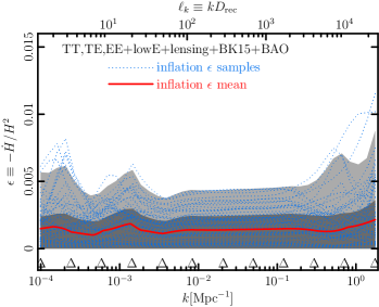
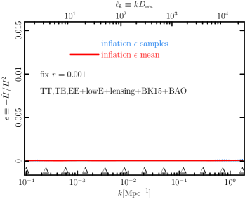
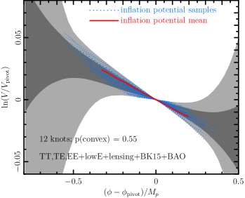
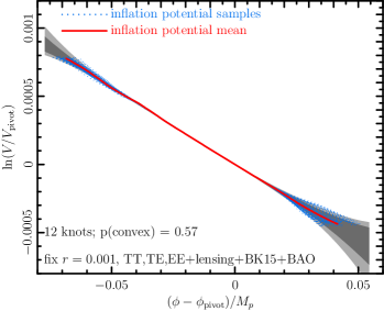
As in PCI15, we can use the and reconstructions to get an idea of the history of the acceleration of the Universe as a function of time over the significant number of -folds of the cosmic expansion that the CMB data probe, codified by the dynamical slow-roll parameter , considered as a function of , the value of the wavenumber at Hubble crossing. Results with floating and fixed to are shown in Fig. 26. For the dynamical time variable we use for the horizontal axis for ease in comparing with the curves of Fig. 24. The wide spread in the trajectories for the floating case is a consequence of being able to fit the shape by a combination of and . When is small, is almost entirely determined by , and the values cluster near .
The Hamilton-Jacobi energy constraint equation relates the potential to and via . Figure 27 shows the reconstructed inflationary potential shapes in the region over which the allowed inflationary potentials are constrained by the data for the floating and fixed cases. Instead of using for the horizontal axis, we translate into inflaton-field -space using the relation between and , referenced to the pivot position . For the vertical axis we plot , with the overall normalization removed. Its value is set by , hence there is a distribution of constant amplitudes to superimpose if we want the total . The radically different visual appearance for the floating and fixed cases is due to the observable range being compressed through the smallness of into a small precisely determined field range, whereas this range has a distribution in the floating case. One can monitor whether the shapes of the individual realizations of the potential trajectories bend upwards or downwards or do both, an indication of convexity. The sample trajectories shown are not exclusively convex or concave, and a measure of the probability that they are convex can be made from the ensemble. As indicated in Fig. 27 for the 12 knot case, the ensemble-averaged potentials are roughly exponential, with individual trajectories bending away from the mean, but with no strong tendency for convexity or concavity. (The roughly probability changes somewhat depending upon the combination of data used, whether TT,TE,EE or the individual data sets.)
The standard cosmological parameter determinations are highly robust to the addition of these spline shape degrees of freedom. The mean values change little and the error bars grow slightly, by around for , , and . The largest error increase is for with becoming . The main conclusions of this section on and , and , remain as in PCI15, but the results have been noticeably sharpened by the improvements in the Planck 2018 data sets.
7 Search for primordial features in the Planck power spectrum
The “bottom-up” power spectrum reconstruction methods of the previous section are an excellent way to search for coarse features in the spectrum, but lack the resolution to detect the higher-frequency features generically predicted by various physical mechanisms [see, e.g., Chluba et al. (2015) for a review]. It is therefore useful to complement power spectrum reconstruction with a “top-down” approach by fitting specific feature models to the data. In this section we will analyse a representative range of power spectrum templates which parameterize features in terms of a handful of new parameters.
With Planck’s temperature and polarization data, we have two essentially independent probes of features at our disposal and will pay particular attention to examining the consistency between the two (Miranda et al. 2015).
7.1 Power spectrum templates with features
| Log osc | Running log osc | Lin osc | Step | Kin cutoff | Rad cutoff | Kink cutoff | |
| [0,0.5] | [0,0.5] | [0,0.5] | |||||
| [0,2.1] | [0,2.1] | [0,2] | |||||
| [0,1] | [0,1] | [0,1] | |||||
| [,0.1] | |||||||
| [0,1] | |||||||
| [,] | |||||||
| [,5] | |||||||
| [,] | [,] | [,] | |||||
| [,0.7] |
7.1.1 Global oscillation models
Periodic or quasi-periodic modulations of the power spectrum which extend over the entire observable range of wavenumbers can occur in a variety of models [cf., e.g., Danielsson (2002); Martin & Brandenberger (2003); Bozza et al. (2003); Chen (2012); Jackson & Shiu (2013)]. A general parameterization of models with a sinusoidal modulation of the primordial power spectrum reads
| (58) |
where . Defining ,141414Throughout this section, we take . we consider the logarithmic oscillation model, given by , and the linear oscillation model, . In addition, we investigate a logarithmic model with running frequency, . For , this is a good approximation for the scalar power spectrum in the axion monodromy model (Flauger et al. 2017a), which will be analysed in more detail below, but here we allow for a wider range of the running parameter , including negative values (i.e., decreasing frequency with increasing ).
7.1.2 Localized oscillatory features: inflation with a step
A sudden transient event in the evolution of the inflation field, triggered by a sharp feature in the inflaton potential, or a sharp turn in field space, generically leads to a localized oscillatory feature in the power spectrum (Adams et al. 2001; Chen et al. 2007; Achúcarro et al. 2011; Miranda et al. 2012; Bartolo et al. 2013). As an example of this class of feature models, we consider here the case of a -step in an otherwise smooth inflaton potential (Adams et al. 2001), whose power spectrum can be parameterized as (Miranda & Hu 2014)
| (59) |
where the first- and second-order terms are given by
| (60) | ||||
| (61) |
with window functions
| (62) | ||||
| (63) |
and damping function
| (64) |
In this model, the parameter determines the amplitude of the oscillatory feature, the step scale sets the position of the step in -space, and the damping parameter determines the width of the envelope function.
7.1.3 Models with suppressed power at large scales
The apparent lack of power at the largest scales in the temperature power spectrum with respect to the expectation of base CDM serves as a motivation for models with a suppression of primordial perturbations below a cutoff scale . Physically, this effect may be due to fluctuations at the largest observable scales being generated at the onset of the inflationary phase after a prior era of, e.g., kinetic or radiation domination (Vilenkin & Ford 1982; Contaldi et al. 2003), or due to an isolated event such as a kink in the inflaton potential (Starobinsky 1992).
In these scenarios, the primordial spectrum can generally be analytically approximated by an expression of the form
| (65) |
with , where is a function with in the limit that describes the shape of the cutoff and the transition to a power-law spectrum at smaller scales.
Initial kinetic domination
If inflation is preceded by an era dominated by the kinetic energy of the inflaton field (i.e., fast roll), we have
| (66) |
with
| (67) | ||||
| (68) |
where denotes the Hankel function of the second kind (Contaldi et al. 2003).
Initial radiation domination
If inflation begins immediately after a radiation-dominated phase, the cutoff function reads (Vilenkin & Ford 1982)
| (69) |
Kink in the inflaton potential (Starobinsky model)
7.2 Data analysis
We employ a modified version of CAMB with suitably increased numerical precision settings to calculate the CMB angular power spectra for the feature models. Since variations of the primordial spectrum may be degenerate with late-time cosmology parameters (Obied et al. 2017), we explore a parameter space consisting of the base-CDM parameters and the respective additional free parameters of the feature models (see Table 11 for the prior ranges). Note that we take primordial tensor perturbations to be absent in our analysis. In the results presented in Sect. 7.3, nuisance parameters are assumed to be uncorrelated with the feature parameters and kept fixed to their base-CDM best-fit values.
In order to maximize sensitivity to narrow features, we use only the unbinned versions of the Planck high- likelihoods in the following combinations: (i) temperature data, Planck TT(unbinned)+lowE; (ii) -polarization data only, Planck EE(unbinned)+lowE; and (iii) temperature plus polarization data, Planck TT,TE,EE(unbinned)+lowE.
For all combinations of feature models and data, the parameter space is sampled with the nested sampling algorithm as implemented in MultiNest. The improvement in the fit due to the introduction of a feature is quantified by the effective . Being more complex than a power-law spectrum, feature models will in general have a negative . However, determining whether the improvement in fit is due to overfitting scatter in the data or due to an actual feature is not straightforward and requires model-dependent simulations (PCI15) or analytic estimates (Fergusson et al. 2015) to determine the expected under the null-hypothesis of an underlying power-law spectrum. In the Bayesian approach, a feature model’s general performance relative to base CDM can be expressed in terms of the Bayesian evidence (Trotta 2007a), which is also evaluated by MultiNest.
7.3 Feature candidates and their evidence
| Step | Kin cutoff | Rad cutoff | Kink cutoff | |||||||||
| TT | EE | TT,TE,EE | TT | EE | TT,TE,EE | TT | EE | TT,TE,EE | TT | EE | TT,TE,EE | |
| 0.0 | ||||||||||||
| 0.0 | 0.1 | 0.0 | 0.0 | 0.0 | 0.1 | |||||||
| 0.29 | 0.19 | 0.38 | ||||||||||
| 0.57 | 2.17 | 0.15 | ||||||||||
| 0.33 | ||||||||||||
| Log osc | Running log osc | Lin osc | |||||||
| TT | EE | TT,TE,EE | TT | EE | TT,TE,EE | TT | EE | TT,TE,EE | |
| 0.2 | |||||||||
| 0.024 | 0.073 | 0.014 | 0.028 | 0.082 | 0.016 | 0.024 | 0.046 | 0.015 | |
| 1.51 | 1.72 | 1.26 | 1.50 | 1.71 | 1.26 | 1.74 | 1.84 | 1.05 | |
| 0.60 | 0.07 | 0.07 | 0.68 | 0.62 | 0.11 | 0.34 | 0.81 | 0.56 | |
| 0.022 | |||||||||
We list the best-fit effective and Bayes factors with respect to a power-law spectrum in Tables 12 and 13. Examining the effective for the feature models previously considered in PCI15 reveals only minor differences, with a general trend towards smaller improvements due to features. The of the oscillation and step models fall well within the expected range of found in PCI15. Of note are the relatively high values of the radiation and kink cutoff models for polarization-only data, partially driven by the high quadrupole of the data. However, the best-fit parameters and spectra (see Fig. 30) do not match their counterparts in the temperature data at all, which strongly suggests that this is not a physical effect. The same observation can also be made for the step model: the best fit to the data is clearly out of phase with the temperature best fit.
We find a similar conclusion for the three oscillation models. As can be seen from the profile likelihood of the frequency parameters in Fig. 31, the likelihood peaks in the modulation frequencies do not match up between the TT and EE data sets. Furthermore, the preferred modulation amplitude for the EE data is in all cases much larger than that for the TT or TT,TE,EE data—given that the polarization data are noisier, this behaviour would be expected for a procedure that is overfitting the data.
Consequently, the Bayesian evidence for all combinations of models and data lies between barely worth mentioning and substantial evidence against the feature model on the Jeffreys scale. This implies that, currently, the Planck data do not show a preference for the feature models considered here.
Conversely, within the frequency ranges given by our priors, the relative modulation of the power spectrum is constrained to not exceed roughly , as shown in Fig. 28 for the logarithmic and linear oscillation models.
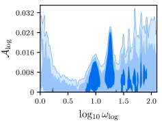
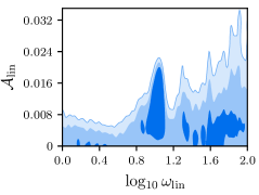
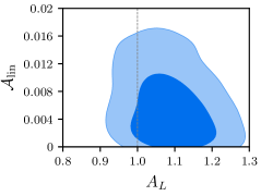
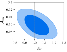
It may also be worth pointing out that in models with oscillations linear in , the wavelength of the corresponding modulation of the angular power spectra matches that of the CMB’s acoustic oscillations, , if . One might therefore suspect that features with frequencies around this value and carefully tuned amplitudes and phases could in principle mimic the (unphysical) effect of a lensing parameter, . However, for a model with a modulation at the BAO frequency and a -independent modulation amplitude , it can be seen in the left panel of Fig. 29 that we find no correlation between and . This is due to a different -dependence of the respective ’s. Explaining the lensing discrepancy would thus require a model with a carefully arranged scale-dependent linear modulation of the primordial spectrum. We demonstrate this possibility for a shaped modulation with a Gaussian envelope of the form in the right panel of Fig. 29, but it should be noted that this particular example is of course highly tuned to produce the desired effect.
Additionally, while the phenomenology of and linear modulation models is similar for temperature and polarization spectra individually, the two scenarios are in principle distinguishable by a combination of temperature and polarization data. This is due to the phase difference of the acoustic peaks in , , and , which leads to similar phase differences for the residuals when varying —unlike modifications of the primordial spectrum which do not shift phase in the same way. However, for features with an amplitude chosen to resemble the apparent lensing excess in the Planck TT data, the Planck TE and EE data are not sensitive enough to make this distinction.
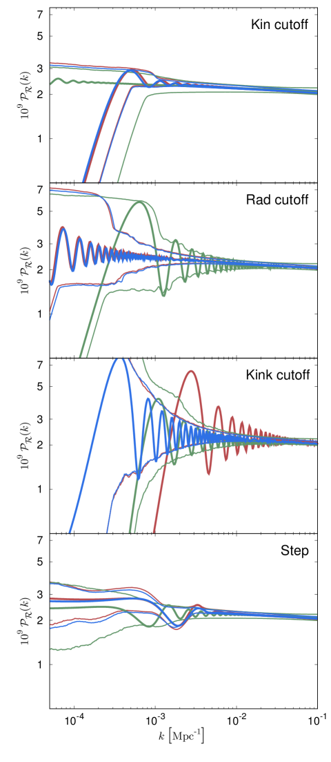
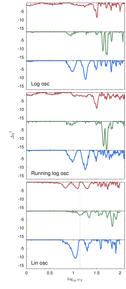
7.4 Axion monodromy
As in section 10.3 of PCI15, we next derive constraints on the underlying parameters in axion monodromy inflation (Silverstein & Westphal 2008; McAllister et al. 2010; Kaloper et al. 2011; Flauger et al. 2017a), which within string theory motivates a broad class of inflationary potentials of the form
| (71) |
where and are constants which have dimensions of mass, while , and are dimensionless. In the literature, one can find theoretically motivated models with and (Silverstein & Westphal 2008; McAllister et al. 2010, 2014). In the following, we neglect a possible amplitude drift in the modulation amplitude by fixing , focussing instead on a possible frequency drift , as was done in previous analyses (Peiris et al. 2013; Easther & Flauger 2014; Jackson et al. 2014; Meerburg & Pajer 2013; Meerburg et al. 2014c, a, b).
Due to its oscillating nature, a numerical study of this model is restrictive (Peiris et al. 2013). As such, we employ the semi-analytic template (Flauger et al. 2017a) used in previous analyses, namely
| (72) |
We neglect the effect of small oscillations in the tensor primordial spectrum, and approximate it as a power law with a very small spectral index (fixed by the single-field slow-roll self-consistency condition). The most well studied case to date is for , but given the high tensor-to-scalar ratio predicted by this model and the current upper bounds on given in Sect. 3.5, we extend our study to the cases of and . Furthermore, to completely specify this template, we assume instantaneous reheating, which, for a pivot scale of , corresponds to , and with . This leads to definite predictions for ; namely, for , for , and for .
To constrain this model, we carry out a Bayesian analysis using a modified version of CLASS (Lesgourgues 2011; Blas et al. 2011), which has been adapted to allow for a full parameter exploration, using the aforementioned template. As part of these modifications, special care needs to be taken to ensure that a correct sampling in wavenumber space is chosen, at two different levels in the Boltzmann code: when computing an interpolation table for the primordial spectrum of scalars and tensors; and when performing the integral over the squared photon transfer functions multiplied by the primordial spectra to get the multipoles . This sampling needs to be fine enough to guarantee that no features are smoothed out or lost in this convolution, and we checked carefully that this is the case in our runs. The grid of values at which the ’s are actually computed and not just interpolated also needs to be refined.
We fit to the data the five cosmological parameters plus the frequency of the underlying axion decay constant, the frequency drift , and the oscillation amplitude . We adopt the same priors used in previous analyses: for the frequency; for the frequency drift; and an upper bound on the amplitude of . Furthermore, for the phase parameter we take a uniform prior of .
In Figs. 32, 33, and 34 we show the joint posterior constraints on pairs of primordial parameters for the semi-analytic template, for , , and , respectively.
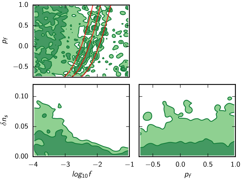
In all three cases, we find two expected asymptotic behaviours. First, when the frequency is very high (which means that is small in our parameterization), the oscillations in the primordial spectrum are smoothed out in the angular power spectrum, and the oscillation amplitude parameter becomes irrelevant and unconstrained. Second, in the limit of a very small amplitude parameter , the oscillations become undetectable and the parameter is also unconstrained. In all cases, no preferred frequency drift is found, which is compatible with previous analyses.
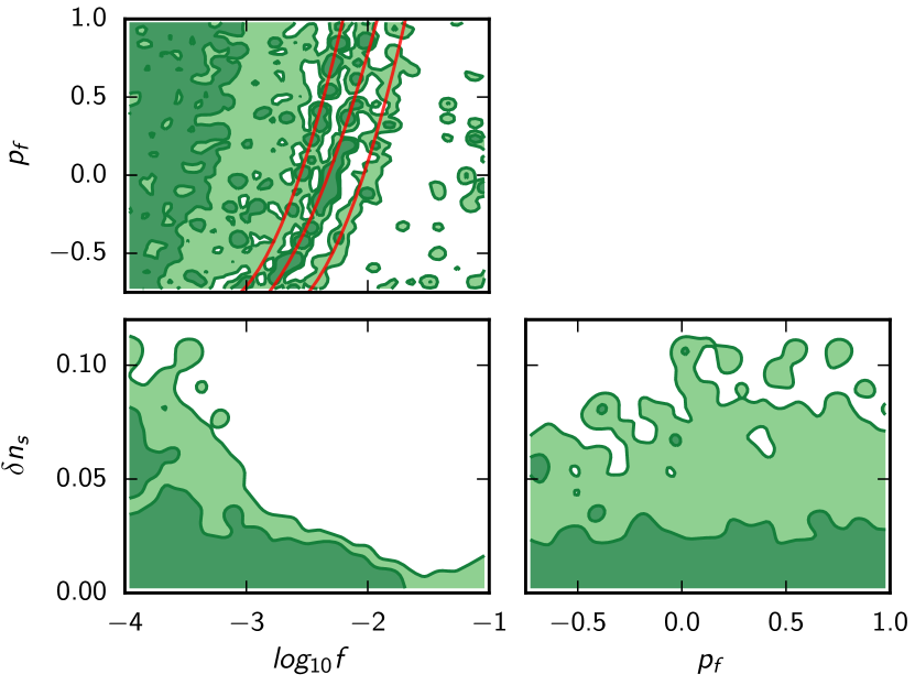
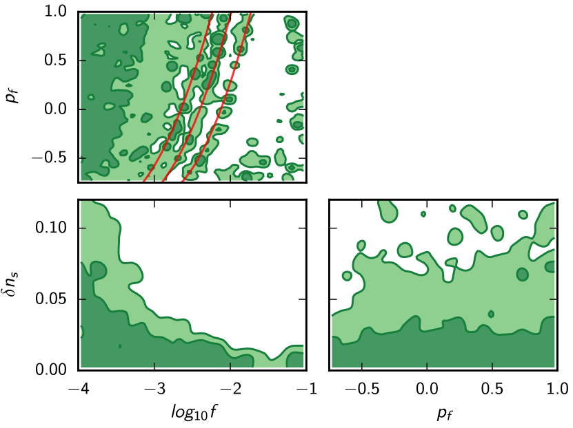
We recover the complex structures (highlighted in red in Figs. 32, 33, and 34) found in previous analyses in the frequency-frequency drift parameter space, which, as was discussed in PCI15, arise due to underlying modulations in the data and the model (Easther et al. 2005). These structures become more apparent as we reduce the index .
We perform a comparison with the minimal 6-parameter CDM model, and find , and . The reason for higher in the axion monodromy models, despite the addition of extra parameters, is that the predicted values are in tension with the CMB data. This shows that, overall, axion monodromy models are disfavoured due to their high tensor-mode amplitude.
In order to check specifically whether the data give any hint of oscillatory patterns in the primordial spectrum matching the axion monodromy template, as well as to compare with the results discussed in the previous subsection, we fitted the data with CDM+ models in which and were fixed to the same values as in the axion monodromy model with , , and . In each case, the comparison between axion monodromy and CDM+ with the same (, ) gives , and . That is, in all cases we find , which is compatible with the general results shown in Table 13. With three more free parameters, these improvements are statistically insignificant, and we conclude that the data show no preference for axion monodromy models.
8 Combined power spectrum and bispectrum analysis for oscillatory features
8.1 Approach
This section establishes constraints on oscillatory models using the power spectrum and the bispectrum simultaneously. Oscillatory features can appear in multiple correlation functions (Chen et al. 2008; Meerburg et al. 2009; Flauger et al. 2010; Flauger & Pajer 2011; Achúcarro et al. 2011; Adshead et al. 2012; Achúcarro et al. 2014; Flauger et al. 2017a, b) (see, e.g., Chluba et al. (2015) for a recent review). More powerful constraints result when spectra of various orders are combined (Palma 2015; Mooij et al. 2016; Gong & Yamaguchi 2017). Past work has suggested that the statistical weight of the oscillations in the bispectrum (or higher-order correlation functions) is less than that in the power spectrum (Behbahani et al. 2012); however, counterexamples exist as well (see, e.g., Behbahani & Green 2012). The analysis in Sect. 7 used the Planck data to establish stringent constraints on the presence of features in the power spectrum. The 2015 Planck data were analyzed to constrain non-Gaussianties containing features (Planck Collaboration XVII 2016), where, as in the power spectrum analysis, several candidate features were identified at low statistical significance. The analysis here focuses on the location, or frequency, of the feature. Joint analyses of the power spectrum and bispectrum were discussed in several studies (Fergusson et al. 2015, 2015; Meerburg et al. 2016). We apply some of the tools developed there to the Planck temperature and polarization data.
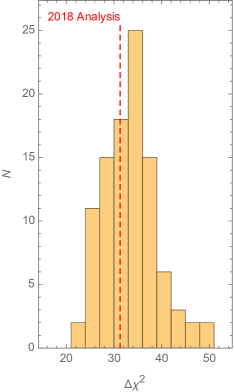
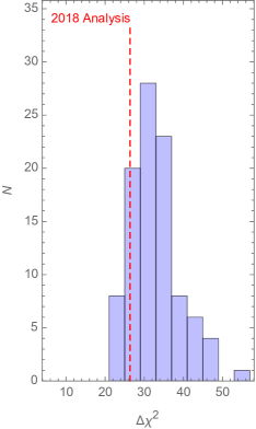
The analysis here is incomplete and limited in several respects. First, we analyse the bispectrum keeping all cosmological parameters fixed. Second, the parameters varied in the bispectrum are not varied in the Bayesian sense. The bispectrum is analyzed using a best-fit analysis based on how well a template shape fits the data. Third, the data suggest the primary bispectrum is close to zero and its covariance dominated by the scalar contributions in the power spectrum. We find that an ideal Bayesian analysis is not computationally feasible (see, e.g., Verde et al. 2013).
The output from the bispectrum analysis for features provides us with a map that specifies the significance of a feature in units of , given the location (frequency) and the phase of the feature. We can turn this map into a likelihood, which we can simply add to that of the power spectrum; in other words, we take
| (73) |
where represents the standard cosmological parameters, the foregrounds, the frequency, the amplitude, and the phase of the modulation in, respectively, the power spectrum and the bispectrum. We assume vanishing covariance between the power spectrum and the bispectrum, which has been shown to be a good approximation (Fergusson et al. 2015, 2015; Meerburg et al. 2016). Furthermore, the likelihood is not normalized (more precisely is not normalized in a universe with a non-zero bispectrum).
Strictly speaking, we do not have a likelihood that measures with a certain probability. Furthermore, several studies have shown that the frequency parameter, in combination with the amplitude and the phase, does not obey a fitting to the data (Hamann et al. 2010; Meerburg et al. 2014b, c, a; Meerburg 2014; Easther & Flauger 2014). Removing the frequency from the search results in a distribution with two degrees of freedom. Since is rather large (of order when combining all data), we can change the equation above by limiting ourselves only to improvements that are driven by , that is,
| (74) |
Assuming that and are well described by a two-parameter distribution, we can now convert our map into a improvement via
| (75) |
or, in terms of the likelihoods,
| (76) |
We will use the above expression to derive the posterior of the joint fit.
8.2 Models
We will focus on two models: the local or linear feature model and the log feature model. For the log model we set and use for the power spectrum
| (77) |
with . For the bispectrum we use (Chen 2010)
| (78) |
The above parameterized spectra are examples that could be generated in axion monodromy inflation (Flauger et al. 2010; Flauger & Pajer 2011), but generally are expected to appear in models where there exists an oscillatory potential.
For the linear model we follow (Fergusson et al. 2015) with and write
| (79) |
and (Chen et al. 2007)
| (80) |
In both models we choose Mpc-1, which is different from the choice in Sect. 7 for the linear model. As a result the linear frequencies can be related using . The pivot scale is set to the usual value Mpc-1. The above parameterization is a proxy for models that contain sharp oscillatory features (Chen 2010; Hu 2011; Adshead & Hu 2014), although typically such effects would generate decaying features, which will not be considered here.
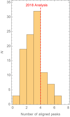
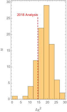
8.3 Data analysis
8.3.1 Power spectrum
Our analysis uses a modified version of CAMB (Lewis et al. 2000), which is capable of adaptively changing the sampling in both and depending on the frequency of the feature, allowing us to scan a wide range of frequencies. As in the previous section, we use the unbinned versions of the Planck high- likelihoods for temperature plus polarization, in combination with lensing and large-scale temperature and polarization (i.e., lowE). We compared the power spectrum results for the limited frequency range considered in Sect. 7 for the log and linear model, and find excellent agreement (sampled with Multinest). We developed a bispectrum likelihood module based on Eq. (76) using the 2015 data analysis (Planck Collaboration XVII 2016) for both the log and linear feature models, obtained using optimal estimators following Münchmeyer et al. (2014, 2015) and Meerburg & Münchmeyer (2015). For the log model, the frequency range is set to , while for the linear model we consider the frequency range . This joint analysis excludes the very low frequencies known to (weakly) correlate with cosmological parameters. The cosmological parameters are held fixed in the bispectrum analysis. We consider amplitudes ; the highest amplitudes will only be allowed for high frequencies where projection suppresses the power of the oscillating part in the power spectrum significantly. The phase is varied and marginalized over in the joint analysis. We use the PolyChord sampler (Handley et al. 2015a, b), which is powerful enough to include foregrounds (with ).
8.3.2 Bispectrum
The bispectrum likelihood is derived from the posterior distributions generated in Planck Collaboration IX (2018). Although the linear bispectrum of Eq. (80) can easily be factorized, the log bispectrum of Eq. (78) is not of the factorized form. Using modal techniques developed by Fergusson & Shellard (2009) and Fergusson et al. (2010, 2012), any shape can be factorized, with a close-to-optimal estimator. The modal method converts the angular-average bispectrum into a set of factorizable orthogonal mode functions. These functions can be directly constrained using foreground-cleaned CMB maps. From these measurements, a large number of bispectra can be reconstructed and constrained by appropriately weighting the mode functions. The convergence of this method, in terms of how many mode functions are required to accurately reconstruct the shape of interest, depends on the choice of the mode functions. In the 2015 analysis, two different mode functions were used: a polynomial-based reconstruction; and a trigonometric-based reconstruction. The latter was developed by Münchmeyer et al. (2014, 2015) and relies on expanding around linear oscillations. The polynomial-based reconstruction is extremely powerful for most bispectra, but is non-optimal for oscillatory bispectra, which require a large number of modes (e.g., more than for ). Trigonometric modes allow for faster convergence and provide good reconstruction for much higher frequencies, both for linear- and log-type modulations. For low frequencies, both methods can be compared and results show excellent agreement (Planck Collaboration XVII 2016). In addition, both methods were developed independently, which provides further confidence in the results. In the analysis presented here, we use the results obtained using the trigonometric mode functions. Further details can be found in Planck Collaboration IX (2018).
8.4 Estimating significance
Next we will estimate the significance of the improvements driven by the joint analysis. For this purpose we generate 100 mock spectra as in Meerburg et al. (2016) without features and perform an analysis jointly with true CMB power spectrum data, i.e., we use the same power spectrum likelihood (real data) in combination with the simulated bispectrum likelihoods (mock data). We will do this for both the linear and the log models, with 100 simulations in total. Each analysis requires a similar amount of time as does the real data analysis, using about CPU hours for the linear feature and about CPU hours for the log feature per simulation. More details on the simulated spectra can be found in (Planck Collaboration IX 2018).
These simulations help us assess the statistical significance of our results. Improvement in fit is given in units of compared to a no-feature model as defined the previous section [i.e., ]. The left panel of Fig. 35 shows the typical best-fit improvement from a set of simulations for the log feature model. This first analysis shows that the best fit in the data is perfectly consistent with a standard CDM universe, without features, with . This outcome is not unexpected, given earlier analyses for the power spectrum (see, e.g., Meerburg et al. 2014c; Easther & Flauger 2014; Benetti 2013; Miranda & Hu 2014; Fergusson et al. 2015; Planck Collaboration XX 2016; Hazra et al. 2016) and the significance of features in the bispectrum alone (Planck Collaboration XIII 2016). The look-elsewhere effect lowers the significance of features and by jointly constraining features in the power spectrum and the bispectrum it is possible to alleviate some of this suppression. To quantify this, we consider the following two questions: 1) considering the various frequencies with improvement over no features in the joint analysis, how many of those were present in the power spectrum analysis only; and 2) what is the mean improvement, in units of , of these fits? We compare the results of the simulations, which do not contain any real features, to the data.
Before we answer these questions we need a criterion to decide if two frequencies will be considered the same or not, i.e., we need a frequency correlation measure. We will consider a simple ansatz, which will have an analytical solution and will serve to estimate the correlation between frequencies, by defining
| (81) |
Next we marginalize over phase, defining
| (82) | ||||
| (83) |
where . For linear oscillations we can derive a similar measure, with
| (84) |
The correlation is given by
| (85) |
The parameters and play a role in determining the correlation length. Although strictly speaking they correspond to the minimum and maximum scales observable in the CMB, they can be used to model the correlator to allow for shifts in the frequency coming from a non-optimal analysis. We argue that this is reasonable given the low number of peaks in the analysis. We tested the above on various nearby peaks in the data and found that demanding is generally sufficient to effectively identify independent peaks. We explored the sensitivity of the results to the correlation criterion of 0.1. First we increased it to 0.3 and found that in this case many peaks were missed when counting the number of aligned peaks (with little effect on determining the peaks). When we lowered the criterion to 0.01, we obtained many aligned peaks that should not be aligned. Small changes in the correlation criterion have minimal effect on the results presented here. Ideally, more simulations should be generated, which would help to establish the best choice for the correlation criterion. We found that the choice of does not affect the correlator as long as . We set for linear oscillations, which roughly correlates peaks with , which is within the tails of the observed widths of the peaks in the power and bispectrum analysis. For log oscillations we choose , which has the advantage that the correlator has no zero-crossings near the peak (but hardly effects the correlation length). We find at , which seems reasonable in light of the power and bispectrum peak widths (see Fig. 31).
In Fig. 36 we show the number of peaks in the joint analysis that have improved (left panel) as well as their mean improvement (right) over a no-feature analysis. We find and those peaks do not lead to significant improvements in the joint , with . Assuming that these 100 simulations provide a fair sample of the noisy data, we conclude that there are no significant features present in both the power spectrum and the bispectrum for the models considered within the chosen range of feature parameters.
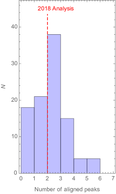
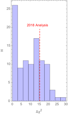
We carry out the same analysis for linear features and show the results in Fig. 35 (right panel), deriving a typical best fit from 100 simulated noisy spectra. The true best fit, as derived from the joint analysis of the 2018 bispectrum and the 2018 power spectrum, shows a relatively small improvement with . Further correlated-features searches find 2 features within the frequency window which may be considered aligned, with a mean of 12.3, as illustrated in Fig. 37. Compared to 100 simulated noisy spectra, we obtain and . Since the overall improvement from fitting these aligned peaks does not exceed the threshold, we conclude that there is no statistically significant evidence for any of these features.
We conclude that the simple parameterization considered in this analysis does not provide any evidence for features. The two models analyzed are representive of a broad class and have well-studied phenomenological spectra; however, other classes of models exist. Features, for example, can have scale dependence [i.e., an “envelope” (Chen 2010; Achucarro et al. 2014; Torrado et al. 2017)]. Likewise, more realistic modelling of axion models shows that the frequency could depend on scale [i.e., “running” (Flauger et al. 2017a, b)]. Both these possibilities could substantially change the spectra and likely the joint analysis and significance.
Here we have not imposed an explicit relation between the amplitude of the bispectrum and the frequency of the power spectrum. In the simplest form of axion monodromy, one has . On account of the quadratic scaling with frequency and the fact that the constraint on the amplitude tends to become poorer as the frequency increases due to projection (see, e.g., Fig. 32), it was already pointed out in Planck Collaboration XX (2016) that there is no evidence for this relation in the data, and with the current data set this situation remains unchanged.
9 Constraints on isocurvature fluctuations
| at | ||||||||
| Model and data | ||||||||
| General models (three isocurvature parameters): | ||||||||
| CDI Planck 2015 TT+lowP | ||||||||
| CDI Planck TT+lowE | ||||||||
| CDI CamSpec TT+lowE | ||||||||
| CDI Planck TT+lowP | ||||||||
| CDI Planck TT + prior | ||||||||
| CDI Planck 2015 TT+lowP+lensing | ||||||||
| CDI Planck TT+lowE+lensing | ||||||||
| CDI CamSpec TT+lowE+lensing | ||||||||
| CDI Planck 2015 TT,TE,EE+lowP | ||||||||
| CDI Planck TT,TE,EE+lowE | ||||||||
| CDI CamSpec TT,TE,EE+lowE | ||||||||
| CDI Planck TT,TE,EE+lowP | ||||||||
| CDI Planck TT,TE,EE + prior | ||||||||
| CDI Planck TT,TE,EE+lowE+lensing | ||||||||
| CDI CamSpec TT,TE,EE+lowE+lensing | ||||||||
| CDI Planck TT,TE,EE+lowP+lensing | ||||||||
| CDI WMAP-9 | ||||||||
| NDI Planck 2015 TT+lowP+lensing | ||||||||
| NDI Planck TT+lowE+lensing | ||||||||
| NDI Planck TT,TE,EE+lowE+lensing | ||||||||
| NVI Planck 2015 TT+lowP+lensing | ||||||||
| NVI Planck TT+lowE+lensing | ||||||||
| NVI Planck TT,TE,EE+lowE+lensing | ||||||||
| CDI+ Planck TT+lowE | ||||||||
| CDI+ Planck TT+lowE+lensing | ||||||||
| CDI+ Planck TT,TE,EE+lowE | ||||||||
| CDI+ Planck TT,TE,EE+lowE+lensing | ||||||||
| Special CDI cases (one isocurvature parameter): | ||||||||
| Uncorrelated, | ||||||||
| “axion I” Planck 2015 TT+lowP+lensing | ||||||||
| “axion I” Planck TT+lowE+lensing | ||||||||
| “axion I” Planck TT,TE,EE+lowE+lensing | ||||||||
| Fully correlated, | ||||||||
| “curvaton I” Planck 2015 TT+lowP+lensing | ||||||||
| “curvaton I” Planck TT+lowE+lensing | ||||||||
| “curvaton I” Planck TT,TE,EE+lowE+lensing | ||||||||
| Fully anti-correlated, | ||||||||
| “curvaton II” Planck 2015 TT+lowP+lensing | ||||||||
| “curvaton II” Planck TT+lowE+lensing | ||||||||
| “curvaton II” Planck TT,TE,EE+lowE+lensing | ||||||||
| Special CDI cases (two isocurvature parameters): | ||||||||
| Uncorrelated, free | ||||||||
| “axion II” Planck TT+lowE+lensing | ||||||||
| “axion II” Planck TT,TE,EE+lowE+lensing | ||||||||
| Arbitrarily correlated, | ||||||||
| “curvaton III” Planck TT+lowE+lensing | ||||||||
| “curvaton III” Planck TT,TE,EE+lowE+lensing | ||||||||
| Fully correlated, free | ||||||||
| Planck TT+lowE+lensing | ||||||||
| Planck TT,TE,EE+lowE+lensing | ||||||||
| Fully anti-correlated, free | ||||||||
| Planck TT+lowE+lensing | ||||||||
| Planck TT,TE,EE+lowE+lensing | ||||||||
(a)
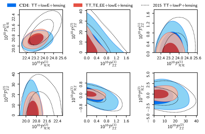
(b)
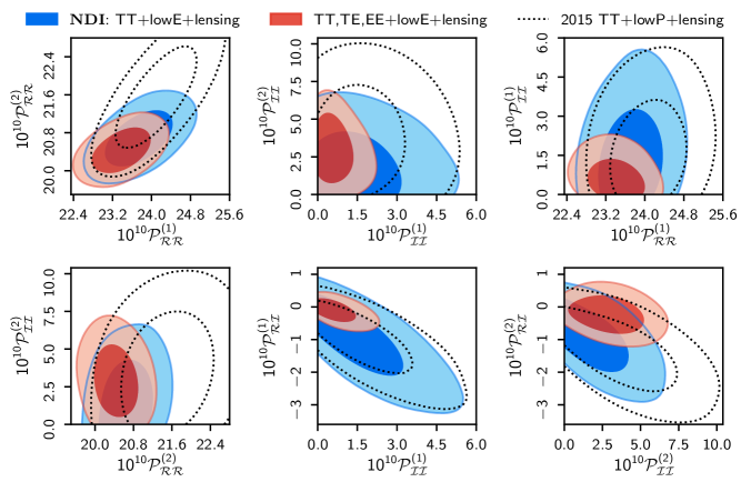
(c)
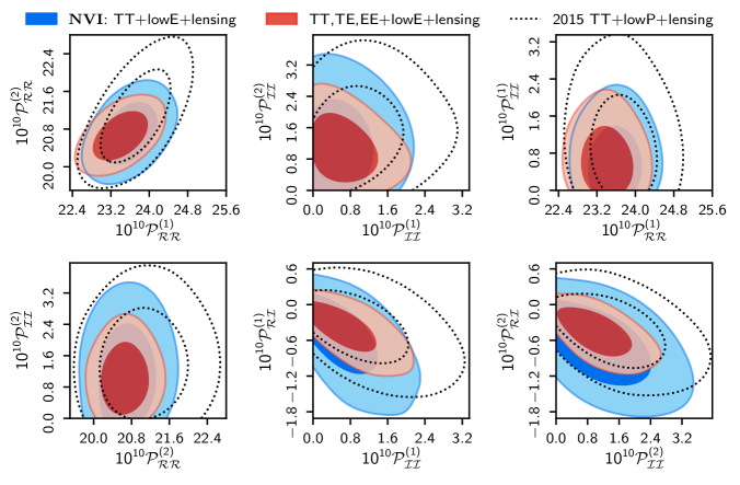
(a)

(b)

(c)

9.1 Background and modeling
Single-field inflation with a canonical kinetic term gives rise to primordial super-Hubble comoving curvature perturbations, . In this case the relative number densities of the various particle species are spatially constant, i.e., the perturbations are adiabatic. Typically photons are chosen as a reference species. Then adiabaticity implies that for every particle species with number density the quantity vanishes. However, in addition to , multi-field inflation can stimulate isocurvature modes, , where at primordial times varies spatially (Linde 1985; Polarski & Starobinsky 1994; Linde & Mukhanov 1997; García-Bellido & Wands 1996). In this section we consider all possible non-decaying modes of this type (Bucher et al. 2000): cold dark matter density isocurvature (CDI); baryon density isocurvature (BDI); and neutrino density isocurvature (NDI) modes. For completeness, we also constrain the fourth non-decaying mode, neutrino velocity isocurvature (NVI), although there are no known mechanisms to excite it. Finally, we consider compensated isocurvature perturbations (CIP) between baryons and CDM (Grin et al. 2011a, b). In this case, opposite BDI and CDI perturbations cancel in such a way that the total matter isocurvature perturbation vanishes and there is no first-order isocurvature signal in the CMB. However, we utilize a higher-order lensing-like effect from this mode to obtain constraints on CIP from Planck temperature and polarization power spectra. We find the most powerful power-spectra-based constraints on this mode by exploiting the cosmological information in the low- lensing potential reconstruction in Sect. 9.5, but leave the use of Planck trispectra in constraining CIP for future work.
As the positions of the peaks and dips of the CMB angular power spectra in the density isocurvature models are roughly in opposite phase compared to the pure adiabatic (ADI) spectrum, the primordial CDI, BDI, and NDI modes leave a very distinctive observational imprint on the CMB, whereas the imprint of the NVI mode more closely resembles the pure ADI mode; see, e.g., figure 43 in PCI15. Prior to the detection of CMB anisotropies, studies such as Peebles & Yu (1970) and Efstathiou & Bond (1986, 1987) discussed the possibility that isocurvature perturbations were the sole source of cosmological fluctuations. However, at least after the detection of the first acoustic peak in , it became clear that the density isocurvature mode(s) had to be subdominant (Enqvist et al. 2000, 2002), while the adiabatic mode led to a good agreement with observations. Several pre-Planck isocurvature constraints were obtained (Stompor et al. 1996; Pierpaoli et al. 1999; Langlois & Riazuelo 2000; Amendola et al. 2002; Peiris et al. 2003; Valiviita & Muhonen 2003; Bucher et al. 2004; Moodley et al. 2004; Beltran et al. 2004; Kurki-Suonio et al. 2005; Dunkley et al. 2005; Bean et al. 2006; Trotta 2007b; Keskitalo et al. 2007; Komatsu et al. 2009; Valiviita & Giannantonio 2009).
The mixture of curvature and isocurvature perturbations can be uncorrelated, but typically an arbitrary amount of correlation arises between them if the trajectory in field space is curved between Hubble radius exit and the end of multi-field inflation (Gordon et al. 2001). In extreme cases, such as the simplest curvaton models, there is full correlation or full anticorrelation between and . In the following subsections, we start with the generic case of generally correlated adiabatic and CDI, NDI, or NVI perturbations. Then we deal with various special CDI (or BDI) cases with no correlation or full (anti)correlation.
We parameterize the primordial perturbations as in PCI15, following the notation described there. The primary perturbation parameters scanned by MultiNest (in addition to the four standard CDM background cosmological parameters and the Planck nuisance parameters) are the primordial abiabatic perturbation power and isocurvature perturbation power at two scales, corresponding to Mpc-1 and Mpc-1, namely, , , , , and the correlation power between and at , i.e., . We assume a power-law form for the adiabatic and isocurvature power spectra and denote the spectral indices that can be calculated from the primary parameters by and . The correlation spectrum is also assumed to obey a power law, with spectral index . Thus is not an independent parameter. This ensures that the correlation fraction stays inside the interval at every , as long as we reject any which does not obey this requirement. While the correlation fraction is -independent in our modelling, the primordial isocurvature fraction depends on , unless . We also report at an intermediate scale, Mpc-1.
We do not separately quote constraints on BDI or the total matter density isocurvature (MDI), since these modes are observationally indistinguishable from the CDI case.151515If we assume no NVI or NDI perturbations, then the MDI perturbation (i.e., the spatial perturbation in the relative number densities of matter particles and photons) is (86) As we will see, the posteriors for and are insensitive to the assumed initial conditions. Thus it is a good approximation to use the mean values obtained in the generally correlated mixed adiabatic and CDI model with TT,TE,EE+lowE+lensing data, namely , , , and . For example, to convert our CDI upper bound on to a BDI bound, we should multiply the constraint by , and to convert the CDI to BDI, we should multiply the constraint by . If , then this also can be converted to a BDI constraint by multiplying the CDI constraint by . The constraint on will be the same for the CDI and BDI cases, since the conversion factor cancels out.
Numerical results for various isocurvature models and selected derived parameters are reported in Table 14, utilizing various data combinations. The table is divided into three main sections: generally correlated models (discussed in Sect. 9.2); one-isocurvature-parameter CDI models (discussed in Sects. 9.4.1 and 9.4.2); and, finally, two-isocurvature-parameter CDI models (discussed in Sects. 9.4.3, 9.4.4, and 9.4.5). For generally correlated CDI we study the stability of constraints (see Sect. 9.3) by using several different subsets of the Planck data: (1) only high- TT; (2) high- TT+lensing; (3) TT,TE,EE; and (4) TT,TE,EE+lensing. For comparison, some Planck 2015 and WMAP results are also cited. Table 14 also includes comparisons to the pure adiabatic model in terms of the difference in the best-fit and the natural logarithm of the Bayesian evidence (“model probability”) ratios , negative being evidence against the mixed models.161616The values of depend on the priors. We adopt uniform priors in the range for the adiabatic, for the isocurvature, and for the primordial correlation power parameter.
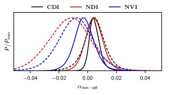
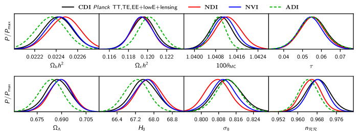
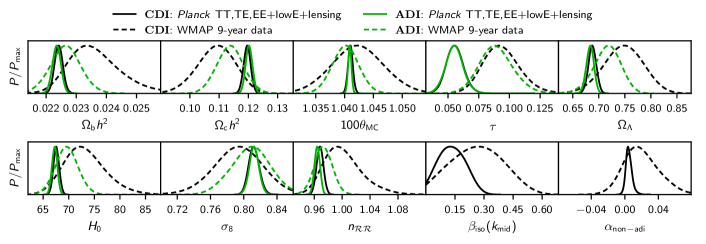
9.2 Results for generally correlated adiabatic and isocurvature modes
This subsection explores mixed adiabatic and isocurvature models where only one isocurvature mode at a time is considered. We consider the CDI, NDI, and NVI modes using the Planck 2018 TT(,TE,EE)+lowE(+lensing) data. All five primordial perturbation power amplitudes (of which three describe the isocurvature perturbations) are free parameters. It follows that and are independent and varies between and . The constraints for the primary perturbation parameters and the derived parameter are shown in Fig. 38.
In all three cases the Planck TT+lowE+lensing results are very similar to the previous results from the Planck 2015 TT+lowP+lensing likelihood. As expected, the lower value of preferred by the 2018 (lowE) data is reflected in the adiabatic amplitudes and . For CDI and NDI there is no significant shift in the constraints on isocurvature parameters, but we find slightly tighter constraints than in 2015. For NVI, a minor shift towards more negative correlations is observed (see the last two panels of Fig. 38c). As in 2015, adding the high- TE,EE data significantly tightens the constraints in all three cases.
When fitting the generally correlated three-isocurvature-parameter models, the Planck data are consistent with null detection, i.e., with the pure adiabatic model, and (and ). The natural logarithm of the ratio of model probabilities [i.e., the Bayes factor ] is below , corresponding to odds of less than 1 : for all three (CDI, NDI, NVI) models. If there were an undetected subdominant isocurvature contribution to the primordial perturbations, a negative correlation between and would be favoured, in particular for NDI and NVI (see the last two panels of Figs. 38a,b,c). With our sign convention, this leads to a negative contribution to the Sachs-Wolfe effect and hence reduces the amplitude of the temperature angular power spectrum at low multipoles.
Figure 39 updates the 2015 Planck constraints on the derived primordial fractions and spectral indices. At large scales we find with Planck TT,TE,EE+lowE+lensing that for the CDI, for the NDI, and for the NVI model, all at 95 % CL. Figure 40 shows the non-adiabatic fraction in the observed CMB temperature variance, defined as
| (87) |
where
| (88) |
The non-adiabatic fraction is below 1.7 % with Planck TT,TE,EE+lowE+lensing data for all three cases at 95 % CL.
Since the Planck data do not allow a significant isocurvature contribution, the determination of standard cosmological parameters depends only very weakly on the assumed initial conditions, as seen in Fig. 41. We place this result in historical perspective in Fig. 42 (and Table 14) where the parameter determinations of the mixed CDI model and the pure adiabatic model are compared to the pre-Planck constraints set by the WMAP 9-year data.171717The pivot scales and used here to parameterize the primary perturbation amplitudes are not optimal for WMAP, since the WMAP data extend only to . Nevertheless, an analysis tailored to WMAP [see Savelainen et al. (2013), who used as an upper pivot ] gives a similar posterior range for Planck has dramatically tightened the constraint on the adiabatic spectral index. Its value is now below unity (scale-invariance) in the pure ADI case. Allowing for generally correlated CDI reduces the significance of this detection only slightly, to , whereas the WMAP 9-year data were consistent with a blue tilt as large as at 95 % CL. The non-adiabatic contribution to the CMB temperature variance is constrained (about zero) 5 times more tightly than by WMAP. Finally, the allowed range for the sound horizon angle has shrunk by a factor of in the CDI case, thanks to the Planck data covering more acoustic peaks beyond the first three peaks detected by WMAP.
9.3 Role of lensing parameter and likelihood choices
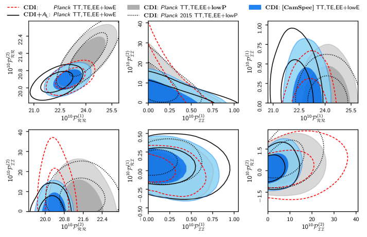
The small-scale primordial CDI amplitude is extremely sensitive to the details of the high- temperature and polarization power spectra and to choices made in constructing the likelihoods. Therefore the general CDI model serves as a robustness test of the Planck data and likelihoods. We now discuss a few curious aspects related to CMB lensing and likelihoods.
Lensing smooths the peaks of the CMB power spectra. This effect is taken into account in our theoretical predictions for the mixed adiabatic and isocurvature models by first calculating the total unlensed CMB spectra as a sum of adiabatic, isocurvature, and correlation ’s, and performing a similar summation for the lensing potential power spectrum (Seljak 1996; Lewis & Challinor 2006). The total lensing potential is then used to lens the total CMB spectra. Starting with the WMAP data, accounting for CMB lensing became necessary for calculating constraints on isocurvature models, as Valiviita et al. (2012) showed that there is a strong degeneracy between the lensing effect and the CDI contribution in the generally correlated mixed models. Fixing or (as is done in the next subsection) makes this degeneracy disappear. This is because in these models the CDI contribution modifies only the low- part of the angular power spectra. The transfer function mapping the primordial CDI mode to the (and ) angular power is suppressed by a factor relative to the adiabatic mode. Therefore, to be observable at high , the CDI mode must be blue tilted (). A blue-tilted CDI mode affects the total angular power spectra in a manner somewhat similar to lensing. Since the acoustic peaks of the CDI mode have the opposite phase compared to the adiabatic mode, a CDI admixture can “smooth” the peaks and dips of adiabatic acoustic oscillations. The NDI mode does not have precisely the opposite phase and is not damped relative to the adiabatic mode (see figure 43 in PCI15). Thus we expect a weaker impact of lensing on the primordial NDI amplitude than in the CDI case. Therefore in this subsection we explore the general CDI model as an example.
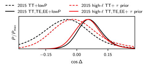
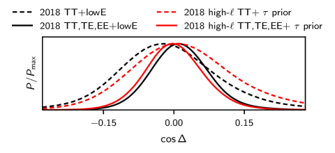
Starting with the Planck 2013 release, the consistency of the smoothing effect with the adiabatic CDM model has been routinely tested by multiplying the lensing power spectrum by a phenomenological lensing consistency parameter, , prior to lensing the unlensed CMB spectra (Calabrese et al. 2008). The expectation is that . However, the Planck temperature and polarization data prefer a higher level of lensing-like smoothing () than expected in the adiabatic CDM model. In the 2018 release (PCP18) we have
| (89) | |||||
| (90) |
Adding the Planck CMB lensing likelihood pulls these constraints towards (see also Table 15). The measurement of when TT,TE,EE data are included depends on the calibration of the polarization channels. This procedure and the details of the sky masks differ between the Planck baseline Plik TT,TE,EE and the alternative Planck CamSpec TT,TE,EE likelihood, as discussed in PPL18 and PCP18. The Planck CamSpec TT,TE,EE likelihood prefers a smaller value of than Plik, but still lying about above unity.
Given the above motivation, we check the response of the generally correlated CDI model to the various possible choices of likelihoods available in the Planck 2018 release, and, on the other hand, we gauge how the baseline Plik likelihood reacts when allowing to vary. For clarity, in Fig. 43 we restrict the analysis to high- TT,TE,EE and low- TT,EE(,BB) data without the lensing reconstruction data, but in Table 14 we also report TT+lowE and TT+lowP results, and include Planck lensing in some cases.
We notice a considerable variation in the constraints on the isocurvature power at high , , which corresponds to the high- region in the observed power spectra. In Fig. 43 we can compare the red dashed reference contours (obtained with the Planck baseline Plik TT,TE,EE+lowE likelihood) for the CDI model (where ) with the solid black contours (obtained with the same data) for the CDI+ model, where is allowed to vary. In many cases, adding an extra free parameter is expected to weaken the constraints on the other parameters, but in this case adding tightens the 95 % CL constraint on by a factor of from to . This is reflected in the derived primordial isocurvature fraction , whose upper bound changes from to , according to Table 14. Therefore, we conclude that, when , the CDI mode partially accounts for the extra lensing-like smoothing effect required by the Planck TT(,TE,EE) data. Once we allow the lensing amplitude to vary, there is not much need for the CDI contribution at high , which should be kept in mind when interpreting the results. In Table 14 we report four cases where is allowed to vary. In all the other cases we have fixed . In these cases the constraints at high are “conservative”, i.e., weaker than the Planck data were expected to be capable of (Finelli et al. 2018), due to CDI (or NDI) partially fitting the lensing anomaly. Furthermore, again comparing the red dashed and black solid contours, we observe a slight weakening of the constraint for in the CDI+ model. This is due to the rigidity of the assumed power-law spectrum. When the high- data allow much less CDI, the low- (low-) CDI amplitude can be larger without much affecting the middle- range of the CMB power spectra between the first and third acoustic peaks, which is the most sensitive region to departures from adiabaticity. (This is the same see-saw effect discussed in the end of Sect. 3.6 in the case of tensor perturbations.) Finally, in the panel we see a minor shift toward smaller amplitudes, which is an indication of the well-known degeneracy between and the overall primordial perturbation amplitude.
From Table 14 it is obvious that adding the lensing data reduces the differences discussed above. This is again as expected, since the lensing data favour values of only mildly above unity. For example, with Planck TT,TE,EE+lowE+lensing we obtain for CDI+ and for the CDI model.
We now proceed to a comparison of the likelihoods. The grey shaded contours in Fig. 43 indicate the results for the same CDI model as the red dashed contours, but changing the low- likelihood from the combination Commander TT+SimAll EE to the LFI 70 GHz pixel-based low T,E,B, which is by its methodology and construction very similar to the 2015 baseline low- likelihood (dotted contours). Indeed, this can be seen in the results: most of the isocurvature parameters follow more closely the 2015 results with this likelihood combination than with the 2018 baseline. This implies that when it comes to isocurvature, not much has changed in high- TT. 2018 lowP favours slightly smaller values of the optical depth than the 2015 version, hence the small shift towards smaller values of the adiabatic amplitude in the panel. With respect to the red dashed contours, the grey contours prefer higher adiabatic amplitudes and have a long degeneracy line in the plane. This is due to lowP having a higher central value and larger uncertainty on .
Finally, the blue shaded contours in Fig. 43 represent the results when using the CamSpec likelihood, to be compared to the red dashed contours obtained by the baseline Plik likelihood. All the other parameters shown are relatively stable against the high- likelihood, but stands out. CamSpec leads to an upper bound of , whereas the baseline Plik result was , or for versus at 95 % CL, according to Table 14. This difference is not surprising, given the different responses of these likelihoods to in the adiabatic CDM+ model, and keeping in mind the –CDI degeneracy in the CDI model. However, this difference is not as concerning as it might appear at first sight: all the cases shown in Fig. 43 are fully consistent with zero isocurvature. It is only the upper bound that varies, with the baseline Plik likelihood and CDI model with leading to the most conservative (i.e., weakest or safest) upper bounds.
For CDI the 2015 release Planck high- TT data favoured a negative correlation fraction but the preliminary high- TT,TE,EE data favoured a slightly positive correlation. This was confirmed using only the high- Plik likelihood (and a prior on ), as shown by the red curves in the top panel of Fig. 44. Including the low- data (black curves) did not significantly alter this tension between TT and TT,TE,EE results. In the present 2018 Planck release this tension has disappeared. Both high- TT and TT,TE,EE data lead to a correlation fraction posterior peaking at zero, as demonstrated in the bottom panel of Fig. 44. Including the low- TT data (black dashed curve) still shifts the posterior slightly towards negative values, due to the low power at low multipoles in the data.
9.4 Specific CDI models
In this subsection we constrain CDI models with only one or two isocurvature parameters. The two-parameter cases were not studied in the 2013 and 2015 Planck releases.
First we fix to unity and assume no correlation between the CDI and adiabatic modes (“axion”), or we fix and assume full (anti)correlation between the CDI and adiabatic modes (“curvaton I/II”). These models are less sensitive to any residual systematic effects in the high- data (such as the determination of polarization efficiencies or foreground modeling) than the generally correlated models, since CDI now modifies the angular power spectra insignificantly at (see figure 43 in PCI15). As seen in the middle section of Table 14, the Bayesian evidence values for the one-parameter extensions of the adiabatic CDM model are higher than for the three-parameter extensions, but all Bayes factors fall below . None of the one-parameter extensions improve over the adiabatic CDM model. The two-parameter extensions in the bottom section of Table 14 are even more strongly disfavoured, except for the uncorrelated case with free (“axion II”), which is actually the only model that improves the best-fit by slightly more than the number of extra parameters.
9.4.1 Uncorrelated ADI+CDI (“axion I”)
Particularly insensitive to any data is the “axion I” case, since the CDI transfer function has a suppression and there is no correlation component whose amplitude would be higher than that of the isocurvature alone and hence would modify the adiabatic spectrum. The “axion I” case is achieved in our parameterization by setting and . Thus the only varied isocurvature parameter is . This uncorrelated case with is a good approximation for many multi-field inflationary models where the slow-roll parameter (in the isocurvature field perturbation direction) is negligible and the background trajectory in field space is straight between Hubble radius exit and the end of inflation. The predictions for the spectral indices (to first order in the slow-roll parameters) are and , where and is the second slow-roll parameter in the “adiabatic” direction (i.e., along the trajectory) in the field space. (An exact match with our model would require .) The axion model [see, e.g., a recent review by Marsh (2016) and references therein], which was originally proposed to solve the strong CP problem and provides a dark matter candidate, can produce this type of isocurvature modes with under the following assumptions (\al@planck2013-p17,planck2014-a24; \al@planck2013-p17,planck2014-a24): the Peccei-Quinn symmetry should be broken before inflation; it should not be restored by quantum fluctuations of the inflaton nor by thermal fluctuations when the Universe reheats; and axions produced through the misalignment angle should form a significant fraction of the dark matter.
Table 14 indicates a slight tightening of the “axion I” constraints using TT+lowE+lensing with respect to 2015 TT+lowP+lensing. This is due to the change of the baseline low- data from the 2015 LFI 70-GHz pixel-based T,E,B to the 2018 combination of Commander TT and SimAll EE, which in the generally correlated cases also gave tighter constraints at low . As expected, the addition of high- TE,EE data only marginally improves the constraints, since the standard (non-isocurvature) parameters are better constrained now. For uncorrelated CDI, we obtain
| (91) |
Using equation (73) of PCI13, we convert the constraint on the primordial isocurvature fraction to a bound on the inflationary energy scale. If all the dark matter is in axions, the above constraint corresponds to the same limit we quoted in 2015, that is,
| (92) |
where is the expansion rate at Hubble radius exit of the scale corresponding to and is the Peccei-Quinn symmetry-breaking energy scale.
9.4.2 Fully (anti)correlated ADI+CDI (“curvatonI/II”)
If , the low- data are maximally sensitive to the fully correlated isocurvature perturbations. In this case the correlation component is a geometric average of the adiabatic and isocurvature components, and hence much larger than the isocurvature component alone. We achieve this case in our parameterization by setting and , i.e., . The only isocurvature parameter to be varied is again . Since , the derived isocurvature fraction is independent of . A physically motivated example of this type of model is the simplest curvaton model, where a light scalar field that is subdominant (and hence irrelevant for the inflationary dynamics) starts to oscillate at the bottom of its potential after the end of inflation, causing its average energy density to evolve like non-relativistic matter. Once fully (or almost fully) dominating the energy density of the Universe, this curvaton field decays either to CDM or to other species (Mollerach 1990; Linde & Mukhanov 1997; Enqvist & Sloth 2002; Moroi & Takahashi 2001; Lyth & Wands 2002; Bartolo & Liddle 2002; Lyth et al. 2003). The amount of isocurvature and non-Gaussianity present after curvaton decay depends on the “curvaton decay fraction,” , evaluated at curvaton decay time. Under a number of (very) restrictive assumptions discussed in PCI15, the curvaton model can lead to fully (anti)correlated CDI (or BDI) and adiabatic perturbations.
Not surprisingly, both in the fully correlated and anticorrelated cases, the constraint on is much (about 40 times) stronger than in the uncorrelated case. At 95 % CL, Planck TT,TE,EE+lowE+lensing leads to
| (93) | ||||
| (94) |
both rounded to in Table 14. As in 2015, the TT data favour anticorrelation, due to the low power in the low- temperature compared to the expectation of the adiabatic CDM model. But when the TE,EE data (which do not particularly favour negative correlation) are added, a very tight (one part per thousand) constraint on the primordial isocurvature fraction results.
Fully correlated perturbations are obtained, e.g., in case 4 described in Gordon & Lewis (2003). Many models giving anticorrelation produce too large an isocurvature fraction to be consistent with the above limit, but case 9 of Gordon & Lewis (2003) survives. After the curvaton decay, the primordial isocurvature fraction in these models will be , where for the fully correlated CDI case and for the fully anticorrelated CDI case, and is the CDM fraction of the total non-relativistic matter.
On the other hand, the nonlinearity parameter describing non-Gaussianity is (Sasaki et al. 2006)
| (95) |
where is the small-scale variance of the curvaton perturbations, or the ratio of the energy density carried by the curvaton particles to the energy density of the curvaton field (if there is significant production of curvaton particles). The parameter cannot be smaller than , which is obtained when and , as implicitly assumed, for example, in Bartolo et al. (2004a, b). The above limits correspond to the following and constraints (assuming ):181818The quoted precision of these constraints does not reflect the precision of the sampling of the likelihood surface, but we report several digits here since the constraints are so tight that rounding to, e.g., two significant digits would give empty or almost empty ranges.
| (“curvaton I”) | ||||
| (96) | ||||
| (“curvaton II”) | ||||
| (97) | ||||
Even with the maximal allowed isocurvature fraction, the local non-Gaussianity in the curvaton model is well within the observational Planck limits presented in Planck Collaboration IX (2018). The residual isocurvature peturbations in the two studied curvaton models set much tighter constraints on the curvaton decay fraction than do constraints on the observed (consistent with zero) non-Gaussianity.
9.4.3 Uncorrelated ADI+CDI with free (“axion II”)
Axion models do not necessarily produce nearly scale-invariant isocurvature perturbations. In particular, even highly blue-tilted spectra (in the observable CMB range) are possible. For example, Kasuya & Kawasaki (2009) construct a model with –. This motivates studying a two-isocurvature-parameter model, where adiabatic and isocurvature modes are uncorrelated, but the isocurvature fraction and spectral index are free to vary. In our parameterization this is achieved by setting , and varying and independently. The results for this model are presented in the first two rows of the third section of Table 14. The low- temperature data do not favour any extra contribution beyond the (already too high) abiabatic contribution, whereas the fit to the high- temperature and polarization data can be improved slightly by the “smoothing” caused by the CDI mode. This leads to a very blue isocurvature spectrum. Planck TT,TE,EE+lowE+lensing gives at 95 % CL , consistent with the recent findings of Chung & Upadhye (2017). Even the very large upper bound corresponds to a contribution of less than order to the observable CMB (or ) power spectra at . The uncertainty in the Planck spectrum at these high multipoles is K2 and the actual spectrum is K2. Thus the allowed CDI contribution is only of the same order as the observable uncertainty. Consequently the non-adiabatic contribution to the observed CMB temperature variance, , is also vanishingly small, between and .
9.4.4 Arbitrarily correlated ADI+CDI with (“curvaton III”)
Apart from the extremes of correlation, some curvaton models predict an arbitrary degree of correlation. The generic feature of most curvaton models is that the isocurvature and adiabatic spectral indices are equal. This is because both perturbations typically arise from the same source. In the next-to-simplest models, the correlation fraction can be written as , where . Therefore, the model is fully correlated only if , in which case the results of “curvaton I” apply. If the slow-roll parameter is very close to zero or the curvaton field value is large compared to the Planck mass, this model leads to almost uncorrelated perturbations and the constraints are well approximated by “axion I.” Any other case leads to an arbitrary degree of positive correlation between the CDI and adiabatic modes.
Modulated reheating with thermal or non-thermal production of gravitinos can lead to positive or negative correlation, respectively (Takahashi et al. 2009). While the correlation could in principle be arbitrarily large, the observational constrains on favour only small correlations.
Arbitrarily correlated ADI+CDI with is also a good approximation for those two-field (or multi-field) slow-roll models [e.g., double quadratic inflation (Langlois 1999; Beltrán et al. 2005)] where the trajectory in field space is curved between the Hubble radius exit of perturbations during inflation and the end of inflation. The fraction of isocurvature perturbations converted to adiabatic depends on how the trajectory is curved and this part of the adiabatic perturbations will be fully (anti)correlated with the isocurvature modes, whereas the adiabatic perturbations already present at Hubble radius exit are uncorrelated with isocurvature modes to first order in the slow-roll parameters, and only slightly correlated to second order. [See, e.g., Gordon et al. (2001), Amendola et al. (2002), van Tent (2004), and Byrnes & Wands (2006).] The result is a non-zero correlation between isocurvature and total adiabatic perturbations. The spectral indices of both components are typically , which is well approximated by since the data indicate .
As expected, the Planck data favour negative correlations, since these models modify only the low- part of the CMB spectra, where power is lower than predicted by the adiabatic CDM model. With TT,TE,EE+lowE+lensing we find, at 95 % CL, and .
9.4.5 Fully (anti)correlated ADI+CDI with free
The remaining two-parameter CDI extensions of the adiabatic CDM model are those where the perturbations are fully (anti)correlated, as in the simplest curvaton models, but the isocurvature spectral index is not fixed to the adiabatic one. In this case the free isocurvature parameters are and , while . These models are somewhat difficult to motivate, since full (anti)correlation typically implies that the curvature and isocurvature perturbations have their origin in (the decay products of) the same field. Then one would expect equal spectral indices, as in the curvaton model. The conversion of isocurvature perturbations to adiabatic ones (e.g., between Hubble radius exit and the end of inflation, or by curvaton-type decay, or by reheating/thermalization) should be scale dependent in order to obtain . Slow-roll two-field inflation leads to an exact match, , in the case where . [See, e.g., Byrnes & Wands (2006)]. Nevertheless, for completeness we report constraints on these phenomenological models in the last four rows of Table 14. Since the low- TT data favour negative correlation, a larger isocurvature fraction is allowed in the fully anticorrelated case at low . This leads to scale-invariant isocurvature perturbations being in the favoured region of parameter space, namely with TT,TE,EE+lowE+lensing at 95 % CL. In contrast, in the fully correlated case the low- TT data disfavour any isocurvature contribution, and hence prefer a blue spectrum, with .
9.5 Compensated BDI–CDI mode
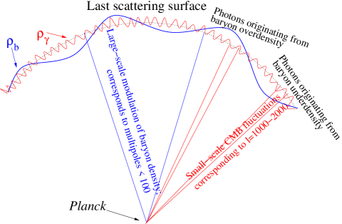
This subsection presents constraints on uncorrelated adiabatic and scale-invariant CIP modes and discusses the strong degeneracy between the phenomenological lensing parameter and the CIP amplitude (Valiviita 2017). Assuming that there are no NVI or NDI perturbations, the total matter density isocurvature perturbation , given by Eq. (86), vanishes if
| (98) |
This mode, where the anticorrelated CDI and BDI perturbations cancel even though their individual amplitudes can be large, is called a compensated baryon and cold dark matter isocurvature mode. The CIP mode does not leave a linear-order isocurvature signal in the CMB or matter power spectra (Gordon & Lewis 2003), although it modifies the trispectrum (Grin et al. 2011a, 2014). However, at the next order there is a smoothing effect on the high- , , and spectra. A formal derivation can be found, for example, in Smith et al. (2017). Here we summarize the heuristic arguments of Muñoz et al. (2016).
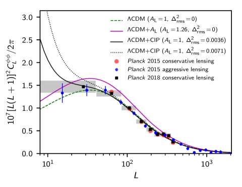
On scales larger than the sound horizon, condition (98) is preserved until last scattering and can be written as
| (99) |
Consequently, CIP can be described as a large scale modulation of the baryon and CDM density (Muñoz et al. 2016; Heinrich et al. 2016; Valiviita 2017), with
| (100) |
Here the overbar denotes an average over the whole sky and a small perturbation about this average in the direction , as illustrated in Fig. 45. In patches of sky where the CMB photons originate from baryon-overdense regions, the odd acoustic peaks at high- are more pronounced relative to the even peaks compared to the patches where the photons originate from baryon-underdense regions. Averaging over the sky leads to a lensing-like smoothing of the high- peaks.
A convenient measure of CIP is the variance . If is a Gaussian random variable, the observed angular power of , , or will be
| (101) | |||
where and . For brevity, we will denote the power spectrum in the integrand by . For each it can be calculated by assuming adiabatic initial conditions. Approximating the integrand by the first three terms of its Taylor series about , we end up with
| (102) |
In the following we describe parameter scans where we vary the six standard (adiabatic) CDM parameters, the Planck nuisance parameters, and the CIP variance , calling this one-parameter extension of the CDM model the “CDM+CIP” model. We evaluate the right-hand side of Eq. (102) at each point in parameter space using a finite-difference approximation for the second derivative:
| (103) |
where should be “sufficiently small.” In practice, good numerical accuracy is achieved if is of order . So at each point in our MultiNest scan we set for the point currently under evaluation, and thus the result of Eq. (102) simplifies to
| (104) |
With this method each angular power spectra evaluation takes twice as long as for the pure adiabatic case since the spectra are now an average of two spectra, resulting from different values of and .191919Actually, we call CAMB three times (i.e., also with and , or ), in order to obtain some auxiliary parameters such as correctly, although we do not report them here.
Unlike the high- , , and spectra, the high- lensing potential power spectrum is virtually unaffected by CIP. Instead, CIP modifies the low multipoles of by, approximately, adding a term . For details, see table II in Smith et al. (2017). As illustrated in Fig. 46, when using the Planck 2015 conservative lensing data () this term does not affect the results. In contrast, the Planck 2018 conservative lensing data also contain the range and thus CIP variances fit the first data point of the 2018 lensing power spectrum () worse than in CDM. However, even in this case the joint fit of the CDM+CIP model to the TT, TE, EE, and lensing data is better than that of the CDM model, the improvement being of the same order as for the CDM+ model.
| Constraints | Best fit | |||||
|---|---|---|---|---|---|---|
| Data and model | ||||||
| TT+lowE | ||||||
| CDM+CIP | 15.5 | 1.00 | ||||
| CDM+ | 0.0 | 1.26 | ||||
| CDM++CIP | 3.4 | 1.23 | ||||
| TT,TE,EE+lowE | ||||||
| CDM+CIP | 10.0 | 1.00 | ||||
| CDM+ | 0.0 | 1.19 | ||||
| CDM++CIP | 0.3 | 1.19 | ||||
| TT,TE,EE+lowE+lensing (conserv.) | ||||||
| CDM+CIP | 3.6 | 1.00 | ||||
| CDM+ | 0.0 | 1.07 | ||||
| CDM++CIP | 2.9 | 1.07 | ||||
| TT,TE,EE+lowE+lensing (aggr.) | ||||||
| CDM+CIP | 2.7 | 1.00 | ||||
| CDM+ | 0.0 | 1.05 | ||||
| CDM++CIP | 2.4 | 1.06 | ||||
The top panel of Fig. LABEL:fig:CIP2d shows the – degeneracy in the CDM++CIP model and how it can be broken by the lensing data. The value provides a good fit to the TT+lowE data, if , and to the TT,TE,EE+lowE data, if . The CDM+CIP model (where ) with provides a better simultaneous fit to the Planck 2015 TT,TE,EE and conservative lensing data () than does the CDM+ model. When using the Planck 2018 conservative lensing data (), the best-fit value of decreases to . This is due to the extra term brought by CIP to the lensing power estimator, as discussed above and shown in Fig. 46.
Since Planck TT,TE,EE+lowE and lensing data can be fit well by in the CIP model, we show in the bottom panel of Fig. LABEL:fig:CIP2d the one-dimensional posterior of in the CDM+CIP model. A non-zero value of is preferred at the () level by Planck 2018 (2015) TT+lowE(lowP) data and at the () level by the TT,TE,EE+lowE(lowP) data. Without lensing the 2018 data thus more strongly favour the non-zero CIP amplitude than the 2015 data, which is as we would expect, since the favoured value in the CDM+ model has also increased. When using 2018 TT,TE,EE+lowE and the 2018 conservative lensing data the significance decreases to , while switching to the aggressive lensing data () leads to . The 68 % CL ranges of in the CDM+CIP model, obtained with the baseline high- Plik likelihood in combination of other Planck data, are highlighted in Table 15. Replacing Plik with CamSpec (in particular CamSpec TT,TE,EE) leads to somewhat lower values,
| (105) |
and reduced significance above zero: , , , and , respectively.
In order to check that the preference for or is not just a parameter-space volume effect upon marginalization over other parameters, we also report in Table 15 the difference of between the best fit in extended models and the base adiabatic CDM model. With all data sets, all three extended models lead to an improvement of which clearly exceeds the number of extra parameters of the model (1 for CDM+CIP and CDM+, and 2 for CDM++CIP). Although the inclusion of lensing data reduces this improvement of fit, the CDM+CIP model gives a rather impressive with Planck TT,TE,EE+lowE and aggressive lensing data.
Since we observe a moderate preference for a non-zero CIP amplitude, it might be tempting to “solve” the Planck lensing anomaly by using CIP. However, this explanation seems quite unlikely, since in our treatment the CIP and adiabatic perturbations should be uncorrelated with each other, whereas CDI and BDI should be fully anticorrelated (and have a few orders of magnitude larger amplitude than the adiabatic modes while keeping the perturbations nearly Gaussian). It is difficult to imagine a physical model that could lead to this situation. For example, some variants of curvaton model would naturally lead to anticorrelated CDI and BDI, but in these models there would be a correlation with the adiabatic mode too (Gordon & Lewis 2003; He et al. 2015). The above-studied compensated BDI-CDI mode falls into a similar category to NVI: it is an interesting theoretical setup, but a compelling early-Universe model for stimulating this mode has still to be discovered.
Nevertheless, the baseline Planck Plik TT,TE,EE+lowE plus conservative lensing result, , is fully compatible with current complementary observations, in particular, the WMAP 95 % CL trispectrum constraint, (Grin et al. 2014), and the upper bound, , following from the direct measurements of the variation of the baryon fraction in galaxy clusters (Holder et al. 2010; Grin et al. 2014). It will be interesting to learn what other future CMB anisotropy (Abazajian et al. 2016; Valiviita 2017; Finelli et al. 2018) and complementary measurements, such as observations of the distribution of neutral hydrogen using 21 cm absorption lines (Gordon & Pritchard 2009), BAO (Soumagnac et al. 2016, 2018), or CMB spectral distortion anisotropies (Haga et al. 2018), will tell us about the possible contribution of CIP to the primordial perturbations.
10 Constraints on anisotropic models of inflation
In this section we will test specific physical models for statistical anisotropy in the primordial fluctuations. More phenomenological multipole- or map-space tests are performed in the companion paper, Planck Collaboration VII (2018). Here we update the results of the 2015 release (PCI15) with polarization and new temperature analyses. Incorporating polarization into these tests is particularly important, due to the mild statistical significance of temperature anomalies such as the dipolar asymmetry. Polarization offers the potential to confirm or refute a physical origin for such anomalies via the measurement of independent fluctuation modes. We perform such a new test with -space dipolar modulation models. In cases such as quadrupolar asymmetry, where no detection has been claimed with temperature, polarization offers the prospect of tightening existing constraints.
Some asymmetry models predict a modification to the isotropic power spectra, in addition to a dipolar or quadrupolar asymmetry. In other words, for these models, as well as non-zero off-diagonal multipole covariance elements, we expect departures in the diagonal elements relative to the standard CDM prediction. Therefore the isotropic spectra can provide independent tests of such models even using temperature data alone (Contreras et al. 2018). The curvaton dipole modulation model we examine in Sect. 10.1.1 exhibits this property, and can be constrained via its predictions for isotropic isocurvature power. Similarly, some versions of the quadrupolar modulation model we study in Sect. 10.2 modify the isotropic spectra via a monopole term. In both cases these isotropic constraints will be important in narrowing the viable parameter space.
10.1 Dipolar asymmetry
A dipolar temperature power asymmetry has long been observed at the largest scales in the CMB (Eriksen et al. 2004), although its statistical significance is not high and is subject to a posteriori (look-elsewhere) corrections (Bennett et al. 2011; Planck Collaboration XXIII 2014; Planck Collaboration XVI 2016). Nevertheless, its large-scale character suggests potential links with inflationary physics and various models have been proposed to explain it. In this subsection we examine several physical models for a dipolar modulation. Some models where a generic CDM density isocurvature (CDI) or tensor component is dipole modulated have already been ruled out due to their isotropic predictions (Contreras et al. 2018), so we do not consider these further here.
10.1.1 Curvaton model
First we update our 2015 study (PCI15) of a specific inflationary model for the dipolar asymmetry: namely, the modulated curvaton model of Erickcek et al. (2009). In that study we showed that that model could not explain the observed asymmetry. Here, we generalize the curvaton model to allow for a non-scale-invariant uncorrelated CDI component. In addition, we treat the power spectrum (isotropic) constraints in a fully unified way with the asymmetry likelihood. Finally, we incorporate polarization.
The modulated curvaton model employs a gradient in a background curvaton field to explain the observed large-scale power asymmetry. The curvaton, via coupling , produces nearly scale-invariant CDI fluctuations, as well as a fraction, , of the adiabatic fluctuations. Both of these components will be modulated. Up to a sign, is equal to the correlation parameter, and is also a measure of the amplitude of dipolar modulation. The isocurvature fraction can be written in terms of these two parameters as
| (106) |
Full details of this model and our treatment of it can be found in Erickcek et al. (2009) and PCI15.
Using the dipolar asymmetry estimator from PCI15 we find the posteriors for the dipolar modulation parameters and ; the results are presented in Fig. 48 (red contours). We see that a substantial amount of asymmetry (as measured by amplitude ) can be captured by the model. This preference for asymmetry simply means that the curvaton model can explain the well-known dipolar asymmetry in temperature. However, isocurvature constraints from the power spectra via Eq. (106), which we refer to as the isotropic constraints, can provide independent information (Contreras et al. 2018). This is also shown in Fig. 48, with the blue contours. Here we see that the asymmetry and isotropic posteriors only weakly overlap, and the independent isotropic data do not support the presence of asymmetry for this model. No evidence for asymmetry (i.e., no preference for ) is present in the joint constraints, which treat the isotropic and asymmetry data as independent. In other words, we have no reason to prefer this model over base CDM.
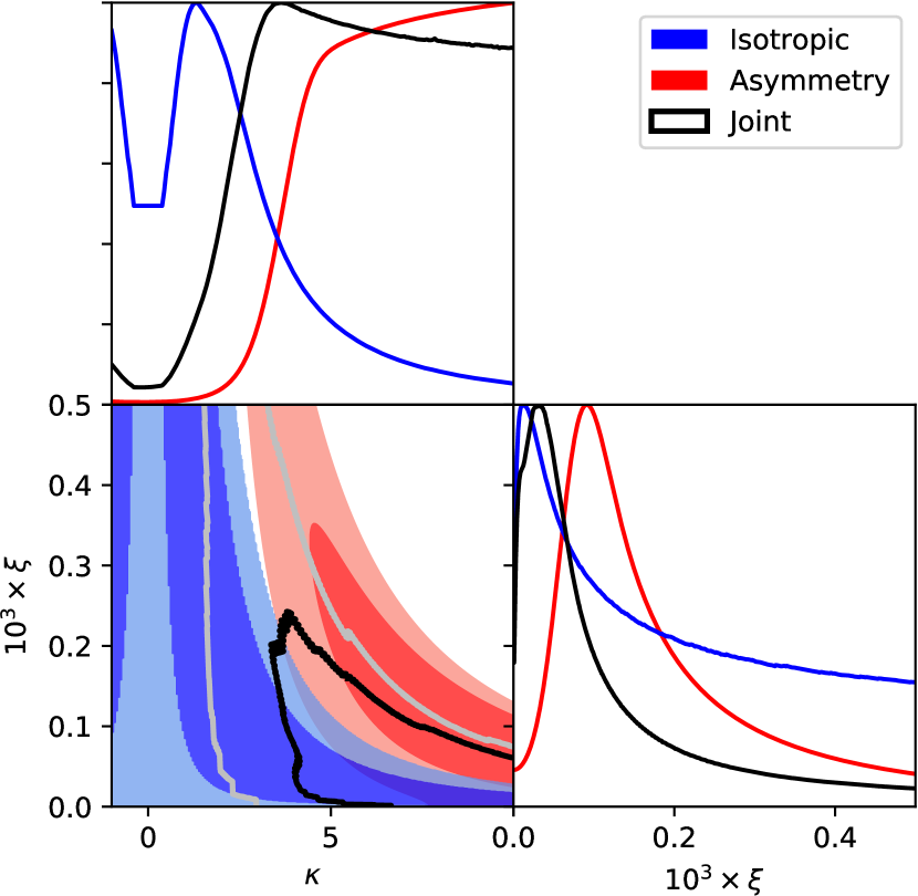
10.1.2 Adiabatic models
In the presence of a sufficiently large bispectrum it is possible that a long-wavelength mode can induce a dipolar asymmetry in the two-point function across our observable volume, although such scenarios appear to require fine tuning (Byrnes et al. 2016b). Nevertheless, examples have been constructed which satisfy the Planck constraints (Byrnes et al. 2016a). In this subsection we consider adiabatic models of this type, in which the isotropic power spectra agree with standard CDM, while a scale-dependent dipolar asymmetry is present in the off-diagonal multipole covariance (Contreras et al. 2017, 2018). As proposed in Contreras et al. (2017), we fit the asymmetry model parameters to the temperature data and then use those parameters to predict the asymmetry in polarization. We then compare those predictions with the Planck polarization data as a test for a physical modulation. Importantly, a position- (or -) space model for the modulation is needed for reliable polarization predictions—it is not enough to restrict considerations to multipole space (Contreras et al. 2017).202020E.g., if we observe a dipolar modulation in at, say, 5 % to , there is no reason to expect a modulation of the same amplitude and to the same scale in , due to the different and transfer functions (Contreras et al. 2017).
As discussed in detail in Contreras et al. (2017), we take a portion of the adiabatic primordial fluctuations to be spatially linearly modulated according to
| (107) |
where is statistically isotropic with power spectrum , and are the amplitude and direction of modulation, respectively, and is the comoving radius to last scattering. This leads, to a good approximation, to the total temperature or polarization multipole covariance
| (108) | ||||
| (109) |
to first order in . Here is the usual CDM anisotropy power spectrum; , where is the power spectrum calculated in the usual way from ; is the multipole decomposition of ; and the coefficients couple to via
| (110) |
In principle the scale dependence of the asymmetry spectrum is completely free, but here we take three phenomenological forms which are capable of producing a large-scale asymmetry with a small number of parameters. First, we consider a simple power-law modulation,
| (111) |
where is the usual CDM spectrum, and and are the tilt and pivot scale of the modulation. We consider only red asymmetry tilts with , and choose . We also consider a model, defined according to
| (112) |
This spectrum approaches that of CDM on scales larger than , with a width determined by . That is, scales well above the cutoff will be modulated with amplitude , and scales below will be unmodulated. Finally, we consider a model with a linear gradient in the scalar tilt, , across our volume. In this case the asymmetry spectrum can be written as
| (113) |
with modulation amplitude . There will be an implicit dependence on the pivot scale for this model.
Given the multipole covariance, Eq. (109), we can construct a maximum likelihood estimator for the modulation, . In the noise-free, full-sky case this takes the form (Moss et al. 2011; Planck Collaboration XVI 2016)
| (114) |
where the cosmic variance of the estimator is given by
| (115) |
The modifications we use to deal with realistic skies are described in detail in Planck Collaboration XVI (2016) and Contreras et al. (2017).
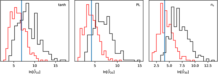
To decide whether the polarization data support the modulation model or not, we consider the quantity , which is the ratio of the maximum likelihood for modulation model to that of CDM (Contreras et al. 2017). In Fig. 49 we plot for the three adiabatic models histograms of calculated for 300 statistically isotropic polarization simulations (sharing the required correlation with the real data) added to the Planck temperature data (red outlines). This indicates our expectation for for the scenario that the temperature asymmetry is due to a statistical fluctuation and not to a physical modulation. We also plot in Fig. 49 histograms for 300 polarization simulations modulated with the best-fit parameters from the Planck temperature data (black outlines), to represent the scenario that the asymmetry is due to a physical modulation. In both cases the polarization simulations contain realistic levels of noise for Planck. By comparing the isotropic and modulated histograms, we can see that the quantity can serve to distinguish the two scenarios, but only relatively weakly for Planck noise (Contreras et al. 2017). The blue lines indicate the values using the actual SMICA polarization data (the results for the other component-separation methods are similar). We see that for these models the data do not help to decide whether we have a physical modulation or not, with -values of , , and for the power-law, , and gradient models, respectively, relative to the isotropic simulations.
10.2 Quadrupolar asymmetry
We will next explore models that predict a quadrupolar direction dependence in the primordial power spectrum. In PCI15 we found no evidence for such a modulation, but several inflationary models have been constructed which predict this effect (Ackerman et al. 2007; Soda 2012; Tsujikawa 2014). Therefore it is important to extend those results with the improved polarization data. We now attempt to reduce the effect of unresolved point sources using the bias-hardened estimator approach of Planck Collaboration XV (2016). In PCI15 we pointed out that some models of quadrupolar asymmetry predict a modification to the angular power spectra as well. Here we will account for such modifications in our analysis, increasing the constraining power of temperature data, in particular for tilted models with non-scale-invariant modulation spectral index. Note that independent searches relaxing our approximation of power-law spectra have also been carried out (Durakovic et al. 2018).
We assume a modulation of the primordial comoving curvature power spectrum of the form
| (116) |
which can be rewritten as
| (117) |
Here
| (118) |
with satisfying . We parameterize the scale dependence of the modulation as , with pivot scale . For , in addition to producing a quadrupolar modulation of the anisotropies, this model affects the CMB isotropic power spectra via the term in Eq. (117). We therefore consider a joint constraint with the isotropic power spectra likelihood to improve constraints over the modulation alone.
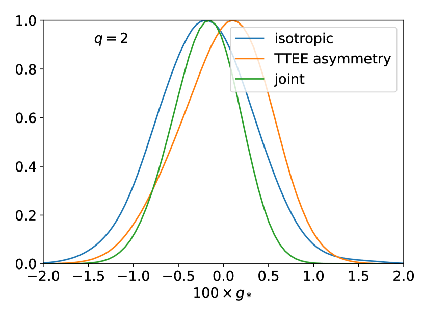
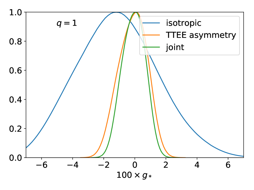
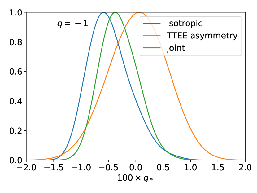
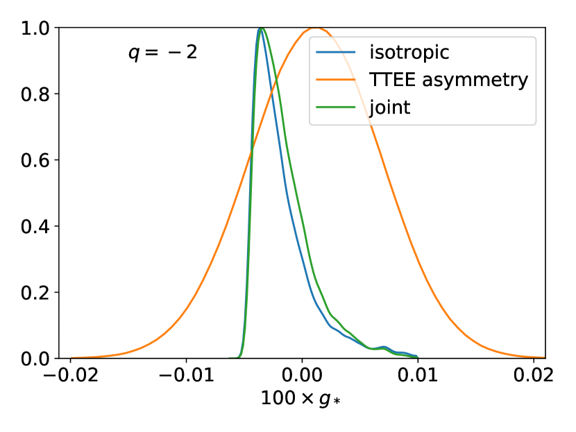
|
|||||||||||||||||||||||||||||||||||||||||||||||||||
|
|||||||||||||||||||||||||||||||||||||||||||||||||||
As in PCI15, we obtain constraints on the modulation parameters by forming quadratic maximum-likelihood estimates, , for the data and simulations. For this we use the component-separated data and 300 simulations provided by NILC, SEVEM, SMICA, and COMMANDER. For brevity we only show the SMICA results. We can then compute a covariance and likelihood as
where
| (119) |
We then evaluate the marginalized (over the angles) posterior for . For the isotropic constraints we simply include the modulation parameters in a CosmoMC run using Planck TT,TE,EE+lowE data, and then evaluate the marginalized (over all other CDM parameters) posterior for .
For the effect of on the isotropic spectra occurs mainly at high , and is highly degenerate with . This degeneracy leads to slightly less stringent constraints than what one would achieve with a fixed . We show the marginalized posteriors for this case in the top panels of Fig. 50, where we see that the isotropic constraints are roughly comparable in strength to (and fully consistent with) the constraints from the asymmetry data.
For the isotropic constraints are much more constraining than the modulation constraints, as seen in the bottom panels of Fig. 50. This is because for large scales the factor can become large and a negative will decrease isotropic power on those scales, which is compensated for by increasing and . Strongly negative values are disallowed by predicting unphysical negative power spectra at low . Note that even the parameter ranges in which the power spectra are reduced to close to zero are likely beyond the perturbative regime for the models in question, and so should be approached with caution. The isotropic constraints still prefer a slightly negative , likely due to being able to fit the power deficit at large scales. The joint constraint in this case is then greatly improved by the isotropic data.
Minimum- and values (relative to isotropic simulations) for are presented in Table 16. The addition of polarization does not affect the temperature results greatly.
Finally, when allowing the completely general form of quadrupolar modulation, i.e.,
| (120) |
with no restriction on the , we present results for the quantity in Table 17. In all cases there is no significant detection of quadrupolar modulation, as quantified by the values.
11 Conclusions
This paper summarizes the status of cosmic inflation in light of the Planck 2018 release. The main improvements are in the Planck polarization likelihoods. The 2018 release now includes a low- HFI polarization likelihood based on the 100- and 143-GHz channels. This likelihood is now the baseline, whereas the Planck 2015 likelihood was based only on the LFI 70-GHz channel data, which also have been updated in this release. Corrections for beam-leakage effects, which had been flagged in the 2015 release as the main limitation of the and data at that time, have improved the accuracy of the high- polarization likelihoods. Our analyses focus on the results obtained using the Planck baseline likelihoods alone, but results supplemented by the BK15 likelihood (when tensors are included) and a compilation of BAO likelihoods are also given in order to help break cosmological parameter degeneracies. We summarize the main results of this paper in the form of responses to a number of key questions.
-
1.
What is the value of the scalar tilt?
Using a characterization of polarization anisotropy better at all multipoles in this release, we find that at 68 % CL, including the full information provided by Planck (TT,TE,EE+lowE+lensing). The 2018 uncertainty is approximately 2/3 of that obtained with the Planck 2015 baseline likelihood. Importantly, this determination rules out perfect scale invariance (i.e., ) at . From an inflationary perspective, this result is consistent with slow-roll inflation evolving towards a natural exit.
-
2.
Does depend on the wavelength?
We investigated the possibility of a running spectral index, as well as a running of the running [i.e., the next two (subleading) terms in a power series expansion of in ], corresponding to non-negligible third- and fourth-order derivatives of the inflationary potential. Starting with its first 2013 cosmological release, Planck has removed any hint of a running spectral index, which had been suggested by pre-Planck data and would have pointed to inflationary models beyond the slow-roll approximation. Planck 2018 sets as the tightest 95 % CL constraint, when . No hints of further extensions, such as running of the running, are found with Planck 2018 data. These results are consistent with the simplest slow-roll dynamics for the inflaton. A detection of running at the level predicted by slow-roll models will require a combination of future ambitious CMB anisotropy experiments and galaxy surveys.
-
3.
Is the Universe spatially flat?
Most simple models of inflation predict a spatially flat universe, although inflationary models with a minimum degree of fine tuning producing a hyperbolic universe have been constructed. Planck has been the first experiment to constrain the spatial curvature at the percent level without any external information, thanks to the CMB lensing likelihood. Although negative values of provide a non-statistically significant improvement to the fit of Planck temperature and polarization data (compared to the minimal CDM model), Planck 2018 data including lensing constrain at 95 % CL. Combining with BAO data further tightens the uncertainty, constraining to lie within 0.4 % of a flat spatial geometry (at CL).
-
4.
Are tensor modes required?
Inflationary models predict that tensor modes were also excited during the nearly exponential expansion, with a power spectrum amplitude proportional to the energy scale of inflation. Using the measurement of CMB temperature and -mode polarization anisotropies from the quadrupole into the acoustic peak region, Planck has reduced the degeneracy between the tensor-to-scalar ratio and establishing the bound at 95 % CL, assuming as predicted by the simplest inflationary models. When the Planck likelihood is combined with the -mode polarization likelihood of the BICEP2-Keck Array experiment, a tight 95 % CL upper limit of is obtained, corresponding to a 95 % CL bound on the energy scale of inflation of . Planck 2018 and BK15 data also set tight bounds on gravitational waves generated in the early Universe when and are varied independently, complementary to the results obtained by the direct-detection interferometers LIGO and VIRGO at much higher frequencies.
-
5.
Which inflationary models are best able to account for the data?
Starting with the 2013 release using only a part of the data, Planck has substantially tightened the constraints on slow-roll inflationary models, ruling out hybrid models with and power-law inflation (PCI13). In combination with the BK15 data, Planck 2018 now strongly disfavours monomial models with and , natural inflation, and low-scale SUSY models. Within the representative cases studied in this paper, inflationary models such as , T and E -attractor models, D-brane inflation, and those having a potential with exponential tails provide good fits to Planck and BK15 data. We used two methods to reconstruct the inflaton potential beyond the slow-roll approximation: by Taylor expanding the inflaton potential or Hubble parameter in the observable region; and through a free-form reconstruction of the potential with cubic splines. No statistically significant detection beyond the second derivative of the potential was found, suggesting that the slow-roll approximation is adequate for the Planck 2018 likelihood in combination with the BK15 data.
-
6.
What model-independent constraints can be placed on the primordial power spectrum?
We reported on three different methods for the non-parametric reconstruction of the primordial power spectrum (penalized likelihood, a Bayesian spline reconstruction. and a method based on cubic splines). All three methods give broadly consistent results. In no case is any statistically significant evidence for a deviation from a pure power law found. The constraints on the deviations are at the few-percent level for wavenumbers in the range Mpc-1 probed by the CMB, the precise constraint depending on the level of smoothing allowed.
-
7.
Is there evidence for features in the primordial power spectrum?
We explored several classes of theoretically motivated parametric models with strong departures from a power law for the primordial power spectra and tested their predictions using combinations of Planck temperature and polarization power spectra. We also carried out an analysis using bispectrum data as well. No statistically significant evidence for features was found.
-
8.
Were the primordial cosmological perturbations solely adiabatic?
A key question is whether the primordial cosmological fluctuations consisted exclusively of adiabatic growing-mode perturbations or whether isocurvature perturbations, possibly correlated with the adiabatic mode and with each other, were also excited. The new polarization data has helped to sharpen constraints on the allowed isocurvature fraction compared to the Planck 2015 results. In correlated mixed adiabatic and isocurvature models, the 95 % CL upper bound for the non-adiabatic contribution to the observed CMB temperature variance is 1.3 %, 1.7 %, and 1.7 % for CDM, neutrino density, and neutrino velocity isocurvature, respectively. For this release we also report constraints on a scale-invariant compensated baryon-CDM isocurvature mode, which is uncorrelated with the adiabatic mode. This mode would cause an additional lensing-like smoothing at high and modify the lensing potential at . By using the temperature, polarization, and lensing data, we obtain the constraint at 68 % CL for the variance of the baryon isocurvature density perturbation. A detection of isocurvature modes would suggest the need for a theory beyond single-field inflation, which is able to excite only one mode.
-
9.
Were the primordial fluctuations statistically isotropic?
The Planck analysis has confirmed evidence at low statistical significance of anomalies in the CMB temperature anisotropies on large angular scales that are not alleviated in models with nontrivial topology or an anisotropic expansion (Planck Collaboration XVIII 2016). This motivates an exploration of inflation-based models giving such violation of statistical isotropy. We have found no statistically significant evidence in favour of a curvaton model for dipolar asymmetry (compared to the base-CDM model), nor any evidence for a quadrupolar asymmetry in the temperature or polarization anistropies. Theoretical models producing the observed temperature dipolar asymmetry make a prediction for the polarization dipolar asymmetry. We tested whether the fit to the temperature dipolar asymmetry gives a prediction for the polarization asymmetry consistent with the data. We found no statistically significant evidence that the pattern seen in temperature is repeated in polarization. However, the discriminating power of this test is weak, due to the low polarization signal-to-noise ratio on large angular scales.
The Planck 2013, 2015, and 2018 releases have substantially improved the constraints on the space of inflationary models, as described above. Future CMB polarization data will be crucial for further constraining those inflationary models that currently provide an adequate fit to Planck and other data. Forthcoming -mode polarization data will be decisive for determining whether the intriguing features in the temperature power spectrum, such as the deficit at –30, the smaller average amplitude at , and other anomalies at higher multipoles require new physics or whether these features are simply the result of statistical fluctuations plus instrumental noise. Improved measurements of the modes promise to constrain inflation even more tightly and it will be interesting to see how the search for modes evolves. One possibility would be a convincing detection of inflationary gravitational waves, but a tighter upper limit of is also an achievable outcome. Either case would substantially advance our understanding of inflation and the constraints on the physics of the very early Universe.
Acknowledgements.
We are grateful to Jan Hamann and Jim Zibin for extensive help with the final editing of this manuscript. The Planck Collaboration acknowledges the support of: ESA; CNES and CNRS/INSU-IN2P3-INP (France); ASI, CNR, and INAF (Italy); NASA and DoE (USA); STFC and UKSA (UK); CSIC, MINECO, JA, and RES (Spain); Tekes, AoF, and CSC (Finland); DLR and MPG (Germany); CSA (Canada); DTU Space (Denmark); SER/SSO (Switzerland); RCN (Norway); SFI (Ireland); FCT/MCTES (Portugal); ERC and PRACE (EU). A description of the Planck Collaboration and a list of its members, indicating which technical or scientific activities they have been involved in, can be found at http://www.cosmos.esa.int/web/planck/planck-collaboration.References
- Abazajian et al. (2016) Abazajian, K. N. et al., CMB-S4 Science Book, First Edition. 2016, 1610.02743
- Abbott et al. (2017) Abbott, B. P. et al., Upper Limits on the Stochastic Gravitational-Wave Background from Advanced LIGO’s First Observing Run. 2017, Phys. Rev. Lett., 118, 121101, [Erratum: Phys. Rev. Lett.119 (2017) 029901], 1612.02029
- Achucarro et al. (2014) Achucarro, A., Atal, V., Hu, B., Ortiz, P., & Torrado, J., Inflation with moderately sharp features in the speed of sound: Generalized slow roll and in-in formalism for power spectrum and bispectrum. 2014, Phys. Rev., D90, 023511, 1404.7522
- Achúcarro et al. (2014) Achúcarro, A., Atal, V., Ortiz, P., & Torrado, J., Localized correlated features in the CMB power spectrum and primordial bispectrum from a transient reduction in the speed of sound. 2014, Phys. Rev., D89, 103006, 1311.2552
- Achúcarro et al. (2011) Achúcarro, A., Gong, J.-O., Hardeman, S., Palma, G. A., & Patil, S. P., Features of heavy physics in the CMB power spectrum. 2011, JCAP, 1101, 030, 1010.3693
- Ackerman et al. (2007) Ackerman, L., Carroll, S. M., & Wise, M. B., Imprints of a Primordial Preferred Direction on the Microwave Background. 2007, Phys. Rev., D75, 083502, astro-ph/0701357
- Adams et al. (1993) Adams, F. C., Bond, J. R., Freese, K., Frieman, J. A., & Olinto, A. V., Natural inflation: Particle physics models, power law spectra for large scale structure, and constraints from COBE. 1993, Phys. Rev., D47, 426, hep-ph/9207245
- Adams et al. (2001) Adams, J. A., Cresswell, B., & Easther, R., Inflationary perturbations from a potential with a step. 2001, Phys. Rev., D64, 123514, astro-ph/0102236
- Addison et al. (2018) Addison, G. E., Watts, D. J., Bennett, C. L., et al., Elucidating CDM: Impact of Baryon Acoustic Oscillation Measurements on the Hubble Constant Discrepancy. 2018, Astrophys. J., 853, 119, 1707.06547
- Ade et al. (2016) Ade, P. A. R. et al., Improved Constraints on Cosmology and Foregrounds from BICEP2 and Keck Array Cosmic Microwave Background Data with Inclusion of 95 GHz Band. 2016, Phys. Rev. Lett., 116, 031302, 1510.09217
- Ade et al. (2018) Ade, P. A. R. et al., BICEP2 / Keck Array X: Constraints on Primordial Gravitational Waves using Planck, WMAP, and New BICEP2/Keck Observations through the 2015 Season. 2018, Phys. Rev. Lett., 121, 221301, 1810.05216
- Adshead et al. (2012) Adshead, P., Dvorkin, C., Hu, W., & Lim, E. A., Non-Gaussianity from Step Features in the Inflationary Potential. 2012, Phys. Rev., D85, 023531, 1110.3050
- Adshead & Hu (2014) Adshead, P. & Hu, W., Bounds on nonadiabatic evolution in single-field inflation. 2014, Phys. Rev., D89, 083531, 1402.1677
- Alam et al. (2016) Alam, S. et al., The clustering of galaxies in the completed SDSS-III Baryon Oscillation Spectroscopic Survey: cosmological analysis of the DR12 galaxy sample. 2016, Submitted to: Mon. Not. Roy. Astron. Soc., 1607.03155
- Albrecht & Steinhardt (1982) Albrecht, A. & Steinhardt, P. J., Cosmology for Grand Unified Theories with Radiatively Induced Symmetry Breaking. 1982, Phys. Rev. Lett., 48, 1220
- Amendola et al. (2002) Amendola, L., Gordon, C., Wands, D., & Sasaki, M., Correlated perturbations from inflation and the cosmic microwave background. 2002, Phys. Rev. Lett., 88, 211302, astro-ph/0107089
- Audren et al. (2013) Audren, B., Lesgourgues, J., Benabed, K., & Prunet, S., Conservative constraints on early cosmology: An illustration of the Monte Python cosmological parameter inference code. 2013, JCAP, 1302, 001, 1210.7183
- Bardeen et al. (1983) Bardeen, J. M., Steinhardt, P. J., & Turner, M. S., Spontaneous Creation of Almost Scale - Free Density Perturbations in an Inflationary Universe. 1983, Phys. Rev., D28, 679
- Bartolo et al. (2013) Bartolo, N., Cannone, D., & Matarrese, S., The Effective Field Theory of Inflation Models with Sharp Features. 2013, JCAP, 1310, 038, 1307.3483
- Bartolo & Liddle (2002) Bartolo, N. & Liddle, A. R., The Simplest curvaton model. 2002, Phys. Rev., D65, 121301, astro-ph/0203076
- Bartolo et al. (2001) Bartolo, N., Matarrese, S., & Riotto, A., Adiabatic and isocurvature perturbations from inflation: Power spectra and consistency relations. 2001, Phys. Rev., D64, 123504, astro-ph/0107502
- Bartolo et al. (2004a) Bartolo, N., Matarrese, S., & Riotto, A., Gauge-invariant temperature anisotropies and primordial non-Gaussianity. 2004a, Phys. Rev. Lett., 93, 231301, astro-ph/0407505
- Bartolo et al. (2004b) Bartolo, N., Matarrese, S., & Riotto, A., On non-Gaussianity in the curvaton scenario. 2004b, Phys. Rev., D69, 043503, hep-ph/0309033
- Bastero-Gil et al. (2016) Bastero-Gil, M., Berera, A., Ramos, R. O., & Rosa, J. G., Warm Little Inflaton. 2016, Phys. Rev. Lett., 117, 151301, 1604.08838
- Bean et al. (2006) Bean, R., Dunkley, J., & Pierpaoli, E., Constraining Isocurvature Initial Conditions with WMAP 3-year data. 2006, Phys. Rev., D74, 063503, astro-ph/0606685
- Behbahani et al. (2012) Behbahani, S. R., Dymarsky, A., Mirbabayi, M., & Senatore, L., (Small) Resonant non-Gaussianities: Signatures of a Discrete Shift Symmetry in the Effective Field Theory of Inflation. 2012, JCAP, 1212, 036, 1111.3373
- Behbahani & Green (2012) Behbahani, S. R. & Green, D., Collective Symmetry Breaking and Resonant Non-Gaussianity. 2012, JCAP, 1211, 056, 1207.2779
- Beltran et al. (2004) Beltran, M., García-Bellido, J., Lesgourgues, J., & Riazuelo, A., Bounds on CDM and neutrino isocurvature perturbations from CMB and LSS data. 2004, Phys. Rev., D70, 103530, astro-ph/0409326
- Beltrán et al. (2005) Beltrán, M., García-Bellido, J., Lesgourgues, J., & Viel, M., Squeezing the window on isocurvature modes with the Lyman- forest. 2005, Phys. Rev., D72, 103515, astro-ph/0509209
- Benetti (2013) Benetti, M., Updating constraints on inflationary features in the primordial power spectrum with the Planck data. 2013, Phys. Rev., D88, 087302, 1308.6406
- Bennett et al. (2012) Bennett, C., Larson, D., Weiland, J., et al., Nine-Year Wilkinson Microwave Anisotropy Probe (WMAP) Observations: Final Maps and Results. 2012, 1212.5225
- Bennett et al. (2011) Bennett, C. L., Hill, R. S., Hinshaw, G., et al., Seven-year Wilkinson Microwave Anisotropy Probe (WMAP) Observations: Are There Cosmic Microwave Background Anomalies? 2011, ApJS, 192, 17, 1001.4758
- Bennett et al. (2013) Bennett, C. L., Larson, D., Weiland, J. L., et al., Nine-year Wilkinson Microwave Anisotropy Probe (WMAP) Observations: Final Maps and Results. 2013, ApJS, 208, 20, 1212.5225
- Berera (1995) Berera, A., Warm inflation. 1995, Phys. Rev. Lett., 75, 3218, astro-ph/9509049
- Beutler et al. (2011) Beutler, F., Blake, C., Colless, M., et al., The 6dF Galaxy Survey: Baryon Acoustic Oscillations and the Local Hubble Constant. 2011, MNRAS, 416, 3017, 1106.3366
- Bezrukov & Shaposhnikov (2008) Bezrukov, F. & Shaposhnikov, M., The Standard Model Higgs boson as the inflaton. 2008, Phys. Lett., B659, 703
- Bezrukov & Gorbunov (2012) Bezrukov, F. L. & Gorbunov, D. S., Distinguishing between R2-inflation and Higgs-inflation. 2012, Phys. Lett., B713, 365, 1111.4397
- BICEP2/Keck Array and Planck Collaborations (2015) BICEP2/Keck Array and Planck Collaborations, Joint Analysis of BICEP2/Keck Array and Planck Data. 2015, Phys. Rev. Lett., 114, 101301, 1502.00612
- Blas et al. (2011) Blas, D., Lesgourgues, J., & Tram, T., The Cosmic Linear Anisotropy Solving System (CLASS) II: Approximation schemes. 2011, JCAP, 1107, 034, 1104.2933
- Boubekeur & Lyth (2005) Boubekeur, L. & Lyth, D., Hilltop inflation. 2005, JCAP, 0507, 010, hep-ph/0502047
- Boyle et al. (2004) Boyle, L. A., Steinhardt, P. J., & Turok, N., The Cosmic gravitational wave background in a cyclic universe. 2004, Phys. Rev., D69, 127302, hep-th/0307170
- Bozza et al. (2003) Bozza, V., Giovannini, M., & Veneziano, G., Cosmological perturbations from a new physics hypersurface. 2003, JCAP, 0305, 001, hep-th/0302184
- Brandenberger et al. (2007) Brandenberger, R. H., Nayeri, A., Patil, S. P., & Vafa, C., Tensor Modes from a Primordial Hagedorn Phase of String Cosmology. 2007, Phys. Rev. Lett., 98, 231302, hep-th/0604126
- Brout et al. (1978) Brout, R., Englert, F., & Gunzig, E., The Creation of the Universe as a Quantum Phenomenon. 1978, Annals Phys., 115, 78
- Bucher et al. (2004) Bucher, M., Dunkley, J., Ferreira, P., Moodley, K., & Skordis, C., The Initial conditions of the universe: How much isocurvature is allowed? 2004, Phys. Rev. Lett., 93, 081301, astro-ph/0401417
- Bucher et al. (1995) Bucher, M., Goldhaber, A. S., & Turok, N., An open universe from inflation. 1995, Phys. Rev., D52, 3314, hep-ph/9411206
- Bucher et al. (2000) Bucher, M., Moodley, K., & Turok, N., The General primordial cosmic perturbation. 2000, Phys. Rev., D62, 083508, astro-ph/9904231
- Burgess et al. (2002) Burgess, C., Martineau, P., Quevedo, F., Rajesh, G., & Zhang, R., Brane - anti-brane inflation in orbifold and orientifold models. 2002, JHEP, 0203, 052, hep-th/0111025
- Burgess et al. (2013) Burgess, C. P., Cicoli, M., & Quevedo, F., String Inflation After Planck 2013. 2013, JCAP, 1311, 003, 1306.3512
- Byrnes et al. (2016a) Byrnes, C. T., Regan, D., Seery, D., & Tarrant, E. R. M., Implications of the cosmic microwave background power asymmetry for the early universe. 2016a, Phys. Rev., D93, 123003, 1601.01970
- Byrnes et al. (2016b) Byrnes, C. T., Regan, D., Seery, D., & Tarrant, E. R. M., The hemispherical asymmetry from a scale-dependent inflationary bispectrum. 2016b, JCAP, 1606, 025, 1511.03129
- Byrnes & Wands (2006) Byrnes, C. T. & Wands, D., Curvature and isocurvature perturbations from two-field inflation in a slow-roll expansion. 2006, Phys. Rev., D74, 043529, astro-ph/0605679
- Cabass et al. (2016) Cabass, G., Pagano, L., Salvati, L., et al., Updated Constraints and Forecasts on Primordial Tensor Modes. 2016, Phys. Rev., D93, 063508, 1511.05146
- Calabrese et al. (2008) Calabrese, E., Slosar, A., Melchiorri, A., Smoot, G. F., & Zahn, O., Cosmic Microwave Weak lensing data as a test for the dark universe. 2008, Phys. Rev. D, 77, 123531, 0803.2309
- Chen (2010) Chen, X., Primordial Non-Gaussianities from Inflation Models. 2010, Advances in Astronomy, 2010, 1002.1416
- Chen (2012) Chen, X., Primordial Features as Evidence for Inflation. 2012, JCAP, 1201, 038, 1104.1323
- Chen et al. (2007) Chen, X., Easther, R., & Lim, E. A., Large Non-Gaussianities in Single Field Inflation. 2007, JCAP, 0706, 023, astro-ph/0611645
- Chen et al. (2008) Chen, X., Easther, R., & Lim, E. A., Generation and Characterization of Large Non-Gaussianities in Single Field Inflation. 2008, JCAP, 0804, 010, 0801.3295
- Chluba et al. (2015) Chluba, J., Hamann, J., & Patil, S. P., Features and New Physical Scales in Primordial Observables: Theory and Observation. 2015, Int. J. Mod. Phys., D24, 1530023, 1505.01834
- Chung & Upadhye (2017) Chung, D. J. H. & Upadhye, A., A Hint of a Blue Axion Isocurvature Spectrum? 2017, 1711.06736
- Cicoli et al. (2009) Cicoli, M., Burgess, C., & Quevedo, F., Fibre Inflation: Observable Gravity Waves from IIB String Compactifications. 2009, JCAP, 0903, 013, 0808.0691
- Cline et al. (2003) Cline, J. M., Crotty, P., & Lesgourgues, J., Does the small CMB quadrupole moment suggest new physics? 2003, JCAP, 0309, 010, astro-ph/0304558
- Contaldi et al. (2003) Contaldi, C. R., Peloso, M., Kofman, L., & Linde, A. D., Suppressing the lower multipoles in the CMB anisotropies. 2003, JCAP, 0307, 002, astro-ph/0303636
- Contreras et al. (2018) Contreras, D., Hutchinson, J., Moss, A., Scott, D., & Zibin, J. P., Closing in on the large-scale CMB power asymmetry. 2018, Phys. Rev., D97, 063504, 1709.10134
- Contreras et al. (2017) Contreras, D., Zibin, J. P., Scott, D., Banday, A. J., & Górski, K. M., Testing physical models for dipolar asymmetry with CMB polarization. 2017, Phys. Rev., D96, 123522, 1704.03143
- Danielsson (2002) Danielsson, U. H., A Note on inflation and trans-Planckian physics. 2002, Phys. Rev., D66, 023511, hep-th/0203198
- Dunkley et al. (2005) Dunkley, J., Bucher, M., Ferreira, P., Moodley, K., & Skordis, C., Measuring the geometry of the Universe in the presence of isocurvature modes. 2005, Phys. Rev. Lett., 95, 261303, astro-ph/0507473
- Durakovic et al. (2018) Durakovic, A., Hunt, P., Mukherjee, S., Sarkar, S., & Souradeep, T., Reconstruction of a direction-dependent primordial power spectrum from Planck CMB data. 2018, JCAP, 1802, 012, 1711.08441
- Dvali et al. (2001) Dvali, G., Shafi, Q., & Solganik, S., D-brane inflation. 2001, hep-th/0105203
- Dvali & Tye (1999) Dvali, G. & Tye, S. H., Brane inflation. 1999, Phys. Lett., B450, 72, hep-ph/9812483
- Dvali et al. (1994) Dvali, G. R., Shafi, Q., & Schaefer, R. K., Large scale structure and supersymmetric inflation without fine tuning. 1994, Phys. Rev. Lett., 73, 1886, hep-ph/9406319
- Easther & Flauger (2014) Easther, R. & Flauger, R., Planck Constraints on Monodromy Inflation. 2014, JCAP, 1402, 037, 1308.3736
- Easther et al. (2005) Easther, R., Kinney, W. H., & Peiris, H., Observing trans-Planckian signatures in the cosmic microwave background. 2005, JCAP, 0505, 009, astro-ph/0412613
- Efstathiou & Bond (1986) Efstathiou, G. & Bond, J. R., Isocurvature cold dark matter fluctuations. 1986, MNRAS, 218, 103
- Efstathiou & Bond (1987) Efstathiou, G. & Bond, J. R., Microwave anisotropy constraints on isocurvature baryon models. 1987, MNRAS, 227, 33P
- Efstathiou & Bond (1999) Efstathiou, G. & Bond, J. R., Cosmic confusion: Degeneracies among cosmological parameters derived from measurements of microwave background anisotropies. 1999, Mon. Not. Roy. Astron. Soc., 304, 75, astro-ph/9807103
- Enqvist et al. (2000) Enqvist, K., Kurki-Suonio, H., & Valiviita, J., Limits on isocurvature fluctuations from boomerang and MAXIMA. 2000, Phys. Rev., D62, 103003, astro-ph/0006429
- Enqvist et al. (2002) Enqvist, K., Kurki-Suonio, H., & Valiviita, J., Open and closed CDM isocurvature models contrasted with the CMB data. 2002, Phys. Rev., D65, 043002, astro-ph/0108422
- Enqvist & Sloth (2002) Enqvist, K. & Sloth, M. S., Adiabatic CMB perturbations in pre-big bang string cosmology. 2002, Nucl. Phys., B626, 395, hep-ph/0109214
- Erickcek et al. (2009) Erickcek, A. L., Hirata, C. M., & Kamionkowski, M., A Scale-Dependent Power Asymmetry from Isocurvature Perturbations. 2009, Phys. Rev., D80, 083507, 0907.0705
- Eriksen et al. (2004) Eriksen, H. K., Hansen, F. K., Banday, A. J., Górski, K. M., & Lilje, P. B., Asymmetries in the Cosmic Microwave Background anisotropy field. 2004, Astrophys. J., 605, 14, [Erratum: Astrophys. J.609,1198(2004)], astro-ph/0307507
- Fakir & Unruh (1990) Fakir, R. & Unruh, W., Improvement on cosmological chaotic inflation through nonminimal coupling. 1990, Phys. Rev., D41, 1783
- Fergusson et al. (2015) Fergusson, J. R., Gruetjen, H. F., Shellard, E. P. S., & Liguori, M., Combining power spectrum and bispectrum measurements to detect oscillatory features. 2015, Phys. Rev., D91, 023502, 1410.5114
- Fergusson et al. (2015) Fergusson, J. R., Gruetjen, H. F., Shellard, E. P. S., & Wallisch, B., Polyspectra searches for sharp oscillatory features in cosmic microwave sky data. 2015, Phys. Rev. D, 91, 123506, 1412.6152
- Fergusson et al. (2010) Fergusson, J. R., Liguori, M., & Shellard, E. P. S., General CMB and primordial bispectrum estimation: Mode expansion, map making, and measures of FNL. 2010, Phys. Rev. D, 82, 023502, 0912.5516
- Fergusson et al. (2012) Fergusson, J. R., Liguori, M., & Shellard, E. P. S., The CMB bispectrum. 2012, J. Cosmology Astropart. Phys., 12, 032, 1006.1642
- Fergusson & Shellard (2009) Fergusson, J. R. & Shellard, E. P. S., The shape of primordial non-Gaussianity and the CMB bispectrum. 2009, Phys. Rev., D80, 043510, 0812.3413
- Feroz et al. (2009) Feroz, F., Hobson, M., & Bridges, M., MultiNest: an efficient and robust Bayesian inference tool for cosmology and particle physics. 2009, MNRAS, 398, 1601, 0809.3437
- Feroz et al. (2013) Feroz, F., Hobson, M., Cameron, E., & Pettitt, A., Importance Nested Sampling and the MultiNest Algorithm. 2013, 1306.2144
- Ferrara & Kallosh (2016) Ferrara, S. & Kallosh, R., Seven-disk manifold, -attractors, and modes. 2016, Phys. Rev., D94, 126015, 1610.04163
- Ferrara et al. (2013) Ferrara, S., Kallosh, R., Linde, A., & Porrati, M., Minimal Supergravity Models of Inflation. 2013, Phys. Rev., D88, 085038, 1307.7696
- Finelli et al. (2010) Finelli, F., Hamann, J., Leach, S. M., & Lesgourgues, J., Single-field inflation constraints from CMB and SDSS data. 2010, JCAP, 1004, 011, 0912.0522
- Finelli et al. (2018) Finelli, F. et al., Exploring cosmic origins with CORE: Inflation. 2018, JCAP, 1804, 016, 1612.08270
- Flauger et al. (2010) Flauger, R., McAllister, L., Pajer, E., Westphal, A., & Xu, G., Oscillations in the CMB from Axion Monodromy Inflation. 2010, JCAP, 1006, 009, 0907.2916
- Flauger et al. (2010) Flauger, R., McAllister, L., Pajer, E., Westphal, A., & Xu, G., Oscillations in the CMB from axion monodromy inflation. 2010, JCAP, 6, 9, 0907.2916
- Flauger et al. (2017a) Flauger, R., McAllister, L., Silverstein, E., & Westphal, A., Drifting Oscillations in Axion Monodromy. 2017a, JCAP, 1710, 055, 1412.1814
- Flauger et al. (2017b) Flauger, R., Mirbabayi, M., Senatore, L., & Silverstein, E., Productive Interactions: Heavy particles and non-Gaussianity. 2017b, JCAP, 1710, 058, 1606.00513
- Flauger & Pajer (2011) Flauger, R. & Pajer, E., Resonant Non-Gaussianity. 2011, JCAP, 1101, 017, 1002.0833
- Freese et al. (1990) Freese, K., Frieman, J. A., & Olinto, A. V., Natural inflation with pseudo Nambu-Goldstone bosons. 1990, Phys. Rev. Lett., 65, 3233
- Garcia-Bellido et al. (2009) Garcia-Bellido, J., Figueroa, D. G., & Rubio, J., Preheating in the Standard Model with the Higgs-Inflaton coupled to gravity. 2009, Phys. Rev., D79, 063531, 0812.4624
- García-Bellido et al. (2002) García-Bellido, J., Rabadan, R., & Zamora, F., Inflationary scenarios from branes at angles. 2002, JHEP, 0201, 036, hep-th/0112147
- García-Bellido & Wands (1996) García-Bellido, J. & Wands, D., Metric perturbations in two-field inflation. 1996, Phys. Rev., D53, 5437, astro-ph/9511029
- Garriga & Mukhanov (1999) Garriga, J. & Mukhanov, V. F., Perturbations in -inflation. 1999, Physics Letters B, 458, 219, arXiv:hep-th/9904176
- Gasperini & Veneziano (1993) Gasperini, M. & Veneziano, G., Pre - big bang in string cosmology. 1993, Astropart. Phys., 1, 317, hep-th/9211021
- Gauthier & Bucher (2012) Gauthier, C. & Bucher, M., Reconstructing the primordial power spectrum from the CMB. 2012, JCAP, 1210, 050, astro-ph/1209.2147
- Goncharov & Linde (1984) Goncharov, A. & Linde, A. D., Chaotic Inflation of the Universe in Supergravity. 1984, Sov. Phys. JETP, 59, 930
- Gong & Stewart (2001) Gong, J.-O. & Stewart, E. D., The density perturbation power spectrum to second order corrections in the slow roll expansion. 2001, Phys. Lett., B510, 1, astro-ph/0101225
- Gong & Yamaguchi (2017) Gong, J.-O. & Yamaguchi, M., Correlated primordial spectra in effective theory of inflation. 2017, Phys. Rev., D95, 083510, 1701.05875
- Gordon & Lewis (2003) Gordon, C. & Lewis, A., Observational constraints on the curvaton model of inflation. 2003, Phys. Rev., D67, 123513, astro-ph/0212248
- Gordon & Pritchard (2009) Gordon, C. & Pritchard, J. R., Forecasted 21 cm constraints on compensated isocurvature perturbations. 2009, Phys. Rev., D80, 063535, 0907.5400
- Gordon et al. (2001) Gordon, C., Wands, D., Bassett, B. A., & Maartens, R., Adiabatic and entropy perturbations from inflation. 2001, Phys. Rev., D63, 023506, astro-ph/0009131
- Gott (1982) Gott, J., Creation of Open Universes from de Sitter Space. 1982, Nature, 295, 304
- Gott & Statler (1984) Gott, J. & Statler, T., Constraints on the formation of bubble universes. 1984, Phys. Lett., B136, 157
- Graham et al. (1994) Graham, R. L., Knuth, D. E., & Patashnik, O. 1994, Concrete Mathematics: A Foundation for Computer Science, 2nd edn. (Boston, MA, USA: Addison-Wesley Longman Publishing Co., Inc.)
- Grin et al. (2011a) Grin, D., Dore, O., & Kamionkowski, M., Compensated Isocurvature Perturbations and the Cosmic Microwave Background. 2011a, Phys. Rev., D84, 123003, 1107.5047
- Grin et al. (2011b) Grin, D., Dore, O., & Kamionkowski, M., Do baryons trace dark matter in the early universe? 2011b, Phys. Rev. Lett., 107, 261301, 1107.1716
- Grin et al. (2014) Grin, D., Hanson, D., Holder, G. P., Doré, O., & Kamionkowski, M., Baryons do trace dark matter 380,000 years after the big bang: Search for compensated isocurvature perturbations with WMAP 9-year data. 2014, Phys. Rev., D89, 023006, 1306.4319
- Gruppuso et al. (2016) Gruppuso, A., Kitazawa, N., Mandolesi, N., Natoli, P., & Sagnotti, A., Pre-Inflationary Relics in the CMB? 2016, Phys. Dark Univ., 11, 68, 1508.00411
- Guth (1981) Guth, A. H., The Inflationary Universe: A Possible Solution to the Horizon and Flatness Problems. 1981, Phys. Rev., D23, 347
- Guth et al. (2014) Guth, A. H., Kaiser, D. I., & Nomura, Y., Inflationary paradigm after Planck 2013. 2014, Phys. Lett., B733, 112, 1312.7619
- Guth & Pi (1982) Guth, A. H. & Pi, S., Fluctuations in the New Inflationary Universe. 1982, Phys. Rev. Lett., 49, 1110
- Haga et al. (2018) Haga, T., Inomata, K., Ota, A., & Ravenni, A., Exploring compensated isocurvature perturbations with CMB spectral distortion anisotropies. 2018, 1805.08773
- Hamann et al. (2010) Hamann, J., Shafieloo, A., & Souradeep, T., Features in the primordial power spectrum? A frequentist analysis. 2010, JCAP, 1004, 010, 0912.2728
- Handley (2018) Handley, W., fgivenx: Functional Posterior Plotter. 2018, The Journal of Open Source Software, 3
- Handley et al. (2019) Handley, W., Lasenby, A., Peiris, H., & Hobson, M., Bayesian inflationary reconstructions from Planck 2018 data. 2019, Phys. Rev. D, in preparation
- Handley et al. (2015a) Handley, W. J., Hobson, M. P., & Lasenby, A. N., POLYCHORD: nested sampling for cosmology. 2015a, MNRAS, 450, L61, 1502.01856
- Handley et al. (2015b) Handley, W. J., Hobson, M. P., & Lasenby, A. N., POLYCHORD: next-generation nested sampling. 2015b, MNRAS, 453, 4384, 1506.00171
- Harrison (1970) Harrison, E. R., Fluctuations at the threshold of classical cosmology. 1970, Phys. Rev., D1, 2726
- Haslam et al. (1982) Haslam, C. G. T., Salter, C. J., Stoffel, H., & Wilson, W. E., A 408 MHz all-sky continuum survey. II - The atlas of contour maps. 1982, A&AS, 47, 1
- Hawking (1982) Hawking, S., The Development of Irregularities in a Single Bubble Inflationary Universe. 1982, Phys. Lett., B115, 295
- Hazra et al. (2014a) Hazra, D. K., Shafieloo, A., Smoot, G. F., & Starobinsky, A. A., Inflation with Whip-Shaped Suppressed Scalar Power Spectra. 2014a, Phys. Rev. Lett., 113, 071301, 1404.0360
- Hazra et al. (2016) Hazra, D. K., Shafieloo, A., Smoot, G. F., & Starobinsky, A. A., Primordial features and Planck polarization. 2016, JCAP, 1609, 009, 1605.02106
- Hazra et al. (2014b) Hazra, D. K., Shafieloo, A., & Souradeep, T., Primordial power spectrum from Planck. 2014b, JCAP, 1411, 011, 1406.4827
- He et al. (2015) He, C., Grin, D., & Hu, W., Compensated isocurvature perturbations in the curvaton model. 2015, Phys. Rev., D92, 063018, 1505.00639
- Hee et al. (2016) Hee, S., Vázquez, J. A., Handley, W. J., Hobson, M. P., & Lasenby, A. N., Constraining the dark energy equation of state using Bayes theorem and the Kullback-Leibler divergence. 2016, ArXiv e-prints, 1607.00270
- Heinrich et al. (2016) Heinrich, C. H., Grin, D., & Hu, W., Lensing Bias to CMB Measurements of Compensated Isocurvature Perturbations. 2016, Phys. Rev., D94, 043534, 1605.08439
- Hivon et al. (2017) Hivon, E., Mottet, S., & Ponthieu, N., QuickPol: Fast calculation of effective beam matrices for CMB polarization. 2017, Astron. Astrophys., 598, A25, 1608.08833
- Holder et al. (2010) Holder, G. P., Nollett, K. M., & van Engelen, A., On Possible Variation in the Cosmological Baryon Fraction. 2010, Astrophys. J., 716, 907, 0907.3919
- Hou et al. (2014) Hou, Z. et al., Constraints on Cosmology from the Cosmic Microwave Background Power Spectrum of the 2500 deg2 SPT-SZ Survey. 2014, Astrophys. J., 782, 74, 1212.6267
- Hu (2011) Hu, W., Generalized Slow Roll for Non-Canonical Kinetic Terms. 2011, Phys. Rev., D84, 027303, 1104.4500
- Hunt & Sarkar (2014) Hunt, P. & Sarkar, S., Reconstruction of the primordial power spectrum of curvature perturbations using multiple data sets. 2014, JCAP, 1401, 025, 1308.2317
- Hunt & Sarkar (2015) Hunt, P. & Sarkar, S., Search for features in the spectrum of primordial perturbations using Planck and other datasets. 2015, JCAP, 1512, 052, 1510.03338
- Ijjas & Steinhardt (2016) Ijjas, A. & Steinhardt, P. J., Implications of Planck 2015 for inflationary, ekpyrotic and anamorphic bouncing cosmologies. 2016, Class. Quant. Grav., 33, 044001, 1512.09010
- Ijjas et al. (2013) Ijjas, A., Steinhardt, P. J., & Loeb, A., Inflationary paradigm in trouble after Planck2013. 2013, Phys. Lett., B723, 261, 1304.2785
- Jackson & Shiu (2013) Jackson, M. G. & Shiu, G., Study of the consistency relation for single-field inflation with power spectrum oscillations. 2013, Phys. Rev., D88, 123511, 1303.4973
- Jackson et al. (2014) Jackson, M. G., Wandelt, B., & Bouchet, F., Angular Correlation Functions for Models with Logarithmic Oscillations. 2014, Phys. Rev., D89, 023510, 1303.3499
- Jeffreys (1998) Jeffreys, H. 1998, Theory of Probability, 3rd edn. (Oxford University Press)
- Kachru et al. (2003) Kachru, S., Kallosh, R., Linde, A. D., et al., Towards inflation in string theory. 2003, JCAP, 0310, 013, hep-th/0308055
- Kallosh et al. (2013) Kallosh, R., Linde, A., & Roest, D., Superconformal Inflationary -Attractors. 2013, JHEP, 1311, 198, 1311.0472
- Kallosh et al. (2017) Kallosh, R., Linde, A., Wrase, T., & Yamada, Y., Maximal Supersymmetry and B-Mode Targets. 2017, JHEP, 04, 144, 1704.04829
- Kaloper et al. (2011) Kaloper, N., Lawrence, A., & Sorbo, L., An Ignoble Approach to Large Field Inflation. 2011, JCAP, 1103, 023, 1101.0026
- Kasuya & Kawasaki (2009) Kasuya, S. & Kawasaki, M., Axion isocurvature fluctuations with extremely blue spectrum. 2009, Phys. Rev., D80, 023516, 0904.3800
- Kazanas (1980) Kazanas, D., Dynamics of the Universe and Spontaneous Symmetry Breaking. 1980, Astrophys. J., 241, L59
- Keskitalo et al. (2007) Keskitalo, R., Kurki-Suonio, H., Muhonen, V., & Valiviita, J., Hints of Isocurvature Perturbations in the Cosmic Microwave Background. 2007, JCAP, 0709, 008, astro-ph/0611917
- Kleban & Schillo (2012) Kleban, M. & Schillo, M., Spatial Curvature Falsifies Eternal Inflation. 2012, JCAP, 1206, 029, 1202.5037
- Kobayashi et al. (2010) Kobayashi, T., Yamaguchi, M., & Yokoyama, J., G-inflation: Inflation driven by the Galileon field. 2010, Phys. Rev. Lett., 105, 231302, 1008.0603
- Komatsu et al. (2009) Komatsu, E. et al., Five-Year Wilkinson Microwave Anisotropy Probe (WMAP) Observations: Cosmological Interpretation. 2009, Astrophys. J. Suppl., 180, 330, 0803.0547
- Kuhnel & Schwarz (2010) Kuhnel, F. & Schwarz, D. J., Large-Scale Suppression from Stochastic Inflation. 2010, Phys. Rev. Lett., 105, 211302, 1003.3014
- Kurki-Suonio et al. (2005) Kurki-Suonio, H., Muhonen, V., & Valiviita, J., Correlated Primordial Perturbations in Light of CMB and LSS Data. 2005, Phys. Rev., D71, 063005, astro-ph/0412439
- Langlois (1999) Langlois, D., Correlated adiabatic and isocurvature perturbations from double inflation. 1999, Phys. Rev., D59, 123512, astro-ph/9906080
- Langlois & Riazuelo (2000) Langlois, D. & Riazuelo, A., Correlated mixtures of adiabatic and isocurvature cosmological perturbations. 2000, Phys. Rev., D62, 043504, astro-ph/9912497
- Leach et al. (2002) Leach, S. M., Liddle, A. R., Martin, J., & Schwarz, D. J., Cosmological parameter estimation and the inflationary cosmology. 2002, Phys. Rev., D66, 023515, astro-ph/0202094
- Lesgourgues (2011) Lesgourgues, J., The Cosmic Linear Anisotropy Solving System (CLASS) I: Overview. 2011, 1104.2932
- Lewis & Bridle (2002) Lewis, A. & Bridle, S., Cosmological parameters from CMB and other data: A Monte Carlo approach. 2002, Phys. Rev. D, 66, 103511, arXiv:astro-ph/0205436
- Lewis & Challinor (2006) Lewis, A. & Challinor, A., Weak gravitational lensing of the CMB. 2006, Phys. Rept., 429, 1, astro-ph/0601594
- Lewis et al. (2000) Lewis, A., Challinor, A., & Lasenby, A., Efficient Computation of CMB Anisotropies in Closed FRW Models. 2000, Astrophys. J., 538, 473, astro-ph/9911177
- Liddle & Leach (2003) Liddle, A. R. & Leach, S. M., How long before the end of inflation were observable perturbations produced? 2003, Phys. Rev., D68, 103503, astro-ph/0305263
- Linde (2015) Linde, A. 2015, in Proceedings, 100th Les Houches Summer School: Post-Planck Cosmology: Les Houches, France, July 8 - August 2, 2013, 231–316
- Linde (2017) Linde, A. 2017, in Black Holes, Gravitational Waves and Spacetime Singularities Rome, Italy, May 9-12, 2017
- Linde (1982) Linde, A. D., A New Inflationary Universe Scenario: A Possible Solution of the Horizon, Flatness, Homogeneity, Isotropy and Primordial Monopole Problems. 1982, Phys. Lett., B108, 389
- Linde (1983) Linde, A. D., Chaotic Inflation. 1983, Phys. Lett., B129, 177
- Linde (1985) Linde, A. D., Generation of Isothermal Density Perturbations in the Inflationary Universe. 1985, Phys. Lett., B158, 375
- Linde & Mukhanov (1997) Linde, A. D. & Mukhanov, V. F., Non-Gaussian isocurvature perturbations from inflation. 1997, Phys. Rev., D56, 535, astro-ph/9610219
- Lucchin et al. (1986) Lucchin, F., Matarrese, S., & Pollock, M. D., Inflation with a Non-minimally Coupled Scalar Field. 1986, Phys. Lett., 167B, 163
- Lyth & Stewart (1990) Lyth, D. H. & Stewart, E. D., Inflationary density perturbations with Omega 1. 1990, Phys. Lett., B252, 336
- Lyth et al. (2003) Lyth, D. H., Ungarelli, C., & Wands, D., The Primordial Density Perturbation in the Curvaton Scenario. 2003, Phys. Rev., D67, 023503, astro-ph/0208055
- Lyth & Wands (2002) Lyth, D. H. & Wands, D., Generating the curvature perturbation without an inflaton. 2002, Phys. Lett., B524, 5, hep-ph/0110002
- Maleknejad et al. (2013) Maleknejad, A., Sheikh-Jabbari, M. M., & Soda, J., Gauge Fields and Inflation. 2013, Phys. Rept., 528, 161, 1212.2921
- Marsh (2016) Marsh, D. J. E., Axion Cosmology. 2016, Phys. Rept., 643, 1, 1510.07633
- Martin & Brandenberger (2003) Martin, J. & Brandenberger, R., On the dependence of the spectra of fluctuations in inflationary cosmology on trans-Planckian physics. 2003, Phys. Rev., D68, 063513, hep-th/0305161
- Martin & Ringeval (2010) Martin, J. & Ringeval, C., First CMB Constraints on the Inflationary Reheating Temperature. 2010, Phys. Rev., D82, 023511, 1004.5525
- Martin et al. (2014a) Martin, J., Ringeval, C., Trotta, R., & Vennin, V., The Best Inflationary Models After Planck. 2014a, JCAP, 1403, 039, 1312.3529
- Martin et al. (2014b) Martin, J., Ringeval, C., & Vennin, V., Encyclopædia Inflationaris. 2014b, Phys. Dark Univ., 1303.3787
- McAllister et al. (2010) McAllister, L., Silverstein, E., & Westphal, A., Gravity Waves and Linear Inflation from Axion Monodromy. 2010, Phys. Rev., D82, 046003, 0808.0706
- McAllister et al. (2014) McAllister, L., Silverstein, E., Westphal, A., & Wrase, T., The Powers of Monodromy. 2014, JHEP, 09, 123, 1405.3652
- Meerburg (2014) Meerburg, P. D., Alleviating the tension at low through axion monodromy. 2014, Phys. Rev., D90, 063529, 1406.3243
- Meerburg et al. (2015) Meerburg, P. D., Hloçek, R., Hadzhiyska, B., & Meyers, J., Multiwavelength constraints on the inflationary consistency relation. 2015, Phys. Rev., D91, 103505, 1502.00302
- Meerburg & Münchmeyer (2015) Meerburg, P. D. & Münchmeyer, M., Optimal CMB estimators for bispectra from excited states. 2015, Phys. Rev., D92, 063527, 1505.05882
- Meerburg et al. (2016) Meerburg, P. D., Münchmeyer, M., & Wandelt, B., Joint resonant CMB power spectrum and bispectrum estimation. 2016, Phys. Rev., D93, 043536, 1510.01756
- Meerburg & Pajer (2013) Meerburg, P. D. & Pajer, E., Observational Constraints on Gauge Field Production in Axion Inflation. 2013, JCAP, 1302, 017, 1203.6076
- Meerburg et al. (2014a) Meerburg, P. D., Spergel, D. N., & Wandelt, B. D. 2014a, in Proceedings, 49th Rencontres de Moriond on Cosmology: La Thuile, Italy, March 15-22, 2014, 27–32
- Meerburg et al. (2014b) Meerburg, P. D., Spergel, D. N., & Wandelt, B. D., Searching for oscillations in the primordial power spectrum. I. Perturbative approach. 2014b, Phys. Rev., D89, 063536, 1308.3704
- Meerburg et al. (2014c) Meerburg, P. D., Spergel, D. N., & Wandelt, B. D., Searching for oscillations in the primordial power spectrum. II. Constraints from Planck data. 2014c, Phys. Rev., D89, 063537, 1308.3705
- Meerburg et al. (2009) Meerburg, P. D., van der Schaar, J. P., & Corasaniti, P. S., Signatures of Initial State Modifications on Bispectrum Statistics. 2009, JCAP, 0905, 018, 0901.4044
- Miranda & Hu (2014) Miranda, V. & Hu, W., Inflationary Steps in the Planck Data. 2014, Phys. Rev., D89, 083529, 1312.0946
- Miranda et al. (2012) Miranda, V., Hu, W., & Adshead, P., Warp Features in DBI Inflation. 2012, Phys. Rev., D86, 063529, 1207.2186
- Miranda et al. (2015) Miranda, V., Hu, W., & Dvorkin, C., Polarization Predictions for Inflationary CMB Power Spectrum Features. 2015, Phys. Rev., D91, 063514, 1411.5956
- Mollerach (1990) Mollerach, S., Isocurvature baryon perturbations and inflation. 1990, Phys. Rev., D42, 313
- Moodley et al. (2004) Moodley, K., Bucher, M., Dunkley, J., Ferreira, P., & Skordis, C., Constraints on isocurvature models from the WMAP first-year data. 2004, Phys. Rev., D70, 103520, astro-ph/0407304
- Mooij et al. (2016) Mooij, S., Palma, G. A., Panotopoulos, G., & Soto, A., Consistency relations for sharp inflationary non-Gaussian features. 2016, JCAP, 1609, 004, 1604.03533
- Moroi & Takahashi (2001) Moroi, T. & Takahashi, T., Effects of cosmological moduli fields on cosmic microwave background. 2001, Phys. Lett., B522, 215, hep-ph/0110096
- Moss et al. (2011) Moss, A., Scott, D., Zibin, J. P., & Battye, R., Tilted Physics: A Cosmologically Dipole-Modulated Sky. 2011, Phys. Rev., D84, 023014, 1011.2990
- Muñoz et al. (2016) Muñoz, J. B., Grin, D., Dai, L., Kamionkowski, M., & Kovetz, E. D., Search for Compensated Isocurvature Perturbations with Planck Power Spectra. 2016, Phys. Rev., D93, 043008, 1511.04441
- Mukhanov (1985) Mukhanov, V. F., Gravitational Instability of the Universe Filled with a Scalar Field. 1985, JETP Lett., 41, 493
- Mukhanov & Chibisov (1981) Mukhanov, V. F. & Chibisov, G., Quantum Fluctuation and Nonsingular Universe. (In Russian). 1981, JETP Lett., 33, 532
- Mukhanov & Chibisov (1982) Mukhanov, V. F. & Chibisov, G., The Vacuum energy and large scale structure of the universe. 1982, Sov. Phys. JETP, 56, 258
- Münchmeyer et al. (2014) Münchmeyer, M., Bouchet, F., Jackson, M. G., & Wandelt, B., The Komatsu Spergel Wandelt estimator for oscillations in the cosmic microwave background bispectrum. 2014, Astron. Astrophys., 570, A94, 1405.2550
- Münchmeyer et al. (2015) Münchmeyer, M., Meerburg, P. D., & Wandelt, B. D., Optimal estimator for resonance bispectra in the CMB. 2015, Phys. Rev., D91, 043534, 1412.3461
- Obied et al. (2017) Obied, G., Dvorkin, C., Heinrich, C., Hu, W., & Miranda, V., Inflationary Features and Shifts in Cosmological Parameters from Planck 2015 Data. 2017, Phys. Rev., D96, 083526, 1706.09412
- Okamoto & Hu (2003) Okamoto, T. & Hu, W., CMB lensing reconstruction on the full sky. 2003, Phys. Rev., D67, 083002, astro-ph/0301031
- Ooba et al. (2017) Ooba, J., Ratra, B., & Sugiyama, N., Planck 2015 constraints on the non-flat CDM inflation model. 2017, 1707.03452
- Palma (2015) Palma, G. A., Untangling features in the primordial spectra. 2015, JCAP, 1504, 035, 1412.5615
- Peebles & Yu (1970) Peebles, P. & Yu, J., Primeval adiabatic perturbation in an expanding universe. 1970, Astrophys. J., 162, 815
- Peebles & Yu (1970) Peebles, P. J. E. & Yu, J. T., Primeval Adiabatic Perturbation in an Expanding Universe. 1970, Astrophys. J., 162, 815
- Peiris et al. (2013) Peiris, H., Easther, R., & Flauger, R., Constraining Monodromy Inflation. 2013, JCAP, 1309, 018, 1303.2616
- Peiris et al. (2003) Peiris, H. et al., First year Wilkinson Microwave Anisotropy Probe (WMAP) observations: Implications for inflation. 2003, Astrophys. J. Suppl., 148, 213, astro-ph/0302225
- Pierpaoli et al. (1999) Pierpaoli, E., Garcia-Bellido, J., & Borgani, S., Microwave background anisotropies and large scale structure constraints on isocurvature modes in a two field model of inflation. 1999, JHEP, 10, 015, hep-ph/9909420
- Planck Collaboration XV (2014) Planck Collaboration XV, Planck 2013 results. XV. CMB power spectra and likelihood. 2014, A&A, 571, A15, 1303.5075
- Planck Collaboration XXII (2014) Planck Collaboration XXII, Planck 2013 results. XXII. Constraints on inflation. 2014, A&A, 571, A22, 1303.5082
- Planck Collaboration XXIII (2014) Planck Collaboration XXIII, Planck 2013 results. XXIII. Isotropy and statistics of the CMB. 2014, A&A, 571, A23, 1303.5083
- Planck Collaboration XXIV (2014) Planck Collaboration XXIV, Planck 2013 results. XXIV. Constraints on primordial non-Gaussianity. 2014, A&A, 571, A24, 1303.5084
- Planck Collaboration I (2016) Planck Collaboration I, Planck 2015 results. I. Overview of products and results. 2016, A&A, 594, A1, 1502.01582
- Planck Collaboration XI (2016) Planck Collaboration XI, Planck 2015 results. XI. CMB power spectra, likelihoods, and robustness of parameters. 2016, A&A, 594, A11, 1507.02704
- Planck Collaboration XIII (2016) Planck Collaboration XIII, Planck 2015 results. XIII. Cosmological parameters. 2016, A&A, 594, A13, 1502.01589
- Planck Collaboration XV (2016) Planck Collaboration XV, Planck 2015 results. XV. Gravitational lensing. 2016, A&A, 594, A15, 1502.01591
- Planck Collaboration XVI (2016) Planck Collaboration XVI, Planck 2015 results. XVI. Isotropy and statistics of the CMB. 2016, A&A, 594, A16, 1506.07135
- Planck Collaboration XVII (2016) Planck Collaboration XVII, Planck 2015 results. XVII. Constraints on primordial non-Gaussianity. 2016, A&A, 594, A17, 1502.01592
- Planck Collaboration XVIII (2016) Planck Collaboration XVIII, Planck 2015 results. XVIII. Background geometry and topology of the Universe. 2016, A&A, 594, A18, 1502.01593
- Planck Collaboration XX (2016) Planck Collaboration XX, Planck 2015 results. XX. Constraints on inflation. 2016, A&A, 594, A20, 1502.02114
- Planck Collaboration I (2018) Planck Collaboration I, Planck 2018 results. I. Overview, and the cosmological legacy of Planck. 2018, A&A, submitted, 1807.06205
- Planck Collaboration II (2018) Planck Collaboration II, Planck 2018 results. II. Low Frequency Instrument data processing. 2018, A&A, in press, 1807.06206
- Planck Collaboration III (2018) Planck Collaboration III, Planck 2018 results. III. High Frequency Instrument data processing. 2018, A&A, in press, 1807.06207
- Planck Collaboration IV (2018) Planck Collaboration IV, Planck 2018 results. IV. Diffuse component separation. 2018, A&A, in press, 1807.06208
- Planck Collaboration V (2018) Planck Collaboration V, Planck 2018 results. V. Power spectra and likelihoods. 2018, A&A, submitted, 1907.12875
- Planck Collaboration VI (2018) Planck Collaboration VI, Planck 2018 results. VI. Cosmological parameters. 2018, A&A, submitted, 1807.06209
- Planck Collaboration VII (2018) Planck Collaboration VII, Planck 2018 results. VII. Isotropy and statistics. 2018, A&A, in press, 1906.02552
- Planck Collaboration VIII (2018) Planck Collaboration VIII, Planck 2018 results. VIII. Gravitational lensing. 2018, A&A, in press, 1807.06210
- Planck Collaboration IX (2018) Planck Collaboration IX, Planck 2018 results. IX. Constraints on primordial non-Gaussianity. 2018, A&A, submitted, 1905.05697
- Planck Collaboration Int. XLVI (2016) Planck Collaboration Int. XLVI, Planck intermediate results. XLVI. Reduction of large-scale systematic effects in HFI polarization maps and estimation of the reionization optical depth. 2016, A&A, 596, A107, 1605.02985
- Planck Collaboration Int. XLVII (2016) Planck Collaboration Int. XLVII, Planck intermediate results. XLVII. Constraints on reionization history. 2016, A&A, 596, A108, 1605.03507
- Polarski & Starobinsky (1994) Polarski, D. & Starobinsky, A. A., Isocurvature perturbations in multiple inflationary models. 1994, Phys. Rev., D50, 6123, astro-ph/9404061
- Ratra & Peebles (1995) Ratra, B. & Peebles, P., Inflation in an open universe. 1995, Phys. Rev., D52, 1837
- Raveri et al. (2016) Raveri, M., Martinelli, M., Zhao, G., & Wang, Y., Information Gain in Cosmology: From the Discovery of Expansion to Future Surveys. 2016, ArXiv e-prints, 1606.06273
- Ross et al. (2015) Ross, A. J., Samushia, L., Howlett, C., et al., The clustering of the SDSS DR7 main Galaxy sample – I. A 4 per cent distance measure at . 2015, Mon. Not. Roy. Astron. Soc., 449, 835, 1409.3242
- Salopek et al. (1989) Salopek, D., Bond, J., & Bardeen, J. M., Designing Density Fluctuation Spectra in Inflation. 1989, Phys. Rev., D40, 1753
- Sasaki et al. (2006) Sasaki, M., Valiviita, J., & Wands, D., Non-Gaussianity of the primordial perturbation in the curvaton model. 2006, Phys. Rev., D74, 103003, astro-ph/0607627
- Sato (1981) Sato, K., First-order phase transition of a vacuum and the expansion of the Universe. 1981, MNRAS, 195, 467
- Savelainen et al. (2013) Savelainen, M., Valiviita, J., Walia, P., Rusak, S., & Kurki-Suonio, H., Constraints on neutrino density and velocity isocurvature modes from WMAP-9 data. 2013, Phys. Rev., D88, 063010, 1307.4398
- Scott et al. (2016) Scott, D., Contreras, D., Narimani, A., & Ma, Y.-Z., The information content of cosmic microwave background anisotropies. 2016, JCAP, 1606, 046, 1603.03550
- Seljak (1996) Seljak, U., Gravitational lensing effect on cosmic microwave background anisotropies: A Power spectrum approach. 1996, ApJ, 463, 1, astro-ph/9505109
- Silverstein & Westphal (2008) Silverstein, E. & Westphal, A., Monodromy in the CMB: Gravity Waves and String Inflation. 2008, Phys. Rev., D78, 106003, 0803.3085
- Sinha & Souradeep (2006) Sinha, R. & Souradeep, T., Post-WMAP assessment of infrared cutoff in the primordial spectrum from inflation. 2006, Phys. Rev., D74, 043518, astro-ph/0511808
- Skilling (2004) Skilling, J. 2004, in American Institute of Physics Conference Series, Vol. 735, AIP Conference Series, ed. R. Fischer, R. Preuss, & U. V. Toussaint, 395–405
- Smith et al. (2017) Smith, T. L., Muñoz, J. B., Smith, R., Yee, K., & Grin, D., Baryons still trace dark matter: Probing CMB lensing maps for hidden isocurvature. 2017, Phys. Rev., D96, 083508, 1704.03461
- Soda (2012) Soda, J., Statistical Anisotropy from Anisotropic Inflation. 2012, Class. Quant. Grav., 29, 083001, 1201.6434
- Soumagnac et al. (2016) Soumagnac, M. T., Barkana, R., Sabiu, C. G., et al., Large-Scale Distribution of Total Mass versus Luminous Matter from Baryon Acoustic Oscillations: First Search in the Sloan Digital Sky Survey III Baryon Oscillation Spectroscopic Survey Data Release 10. 2016, Phys. Rev. Lett., 116, 201302, 1602.01839
- Soumagnac et al. (2018) Soumagnac, M. T., Sabiu, C. G., Barkana, R., & Yoo, J., Large scale distribution of mass versus light from Baryon Acoustic Oscillations: Measurement in the final SDSS-III BOSS Data Release 12. 2018, 1802.10368
- Spokoiny (1984) Spokoiny, B., Inflation and Generation of Perturabtions in Broken Symmetric Theory of Gravity. 1984, Phys. Lett., B147, 39
- Starobinsky (1983) Starobinsky, A., The Perturbation Spectrum Evolving from a Nonsingular Initially de Sitter Cosmology and the Microwave Background Anisotropy. 1983, Sov. Astron. Lett., 9, 302
- Starobinsky (1980) Starobinsky, A. A., A New Type of Isotropic Cosmological Models Without Singularity. 1980, Phys. Lett., B91, 99
- Starobinsky (1982) Starobinsky, A. A., Dynamics of Phase Transition in the New Inflationary Universe Scenario and Generation of Perturbations. 1982, Phys. Lett., B117, 175
- Starobinsky (1992) Starobinsky, A. A., Spectrum of adiabatic perturbations in the universe when there are singularities in the inflation potential. 1992, JETP Lett., 55, 489, [Pisma Zh. Eksp. Teor. Fiz.55,477(1992)]
- Stewart (1995) Stewart, E. D., Inflation, supergravity and superstrings. 1995, Phys. Rev., D51, 6847, hep-ph/9405389
- Stewart & Lyth (1993) Stewart, E. D. & Lyth, D. H., A more accurate analytic calculation of the spectrum of cosmological perturbations produced during inflation. 1993, Phys. Lett. B, 302, 171, gr-qc/9302019
- Stompor et al. (1996) Stompor, R., Banday, A. J., & Gorski, Krzysztof, M., Flat dark matter dominated models with hybrid adiabatic plus isocurvature initial conditions. 1996, Astrophys. J., 463, 8, astro-ph/9511087
- Takahashi et al. (2009) Takahashi, T., Yamaguchi, M., & Yokoyama, S., Primordial Non-Gaussianity in Models with Dark Matter Isocurvature Fluctuations. 2009, Phys. Rev., D80, 063524, 0907.3052
- Torrado et al. (2017) Torrado, J., Hu, B., & Achucarro, A., Robust predictions for an oscillatory bispectrum in Planck 2015 data from transient reductions in the speed of sound of the inflaton. 2017, Phys. Rev., D96, 083515, 1611.10350
- Trotta (2007a) Trotta, R., Applications of Bayesian model selection to cosmological parameters. 2007a, Mon. Not. Roy. Astron. Soc., 378, 72, astro-ph/0504022
- Trotta (2007b) Trotta, R., The isocurvature fraction after WMAP 3-year data. 2007b, MNRAS, 375, L26, astro-ph/0608116
- Trotta (2008) Trotta, R., Bayes in the sky: Bayesian inference and model selection in cosmology. 2008, Contemp. Phys., 49, 71, 0803.4089
- Tsujikawa (2014) Tsujikawa, S., Distinguishing between inflationary models from cosmic microwave background. 2014, PTEP, 2014, 06B104, 1401.4688
- Valiviita (2017) Valiviita, J., Power Spectra Based Planck Constraints on Compensated Isocurvature, and Forecasts for LiteBIRD and CORE Space Missions. 2017, JCAP, 1704, 014, 1701.07039
- Valiviita & Giannantonio (2009) Valiviita, J. & Giannantonio, T., Constraints on primordial isocurvature perturbations and spatial curvature by Bayesian model selection. 2009, Phys. Rev., D80, 123516, 0909.5190
- Valiviita & Muhonen (2003) Valiviita, J. & Muhonen, V., Correlated adiabatic and isocurvature cmb fluctuations in the wake of WMAP. 2003, Phys. Rev. Lett., 91, 131302, astro-ph/0304175
- Valiviita et al. (2012) Valiviita, J., Savelainen, M., Talvitie, M., Kurki-Suonio, H., & Rusak, S., Constraints on scalar and tensor perturbations in phenomenological and two-field inflation models: Bayesian evidence for primordial isocurvature and tensor modes. 2012, Astrophys. J., 753, 151, 1202.2852
- van Tent (2004) van Tent, B., Multiple-field inflation and the CMB. 2004, Class. Quant. Grav., 21, 349, astro-ph/0307048
- Verde et al. (2013) Verde, L., Jimenez, R., Alvarez-Gaume, L., Heavens, A. F., & Matarrese, S., Multi-variate joint PDF for non-Gaussianities: Exact formulation and generic approximations. 2013, JCAP, 1306, 023, 1301.6017
- Vilenkin & Ford (1982) Vilenkin, A. & Ford, L. H., Gravitational Effects upon Cosmological Phase Transitions. 1982, Phys. Rev., D26, 1231
- Wands et al. (2002) Wands, D., Bartolo, N., Matarrese, S., & Riotto, A., An observational test of two-field inflation. 2002, Phys. Rev., D66, 043520, astro-ph/0205253
- Waterhouse & Zibin (2008) Waterhouse, T. P. & Zibin, J. P., The cosmic variance of . 2008, 0804.1771
- Yamamoto et al. (1995) Yamamoto, K., Sasaki, M., & Tanaka, T., Large angle CMB anisotropy in an open universe in the one bubble inflationary scenario. 1995, Astrophys. J., 455, 412, astro-ph/9501109
- Zeldovich (1972) Zeldovich, Y., A hypothesis unifying the structure and the entropy of the universe. 1972, MNRAS, 160, 1P