On Lebesgue Integral Quadrature

Abstract

$Id: LebesgueQuadratures.tex,v 1.160 2020/02/22 19:25:15 mal Exp $

A new type of quadrature is developed. The Gaussian quadrature, for a given measure, finds optimal values of a function’s argument (nodes) and the corresponding weights. In contrast, the Lebesgue quadrature developed in this paper, finds optimal values of function (value–nodes) and the corresponding weights. The Gaussian quadrature groups sums by function argument; it can be viewed as a $n$–point discrete measure, producing the Riemann integral. The Lebesgue quadrature groups sums by function value; it can be viewed as a $n$–point discrete distribution, producing the Lebesgue integral. Mathematically, the problem is reduced to a generalized eigenvalue problem: Lebesgue quadrature value–nodes are the eigenvalues and the corresponding weights are the square of the averaged eigenvectors. A numerical estimation of an integral as the Lebesgue integral is especially advantageous when analyzing irregular and stochastic processes. The approach separates the outcome (value–nodes) and the probability of the outcome (weight). For this reason, it is especially well–suited for the study of non–Gaussian processes. The software implementing the theory is available from the authors.

I Introduction

A Gaussian quadrature is typically considered as ‘‘an integral calculation tool’’. However, the quadrature itself can be considered as a discrete measureTotik (11 Nov. 2005). The major practical drawback of Gauss–type quadratures is that they, like a Riemann integral, are finding the nodes in a function’s argument space. A very attractive idea is to build a quadrature with the nodes in a function’s value space, a Lebesgue–type quadrature. As with the Lebesgue integral, such a quadrature can be applied to integration of irregular functions and interpolating sampled measure by a discrete Lebesgue integral. When implemented numerically such an approach can give a completely new look toward relaxation type processes analysis. This is the goal of this paper.

II Measure

Consider a measure $d\mu$, a basis $Q_{k}(x)$, and a function to integrate $f(x)$. An example of the measure can be: Chebyshev with $[-1:1]$ support $d\mu=dx/\sqrt{1-x^{2}}$, Laguerre with $[0:\infty]$ support $d\mu=dx\exp(-x)$, experimental data sample $(f^{(l)},x^{(l)})$ of $l=1\dots M$ points (discrete $M$–point measure), etc. In this paper $Q_{k}(x)$ basis is a polynomial of the degree $k$, e.g. $x^{k}$ or some orthogonal polynomials basis, the results are invariant with respect to basis choice, $Q_{k}(x)=x^{k}$ and $Q_{k}=T_{k}(x)$ give identical results, but numerical stability can be drastically differentBeckermann (1996); Malyshkin and Bakhramov (2015). Introduce Paul Dirac quantum mechanic bra–ket notation Wikipedia (2016) $\Bra{}$ and $\Ket{}$:

$$\Braket{Q_{k}f} = \int d\mu Q_{k}(x)f(t)$$ (1)

$$\Braket{Q_{j}}{f}{Q_{k}} = \int d\mu Q_{j}(x)Q_{k}(x)f(t)$$ (2)

The problem we study in this paper is to estimate a Lebesgue integralKolmogorov and Fomin (8 May 2012) by an optimal $n$–point discrete measure (15).

$$\Braket{f} =\int fd\mu$$ (3)

We are going to apply the technique originally developed in Refs. Malyshkin and Bakhramov (2015); Bobyl et al. (2016); Malyshkin (2017), the main idea is to consider not a traditional interpolation of an observable $f$ as a linear superposition of basis functions such as

$$\Braket{\left[f(x)-f_{LS}(x)\right]^{2}} \rightarrow\min$$ (4)

$$f_{LS}(x) =\sum_{k=0}^{n-1}\beta_{k}Q_{k}(x)$$ (5)

but instead to introduce a wavefunction $\psi(x)$ as a linear superposition of basis functions, then to average an observable $f(x)$ with the $\psi^{2}(x)d\mu$ weight:

$$\psi(x) = \sum_{j=0}^{n-1}\alpha_{j}Q_{j}(x)$$ (6)

$$f_{\psi} = \frac{\Braket{\psi}{f}{\psi}}{\Braket{\psi}{\psi}}=\frac{\sum\limits_{j,k=0}^{n-1}\alpha_{j}\Braket{Q_{j}}{f}{Q_{k}}\alpha_{j}}{\sum\limits_{j,k=0}^{n-1}\alpha_{j}\Braket{Q_{j}}{Q_{k}}\alpha_{k}}$$ (7)

With a positively defined matrix $\Braket{Q_{j}}{Q_{k}}$ the generalized eigenvalue problem:

$$\sum\limits_{k=0}^{n-1}\Braket{Q_{j}}{f}{Q_{k}}\alpha^{[i]}_{k} =\lambda^{[i]}\sum\limits_{k=0}^{n-1}\Braket{Q_{j}}{Q_{k}}\alpha^{[i]}_{k}$$ (8)

$$\psi^{[i]}(x) =\sum\limits_{k=0}^{n-1}\alpha^{[i]}_{k}Q_{k}(x)$$ (9)

has a unique solution. Found eigenfunctions to be normalized as $\Braket{\psi^{[i]}}{\psi^{[j]}}=\delta_{ij}$. Then $\Braket{\psi^{[i]}}{f}{\psi^{[j]}}=\lambda^{[i]}\delta_{ij}$ ; $\sum_{l,m=0}^{n-1}\alpha^{[i]}_{l}\Braket{Q_{l}}{Q_{m}}\alpha^{[j]}_{m}=\delta_{ij}$ ; and $\lambda^{[i]}=\Braket{\left[\psi^{[i]}\right]^{2}f}\Big{/}\Braket{\left[\psi^{[i]}\right]^{2}}$.

II.1 The Gaussian quadrature

A $n$-point Gaussian quadrature $(x^{[i]},w^{[i]})$; $i=0\dots n-1$:

$$\int f(x)d\mu=\Braket{f} \approx \sum_{i=0}^{n-1}f(x^{[i]})w^{[i]}$$ (10)

on the measure $d\mu$ is integration formula (10) that is exact if $f(x)$ is a polynomial of a degree $2n-1$ or less, in other cases it can be considered as an approximation of the measure $d\mu$ by a discrete $n$–point measure $(x^{[i]},w^{[i]})$. A question about an efficient numerical approach to $(x^{[i]},w^{[i]})$ calculation is a subject of extensive workTotik (11 Nov. 2005); Gautschi (2004). In our recent workMalyshkin and Bakhramov (2015) we established, that the most practical approach to obtain $(x^{[i]},w^{[i]})$ for an arbitrary measure (often available only through data sample) is to put $f=x$ in Eq. (8) and to solve the generalized eigenvalue problem:

$$\sum\limits_{k=0}^{n-1}\Braket{Q_{j}}{x}{Q_{k}}\alpha^{[i]}_{k} = \lambda^{[i]}\sum\limits_{k=0}^{n-1}\Braket{Q_{j}}{Q_{k}}\alpha^{[i]}_{k}$$ (11)

$$x^{[i]} = \lambda^{[i]}$$ (12)

$$w^{[i]} = \frac{1}{\left[\psi^{[i]}(x^{[i]})\right]^{2}}$$ (13)

The $n$–th order orthogonal polynomial relatively the measure $d\mu$ is equal to the $\pi_{n}(x)=const\cdot(x-x^{[i]})\psi^{[i]}(x)=const\prod_{j=0}^{n-1}(x-x^{[j]})$. The Gaussian quadrature nodes $x^{[i]}$ are (11) eigenvalues, the weights are equal to inverse square of the eigenfunction at $x=x^{[i]}$ (the eigenfunctions are normalized as $\Braket{\psi^{[i]}}{\psi^{[i]}}=\sum_{j,k=0}^{n-1}\alpha^{[i]}_{j}\Braket{Q_{j}}{Q_{k}}\alpha^{[i]}_{k}=1$). The (11) is exactly the threediagonal Jacobi matrix eigenvalue problem (see Ref. Killip and Simon (2003) and references therein for a review), but written in the basis of $Q_{k}(x)$, not in the basis of $\pi_{k}(x)$ as typically studied. Particularly, this makes it easy to obtain three term recurrence coefficients $a_{k}$ and $b_{k}$ ($x\pi_{k}=a_{k+1}\pi_{k+1}+b_{k}\pi_{k}+a_{k}\pi_{k-1}$) from a sampled data numerically: find the moments $\Braket{Q_{m}}$ ; $m=0\dots 2n-1$ and obtain orthogonal polynomials $\pi_{k}$ ; $k=0\dots n$ in $Q_{k}(x)$ basis; then calculate $a_{k}$ and $b_{k}$ using multiplication operator of $Q_{k}(x)$ basis functions, see the method getAB() of provided software. An ability to use Chebyshev or Legendre basis as $Q_{k}(x)$ allows us to calculate the $a_{k}$ and $b_{k}$ to a very high order (hundreds). The weight expression (13) is typically more convenient numerically than the one with the Christoffel function $K(x)$:

$$K(x) = \frac{1}{\sum_{j,k=0}^{n-1}Q_{j}(x)G^{-1}_{jk}Q_{k}(x)}=\frac{1}{\sum_{i=0}^{n-1}\left[\phi^{[i]}(x)\right]^{2}}$$ (14)

Here $G^{-1}_{jk}$ is Gram matrix $G_{jk}=\Braket{Q_{j}Q_{k}}$ inverse; in (14) the $\phi^{[i]}(x)$ is an arbitrary orthogonal basis, such that $\Braket{\phi^{[i]}}{\phi^{[j]}}=\delta_{ij}$, when $\phi^{[i]}(x)=\psi^{[i]}(x)$ obtain (13).

The Gaussian quadrature (10 can be considered as a Riemann integral formula, its nodes $x^{[i]}$ select optimal positions of a function’s argument, they are $\|x\|$ operator eigenvalues (11), this integration formula assumes that $f(x^{[i]})$ exist and can be calculated. As with any Riemann integral it requires the $f(x)$ to be sufficiently regular for an integral to exist.

II.2 The Lebesgue quadrature

The Riemann integral sums the measure of all $[x:x+dx]$ intervals. The Lebesgue integral sums the measure of all $x$ intervals for which the value of function is in the interval $[f:f+df]$, see demonstrating Fig. 1 of Ref. Malyshkin (2017). Consider a $n$-point Lebesgue quadrature $(f^{[i]},w^{[i]})$; $i=0\dots n-1$:

$$\int f(x)d\mu=\Braket{f} \approx \sum_{i=0}^{n-1}f^{[i]}w^{[i]}$$ (15)

Now quadrature nodes $f^{[i]}$ are in function value space, not in function argument space as in (10). We will call them the value–nodes. To obtain the value–nodes and weights of a Lebesgue quadrature for the measure $d\mu$ and function $f$ consider an arbitrary polynomial $P(x)$ of a degree $n-1$ or less and expand it in (8) eigenfunctions:

$$P(x) = \sum\limits_{i=0}^{n-1}\Braket{P}{\psi^{[i]}}\psi^{[i]}(x)$$ (16)

Taking into account that $\Braket{P}{f}{\psi^{[i]}}=\lambda^{[i]}\Braket{P}{\psi^{[i]}}$ the expression for $\Braket{P}{f}{S}$ can be written (here $P(x)$ and $S(x)$ are arbitrary polynomials of a degree $n-1$ or less):

$$\Braket{P}{f}{S} = \sum\limits_{i=0}^{n-1}\lambda^{[i]}\Braket{P}{\psi^{[i]}}\Braket{S}{\psi^{[i]}}$$ (17)

$$\Braket{f} = \sum\limits_{i=0}^{n-1}\lambda^{[i]}\Braket{\psi^{[i]}}^{2}$$ (18)

The (18) (the case $P=S=1$) is eigenvalues averaged with the weights $\Braket{\psi^{[i]}}^{2}$ (note that $\Braket{\left[\psi^{[i]}\right]^{2}}=1$). The (18) gives the Lebesgue quadrature value–nodes and weights:

$$f^{[i]} = \lambda^{[i]}$$ (19)

$$w^{[i]} = \Braket{\psi^{[i]}}^{2}$$ (20)

The Lebesgue quadrature can be considered as a Lebesgue integral interpolating formula by a $n$–point discrete measure (15). The value–nodes $f^{[i]}$ select optimal positions of function values, they are $\|f\|$ operator eigenvalues (8), the weight $w^{[i]}$ is the measure corresponding to the value $f^{[i]}$. The weights (20) give

$$\Braket{1} =\sum_{i=0}^{n-1}w^{[i]}$$ (21)

the same normalizing as for the Gaussian quadrature weights (13). As with the Gaussian quadrature (10) the Lebesgue quadrature (15 is exact for some class of functions.

Theorem 1.

If a $n$–point Lebesgue quadrature (15) is constructed for a measure $d\mu$ and a function $f(x)$, then any integral $\Braket{P(x)f(x)}$, where $P(x)$ is a polynomial of a degree $2n-2$ or less, can be evaluated from it exactly.

Proof.

When $P(x)$ is of a degree $n-1$ or less, then apply (17) with $S=1$. For a degree above $n-1$ expand $P(x)=\sum_{j,k=0}^{n-1}Q_{j}(x)M_{jk}Q_{k}(x)$. The matrix $M_{jk}$ is non–unique, but always exists and can be obtained e.g. by synthetic division $P(x)=Q_{n-1}(x)q(x)+r(x)$, or using density matrix approach of the Appendix A. The integral $\Braket{fP(x)}=\sum_{j,k=0}^{n-1}\Braket{Q_{j}}{f}{Q_{k}}M_{jk}$ then can be evaluated using (17) formula:

$$\Braket{fP(x)} =\sum_{i=0}^{n-1}\lambda^{[i]}w_{(P)}^{[i]}=\sum_{i=0}^{n-1}\lambda^{[i]}\Braket{\psi^{[i]}}{\widehat{P}}{\psi^{[i]}}$$ (22)

$$w_{(P)}^{[i]} =\Braket{\psi^{[i]}}{\widehat{P}}{\psi^{[i]}}=\sum\limits_{j,k=0}^{n-1}\Braket{\psi^{[i]}}{Q_{j}}M_{jk}\Braket{Q_{k}}{\psi^{[i]}}$$ (23)

The formula (22) has the same eigenvalues $\lambda^{[i]}$, but they are now averaged with the weights $w_{(P)}^{[i]}$, that are not necessary positive as in (20), note that $\Braket{P(x)}=\sum_{i=0}^{n-1}w_{(P)}^{[i]}$. ∎

Remark.

The Gaussian quadrature can be considered as a special case of the Lebesgue quadrature. If one put $f=x$, then $n$–point Lebesgue quadrature gives exact answer for an integral $\Braket{fP(x)}$ with a polynomial $P(x)$ of a degree $2n-2$ or less, is reduced to a quadrature that is exact for a polynomial $xP(x)$ of a degree $2n-1$ or less, i.e. to a Gaussian quadrature. When $f=x$ the Lebesgue quadrature value–nodes are equal to the Gaussian nodes. The most remarkable feature of the Lebesgue quadrature is that it directly estimates the distribution of $f$: each $w^{[i]}$ from (20) is the measure of $f(x)\approx f^{[i]}$ sets. For an application of this feature to the optimal clustering problem see Malyshkin (2019).

Theorem 1 gives an algorithm for $\Braket{fP(x)}$ integral calculation: use the same value–nodes $f^{[i]}$ from (19), but the weights are now from (23). The Lebesgue quadrature allows to obtain the value of any $\Braket{fP(x)}$ integral, adjusting only the weights, value–nodes remain the same, what provides a range of opportunities in applications.

A question arises about the most convenient way to store and apply a quadrature. As both Gaussian and Lebesgue quadratures are obtained from (8) generalized eigenvalue problem, the $n$ pairs $(\lambda^{[i]},\psi^{[i]})$ completely define the quadrature. For the Gaussian quadrature (11) $f(x)=x$, the eigenvalues are the nodes, the eigenvectors are Lagrange interpolating polynomial built on $x^{[i]}$ roots of orthogonal polynomial $\pi_{n}(x)$ degree $n$ relatively the measure $d\mu$: $\psi^{[i]}(x)=const\cdot\pi_{n}(x)/(x-x^{[i]})$. For (11) eigenvectors $\Braket{x^{n}}{\psi^{[i]}}=(x^{[i]})^{n}\Braket{\psi^{[i]}}$, the (23) is then $w_{(P)}^{[i]}=P(x^{[i]})\Braket{\psi^{[i]}}^{2}$, hence it is more convenient to store a Gaussian quadrature as $(x^{[i]},w^{[i]})$ pairs rather than as $(x^{[i]},\psi^{[i]})$ pairs. For Lebesgue quadrature the $w_{(P)}^{[i]}$ dependence (23) on $P(x)$ is not that simple, it requires an access to eigenvectors $\psi^{[i]}$ to calculate, for this reason it is more convenient to store a Lebesgue quadrature as $(f^{[i]},\psi^{[i]})$ pairs rather than as $(f^{[i]},w^{[i]})$ pairs. The specific form of quadrature storage is determined by application, in any case all the results are obtained from defining the quadrature pairs $(\lambda^{[i]},\psi^{[i]})$, a unique solution of (8) problem. This uniqueness makes the basis $\psi^{[i]}(x)$ very attractive for principal components expansion. For example the variation (4) can be PCA expanded:

$$\Braket{\left[f(x)-f_{LS}(x)\right]^{2}} =\Braket{f^{2}}-\sum\limits_{i=0}^{n-1}\left(f^{[i]}\right)^{2}w^{[i]}=\Braket{\left(f-\overline{f}\right)^{2}}-\sum\limits_{i=0}^{n-1}\left(f^{[i]}-\overline{f}\right)^{2}w^{[i]}$$ (24)

Here $\overline{f}={\Braket{f}}/{\Braket{1}}$. The difference between (24) and regular principal components is that the basis $\psi^{[i]}(x)$ of the Lebesgue quadrature is unique. This removes the major limitation of a principal components method: it’s dependence on the attributes scale.

II.3 Numerical Estimation Of Radon–Nikodym Derivative

Radon–Nikodym derivativeKolmogorov and Fomin (8 May 2012) is typically considered as a probability density $d\nu/d\mu$ relatively two Lebesgue measures $d\nu$ and $d\mu$. Consider $f=d\nu/d\mu$, then (8) is generalized eigenvalue problem with $\Braket{Q_{j}}{\frac{d\nu}{d\mu}}{Q_{j}}$ and $\Braket{Q_{j}}{Q_{j}}$ matrices (basis functions products $Q_{j}Q_{k}$ averaged with respect to the measure $d\nu$ and $d\mu$ respectively). If at least one of these two matrices is positively defined then (8) has a unique solution.

Theorem 2.

The eigenvalues $\lambda^{[i]}$ $i=0\dots n-1$ are $d\nu/d\mu$ Radon–Nikodym derivative extremums in the basis of (8).

Proof.

Consider the first variation of $\frac{\Braket{\psi}{\frac{d\nu}{d\mu}}{\psi}}{\Braket{\psi}{\psi}}$ in the state $\widetilde{\psi}(x)=\psi(x)+\delta\psi$, then

$$\frac{\Braket{\psi+\delta\psi}{\frac{d\nu}{d\mu}}{\psi+\delta\psi}}{\Braket{\psi+\delta\psi}{\psi+\delta\psi}} = \Braket{\psi}{\frac{d\nu}{d\mu}}{\psi}$$ (25)

$$+ 2\left[\Braket{\psi}{\frac{d\nu}{d\mu}}{\delta\psi}-\Braket{\psi}{\frac{d\nu}{d\mu}}{\psi}\Braket{\psi}{\delta\psi}\right]+\dots$$

when $\Ket{\psi}$ is (8) eigenvector, then the first variation (25) (linear in $\delta\psi$) is zero because of $\Ket{\frac{d\nu}{d\mu}\Big{|}\psi}=\lambda\Ket{\psi}$ relation for (8) eigenvectors. ∎

Remark.

If $\delta\psi$ does not belong to the original basis space of (8) problem — then extremal property no longer holds.

Other estimates of Radon–Nikodym derivative can be easily expressed in terms of (8) eigenvectors. For example Nevai operator Nevai (1986) is equal to eigenvalues $\lambda^{[i]}$ averaged with the $\left[\psi^{[i]}(x)\right]^{2}$ weights:

$$\frac{d\nu}{d\mu}(x) =\frac{\sum\limits_{i=0}^{n-1}\lambda^{[i]}\left[\psi^{[i]}(x)\right]^{2}}{\sum\limits_{i=0}^{n-1}\left[\psi^{[i]}(x)\right]^{2}}$$ (26)

Other estimates, such as the ratio of two Christoffel functionsSimon (2011) for the measures $d\nu$ and $d\mu$ if both are positive, can also be expressed in a form of $\lambda^{[i]}$ averaged, but with the other weights:

$$\frac{d\nu}{d\mu}(x) =\frac{\sum\limits_{i=0}^{n-1}\left(\lambda^{[i]}\right)^{\gamma}\left[\psi^{[i]}(x)\right]^{2}}{\sum\limits_{i=0}^{n-1}\left(\lambda^{[i]}\right)^{\gamma-1}\left[\psi^{[i]}(x)\right]^{2}} -1\leq\gamma\leq 1$$ (27)

Different estimators converge to each other for $n\to\infty$. A weighted $\lambda^{[i]}$ type of expression preserves the bounds: if original $f$ is $[f_{L}:f_{H}]$ bounded then (26) is $[f_{L}:f_{H}]$ bounded as well; this is an important difference from positive polynomials interpolationBernard (2009), where only a low bound (zero) is preserved. A distinguishing feature of Radon–Nikodym derivative estimate as (8) spectrum is that it is not linked to the states localized in $x$–space (such as (26)), but instead is linked to extremal states of the Radon–Nikodym derivative $d\nu/d\mu$.

The $\psi^{[i]}(x)$ in (26) is $\psi^{[i]}(x)=\sum_{k=0}^{n-1}\alpha^{[i]}_{k}Q_{k}(x)$, i.e. it can be considered as a distribution with a single support point $x$: the distribution moments are equal to $Q_{k}(x)$. Now assume $Q_{k}(x)$ correspond to some actual distribution of $x$ and $q_{k}$ are the moments of this distribution. Then the $\frac{d\nu}{d\mu}(x)$ is:

$$\frac{d\nu}{d\mu}(x) = \frac{\sum\limits_{i=0}^{n-1}\lambda^{[i]}\left[\sum\limits_{k=0}^{n-1}\alpha_{k}^{[i]}q_{k}\right]^{2}}{\sum\limits_{i=0}^{n-1}\left[\sum\limits_{k=0}^{n-1}\alpha_{k}^{[i]}q_{k}\right]^{2}}$$ (28)

The (28) is averaged eigenvalues $\lambda^{[i]}$ with positive weights, for $q_{k}=Q_{k}(x)$ it coincides with $x$–localized (26). However the (28) is much more general, it allows to obtain a Radon–Nikodym derivative for non–localized states. The (28) is the value of the Radon–Nikodym derivative for a distribution with given $q_{k}$ moments. Such ‘‘distributed’’ states naturally arise, for example, in a distribution regression problemMalyshkin (2015a, b), where a bag of $x$–observations is mapped to a single $f$–observation. There is one more generalization, considered inMalyshkin (2015c, 2017): density matrix mixed states, that cannot be reduced to a pure state of a $\psi(x)$ form, we are going to discuss this generalization elsewhere, for a few simple examples see Appendix A, where a density matrix corresponding to a given polynomial is constructed and Appendix B, where a density matrix corresponding to the Chrisoffel function (14) is constructed. Our approach can estimate both: the measure (as a Lebesgue quadrature) and two measures density (as a Radon–Nikodym derivative), together with provided numerical implementation, this makes the approach extremely attractive to a number of practical problems, for example to joint probability estimationMalyshkin (2018).

III Numerical Estimation

The $(\lambda^{[i]},\psi^{[i]})$ pairs of (8) eigenproblem (for a Gaussian quadrature with $\Braket{Q_{j}}{x}{Q_{k}}$ and $\Braket{Q_{j}}{Q_{k}}$ matrices, and for a Lebesgue one with $\Braket{Q_{j}}{f}{Q_{k}}$ and $\Braket{Q_{j}}{Q_{k}}$ matrices) are required to calculate a quadrature. A question arise about numerically most stable and efficient way of doing the calculations. Any $\Braket{Q_{j}}{f}{Q_{k}}$ matrix ($j,k=0\dots n-1$) can be calculated from the $\Braket{Q_{m}f}$ moments ($m=0\dots 2n-2$) using multiplication operator:

$$Q_{j}Q_{k} = \sum_{m=0}^{j+k}c_{m}^{jk}Q_{m}$$ (29)

The value of $c_{m}^{jk}$ is analytically known (see numerical implementation in the Appendix A of Ref. Malyshkin and Bakhramov (2015)) for four numerically stable $Q_{k}(x)$ bases: Chebyshev, Legendre, Hermite, Laguerre, and for a basis with given three term recurrence coefficients $a_{k}$ and $b_{k}$ it can be calculated numerically (all the bases give mathematically identical results, because (8) is invariant with respect to an arbitrary non–degenerated linear transform of the basis, but numerical stability of the calculations depends greatly on basis choice).

Once the matrices $\Braket{Q_{j}}{f}{Q_{k}}$ and $\Braket{Q_{j}}{Q_{k}}$ are calculated the (8) can be solved using e.g. generalized eigenvalue problem subroutines from LapackLapack (2013). With a good basis choice numerically stable results can be obtained for a 2D problemMalyshkin (2015d) with up to $100\times 100$ elements in basis, i.e. for $10,000$ basis functions.

In Appendix A & B of Ref. Malyshkin and Bakhramov (2015) the description of API and java implementation of polynomial operations in Chebyshev, Legendre, HermiteE, Laguerre, Shifted Legendre, Monomials bases is presented. The code is available fromMalyshkin (2014), file code_polynomials_quadratures.zip. See the program com/polytechnik/algorithms/ExampleRadonNikodym_F_and_DF.java for usage example. This program reads $(x^{(l)},f^{(l)})$ pairs from a tab–separated file, then calculates (19) value–nodes and (20) weights for Lebesgue integral of the functions: $f(x)$, $df/dx$ with the measure $d\mu=dx$, and $\frac{1}{f}df/dx$ with the measure $d\mu=fdx$, see Ref. Bobyl et al. (2016) for a description, and Appendix D for an example. As a proof–of–concept a simple matlab/octave implementation com/polytechnik/utils/LebesgueQuadratureWithEVData.m is also provided, the class calculates the Lebesgue quadrature value–nodes and weights $(f^{[i]},w^{[i]})$ either from two matrices, or, second option, given $f(x)$ in an analytic form, calculates two matrices first and then finds the Lebesgue quadrature. Usage demonstration in available from com/polytechnik/utils/LebesgueQuadratures_selftest.m. This unoptimized code calculates $\Braket{Q_{j}}{f}{Q_{k}}$ and $\Braket{Q_{j}}{Q_{k}}$ matrices in monomials and Chebyshev bases, then builds Gaussian and Lebesgue quadratures.

IV Conclusion

Obtained Lebesgue quadrature is a new class of quadratures, besides being suitable for $\Braket{fP(x)}$ integrals estimation, it can be applied to an estimation of the distribution of $f$: each $w^{[i]}$ from (20) is the measure of $f(x)\approx f^{[i]}$ sets. This is especially important for $f(x)$ of relaxation type, this approach is superior to typically used approaches based on $\Braket{f}$, $\Braket{f^{2}}$, $\Braket{f^{3}}$, $\Braket{f^{3}}$, skewness and kurtosis approachesBobyl et al. (2018a). In our early worksBobyl et al. (2016, 2018b) the (8) equation was obtained, but all the eigenvalues were considered to have equal weights, their distribution was interpreted as a one related to the distribution of $f(x)$, this is similar to an interpretation of eigenvalues distribution used in random matrix theoryGuhr et al. (1998).

In this paper an important step forward is made. An eigenvalue $\lambda^{[i]}$ should have the Lebesgue quadratures weight (20) $\Braket{\psi^{[i]}}^{2}$, not the same weight as in our previous works (first time the Eq. (20) was obtained in Ref. Malyshkin (2015c) as cluster coverage, formula (20) for $C^{[i]}$, but it’s importance was not then understood).

Figure 1: Two stage degradation model with the slope on first and second stages $-10^{-4}$ and $-5\cdot 10^{-4}$ per cycle respectively. The stages length is 500:500 for (a), (b), (c) and 800:200 for (d), (e), (f). The (a) and (d) are $C(N)$ models for which $f=dC/dN$ is put to (8). The (b) and (e) are the distributions of $\lambda^{[i]}$ from (8) with equal weights, Ref. Bobyl et al. (2018b) results. The (c) and (f) are the distributions of $\lambda^{[i]}$ with (20) weights, the peak height corresponds exactly to the stage length because of chosen measure $d\mu=dN$. The calculations are performed for $n=50$ in polynomial basis.

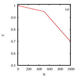
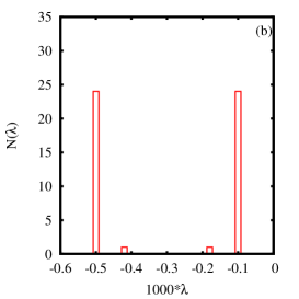
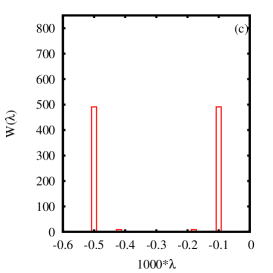
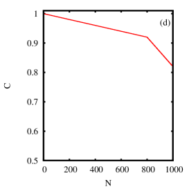
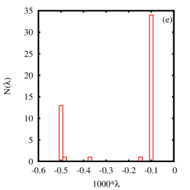
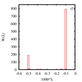
To demonstrate the difference in weights accounting take two–stage degradation data model from Ref. Bobyl et al. (2018b). Li–ion batteries capacity fade with each cycle, the degradation rate per cycle $dC/dN$ is the characteristics of interest. Consider $x=N$ and the measure $d\mu=dN$ (recent and old cycles are equally important), use $f(x)$ as battery degradation rate $f=dC/dN$. As in Ref. Bobyl et al. (2018b) consider $C(N)$ for 1000 cycles, the degradation rate for the first and second stages is $10^{-4}$ and $5\cdot 10^{-4}$ per cycle respectively. Two processes with first:second stages ratio as 500:500 ($f=-10^{-4}$ for $0\leq x\leq 500$ ; $f=-5\cdot 10^{-4}$ for $500\leq x\leq 1000$) and 800:200 ($f=-10^{-4}$ for $0\leq x\leq 800$ ; $f=-5\cdot 10^{-4}$ for $800\leq x\leq 1000$) are used as the model data, Fig. 1. In our previous worksBobyl et al. (2016, 2018b) we established, that the distribution of $\lambda^{[i]}$ from (8) is related to the distribution of $f$. In this paper this relation is found, the weights are (20) Lebesgue quadrature weights. Note, that for the data in Fig. 1, the peaks height for (c) and (f) correspond exactly to stage length, because of the measure chosen $d\mu=dN$.

A Lebesgue quadrature $(f^{[i]},w^{[i]})$ can be interpreted as $f(x)$ discrete distribution. The selection of value–nodes is optimal, such a quadrature performs optimal $n$–point discretization of $f(x)$. The approach is applicable to non–Gaussian distributions (e.g. with infinite standard deviation (but not with infinite mean), burst of many orders of magnitude, etc.). The situation is similar to the one in quantum mechanics: when a quantum Hamiltonian is known incorrectly and have some energy state, that is greatly different from the ground state, such a state does not change system behavior at all, because it has close to zero probability. The Lebesgue quadrature has similar ideology, it separates the state on: an observable value $f^{[i]}$ and the probability of it $w^{[i]}$. Similar path have been successfully tried earlier in our quantum–mechanics approach to machine learning of Ref. Malyshkin (2015c), where we separated system properties (described by the outcomes) and system testing conditions (described by the coverage).

Appendix A Density matrix, corresponding to a given polynomial

In Section II.2 the integral $\Braket{P(x)f(x)}$ with a polynomial $P(x)$ of a degree $2n-2$ or less is considered. The technique of Malyshkin and Bakhramov (2015) deals mostly with $\Braket{\psi^{2}(x)f(x)}=\Braket{\psi}{f}{\psi}$ type of integrals, and it is of practical value to be able to reduce a state described by an arbitrary polynomial:

$$P(x) =\sum_{k=0}^{2n-2}\gamma_{k}Q_{k}(x)$$ (30)

to the state described by the density matrix:

$$\rho(x,y) =\sum_{i=0}^{n-1}\lambda^{[i]}\psi^{[i]}(x)\psi^{[i]}(y)$$ (31)

$$P(x) =\rho(x,x)$$ (32)

such that $P(x)=\rho(x,x)$, and $\lambda^{[i]};\psi^{[i]}(x)$ are the eigenvalues and the eigenvectors of some operator $\|\rho\|$.

Theorem 3.

For a non–degenerated basis $Q_{k}(x)$ relatively the measure $d\mu$ such operator always exists and is generated by a measure with the moments $\Braket{Q_{k}(x)}_{P}$.

Proof.

To find a measure, such that $P(x)=\sum_{j,s,t,k=0}^{n-1}Q_{j}(x)\left[G^{-1}_{js}\Braket{Q_{s}Q_{t}}_{P}G^{-1}_{tk}\right]Q_{k}(x)$ (here $G^{-1}_{jk}$ is Gram matrix $G_{jk}=\Braket{Q_{j}Q_{k}}$ inverse) apply multiplication operator $c_{m}^{jk}$ from (29) to obtain:

$$\sum\limits_{m=0}^{2n-2}\gamma_{m}Q_{m}(x) =\sum\limits_{j,s,t,k=0}^{n-1}\,\sum\limits_{m=0}^{j+k}\,\sum\limits_{l=0}^{s+t}c_{m}^{jk}G^{-1}_{js}c_{l}^{st}G^{-1}_{tk}\Braket{Q_{l}}_{P}Q_{m}(x)$$ (33)

Comparing the coefficients by $Q_{m}(x)$ obtain a linear system of $2n-1$ dimension, from which the $\Braket{Q_{l}}_{P}$ ; $l=0\dots 2n-2$ moments can be found:

$$\sum\limits_{j,s,t,k=0}^{n-1}\,\sum\limits_{l=0}^{s+t}c_{m}^{jk}G^{-1}_{js}c_{l}^{st}G^{-1}_{tk}\Braket{Q_{l}}_{P} =\gamma_{m}$$ (34)

Then construct $\Braket{Q_{j}Q_{k}}_{P}$ Gram matrix of the measure corresponding to found moments $\Braket{Q_{l}}_{P}$, this gives the required $P(x)=\sum_{j,s,t,k=0}^{n-1}Q_{j}(x)G^{-1}_{js}\Braket{Q_{s}Q_{t}}_{P}G^{-1}_{tk}Q_{k}(x)$. To construct $\|\rho\|$ operator, eigenvalues/eigenvectors of which give (32): solve (8) generalized eigenvalue problem with the matrices $\Braket{Q_{j}Q_{k}}_{P}$ and $\Braket{Q_{j}Q_{k}}$ in (8) left– and right– hand side respectively, obtained eigenvalues/eigenvectors pairs give (32) expansion over the states of $\|\rho\|$ operator:

$$\sum\limits_{k=0}^{n-1}\Braket{Q_{j}Q_{k}}_{P}\alpha^{[i]}_{k} =\lambda^{[i]}\sum\limits_{k=0}^{n-1}\Braket{Q_{j}Q_{k}}\alpha^{[i]}_{k}$$ (35)

$$\rho(x,y) =\sum\limits_{i=0}^{n-1}\lambda^{[i]}\psi^{[i]}(x)\psi^{[i]}(y)=\sum\limits_{i=0}^{n-1}\Ket{\psi^{[i]}}\lambda^{[i]}\Bra{\psi^{[i]}}=\|\rho\|$$ (36)

$$P(x) =\rho(x,x)$$ (37)

∎

Remark.

The expansion of $P(x)=\sum_{j,s,t,k=0}^{n-1}Q_{j}(x)G^{-1}_{js}\Braket{Q_{s}Q_{t}}_{P}G^{-1}_{tk}Q_{k}(x)$ with the matrix $\Braket{Q_{j}Q_{k}}_{P}$ generated by a measure is unique, the measure moments are (34) linear system solution; without a requirement that the matrix to be generated by a measure, the solution is non–unique. Another non–uniqueness can arise from a degeneracy of $\Braket{Q_{j}Q_{k}}_{P}$ matrix, for example, take Christoffel function (14), $1/K(x)=P(x)=\sum_{j,k=0}^{n-1}Q_{j}(x)G^{-1}_{jk}Q_{k}(x)$: the solution (34) and the matrix $\Braket{Q_{j}Q_{k}}_{P}$ are unique, but the (32) expansion is non–unique due to (35) spectrum degeneracy (all the eigenvalues are equal to one), $1/K(x)=\sum_{i=0}^{n-1}\left[\phi^{[i]}(x)\right]^{2}$ for an arbitrary orthogonal basis $\Ket{\phi^{[i]}}$.

Note.

This prof is actually an algorithm to construct the density matrix $\|\rho\|$, producing a given polynomial $P(x)$. In provided implementation com/polytechnik/utils/BasisFunctionsMultipliable.java the method getMomentsOfMeasureProducingPolynomialInKK_MQQM(), for a given $P(x)$, solves the linear system (34) and obtains the moments $\Braket{Q_{m}}_{P}$. The method getDensityMatrixProducingGivenPolynomial() uses these moments to solve (35) and to obtain the $\|\rho\|$ from (36) as a Lebesgue quadrature, the spectrum of which corresponds to a given polynomial $P(x)$ (32).

From (32) it immediately follows that the sum of all $\|\rho\|$ eigenvectors is equal to $\Braket{P(x)}=\sum_{i=0}^{n-1}\lambda^{[i]}$, particularly for Christoffel function we have: $\Braket{1/K(x)}=\sum_{i=0}^{n-1}\lambda^{[i]}=n$, and in general case:

$$\Braket{f(x)P(x)} =\sum_{i=0}^{n-1}\lambda^{[i]}\Braket{\psi^{[i]}}{f}{\psi^{[i]}}$$ (38)

The (38) is a representation of $\Braket{f(x)P(x)}$ integral as a sum of $f$–moments over the states of the density matrix $\|\rho\|$ operator (35). This formula is a complementary one to (22), which is a representation of $\Braket{f(x)P(x)}$ integral as a sum of $P$–moments over the states of $\|f\|$ operator (8).

Finally, we want to emphasize, that used all of the above $\Braket{\psi}^{2}$ is a special case of a density matrix. Consider $\|\rho\|=\Ket{1}\Bra{1}$, then $\Braket{\psi}^{2}=\Braket{\psi}{\rho}{\psi}$, and for an operator $\|f\|$, $\Braket{f}=\mathrm{Spur}\,\|f|\rho\|$ Similarly, a spur with a density matrix $\|\rho\|$, e.g. corresponding to a polynomial $P(x)$, can be used instead of all averages:

$$\Braket{f} \to\mathrm{Spur}\,\|f|\rho\|$$ (39)

This way the approach we developed can be extended not only to polynomial by operator products study, but also to operator–by–operator products. Then, instead of $\mathrm{Spur}\,\|f|\rho\|$, which can be written either in (22) or in (38) representation, a general case of two operators $\mathrm{Spur}\,\|f|g\|$ can be considered. The first attempt to explore this direction is presented in Malyshkin (2018).

Appendix B On The Christoffel Function Spectrum

In the consideration above $f$ was a given function with finite moments $\Braket{Q_{j}}{f}{Q_{k}}$ in (2). It’s selection depends on the problem approached, for example we used $f=x$ to obtain Gaussian quadrature (11) and $f=dC/dN$ for Li–ion degradation rate study in Fig. 1. A question arise what the result we can expect if the Christoffel function (14) is used as $f(x)=K(x)=1\Big{/}\sum_{j,k=0}^{n-1}Q_{j}(x)G^{-1}_{jk}Q_{k}(x)$.

Theorem 4.

If $f(x)$ is equal to the Christoffel function $K(x)$ the eigenproblem

$$\sum\limits_{k=0}^{n-1}\Braket{Q_{j}}{K(x)}{Q_{k}}\alpha^{[i]}_{k} =\lambda^{[i]}_{K}\sum\limits_{k=0}^{n-1}\Braket{Q_{j}}{Q_{k}}\alpha^{[i]}_{k}$$ (40)

$$\psi^{[i]}_{K}(x) =\sum\limits_{k=0}^{n-1}\alpha^{[i]}_{k}Q_{k}(x)$$ (41)

has the sum of all eigenvalues $\lambda^{[i]}_{K}$ equals to the total measure:

$$\Braket{1} =\int d\mu=\sum_{i=0}^{n-1}\lambda^{[i]}_{K}$$ (42)

Proof.

For a given $n$ Christoffel function $K(x)$ vanishes at large $x$ with $1/x^{2n-2}$ asymptotic, the integrals (2) are finite and (40) has a solution with eigenvalues $\lambda^{[i]}_{K}$ (possibly degenerated) and eigenfunctions $\psi^{[i]}_{K}(x)$. The Christoffel function (14) can be expressed in any orthogonal basis, take $\phi^{[i]}(x)=\psi^{[i]}_{K}(x)$. From $\lambda^{[i]}_{K}=\Braket{\psi^{[i]}_{K}}{K(x)}{\psi^{[i]}_{K}}=\Braket{\left[\psi^{[i]}_{K}(x)\right]^{2}K(x)}$ and $K(x)=1\Big{/}\sum_{i=0}^{n-1}\left[\psi^{[i]}_{K}(x)\right]^{2}$ obtain $\Braket{1}=\sum_{i=0}^{n-1}\lambda^{[i]}_{K}$. ∎

The eigenfunctions (11) of a Gaussian quadrature correspond to $x$–localized states, they are $\|x\|$ operator eigenfunctions and the total weight is $\Braket{1}=\sum_{i=0}^{n-1}K(x^{[i]})$ with $w^{[i]}=K(x^{[i]})=\Braket{\psi^{[i]}}^{2}$; the $\psi^{[i]}(x)$ is (11) eigenproblem solution. The states $\psi^{[i]}_{K}(x)$ of (40) eigenproblem satisfy Theorem 4 and the Lebesgue quadrature weights sum (21): $\Braket{1}=\sum_{i=0}^{n-1}\Braket{\psi^{[i]}_{K}}{K(x)}{\psi^{[i]}_{K}}=\sum_{i=0}^{n-1}\Braket{\psi^{[i]}_{K}}^{2}$. However an eigenvalue $\lambda^{[i]}_{K}$ of (40) is not equal to the Lebesgue quadrature weight $\Braket{\psi^{[i]}_{K}(x)}^{2}$, see (46) below. A density matrix operator can be constructed from (40) eigenvalues and eigenfunctions:

$$\rho_{K}(x,y) =\sum\limits_{i=0}^{n-1}\lambda^{[i]}_{K}\psi^{[i]}_{K}(x)\psi^{[i]}_{K}(y)=\sum\limits_{i=0}^{n-1}\Ket{\psi^{[i]}_{K}}\lambda^{[i]}_{K}\Bra{\psi^{[i]}_{K}}=\|\rho_{K}\|$$ (43)

it is similar to ‘‘regular average’’ density matrix $\|\rho\|=\Ket{1}\Bra{1}$ considered in the Appendix A, e.g. both have the same Spur (equals to total measure). The (43) is the same as (36) but the eigenvalues/eigenfunctions are (40) instead of (35). The density matrix operator $\|\rho_{K}\|$ corresponds to the Christoffel function $K(x)$. The problem of averaging an operator $\|g\|$ with the Christoffel function used as a weight is a difficult problem Malyshkin (2015a). The (43) allows this problem to be approached directly: take the $\mathrm{Spur}\,\|g|\rho_{K}\|$. A question arise about $\|\rho_{K}\|\Leftrightarrow K(x)$ mapping: whether it is a one–to–one mapping or not? For $1/K(x)$, a polynomial of $2n-2$ degree, the mapping is (36). For $K(x)$ this requires a separate consideration. Anyway, built from the Christoffel function density matrix operator (43) allows us to consider an operator average with the Christoffel function in a regular ‘‘operatorish’’ way: by taking a Spur of operators product.

Recent progressMalyshkin (2019) in numerical computability of Radon–Nikodym derivative for multi–dimensional $\mathbf{x}$ allows us to demonstrate Theorem 4 numerically. Take a simple $d\mu=dx$ demonstration measure of the Appendix C of Malyshkin (2019):

$$d\mu =dx$$ (44)

$$x \in[-1:1]$$

The file dataexamples/runge_function.csv is bundled with provided software. It has 10001 rows (the measure support is split to 10000 intervals) and 9 columns. In the first seven columns there are the powers of $x$: $1,x,x^{2},x^{3},x^{4},x^{5},x^{6}$. Then, in the next two columns, follow: Runge function $1/(1+25x^{2})$ and the (44) weight. Run the program to obtain Christoffel function value for all observations in data file (column indexes are base 0):

java com/polytechnik/utils/RN --data_cols=9:0,6:1:8:1 \
      --data_file_to_build_model_from=dataexamples/runge_function.csv

Here as $f$ we use the $x$, the data is in the column with index $1$. The Lebesgue quadrature then produces the Gaussian quadrature for the measure (44):

$$x^{[0]} =-0.9491080257215085 w^{[0]} =0.1294848235792277 w_{K}^{[0]} =0.11746154871932572$$ (45)

$$x^{[1]} =-0.7415313130354606 w^{[1]} =0.279705429437816 w_{K}^{[1]} =0.2794795769155739$$

$$x^{[2]} =-0.40584522389537203 w^{[2]} =0.3818301175303132 w_{K}^{[2]} =0.38911964330481996$$

$$x^{[3]} =0 w^{[3]} =0.41795925890484187 w_{K}^{[3]} =0.42787846212051234$$

$$x^{[4]} =0.405845223895157 w^{[4]} =0.3818301175306451 w_{K}^{[4]} =0.38911964330486587$$

$$x^{[5]} =0.7415313130353846 w^{[5]} =0.2797054294378024 w_{K}^{[5]} =0.27947957691558917$$

$$x^{[6]} =0.9491080257213823 w^{[6]} =0.12948482357916594 w_{K}^{[6]} =0.11746154871930853$$

A small difference between (45) and exact values of 7-point Gaussian quadrature for the measure (44) is due to the fact that the moments calculation is not exact, they are calculated from 10001 discrete points in the file dataexamples/runge_function.csv. The Christoffel weights $w_{K}^{[i]}$ (48) are close to $w^{[i]}$ in case $f=x$. Created file runge_function.csv.RN.csv has 22 columns. First column is the label, next 7 columns are the powers of $x$ (copied from input), then $f=x$, weight, Radon–Nikodym derivative (26) of $fd\mu$ and $d\mu$ (here $f=x$), and the Christoffel function $K(x)$ (14) is in the column with index $12$; the other columns follow to total 22. Run the program again using the Christoffel function as $f$ (Christoffel function is in the column with index 12; an alternative is to use --flag_replace_f_by_christoffel_function=true):

java com/polytechnik/utils/RN --data_cols=22:1,7:12:9:0 \
      --data_file_to_build_model_from=runge_function.csv.RN.csv
or
java com/polytechnik/utils/RN --data_cols=9:0,6:1:8:1 \
      --flag_replace_f_by_christoffel_function=true \
      --data_file_to_build_model_from=dataexamples/runge_function.csv

The output file runge_function.csv.RN.csv.RN.csv now contains the eigenvalues $\lambda^{[i]}_{K}$ and the Lebesgue weights $w^{[i]}$ for eigenproblem (40) with the measure (44):

$$\lambda_{K}^{[0]} =0.10226835684407387 w^{[0]} =0.16153573777120298 w_{K}^{[0]} =0.10226835684403417$$ (46)

$$\lambda_{K}^{[1]} =0.12057295282629424 w^{[1]} =0 w_{K}^{[1]} =0.12057295282626747$$

$$\lambda_{K}^{[2]} =0.25910242661821975 w^{[2]} =0.4476418241676696 w_{K}^{[2]} =0.2591024266180915$$

$$\lambda_{K}^{[3]} =0.2924778951810179 w^{[3]} =0 w_{K}^{[3]} =0.2924778951809419$$

$$\lambda_{K}^{[4]} =0.37696956667653253 w^{[4]} =0.6388507741017023 w_{K}^{[4]} =0.37696956667633214$$

$$\lambda_{K}^{[5]} =0.4079988698735509 w^{[5]} =0 w_{K}^{[5]} =0.40799886987353334$$

$$\lambda_{K}^{[6]} =0.44060993198085746 w^{[6]} =0.751971663959237 w_{K}^{[6]} =0.44060993198079923$$

We see that for $f(x)=K(x)$ both: the eigenvalues sum and the Lebesgue quadrature weights sum are equal to total measure, it is $2$ for (44). Some of the Lebesgue quadrature weights are equal to $0$; for (44) measure Christoffel function is even, there are even and odd eigenfunctions, the average of odd eigenfunctions is zero. All Christoffel weights $w_{K}^{[i]}$ from (48) are non–zero and coincide with $\lambda_{K}^{[i]}$ because $f(x)=K(x)$, they will not coincide if optimal clustering to $D<n$ is performed with $\|\rho\|=\Ket{1}\Bra{1}$, see Appendix C below.

For a given $f(x)$ an eigenfunction $\psi^{[i]}(x)$ of eigenproblem (8) may possibly produce zero weight in the Lebesgue quadrature, this can be an inconvenient feature in a practical situation. The operator $\|\rho_{K}\|$ (43) allows us to introduce the ‘‘Christoffel weights’’ $w_{K}^{[i]}$, that are always positive. The operator $\|\rho_{K}\|$ Spur (42) is calculated in $\Ket{\psi^{[i]}_{K}}$ basis, it is equal to total measure $\Braket{1}$. The Spur is invariant with respect to basis transform, it will be the same when written in $\Ket{\psi^{[i]}}$ basis, (8) eigenvectors.

$$\Braket{1} =\sum_{i=0}^{n-1}\Braket{\psi^{[i]}_{K}}{\rho_{K}}{\psi^{[i]}_{K}}=\sum_{i=0}^{n-1}\Braket{\psi^{[i]}}{\rho_{K}}{\psi^{[i]}}$$ (47)

Define ‘‘Christoffel weights’’ $w_{K}^{[i]}$ as an alternative to the ‘‘Lebesgue weights’’ $w^{[i]}=\Braket{\psi^{[i]}}^{2}$ (20)

$$w_{K}^{[i]} =\Braket{\psi^{[i]}}{\rho_{K}}{\psi^{[i]}}=\Braket{\psi^{[i]}}{K(x)}{\psi^{[i]}}=\Braket{\frac{\left[\psi^{[i]}(x)\right]^{2}}{\sum_{j=0}^{n-1}\left[\psi^{[j]}(x)\right]^{2}}}$$ (48)

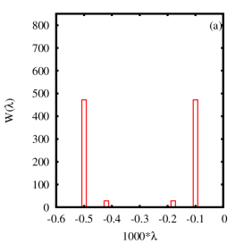
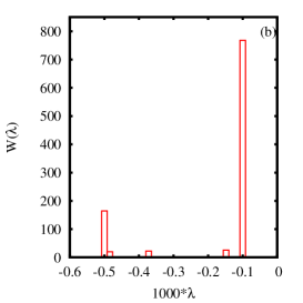
The weights $w_{K}^{[i]}$ satisfy the same normalizing condition (47) as the Lebesgue weights normalizing (21). In Fig. 2 the Christoffel weights are compared to (20) weights. One can see these weights are very close. However, the Christoffel weights $w_{K}^{[i]}$ have a property of being always positive and are related to Christoffel function operator $\|\rho_{K}\|$.

Figure 2: The same model as in Fig. 1, but with the Christoffel weights (48) instead of (20) weights; (a) corresponds to 1c and (b) corresponds to 1f. As in Fig. 1 the peak height corresponds exactly to the stage length because of chosen measure $d\mu=dN$. The calculations are performed for $n=50$ in polynomial basis.

The eigenvalues of (8) are the Lebesgue integral (15) value–nodes $f^{[i]}$, the weights are obtained from eigenfunction $\Ket{\psi^{[i]}}$ average. As we emphasized above in (39), any average corresponds to some density matrix. The $\|\rho\|=\Ket{1}\Bra{1}$ corresponds to a ‘‘regular’’ average, the Lebesgue weights then are: $w^{[i]}=\Braket{\psi^{[i]}}{\rho}{\psi^{[i]}}$. The $\|\rho_{K}\|$ corresponds to ‘‘Christoffel function average’’ with the weights (48).

The calculation of ‘‘Christoffel weights’’ requires one more matrix $\Braket{Q_{j}}{K(x)}{Q_{k}}$ to be calculated from the data sample. The cost to pay for the ‘‘Christoffel weights’’ is that the data sample now should be processed twice:

• Construct $\Braket{Q_{j}}{Q_{k}}$ and $\Braket{Q_{j}}{f}{Q_{k}}$.

• For every observation calculate Christoffel function $K(x)$ from the matrix $\Braket{Q_{j}}{Q_{k}}$. Build the matrix $\Braket{Q_{j}}{K(x)}{Q_{k}}$.

A second pass is required because Christoffel function matrix elements $\Braket{Q_{j}}{K(x)}{Q_{k}}$ go beyond basis function products and should be evaluated directly. In addition to the matrix of outcomes $\Braket{Q_{j}}{f}{Q_{k}}$ we now have a matrix of ‘‘coverage’’ $\Braket{Q_{j}}{K(x)}{Q_{k}}$ which is used to obtain operator $\|\rho_{K}\|$, corresponding to the Christoffel function $K(x)$. The Christoffel function can be considered as a ‘‘proxy’’ for coverageMalyshkin (2015a); Lasserre and Pauwels (2019); Beckermann et al. (2018): the number of observations that are ‘‘close enough’’ to a given $x$; but it can estimate only the coverage of a ‘‘localized’’ at $x$ state, not the coverage of a given state $\Ket{\psi}$. In contradistinction to the Christoffel function $K(x)$, the Christoffel function density matrix $\|\rho_{K}\|$ (43) can estimate the coverage of any given state $\Ket{\psi}$ as $\Braket{\psi}{\rho_{K}}{\psi}$; it is not limited to localized states as the Christoffel function $K(x)$ is.

A uniqueness of the Lebesgue quadrature makes it a very attractive tool for data analysis. When a data analysis problem defines some $f$, for example Li–ion degradation rate $f=dC/dN$ in Fig. 1, a class label in ML Malyshkin (2019), gray intensity in image reconstructionMalyshkin (2015d), etc. the solution $(\lambda^{[i]},\psi^{[i]})$ of (8) is unique and can be used as a basis for: PCA expansion (24), $f$ distribution estimation (20) or (48), optimal clustering of Appendix C, etc. There is a setup where a function $f$ either cannot be defined or is a multivalued function for which an eigenvalue problem cannot be formulated. However, we still want to obtain a unique basis that is constructed from the data sample, for example to avoid PCA dependence on attributes scale. In this case the most straightforward approach is to take the Christoffel function as $f(x)=K(x)$. This approach can be easily extended to a multi–dimensional $\mathbf{x}$, see Malyshkin (2019). An issue that often arise in case of a multi–dimensional $\mathbf{x}$ is a degeneracy of Gram matrix $G_{jk}=\Braket{Q_{j}Q_{k}}$. In the Appendix A of Malyshkin (2019) a regularization algorithm is presented, it needs to be applied to $\mathbf{x}$ to obtain a regularized basis $\mathbf{X}$. Then, in the regularized basis, the Christoffel function (14) can be calculated, the eigenproblem (40) solved, and a unique basis $\psi^{[i]}_{K}(x)$ obtained!

Appendix C On The Optimal Clustering Problem With A Density Matrix Average

The most noticeable result of our work Malyshkin (2019) is basis reduction algorithm, Section ‘‘Optimal Clustering’’. For $n$ input attributes (such as $Q_{k}(x)$ or multi–dimensional $\mathbf{x}$) construct $D\leq n$ linear combinations of them $\psi_{G}^{[m]}(x)$, $m=0\dots D-1$, that optimally separate $f$ in terms of $\Braket{f\psi^{2}}/\Braket{\psi^{2}}$. This solution is the key concept of our approach to data overfitting problem. A sketch of Malyshkin (2019) theory:

• Solve (8), obtain $n$ pairs $(f^{[i]}=\lambda^{[i]},\psi^{[i]})$. Introduce a measure $\Braket{\cdot}_{L}$

  $$\Braket{g(f)}_{L} =\sum_{i=0}^{n-1}g(f^{[i]})w^{[i]}$$ (49)

  $$w^{[i]} =\Braket{\psi^{[i]}}^{2}$$ (50)

• Construct a $D$–point Gaussian quadrature in $f$–space with the measure $\Braket{\cdot}_{L}$, obtain the functions $\psi_{G}^{[m]}(f)$ in $f$–space (Eq. (11) of dimension $D$ with $f$ used instead of $x$). The optimization problem in $f$–space is solved only once, all the solutions in $x$–space are obtained from the $\psi_{G}^{[m]}(f)$. This is different from Marx et al. (2019) where for every given $x$ a conditional minimization of the polynomial $1/K(\widetilde{x})$ is required: for a fixed $x$ in $\widetilde{x}=(x,f)$ find the $f$ providing the minimum.

• Convert the optimal clustering solution $\psi_{G}^{[m]}(f)$ from $f$–space to $x$–space, obtain $\psi_{G}^{[m]}(x)$. This conversion is possible only because the Lebesgue weights (50) are used in (49).

The Lebesgue weights $w^{[i]}=\Braket{\psi^{[i]}}^{2}$ correspond to a very specific form of the density matrix $\|\rho\|=\Ket{1}\Bra{1}$ (a ‘‘regular’’ average), this density matrix operator is a pure state. A question arise whether the optimal clustering success of Ref. Malyshkin (2019) can be repeated with a more general form of the density matrix, e.g. with the $\|\rho_{K}\|$ from (43)? Introduce a measure $\Braket{\cdot}_{L}$

$$\Braket{g(f)}_{L} =\sum_{i=0}^{n-1}g(f^{[i]})w^{[i]}$$ (51)

$$w^{[i]} =\Braket{\psi^{[i]}}{\rho}{\psi^{[i]}}$$ (52)

The weights (52) is the most general form of the Lebesgue weighs; (20) corresponds to $\|\rho\|=\Ket{1}\Bra{1}$.

As in Malyshkin (2019) a $D$–point Gaussian quadrature can be constructed from (51) measure, the eigenfunctions $\psi_{G}^{[m]}(f)$ are (11) eigenvectors with the replace: $n\rightarrow D$ and $x\rightarrow f$. They are orthogonal as

$$\delta_{ms} =\Braket{\psi_{G}^{[m]}(f)}{\psi_{G}^{[s]}(f)}_{L}$$ (53a)

$$\lambda_{G}^{[m]}\delta_{ms} =\Braket{\psi_{G}^{[m]}(f)}{f}{\psi_{G}^{[s]}(f)}_{L}$$ (53b)

$$w_{G}^{[m]} =\Braket{\psi_{G}^{[m]}}_{L}^{2}=\frac{1}{\left[\psi_{G}^{[m]}(\lambda_{G}^{[m]})\right]^{2}}$$ (53c)

The problem is to convert obtained optimal clustering solution $\psi_{G}^{[m]}(f)$ from $f$ to $x$ space; $D$ eigenvalues are denoted as $\lambda_{G}^{[m]}$ in order to not to mistake them with $n$ eigenvalues $f^{[i]}$ of (8). Introduce $D$ operators $\|\Psi_{G}^{[m]}\|$, ($m=0\dots D-1$; $i=0\dots n-1$):

$$\|\Psi_{G}^{[m]}\| =\sum\limits_{i=0}^{n-1}\Ket{\psi^{[i]}}\psi_{G}^{[m]}(f^{[i]})\Bra{\psi^{[i]}}$$ (54)

$$\Braket{A}_{\rho} =\mathrm{Spur}\,\|A|\rho\|$$ (55)

In the basis of (8) eigenproblem the operators $\|\Psi_{G}^{[m]}\|$ are diagonal. With (55) definition of average the orthogonality relation for $\|\Psi_{G}^{[m]}\|$ with respect to $\Braket{\cdot}_{\rho}$ is the same as (53) for $\psi_{G}^{[m]}(f)$ with respect to the measure $\Braket{\cdot}_{L}$:

$$\delta_{ms} =\Braket{\Psi_{G}^{[m]}}{\Psi_{G}^{[s]}}_{\rho}$$ (56a)

$$\lambda_{G}^{[m]}\delta_{ms} =\Braket{\Psi_{G}^{[m]}}{f}{\Psi_{G}^{[s]}}_{\rho}$$ (56b)

$$w_{G}^{[m]} =\Braket{\Psi_{G}^{[m]}}_{\rho}^{2}$$ (56c)

For $\|\rho\|=\Ket{1}\Bra{1}$ the $\psi_{G}^{[m]}(x)$ of Malyshkin (2019) can be expressed via the operators $\|\Psi^{[m]}_{G}\|$

$$\Ket{\psi_{G}^{[m]}} =\Ket{\Psi^{[m]}_{G}\Big{|}1}$$ (57)

$$p^{[m]}(x) =\left[\psi_{G}^{[m]}(x)\right]^{2}$$ (58)

$$f_{RN}(x) =\frac{\sum\limits_{m=0}^{D-1}\lambda_{G}^{[m]}p^{[m]}(x)}{\sum\limits_{m=0}^{D-1}p^{[m]}(x)}$$ (59)

$$f_{RNW}(x) =\frac{\sum\limits_{m=0}^{D-1}\lambda_{G}^{[m]}p^{[m]}(x)w_{G}^{[m]}}{\sum\limits_{m=0}^{D-1}p^{[m]}(x)w_{G}^{[m]}}$$ (60)

The optimal clustering states $\psi_{G}^{[m]}(f)$ can only be converted to pure states in $x$–space $\psi_{G}^{[m]}(x)$ when the density matrix $\|\rho\|$ is of a pure state form $\Ket{\varphi}\Bra{\varphi}$, otherwise the conversion to $x$–space produces mixed states described by the operators $\|\Psi_{G}^{[m]}\|$. While the $\psi_{G}^{[m]}(x)$ does not exist for a general $\|\rho\|$, the $p^{[m]}(x)$ weight, required to obtain Radon–Nikodym interpolation (59) and classification (60) solutions, can always be obtained. From (54) it follows that

$$p^{[m]}(x) =\Braket{\psi_{x}\Big{missing}}{\Psi_{G}^{[m]}}{\rho|\Psi_{G}^{[m]}|\psi_{x}}=\sum\limits_{i,j=0}^{n}\psi^{[i]}(x)\psi^{[j]}(x)\psi_{G}^{[m]}(f^{[i]})\psi_{G}^{[m]}(f^{[j]})\Braket{\psi^{[i]}}{\rho}{\psi^{[j]}}$$ (61)

For $\|\rho\|=\Ket{1}\Bra{1}$ (61) becomes (58). A very important feature of the Radon–Nikodym approach (59) is that it can be generalized to the density matrix states. The $\left[\psi_{G}^{[m]}(x)\right]^{2}$ used as an eigenvalue weight needs to be replaced by a more general form (61). Thus all the optimal clustering results of Ref. Malyshkin (2019) are now generalized from the weights (20) to the weights $\Braket{\psi^{[i]}}{\rho}{\psi^{[i]}}$, described by a density matrix $\|\rho\|$ of the most general form, e.g. by the Christoffel function density matrix (43).

Appendix D Usage Example of com/polytechnik/algorithms/ExampleRadonNikodym_F_and_DF.java

The com/polytechnik/algorithms/ExampleRadonNikodym_F_and_DF.java is a program processing 1D data. It was used in Bobyl et al. (2016) to obtain relaxation rate distribution. In contrast with advanced multi–dimensional approach of Malyshkin (2019), this program has a rigid interface and limited functionality. It is bundled with provided software. Usage example to reproduce Fig. 1 data: Create a two–stage linear model of Fig. 1d with 800:200 lengths, save the model to slope_800_200.csv.

java com/polytechnik/algorithms/PrintFunTwoLinearStages \
     slope_800_200.csv 10000 1000 800 1e-4 5e-4 0

Solve (8) for $f=dC/dN$ ($f=C$ is also calculated). Use $n=50$ and the data from slope_800_200.csv.

java com/polytechnik/algorithms/ExampleRadonNikodym_F_and_DF \
     slope_800_200.csv 50 sampleDX

The files slope_800_200.csv.QQdf_QQ_spectrum.dat and slope_800_200.csv.QQdf_QQ_spectrum.dat are generated. They correspond to $f=dC/dN$ and to $f=C$ respectively. The files contain 5 columns: eigenvalue index, eigenvalue $\lambda^{[i]}$, $x_{\psi^{[i]}}=\Braket{\psi^{[i]}}{x}{\psi^{[i]}}/\Braket{\psi^{[i]}}{\psi^{[i]}}$, $w^{[i]}$ weight (20), and $w_{K}^{[i]}$ weight (48). The data can be grouped to 25 bins of $\lambda^{[i]}$ (the column with index 1) to produce Fig. 1f (the weight is in the column with index 3) and Fig. 2b (the weight is in the column with index 4).

java com/polytechnik/algorithms/HistogramDistribution \
     slope_800_200.csv.QQdf_QQ_spectrum.dat 5:1:3 25 >W_800_200.csv
java com/polytechnik/algorithms/HistogramDistribution \
     slope_800_200.csv.QQdf_QQ_spectrum.dat 5:1:4 25 >WK_800_200.csv

References

- Totik (11 Nov. 2005) Vilmos Totik, ‘‘Orthogonal polynomials,’’ Surveys in Approximation Theory 1, 70–125 (11 Nov. 2005).
- Beckermann (1996) Bernhard Beckermann, On the numerical condition of polynomial bases: estimates for the condition number of Vandermonde, Krylov and Hankel matrices, Ph.D. thesis, Habilitationsschrift, Universität Hannover (1996).
- Malyshkin and Bakhramov (2015) Vladislav Gennadievich Malyshkin and Ray Bakhramov, ‘‘Mathematical Foundations of Realtime Equity Trading. Liquidity Deficit and Market Dynamics. Automated Trading Machines.’’ ArXiv e-prints (2015), http://arxiv.org/abs/1510.05510, arXiv:1510.05510 [q-fin.CP] .
- Wikipedia (2016) Wikipedia, ‘‘Bra–ket notation,’’ (2016).
- Kolmogorov and Fomin (8 May 2012) A. N. Kolmogorov and S. V. Fomin, Elements of the Theory of Functions and Functional Analysis (Martino Fine Books (May 8, 2012), 8 May 2012).
- Bobyl et al. (2016) Aleksandr Vasilievich Bobyl, Andrei Georgievich Zabrodskii, Mikhail Evgenievich Kompan, Vladislav Gennadievich Malyshkin, Olga Valentinovna Novikova, Ekaterina Evgenievna Terukova, and Dmitry Valentinovich Agafonov, ‘‘Generalized Radon–Nikodym Spectral Approach. Application to Relaxation Dynamics Study.’’ ArXiv e-prints (2016), https://arxiv.org/abs/1611.07386, arXiv:1611.07386 [math.NA] .
- Malyshkin (2017) Vladislav Gennadievich Malyshkin, ‘‘Market Dynamics. On A Muse Of Cash Flow And Liquidity Deficit,’’ ArXiv e-prints (2017), arXiv:1709.06759 [q-fin.TR] .
- Gautschi (2004) Walter Gautschi, Orthogonal polynomials: computation and approximation (Oxford University Press on Demand, 2004).
- Killip and Simon (2003) Rowan Killip and Barry Simon, ‘‘Sum rules for jacobi matrices and their applications to spectral theory,’’ Annals of mathematics , 253–321 (2003).
- Malyshkin (2019) Vladislav Gennadievich Malyshkin, ‘‘On The Radon–Nikodym Spectral Approach With Optimal Clustering,’’ arXiv preprint arXiv:1906.00460 (2019), arXiv:1906.00460 [cs.LG] .
- Nevai (1986) Paul G Nevai, ‘‘Géza Freud, Orthogonal Polynomials. Christoffel Functions. A Case Study,’’ Journal Of Approximation Theory 48, 3–167 (1986).
- Simon (2011) Barry Simon, Szegő’s Theorem and Its Descendants (Princeton University Press, 2011).
- Bernard (2009) Lasserre Jean Bernard, Moments, positive polynomials and their applications, Vol. 1 (World Scientific, 2009).
- Malyshkin (2015a) Vladislav Gennadievich Malyshkin, ‘‘Multiple–Instance Learning: Christoffel Function Approach to Distribution Regression Problem,’’ ArXiv e-prints (2015a), arXiv:1511.07085 [cs.LG] .
- Malyshkin (2015b) Vladislav Gennadievich Malyshkin, ‘‘Multiple-Instance Learning: Radon-Nikodym Approach to Distribution Regression Problem,’’ ArXiv e-prints (2015b), arXiv:1511.09058 [cs.LG] .
- Malyshkin (2015c) Vladislav Gennadievich Malyshkin, ‘‘Norm-Free Radon-Nikodym Approach to Machine Learning,’’ ArXiv e-prints (2015c), http://arxiv.org/abs/1512.03219, arXiv:1512.03219 [cs.LG] .
- Malyshkin (2018) Vladislav Gennadievich Malyshkin, ‘‘On Numerical Estimation of Joint Probability Distribution from Lebesgue Integral Quadratures,’’ ArXiv e-prints (2018), arXiv:1807.08197 [math.NA] .
- Lapack (2013) Lapack, ‘‘Lapack version 3.5.0,’’ (2013).
- Malyshkin (2015d) Vladislav Gennadievich Malyshkin, ‘‘Radon–Nikodym approximation in application to image reconstruction.’’ ArXiv e-prints (2015d), http://arxiv.org/abs/1511.01887, arXiv:1511.01887 [cs.CV] .
- Malyshkin (2014) Vladislav Gennadievich Malyshkin, (2014), the code for polynomials calculation, http://www.ioffe.ru/LNEPS/malyshkin/code.html.
- Bobyl et al. (2018a) A.V. Bobyl, V.V. Davydov, A.G. Zabrodskii, N.R. Kostik, V.G. Malyshkin, O.V. Novikova, D.M. Urishov, and E.A. Yusupova, ‘‘The Spectral approach to timeserie bursts analysis (Спектральный подход к анализу всплесков временной последовательности),’’ ISSN 0131-5226.Теоретический и научно-практический журнал. ИАЭП. , 77–85 (2018a), doi:10.24411/0131-5226-2018-10010.
- Bobyl et al. (2018b) Aleksandr Vasilievich Bobyl, Andrei Georgievich Zabrodskii, Vladislav Gennadievich Malyshkin, Olga Valentinovna Novikova, Evgeny Ivanovich Terukov, and Dmitry Valentinovich Agafonov, ‘‘Generalized Radon–Nikodym Approach to Direct Estimation of Degradation Rate Distribution. (Деградация Li-ion накопителей энергии. Применение обобщенного подхода Радона–Никодима к оценке распределения скоростей деградации.),’’ Izversiya RAN. Energetika. (Известия РАН. Энергетика) , 46–58 (2018b).
- Guhr et al. (1998) Thomas Guhr, Axel Müller-Groeling, and Hans A Weidenmüller, ‘‘Random-matrix theories in quantum physics: common concepts,’’ Physics Reports 299, 189–425 (1998).
- Lasserre and Pauwels (2019) Jean B Lasserre and Edouard Pauwels, ‘‘The empirical christoffel function with applications in data analysis,’’ Advances in Computational Mathematics , 1–30 (2019).
- Beckermann et al. (2018) Bernhard Beckermann, Mihai Putinar, Edward B Saff, and Nikos Stylianopoulos, ‘‘Perturbations of Christoffel-Darboux kernels. I: detection of outliers,’’ arXiv preprint arXiv:1812.06560 (2018).
- Marx et al. (2019) Swann Marx, Edouard Pauwels, Tillmann Weisser, Didier Henrion, and Jean Lasserre, ‘‘Tractable semi-algebraic approximation using Christoffel-Darboux kernel,’’ arXiv preprint arXiv:1904.01833 (2019).