XMMPZCAT: A catalogue of photometric redshifts for X-ray sources

Abstract

Aims. The third version of the XMM-Newton serendipitous catalogue (3XMM), containing almost half million sources, is now the largest X-ray catalogue. However, its full scientific potential remains untapped due to the lack of distance information (i.e. redshifts) for the majority of its sources. Here we present XMMPZCAT, a catalogue of photometric redshifts (photo-z) for 3XMM sources.

Methods. We searched for optical counterparts of 3XMM-DR6 sources outside the Galactic plane in the SDSS and Pan-STARRS surveys, with the addition of near- (NIR) and mid-infrared (MIR) data whenever possible (2MASS, UKIDSS, VISTA-VHS, and AllWISE). We used this photometry data set in combination with a training sample of 5157 X-ray selected sources and the MLZ-TPZ package, a supervised machine learning algorithm based on decision trees and random forests for the calculation of photo-z.

Results. We have estimated photo-z for 100 178 X-ray sources, about 50% of the total number of 3XMM sources (205 380) in the XMM-Newton fields selected to build this catalogue (4208 out of 9159). The accuracy of our results highly depends on the available photometric data, with a rate of outliers ranging from 4% for sources with data in the optical+NIR+MIR, up to $\sim 40\%$ for sources with only optical data. We also addressed the reliability level of our results by studying the shape of the photo-z probability density distributions.

1 Introduction

The third version of the XMM-Newton serendipitous catalogue, data release six, (3XMM-DR6) contains about 500 000 unique sources covering a total area of 1000 deg² on the sky. Two thirds of these are located at high Galactic latitude, —b—¿20 deg. Recently, the catalogue has been enriched with added-value products thanks to the XMMFITCAT (Corral et al., 2015), ARCHES (Motch et al., 2016) and EXTraS (e.g. Pizzocaro et al., 2016) projects. The first provides the spectral fit inventory of 157 000 sources with the highest photon statistics while the second is providing multi-wavelength positional cross-matches using Bayesian statistics. The third project will provide the characterisation of X-ray variable sources.

Although the vast majority of these nearly 500 000 sources are expected to be active galactic nuclei (AGN), the huge potential of the 3XMM catalogue remains practically untapped because most of the sources lack redshift information. Spectroscopy is expensive and challenging for such a large sample. Therefore, photometric redshifts (photo-z) is the only feasible way to estimate distances for half a million sources. However, photo-z are subject to systematics and higher uncertainties compared to spectroscopic redshifts (spec-z).

Many photo-z estimation methods have been developed in pursuit of deriving the most accurate photo-z. These methods can be divided into two main categories: template-fitting (e.g. Bolzonella et al., 2000) and machine-learning (e.g. D’Isanto & Polsterer, 2018) techniques.

Among the variety of methods developed using template-fitting techniques we can mention for instance Bayesian photometric redshifts (BPZ; Benítez, 2000) or Easy and Accurate photo-Z from Yale (EAZY; Brammer et al., 2008). In the case of machine learning techniques, a growing number of methods have been published in recent years, using different machine learning algorithms, from neural networks, for example artificial neural network (ANNz; Collister & Lahav, 2004; Lahav & Collister, 2012), to random forest techniques, for example, Trees for Photo-Z (TPZ; Carrasco Kind & Brunner, 2013). Each of these methods has its own advantages and disadvantages (see Abdalla et al. 2011; Beck et al. 2017 for detailed comparisons among the various photo-z estimation methods). Mixed techniques are also used, where spectral energy distribution (SED) fitting methods rely on a previous machine-learning classification to select the most adequate set of templates (e.g. Fotopoulou et al., 2016).

Supervised machine-learning techniques, also known as empirical methods, require a spectroscopic sample to train an algorithm. Then the algorithm is applied to a dataset with available photometry to estimate photometric redshifts. These methods have been extensively applied on galaxy samples (e.g. SDSS, Beck et al., 2016) and optical QSOs (e.g. Ball et al., 2007, 2008; D’Isanto & Polsterer, 2018). For X-ray AGN, though, only SED fitting techniques had been used (Salvato et al., 2009; Hsu et al., 2014), up until recently. This was due to lack of large enough X-ray spectroscopic training sets. Mountrichas et al. (2017) presented a catalogue with $\sim 1000$ X-ray sources in the X-ATLAS field using, for the first time, a machine learning technique (TPZ; Carrasco Kind & Brunner, 2013). Their training, spectroscopic sample consists of 5157 sources primarily in the XMM-XXL field (Liu et al., 2016; Menzel et al., 2016).

Here we present the XMM-Newton Photo-Z CATalogue (XMMPZCAT). Using the training set presented in Mountrichas et al. (2017), we estimate photometric redshifts for $\sim 100\,000$ 3XMM sources with at least optical photometry available (SDSS or Pan-STARRS). We provide estimations of the accuracy of our photo-z estimations as well as the percentage of outliers.

The structure of the paper is as follows: in Sect. 2 we describe the 3XMM sample as well as the catalogues used to obtain photometric information for our X-ray sources. In Sect. 3 we present the methods used for the cross-match among the various datasets and in Sect. 4 we briefly describe the TPZ algorithm and the training sample. The results are presented in Sect. 5, while we summarise the main conclusions of our analysis in Sect. 6.

2 Data

Optical photometry is needed to derive photometric redshifts, so we explored several wide-angle surveys to maximise the number of counterparts of our X-ray sources. We also complemented these data with photometry in the near- and mid-infrared to increase the accuracy of the photometric redshifts. A brief description of all catalogues we used is presented below.

2.1 3XMM

3XMM-DR6 catalogue (Rosen et al., 2016) was released in July 2016. It contains 9160 observations, covering an energy interval from 0.2 keV to 12 keV. The net sky area observed is $\sim$ 1032 deg². 468 440 unique X-ray sources are included in the catalogue with a median flux in the total energy band of $\sim 2.4\times 10^{-14}\leavevmode\nobreak\ \mathrm{erg\,cm^{-2}\,s^{-1}}$.

2.2 SDSS

Data release 13 of the Sloan digital sky survey (SDSS-DR13; Albareti et al., 2017) is the first data release of the fourth phase of the SDSS and covers 14 555 deg², more than one-third of the entire celestial sphere. This release does not include new or updated photometric information beyond that already included in the SDSS-DR9 (Ahn et al., 2012), but the imaging data have been photometrically re-resolved and recalibrated. The catalogue contains about 500 million unique, primary sources providing optical photometry for about 95% of the point sources in five bands: u, g, r, i, z. The magnitude limit is $r_{AB}=22.2$ mag. Among the various measures of magnitude that offers the SDSS, we used the composite model magnitudes (cModelMag). These magnitudes are suitable for both extended and point-like sources.

2.3 Pan-STARRS

Pan-STARRS1 (PS1; Flewelling et al., 2016) is the first data release from the panoramic survey telescope and rapid response system (Pan-STARRS; Chambers et al., 2016). Pan-STARRS uses a 1.8 metre telescope to image the sky. It exploits the combination of relatively small mirrors with very large digital cameras to observe the entire available sky several times each month. 3$\pi$ of the sky are covered north of declination -30 deg, in five broad-band filters: g, r, i, z, y. The magnitude limits reach g=23.3, r=23.2, i=23.1, z=22.3, and y=21.3.

Whenever available, we used the stack photometry (i.e. the magnitudes estimated using the stacking of all available PS1 observations of the source), otherwise we used the mean photometry. For objects classified as point-like by the PS1 pipeline, we used the corresponding PSF magnitudes. For extended objects, we used the Kron magnitudes.

2.4 AllWISE

NASA’s wide-field infrared survey explorer (WISE; Wright et al., 2010) mapped the sky in the mid-infrared (MIR) at 3.4, 4.6, 12, and 22 $\mu$m (W1, W2, W3, W4). WISE achieved 5$\sigma$ point source sensitivities better than 0.08, 0.11, 1 and 6 mJy in unconfused regions on the ecliptic in the four bands. Sensitivity improves towards the ecliptic poles due to denser coverage and lower zodiacal background. The AllWISE source catalogue (Cutri et al., 2013) contains the attributes for over 747 million objects detected at SNR¿5 in at least one band in the combined exposures of the atlas intensity images.

2.5 2MASS

The 2 micron all sky survey (2MASS; Skrutskie et al., 2006) uniformly scanned the entire sky in three near-infrared (NIR) bands, J, H, K_S. The magnitude limits are J=15.8/15.0, H=15.1/14.3 and K${}_{S}=14.3/13.5$ for point-like or extended sources, correspondingly. We used the 2MASS point-source catalogue (Cutri et al., 2003), which includes over 300 million objects.

2.6 UKIDSS

The UKIRT (Casali et al., 2007) infrared deep sky survey (UKIDSS; Lawrence et al., 2007), successor to 2MASS, started in 2005 and has surveyed 7500 deg² on the Northern sky in YJHK down to a magnitude limit of K=18.4 (Vega) in its shallowest parts (UKIDSS-LAS, 4000 deg²). This depth is three magnitudes deeper than 2MASS. We have used the data release ten of UKIDSS-LAS, the most recent release (November 2014) publicly available. Only J, H and K magnitudes were used in our cross-match.

2.7 VISTA-VHS

The visible and infrared survey telescope for astronomy (VISTA; Lawrence et al., 2007) is an ESO’s 4 metre class wide field survey telescope for the southern hemisphere, equipped with a near infrared camera. The VISTA-VHS (VISTA hemisphere survey; McMahon et al., 2013) is one of the six large public surveys conducted by VISTA to image the entire southern hemisphere of the sky ($\sim 20\,000\leavevmode\nobreak\ \mathrm{deg}^{2}$), with the exception of the areas already covered by other vista surveys surveys, in J and K_S bands, plus Y and H bands for the high Galactic latitude ($|b|>30$ deg) sky. VISTA-VHS has a depth advantage of over four magnitudes relative to previous NIR surveys like 2MASS or DENIS (Epchtein et al., 1994), and $\sim 1.3$ magnitudes relative to the UKIDSS-LAS. The magnitude limits are J=20.2, H=19.4 and K${}_{S}=18.1$. We used data from VHS-DR4, the last data release publicly available (March 2017).

3 Identification of counterparts

Our first step in building XMMPZCAT was the identification of optical counterparts for the X-ray sources in the 3XMM and, whenever possible, counterparts in the NIR and/or MIR bands. We looked for optical counterparts using two large area surveys: SDSS and PS1. For the SDSS, we used the multi-wavelength catalogues from the ARCHES project (see Sect.3.1 below). For PS1, we did our own cross-matching of 3XMM and PS1 (see Sect.3.2), plus the NIR and MIR catalogues described above, using the cross-matching tool and techniques developed by ARCHES.

There are other tools that offer basic cross-matching algorithms (e.g. TOPCAT; Taylor, 2005), or even more advanced techniques using ‘Bayes’ factors’ (Budavári & Szalay, 2008) that combine astrometric and photometric information (Georgakakis & Nandra, 2011), but none of these handle the statistics inherent to the crossmatching process in a fully coherent manner, particularly when combining the information from more than two catalogues. A proper statistical treatment is of great importance when dealing with catalogues where the positional uncertainties are significantly different, which is usually the case if X-ray catalogues are included. For example, the average error in the 3XMM is $\sim 2$ arcsec, while in optical catalogues like SDSS or Pan-STARRS is one or even two orders of magnitude lower.

The design of a crossmatching tool with such capabilities was one of the major goals of ARCHES. Recently, an alternative tool with similar capabilities has been developed (NWAY; Salvato et al., 2018).

3.1 3XMMe-SDSS (ARCHES)

The astronomical resource cross-matching for high energy studies (ARCHES) project is an European consortium created with the objective of building scientifically-validated spectral energy distributions for the many X-ray sources detected by the XMM-Newton observatory. To this end, ARCHES developed the enhanced 3XMM catalogue data (3XMMe) and new tools for the cross-correlation of extensive astronomical catalogues. See Motch et al. (2016) for further details.

Among the main deliverables of the ARCHES project, two multi-wavelength cross-matched catalogues were released. The base X-ray catalogue used in the cross-matching was 3XMMe. This catalogue is based on the 3XMM-DR5 catalogue and it was built by carefully removing detections that are considered to be of lower scientific reliability or quality, as well as fields that have been the subject of dedicated studies and/or overlap with large, well known objects. As a result, 3XMMe is smaller than 3XMM-DR5, but composed of X-ray sources from XMM-Newton observations with the highest quality.

The first of the multi-wavelength cross-matched catalogues is the result of the cross-correlation of 3XMMe with GALEX-DR5 (Bianchi et al., 2014), UCAC4 (Zacharias & Gaume, 2011), SDSS, 2MASS, AllWISE, the merge of SUMSS and NVSS (Mingo et al., 2016), and the AKARI-FIS (Doi et al., 2015) catalogues. The second one is similar, although smaller, since 2MASS is replaced by UKIDSS-LAS, which is not an all-sky survey. Probabilities of associations were computed, by using the xmatch tool (see Sect. 3.2), for all possible sets of candidates in the first five catalogues, whereas candidates from SUMSS, NVSS and AKARI-FIS were selected based on a $\chi^{2}$ criteria.

We were interested in finding counterparts in the optical (SDSS), NIR (2MASS or UKIDSS), and MIR (WISE). Therefore, we rejected all sources with no counterparts in at least one of these catalogues. Moreover, we only kept counterparts with photometry in all the corresponding filters of each catalogue. For example, if an X-ray source has counterparts in the NIR and the optical, but the NIR source has no photometry in the J filter, we rejected the NIR counterpart and considered that the X-ray source has only an optical counterpart. If the optical source has no photometry in one or more SDSS filters, the X-ray source is not included in our selection.

We did a second filtering based on the probabilities of association given in the ARCHES catalogue. However, since these probabilities take into account all the catalogues where the counterparts were found, we had to derive the probabilities of associations for the cases we were interested in, as a function of the ones provided in the ARCHES catalogues, that is, we estimated the marginal probabilities for the optical, optical+NIR, optical+MIR, and optical+NIR+MIR according to each case.

We then selected sources with probabilities of association larger than 68%. The same X-ray source can appear multiple times in the ARCHES catalogue, associated with a different set of optical, NIR, and/or MIR counterparts. In those cases we kept the association with the largest number of counterparts. If the number of counterparts was the same, we preferred the association having MIR data. If both associations (or none) had MIR data, we just kept the one with the highest probability.

Applying this method, we finally obtained a multi-wavelength catalogue composed of 42 705 X-ray sources with SDSS counterparts (u, g, r, i, and z magnitudes), 14 805 of them with near-infrared counterparts (UKIDSS or 2MASS; J, H, and K/K_S magnitudes), and 26 926 of them with WISE counterparts (W1 and W2 magnitudes). According to the distribution of association probabilities obtained in the ARCHES catalogue, we expect about 3660 miss-matches ($\sim 9\%$) in this catalogue.

3.2 3XMM-Pan-STARRS (XPS)

Using data from PS1 we can increase the size of our final catalogue of photometric redshift, since it covers a larger sky area than the SDSS. Moreover, we can also include a significant fraction of the 3XMM sources not included in the ARCHES catalogue, either because they were rejected from the 3XMMe, or were new sources added in the 3XMM-DR6

We did our own cross-matching of PS1 and 3XMM-DR6 catalogues. Since we are interested in obtaining photometry in the NIR and MIR bands, we also included AllWISE, 2MASS, UKIDSS and VISTA-VHS surveys in the cross-match. We used the xmatch tool for this multi-catalogue cross-matching. This tool estimates the probability that a tuple of sources from different catalogues corresponds to the same real source (see Pineau et al. 2017 for a complete description of the algorithm).

xmatch uses a Bayesian approach to estimate this probability, taking into account the likelihoods and priors of all possible hypotheses (e.g. all sources in the tuple are associated with different real sources, two sources in the tuple are associated with one real source and the rest to other source, etcetera). Likelihoods depend on the corresponding hypothesis, the number of cross-matched catalogues, and the Mahalanobis distance (Mahalanobis, 1936; De Maesschalck et al., 2000) between sources in the tuple, essentially an error weighted average of the positional distance. Priors, an estimation of the probability that a particular hypothesis is obtained by chance, critically depend on the density of sources for each catalogue in the cross-matched area. Hence, to obtain meaningful probabilities the software has to be able to correctly estimate these densities.

xmatch cross-matches the catalogues using defined fields of common areas in all catalogues. These fields should be large enough to obtain an estimation of the source densities free of large statistical variance. In our case, the most straightforward way of defining the fields is through the XMM-Newton observations included in the 3XMM. The XMM-Newton field of view can be approximated by a circle of 15 arcmin radius. We selected all 3XMM observations included in the PS1 footprint (declination greater than -30 deg), except those flagged as OBS_CLASS$>3$ (more than 10% of the area of the observed field is identified as bad), or otherwise the compared areas between the 3XMM and the remaining catalogues would be significantly different. Since some of these observed fields have common areas, we grouped those overlapping fields in a single field. We end up with 2623 non-overlapping fields, covering a total of $\sim 630\;\mathrm{deg^{2}}$ ($\sim 466\;\mathrm{deg^{2}}$ outside the Galactic plane). All PS1, 2MASS and AllWISE sources within these fields were considered potential counterparts by xmatch, in addition to the corresponding UKIDSS-LAS and VISTA-VHS sources, if the field was included in those surveys.

However, the areas of most of these fields are not large enough to obtain a good estimation of the density of X-ray sources. This density depends mostly on the exposure time of the corresponding XMM-Newton observation (see Fig. 1, bottom).. By grouping fields of similar exposure time we can reduce the statistical variance and get a better estimation of the density of the X-ray sources. We must also take into account that the density of PS1 sources depends on the Galactic latitude (Fig. 1, top). Based on these two parameters, we grouped the 2623 fields in bins with roughly constant densities of X-ray and optical sources. Using this method, we defined 70 different bins, with sky areas ranging between $\sim 4-20\;\mathrm{deg^{2}}$, and we run xmatch for each one.

Figure 1: Sky density of sources for the 2623 non-overlapping fields we defined in the 3XMM/PS1 cross-match. Blue circles show the density of optical sources, green triangles the density of X-ray sources (darker shades show a higher density of data points). Top: Sky density versus the absolute value of the Galactic latitude. Bottom: Sky density versus exposure time of the XMM-Newton observation.

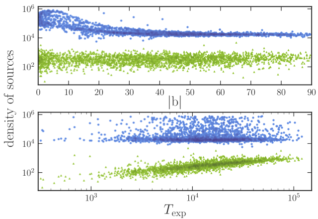
Given the high density of optical sources in the Galactic plane, the association probabilities calculated by xmatch in this area are extremely low. A large difference in the density of sources of two catalogues implies that the probability of association by chance is very high. In the Galactic plane the difference between the density of optical and X-ray sources can reach up to four orders of magnitude (see Fig. 1). We therefore decided to reject those sources from our catalogue and to keep only objects outside the Galactic plane (i.e. $|b|>20$ deg).

For consistency with the ARCHES data set, for building our final catalogue we followed the same photometry- and probability-based selection criteria we explained in Sect. 3.1 above. The only difference is that we did not marginalise the probabilities of association, because our cross-match did not contain catalogues we were not interested in. Therefore, the xmatch output directly gave us the proper probabilities.

Our final 3XMM/Pan-STARRS catalogue (XPS) is composed of 88 088 X-ray sources with PS1 counterparts (g, r, i, z, and y magnitudes), 21 174 of them with NIR counterparts (2MASS, UKIDSS or VISTA-VHS, J, H, and K or K_S magnitudes), and 54 947 of them with MIR (All-WISE, W1 and W2 magnitudes) counterparts. According to the distribution of association probabilities given by xmatch, we expect about 8100 miss-matches ($\sim 9\%$) in this catalogue.

4 Photometric redshifts

We used a supervised machine-learning technique to estimate photometric redshifts for XMMPZCAT. These techniques require a spectroscopic sample to train an algorithm (Sect. 4.1). Then the algorithm is applied to a dataset with available photometry to estimate photometric redshifts.

Our photo-z determination is primary based on the five optical bands available in SDSS and PS1: g, r, i, z, plus u or y respectively, depending on the optical catalogue we are using. We tested that including photometric points beyond the optical range significantly improves the accuracy of photo-z (see also e.g. Ball et al., 2007; Rowan-Robinson et al., 2008; Yang et al., 2017), and decrease the number of outliers. Hence, whenever available we have also used NIR and/or MIR photometry to derive the photometric redshifts.

Photometric redshifts were estimated using MLZ-TPZ (Carrasco Kind & Brunner, 2013), a machine-learning algorithm based on a supervised technique with prediction trees and random forest. It is a parallelizable python package that calculates fast and robust photometric redshifts and their corresponding probability density functions (PDF).

Prediction trees are a non-linear technique for solving classification or regression problems (Breiman et al., 1984). The trees are build recursively splitting the training sample using a set of criteria based on the properties of the sample (e.g. magnitudes), until a defined stop condition is reached. These criteria are estimated in a way that maximises, for each split, the informational gain in the parameter of interest (e.g. redshift). TPZ implements two types of trees: classification and regression trees, depending if the redshift is considered a discrete or a continuous parameter. We used regression trees for XMMPZCAT.

A random forest algorithm (Breiman, 2001) first generates several predictions trees and then combines all possibles outcomes to give a final prediction. Random forests are one of the most robust and accurate supervised learning techniques available today (Caruana et al., 2008).

TPZ generates $N_{R}$ training samples by perturbing the input properties of the original training sample, according to the errors of each variable and assuming that they are normally distributed. For each training sample, a prediction tree is generated. Then TPZ, by applying bootstraping, creates $N_{T}$ new trees for each of those previously generated trees. Finally, all trees are combined in a single random forest, containing $N_{R}\times N_{T}$ trees.

Table 1: Selected colours for the estimation of photo-z.

SDDS
Sample	Colours
10 filters	u$-$g, g$-$r, g$-$i, g$-$z, r$-$i, r$-$z, i$-$z, z$-$W1, W1$-$W2,
	K$-$W1, J$-$W1, H$-$W1, J$-$H, H$-$K, J$-$K
8 filters	u$-$g, g$-$r, g$-$i, g$-$z, r$-$i, r$-$z, i$-$z, z$-$J, J$-$H
7 filters	u$-$g, g$-$r, g$-$i, g$-$z, r$-$i, r$-$z, i$-$z, z$-$W1, W1$-$W2
5 filters	u$-$g, g$-$r, g$-$i, g$-$z, r$-$i, r$-$z, i$-$z
Pan-STARRS
Sample	Colours
10 filters	g$-$r, g$-$i, g$-$z, r$-$i, r$-$z, i$-$z, i$-$y, z$-$W1, W1$-$W2,
	K$-$W1, J$-$W1, H$-$W1, J$-$H, H$-$K, J$-$K
8 filters	g$-$r, g$-$i, g$-$z, r$-$i, r$-$z, i$-$z, i$-$y, z$-$J, J$-$H
7 filters	g$-$r, g$-$i, g$-$z, r$-$i, r$-$z, i$-$z, i$-$y, z$-$W1, W1$-$W2
5 filters	g$-$r, g$-$i, g$-$z, r$-$i, r$-$z, i$-$z, i$-$y

An additional source of randomness can be added if each one of the $N_{T}$ trees is generated using only a limited subset of $m_{*}$ properties from the total set of input properties (e.g. if there are 8 magnitudes available in the training sample, select only 5 to generate a particular forest). In this work we used $N_{R}=15,N_{T}=10,m_{*}=4$.

With these parameters we can obtain a random forest of 150 trees. As shown in Carrasco Kind & Brunner (2013, Fig. 9), using a larger forest does not significantly increase the predictive power of this technique. Even more, given the size of our training sample, we found that using a forest with more than about 50 trees did not significantly change our photo-z estimates (Mountrichas et al., 2017). However, increasing the number of trees up to 150 does in fact improve the estimate of the PDF.

The photo-z for the application sample are then calculated using all these prediction trees. Each source in the sample runs down each tree making a prediction. Combining the predictions of all trees the corresponding PDF is generated. The photo-z included in XMMPZCAT is the most probable value (i.e. the mode of the PDF).

We employed colours instead of magnitudes as input data for TPZ. Colours were corrected of Galactic extinction using the Schlafly & Finkbeiner (2011) extinction maps, as given by the Galactic Dust Reddening and Extinction Service. Using colours we minimise the effect of the training sample being brighter in the optical than the actual data for which we have to predict the redshifts (see Sect. 4.1).

We divided our training and application samples into point-like and extended sources, and according to the photometric data available (see Sect. 4.1 below). Table 1 shows the selected colour set for each training sample. They were selected after extensive testing to optimise our photo-z estimations, using the relative importance given by TPZ to each colour (see Carrasco Kind & Brunner, 2013).

We derived photometric redshifts for 42 705 X-ray sources in the ARCHES catalogue and for 88 088 sources in the XPS catalogue. Taking into account the number of sources that both catalogues share in common ($\sim 30\,000$, see Sect. 4.2), we end up with a catalogue of photometric redshifts for 100 178 objects. The photo-z of 20 025 sources (20%) were estimated using photometry in ten filters (optical, NIR and MIR), 6929 sources (7%) with photometry in eight filters (optical and NIR),41 973 (42%) with seven filters (optical and MIR) and 31 251 (31%) with only five filters (optical).

The XMMPZCAT can be downloaded as a fits table in the web site of this project. We also provide an auxiliary table containing the photo-z PDF of each source. We give a detailed description of the catalogue in the Appendix.

Figure 2: Redshift distribution of our training samples (five filters). Solid histograms correspond to the SDSS samples, and open, dashed histograms to the Pan-STARRS samples. Extended (point-like) sources are represented in red (blue). The histograms’ binning was estimated using the Bayesian block algorithm (BBA; Scargle et al., 2013).

Figure 3: Normalised distributions of r magnitude and g$-$r, J$-$H and W1$-$W2 colours for our training samples and the corresponding application samples. SDSS training sample: green, open histogram; Pan-STARRS training sample: yellow, dashed, open histogram; ARCHES sample: green, solid histogram; XPS sample: yellow, hatched histogram.

Table 2: Training samples: size and redshift distribution statistics.

	SDDS				Pan-STARRS
# filters	# sources	$z_{\mathrm{Q10}}$	$z_{\mathrm{median}}$	$z_{\mathrm{Q90}}$	# sources	$z_{\mathrm{Q10}}$	$z_{\mathrm{median}}$	$z_{\mathrm{Q90}}$
	Point-like sources
5	2703	0.55	1.30	2.38	3063	0.55	1.26	2.34
7	2420	0.55	1.29	2.34	2726	0.54	1.23	2.31
8	1508	0.59	1.35	2.43	1687	0.57	1.25	2.39
10	1429	0.59	1.34	2.42	1593	0.57	1.24	2.36
	Extended sources
5	2454	0.07	0.34	1.16	1710	0.06	0.23	0.57
7	2298	0.07	0.32	0.95	1670	0.06	0.23	0.57
8	1621	0.06	0.25	0.77	1294	0.06	0.20	0.53
10	1586	0.06	0.25	0.75	1283	0.06	0.20	0.52

4.1 Training samples

One of the key aspects of estimating photometric redshifts through supervised machine learning methods is the selection of an adequate training sample. This sample should be representative of the global sample for which the photo-z will be calculated. In our case we need two training samples, one for the ARCHES catalogue and one for our XPS catalogue.

We used the training sample presented in Mountrichas et al. (2017) for the sources in the ARCHES catalogue (SDSS training sample). This sample contains sources from XXL (Menzel et al., 2016), XWAS (Esquej et al., 2013), COSMOS (Brusa et al., 2010), XMS (Barcons et al., 2007) and XBS (Della Ceca et al., 2004), all of them X-rays surveys with a high level of spectroscopic identification. In addition, it also contains 1500 SDSS-DR13 sources spectroscopically identified as QSO with X-ray counterparts. Even though these QSO are optically selected instead of X-ray selected, adding them does not bias our photo-z derivation significantly (Mountrichas et al., 2017). The final training sample is composed of 5157 objects with SDSS photometric data, 3129 with also NIR data (UKIDSS or 2MASS) and 4718 with MIR data (AllWISE).

This sample was also our starting point for building a training sample for our XPS catalogue. We did a positional cross-match between the SDSS training sample and PS1. We selected matches with an angular separation $<0.3$ arcsec and with good photometry, that is sources with a photometric measurement and the corresponding error (no upper limits included) in all five filters (g, r, i, z, y). The resulting sample contains 4773 objects with spectroscopic redshifts and PS1 photometry. 2981 of them have also NIR data, and 4396 have MIR data.

Both training samples were split in eight different subsets by dividing each sample according to the sources extension in the optical (whether the source is classified as a point-like or extended object in the corresponding optical survey), and the amount of photometric data available: only optical (five filters: [u]griz[y]), optical+NIR (eight filters: [u]griz[y]JHK), optical+MIR (seven filters: [u]griz[y]W1W2), and optical+NIR+MIR (ten filters: [u]griz[y]JHKW1W2). Table 2 shows the size and statistics for the redshift distributions of all the training samples.

Figure 4: g$-$r against r$-$z for extended sources with only optical counterparts in the XPS sample. Black points represent the corresponding training sample. The black solid line shows the 90% limit of the kernel density estimation for the training sample (i.e. the colour space region well covered by the training sample. Green triangles are sources inside the 90% limit, blue circles sources outside the 90% limit.

Figure 5: Diagonal: Optical colour distributions for extended sources with only optical counterparts in the XPS catalogue. Above diagonal: colour-colour plots. Below diagonal: kernel density estimations of the colour distribution. Green (triangles in the colour-colour plots, solid lines in the density contour plots): sources with all colours within the well covered region of the training sample (inTSCS is true, see Appendix); blue (circles in the colour-colour plots, dashed lines in the density contour plots): sources with at least one colour within the well covered region of the training sample; red (crosses in the colour-colour plots, dotted lines in the density contour plots): sources with all colours outside the well covered region of the training sample.

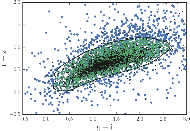
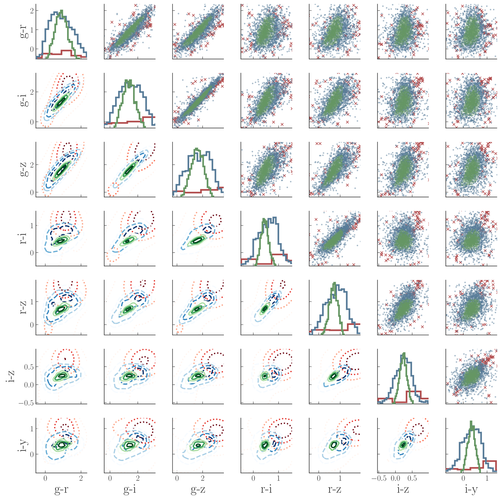
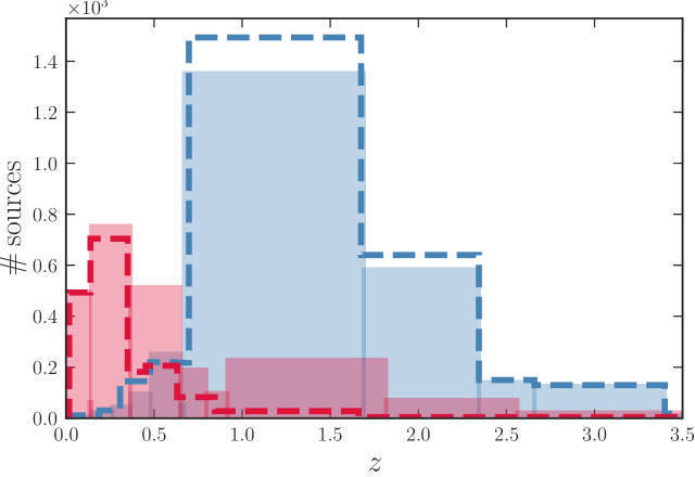
Figure 2 shows the redshift distributions for the SDSS (solid histogram) and Pan-STARRS (open, dashed histogram) five filters training samples, divided in extended (red) and point-like (blue) sources. The overall distribution of both samples is quite similar, with the majority of sources below $z\sim 3$. The main difference is in how extended and point-like objects are distributed. Most extended sources of the Pan-STARRS training sample show $z\lesssim 1$, while we find a non-negligible number of extended sources in the SDSS training sample between $1\lesssim z\lesssim 2$.

Figure 3 presents the r magnitude, g$-$r, J$-$H and W1$-$W2 colour distributions of the training samples (open histograms) and the ARCHES and XPS full catalogues (solid histograms). Although our training samples are about one magnitude brighter than the application samples, their colour distributions are reasonably well reproduced. As noted by Beck et al. (2017), this is an important factor to obtain reliable photometric redshifts. The only major differences are the peaks at $\mathrm{g-r}\sim 1.5$ and $\mathrm{W1-W2}\sim 0$, which are caused by the underlying population of stars in our application samples (see Sect. 5.2).

For a more quantitative estimation of how well our application samples are covered by their corresponding training samples, we estimated the parameter inTSCS (in Training Sample Colour Space, see Appendix) for each source in our final catalogue: For each possible independent combination of two colours (e.g. g$-$r against z$-$y, W1$-$W2 against u$-$g, etcetera) we did a kernel density estimation (KDE) of the distribution of training sample sources in that colour space, and we estimated the 90% probability contour of the KDE (see e.g. Fig. 4). Sources of the application sample inside this contour are well covered by the training sample (green triangles in Fig. 4). Sources well covered in all possible colour combinations (see Fig. 5) have a true inTSCS value in XMMPZCAT. About $\sim 40-50\%$ of the sources are well covered in all colour combinations, and $\sim 85-95\%$ are well covered in at least one colour-colour combination, depending on the particular training sample. Considering the whole XMMPZCAT, 45% of the sources have a true inTSCS value.

Figure 6: Comparison of photometric redshifts for 3XMM sources with optical counterparts in both SDSS and Pan-STARRS catalogues. Green circles are objects having both photo-z with PS greater than 0.7 (see Sect. 5.1). Darker shades of green show higher density of sources. Grey points are the remaining sources. Red, dashed lines show the limit where $|z_{\mathrm{phot}}^{\mathrm{\scriptscriptstyle PS}}-z_{\mathrm{phot}}^{\mathrm{\scriptscriptstyle SDSS}}|/(1-z_{\mathrm{phot}}^{\mathrm{\scriptscriptstyle PS}})=0.15$.

4.2 Merging ARCHES and XPS results

We found 32 460 X-ray sources with counterparts in both ARCHES and XPS catalogues. In order to build our final catalogue of photometric redshifts, we have to select which photo-z include for these sources. Our merging criterion was as follows: in those cases where the ARCHES photo-z was estimated using the same or more filters than the XPS photo-z, and the SDSS photometry was flagged as clean (see Appendix), we selected the ARCHES photo-z; otherwise the XPS photo-z was included in the final catalogue.

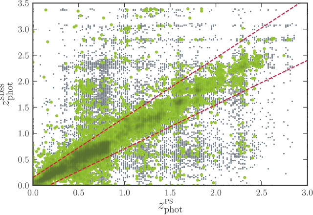
We can use these common sources as a consistency check of our results. If the SDSS and Pan-STARRS counterparts of the X-ray source are in fact the same optical source (i.e. disregarding miss-matching problems), we expect that the photo-z estimated either with SDSS or Pan-STARR photometry should be similar. Figure 6 shows a comparison between the ARCHES and XPS photo-z of these 32 460 common objects. We define that a source has consistent photo-z if $|z_{\mathrm{phot}}^{\mathrm{\scriptscriptstyle PS}}-z_{\mathrm{phot}}^{\mathrm{\scriptscriptstyle SDSS}}|/(1-z_{\mathrm{phot}}^{\mathrm{\scriptscriptstyle PS}})<=0.15$. Using this definition, about 70% of the common sources show consistent photo-z. Restricting the sample to sources having reliable photo-z in both catalogues (i.e. with peak strength equal or greater than 0.7, see Sect. 5.1), the fraction of sources with consistent photo-z is 90% (green circles in Fig. 6).

Figure 7: Spectroscopic against photometric redshifts of SDSS (left) and Pan-STARRS (right) training samples. Blue triangles are point-like sources, red circles are extended sources. Darker shades represent a higher density of sources. Red, dashed lines show the adopted limit for catastrophic outliers (see Sect. 5.1).

5 Results

Table 3: Results of the statistical tests using the training+testing samples (Sect. 5.1).

	(1)		(2)		(3)		(4)		(5)		(6)
	SDDS		SDDS-b		SDDS-c		Pan-STARRS		Pan-STARRS-b		Pan-STARRS-c
# filters	$\sigma_{\mathrm{NMAD}}$	$\eta$ (%)	$\sigma_{\mathrm{NMAD}}$	$\eta$ (%)	$\sigma_{\mathrm{NMAD}}$	$\eta$ (%)	$\sigma_{\mathrm{NMAD}}$	$\eta$ (%)	$\sigma_{\mathrm{NMAD}}$	$\eta$ (%)	$\sigma_{\mathrm{NMAD}}$	$\eta$ (%)
Point-like sources
5 (4)	0.076	29	0.089	32	0.132	39	0.138	41	0.135	41	0.168	45
7 (6)	0.064	19	0.072	22	0.082	22	0.088	25	0.087	27	0.096	27
8 (7)	0.057	20	0.059	21	0.069	24	0.074	26	0.067	28	0.087	28
10 (9)	0.049	14	0.049	13	0.059	20	0.062	17	0.069	21	0.069	17
Extended sources
5 (4)	0.071	18	0.061	11	0.091	28	0.063	13	0.078	21	0.072	19
7 (6)	0.057	14	0.048	8	0.057	19	0.038	6	0.047	11	0.039	5
8 (7)	0.054	12	0.051	7	0.063	13	0.052	9	0.058	10	0.056	9
10 (9)	0.046	9	0.043	6	0.051	10	0.036	4	0.041	7	0.037	4

Figure 8: Relative importance of u$-$g (blue circles) and i$-$y (orange crosses) against redshift for the SDSS and Pan-STARRS 5 filters training samples, respectively (see Sect. 5.1). Solid lines and symbols: extended subsamples; open symbols and dashed lines: point-like subsamples.

Figure 9: Statistics for the derivation of photometric redshifts, using the training+testing SDSS samples. Left column plots correspond to a PS-based selection, right column plots correspond to a zConf selection (see Sect. 5.1). First row: percentage of outliers; second row: normalised median absolute deviation; third row: percentage of rejected sources after filtering; fourth row: percentage of rejected sources that are not outliers. Blue circles correspond to ten filters samples (ugrizJHKW1W2), green traingles to seven filters samples (ugrizW1W2), orange crosses to eight filters samples (ugrizJHK), purple squares to five filters samples (ugriz). Solid lines and symbols correspond to extended sources samples, dashed lines and empty symbols to point-like sources samples. Lines are included just for visualisation improvement.

Figure 10: Statistics for the derivation of photometric redshifts, using the training+testing Pan-STARRS samples. All plots and symbols as in Fig. 9.

5.1 Reliability and accuracy of the photometric redshifts

5.1.1 Statistical tests

One of the main problems of photometric redshifts is estimating their accuracy and reliability. In the case of machine learning techniques, we can obtain a fine estimate of the method’s performance, in the statistical sense, through tests using the corresponding training sample.

Each training sample presented in Sect. 4.1 was randomly split in two subsamples of equal size (training+testing). We used the training subsamples to estimate photometric redshifts with TPZ for the testing subsamples, and we compared these results with their corresponding spectroscopic redshifts. To this end we make use of the most widely used statistical indicators, which are the following:

$$x=\Delta(z_{norm}) =\frac{z_{spec}-z_{phot}}{1+z_{spec}},$$ (1)

$$MAD(x) =Median(|x|),$$ (2)

$$\sigma_{\mathrm{NMAD}}(x) =1.4826\times MAD(x),$$ (3)

$$\eta =\frac{N_{outliers}}{N}\times 100,$$ (4)

where $\sigma_{\mathrm{NMAD}}$ is the normalised median absolute deviation (MAD), and $\eta$ is the percentage of catastrophic outliers. A source is considered a catastrophic outlier if $|x|>0.15$.

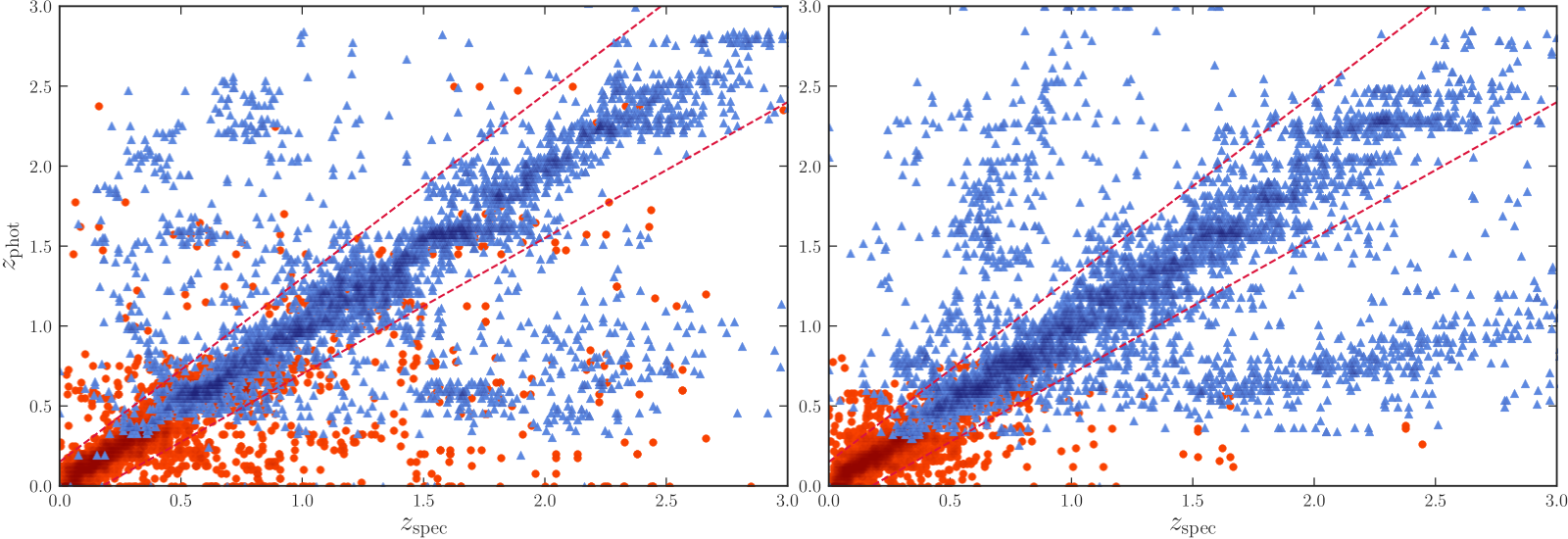
Table 3 (Cols. 1 and 4) shows the results of this test, comparing the performance of SDSS and Pan-STARRS training samples. Figure 7 shows a comparison between spectroscopic and photometric redshifts for SDSS (left) and Pan-STARRS (right) training samples.

Our test show that the Pan-STARRS training sample gets slightly better results for extended sources, but worse for point-like sources, particularly for photometric redshifts estimated using only optical data. It is worth noting that Pan-STARRS training samples for extended sources are a 20-30% smaller, but nevertheless their results are in fact better. The opposite happens with point-like sources: the SDSS training samples are about a 10% smaller, but the performance is better.

We note that this difference in the sizes of the extended and point-like training samples arise from the differences in the redshift distributions of SDSS and Pan-STARRS samples we mentioned above (Fig. 2). Extended sources in Pan-STARRS concentrate below redshift 1, while extended SDSS sources have a non negligible contribution of objects at redshift $\sim 2$. The redshift distribution of the AGN population peaks at redshift two. We can therefore expect that a significant fraction of objects in the SDSS extended samples are AGN-dominated sources. Photometric redshifts for AGN-dominated galaxies are harder to estimate, due to variability effects and their roughly featureless, flat SED (see e.g. Salvato et al., 2009). This could be, partially at least, the reason behind the different performance between training samples. In Pan-STARRS, most AGN-dominated sources are included in the point-like sample, while host-dominated sources concentrates in the extended sample. On the other hand, in the SDSS training samples, AGN- and host-dominated objects are more evenly distributed between extended and point-like samples.

We tested this possibility in two different ways. On one hand, we defined a new set of SDSS training samples (SDSS-b). We used the sources of the original SDSS training samples, but only sources with $z<1$ were included in the extended training samples. The remaining sources were assigned to the corresponding point-like training samples. On the other hand, we again defined a new set of Pan-STARRS training samples (Pan-STARRS-b), but in this case using the SDSS classification to divide the original sample between extended and point-like sources. Then, we repeated again the same test we describe above for these new sets of training samples and estimated the corresponding statistics.

Table 3 (Col. 2 and 5) shows the results for these tests. We can see that removing high redshift sources from the SDSS extended samples does in fact improve its performance, close to the levels of the Pan-STARRS samples, or even better in some cases. The same effect is seen in the Pan-STARRS-b samples: the addition of high-$z$ objects to the extended samples indeed worsen the performance, although they are still better than the SDSS extended samples, except for the five filters sample.

However, this effect does not explain the poorer performance of the Pan-STARRS point-like samples. Both SDSS-b and Pan-STARRS-b point-like samples show a slightly worse performance with respect to the original samples, but SDSS-b still obtained significantly better results.

Another significant difference between SDSS and Pan-STARRS training samples is the set of optical filters. To estimate how the presence of the u and y filters could affect the derivation of photometric redshifts, we defined two new sets of training samples (SDSS-c and Pan-STARRS-c), but using only the common filters between the SDSS and Pan-STARRS surveys (g, r, i, z). Then again, we repeated the same test by randomly splitting the samples in equal-sized training+testing samples. The results are presented in Table 3 (Cols. 3 and 6).

The effect of removing one optical filter in sources with NIR and/or MIR data is not very significant, obtaining similar results in accuracy and fraction of catastrophic outliers. For sources with only optical data the effect is more profound, particularly for the SDSS training sample. The Pan-STARRS sample still shows a better performance for extended sources, while the SDSS sample is better for point-like sources, although the differences in performance between both training samples are greatly reduced.

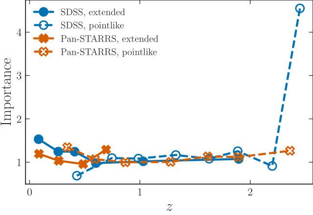
In principle, the relevance of each filter for the estimate of photometric redshifts can be highly dependant on the true redshift of the source. Among the ancillary products of TPZ there is an estimation of the relative importance of each attribute used to calculate the photometric redshifts. Figure 8 shows the importance values we obtained for the u$-$g and i$-$y colours in our test using, respectively, the SDSS and Pan-STARRS five filters training samples. An importance near one means that the redshift information obtained through that particular colour is low compared with the rest of the colour set. This result shows that the y filter is relatively unimportant for the photometric redshifts in the Pan-STARRS sample, as the result of our previous test already suggested. It also shows how relevant is the u filter for sources with redshift above two.

Hence, this could explain, at least partially, the poorer performance of the Pan-STARRS training sample for point-like sources. As discussed above, this subsample contains a high fraction of high redshift sources, and therefore the lack of the u filter here can severely affects the calculation of photometric redshifts.

5.1.2 PDF-based tests

Since TPZ gives the full PDF for the photometric redshift in the predefined redshift space, we can obtain more information on the reliability of the derived redshift for each particular source (see Carrasco Kind & Brunner, 2013; Jones & Singal, 2017). An unimodal PDF, narrowly concentrated around its maximum is a sign of a reliable redshift estimate, while a multi-modal PDF with several local maxima of similar height is a clear sign that the redshift is badly determined.

We calculated several PDF-derived parameters and we tested how a selection of sources based on these parameters affects the statistics in our photo-z derivation. These parameters are defined as follows:

• zConf: The integral of the PDF in the interval $\pm(1+z_{\mathrm{phot}})\times rms$, centred in $z_{\mathrm{phot}}$. $z_{\mathrm{phot}}$ is the mode of the PDF (the absolute maximum and the value chosen as the photometric redshift of the source) and $rms$ is the intrinsic dispersion of the method, which depends on the employed training sample. For our sample we have used $rms=0.06$ and it correspond to the root mean square of the out of bag results given by TPZ (see Carrasco Kind & Brunner 2013). A high value of zConf means that the PDF is highly concentrated around $z_{\mathrm{phot}}$.

• Npeaks: Number of local maxima (peaks) in the PDF.

• PS (Peak strength): 1-P2/P1, where P1 is the probability density of the highest local maximum in the PDF, and P2 is the second maximum peak. If the PDF is unimodal (P2=0) or P2$\ll$P1, $\mathrm{PS}\simeq 1$.

Figure 11: Colour-colour plots of point-like XPS sources showing our separation between stars and no-stars using the hdbscan clustering algorithm (see Sect. 5.2). Left: g$-$z versus z$-$W1. Right: g$-$z versus J$-$K. Green triangles are sources classified as stars; blue circles are sources classified as no stars; grey asterisks show unclassified objects. Darker shades mean a higher density of sources.

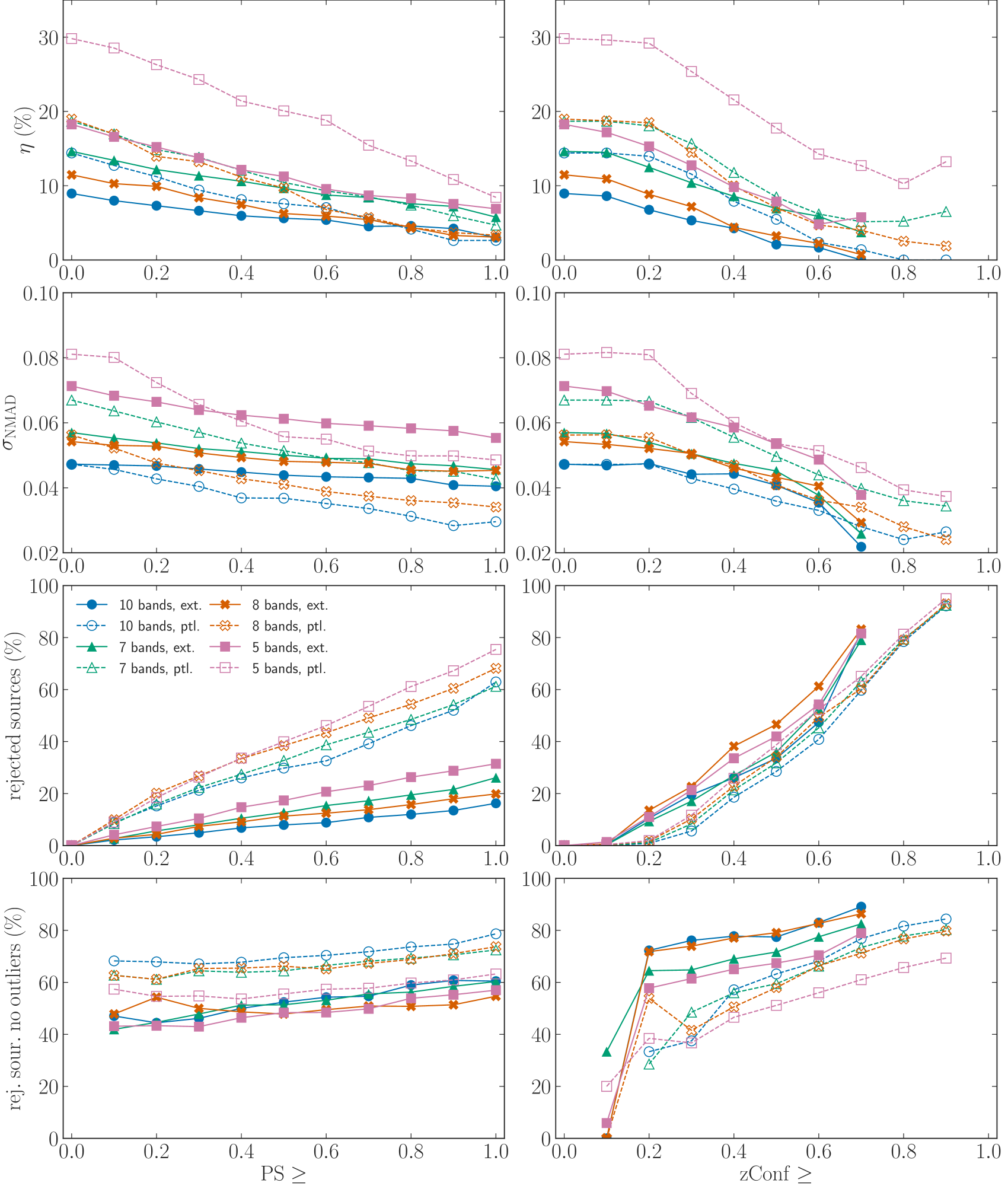
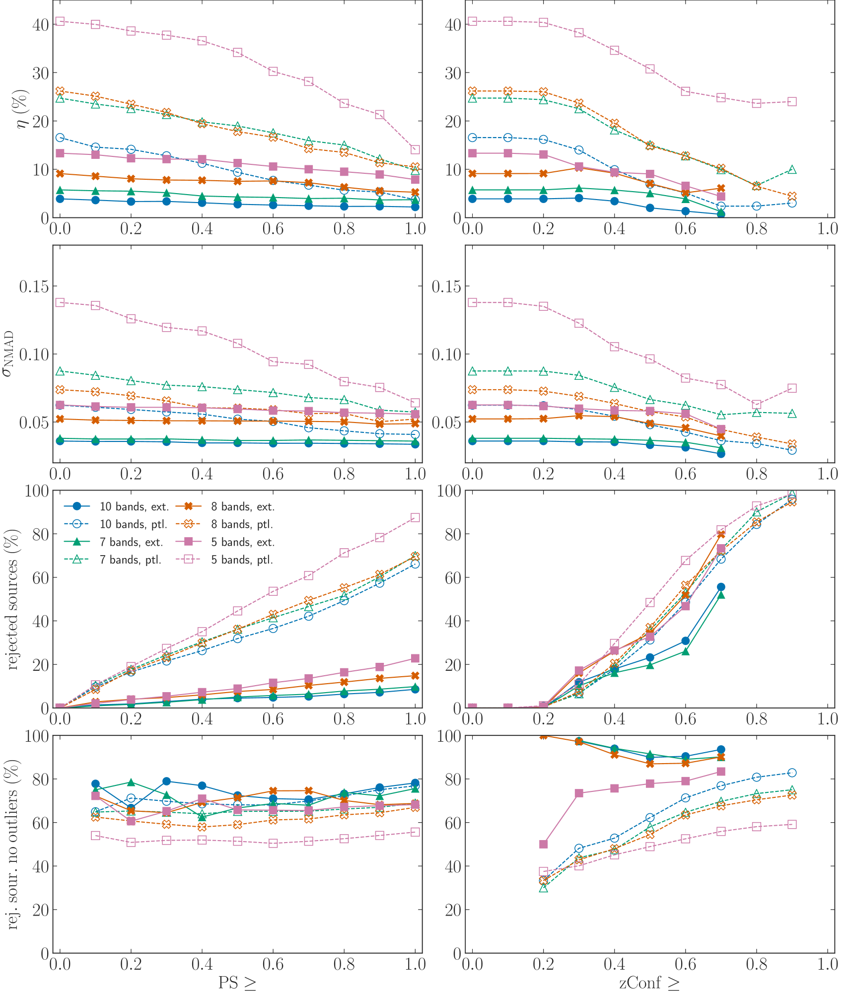
Figures 9 and 10 present the results of our statistical tests using the training+testing samples we described above, for the SDSS and Pan-STARRS samples, respectively. For each sample, we selected sources with PS (left column) or zConf (right column) greater or equal than a given value, and we calculated the percentage of outliers, the normalised median absolute deviation, the percentage of rejected sources with respect to the total number of sources in the full sample (i.e. without any filtering), and the percentage of rejected sources that are not outliers with respect to the number of rejected sources. Npeaks is one if PS is one, therefore an Npeaks-based selection (Npeaks=1) is equivalent to selecting sources with PS=1.

There is an obvious trade-off between selecting high confidence photometric redshifts and the final number of sources in the sample. Finding a compromise between these two factors is therefore necessary.

In the case of SDSS sources, our results show that a percentage of outliers below 10% can be obtained for all but one samples, selecting sources with $\mathrm{PS}\geq 0.6$ or $\mathrm{zConf}\geq 0.5$. For the five filters point-like sample both selections obtain a percentage of outliers about 20%. The values of $\sigma_{\mathrm{NMAD}}$ are in both cases between 0.03 and 0.06, with slightly lower values for the zConf selection. The zConf selection also gives lower percentages of outliers, but the fraction of rejected sources is significantly higher for extended sources. With $\mathrm{PS}\geq 0.6$, about 10-20% of extended sources are rejected, while imposing $\mathrm{zConf}\geq 0.5$ rejects about 30-50%. In both cases the percentage of rejected point-like sources is about 30-40%.

For Pan-STARRS sources we found that a selection with $\mathrm{PS}\geq 0.7$ or $\mathrm{zConf}\geq 0.5$ obtains a percentage of outliers below 10% for extended sources and below 15% for point-like sources. The values of $\sigma_{\mathrm{NMAD}}$ are between 0.03 and 0.07 in both cases. The exception is the 5-filters point-like sample, with $\eta\sim 30\%$ and $\sigma_{\mathrm{NMAD}}\sim 0.09$. Although the percentage of outliers for this sample is still high, applying a quality filter significantly reduces this percentage. Again, the zConf selection gives a slightly lower percentage of outliers, but with a significant higher loss of extended sources. With $\mathrm{PS}\geq 0.7$ the percentage of rejected sources is less than 20% for extended sources and about 40-60% for point-like sources. With $\mathrm{zConf}\geq 0.5$ the fraction of rejected point-like sources is similar, but it reaches 30-50% for extended sources.

Note also that by imposing a quality cut we got a significant lose of sources that are not outliers (see the last row panels of Figs. 9 and 10). For the case of a PS selection, the fraction of rejected not-outliers is between 40 and 80%, depending on the particular subsample, but it remains roughly constant in spite of the selected PS value. On the other hand, the fraction for a zConf-based selection is much more dependant on the selected zConf value, varying between $\sim 20$ and 90%.

Both PS and zConf values are included in our final catalogue, but we did not apply any quality selection based on these parameters. It is up to the final users to find a compromise value that is best suited for their particular scientific goals.

5.2 Identification of stars

At the average X-ray flux levels of the 3XMM catalogue and high galactic latitudes, the expected percentage of X-ray emitting stars is small, below 10%, but not negligible (Barcons et al., 2007). TPZ can be used also to classify sources, and it has in fact been used before to separate optical stars from quasars with an extremely high efficiency by using SDSS and WISE photometry (Carrasco et al., 2015).

As mentioned in Sect. 4, TPZ includes the option of using classification trees while generating the random forest. We can therefore use TPZ with a training sample where the sources were classified in different categories. The number of possible categories is in principle arbitrary, but for our case of star identification we can simply use two values: one if the source is a star and zero if the source is not a star. The properties of this training sample (in our case, photometric colours) can be used to build classification trees and a random forest in a way similar to that presented in Sect. 4. The resulting random forest can then be applied to different samples to separate sources between stars and no stars.

Our first approach for identifying stars in XMMPZCAT was building a training sample of X-ray emitting stars with SDSS data. To this end, we retrieved the ROSAT all-sky survey and SDSS sample of X-ray emitting stars (RASSDSSTAR; Agüeros et al., 2009). However the size of the sample we were able to build using RASSDSSTAR was quite low, $\sim$ 700 sources, and this number was even lower for sources with Pan-STARRS data ($\lesssim 500$).

Hence we used a different approach. Stars are easily separated from galaxies and QSO using a combination of optical and IR colours (see e.g. Wu et al. 2012). The dust content of most stars is low, so it is expected that most stars show lower IR colours (e.g. z$-$W1 or J$-$K) than galaxies or QSO. We can use the objects included in our cross-matched catalogues (ARCHES or XPS) having IR photometry for selecting X-ray emitting stars through colour-colour plots.

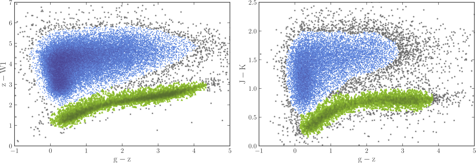
In the ARCHES (XPS) sample we have 16 321 (50 614) point-like sources with the needed optical and IR colours. Figure 11 shows two colour-colour plots for XPS objects. On the left we plotted g$-$z versus z$-$W1 and on the right g$-$z versus J$-$K. As expected, stars are located in the lower region of the plots. For a systematic separation between stars and galaxies/QSO we applied HDBSCAN* (Campello et al., 2013), a hierarchical, density-based clustering algorithm, as implemented in the python package hdbscan (McInnes et al., 2017).

Figure 12: r$-$i versus g$-$z colour-colour plot of point-like XPS sources. Magenta open circles are sources identified as stars using TPZ. Green triangles are sources classified as stars using colour criteria (Fig. 11). Grey solid circles are the remaining point-like objects in the Pan-STARRS sample. Darker shades mean a higher density of sources.

We run hdbscan for each colour-colour plot presented in Fig. 11, dividing the sample between stars (green triangles) and galaxies/QSO (blue circles). Grey asterisks are sources that remained unclassified using the hdbscan algorithm. We imposed a minimum cluster size of 100 objects, and we kept the rest of parameters of the algorithm at the default values.

In order to build our training sample for TPZ, we selected as stars objects identified as stars using NIR or MIR colours, and as no-stars objects identified as galaxies/QSO in NIR and MIR colours. Applying these criteria we build a training sample of 2816 stars and 10 992 no-stars for the ARCHES sample, and of 5555 stars and 36 004 no-stars for the XPS sample.

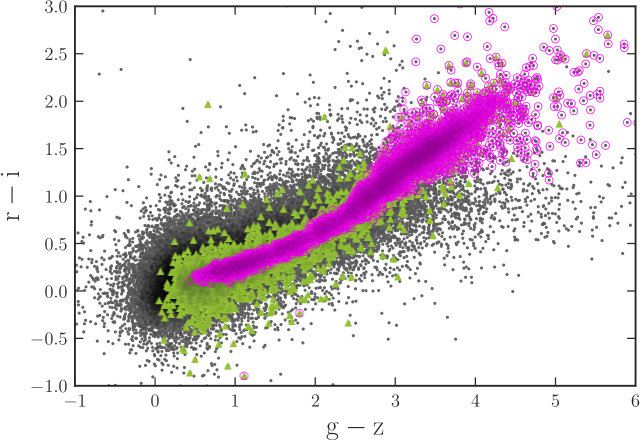
Using these training samples in TPZ we can identify stars for those sources with only optical colours available. For the ARCHES (XPS) sample TPZ identified 4680 (5636) objects as stars, 2008 (1599) of them not identified through the IR-colour selection. In the final catalogue of 100 178 X-ray sources there are 10 830 stars ($\sim 11\%$), after combining those stars identified through IR colours and those identified using TPZ. Figure 12 shows an optical colour-colour diagram for point-like Pan-STARRS sources. The plot clearly shows that, using our training sample, TPZ is able to identify the typical star tail in this kind of diagrams (magenta open circles).

We used this information to flag sources as stars in XMMPZCAT (see Appendix). We included those sources that were identified as stars using their IR colours and the hdbscan algorithm, and those identified through their optical colours using TPZ.

Figure 13: Normalised redshift distributions of XMMPZCAT sources. Left: Full catalogue, with no filtering. Right: Sources with peak strength greater or equal than 0.7 (see Sect. 5.1) and not classified as stars (see Sect. 5.2). The filled histogram shows the normalised distribution using the most probable redshift (the mode) for each source. Lines show the probability density of the sample estimated by adding all the corresponding PDFs. Red lines correspond to extended sources, blue lines to point-like sources. Solid lines represent ARCHES samples, dashed lines the Pan-STARRS samples. Dotted, black line represents the whole sample.

Figure 14: X-ray properties of XMMPZCAT sources (red, hatched histogram), compared with the total population of 3XMM sources in the XMMPZCAT footprint (black, solid line) and the population of 3XMM sources in the XMMPZCAT footprint but with no estimated photo-z (blue, solid histogram). Left: Normalised 0.2-12 keV flux distributions. Right: Normalised hardness ratio (HR2) distributions.

5.3 Properties of XMMPZCAT sources

In this section we present some of the global properties of XMMPZCAT sources, such as redshift, X-ray flux and hardness ratio distributions.

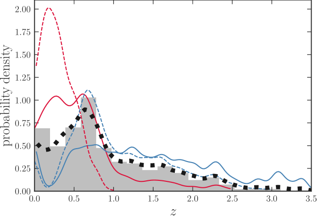
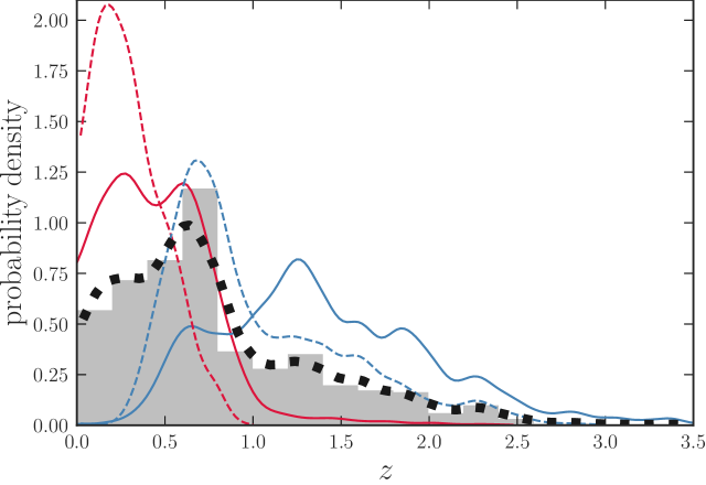
Figure 13 shows the redshift distribution before (left) and after (right) filtering by PDF peak strength (PS$\geq 0.7$), for the full catalogue (black dotted lines) and for each subsample: extended or point-like (red or blue lines), and ARCHES or XPS (solid or dashed lines). We estimated the distributions by adding the TPZ-estimated PDF of each source in the catalogue. For comparison, we also plotted the total redshift distribution estimated using the final photo-z values (the PDF’s mode) included in the catalogue (grey histogram).

Our results show that most XMMPZCAT sources are concentrated below redshift $\sim 1$, with a strong peak at $z\sim 0.7$ and a long tail up to redshift $\sim 2.5$. XPS extended sources show a strong peak at $z\sim 0.2$, with no significant contribution for redshifts greater than 1. Most XPS point-like objects accumulate between redshift 0.3 and 1, with a strong peak at $z\sim 0.7$, a small hump at $z\sim 1.3$ and a long tail up to redshift 2.5.

On the other hand, as discussed in Sect. 4.1, SDSS can detect extended sources at higher redshifts, and hence ARCHES samples show a different distribution between extended and point-like sources. The redshift distribution of the ARCHES extended sample show two peaks at $z\sim 0.2$ and $\sim 0.7$. ARCHES point-like sources are more abundant at higher redshifts than XPS point-like objects, with a peak around $\sim 1.3$ and broadly distributed between redshift $\sim 0.5$ and $\sim 2.5$.

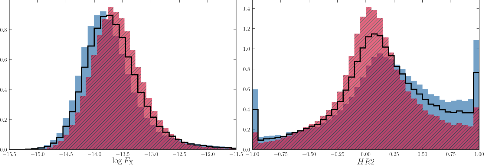
Figure 14 shows the 0.2-12 keV flux (left) and hardness ratio (right) distributions for the XMMPZCAT (red histogram). For comparison we have also included two samples of 3XMM sources in the XMMPZCAT footprint: the black solid line shows the distribution for all 3XMM sources in the footprint and the blue histogram shows only those with no estimated photo-z. We used the hardness ratio between 0.5-1 and 1-2 keV as given in the 3XMM catalogue (HR2, see Rosen et al., 2016). If a source has a hardness ratio close to one, it means that its X-ray emission is larger at high energies than at low energies. Since low energies are more sensitive to X-ray absorption, high hardness ratios are usually understood as a sign of obscuration (see e.g. Severgnini et al., 2012).

The distribution of XMMPZCAT objects is skewed towards higher X-ray fluxes, compared with the total 3XMM population. The median X-ray flux for XMMPZCAT sources is $2.4\times 10^{-14}\leavevmode\nobreak\ \mathrm{erg\,s^{-1}\,cm^{-2}}$ and $1.6\times 10^{-14}\leavevmode\nobreak\ \mathrm{erg\,s^{-1}\,cm^{-2}}$ for 3XMM sources with no photo-z. A Kolmogorov-Smirnov test shows that these distributions are different with $\gg 5\sigma$ confidence.

XMMPZCAT sources seem to present a softer X-ray spectral shape. The hardness ratio distribution is skewed towards lower HR2 values, with a median of 0.08, while 3XMM sources with no photo-z show a median of 0.2. There is a clear under-abundance of XMMPZCAT sources with high hardness ratios compared with the total 3XMM population.

Higher X-ray fluxes and softer spectral shapes suggest that, on average, XMMPZCAT sources could show a lower X-ray obscuration than the global 3XMM population. Although a more detailed analysis of the X-ray properties of these objects would be interesting, this is probably just a selection effect, since we are looking for X-ray sources with counterparts with good photometry.

6 Conclusions

We presented XMMPZCAT, a catalogue of photometric redshifts for XMM-Newton serendipitous X-ray sources. Using TPZ, a machine learning algorithm based on decision trees and random forest, and the training sample presented in Mountrichas et al. (2017), we estimated photometric redshifts for 100 178 objects in the 3XMM-DR6 catalogue outside the Galactic plane. The base of our photo-z estimations is optical photometry from the SDSS and Pan-STARRS catalogues, with additional photometry in the NIR (2MASS, UKIDSS, VISTA-VHS) and MIR (AllWISE) bands if available. XMMPZCAT contains photo-z for about 50% of the X-ray sources within the XMM-Newton observations selected to build the catalogue.

We tested the reliability and accuracy of these photo-z using statistical tests based on the training samples. We found that the accuracy of our results is highly dependent on the number of available filters and the extension (i.e. if the optical counterpart is extended or point-like) of the source. The fraction of outliers range between 4% (9%) for extended Pan-STARRS (ARCHES) sources with 10 available filters, up to 40% (30%) for point-like Pan-STARRS (ARCHES) objects with only optical photometry.

We defined three parameters (PS, zConf, Npeaks) that describe the overall shape of the photo-z PDF for each source. These parameters show how reliable is the estimated photo-z. We found that a selection of sources such as PS¿0.6 significantly reduced the fraction of outliers, particularly for point-like objects. However, no filtering based on this kind of quality criteria was applied in the final version of XMMPZCAT. We included our estimates of this parameters in the catalogue, and is up to the final user to apply the quality selection best suited for the pursued scientific goals.

We also identified the content of stars in the catalogue. We build a training sample of IR colour-selected stars and used TPZ to identify stars among objects with only optical colours. We found that about 10% of the sources are stars, a result consistent with other high Galactic latitude X-ray surveys .

Our results show that most XMMPZCAT sources are concentrated below redshift $\sim 1$, with a strong peak at $z\sim 0.7$ and a long tail up to redshift $\sim 2.5$. They seem to be, on average, slightly brighter in X-rays and with a softer X-ray spectral shape than the total population of 3XMM sources (most probably a selection effect because of searching for counterparts with good photometry).

XMMPZCAT can nevertheless be improved in the future. The size of the catalogue can grow with future versions of 3XMM and the release of new, deeper large area optical surveys. We will also be able to increase the accuracy and reliability of the photo-z: for example by assembling larger training samples, by improving our cross-matching techniques including the photometric data (Salvato et al., 2018) or through variability corrections (Wolf et al., 2004) using the Pan-STARRS multi-epoch information. The latest version of the catalogue is always available in the web site of this project.

XMMPZCAT is a key step to the full exploitation of the scientific potential of the 3XMM catalogue. Thanks to the distance information we have derived, we can improve other 3XMM added-value products. For example, using photometric redshifts along XMMFITCAT we can derive important properties of X-ray sources like X-ray luminosity, temperature of the hot emitting plasmas, rest-frame obscuring column densities and rest-frame energies of emission and absorption features.

Appendix: Description of XMMPZCAT

XMMPZCAT consists of a FITS table with one row for each unique X-ray source, and 17 columns containing the estimated redshift plus additional information about the X-ray source, the optical counterpart and several parameters that can help assessing the reliability of the derived photometric redshift. Not available values are represented by a “null” value. The columns of this table correspond to:

• XMM_SRCID: Source identification number as in 3XMM-DR6.

• XMM_RA, XMM_DEC: X-ray source coordinates as in 3XMM-DR6.

• XMMFITCAT: True if the source is in the XMMFITCAT.

• XMATCH: Origin of the optical counterpart (SDSS-ARCHES or Pan-STARRS).

• proba_XMATCH: Probability that all counterparts are associated with the same real source, as estimated by xmatch.

• opt_SRCID: Source identification number in SDSS-DR13 or Pan-STARRS-DR1.

• Nfilters: Number of photometric data used.

• extended: True if the sources is extended in SDSS-DR13, false if it is point-like.

• ph_flag: Quality of the photometric data (see note below).

• inTCS (in Training Colour Space): True if all colours used to calculate the photometric redshift are inside the colour space well covered by the corresponding training sample.

• STARS: True if the source was identified as a star. It includes both sources identified using IR colours and hdbscan, and optical colours and TPZ.

• SPEC_Z: Spectroscopic redshift in SDSS-DR13 (null if not available).

• PHOT_Z: Derived photometric redshift.

• PHOT_ZERR: One-sigma error of the derived photometric redshift.

• PHOT_ZCONF: Confidence of the photometric redshift. It gives an idea about how narrowly concentrated is the redshift probability distribution (PDF) around PHOT_Z.

• Npeaks: Number of local maxima (peaks) in the PDF.

• PS (Peak Strength): $1-P2/P1$, where $P1$ is the probability density of the highest local maximum in the PDF, and $P2$ is the second maximum peak.

• PHOT_Z2: redshift position of $P2$.

Note on ph_flag. The values of this column have a three character format, XYZ, where X is the flag for optical data, Y for WISE data and Z for NIR data (2MASS, UKIDSS or VISTA). The quality of the data was obtained from the corresponding flags of the respective catalogues. The possible values for X/Y/Z are:

• A: all magnitudes in this range are flagged as good.

• B: some magnitudes in this range have bad photometry.

• F: all magnitudes are bad.

• 0: no photometric data in this range.

In addition, a supplementary FITS table is provided, containing the estimated probability density distribution for the photometric redshift of each source. Both tables can be downloaded from the web site of the project.

References

- Abdalla et al. (2011) Abdalla, F. B., Banerji, M., Lahav, O., & Rashkov, V. 2011, MNRAS, 417, 1891
- Agüeros et al. (2009) Agüeros, M. A., Anderson, S. F., Covey, K. R., et al. 2009, ApJS, 181, 444
- Ahn et al. (2012) Ahn, C. P., Alexandroff, R., Allende Prieto, C., et al. 2012, ApJS, 203, 21
- Albareti et al. (2017) Albareti, F. D., Allende Prieto, C., Almeida, A., et al. 2017, ApJS, 233, 25
- Ball et al. (2008) Ball, N. M., Brunner, R. J., Myers, A. D., et al. 2008, ApJ, 683, 12
- Ball et al. (2007) Ball, N. M., Brunner, R. J., Myers, A. D., et al. 2007, ApJ, 663, 774
- Barcons et al. (2007) Barcons, X., Carrera, F. J., Ceballos, M. T., et al. 2007, A&A, 476, 1191
- Beck et al. (2016) Beck, R., Dobos, L., Budavári, T., Szalay, A. S., & Csabai, I. 2016, MNRAS, 460, 1371
- Beck et al. (2017) Beck, R., Lin, C.-A., Ishida, E. E. O., et al. 2017, MNRAS, 468, 4323
- Benítez (2000) Benítez, N. 2000, ApJ, 536, 571
- Bianchi et al. (2014) Bianchi, L., Conti, A., & Shiao, B. 2014, Advances in Space Research, 53, 900
- Bolzonella et al. (2000) Bolzonella, M., Miralles, J.-M., & Pelló, R. 2000, A&A, 363, 476
- Brammer et al. (2008) Brammer, G. B., van Dokkum, P. G., & Coppi, P. 2008, ApJ, 686, 1503
- Breiman (2001) Breiman, L. 2001, Mach. Learn., 45, 5
- Breiman et al. (1984) Breiman, L., Friedman, J. H., Olshen, R. A., & Stone, C. J. 1984, in Statistics/Probability Series (Belmont, California, USA: Wadsworth Publishing Company)
- Brusa et al. (2010) Brusa, M., Civano, F., Comastri, A., et al. 2010, ApJ, 716, 348
- Budavári & Szalay (2008) Budavári, T. & Szalay, A. S. 2008, ApJ, 679, 301
- Campello et al. (2013) Campello, R. J. G. B., Moulavi, D., & Sander, J. 2013, in Advances in Knowledge Discovery and Data Mining (Springer Berlin Heidelberg), 160–172
- Carrasco et al. (2015) Carrasco, D., Barrientos, L. F., Pichara, K., et al. 2015, A&A, 584, A44
- Carrasco Kind & Brunner (2013) Carrasco Kind, M. & Brunner, R. J. 2013, MNRAS, 432, 1483
- Caruana et al. (2008) Caruana, R., Karampatziakis, N., & Yessenalina, A. 2008, in Proceedings of the 25th International Conference on Machine Learning, ICML ’08 (New York, NY, USA: ACM), 96–103
- Casali et al. (2007) Casali, M., Adamson, A., Alves de Oliveira, C., et al. 2007, A&A, 467, 777
- Chambers et al. (2016) Chambers, K. C., Magnier, E. A., Metcalfe, N., et al. 2016, ArXiv e-prints [arXiv:1612.05560]
- Collister & Lahav (2004) Collister, A. A. & Lahav, O. 2004, PASP, 116, 345
- Corral et al. (2015) Corral, A., Georgantopoulos, I., Watson, M. G., et al. 2015, A&A, 576, A61
- Cross et al. (2012) Cross, N. J. G., Collins, R. S., Mann, R. G., et al. 2012, A&A, 548, A119
- Cutri et al. (2003) Cutri, R. M., Skrutskie, M. F., van Dyk, S., et al. 2003, 2MASS All Sky Catalog of point sources. (The IRSA 2MASS All-Sky Point Source Catalog, NASA/IPAC Infrared Science Archive.)
- Cutri et al. (2013) Cutri, R. M., Wright, E. L., Conrow, T., et al. 2013, VizieR Online Data Catalog, 2328
- De Maesschalck et al. (2000) De Maesschalck, R., Jouan-Rimbaud, D., & Massart, D. L. 2000, Chemometrics and intelligent laboratory systems, 50, 1
- Della Ceca et al. (2004) Della Ceca, R., Maccacaro, T., Caccianiga, A., et al. 2004, A&A, 428, 383
- D’Isanto & Polsterer (2018) D’Isanto, A. & Polsterer, K. L. 2018, A&A, 609, A111
- Doi et al. (2015) Doi, Y., Takita, S., Ootsubo, T., et al. 2015, PASJ, 67, 50
- Epchtein et al. (1994) Epchtein, N., de Batz, B., Copet, E., et al. 1994, Ap&SS, 217, 3
- Esquej et al. (2013) Esquej, P., Page, M., Carrera, F. J., et al. 2013, A&A, 557, A123
- Flewelling et al. (2016) Flewelling, H. A., Magnier, E. A., Chambers, K. C., et al. 2016, ArXiv e-prints [arXiv:1612.05243]
- Fotopoulou et al. (2016) Fotopoulou, S., Pacaud, F., Paltani, S., et al. 2016, A&A, 592, A5
- Georgakakis & Nandra (2011) Georgakakis, A. & Nandra, K. 2011, MNRAS, 414, 992
- Hambly et al. (2008) Hambly, N. C., Collins, R. S., Cross, N. J. G., et al. 2008, MNRAS, 384, 637
- Hewett et al. (2006) Hewett, P. C., Warren, S. J., Leggett, S. K., & Hodgkin, S. T. 2006, MNRAS, 367, 454
- Hsu et al. (2014) Hsu, L.-T., Salvato, M., Nandra, K., et al. 2014, ApJ, 796, 60
- Irwin et al. (2004) Irwin, M. J., Lewis, J., Hodgkin, S., et al. 2004, in Proc. SPIE, Vol. 5493, Optimizing Scientific Return for Astronomy through Information Technologies, ed. P. J. Quinn & A. Bridger, 411–422
- Jones & Singal (2017) Jones, E. & Singal, J. 2017, ArXiv e-prints [arXiv:1709.01576]
- Lahav & Collister (2012) Lahav, O. & Collister, A. A. 2012, ANNz: Artificial Neural Networks for estimating photometric redshifts, Astrophysics Source Code Library
- Lawrence et al. (2007) Lawrence, A., Warren, S. J., Almaini, O., et al. 2007, MNRAS, 379, 1599
- Liu et al. (2016) Liu, Z., Merloni, A., Georgakakis, A., et al. 2016, MNRAS, 459, 1602
- Mahalanobis (1936) Mahalanobis, P. 1936, in Proc. National Institute of Science, India, Vol. 2, National Institute of Science of India, 49–55
- McInnes et al. (2017) McInnes, L., Healy, J., & Astels, S. 2017, The Journal of Open Source Software, 2
- McMahon et al. (2013) McMahon, R. G., Banerji, M., Gonzalez, E., et al. 2013, The Messenger, 154, 35
- Menzel et al. (2016) Menzel, M.-L., Merloni, A., Georgakakis, A., et al. 2016, MNRAS, 457, 110
- Mingo et al. (2016) Mingo, B., Watson, M. G., Rosen, S. R., et al. 2016, MNRAS, 462, 2631
- Motch et al. (2016) Motch, C., Carrera, F., Genova, F., et al. 2016, ArXiv e-prints [arXiv:1609.00809]
- Mountrichas et al. (2017) Mountrichas, G., Corral, A., Masoura, V. A., et al. 2017, A&A, 608, A39
- Pineau et al. (2017) Pineau, F.-X., Derriere, S., Motch, C., et al. 2017, A&A, 597, A89
- Pizzocaro et al. (2016) Pizzocaro, D., Stelzer, B., Paladini, R., et al. 2016, A&A, 587, A36
- Rosen et al. (2016) Rosen, S. R., Webb, N. A., Watson, M. G., et al. 2016, A&A, 590, A1
- Rowan-Robinson et al. (2008) Rowan-Robinson, M., Babbedge, T., Oliver, S., et al. 2008, MNRAS, 386, 697
- Salvato et al. (2018) Salvato, M., Buchner, J., Budavári, T., et al. 2018, MNRAS, 473, 4937
- Salvato et al. (2009) Salvato, M., Hasinger, G., Ilbert, O., et al. 2009, ApJ, 690, 1250
- Scargle et al. (2013) Scargle, J. D., Norris, J. P., Jackson, B., & Chiang, J. 2013, ArXiv e-prints [arXiv:1304.2818]
- Schlafly & Finkbeiner (2011) Schlafly, E. F. & Finkbeiner, D. P. 2011, ApJ, 737, 103
- Severgnini et al. (2012) Severgnini, P., Caccianiga, A., & Della Ceca, R. 2012, A&A, 542, A46
- Skrutskie et al. (2006) Skrutskie, M. F., Cutri, R. M., Stiening, R., et al. 2006, AJ, 131, 1163
- Taylor (2005) Taylor, M. B. 2005, in Astronomical Society of the Pacific Conference Series, Vol. 347, Astronomical Data Analysis Software and Systems XIV, ed. P. Shopbell, M. Britton, & R. Ebert, 29
- The Astropy Collaboration et al. (2018) The Astropy Collaboration, Price-Whelan, A. M., Sipőcz, B. M., et al. 2018, ArXiv e-prints [arXiv:1801.02634]
- Wolf et al. (2004) Wolf, C., Meisenheimer, K., Kleinheinrich, M., et al. 2004, A&A, 421, 913
- Wright et al. (2010) Wright, E. L., Eisenhardt, P. R. M., Mainzer, A. K., et al. 2010, AJ, 140, 1868
- Wu et al. (2012) Wu, X.-B., Hao, G., Jia, Z., Zhang, Y., & Peng, N. 2012, AJ, 144, 49
- Yang et al. (2017) Yang, Q., Wu, X.-B., Fan, X., et al. 2017, AJ, 154, 269
- Zacharias & Gaume (2011) Zacharias, N. & Gaume, R. 2011, in Journées Systèmes de Référence Spatio-temporels 2010, ed. N. Capitaine, 95–100