Synchronization of Conservative Parallel Discrete Event Simulations on a Small-World Network
Abstract
We examine the question of the influence of sparse long-range communications on the synchronization in parallel discrete event simulations (PDES). We build a model of the evolution of local virtual times (LVT) in a conservative algorithm including several choices of local links. All network realizations belong to the small-world network class. We find that synchronization depends on the average shortest path of the network. The time profile dynamics are similar to the surface profile growth, which helps to analyze synchronization effects using a statistical physics approach. Without long-range links of the nodes, the model belongs to the universality class of the Kardar–Parisi–Zhang equation for surface growth. We find that the critical exponents depend logarithmically on the fraction of long-range links. We present the results of simulations and discuss our observations.
I Introduction
Progress in computation hardware in the last decade has been mainly in the direction of multicore/distributed systems. It is a big challenge to use modern hardware effectively, and creating a single program able to orchestrate a huge number of nodes and cores is not trivial joubert2016parallel ; zhu2015high .
Here, we discuss the problem of synchronization within one family of parallel simulations. The class of considered systems comprises very many individual elements interacting asynchronously with each other, and events occur at some discrete instants. Simulating such systems using sequential algorithms requires a vast amount of processing time and memory. The method for simulating systems on parallel/distributed computers, which allows implementing a faithful synchronization, is called parallel discrete event simulation (PDES) fujimoto1990parallel ; fujimoto2016research .
The simulation technique is used in many areas of physics; examples include simulation of granular dynamics richardson2011numerical , kinetic Monte Carlo simulations nilmeier2014rigorous , and simulation of 3D sintering garcia2010parallel . It is proved to work on millions of cores oppelstrup2016spock .
It was shown in korniss2000massively that evolution of the simulated time profile in PDES is analogous to the evolution of nonequilibrium surface growth. A model of the time profile evolution was proposed, and in the case where the processing elements (PEs) communicate only with neighbors, such a model can be mapped on the (1+1)-dimensional Kardar–Parisi–Zhang (KPZ) equation kardar1986dynamic . This finding helps to understand the synchronization problem in the language of statistical physics. For example, (i) the positivity of the profile speed is mapped on the property of deadlock absence, and (ii) the evolution of the profile width, which is described with the KPZ critical exponents, reflects the desynchronization of the PEs. Taking these into account, we mainly use the language of statistical physics instead of computational science in what follows.
Assuming local communication between the PEs restricts the model application to a relatively small number of applications. Generally, long-range communications between processor elements do occur in simulations. It is reasonable to investigate a more realistic link topology.
Here, we consider PDES on small-world (SW) networks watts1998collective . The current state of research with SW networks is presented in Section III. The main topological feature of a SW network is that for relatively small amount of long-range links, the average distance changes from a linear to a logarithmic dependence on the system size newman2010networks . Clearly, this should drastically change the behavior of the whole system. It was found in korniss2003suppressing ; guclu2006synchronization that random long-range links between PEs strongly influence synchronization properties and the scalability of PDES. A synchronization scheme with additional long-range links introduces a relaxation term in the evolution of the virtual time profile. This term implies the absence of large-amplitude long-wavelength modes guclu2006synchronization in the surface. Consequently, the average width of the profile becomes finite, while the average progress rate remains a nonzero constant in the limit of infinite system size. In other words, (i) introducing long-range links does not change the important property of the local conservative algorithm, the deadlock absence; (ii) the long-range links increases the synchronization of simulations. It was also found that the average width in sufficiently large systems is proportional to the correlation length , and , where is the probability of the long-range interactions.
We construct the topology of the communications between PEs in the framework of the SW approach watts1998collective . The concentration of long-range communications is the main parameter in our research. We find that the clustering coefficient value does not qualitatively influence the development of surface growth. The quantitative change of the rate of surface growth and the surface width behavior is independent of the local connectivity. For this, we analyze networks with only nearest neighbors, with nearest and next-nearest neighbors, and so on. We thus find some universal properties. Our main conclusion is that the average length of the network and number of local connections govern the surface growth dynamics. The average length is a function of the parameter and is known to behave logarithmically for values that are not too small. It is important that we do not change the update scheme of the conservative PDES algorithms as in the papers korniss2003suppressing ; guclu2006synchronization . Our purpose is to investigate how the SW topology of the communication links influences the synchronization properties of PDES, i.e., the statistical properties of the surface growth foo1 .
We build our model on two types of SW networks. Both have a small average shortest path (the main criterion of “small-worldness”). One SW realization has a zero clustering coefficient (the second feature of SW networks watts1999small is a nonzero clustering coefficient). We find that the average speed profile decreases slowly as the parameter increases and the speed is always positive. The average profile width becomes finite in the limit of an infinite system size in accordance with the result in guclu2006synchronization . Another new result here is an estimate of the dependence of the growth exponent on the SW parameter : the dependence is logarithmic.
This paper is organized as follows. In section II, we describe the conservative model for PDES korniss2000massively . Section III contains a detailed description and an analysis of SW topologies. In section IV, we describe our one-dimensional SW scheme and present the results. In section V, we analyze the dependence of the measured quantities on the number of local links. In section VI, we summarize our work and discuss the results.
II Basic Conservative PDES scheme
Parallel discrete event simulation is a subclass of parallel simulation where changes in the components of the system from one state to another occur instantaneously. These changes are called events. The system being simulated is divided into disjoint subsystems. Subsystems are processed by PEs, which are hardware dependent and may be a computing node, CPU, core, or thread. In the simplest case, each PE carries only one site of the underlying system (e.g., one spin in a magnetic model). The important feature of PDES is that the PEs communicate with each other asynchronously and via messages. Each PE progresses at its own pace and has its own simulated time, also called the local virtual time (LVT) jefferson1985virtual . Different synchronization schemes are possible for preserving the causality of computations shchur2004evolution . We focus our discussion on a conservative algorithm, which avoids the possibility of any type of causality error by checking every causality relation at each update attempt fujimoto1990parallel .
The model of the time profile evolution regards LVT as Poisson arrivals. In the basic one-dimensional case, the network topology is a ring korniss2000massively , and PEs hence interact only with nearest neighbors. Let be the number of PEs and be the number of parallel steps. The set of LVTs constitutes the virtual time profile. At each time step, only those PEs whose LVTs are not larger than the LVTs of their nearest neighbors may increment their LVTs by an exponentially distributed random value. These PEs are said to be active. Otherwise, if the LVT of a PE is larger than the LVT of some neighbor, this PE is not updated and is said to be passive. The relative amount of active PEs (those simulating system evolution) is called the utilization
| (1) |
and is an important characteristic of the evolution of the LVT profile. The average is taken over many independent realizations. In the basic conservative scheme, the utilization at the given instant is equal to the density of local minima of the profile, . The value of the utilization can be used as a measure of algorithm effectiveness.
The second important observable is the spread or width of the LVT profile, defined as
| (2) |
where is the mean height of the time profile.
As the number of PEs in a parallel architecture increases to hundreds of thousands, a fundamental question of the scalability of the underlying algorithm emerges. To be scalable, a PDES algorithm must have the following properties: (1) the LVT profile should progress on average with a nonzero rate, and (2) the width of the profile should be bounded by a constant as the number of PEs goes to infinity. A PDES algorithm is said to be fully scalable if both conditions are satisfied toroczkai2003virtual . It is interesting that the scalability of computations is defined in the limit of an infinite system size. This is one more analogy with the corresponding physical system for which the thermodynamic limit is reached in the same limit.
We briefly recall the main results of a study of the basic conservative scheme korniss2000massively . The LVT profile width increases with time and then saturates to the steady-state regime after some time . Before saturation, the width grows as , where . In the steady state, the width is stationary and depends on the system size , . The two values of the exponents and are close to those of the KPZ universality class kardar1986dynamic , and . The estimate of the utilization of the algorithm (measure of the algorithm effectiveness) given in shchur2004evolution is . Therefore, the basic conservative algorithm is computationally scalable in one dimension because the average utilization is greater than zero. But the width of the LVT profile diverges as the number of nodes increases, which means that the PEs became less synchronized. Therefore, the conservative PDES algorithm is not fully scalable. In other words, the algorithm is still applicable for any large system (it somehow progresses in time with positive utilization) although it becomes less and less effective as the number of PEs increases because the PEs become more and more desynchronized as the simulation progresses (the width of the time increases with the number of PEs).
III Small-world networks
Small-world networks comprise a class of networks usually characterized by a small average shortest path length and a high degree of clustering. These properties are observed in many real technological, biological, social, and information networks. There is no rigid definition of “small-worldness,” and different criteria for classifying networks into regular, SW, and random classes have been proposed during the last decade watts1999small ; humphries2008network ; barranca2015low ; borassi2015hyperbolicity .
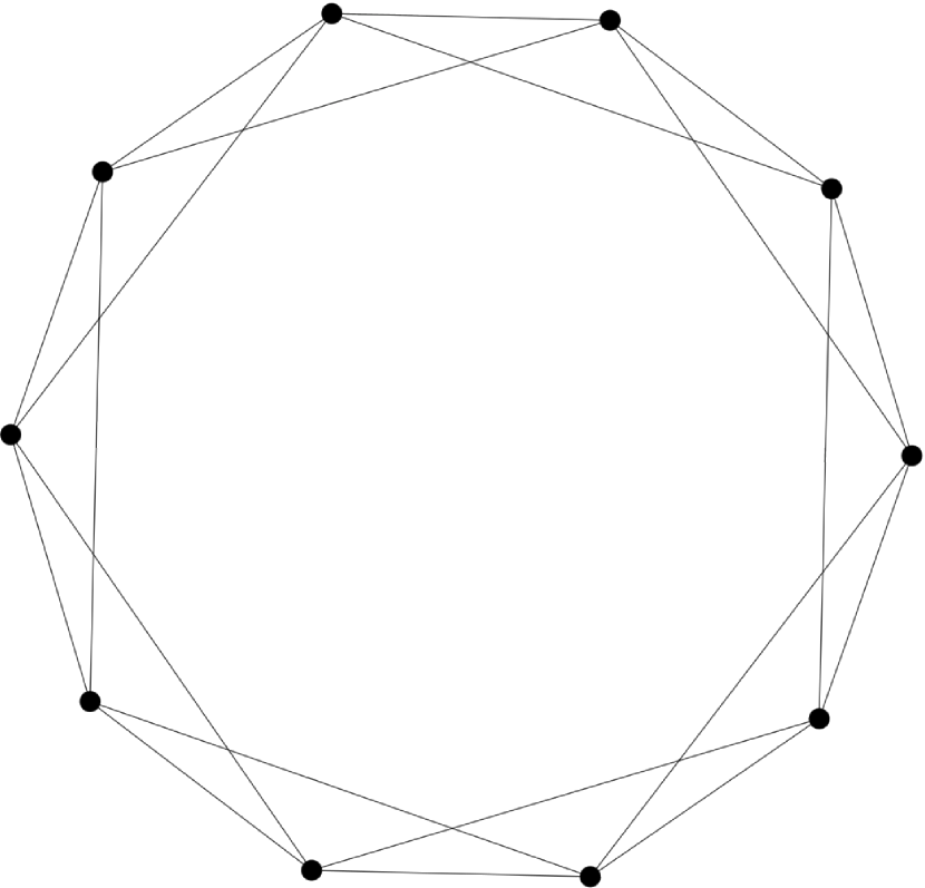
For precision, we first give some basic definitions and notations. We consider a one-dimensional lattice with periodic boundary conditions, where each node is connected with neighbors (Fig. 1a). We call two nodes neighbors if there is an edge between them. The total number of nodes is denoted by . We also need a parameter , which can be interpreted as a degree of randomness. We consider two structural properties of networks, the average shortest path and the clustering coefficient.
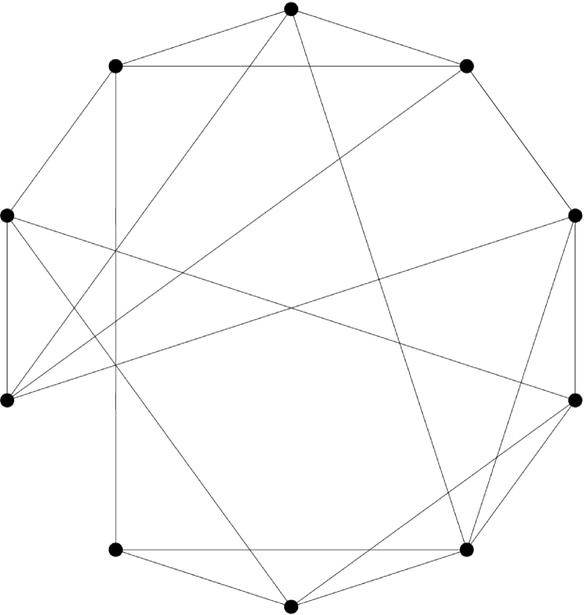
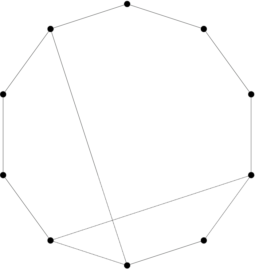
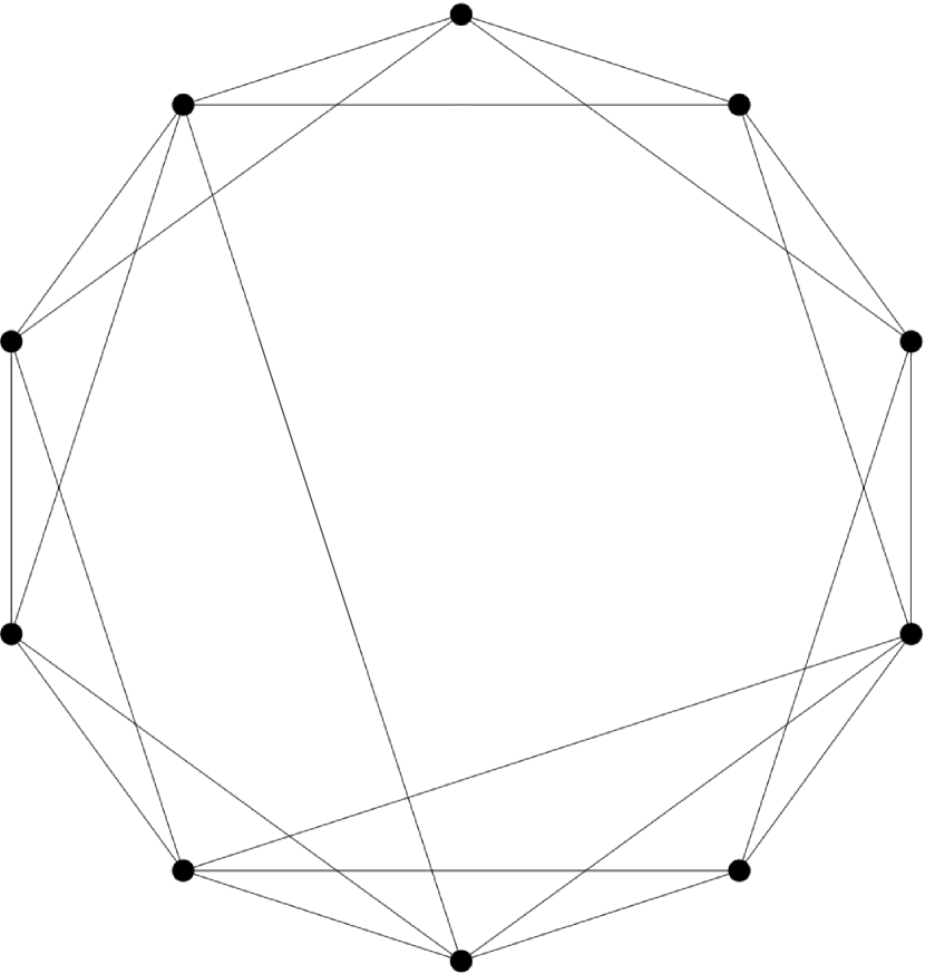
There are several ways to construct networks with long-range links. Given a one-dimensional lattice with each node connected to closest nodes (see Fig. 1a), each edge of the graph is randomly rewired with probability , i.e., one end of the edge is moved to a node chosen at random from the rest of the lattice nodes (see Fig. 1b). Another way to build a network is by adding links with probability above the regular lattice (see Fig. 2).
We conduct our study on three different networks based on both constructions described above. For simplicity, we give a short code names to the networks: “A (add) or R (rewrite) – parameter ”. The construction algorithms are:
-
1.
A–k1. (1) Start with a ring lattice with nodes where each node is connected to its closest nodes. (2) Randomly add exactly edges above the regular lattice (Fig. 2a).
- 2.
-
3.
R–k2. (1) Start with a ring lattice with nodes where each node is connected to its closest nodes. (2) Randomly choose exactly edges and rewrite them randomly (Fig. 1b).
The parameter thus can be regarded as the average number of random long-range links per node.
a)
b)
a)
b)
Average shortest path.
The average shortest path is defined as
| (3) |
where is a chemical distance barrat2000properties , the minimum number of nodes between vertices and .
In regular lattices, the average shortest path grows linearly with the system size:
For the length grows as:
For SW networks, we have the scaling relation newman2000mean ; newman1999renormalization
| (4) |
where is a lattice dimension, is the concentration of long-range links normalized with the number of local connections, and is a universal scaling function,
| (5) |
The above relation indicates a crossover transition between regular and SW networks. The number of rewired or added links () must be small but finite. The regime with is not easily attained in practice for networks of a finite size .
Clustering coefficient.
The clustering coefficient quantifies a “cliquishness” of a network. It is defined as follows. Let be the number of neighbors of a node . Node can have at most possible links between all its neighbors. Let be the actual number of such links. Then the local clustering is , and the clustering coefficient is the average local clustering over all nodes barrat2000properties .
The clustering coefficient of a regular lattice is high: . In contrast, random networks are not clustered: . There are several analytic estimates of the clustering coefficient of SW networks barrat2000properties ; newman2002structure ; watts1999small .
For example, Barrat and Weight barrat2000properties derived expression (6) for the clustering coefficient based on the reasoning that the local clustering coefficient in the SW network remains the same as in a regular lattice if all three edges connecting the node to its two neighbors and the neighbors between themselves are not rewired. This happens with probability :
| (6) |
Watts in his book watts1999small used a more complex analysis of clustering phenomena and derived his expression (7) via the effective local degree and the effective global degree (for more detail, see Chapter 4 in the book watts1999small ):
| (7) |
One more formula is Newman’s newman2002structure equation
| (8) |
In this formula, decreases slowly with and hence remains sufficiently high for a small amount of long-range links (Fig. 3). These three formulas are derived for the SW-networks constructed by rewiring links, it is R–k2 in our case. It is seen from Fig. 3, that clustering coefficient for the network A–k2 follow the formulas only for a very small value of . For a SW network A–k1 with , we have . Adding long-range links increases the probability of a nonzero clustering coefficient in such a network, namely, the clustering coefficient for A–k1.
The informal SW definition at the beginning of this section can now be formulated more precisely: “a SW graph is a large-, sparsely connected, decentralized graph () with a characteristic path length close to that of an equivalent random graph () but with a much greater clustering coefficient ()” watts1999networks .

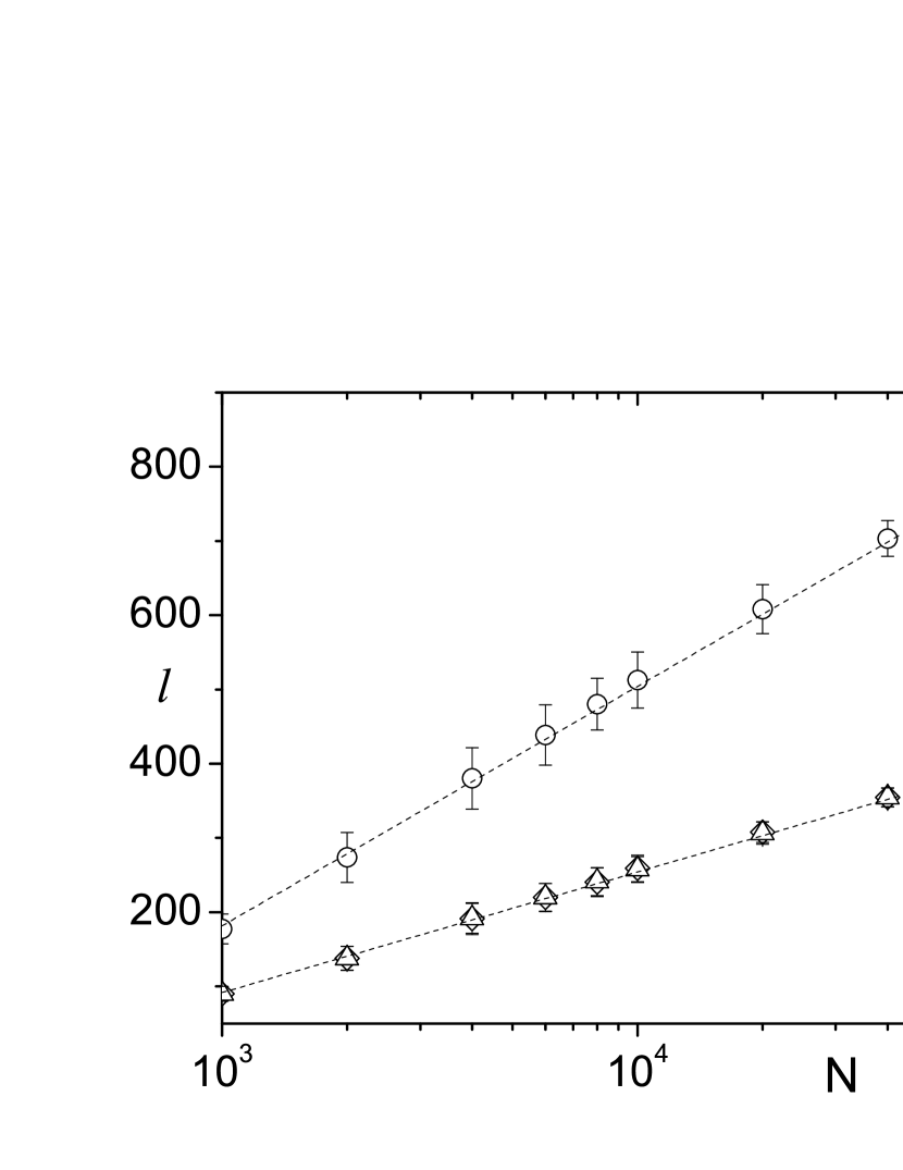
To ensure that the constructed networks are indeed SW networks, we analyze the dependence of the average shortest path length on the parameter and the system size . We find that depends logarithmically on for all for all networks (Fig. 4). Scaling relation (4) is also observed in our data. We plot the average shortest path as a function of the parameter for the network of size , and it is well approximated (see Fig. 5) by
| (9) |
We also calculate clustering coefficients in our models. For the network A–k1, . Strictly speaking, this model does not fully satisfy the criteria for SW networks. For the networks A–k2 and R–k2, we plot and compare the results with different analytic estimates (Fig. 3). The agreement is good for small (), and the clustering coefficient for A–k2 and R–k2 is close to , which equals for .

IV Small-world synchronization scheme
IV.1 Model of time evolution in the conservative algorithm
The key property of the conservative synchronization scheme for PDES is the preservation of causality. In the general case, causality is defined in terms of the dependency matrix with elements , where if the process simulated by PEi depends on PEj, and otherwise. Causality is preserved if the local virtual time (LVT) of PEi is lower than LVT of those PEj on which PEi depends.
The time evolution begins with a flat profile , . To preserve causality, we randomly update those LVTs of PEs that are lower than LVTs of the PEs on which they depend, i.e., using links defined by the dependency matrix . This leads to the rule
| (10) |
where is a random value drawn from the Poisson distribution, is the set of all local times of the PEs connected to PEi by local or long-range communication links, .
As is known, the model on the regular one-dimensional lattice belongs to the KPZ universality class korniss2000massively . This can be seen by the following reasoning. First, we represent Eq. (10) in the form
| (11) |
neglecting long-range links and using the Heaviside step function .
Second, replacing differences between local times with the local slope
| (12) |
we obtain the equation for the density of local minima (or the utilization):
| (13) |
It was shown in krug1990universal that there is a finite-size correction to the growth rate. The finite-size behavior of the average profile speed is
| (14) |
where is the value of the average speed in the asymptotic infinite number of PEs and is the roughness exponent. Equation (14) is confirmed by simulating LVT profile growth. For the KPZ model , while in the model of evolution of the LVT profile, . This is due to nonuniversal short-range correlations between the slopes in the profile.
The average speed depends weakly on the type of distribution of the random variable . For , it was shown in shchur2004evolution that the average speed for a uniform distribution of , for a Gaussian distribution of , and for a Possion distribution of .
It was argued by Korniss et al. korniss2000massively that the coarse-grained slope of the time horizon in the continuum limit is evaluated according to the Burgers equation kardar1986dynamic
| (15) |
and the coarse-grained time profile , satisfies the KPZ equation
| (16) |
which should be extended with noise to capture the fluctuations.
We can expect that the evolution of the time profile belongs to the KPZ universality class. Numerical analysis korniss2000massively ; shchur2004evolution supports this expectation. In the case of long-range links, we can expect deviation from KPZ universality class.
In the case of long-range links, we can rewrite Eq. (11) as
| (17) |
where the product is computed only for long-range links coming from the node PEi, which is denoted by the prime in . The average time profile speed in this case is
| (18) |
where . It is clear from Eq. (18) that additional dependencies decrease the LVT profile speed. In other words, adding long-range links decreases the utilization. Simulations confirm this observation.
IV.2 Simulations
The simulation parameters are the number of PEs, the concentration of long-range links per PE, and the number of discrete simulation steps. The matrix is randomly initialized with one of the construction algorithms described in section III.
The average speed and the average profile width are calculated after each update using the respective expressions (1) and (2). For each set of parameters and , we use 1500 different realizations of the random process running in parallel. The parameter changes from to , and the number of PEs ranges from to .
IV.2.1 Average speed
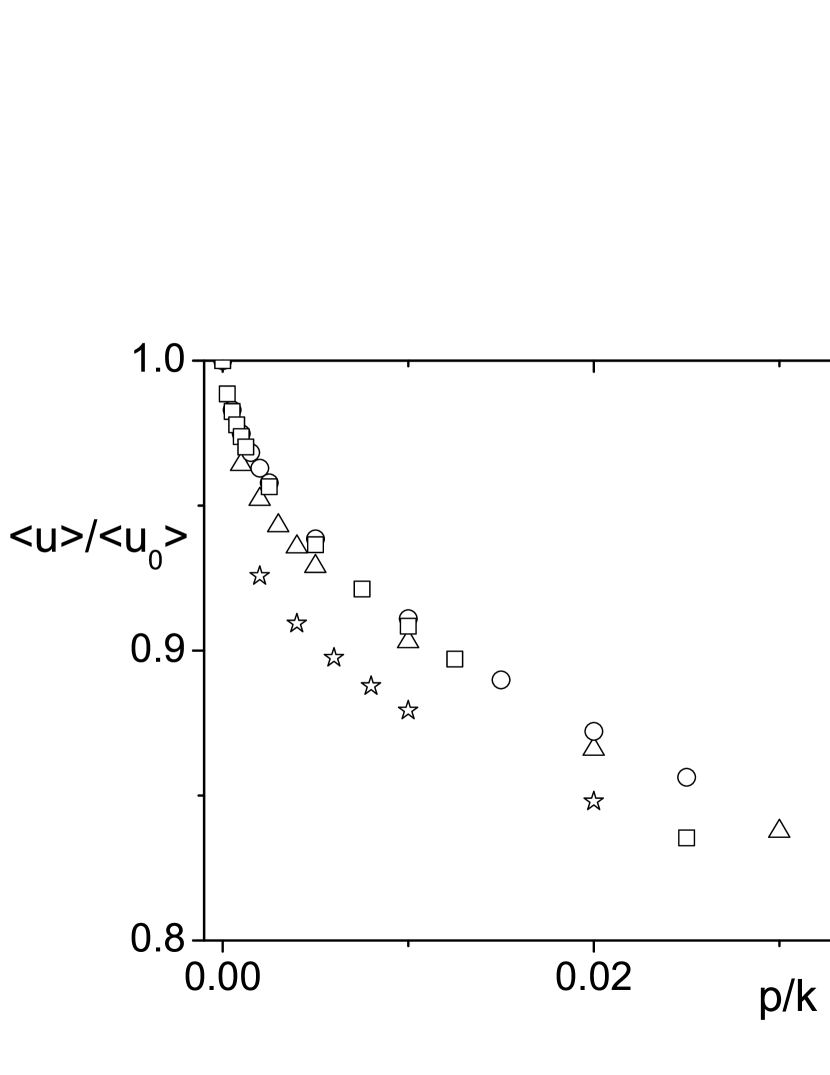
Figure 6 shows the dependence of the average speed on the concentration for three realizations of the SW networks A–k1, A–k2, and R–k2: they are the respective networks with two closest neighbors and randomly added links, with four closest neighbors and randomly added links, and with four closest neighbors and randomly rewired links.

a) A–k1

b) A–k2

c) R–k2
It can be seen in Fig. 6 that the average speed decreases as the concentration increases and is smaller for the networks A–k2, and R–k2 because of the dependence on the next-to-neighbors. Strictly speaking, we should rewrite Eqs. (17) and (18) in this case as
| (19) |
Using Eq. (12), we obtain the expression for the average profile speed on the network A–k2
| (20) |
The presence of next-to-neighbors reduces the average speed , and the average speed for . It can be seen that the speed remains positive for small concentrations , which means that the SW-synchronized simulation scheme maintains a nonzero average utilization. For example, we have in A–k1 for and for . It is seen from Figures 6, that the average speed is hardly different for and .
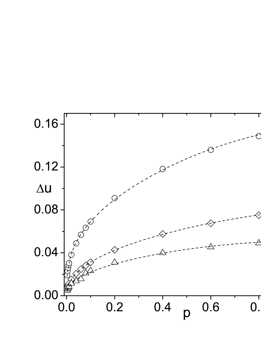
Figure 7 shows the difference of the average speed depending on the SW network realization in the systems of PEs. For small values of the parameter , the difference between the average speed on the network A–k1 and networks A–k2 and R–k2 is significant. This is expected from Eqs. (18) and (20). In the latter equation, the additional terms slow the interface growth speed.
For close to unity, the average speeds on the networks A–k1 and R–k2 are approximately the same. This can be explained by comparing the average amount of dependencies in these networks. For , the network A–k1 has links between the PEs, and the network R–k2 also has links. We can conclude that the average speed of the LVT profile on SW networks mainly depends on the number of links in the communication network.

The dependence of the average speed on the parameter is nonlinear. Let be the difference between the average speed on a SW network and the average speed on a regular lattice:
The difference between the speeds is well approximated by a power-law function (Fig. 8):
| (21) |
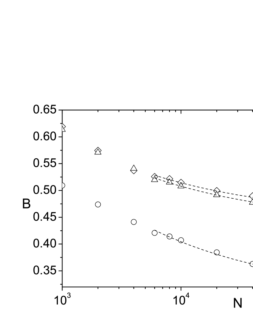
The values of the exponent are given in Table 1. It can be seen from the table that the exponent decreases with the number of PEs. Figure 9 shows the exponent for three SW network realizations. We find the asymptotic behavior of in the limit of a large number of PEs by approximating with the function
| (22) |
In the limit as , the exponent approaches the values for the network A–k1, for the network A–k2, and for the network R–k2.
The behavior of the average speed in all three cases is not universal. The exponents in the last two networks are very close to each other but differ from the exponent in the network A–k1. This is probably due to the topological differences between the networks. The most significant topological difference between the network A–k1 and the networks A–k2 and R–k2 is the presence of clustering. The network A–k1 has a zero clustering coefficient, while the other two networks are highly clustered. We can also conclude that the particular way the SW topology is constructed (by either adding or rewiring links) does not play an important role. More investigations should be done with more networks of different topologies for the detailed classification of system behaviour.
| N | A–k1 | A–k2 | R–k2 |
|---|---|---|---|
| 0.509(2) | 0.613(4) | 0.62(1) | |
| 0.407(4) | 0.508(1) | 0.515(2) | |
| 0.344(7) | 0.467(4) | 0.472(8) | |
| 0.306(4) | 0.439(2) | 0.450(2) |
IV.2.2 Average profile width
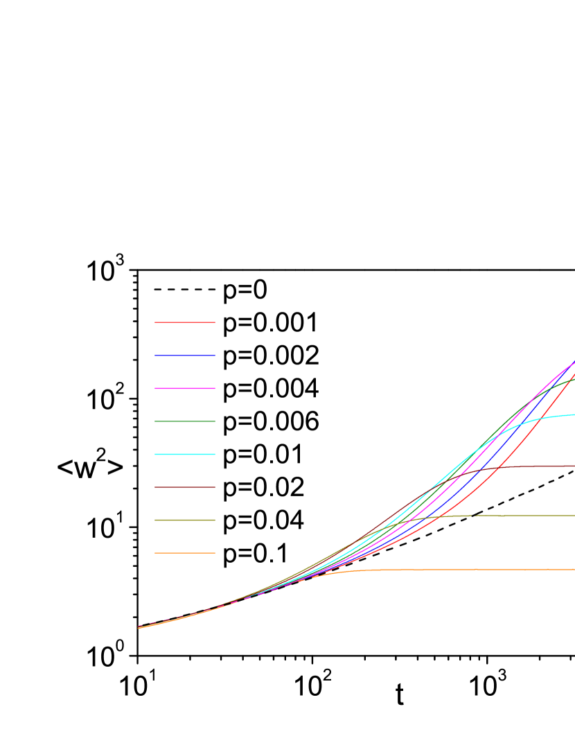
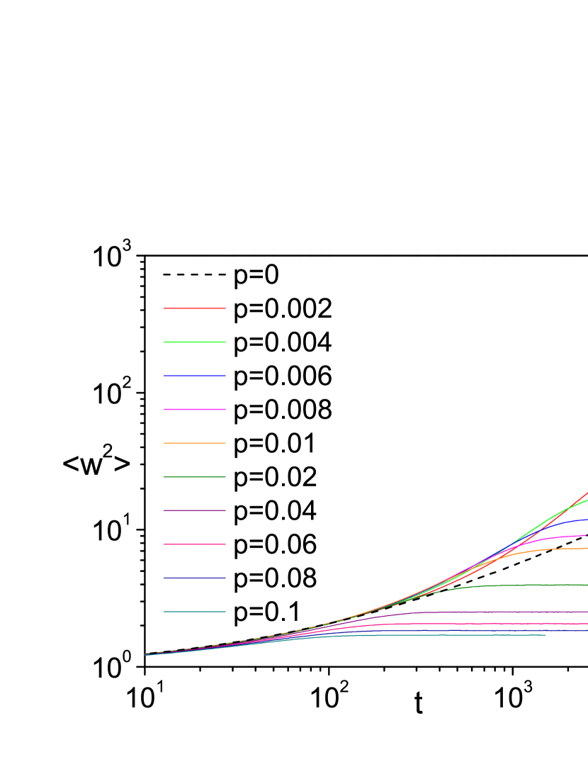
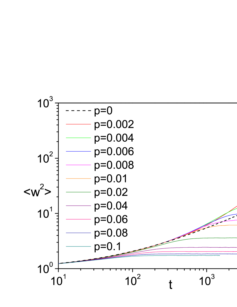
Figure 10 shows the time dependence of the average width for three SW network realizations with PEs. It can be seen that the profile width grows exponentially with time,
| (23) |
and saturates after a time . The larger the value of is, the slower the width grows, and the lower the saturation value is. The width saturates much earlier in the presence of long-range links than in the case . The width saturates after a sufficiently large time on a regular lattice of size korniss2000massively and after a time on SW networks, even for a very small concentration .
a) A–k1
b) A–k2
c) R–k2
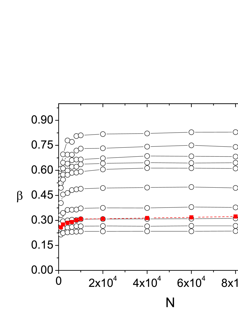
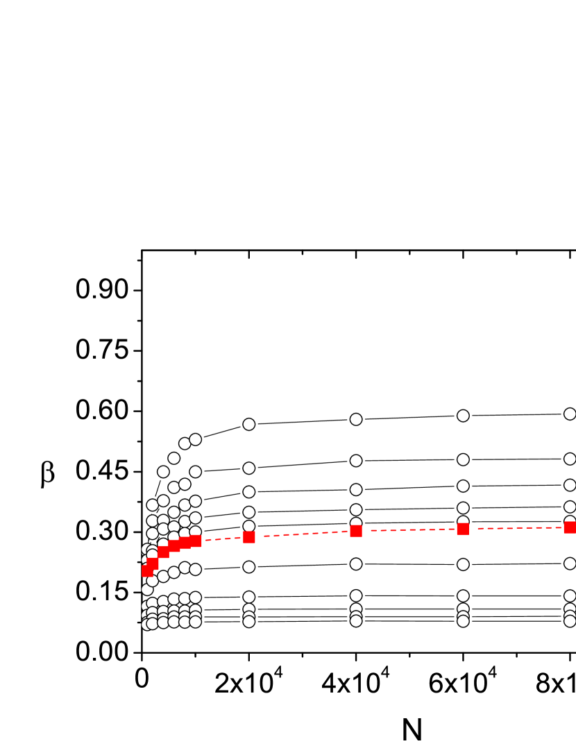
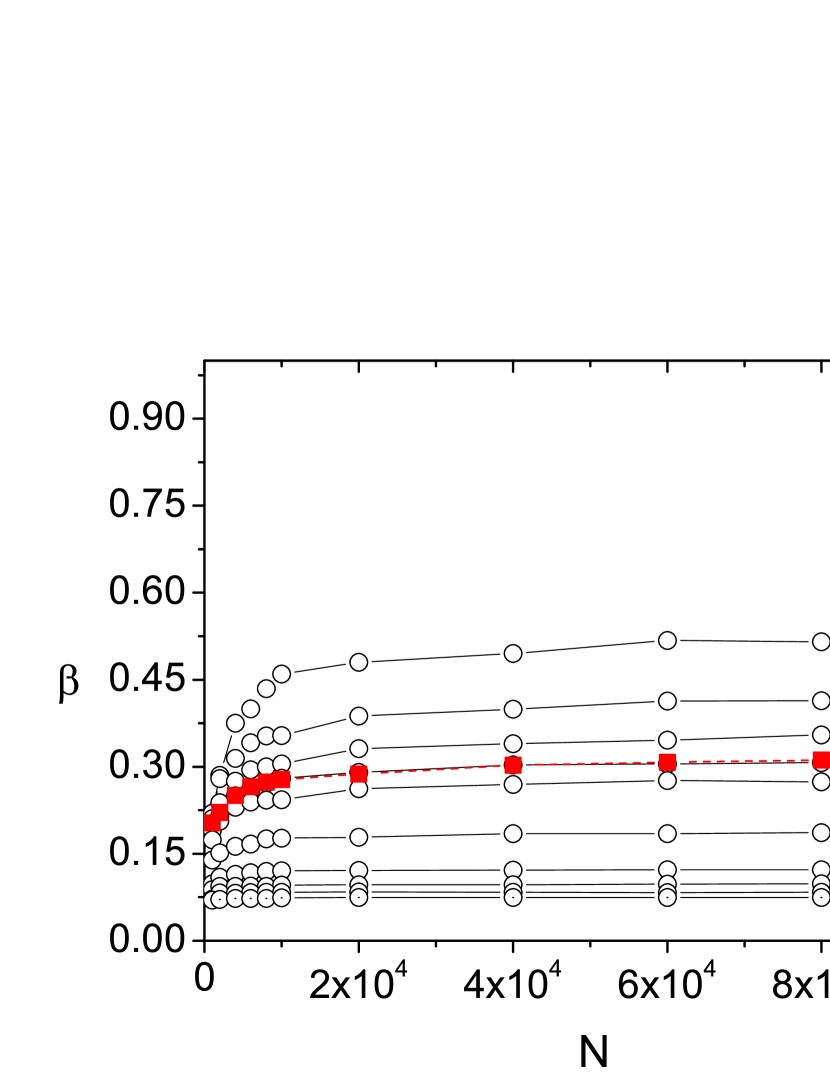
It can also be seen from Fig. 11 that the growth exponent for systems with sufficiently many PEs () becomes constant and independent of . We find the asymptotic values of as using an approximation with power-law corrections. The values of for systems on three SW realizations and various values of the parameter are listed in Table 2. Clearly, the growth exponent decreases as the concentration increases.
a) A–k1
b) A–k2
c) R–k2
Figure 12 shows the exponent as a function of the parameter . We find that for , the exponent depends logarithmically on the concentration :
| (24) |
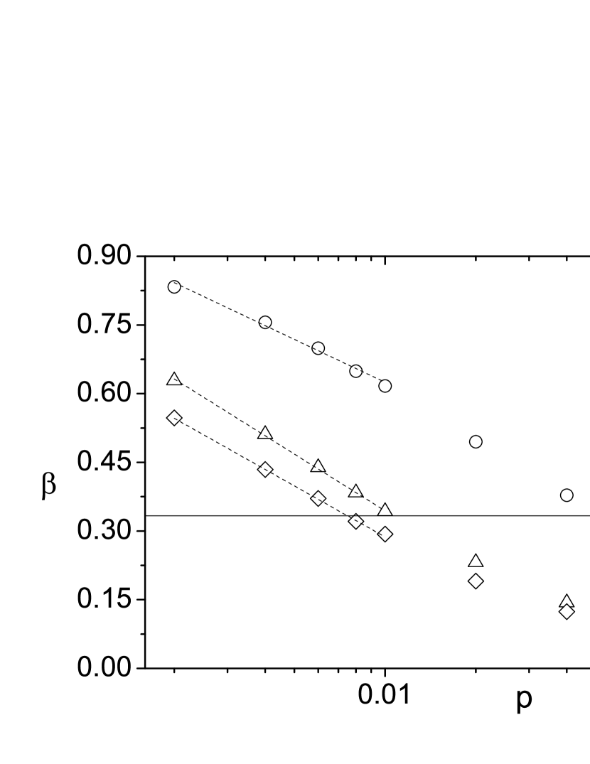
It is important that change of the exponent from SW lattices to regular lattices is singular, as can be seen from Table 2. Even a very small value of changes the exponent dependence from to .
| p | A–k1 | A–k2 | R–k2 |
|---|---|---|---|
| 0 | 0.33280(4) | 0.333(4) | |
| 0.002 | 0.833(3) | 0.629(6) | |
| 0.004 | 0.756(3) | 0.511(5) | |
| 0.006 | 0.699(2) | 0.439(8) | |
| 0.008 | 0.649(2) | 0.38(1) | |
| 0.01 | 0.617(4) | 0.343(4) | |
| 0.02 | 0.4949(8) | 0.232(3) | |
| 0.04 | 0.3783(7) | 0.144(1) | |
| 0.06 | 0.312(1) | 0.1106(8) | |
| 0.08 | 0.2646(8) | 0.093(1) | |
| 0.1 | 0.2341(3) | 0.0791(5) |
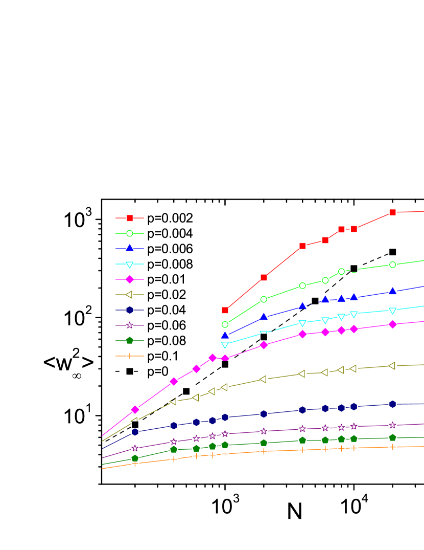
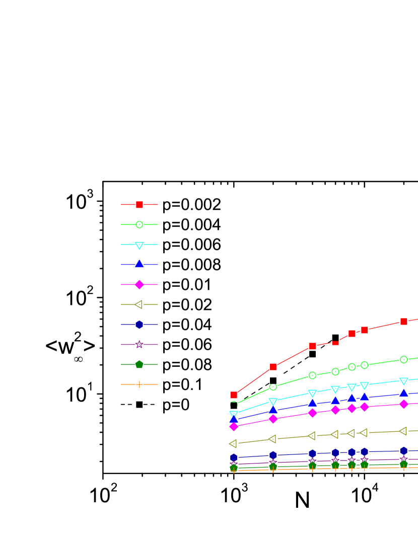
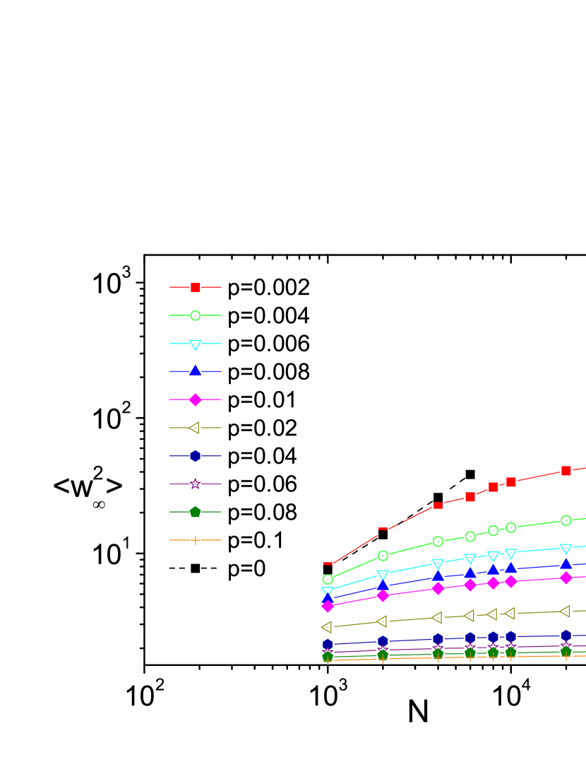
For each set of parameters and , we measure the saturation value of the width by averaging the width over times . Figure 13 shows the steady-state width as a function of the number of PEs for different concentrations . In the case , the steady-state width scales as
| (25) |
where is the roughness exponent approximately equals to (KPZ universality class).
In contrast to expression (25), the average width on SW networks does not increase with the number of PEs, i.e., the roughness exponent . The asymptotic values of in the limit of infinitely many PEs for all three SW network realizations and different values of the parameter are shown in Table III. The average LVT profile width decreases as the parameter increases. Therefore, desynchronization is finite, and its value decreases as increases.
| p | A–k1 | A–k2 | R–k2 |
|---|---|---|---|
| 0 | |||
| 0.002 | 107(5) | 76(3) | |
| 0.004 | 40(3) | 25.1(8) | |
| 0.006 | 20.8(6) | 15.3(7) | |
| 0.008 | 13.3(3) | 11.1(4) | |
| 0.01 | 10.7(7) | 8.3(1) | |
| 0.02 | 4.88(8) | 4.26(6) | |
| 0.04 | 2.81(1) | 2.69(2) | |
| 0.06 | 2.22(1) | 2.201(8) | |
| 0.08 | 1.951(4) | 1.943(6) | |
| 0.1 | 1.783(5) | 1.827(8) |
It can also be seen from Fig. 13 that the saturation value is one order of magnitude less on the SW networks A–k2 and R–k2 than on the network A–k1. The reason is that additional dependencies in the system cause additional synchronization between PEs.
For large , the average LVT profile width on systems with various numbers of PEs has approximately the same small value (Fig. 14). A small average width indicates that PEs are well synchronized, but the utilization (average speed) is low in this case. This indicates that there is some tradeoff between synchronization and utilization, and a compromise can be achieved with a suitable rearrangement of the communication network.
a) A–k1
b) A–k2
c) R–k2
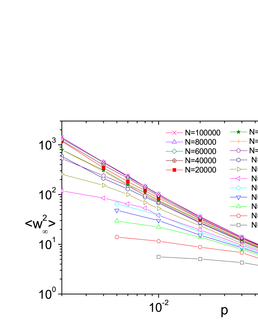
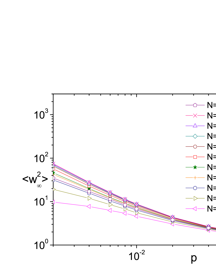
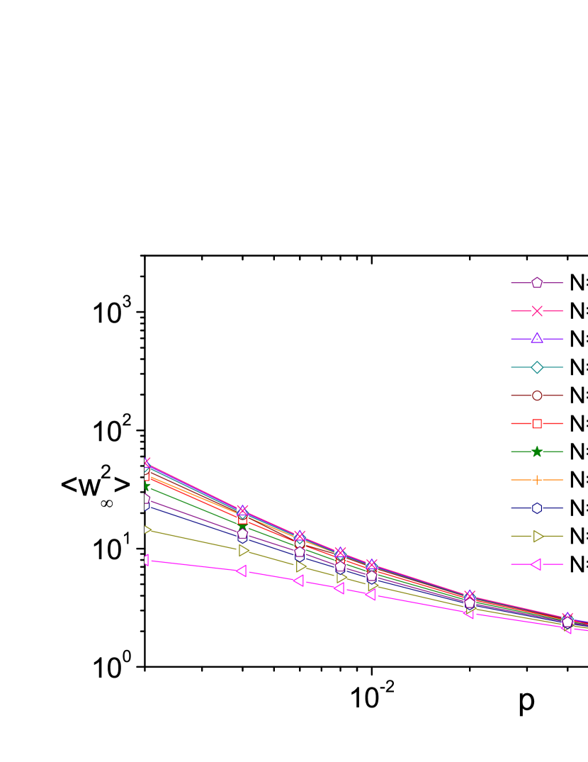
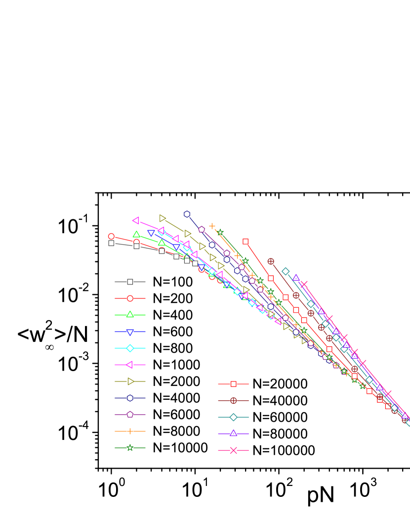
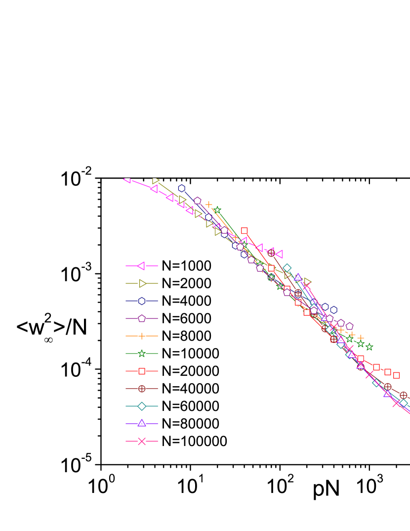
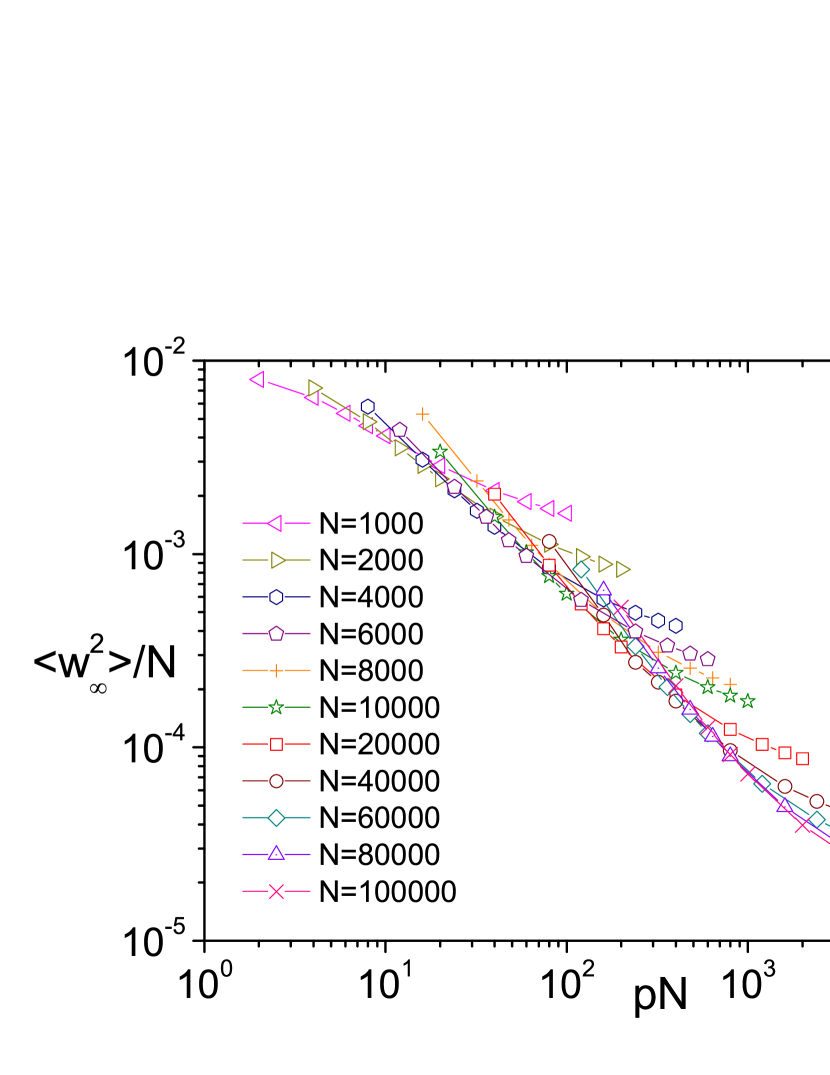
Figure 15 shows the collapse of the curves with a normalized average width as a function of the normalized long-range links . The data collapse is good for the networks A–k2 and R–k2 but rather poor for the network A–k1. This is another argument that clustering affects properties of the LVT evolution model for small .
a) A–k1
b) A–k2
c) R–k2
a) A–k1
b) A–k2
c) R–k2
V Dependence on the local connectivity
Real systems in the natural sciences often have large values of . In this section, we demonstrate how our results are sensitive to the variation of . We present a comparative study of the network properties and PDES behavior for one-dimensional networks with the number of neighbors varying from 2 to 16, i.e., for . In our classification (see Section III), they are respectively called A–k1, A–k2, A–k4, and A–k8.
The variation of the clustering coefficient with the concentration of long-range links is shown in Figure 16. It can be seen that values of the normalized clustering coefficient coincide well for the networks A–k2, A–k4, and A–k8 (we recall that the value of the clustering coefficient for the network A–k1 is zero). For comparison, we plot the variation of the clustering coefficient for the network R–k2 and the corresponding approximation (8).

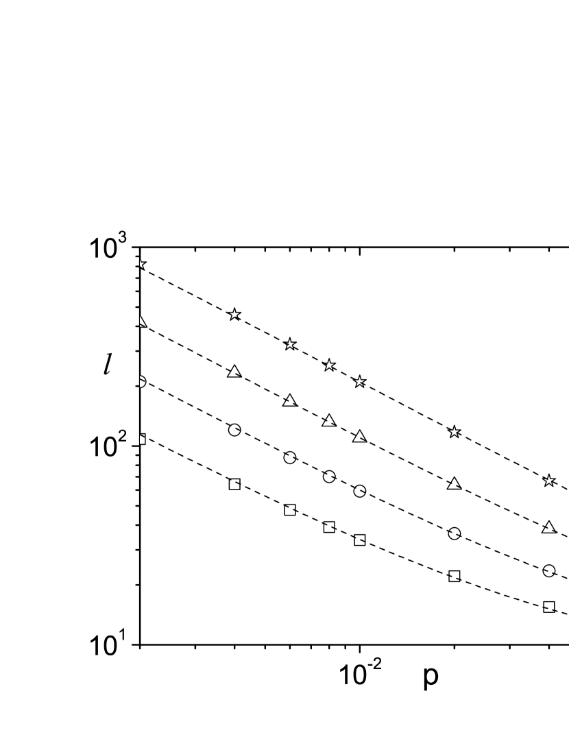
The average shortest path is shown in Figure 17 as a function of the concentration of long-range links and in Figure 18 as a function of the system size. In all cases, the behavior of for the presented range of and is well approximated by Equation (9). It is interesting that the resulting fit in the values of varies slightly around the value and the values of are practically the same, , for all investigated networks except A-k1, for which is much smaller, .

Simulation of the PDES on the SW networks with different leads to some interesting observations. First, we found that the average speed of the time profile can be collapsed on one curve as a function of the concentration . Figures 19 clearly show a good data collapse for for the networks A–k2, A–k4, and A–k8 and rather poor collapse for the network A–k1. Hence, a zero value of the clustering coefficient selects the network A–k1 as a special case, while networks with a nonzero value of demonstrate a universal behavior. Values of , i.e., the average speed on the time profile for the network with , are presented in Table 4. Another interesting observation is that scales with as . The data collapse shown in Figure 19 can therefore be treated in the rescaled variables and .
The data collapse is even more nicely visible for the function normalized by dividing by (or, equivalently, multiplied by ) as shown in Figure 20. Therefore, the exponent given by expressions (21) and (22), which characterize the behavior of for small values of is indeed seems universal for , and 8 with .

| Network type | |
|---|---|
| A–k1 | 0.246410(7) |
| A–k2 | 0.14674(7) |
| A–k4 | 0.08127(4) |
| A–k8 | 0.04299(3) |
The behavior of the average width on regular () lattices A–k1, A–k2, A–k4, and A–k8 demonstrates the same behavior with the growth exponent of KPZ universality class as shown in Figure 21. The larger the value of is, the longer the time required for entering the scaling regime.
Estimates of the values of as a function of are presented in Table 5. It can be seen that attaining the scaling regime for is shifted to the larger network sizes.
In another words, translating our findings into computer science terms, larger values of work in different directions: they suppress desynchronization (width behavior), which is a positive sign, and suppress utilization of processing time (average speed behavior).

| A–k4 | A–k8 | |||
|---|---|---|---|---|
| p | ||||
| 0 | 0.22(2) | 0.291(1) | 0.118(5) | 0.25(1) |
| 0.002 | 0.218(8) | 0.27(1) | 0.045(2) | 0.06(1) |
| 0.004 | 0.148(4) | 0.18(1) | 0.0315(4) | 0.040(2) |
| 0.006 | 0.113(2) | 0.140(6) | 0.027(2) | 0.031(4) |
| 0.008 | 0.094(2) | 0.114(5) | 0.024(2) | 0.027(1) |
| 0.01 | 0.083(3) | 0.095(3) | 0.022(2) | 0.023(1) |
| 0.02 | 0.055(2) | 0.059(4) | 0.0158(3) | 0.165(1) |
| 0.04 | 0.038(2) | 0.039(2) | 0.0113(3) | 0.0116(4) |
| 0.06 | 0.032(1) | 0.0313(5) | 0.0104(5) | 0.0098(5) |
| 0.08 | 0.0261(2) | 0.0272(3) | 0.0078(7) | 0.0086(4) |
| 0.1 | 0.0240(2) | 0.0239(3) | 0.0069(4) | 0.0074(1) |
VI Conclusion
We have investigated the influence of the SW communication topology on the synchronization properties in the conservative PDES algorithm using a model of the evolution of the LVT profile. We simulated the model on several SW network realizations, which differed in their local properties and the procedure for inserting the long-range links. The time evolution of the model on a regular network (with only short-range interaction between PEs) belongs to the KPZ universality class with the critical exponent values and . In contrast, even a small number of long-range links changes the behavior drastically. The growth exponent depends logarithmically on the concentration of long-range links, , and the roughness exponent drops to zero. The average profile speed decreases as a power of the concentration , with for the network A–k1. It seems take universal value for the networks A–k2, A–k4, and A–k8, and it is for the network R–k2. We found a data collapse of the profile width as a function of the concentration for the two realizations of the topology with a nonzero clustering coefficient. The absence of data collapse for the network A–k1 can probably be attributed to the zero clustering coefficient. In other words, the network A–k1 is not quite a conventional SW network: it lacks clustering.
A model of time evolution for the conservative PDES was investigated in guclu2006synchronization ; guclu2004small for an underlying network of the mean-field type where any site is connected by a single link to a randomly chosen site and each site hence has exactly three links and each non-neighbor link is activated with probability . The results in guclu2006synchronization ; guclu2004small seem similar to some of our results (we use the conventional SW network topology) but not all results coincide. The common feature of the two approaches is that the average shortest path grows logarithmically with the number of PEs. For small , it was found in guclu2006synchronization that the average speed of the profile growth is
| (26) |
In contrast, the average speed in our simulations decreases for any values of with a power-law dependence on , . The value of the exponent is universal for the networks with a nonzero clustering coefficient and takes a different value for the network with a zero clustering coefficient.
The same qualitative behavior for the average profile speed and average profile width was reported in guclu2006synchronization ; guclu2004small , but the dependence of the exponents and on and of the average speed on the concentration of long-range links were not analyzed.
We found that value of the clustering coefficient influences the progress of the profile, and we argue that the larger the average coordination number, the slower the profile speed.
In the language of computation processes, the results are as follows. First, additional random long-range communication links in the communication topology of PEs links cause more dependency checks during simulations and reduce the average utilization of PEs, but the utilization remains positive, i.e., the conservative PDES algorithm on SW networks remains free from deadlock. Second, desynchronization becomes finite and decreases with the amount of long-range communications. This enhances data collection and state savings in PDES. The conservative synchronization algorithm of PDES hence becomes fully scalable: (1) the progress rate of simulations remains positive, and (2) desyncronization of the LVT profile becomes finite in the limit of a large number of PEs.
We compared the results on different SW network realizations. All have a short average path, but they differ in the clustering property and the construction method. One SW network has a zero clustering coefficient, and the others are highly clustered. The highly clustered networks differ in their construction (random long-range links were either added or rewired). Qualitatively, the same results were obtained in all cases, i.e., the communication network can be rearranged in any of the presented ways to obtain a well-synchronized PDES algorithm. We found that the model properties depend mainly on the number of long-range communication links and weakly on the way the SW network is constructed. But there is no universal behavior for all cases. For example, the average utilization decreases faster with in the case of SW network with a zero clustering coefficient compared with the SW networks with a high clustering coefficient.
A detailed analysis of the synchronization model of the conservative PDES algorithm on the SW networks allows associating the parameters of the considered model with the example of simulations of the particular models. These in turn can shed light on how to optimize the simulations.
References
- (1) G. R. Joubert, H. Leather, and M. Parsons, Parallel Computing: On the Road to Exascale, Vol. 27 (IOS Press, 2016).
- (2) F. Zhu, Y. Yao, W. Tang, and D. Chen, Future Gener. Comput. Syst. 51, 132 (2015).
- (3) R. M. Fujimoto, Commun. ACM 33, 30 (1990).
- (4) R. M. Fujimoto, ACM Trans. Model. Comput. Simul. (TOMACS) 26, 22 (2016).
- (5) D. C. Richardson, K. J. Walsh, N. Murdoch, and P. Michel, Icarus 212, 427 (2011).
- (6) J. P. Nilmeier and J. Marian, Comput. Phys. Commun. 185, 2479 (2014).
- (7) C. Garcia Cardona, V. Tikare, and S. J. Plimpton, Int. J. Comput. Mater. Sci. Surf. Eng. 4, 37 (2010).
- (8) T. Oppelstrup, D. R. Jefferson, V. V. Bulatov, and L. A. Zepeda-Ruiz, in Proceedings of the 2016 ACM SIGSIM Conference on Principles of Advanced Discrete Simulation (ACM, 2016) pp. 127-130.
- (9) G. Korniss, Z. Toroczkai, M.A. Novotny, and P. A. Rikvold, Phys. Rev. Lett. 84, 1351 (2000).
- (10) M. Kardar, G. Parisi, and Y.-C. Zhang, Phys. Rev. Lett. 56, 889 (1986).
- (11) D. J. Watts and S. H. Strogatz, Nature 393, 440 (1998).
- (12) M. Newman, Networks: an introduction (Oxford University Press, 2010).
- (13) G. Korniss, M. Novotny, H. Guclu, Z. Toroczkai, and P. A. Rikvold, Science 299, 677 (2003).
- (14) H. Guclu, G. Korniss, M.A. Novotny, Z. Toroczkai, and Z. Rácz, Phys. Rev. E 73, 066115 (2006).
- (15) The analogy with surface growth is not perfect in the case of SW topology, because we do not know any physical realizations of such long-range interactions.
- (16) D. J. Watts, Small worlds: the dynamics of networks between order and randomness (Princeton University Press, 1999).
- (17) D. R. Jefferson, ACM Trans. Program. Lang. Syst. (TOPLAS) 7, 404 (1985).
- (18) L. N. Shchur and M.A. Novotny, Phys. Rev. E 70, 026703 (2004).
- (19) Z. Toroczkai, G. Korniss, M. A. Novotny, and H. Guclu, in Computational Complexity and Statistical Physics, edited by A. Percus, G. Istrate, and C. Moore (Oxford University Press, 2006), arXiv/0304617.
- (20) M. D. Humphries and K. Gurney, PloS One 3, e0002051 (2008).
- (21) V. J. Barranca, D. Zhou, and D. Cai, Phys. Rev. E 92, 062822 (2015).
- (22) M. Borassi, A. Chessa, and G. Caldarelli, Phys. Rev. E 92, 032812 (2015).
- (23) A. Barrat and M. Weigt, Eur. Phys. J. B 13, 547 (2000).
- (24) M. E. J. Newman, C. Moore, and D. J. Watts, Phys. Rev. Lett. 84, 3201 (2000).
- (25) M. E. Newman and D. J. Watts, Phys. Lett. A 263, 341 (1999).
- (26) M. E. Newman, Comput. Phys. Commun. 147, 40 (2002).
- (27) D. J. Watts, Am. J. Sociol. 105, 493 (1999).
- (28) J. Krug and P. Meakin, J. Phys. A: Math. Gen. 23, L987 (1990).
- (29) H. Guclu, G. Korniss, Z. Toroczkai, and M. A. Novotny, in Complex Networks (Springer, 2004) pp. 255-275.