Polarized Radiative Transfer in Planetary Atmospheres and the Polarization of Exoplanets

Abstract

We describe the incorporation of polarized radiative transfer into the atmospheric radiative transfer modelling code vstar (Versatile Software for Transfer of Atmospheric Radiation). Using a vector discrete-ordinate radiative transfer code we are able to generate maps of radiance and polarization across the disc of a planet, and integrate over these to get the full-disc polarization. In this way we are able to obtain disc-resolved, phase-resolved and spectrally-resolved intensity and polarization for any of the wide range of atmopsheres that can be modelled with vstar. We have tested the code by reproducing a standard benchmark problem, as well as by comparing with classic calculations of the polarization phase curves of Venus. We apply the code to modelling the polarization phase curves of the hot Jupiter system HD 189733b. We find that the highest polarization amplitudes are produced with optically thick Rayleigh scattering clouds and these would result in a polarization amplitude of 27 ppm for the planetary signal seen in the combined light of the star and planet. A more realistic cloud model consistent with the observed transmission spectrum results is an amplitude of $\sim$20 ppm. Decreasing the optical depth of the cloud, or making the cloud particles more absorbing, both have the effect of increasing the polarization of the reflected light but reducing the amount of reflected light and hence the observed polarization amplitude.

1 Introduction

Polarization is generally ignored in calculations of radiative transfer in studies of the atmospheres of stars and planets. However, all scattering processes polarize light, so a full treatment of radiative transfer should take account of polarization. In particular we expect the reflected light from a planet to be highly polarized when viewed at appropriate angles. This polarization has been a useful tool in studying the atmospheres of solar system objects such as Venus (e.g. Lyot, 1929; Hansen & Hovenier, 1974) and Titan (Tomasko & Smith, 1982; West & Smith, 1991) and there is interest in the potential of using polarization to characterize exoplanet atmospheres. This could be done by observing the small planetary polarization present in the combined light of the star and planet for an unresolved hot Jupiter system (Seager, Whitney & Sasselov, 2000). The effects are small but within the range of the new generation of high precision polarimeters (Hough et al., 2006; Wiktorowicz & Matthews, 2008; Bailey et al., 2015) that can measure polarization at parts per million levels. Polarization measurements could also potentially be used with future space instruments to detect the presence of liquid water in the atmosphere (Bailey, 2007) or on the surface (Zugger et al., 2010) of Earth-like exoplanets.

There have been a number of calculations of polarization for exoplanets (e.g. Seager, Whitney & Sasselov, 2000; Stam et al., 2006; Buenzli & Schmid, 2009; Lucas et al., 2009; Madhusudham & Burrows, 2012; Karalidi & Stam, 2012; Karalidi, Stam & Guirado, 2013). Most of these required specialist codes for handling the polarization case, that are different from those widely used to interpret other exoplanet observations. In this paper we describe the incorporation of polarized radiative transfer into the highly versatile and thouroughly tested vstar (Versatile Software for Transfer of Atmospheric Radiation Bailey & Kedziora-Chudczer, 2012) radiative transfer code. With this code we are able to use a single model to predict the emission spectrum and transmission spectrum as well as the reflected light and polarization phase curves.

vstar has been applied to the atmospheres of the Earth (Bailey et al., 2007a; Cotton, Bailey, & Kedziora-Chudczer, 2014), Venus (Bailey et al., 2008; Bailey, 2009; Cotton et al., 2012; Chamberlain et al., 2013), Jupiter (Kedziora-Chudczer & Bailey, 2011), Titan (Bailey et al., 2011), brown dwarfs (Yurchenko et al., 2014) and extrasolar planets (Zhou et al., 2013, 2015; Mancini et al., 2016). It uses a line-by-line approach to molecular absorption combined with a full treatment of scattering by molecules, clouds and aerosols. Its rigorous approach to radiative transfer has been tested by comparison with standard benchmark problems, and it’s results have been verified by comparison with both Earth atmosphere and stellar atmosphere reference codes (Bailey & Kedziora-Chudczer, 2012).

In section 2 we describe the requirements for polarized radiative transfer, and how we have incorporated this into vstar, making use of a comprehensive vector radiative transfer solver (Spurr, 2006). In section 3 we describe a test of the resulting code against a standard benchmark problem (Garcia & Siewert, 1989) in polarized radiative transfer. In section 4 we describe how to generate polarization images across a planetary disc and to obtain the disc-integrated polarization at any phase angle. As a test of the code we compare our model for the polarization phase curves of Venus with the results of Hansen & Hovenier (1974) in section 5. In section 6 we apply the same methods to the polarization of the exoplanet HD 189733b, first constructing a model for the planet’s atmosphere that is consistent with transit and eclipse observations from space, that is then used to calculate the expected polarization phase curve.

2 Approach

Our approach is similar to that used in the standard version of vstar described by Bailey & Kedziora-Chudczer (2012). Normally, in the non-polarization case we use the disort package (Stamnes et al., 1988) which performs the radiative transfer solution using the discrete-ordinate method. The radiative transfer equation solved in this case has the form:

$$\mu\frac{dI_{\nu}(\tau,\mu,\phi)}{d\tau}=I_{\nu}(\tau,\mu,\phi)-S_{\nu}(\tau,\mu,\phi)$$ (1)

where $I_{\nu}$ is the monochromatic radiance (sometimes referred to as intensity or specific intensity) at frequency $\nu$, and is a function of optical depth $\tau$, and direction $\mu$, $\phi$, where $\mu$ is the cosine of the zenith angle, and $\phi$ is the azimuthal angle. The source function $S_{\nu}$ is given by:

$$S_{\nu}(\tau,\mu,\phi) =\frac{\varpi(\tau)}{4\pi}\int_{0}^{2\pi}\!\int_{-1}^{1}\!P(\mu,\phi;\mu^{\prime},\phi^{\prime})I_{\nu}(\tau,\mu^{\prime},\phi^{\prime})d\mu^{\prime}d\phi^{\prime}$$

$$\mbox{}+(1-\varpi(\tau))B_{\nu}(T)$$ (2)

$$\mbox{}+\frac{\varpi(\tau)F_{\nu}}{4\pi}P(\mu,\phi;\mu_{0},\phi_{0})\exp{(-\tau/\mu_{0})}$$

where the first term describes scattering of radiation into the beam from other directions according to single scattering albedo $\varpi$ and phase function $P(\mu,\phi;\mu^{\prime},\phi^{\prime})$, the second term allows for thermal emission, with $B_{\nu}(T)$ being the Planck function and the third term corresponds to direct illumination of the atmosphere by an external source with flux $\mu_{0}F_{\nu}$ and direction $\mu_{0},\phi_{0}$ (e.g. the Sun).

In order to solve this equation we need to provide, for each atmospheric layer at each wavelength, the temperature $T$, the vertical optical depth $\Delta\tau$, the single scattering albedo $\varpi$ (i.e. what fraction of the optical depth is due to scattering rather than absorption), and the phase function $P(\Theta)$ that describes the angular distribution of scattered light. These quantities are obtained by combining the contributions of line and continuum absorbers and scattering from molecules and particles (clouds and aerosols) as described in detail in Bailey & Kedziora-Chudczer (2012).

2.1 The Vector Radiative Transfer Equation

To take account of polarization we need to replace equations 1 and 2 with the polarized, or vector, radiative transfer equation that has the form:

$$\mu\frac{d\mathbf{I}_{\nu}(\tau,\mu,\phi)}{d\tau}=\mathbf{I}_{\nu}(\tau,\mu,\phi)-\mathbf{S}_{\nu}(\tau,\mu,\phi)$$ (3)

where $\mathbf{I}_{\nu}$ is the Stokes vector with components $\{I,Q,U,V\}$ describing polarized light. The source function is now:

$$\mathbf{S}_{\nu}(\tau,\mu,\phi) =\frac{\varpi(\tau)}{4\pi}\int_{0}^{2\pi}\!\int_{-1}^{1}\!\mathbf{\Pi}(\mu,\phi;\mu^{\prime},\phi^{\prime})\mathbf{I}_{\nu}(\tau,\mu^{\prime},\phi^{\prime})d\mu^{\prime}d\phi^{\prime}$$

$$\mbox{}+(1-\varpi(\tau))B_{\nu}(T)\mathbf{U}$$ (4)

$$\mbox{}+\frac{\varpi(\tau)F_{\nu}}{4\pi}\mathbf{\Pi}(\mu,\phi;\mu_{0},\phi_{0})\exp{(-\tau/\mu_{0})}\mathbf{U}$$

where $\mathbf{U}$ is the unit unpolarized Stokes vector $\{1,0,0,0\}$, and $\mathbf{\Pi}$ is the phase matrix which replaces the phase function used in the scalar case, and describes both the angular distribuiton of scattering and the polarizing effects of scattering. This version of the equation is derived under the assumption that the medium is “macroscopically isotropic and symmetric” (Mishchenko et al., 2002), which is the case if the scattering aerosols are either spherical particles, or randomly-oriented aspherical particles. It would not be valid for particles that had a preferred orientation in the atmosphere. We also assume that the illuminating source is unpolarized.

2.2 The Normalised Scattering Matrix

It can be seen that the additional information we need to provide for the polarization case is the 4 x 4 phase matrix $\mathbf{\Pi}$. In practice we use the normalised scattering matrix $\mathbf{F}$. The two differ in the coordinate system used, with $\mathbf{\Pi}$ being defined in the coordinate system of the atmosphere, while $\mathbf{F}$ is defined relative to the scattering plane (the plane containing the source, scatterer and observer). The phase matrix can be derived from the scattering matrix by applying a coordinate rotation as described in Mishchenko et al. (2002).

Under our assumptions of a macroscopically isotropic and symmetric medium the scattering matrix depends only on the angle $\Theta$ between the incident and scattered light, and has symmetries such that it can be expressed as follows:

$$\mathbf{F}(\Theta)=\begin{bmatrix}a_{1}(\Theta)&b_{1}(\Theta)&0&0\\ b_{1}(\Theta)&a_{2}(\Theta)&0&0\\ 0&0&a_{3}(\Theta)&b_{2}(\Theta)\\ 0&0&-b_{2}(\Theta)&a_{4}(\Theta)\end{bmatrix}$$ (5)

Thus there are six independent elements $(a_{1},a_{2},a_{3},a_{4},b_{1},b_{2})$ in the scattering matrix, and for the special case of spherically symmetric scattering particles, in addition $a_{1}=a_{2}$ and $a_{3}=a_{4}$, so there are only four independent elements.

The scattering matrix is normalised such that:

$$\frac{1}{2}\int_{0}^{\pi}\!a_{1}(\Theta)\sin{\Theta}d\Theta=1$$ (6)

and it can be seen that $a_{1}(\Theta)$ is equivalent to the phase function $P(\Theta)$ used in the scalar radiative transfer equation.

2.3 Expansion in Generalised Spherical Functions

In the scalar case it is common to express the phase function as an expansion in Legendre polynomials

$$P(\Theta)=\sum_{l=0}^{l_{\mbox{\tiny max}}}{\beta_{l}P_{l}(\cos{\Theta})}$$ (7)

where the coefficients $\beta_{l}$ are referred to as the moments of the phase function, and we can choose the value of $l_{\mbox{\tiny max}}$ depending on the accuracy required.

An equivalent approach for the scattering matrix elements required in the polarized case is to expand in generalised spherical functions (de Rooij & van der Stap, 1984; Mishchenko et al., 2002) as follows:

$$a_{1}(\Theta)=\sum_{l=0}^{l_{\mbox{\tiny max}}}{\beta_{l}P_{00}^{l}(\cos{\Theta})}$$ (8)

$$a_{2}(\Theta)+a_{3}(\Theta)=\sum_{l=0}^{l_{\mbox{\tiny max}}}{(\alpha_{l}+\zeta_{l})P_{22}^{l}(\cos{\Theta})}$$ (9)

$$a_{2}(\Theta)-a_{3}(\Theta)=\sum_{l=0}^{l_{\mbox{\tiny max}}}{(\alpha_{l}-\zeta_{l})P_{2,-2}^{l}(\cos{\Theta})}$$ (10)

$$a_{4}(\Theta)=\sum_{l=0}^{l_{\mbox{\tiny max}}}{\delta_{l}P_{00}^{l}(\cos{\Theta})}$$ (11)

$$b_{1}(\Theta)=\sum_{l=0}^{l_{\mbox{\tiny max}}}{\gamma_{l}P_{02}^{l}(\cos{\Theta})}$$ (12)

$$b_{2}(\Theta)=-\sum_{l=0}^{l_{\mbox{\tiny max}}}{\epsilon_{l}P_{02}^{l}(\cos{\Theta})}$$ (13)

The definition and properties of the generalised spherical functions $P_{mn}^{l}$ can be found in appendix B of Mishchenko et al. (2002). The function $P_{00}^{l}$ is identical to the Legendre polynomial $P_{l}$ so equation 8 is the same as equation 7.

The notation shown in equations 8 to 13 using the first six greek letters ($\alpha_{l},\beta_{l},\gamma_{l},\delta_{l},\epsilon_{l},\zeta_{l}$) is a common covention (e.g. Vestrucci & Siewert, 1984; Garcia & Siewert, 1989) and these are sometimes referred to as the Greek constants or Greek coefficients (although in the case of an atmosphere these are not constants, but functions of optical depth and wavelength).

An alternate notation (e.g de Rooij & van der Stap, 1984; Mishchenko et al., 2002) uses ($\alpha_{1}^{l},\alpha_{2}^{l},\alpha_{3}^{l},\alpha_{4}^{l},\beta_{1}^{l},\beta_{2}^{l}$) for the expansion coefficients with

$$\alpha_{1}^{l} =\beta_{l} \alpha_{2}^{l} =\alpha_{l} \alpha_{3}^{l} =\zeta_{l}$$

$$\alpha_{4}^{l} =\delta_{l} \beta_{1}^{l} =\gamma_{l} \beta_{2}^{l} =\epsilon_{l}$$

2.4 Vector Radiative Transfer Solvers

To solve the vector radiative transfer equation as described above we use the Vector Linearised Discrete Ordinate Radiative Transfer (vlidort) code of Spurr (2006) that uses the discrete-ordinate method. We used vlidort version 2.5, the most recent fortran 77 version.

The discrete-ordinate method replaces the integral over $\mu^{\prime}$ that appears in the source function scattering term (equations 2 or 4) by a sum using Gauss’s quadrature formula. This leads to an equation that can be solved using matrix methods. Typically a double Gauss scheme is used in which a separate set of quadrature angles are used for $-1<\mu<0$ and $0<\mu<1$. By increasing the number of quadrature angles (or streams) the accuracy of the angular representation of the radiance field can be improved, at the cost of increased computation time.

The vlidort code is a comprehensive implementation of the discrete-ordinate method for polarized radiative transfer. It has been widely used for applications in Earth atmosphere observation (e.g. Cuesta et al., 2013; Hammer et al., 2016). However, it is equally suitable for applications in astronomy, and Cotton et al. (2017a) used it for modelling stellar atmosphere polarization. In that work stellar atmosphere polarization predictions using vlidort were verified against previous results using different methods from Harrington (2015) and Sonneborn (1982).

We also tried, as an alternative, the rt3 code of Evans & Stephens (1991) that uses the adding-doubling method. This method, is a development of the doubling method, originally introduced by Van de Hulst (e.g. van de Hulst, 1968) and extended to account for polarization by Hansen & Hovenier (1971). We found results from this code to be less accurate in dealing with the benchmark problem described below, and the code was less comprehensive in its capabilities, so we did not continue with it for the later stages of the project.

2.5 Rayleigh Scattering from Molecules

The scattering matrix expansion coefficients for Rayleigh scattering are given in table 1 in terms of the depolarization factor $\rho$ (Spurr, 2006). In the absence of depolarization they become ($\beta_{0}=1.0,\beta_{2}=0.5,\alpha_{2}=3.0,\gamma_{2}=-\sqrt{6}/2$ and $\delta_{1}=1.5$).

The Rayleigh scattering cross section ($\sigma$) is derived from the refractive index of the gas using (Hansen & Travis, 1974):

$$\sigma=\frac{8\pi^{3}(n(\lambda)^{2}-1)^{2}}{3\lambda^{4}N^{2}}\frac{6+3\rho}{6-7\rho}$$ (14)

where $n(\lambda)$ is the wavelength dependent refractive index, $\lambda$ is wavelength and N is the number density (molecules cm^-3) of the gas measured at the same temperature and pressure as the refractive index.

Table 1: Scattering matrix expansion coefficients for Rayleigh scattering

	$\alpha_{l}$	$\beta_{l}$	$\gamma_{l}$	$\delta_{l}$	$\epsilon_{l}$	$\zeta_{l}$
$l=0$	0	1	0	0	0	0
$l=1$	0	0	0	$\frac{3(1-2\rho)}{2+\rho}$	0	0
$l=2$	$\frac{6(1-\rho)}{2+\rho}$	$\frac{1-\rho}{2+\rho}$	$-\frac{\sqrt{6}(1-\rho)}{2+\rho}$	0	0	0

Table 2: Comparison with “L = 13” benchmark test (Garcia & Siewert, 1989)

Stokes	$\mu$	Garcia/Siewert	vstar/vlidort	Difference
I	$-$1.0	0.0549566	0.0549567	+0.0000001
	$-$0.9	0.0904913	0.0904913	+0.0000000
	$-$0.8	0.125601	0.125601	+0.000000
	$-$0.7	0.167810	0.167810	+0.000000
	$-$0.6	0.219343	0.219343	+0.000000
	$-$0.5	0.282944	0.282944	+0.000000
	$-$0.4	0.362682	0.362682	+0.000000
	$-$0.3	0.465232	0.465233	+0.000001
	$-$0.2	0.602877	0.602878	+0.000001
	$-$0.1	0.802239	0.802239	+0.000000
	$-$0.0	1.11633	1.11633	+0.00000
Q	$-$1.0	$-$0.0216088	$-$0.0216889	$-$0.0000001
	$-$0.9	$-$0.0325810	$-$0.0325810	+0.0000000
	$-$0.8	$-$0.0350476	$-$0.0350477	$-$0.0000001
	$-$0.7	$-$0.0349497	$-$0.0349497	+0.0000000
	$-$0.6	$-$0.0327675	$-$0.0327675	+0.0000000
	$-$0.5	$-$0.0286635	$-$0.0286636	$-$0.0000001
	$-$0.4	$-$0.0227539	$-$0.0227539	+0.0000000
	$-$0.3	$-$0.0152402	$-$0.0152402	+0.0000000
	$-$0.2	$-$0.00664174	$-$0.00664175	$-$0.00000001
	$-$0.1	$-$0.00143775	$-$0.00143773	+0.00000002
	$-$0.0	$-$0.00080295	$-$0.00080289	+0.00000006

2.6 Scattering from Particles

The scattering properties of particles (e.g. clouds and aerosols) can be calcuated using Lorenz-Mie theory. vstar uses a Lorenz-Mie scattering code from Mishchenko et al. (2002) that models scattering from a size distribution of spherical particles. This code returns the extinction and scattering cross sections and hence the single scattering albedo. The code also calculates the scattering matrix expansion coefficients needed as input to the radiative transfer solvers.

The number of coefficients needed in equations 8 to 13 to accurately represent the scattering matrix generally increases with the size parameter $x=2\pi a/\lambda$ where $a$ is the particle radius, and $\lambda$ is the wavelength. For $x<$ 1 we are close to the Rayleigh regime and only a small number of expansion coefficients are needed. For large $x$ the number of terms can become much higher. This in turn determines the number of streams needed in the discrete-ordinate radiative transfer solution to accurately represent the angular dependence of the radiation field. The number of streams in each hemisphere should be at least half the number of expansion coefficients for best accuracy.

2.7 Integration into VSTAR

vstar implements a model of an atmosphere with a user-defined number of layers each of which has a specified composition in terms of line and continuum absorbers (atoms, molecules and ions) and potentially a number of aerosol components. The gas phase composition of the layers can be prescribed, or can be obtained from a chemical equilibrium model given specified elemental abundances. vstar combines the optical properties of these various components with appropriate weighting to determine for each layer and at each wavelength the optical properties required for the radiative transfer equation solver (see Bailey & Kedziora-Chudczer, 2012, for a detailed description). The only change required for the polarization case is to replace the scalar radiative transfer solver disort with the vector solver vlidort and calculate the scattering matrix expansion coefficients described above. These are calculated for each layer of the atmosphere at each wavelength being modelled. If a layer of the atmosphere contains more than one scattering component (i.e. different cloud or aerosol types) the optical depths are summed and the expansion coefficents for the components are averaged, weighting according to each components’ contribution to the optical depth.

3 Benchmark Test

The benchmark test we consider is the “L = 13” problem of Garcia & Siewert (1989). In this problem we model scattering of light with wavelength 0.951 $\mu$m from a gamma distribution of spherical particles with effective radius $r_{\mbox{\small eff}}$ = 0.2 $\mu$m, effective variance $v_{\mbox{\small eff}}$ = 0.07 and refractive index 1.44. The single scattering albedo is $\varpi$ = 0.99. The particles are contained in a uniform slab with optical depth $\tau$ = 1, and illuminated by a source at $\mu_{0}$ = 0.2. The slab has a Lambert surface with albedo 0.1 at its base. Garcia & Siewert (1989) tabulate results for this problem accurate to six significant figures. In table 2 we present our results for this problem implemented in vstar. The results presented are for the I and Q Stokes parameters as seen at the top of the atmosphere for values of $\mu$ from 0.0 to -1.0 for the case $\phi-\phi_{0}=0.0$. The vstar calculations used 30 streams in each hemisphere.

For vstar using vlidort the results are in most cases in agreement with the benchmark results to $\pm$1 in the sixth significant figure. Good agreement is also found for other results tabulated by Garcia & Siewert (1989) for this problem using different relative azimuths and optical depths. We note that while vlidort has previously been reported to reproduce this benchmark result, our test, in addition, validates the correct calculation of the scattering matrix expansion from the basic particle properties in vstar.

4 Polarization across a Planetary Disc

4.1 Method

Up to now the models we have considered describe polarization at a single point on a planetary surface that can be represented by a locally plane-parallel atmosphere. However, in many cases we are interested in the distribution of polarization across the visible disc of the planet, or in the integrated polarization from the whole disc. The latter is particularly the case when considering polarization of exoplanets where the planet itself is unresolved.

One approach to integrating over the disc is to use a Gaussian quadrature scheme (Horak, 1950; Hansen & Hovenier, 1974). Stam et al. (2006) describe an efficient way of integrating over the disc of a horizontally homogenous planet. These approaches work well if only the disc-integrated results are needed. However, viewing the distribution of polarization across the disc can be instructive in helping to understand the polarization features seen in the integrated signal. There are also polarization effects such as limb polarization (Schmid, Joos & Tschan, 2006) that, due to symmetry, are lost in the integrated signal. We therefore follow a different approach which allows us to derive from a model an image of the distribution of polarization across the disc, as well as the integrated polarization properties.

We start by considering an orthographic projection of the spherical planet onto a plane in which we define a cartesian coordinate system $x,y$ with coordinates normalised so that the projected radius of the planet is one. An orthographic projection is equivalent to the view of the planet from a large distance. We introduce the coordinates $\zeta$ and $\eta$, that are the longitude and colatitude of a point on the planet related to $x,y$ via:

$$\eta=\arccos{y}$$ (15)

$$\zeta=\arctan{(\frac{x}{\sqrt{1-r^{2}}})}$$ (16)

where $r=\sqrt{(}x^{2}+y^{2})$.

In this coordinate system the “equator” is the plane containing the illuminating star and the observer, and the zero of longitude is at a point immediately below the observer.

We can now obtain the zenith angles $\mu$, $\mu_{0}$ and the relative azimuth $\phi-\phi_{0}$ needed for a radiative transfer solution for any phase angle $\alpha$ using (Horak, 1950):

$$\mu_{0}=\sin{\eta}\cos{(\zeta-\alpha)}$$ (17)

$$\mu=\sin{\eta}\cos{\zeta}$$ (18)

$$\cos{(\phi-\phi_{0})}=\frac{\mu\mu_{0}-\cos{\alpha}}{\sqrt{1-\mu^{2}}\sqrt{1-\mu_{0}^{2}}}$$ (19)

$$\sin{(\phi-\phi_{0})}=\frac{\sin{\alpha}\cos{\eta}}{\sqrt{1-\mu^{2}}\sqrt{1-\mu_{0}^{2}}}$$ (20)

We also need the angle $\kappa$ between the local meridian plane at a point on the planet and the planetary scattering plane (Stam et al., 2006). Polarization vectors derived from a local radiative transfer solution need rotating through this angle to give vectors in our $x,y$ coordinate system.

$$\sin{\kappa}=\frac{\cos{\eta}}{\sqrt{1-\mu^{2}}}$$ (21)

$$\cos{\kappa}=\frac{\sin{\eta}\sin{\zeta}}{\sqrt{1-\mu^{2}}}$$ (22)

Note that the angles $\zeta$, $\phi-\phi_{0}$ and $\kappa$ can range through all four quadrants so must be calcuated in a way that places them in the correct quadrant (e.g. using the atan2 function).

We apply this model by generating a grid of uniformly spaced “pixel centres” across the disc of the planet in the x,y plane. For each point that is within the illuminated disc we use equations 15 to 20 to calculate the corresponding values of $\mu$, $\mu_{0}$, and $\phi-\phi_{0}$. We then perform the vector radiative transfer solution for the atmosphere for this set of geometries with vlidort. Using vlidort it is possible to calculate many values of $\mu$, $\mu_{0}$ and $\phi-\phi_{0}$ in a single computation. This typically allows $\sim$ 100 pixels of a disc image to be computed simultaneously. Time can also be saved because of the symmetry of the situation. Corresponding pixels in the northern and southern hemisphere are equivalent, apart from a change in the sign of $U$, and only need to be computed once.

The resulting Stokes vectors can then be converted to Stokes vectors in the x,y coordinate system by rotating $Q,U$ through $2\kappa$. The resulting data can be plotted as an image of the intensity and polarization vectors of the disc of the planet.

To obtain the disc integrated properties it is simply necessary to integrate the Stokes vector components over the area of the disc as follows using

$$Q_{int}=\int_{-1}^{+1}\!\int_{x1}^{x2}\!Q(x,y)dxdy$$ (23)

for the $Q$ Stokes parameter and similar expressions for $I,U$ and $V$.

The limits on the x integration are (for $\alpha>0$):

$$x_{1}=-\sqrt{(1-y^{2})}\sin{(\alpha+\pi/2)}$$ (24)

$$x_{2}=\sqrt{(1-y^{2})}$$ (25)

To integrate over the grid of equally spaced points we use closed Newton-Cotes formulae of appropriate order for up to four points and extended Newton-Cotes formulae for larger numbers of points (Press et al., 1992) to integrate between the first and last grid points on the illuminated disc. We then add a correction to account for the additional distance from the edges of the disc to the first grid point at each end using the trapezoidal rule.

4.2 Test of Integration Accuracy

To test the accuracy of our integration approach we have run the code on a model that consists of simply a Lambertian reflector with surface albedo of one. A spherical planet with a Lambertian surface has an analytic form (Russell, 1916) for the planetary phase function $\psi(\alpha)$, the variation of reflected flux with phase angle, given by:

$$\psi(\alpha)=\frac{2}{3\pi}a_{s}(\sin{\alpha}+\pi\cos{\alpha}-\alpha\cos{\alpha})$$ (26)

where $a_{s}$ is the surface albedo and $\alpha$ is the phase angle. The results are shown in figure 1 where the integration has been carried out for grids of pixels with 30, 40 or 60 pixels across the equator of the planet. The phase functions obtained by the integration method are almost identical to the analytic version as shown in the upper panel of the plot. The small differences are shown on an expanded scale in the lower panel of the plot. The integrated results generally lie slightly below the analytic results with a little more structure apparent at large phase angles where the number of pixels available becomes smaller at crescent phases. The deviation from the analytic function reaches a little over 1% of the full phase value in the worst case.

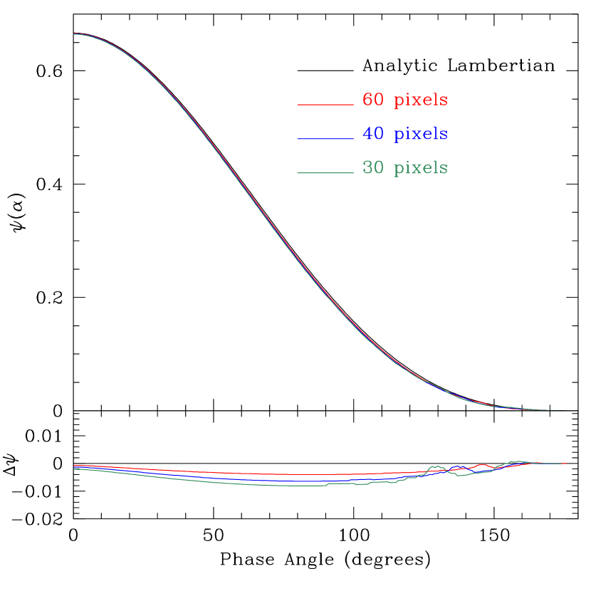
Figure 1: Planetary phase function $\psi(\alpha)$ for a Lambertian reflecting spherical planet from the analytic formula, compared with the results of our integration method. The integration has been carried out over a grid of pixels with either 30, 40 or 60 pixels across the equator of the planet. The bottom panel shows the difference from the analytic formula.

Figure 2: vstar/vlidort models of the polarization phase curve of Venus compared with observations by Lyot (1929) (circles), Coffeen & Gehrels (1969) (crosses) and Dollfus & Coffeen (1970) (plus signs). These models reproduce the modelling of Hansen & Hovenier (1974) almost exactly and can be compared with figures 7 (990 nm), 4 (550 nm) and 9 (365 nm) of that paper. The models are for a single thick cloud layer containing a gamma distribution of spherical particles with effective radius 1.05 $\mu$m and effective variance 0.07 with refractive index and single scattering albedo as given in table 3. The cloud layer also contains Rayleigh scatterers with the Rayleigh scattering optical depth being a fraction $f_{R}=0.045$ of the cloud optical depth at 365 nm.

5 The Polarization of Venus

As a test of integrating polarization across the disc of a planet we have used our code to reproduce the Hansen & Hovenier (1974) (hereafter HH74) study of the polarization phase curves of Venus. Venus is the only planetary atmosphere in the Solar System that can be observed through its full range of phases from the Earth. Hansen & Arking (1971) and HH74 modelled the polarization of Venus and fitted observations over a range of wavelengths. They found that the data could only be fitted if the cloud particles were micron-sized liquid droplets with a refractive index consistent with a 75% concentration of sulfuric acid in water. Together with infrared reflectance measurements these results provided a strong case for sulfuric acid being the main cloud constituent (Sill, 1972; Young, 1973; Pollack et al., 1974). These results have been essentially confirmed by in-situ spacecraft observations.

Table 3: Venus cloud properties used in figure 2

Wavelength (nm)	$n_{r}$	$\varpi$
990	1.43	0.99941
550	1.44	0.99897
365	1.45	0.98427

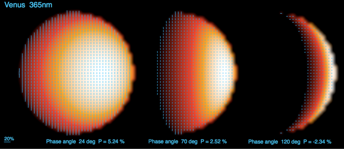
Figure 3: Images of the Venus polarization models for selected phase angles from the same model data as used in the lower panel of figure 2. Polarization vectors are shown overlaid on the intensity distribution. The leftmost image is in the primary rainbow where the polarization is high, the central image is in a region dominated by Rayleigh scattering, and the rightmost image shows a phase where the polarization direction has reversed.

As the main purpose of this test is as a verification of our code, we have reproduced the analysis of HH74 as closely as possible. They used a single layer model to represent the Venus atmosphere. The clouds were modelled as a gamma distribution (Hansen & Travis, 1974; Mishchenko et al., 2002) of spherical particles with effective radius $r_{\mbox{\small eff}}$ = 1.05 $\mu$m, and effective variance $v_{\mbox{\small eff}}$ = 0.07. The real refractive index ($n_{r}$) values are as given in table 3. The imaginary refractive index was zero. However, instead of using the single scattering albedo ($\varpi$) derived from Lorenz-Mie theory (this would be 1 for non-absorbing particles) the values of $\varpi$ in table 3 were used. HH74 derived these values as being those that made the geometric albedo of the planet equal to the observed value. These make the cloud particles significantly absorbing (particularly at 365 nm), and have the effect of increasing the polarization, since light that is not single scattered, is more likely to be absorbed, rather than returned via multiple scattering with little polarization. This is, in effect, incorporating the UV absorber, known to be present in the Venus atmosphere, into the same clouds responsible for the polarization.

The total cloud optical depth was set to $\tau$ = 256 (as used by HH74 and described as equivalent to $\infty$). As well as the clouds the layer includes Rayleigh scatterers with the Rayleigh scattering optical depth set to a fraction $f_{R}$ = 0.045 of the cloud optical depth at 365 nm. In our model we used particles with size much smaller than the wavelength to generate the Rayleigh scattering, although scattering from gas molecules would have the same effect.

Figure 2 shows the resulting polarization phase curves integrated over the illuminated disc compared with observations (mostly full disc polarization measurements) of the polarization of Venus. Positive values refer to polarization perpendicular to the scattering plane, and negative values are parallel to the scattering plane. The model phase curves are essentially identical to those of HH74. They fit the observations reasonably well, and where they deviate a little from observations (e.g. the line is a little below the data for 550 nm at phase angles $\sim$40 – 70) they do so in the same way as the models of HH74. Figure 3 shows images of the polarization vectors overlaid on the intensity image.

It is important to run the calculations with sufficient streams. We used 48 streams in each hemisphere for the 365 nm model, and 32 streams for the 550 and 990 nm. Running the model with too few streams results in a ripple pattern artifact in the resulting phase curve. Figure 4 shows the effect of reducing the number of streams to 16 or 8 for the 550 nm model. In this case the size parameter $x$ is $\sim$12 at 550 nm and $\sim$18 at 365 nm.

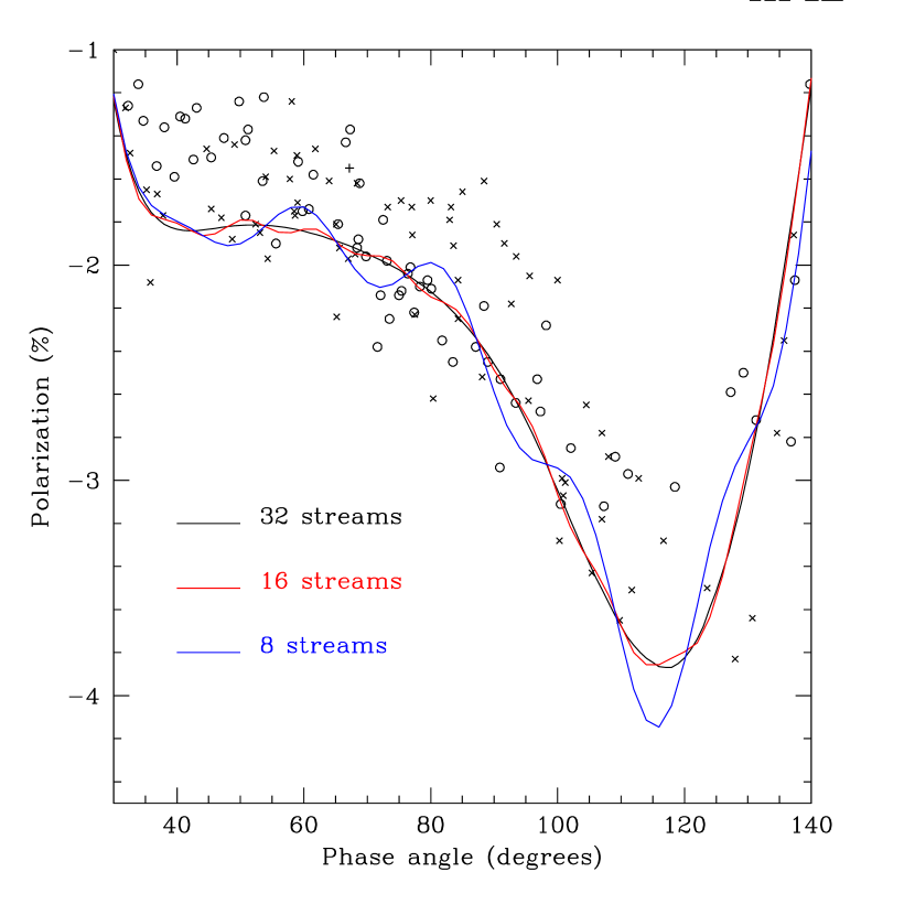
Figure 4: Expanded view of part of the central panel (550 nm) from figure 2 illustrating the “ripple pattern” artifact in the phase curve that occurs when the discrete ordinate radiative transfer is run with too few streams.

The agreement of our results with those of HH74 despite the use of different radiative transfer methods (HH74 used the doubling method) and the agreement of both with the observations provides a good test of our approach.

6 Exoplanet Polarization

Here we consider the polarization of the transiting hot Jupiter HD 189733b. We choose this object because it is one of the best studied exoplanets with a range of data that can be used to constrain an atmospheric model. It also has evidence for the presence of scattering clouds both from transit spectroscopy (Pont et al., 2013), and from a reflected light detection (Evans et al., 2013).

6.1 HD 189733b Model

Before we look at calculating the polarization of the reflected light, we first construct a model of the atmosphere that is consistent with available data from the Hubble Space Telescope (HST) and Spitzer Observatory on the secondary eclipse depths (emission spectrum) and transit depths (transmission spectrum). In our models we assume solar abundances (from Grevesse, Asplund & Sauval, 2007) and equilibrium chemistry. We include absorption from molecules of H₂O, CO, CH₄, CaH, MgH, FeH and CrH, atomic absorption from Na, K, Rb and Cs and collision induced absorption from H₂—H₂ and H₂—He. We also include Rayleigh scattering from H, He and H₂, The methods and data sources are as described in Bailey & Kedziora-Chudczer (2012), except for H₂—H₂ collision induced absorption for which we have used the new HITRAN data (Richard et al., 2012) based on Abel et al. (2011).

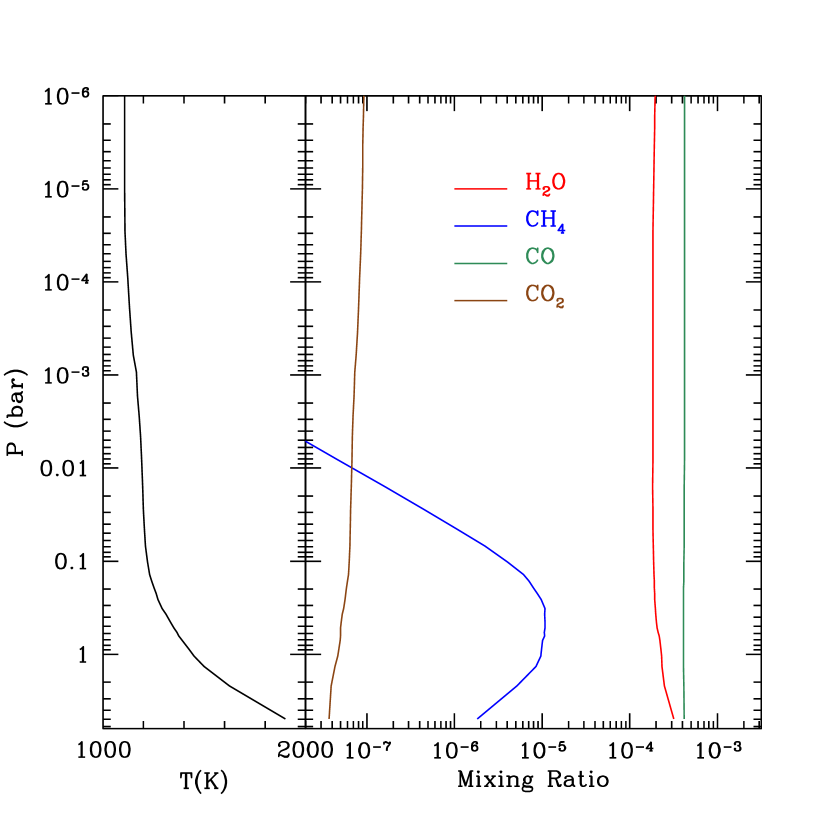
Figure 5: Temperature profile and mixing ratios of important species for our model of HD 189733b

We have adopted a temperature-pressure profile for the atmosphere similar to those found in retrieval studies (e.g. Lee et al., 2012; Line et al., 2014). However, we found we needed somewhat lower temperatures in the 1 bar region than the retrieval models in order to fit the secondary eclipse data in the near-infrared region. The lower temperatures are a consequence of the lower abundances for molecular species that result from our assumptions. Figure 5 shows the adopted temperature profile and the mixing ratios for the species CO, H₂O, CH₄, and CO₂. We note that equilibrium chemistry predicts that CO and H₂O are the most abundant molecular species with relatively low abundances for CO₂ and CH₄. This is in agreement with the results of high-resolution spectroscopy of HD 189733b, which detects CO and H₂O but not CO₂ or CH₄, in both the dayside spectrum (de Kok et al., 2013; Birkby et al., 2013) and the transmission spectrum (Brogi et al., 2016).

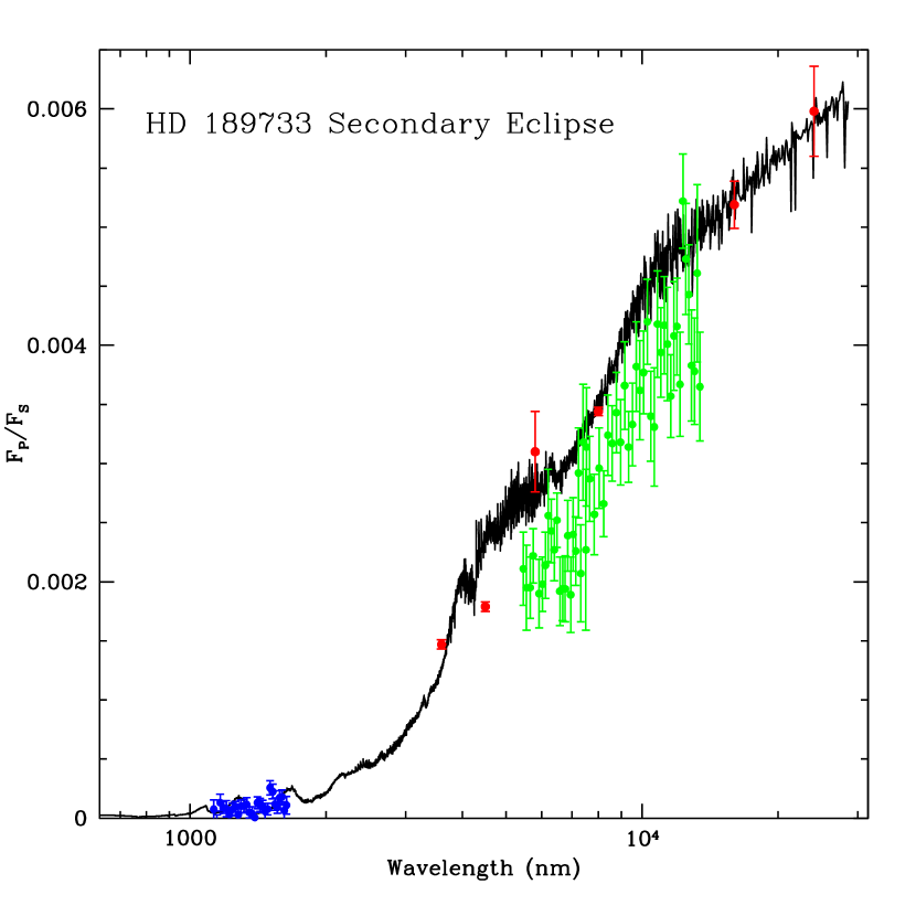
Figure 6: Modelled emission spectrum of HD 189733b (expressed as planet flux divided by stellar flux, F_P/F_S) compared with observations of the HD 189733b secondary eclipse. The observations are, in red, Spitzer photometry from Charbonneau et al. (2008), Agol et al. (2010) and Knutson et al. (2012), in green, Spitzer IRS spectroscopy from Todorov et al. (2014) and, in blue, HST WFC3 spectroscopy from Crouzet et al. (2014). The model also includes the same cloud and haze profile as in figure 7.

In figure 6 we show the emission spectrum predicted by this model compared with observations of the secondary eclipses of HD 189733b. The spectrum is plotted as a fraction of the stellar spectrum, using the Kurucz model for the spectrum of HD 189733 and a value of 0.00033 for $(R_{P}/a)^{2}$ where $R_{P}$ is the planet radius and $a$ is the semi-major axis of the orbit. The model spectrum is a good representation of the WFC3 data (blue points) and the Spitzer photometry (red points). The latest analysis of the Spitzer IRS spectroscopy (Todorov et al., 2014, green points) lies a little below our model, but we prefer to match to the Spitzer photometry that has much smaller errors.

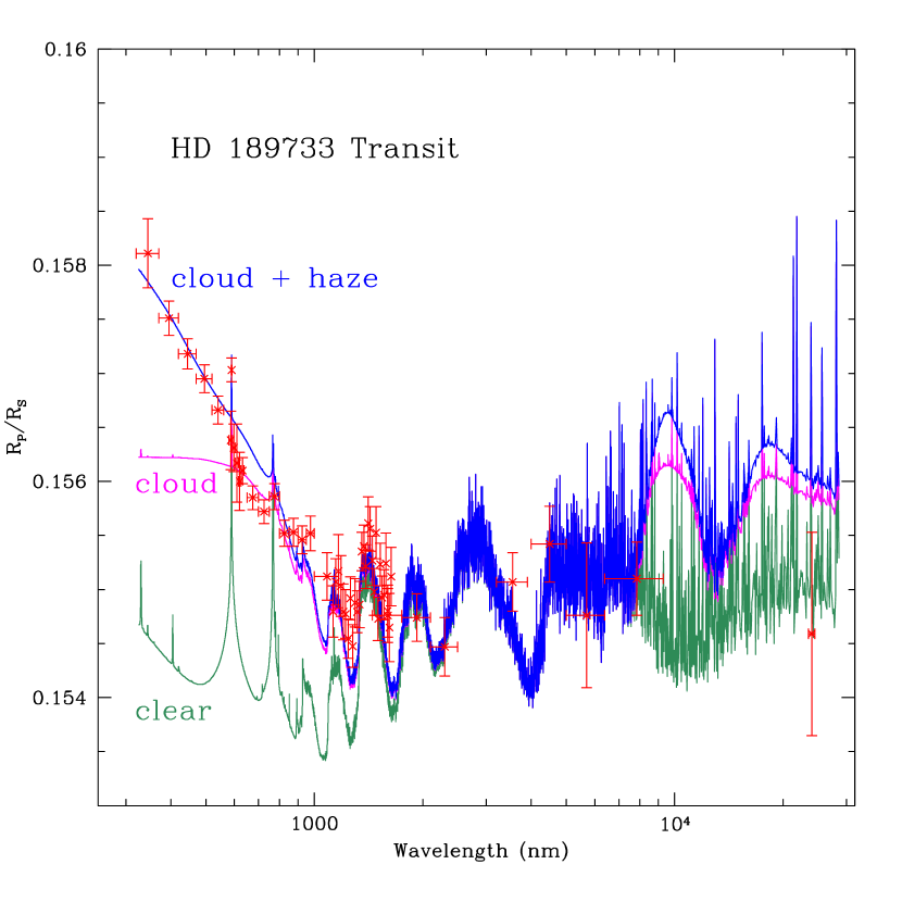
Figure 7: Modelled transmission spectra of HD 189733b (expressed as planet radius divided by stellar radius, R_P/R_S) compared with observations of the HD 189733b transits. The observations, in red, are Spitzer and HST data from Pont et al. (2013) and additional HST WFC3 spectroscopy from McCullough et al. (2014). The models are for a cloud-free (clear) atmosphere, a model with mid-level cloud only, and one with the same cloud plus a high-altitude haze. The cloud and haze here are modelled as 0.05 $\mu$m enstatite particles.

The clouds in the model are adjusted to fit to the observed transit data. We find that the clouds at the required level have very little effect on the emission spectrum which is primarily determined by the temperature profile. Similarly changes to the temperature profile have only a small effect on the transmission spectrum (mostly through the dependence of the scale height on temperature). Thus it requires only a few iterations to derive a model that fits both emission and transmission spectra.

We use transit data from Pont et al. (2013) as well as additional HST/WFC3 data from McCullough et al. (2014). To fit the transmission data we need both a haze component at high altitudes (10^-2 to 10^-4 mbar) as well as a thicker cloud layer at a lower altitude of 0.35 to 3.5 mbar. Figure 7 shows that a clear model does not fit the data at all well over the visible wavelengths. There is a small rise to the blue caused by Rayleigh scattering from molecules, but overall the clear model falls well below the observations from 0.3 to about 1.4 $\mu$m. Adding the cloud layer improves the fit from about 0.7 to 1.4 $\mu$m, but the high altitude haze is needed to also fit the data points in the blue.

We note that McCullough et al. (2014) have proposed an alternate expalanation of the transmission spectrum of HD 189733b, in which unocculted starspots, are responsible for the steep rise at blue wavelengths allowing a clear atmosphere to be consistent with the data. Sing et al. (2016) have looked at the transmission spectra of a larger sample of hot Jupiters and find no correlation between the slope of the transmission feature in the blue, and the stellar activity, thus favouring the cloud interpretation.

We have tried various different compositions for the cloud particles. These include pure Rayleigh particles (i.e. very small, non-absorbing particles) as well as several condensate species that are expected, from chemical models, to be important in hot Jupiter atmospheres. These are the silicates enstatite (MgSiO₃) and forsterite (Mg₂SiO₄) with refractive indices from Scott & Duley (1996), corundum (Al₂O₃, refractive indices from Koike et al., 1995) and iron (Fe, refractive indices from Johnson & Christy, 1974; Ordal et al., 1988). For these species we used a power law size distribution of particles as defined by Hansen & Travis (1974) with effective variance $v_{\mbox{\small eff}}$ = 0.01 and a range of effective radii.

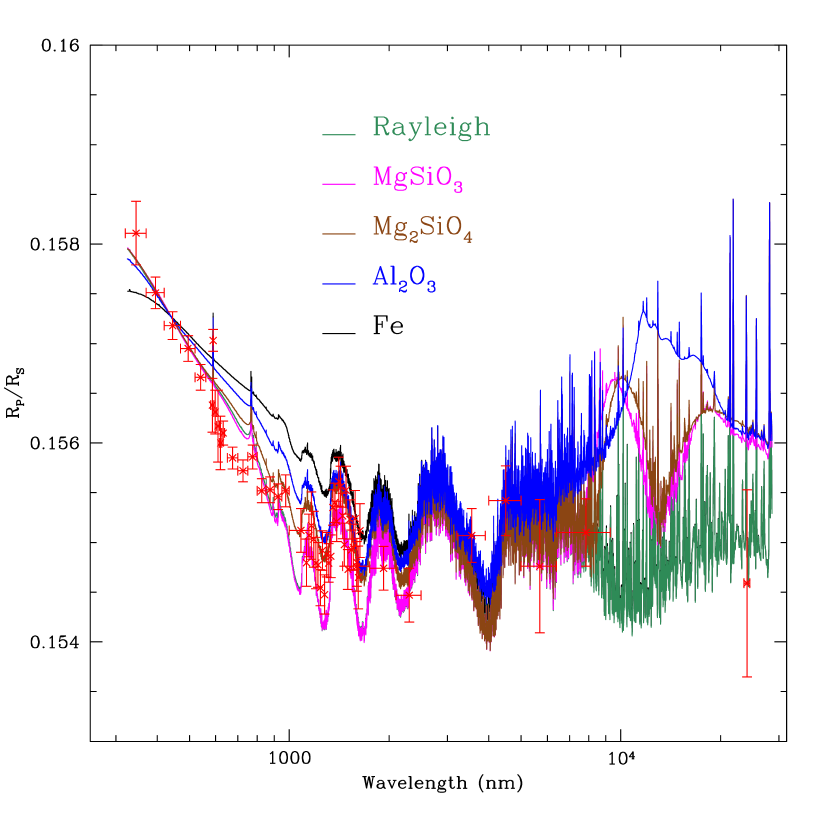
Figure 8: As figure 7, but showing models with different particle compositions, either pure Rayleigh particles (green) or particles with $r_{\mbox{\small eff}}$ = 0.05 $\mu$m composed of enstatite (MgSiO₃), forsterite (Mg₂SiO₄), corundum (Al₂O₃) and iron (Fe). In all cases the same optical depth profile for the cloud at 440 nm as that in figure 7 has been used.

Figure 8 shows a comparison of the predicted transmission spectrum for the different particle compositions. An effective radius of $r_{\mbox{\small eff}}$ = 0.05 $\mu$m has been used in all cases, and the cloud and haze optical depth profile is the same as used in figure 7 and specified at 440 nm wavelength. Note that all the particle types produce a rise in the blue similar to that observed, and with some adjustment of the optical depth profile could probably be made to match the observations better.

It can also be seen from figure 8 that there are substantial differences in the transmission spectrum in the region from 6 to 20 $\mu$m where distinct absorption features are present. This region is not currently well constrained by observations, but future observations with the James Webb Space Telescope (JWST) at these wavelengths could help to determine cloud particle compositions and sizes (Wakeford & Sing, 2015).

The model we have obtained here is not unique, and clearly contains some simplifications. In particular we have assumed that the same model structure applies to the dayside and to the terminator region probed by transmission spectroscopy, when it is known that HD 189733b has temperature structure seen in infrared phase curves (Knutson et al., 2007; Dobbs-Dixon & Agol, 2013). However, the main point here is to show how we can use the same code to model the emission spectrum, transmission spectrum, and reflected light phase curves and polarization phase curves, and to calculate the polarization using a fully realistic model which is consistent with other data.

6.2 Polarization Phase Curves

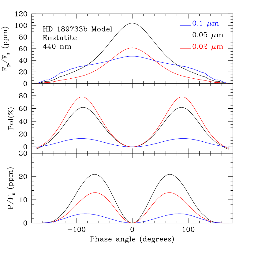
Figure 9: Phase curves and polarization for HD 189733b models with the same cloud/haze optical depth profile as used in figures 7 and 8 for enstatite particles of various sizes. Top panel is the reflected flux from the planet as a fraction of that from the star. Middle panel is the percentage polarization of the integrated reflected light. Lower panel is the polarization fraction in ppm that would be observed in the combined light of the planet and star.

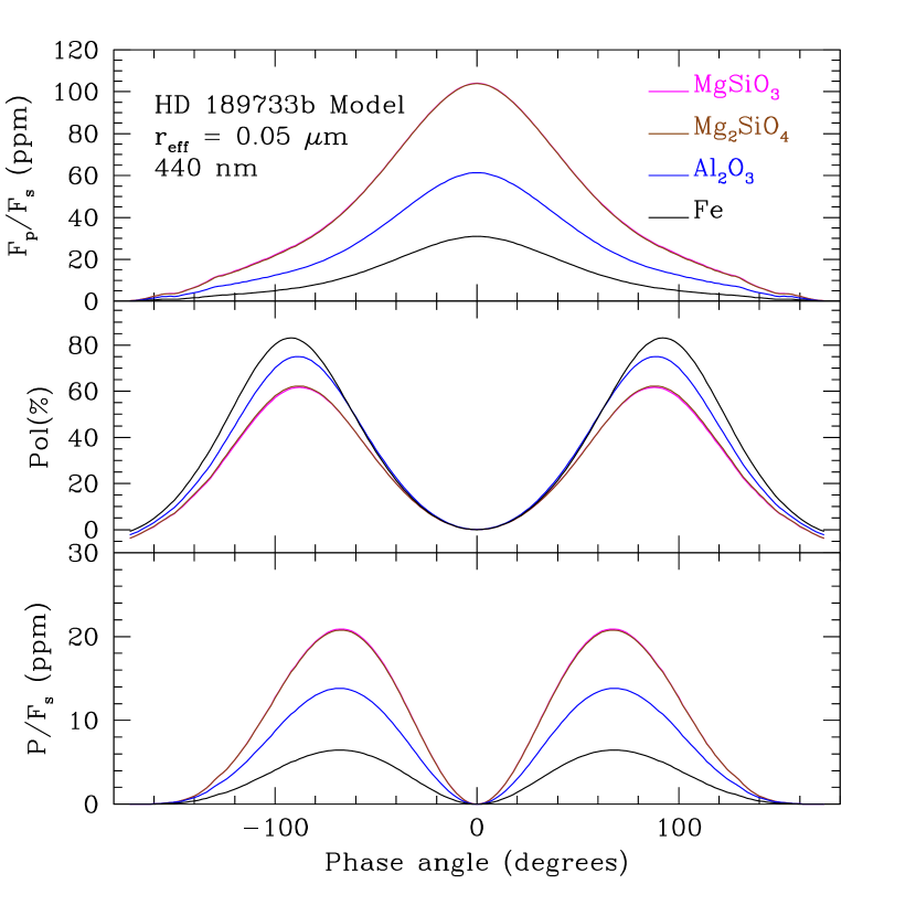
Figure 10: As figure 9 but showing the effect of different haze/cloud particle compositions all with r${}_{\mbox{\small eff}}$ = 0.05 $\mu$m. The curves for the sliciates enstatite and forsterite are almost identical.

We can now calculate the polarization and reflected light phase curves for our model of HD 189733b using the methods outlined in sections 2 and 4. As we are dealing with quite small cloud particles close to the Rayleigh regime, a relatively small number of streams is sufficient. We ran these models with 8 stream in each hemisphere. Figure 9 shows the phase curves for our model using the same cloud/haze optical depth profile as used in figures 7 and 8. The calculations are for 440 nm, a wavelength typically used for observations of the polarization of HD 189733. In this and subsequent plots the top panel shows the reflected light phase curve in parts-per-million (ppm), the middle panel shows the integrated polarization of the planet’s light in per cent, and the bottom panel shows the polarization as a fraction of the light from the star. This is what we would actually observe in a measurement of the polarization of the combined light of the planet and star, if the star is assumed unpolarized. We will refer to this as “observed polarization” in subsequent discussions.

The peak value shown in the top panel, which occurs at zero phase angle, divided by $(R_{P}/a)^{2}$ (0.00033 in our models of HD 189733b) gives the geometric albedo of the planet. For example, a value of 100 ppm (or 0.0001) corresponds to a geometric albedo of 0.303.

Figure 9 shows the effect of particle size for enstatite particles. Particles of 0.05 $\mu$m effective radius produce the highest amplitude for both the phase curve and observed polarization. This is becuase this particle size provides the closest to Rayleigh-like behaviour at this wavelength. Increasing the size to 0.1 $\mu$m moves the particles into the Mie-scattering regime resulting in substantially reduced amplitudes and different phase behaviour. Particles of 0.02 $\mu$m or smaller become increasingly absorbing and this reduces light curve and polarization curve amplitude, although the percentage polarization of the reflected light increases.

Figure 10 shows the effect of particle compositions for 0.05 $\mu$m radius. The silicate particles, enstatite and forsterite, produce almost identical curves. Corundum and Iron particles produce lower amplitudes in reflected light and observed polarization.

Figure 11: Phase curves and polarization for HD 189733b models with a single cloud layer of pure Rayleigh particles with cloud optical depth varied from 0.0 to 10.0. The observed polarization amplitude (lower panel) is highest for the thickest cloud. Decreasing the cloud optical depth increases the fractional polarization of the reflected light, but decreases the albedo of the planet and so decreases the observed polarization.

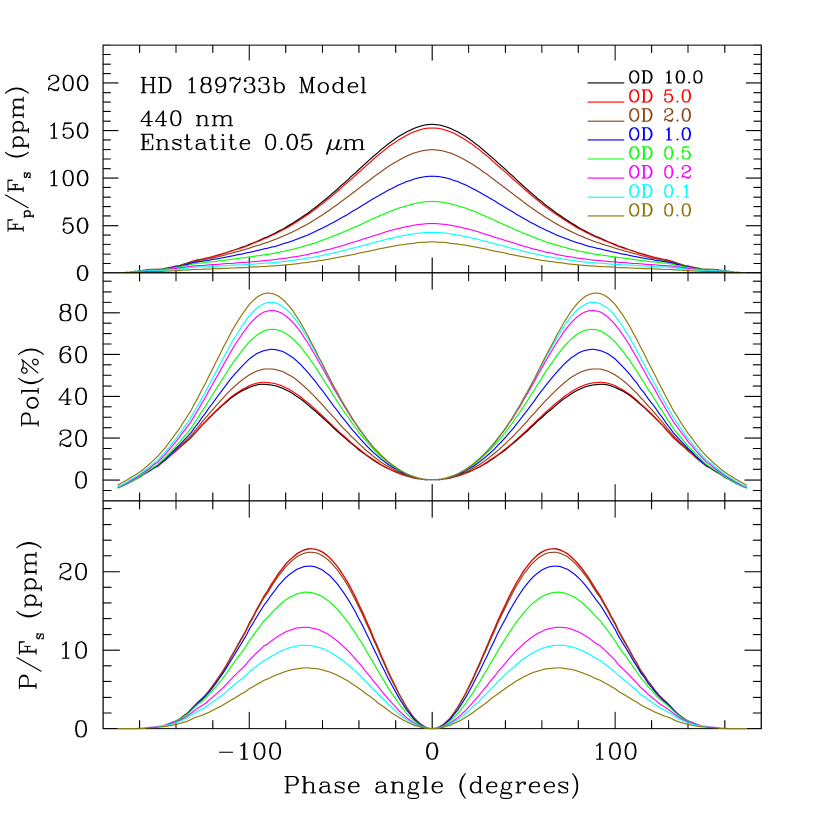
Figure 12: As figure 11 but for clouds composed of 0.05 $\mu$m enstatite particles. The enstatite particles behave similarly to the pure Rayleigh case, but with slightly lower albedo and observed polarization.

In figures 11 and 12 we show the effect of changing the optical depth of the cloud (at 440 nm) from $\tau$ = 0 to 10 for Rayleigh particles and enstatite particles of 0.05 $\mu$m effective radius. In this case we place the cloud in a single layer. It can be seen that the light curve and polarization curve amplitudes are largest for optically thick clouds. As the optical depth of the cloud decreases the percentage polarization of the planetary reflected light increases but the light curve amplitude and consequently observed polarization decreases.

6.3 Polarization Wavelength Dependence

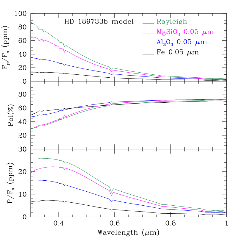
Figure 13: Polarization wavelength dependence for HD 189733b models with the same cloud/haze optical depth profile as used in figures 7 and 8. The results are plotted for phase angle 67 degrees which is approximately where the observed polarization normally peaks. Only the contribution of reflected light is shown here. There will be significant contributions also from thermal emission from the planet at the red end of this plot.

Figure 13 shows the wavelength dependence of the reflected light from the planet and the polarization as seen at a phase angle of 67 degrees, where the observed polarization reaches its peak. The plots are for the cloud optical depth profile used in figures 7 and 8. It can be seen that in general the reflected light fraction and polarization increases to the blue. However, for the enstatite case there is a drop in polarization at the shortest wavelengths as the particles become more absorbing.

6.4 Discussion

The results of the models presented above can be understood as follows. Light that is single scattered from the cloud particles will generally be the most highly polarized. In an optically thick Rayleigh scattering cloud, light that is not single scattered will undergo multiple scattering in the cloud and will eventually be reflected outward after multiple scattering events. This light will tend to have low polarization as the random orientations of the multiple scattering tend to cancel polarization. Models by Buenzli & Schmid (2009) showed that an optically thick Rayleigh scattering atmosphere produces a maximum polarization of 32.6 per cent due to this dilution by multiply-scattered light.

Reducing the optical depth of the cloud increases the chance that light that fails to single scatter upwards will pass through the cloud and be absorbed in lower layers of the atmosphere. This increases the polarization of the reflected light, becuase there is a higher contribution from single scattered light. However, as more light is absorbed, the albedo of the planet and the observed polarization will decrease as a result of this effect.

Making the cloud particles themselves more absorbing, or mixing them with absorbing gases, has the same effect. Light that fails to single scatter is more likely to be absorbed before it can multiple scatter upwards. Once again this increases the polarization of the reflected light but decreases the amount of reflected light and hence the observed polarization.

6.5 Comparison with Previous Modelling of HD 189733b

A key result of our modelling is that the maximum polarization amplitude for HD 189733b is about 27 ppm. An early model by Sengupta (2008) that considered only single scattering gave a polarization amplitude of more than 100 ppm. However, as we show in figure 11 the onset of multiple scattering limits the polarization to much lower values. Lucas et al. (2009) used a Monte-Carlo radiative transfer approach to obtain an upper limit on the polarization of HD 189733b of 26 ppm, in good agreement with our results. Berdyugina et al. (2011) considered a simple model in which the planet reflected as a Lambert sphere with a geometric albedo of 2/3 and was maximally polarized (i.e. 100%) in order to explain the large observed polarization described below. However, as can be seen from figure 11 this combination is not possible. A large geometric albedo can be obtained with optically thick clouds, and a high polarization can be obtained with optically thin clouds, but the two cannot be obtained together.

Kopparla et al. (2016) present a multiple scattering radiative transfer model for HD 189733b, which, like ours, is based on the vlidort code. Their reported polarization amplitudes range from about 40 to 60 ppm, quite different to ours, and above our limit of 27 ppm. However, on examining their results we find that their modelled fluxes for the planet at phase zero are inconsistent with the values expected for the geometric albedo they assume. The flux of the planet as a fraction of that from the star ($f$) is related to the geometric albedo $A_{g}$ by:

$$f=(R_{p}/a)^{2}A_{g}$$ (27)

For HD 189733b $(R_{p}/a)^{2}=0.00033$ so for the geometric albedo of 0.23 which Kopparla et al. (2016) adopt for normalization of their models $f$ should be 76 ppm. In fact the zero phase value shown for their models (e.g. their figure 4) is about 200 ppm. It appears that a scaling error has occurred in the normalization of their model results and all their ppm figures for intensity and polarization are a factor of about 2.6 too high. When their results are corrected for this factor they agree quite well with our results.

6.6 Comparison with Observations

Evans et al. (2013) have reported a reflected light detection of HD 189733b with HST through an observed secondary eclipse depth of 126${}^{+37}_{-36}$ ppm for a wavelength of 290–450 nm. This can be compared with the peak value at zero phase angle in the top panel of figures 9 – 12. It agrees quite well with our value for 0.05 $\mu$m particles and cloud optical depth around 1. Any of our models that matches a 126 ppm reflected light signal, has an observed polarization of $\sim$20 ppm or a little higher. While the wavelength of the HST observation is a little shorter than the 440 nm used for most of our models, we note that figure 13 does not show much change in polarization with wavelength over this range.

A planetary polarization signal from HD 189733b with an amplitude of $\sim$100 ppm has been reported by Berdyugina et al. (2011). However, a signal of this amplitude is not seen in other polarization observations of this object (Wiktorowicz, 2009; Wiktorowicz et al., 2015; Bott et al., 2016). Based on the modelling here we find that such a signal is too large by a factor of four to be explained as due to Rayleigh scattering from the atmosphere of HD 189733b.

Our modelling suggests a more plausible amplitude for the polarization of HD 189733b at 440 nm is $\sim$20 ppm. This is entirely consistent with the observations of Wiktorowicz et al. (2015) and Bott et al. (2016) and with the tentative signal of 29.4 $\pm$ 15.6 ppm reported in the latter work. Further observations are needed to provide a definitive test of the presence of polarized reflected light from this planet.

There are, however, a variety of ways in which the polarization could be lower. If there are no clouds, as in the McCullough et al. (2014) interpretation of the transit data, the polarization drops to only a few ppm (due to Rayleigh scattering from H, He and H₂). The polarization can also be low as a result of the cloud particles being too large (see figure 9) or being more absorbing (figure 10). All these cases would also result in the reflected light intensity being reduced to well below the level reported by Evans et al. (2013). However, the uncertainties on that measurement are such that this cannot be excluded.

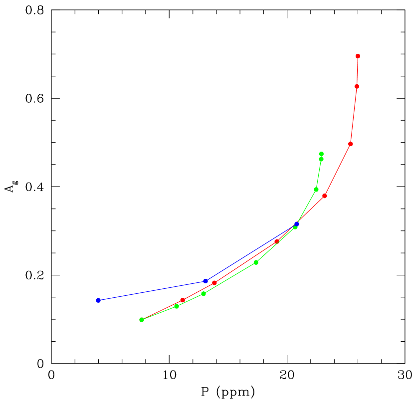
Figure 14: Geometric albedo of planet plotted against polarization amplitude for several of the models of HD 189733b considered previously. Red - models of pure Rayleigh scattering particles as in figure 11. Green - models for 0.05 $\mu$m enstatite particles as in figure 12. Blue - models for different sized enstatite particles as in figure 9.

Another complication with any attempt to detect polarization from HD 189733b is that HD 189733 is an active BY Dra type K dwarf. Recent work by Cotton et al. (2017b) shows that active K dwarfs are typically polarized at levels of $\sim$ 30 ppm, while inactive dwarfs have low polarization. The polarization is most likely the result of differential saturation of spectral lines in the presence of magnetic fields. The stellar polarization is likely to be variable and will confuse any attempt to pick out the planetary signal.

Thus more favourable targets for detecting exoplanet polarization might be hot Jupiters orbiting inactive stars that can be expected to have low polarizations (Cotton et al., 2017b). The polarization technique is not limited to transiting planets. The results in figures 9 to 12 can be used as a guide to estimate the polarization of other planets by scaling the top and bottom panels in proportion to $(R_{P}/a)^{2}$, which has value 0.00033 for the HD 189733b models shown.

6.7 Polarization and Geometric Albedo

A number of previous studies have attempted to use limits on the observed polarization of an exoplanet to set limits on the geometric albedo of the planet (Lucas et al., 2009; Wiktorowicz, 2009; Wiktorowicz et al., 2015). In figure 14 we show the relationship between geometric albedo $A_{g}$ and polarization amplitude for a number of the models we have considered in this study. It can be seen that though there is a general trend for high polarization amplitudes to correspond to high geometric albedos the precise relationships are dependent on the assumptions about particle size and composition.

Thus in general it is hard to set definitive limits on geometric albedo based on polarization observations without making assumptions about the particle properties. In particular most such comparisons are only valid for small Rayleigh-like particles. The example of Venus considered earlier, shows how a high geometric albedo can be achieved with realtively low polarization amplitudes, although the Venus cloud properties are very different from those we expect to find in hot Jupiters.

We further note that the specific limit on geometric albedo of HD 189733b of $A_{g}$ < 0.40 reported by Wiktorowicz et al. (2015) is based on the same modelling as that of Kopparla et al. (2016) which contains a scaling error as noted earlier. When this scaling error is corrected no siginifcant upper limit on the geometric albedo can be set based on these observations.

We can reverse the analysis and used the observed geometric albedo obtained by Evans et al. (2013) together with figure 14 to obtain aother estimate of the predicted polarization amplitude of HD 189733b of $\sim$22 ppm, in reasonable agreement with our earlier estimate. As noted above this estimate is based on the assumption of small Rayleigh-like cloud particles.

7 Conclusions

We have described the modifications required to our vstar radiative transfer code to incorporate polarized radiative transfer. The resulting code enables us to predict the disc-resolved, phase-resolved and spectrally-resolved intensity and polarization for any of the wide range of planetary, substellar and cool-star atmospheres that can be modelled with vstar. The polarized radiative transfer equation is solved using the vlidort code of Spurr (2006) that uses the discrete-ordinate method.

We have tested the code by using it to reproduce a standard benchmark problem in polarized radiative transfer Garcia & Siewert (1989) and find agreement with the benchmark results to 5-6 significant figures. We have also reproduced the calcuations of the polarization phase curves of Venus carried out by Hansen & Hovenier (1974) and obtain essentially identical results.

We have used the code to model the polarization of the hot Jupiter HD 189733b. We first construct a model of the atmosphere that is consistent with the observed emission and transmission spectra. We then calculate the polarization phase curves predicted by that model. We are able to use the same code to model the emission, transmission, reflection and polarization properties of the atmosphere. We predict a polarization amplitude of $\sim$20 ppm for a model consistent with other observations including the Evans et al. (2013) detection of reflected light. The maximum polarization amplitude we can obtain is $\sim$27 ppm achieved with optically thick Rayleigh scattering clouds. The predictions are consistent with polarization observations reported by Bott et al. (2016) and Wiktorowicz et al. (2015).

The detection of polarization in HD189733 at about the predicted level would be strong evidence for the presence of clouds and would rule out clear models such as that of McCullough et al. (2014). A clear atmosphere would result in a low polarization amplitude of only a few ppm. Intermediate levels of polarization may indicate that the cloud particles are smaller or more absorbing. In this case the reflected light intensity will drop below the value reported by Evans et al. (2013). The results can be scaled to other hot Jupiter systems. We note that hot Jupiters orbiting inactive stars may be better targets for polarimetric detection than HD 189733b due to the lower polarization of the host star (Cotton et al., 2017b).

References

- Abel et al. (2011) Abel, M., Frommhold, L., Li, X., Hunt, K.L.C., 2011, J. Phys. Chem. A, 115, 6805
- Agol et al. (2010) Agol, E., Cowan, N.B., Knutson, H.A., Deming, D., Steffen, J.H., Henry, G.W., Charbonneau, D., 2010, ApJ, 721, 1861
- Bailey (2007) Bailey, J., 2007, Astrobiology, 7, 320
- Bailey (2009) Bailey, J., 2009, Icarus, 201, 444
- Bailey & Kedziora-Chudczer (2012) Bailey, J., Kedziora-Chudczer, L., 2012, MNRAS, 419, 1913
- Bailey et al. (2007a) Bailey, J., Simpson, A., Crisp, D., 2007, PASP, 119, 228
- Bailey et al. (2008) Bailey, J., Meadows, V.S., Chamberlain, S., Crisp, D., 2008b, Icarus, 197, 247
- Bailey et al. (2011) Bailey, J., Ahlsved, L., Meadows, V.S., 2011, Icarus, 213, 218
- Bailey et al. (2015) Bailey, J., Kedziora-Chudczer, L., Cotton, D.V., Bott, K., Hough, J.H., Lucas, P.W., 2015, MNRAS, 449, 3064
- Berdyugina et al. (2011) Berdyugina, S.V., Berdyugin, A.V., Fluri, D.M., Piirola, V., 2011, ApJL, 728, L6
- Birkby et al. (2013) Birkby, J.L., de Kok, R.J., Brogi, M., de Mooij, E.J.W., Schwarz, H., Albrecht, S., Snellen, I.A.G., 2013, MNRAS, 436, L35
- Brogi et al. (2016) Brogi, M., de Kok, R.J., Albrecht, S., Snellen, I.A.G., Birkby, J.L., Schwarz, H., 2016, ApJ, 817, 106
- Bott et al. (2016) Bott, K., Bailey, J., Kedziora-Chudczer, L., Cotton, D.V., Lucas. P.W., Marshall, J.P., Hough, J.H., 2016, MNRAS, 459, L109
- Buenzli & Schmid (2009) Buenzli, E., Schmid, H.M., 2009, A&A, 504, 259
- Chamberlain et al. (2013) Chamberlain, S., Bailey, J., Crisp, D., Meadows, V.S., 2013, Icarus, 222, 364
- Charbonneau et al. (2008) Charbonneau, D., Knutson, H.A., Barman, T., Allen, L.E., Mayor, M., Megeath, S.T., Queloz, D., Udry, S., 2008, ApJ, 686, 1341.
- Coffeen & Gehrels (1969) Coffeen, D.L., Gehrels, T., 1969, A&A, 74, 433
- Cotton et al. (2012) Cotton, D.V., Bailey, J., Crisp, D., Meadows, V.S., 2012, Icarus, 217, 570
- Cotton, Bailey, & Kedziora-Chudczer (2014) Cotton, D.V., Bailey, J., Kedziora-Chudczer, L., 2014, MNRAS, 439, 387
- Cotton et al. (2017a) Cotton, D.V., Bailey, J., Howarth, I.D., Bott, K., Kedziora-Chudczer, L., Lucas, P.W., Hough, J.H., 2017a, Nature Ast., 1, 690
- Cotton et al. (2017b) Cotton, D.V., Marshall, J.P., Bailey, J., Kedziora-Chudczer, L., Bott, K., Marsden, S.C., Carter, B.D., 2017b, MNRAS, 467, 873
- Crouzet et al. (2014) Crouzet, N., McCullough, P.R., Deming, D., Madhusuhan, N., 2014, ApJ, 795, 166
- Cuesta et al. (2013) Cuesta, J., et al., Atmos. Chem. Phys., 13, 9675
- de Kok et al. (2013) de Kok, R.J., Brogi, M., Snellen, I.A.G., Birkby, J., Albrecht, S., de Mooij, E.W.J., 2013, A&A, 554, A82
- de Rooij & van der Stap (1984) de Rooij, W.A., van der Stap, C.C.A.H., 1984, AJ, 131, 237
- Dobbs-Dixon & Agol (2013) Dobbs-Dixon, I., Agol, E., 2013, MNRAS, 435, 3159
- Dollfus & Coffeen (1970) Dollfus, A., Coffeen, D.L., 1970, A&A, 8, 251
- Evans & Stephens (1991) Evans, K.F. & Stephens, G.L., 1991, J. Quant. Spectrosc. Radiative Transfer, 46, 415.
- Evans et al. (2013) Evans, T.M. et al., 2013, ApJ, 772, L16
- Garcia & Siewert (1989) Garcia, R.D.M., & Siewert, C.E., J. Quant. Spectrosc. Radiative Transfer, 41, 117
- Grevesse, Asplund & Sauval (2007) Grevesse, N., Asplund, M., Sauval, A.J., 2007, SSRv, 130, 15
- Hammer et al. (2016) Hammer, M.S., Martin, R.V., van Donkelaar, A., Buchard, V., Torres, O., Ridley, D.A., Spurr, R.J.D., 2016, Atmos. Chem. Phys., 16, 2507
- Hansen & Hovenier (1971) Hansen, J.E., & Hovenier, J.W., 1971, J. Quant. Spectrosc. Radiative Transfer, 11, 809
- Hansen & Arking (1971) Hansen, J.E., & Arking, A., 1971, Science, 171, 669
- Hansen & Hovenier (1974) Hansen, J.E. & Hovenier, J.W., 1974, J. Atmos. Sci., 31, 1137
- Hansen & Travis (1974) Hansen, J.E. & Travis, L.D., 1974, Space Sci. Rev., 16, 527
- Harrington (2015) Harrington, J.P., 2015, Proc. IAU, 305, 395
- Horak (1950) Horak, H.G., 1950, ApJ, 112, 445
- Hough et al. (2006) Hough, J.H., Lucas, P.W., Bailey, J.A., Tamura, M., Hirst, E., Harrison, D., Bartholomew-Briggs, M., 2006, PASP, 118, 1302
- Johnson & Christy (1974) Johnson, P.B., Christy, R.W., 1974, Phys. Rev. B9, 5056
- Karalidi & Stam (2012) Karalidi, T. & Stam, D.M., 2012, A&A, 546, A56
- Karalidi et al. (2013) Karalidi, T., Stam, D.M., Guirado, D., 2013, A&A, 555, A127
- Kedziora-Chudczer & Bailey (2011) Kedziora-Chudczer, L., and Bailey, J., 2011, MNRAS, 414, 1483
- Knutson et al. (2007) Knutson, H.A. et al., 2007, Nature, 447, 183
- Knutson et al. (2012) Knutson, H.A. et al., 2012, ApJ, 754, 22
- Koike et al. (1995) Koike, C., Kaito, C., Yamamoto, T., Shibai, H., Kimura, S., Suto, ., 1995, Icarus, 114, 203
- Kopparla et al. (2016) Kopparla, P., Natraj, V., Zhang, X., Swain, M.R., Wiktorowicz, S.J., Yung, Y.L., 2016, ApJ, 817, 32
- Lee et al. (2012) Lee, J.-M., Fletcher, L.N., Irwin, P.G.J., 2012, MNRAS, 420, 170
- Line et al. (2014) Line, M.R., Knutson, H., Wolf, A.S., Yung, Y.L., 2014, ApJ, 783, 70
- Lucas et al. (2009) Lucas, P.W., Hough, J.H., Bailey, J.A., Tamura, M., Hirst, E., Harrison, D., 2009, MNRAS, 393, 229
- Lyot (1929) Lyot, B., 1929, Ann. Observ, Paris (Meudon) 8, 1
- Mancini et al. (2016) Mancini, L., Kemmer, J., Southworth, J., Bott, K., Molliere, P., Ciceri, S., Chen, G., Henning, Th., 2016, MNRAS, 459, 1393
- Madhusudham & Burrows (2012) Madhusudham, N. & Burrows, A., ApJ, 747, 25
- McCullough et al. (2014) McCullough, P.R., Crouzet, N., Deming, D., Madhusudhan, N., 2014, ApJ, 791, 55
- Mishchenko et al. (2002) Mishchenko, M.I., Travis, L.D., Lacis, A.A., 2002, Scattering, Absorption and Emission of Light by Small Particles. Cambridge Univ. Press, Cambridge
- Ordal et al. (1988) Ordal, M.A., Bell, R.J., Alexander, R.W., Newquist, L.A., Querry, M.R., 1988, Appl. Opt. 27, 1203
- Pollack et al. (1974) Pollack, J.B. et al., 1974, Icarus, 23, 8
- Pont et al. (2013) Pont, F., Sing, D.K., Gibson, N.P., Aigrain, S., Henry, G., Husnoo, N., 2013, MNRAS, 432, 2917
- Press et al. (1992) Press, W.H., Teukosky, S.A., Vetterling, W.T., Flannery, B.P., 1992, Numerical Recipes, 2nd edition, Cambridge Univ. Press, Cambridge
- Richard et al. (2012) Rchard, C. et al., 2012, J. Quant. Spectrosc. Radiative Transfer, 113, 1276
- Russell (1916) Russell, H.N., 1916, ApJ, 43, 173
- Seager et al. (2000) Seager, S., Whitney, B.A., Sasselov, D., 2000, ApJ, 540, 504
- Schmid, Joos & Tschan (2006) Schmid, H.M., Joos, F., Tschan, D., A&A, 452, 657
- Scott & Duley (1996) Scott, A., Duley, W.W., 1996, ApJS, 105, 401
- Sengupta (2008) Sengupta, S., 2008, ApJ, 683, L195
- Sill (1972) Sill, G.T., 1972, Commun. Lunar Planet Lab., 9, 191
- Sing et al. (2016) Sing, D.K. et al., 2016, Nature, 529, 59
- Sonneborn (1982) Sonneborn, G., 1982, in Jaschek, M & Groth, H.-G. (eds), Be Stars, IAU Symp. 98, Reidel, Dordrecht, pp 493-495
- Stam et al. (2006) Stam, D.M., de Rooij, W.A., Cornet, G., Hovenier, J.W., 2006, A&A, 452, 669
- Spurr (2006) Spurr, R., 2006, J. Quant. Spectrosc. Radiative Transfer, 102, 316.
- Stamnes et al. (1988) Stamnes, K., Tsay, S.C., Wiscombe, W., Jayaweera, K., 1988, Appl. Opt., 27, 2502.
- Tomasko & Smith (1982) Tomasko, M.G., Smith, P.H., 1982, Icarus, 51, 65
- Todorov et al. (2014) Todorov, K.O., Deming, D., Burrows, A., Grillmair, C.J., 2014, ApJ, 796, 100
- van de Hulst (1968) van de Hulst, H.C., 1969, J. Comp. Phys., 3, 291
- West & Smith (1991) West, R.A., Smith, P.H., 1991, Icarus, 90, 330
- Vestrucci & Siewert (1984) Vestrucci, P., & Siewert, C.E., 1984, J. Quant. Spectrosc. Radiative Transfer, 31, 177
- Wakeford & Sing (2015) Wakeford, H.R., Sing, D.K., 2015, A&A, 573, A122
- Wiktorowicz (2009) Wiktorowicz, S.J., 2009, ApJ, 696, 1116
- Wiktorowicz & Matthews (2008) Wiktorowicz, S.J. & Matthews, K., 2008, PASP, 120, 1282
- Wiktorowicz et al. (2015) Wiktorowicz, S.J. et al., 2015, ApJ, 813, 48
- Young (1973) Young, A.T., 1973, Icarus, 18, 564
- Yurchenko et al. (2014) Yurchenko, S.N., Tennyson, J., Bailey, J., Hollis, M.D.J., Tinetti, G., 2014, PNAS, 111, 9379
- Zhou et al. (2013) Zhou, G., Kedziora-Chudczer, L., Bayliss, D.D.R., Bailey, J., 2013, ApJ, 774, 118
- Zhou et al. (2015) Zhou, G., Bayliss, D.D.R., Kedziora-Chudczer, L., Salter, G., Tinney, C.G., Bailey, J., 2015, MNRAS, 445, 2746
- Zugger et al. (2010) Zugger, M.E., Kasting, J.F., Williams, D.M., Kane, T.J., Philbrick, C.R., 2010, ApJ, 723, 1168