Evaluating the Jones polynomial with tensor networks
Abstract
We introduce tensor network contraction algorithms for the evaluation of the Jones polynomial of arbitrary knots. The value of the Jones polynomial of a knot is reduces to the partition function of a -state anisotropic Potts model with complex interactions, which is defined on a planar signed graph that corresponds to the knot. For any integer , we cast this partition function into tensor network form, which inherits the interaction graph structure of the Potts model instance, and employ fast tensor network contraction protocols to obtain the exact tensor trace, and thus the value of the Jones polynomial. By sampling random knots via a grid-walk procedure and computing the full tensor trace exactly, we demonstrate numerically that the Jones polynomial can be evaluated in time that scales subexponentially with the number of crossings in the typical case. This allows us to evaluate the Jones polynomial of knots that are too complex to be treated with other available methods. Our results establish tensor network methods as a practical tool for the study of knots.
I Introduction
Knot theory is immensely interdisciplinary, with results and open questions spanning many fields of science, such as physics Kauffman (2013); Witten (1989); Qin and Milner (2011); Enciso and Peralta-Salas (2013); Ricca (2013); Maggioni et al. (2013); Liu and Ricca (2013); Cho et al. (2018), quantum computation Wocjan and Yard (2006); Pachos (2012); Mann and Bremner (2017); Goldberg and Guo (2017), quantum cryptography Farhi et al. (2010); Marzuoli and Palumbo (2011), chemistry and biology Horner et al. (2016); Klotz et al. (2018); Lim and Jackson (2015); Mansfield (1994), study of every day life knotting of strands Raymer and Smith (2007), and complexity theory Birman and Hirsch (1998); Hass and Lagarias (1998); Kuperberg (2011); Lackenby (2013). A key notion in knot theory is that of a knot invariant — a quantity extracted from a knot which changes only under topology non-preserving knot operations, such as passing the knot through itself or cutting and recombining its strand. The Jones polynomial Jones (1985) — a Laurent polynomial in — is one such invariant that pervades knot theory. Knots are distinct if . The Jones polynomial is thus pertinent to questions related to knottedness, such as the unknotting problem, a decision problem which is known to be in NP but unknown whether it lies in P Hass et al. (1999). Hence, in addition to being central to the aforementioned applications of knot theory, evaluating the Jones polynomial is also a fundamental computational problem.
Exact evaluation of the Jones polynomial is generally a #P-hard problem; computing takes time that is expected to scale exponentially with the number of crossings in a knot. Exceptions to this occur for restricted to certain roots of unity, where corresponds to quantum amplitudes of a quantum field theory Witten (1989), understood as braiding of anyons Kitaev (2003). In particular, for , can be evaluated efficiently Jaeger et al. (1990). Moreover, quantum algorithms can efficiently approximate the Jones polynomial at principal roots of unity in both the conventional quantum circuit model Aharonov et al. (2005); Iblisdir et al. (2014) and the setting of topological quantum computation Rowell and Wang (2017). On the other hand, exponential classical algorithms that yield the full expression for the Jones polynomial Hajij and Levitt (2018); Kno ; Sna ; Hoste and Thistlethwaite ; Deguchi and Tsurusaki (1993); El-Misiery and El-Horbaty (1996) in the general case have been implemented and are readily usable, but have a relatively small reach (up to crossings).
Many knot invariants are intimately connected to statistical mechanical models Wu (1992). The Jones polynomial, in particular, is related to a -state classical Potts model with Anisotropic Complex Interactions (PACI). Wu (1982); Graner and Glazier (1992). Remarkably, the partition function of PACI, which is defined on an irregular planar graph whose structure is defined by the topology of a knot is essentially the Jones polynomial evaluated at
| (1) |
up to a normalization.
Partition functions of classical models are of great interest in condensed matter physics and powerful algorithms have been developed to compute them, albeit mostly on graphs with periodic structure. Tensor network methods are an especially successful class of such techniques, which typically employ the renormalization-group procedure to efficiently approximate partition functions of classical lattice models very accurately Levin and Nave (2007); Jiang et al. (2008); Gu and Wen (2009); Xie et al. (2012); Evenbly and Vidal (2015); Zhao et al. (2016); Evenbly (2017). Recently, it was demonstrated that tensor network contraction schemes can also be very fast in obtaining the partition function of classical models exactly, even on unstructured graphs with bounded degree and even when the underlying computation is a #P-hard problem Kourtis et al. (2018).
In this work, we exploit the connection with statistical mechanics and the efficiency of tensor network methods to evaluate the Jones polynomial in the general #P-hard case. Specifically, we introduce tensor network contraction algorithms that can evaluate at values of away from the “easy” ones, yet achieve demonstrably advantageous computation times that indicate subexponential scaling as a function of the number of crossings in for the typical case. This affords us access to the value of the Jones polynomial of knots with 6 to 10 times as many crossings as what has been previously achieved in the literature with other methods. Our work thus furnishes a useful numerical tool for the evaluation of an essential knot invariant.
The rest of the paper is organised as follows. In section II we review the mathematical connection between the Jones polynomial and the partition function of the PACI model. We follow with section III where we present tensor network contraction methods for evaluating it along with convincing numerical evidence of favourable resource scaling. We conclude with section IV.
II Jones polynomial evaluation as partition function of PACI
We begin with a preliminary review of the relation between the PACI partition function and the Jones polynomial, starting with the relevant knot theory terminology. A knot consists of an embedding of the circle in . A knot diagram is the projection of the knot to , where the information about which strand is over which at every crossing is preserved. Intuitively, a knot diagram is what one produces when one attempts to draw a knot in two dimensions. Discarding the information about over and under crossing we obtain the knot shadow.

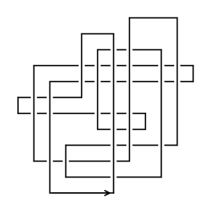
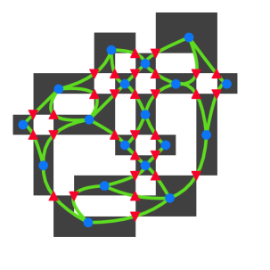
A knot can be oriented by choosing a direction along the strand. There are two ways to do this but they are equivalent. Each crossing obtains a twist sign according to the direction of the strands exiting the crossing; if the strands cross in a clockwise (counterclockwise) fashion then the crossing obtains a positive (negative) twist sign (see Fig.1(top-left)). The sum of all the twist signs is called writhe, , and characterises the knot chirality. The Jones polynomial is sensitive to the knot chirality as it can distinguish mirrored knots.
For any knot diagram, a planar graph called the Tait graph is defined as follows. The two-dimensional regions defined by the knot diagram can be bicoloured with, say, black and white, so that no two adjacent regions share a colour. There are two ways to do this, and so we choose the convention that the unique unbounded region (background) is white. In Fig.1 we show an example of a knot K (middle) along with its bicolouring (bottom). Then, vertices , where is the vertex set of , correspond to the black regions. Edges , where and is the edge set of , are such that they connect black regions through the knot diagram crossings. The graph thus obtained from is shown in Fig.1 (bottom), where vertices are represented by blue dots and edges by green lines. The vertex degree is denoted and counts the number of incident edges to that vertex. We have used the same symbol, , for crossings and the corresponding edges. The edges are decorated by Tait signs which are determined by the following rule. If the region to the left (right) is black when exiting a crossing on the over strand, then the crossing obtains a positive (negative) Tait sign (see Fig.1(top-right)). The sum of all tait signs is called Tait number, In Fig.1 (bottom), the Tait signs are represented by red triangles decorating the edges, pointing up(down) for positive(negative).
We now restate the relation between the -state PACI partition function and the Jones polynomial of a knot Chang and Shrock (2001); Wu and Wang (2001). A Potts model is placed on the Tait graph by defining spins with available states to reside on the vertices . The Tait signs that decorate the edges of G determine the interaction strength between spins, which take two corresponding values . This rule which assigns interactions between the -state spins renders the Potts model anisotropic. Their relation with the Jones variable is and the Jones variable is determined by fixing via Eq. (1). The Potts partition function over all spin-states is
| (2) | ||||
| (3) |
Multiplying the partition function with the appropriate prefactor , which accounts for twists and ensures that the unknot returns , we write
| (4) |
.
III Exact PACI partition function from tensor network contraction
Our goal is the evaluation of of PACI at some of our choice in order to use Eq.(4) and obtain the value of the Jones polynomial at as defined in Eq.(1). Note that computing the prefactor in Eq.(4) is in P as all , , are efficiently computable. Thus one would focus on computing as efficiently as possible.
However, the evaluation of on arbitrary graphs is a #P-hard problem Geraci and Lidar (2008). Regardless of this complexity, in this work we will use tensor network methods Kourtis et al. (2018) to obtain for Tait graphs exactly. From a graph we construct a tensor network encoding PACI as follows. Each vertex is endowed with a spin tensor (also known as a COPY tensor) of the form
| (5) |
which is a generalized -dimensional Kronecker tensor. Each edge obtains a vertex on which we place the interaction tensor of Eq. (3), which is always a matrix. Reinterpreting Fig.1 (bottom), we see the tensor network comprising and tensors (blue dots and red triangles respectively).
Full contraction of yields . This amounts to performing a sequence of tensor contractions, each being a dot product over the common index of two adjacent tensors in (green lines in Fig.1 (bottom). The partition function is then equivalently expressed as
| (6) |
Every contraction step yields a graph minor of the initial graph. Thus, when contracting a tensor network , there occurs at least one tensor of dimension equal to the maximal vertex degree over all minors .
In general, finding the optimal contraction sequence so that grows favourably slowly, is an NP-complete graph-theoretic problem Watanabe et al. (1983); Asano and Hirata (1983); Lewis and Yannakakis (1980); Belmonte et al. (2013). Practical contraction schemes for tensor networks is an active field of research Ran et al. (2017). We employ contraction methods introduced in Ref. Kourtis et al. (2018), where we refer the reader for explicit details of the methods, here dubbed greedy and METIS, which were developed for fast evaluation of partition functions similar to . In the greedy method, the “cheapest” edge contraction in terms of the resulting is performed. On the other hand, METIS heuristically constructs a separator hierarchy using the METIS algorithm Karypis and Kumar (1998), attempting to minimize the cut length while splitting the graph into comparably large components. The contraction is performed following the separator hierarchy in a coarse graining fashion. For details we point to Ref. Kourtis et al. (2018). We provide an example script demonstrating the evaluation of in an online repository ten .
III.1 Subexponential memory and runtime scaling
To investigate the performance of our numerical scheme, we require a procedure for generating random knots, whose Tait graphs we can use to evaluate the Jones polynomial. Since Tait graphs are planar and connected by construction, one may be tempted to just generate random connected planar graphs. However, not any planar connected graph corresponds to a knot shadow. A generic planar connected graph corresponds to a link shadow, where a link is viewed as the embedding of multiple nonintersecting components. Instead, we employ the random grid walk method Cromwell (1995); Even-Zohar (2017) to sample random knot diagrams, ensuring by construction that the number of components is always one. A grid walk consists of horizontal segments and vertical segments, where vertical segments always pass over horizontal ones. The walk is encoded by a random permutation of coordinates , where is the linear grid size, and steps of the form . Since all knots have a grid walk representation, any knot is accessible via this procedure. An example grid walk is shown in Fig. 1 (middle).
For a given orientation of the grid diagram, each crossing has a twist sign. All possible configurations are shown in Fig. 1 (top-left), and summing over them we obtain the writhe. The bicoloured knot along with its are shown Fig. 1 (bottom). Keeping in mind that vertical segments pass over horizontal ones, the colour pattern around a crossing determines the Tait signs , as shown in Fig. 1 (top-right), and so the Tait number is readily available.
With the random grid walk construction that allows us to randomly sample knots, we now investigate properties of the corresponding Tait graphs . First, we perform Reidemeister moves that leave the knot topology invariant but simplify the graph. In particular, a Reidemeister I introduces or removes a twist in the knot. We employ it to remove loops, i.e. edges of the form , as well as spikes, i.e,. degree- vertices, from the Tait graph. Note that a Reidemeister I move changes the writhe by . A Reidemeister II move amounts to overlaying a strand over or under another, or inversely, combing the strands so they do not cross. These moves are usually referred to as poke and unpoke, respectively. In terms of , we perform unpokes in order to remove double edges with . We then study the scaling of graph invariants of the resulting simplified graphs.
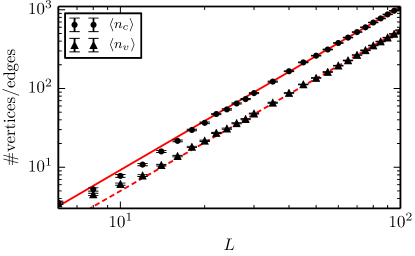
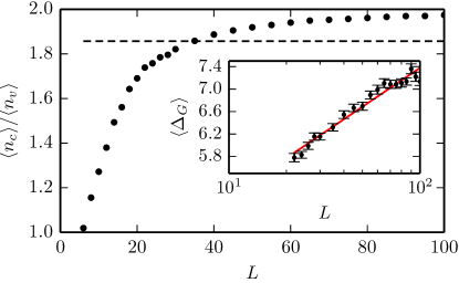
In Fig. 2 (top) we provide evidence for quadratic scaling of average number of vertices, , and average number of edges, , for simplified Tait graphs obtained by the random grid walk. In Fig. 2 (bottom) it is shown that the ratio of the average number of edges over the average number of vertices converges to as the size of the Tait graphs increases. This convergent behavior is compatible with the lower bound of this ratio for random planar graphs Stefanie et al. . Furthermore, for random planar graphs the average maximal degree , defined as , scales logarithmically with the graph size McDiarmid and Reed (2008). This is also confirmed for the simplified Tait graphs sampled by the random grid walk, as shown in Fig. 2 (inset). Note that the data presented in Fig. 2 are also a manifestation of the fact that the tensor networks, or equivalently, the interaction graphs of the PACI model relevant to the problem at hand, are irregular. This means that they are not amenable to efficient methods that yield the Potts model’s partition function on regular graphs, such as the Corner Transfer Matrix Renormalization Group in the case of the square lattice.
III.2 Numerical results
The central quantity of interest for the purposes of tensor network contraction is the maximal degree encountered in the sequence of minors occurring during contracting . This quantity characterizes the complexity of the algorithm, in the sense that runtime and memory requirements scale as .
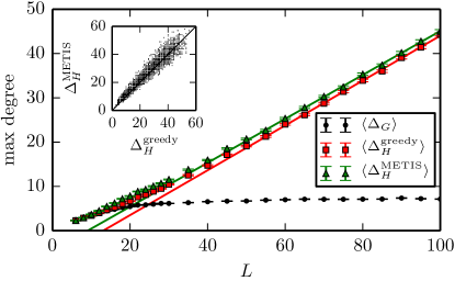
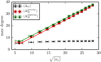
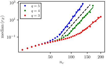
In Fig. 3 we show the scaling of the average with the grid-walk size . We find an asymptotically linear scaling with , which implies runtime scaling . Both contraction methods perform similarly, with METIS exhibiting marginally better scaling, yet only outperforming greedy for larger graphs (). We therefore use greedy to explicitly time the computation of for realistically accessible graph sizes. Runtime results for the cases of are shown in Fig. 4.
The favorable typical-case scaling allows us to evaluate the Jones polynomial for knots with for and with for , using moderate computational resources. For comparison, the largest calculations of the full expression for the Jones polynomial reported in the literature are for Hajij and Levitt (2018); Kno ; Sna ; Hoste and Thistlethwaite ; Deguchi and Tsurusaki (1993). Furthermore, for the exact evaluation of , we compare our algorithm’s -dependent performance with that of the -independent tree-decomposed transfer matrix algorithm (TDTM) Bedini and Jacobsen (2010), which in the literature is presented for random planar graphs of size up to . In Fig. 4 we show that for the greedy tensor network algorithm outperforms TDTM for typical instances.
The main bottleneck in these benchmarks is memory usage. For each there are exceptional knots that yield atypically large and thus evaluation of requires contraction of large tensors. With larger , these exceptional cases may overflow the available memory, even though typical cases with the same are easily amenable. On the other hand, for any particular knot of interest, one can test various graph contraction schemes to find the most favorable and thus gauge the resources required a priori. Then one can study typical cases alone, as we have demonstrated in Fig. 4, where for every we have obtained the runtimes for the graphs with .
Importantly, the asymptotic performance of our tensor network method does not depend on the content of the tensors, and so it is expected to perform as favorably for random planar instances of the Potts model, i.e. including those not corresponding to the Jones polynomial. Recall that Fig. 2 provides evidence that the graphs on which we have benchmarked our tensor network algorithm can be considered as random planar graphs. Therefore, and especially for the case of , this is a nontrivial result, as even incremental speedups in solving #P-hard problems are rare. We note that the slope change in the scaling of the median runtimes in Fig. 4 is likely due to the absence of CPU cache misses when tensor sizes remain small throughout the contraction of the network. We therefore disregard small systems below this slope change when we obtain runtime scalings.
IV Conclusions and outlook
In conclusion, we have developed a concrete methodology, based on tensor networks, for the evaluation of the Jones polynomial of arbitrary knots and demonstrated favorable performance of actual implementations. Due to the broad relevance of knot invariants, our methods have wide applicability: classification of knotted polymers Qin and Milner (2011), quantification of turbulence in classical and quantum fluids Ricca (2013), and study of the Jones conjecture Tuzun and Sikora (2016) are just a few examples of problems that require computation of knot polynomials. Furthermore, since Tait graphs are defined for links, our algorithm trivially can be extended to the study of links, as well. Recall that a link is the embedding of disjoint circles in with the knot as a special case. We therefore believe that the techniques introduced here can have multifaceted impact.
They also admit several extensions. For example, it is possible to obtain the coefficients of via polynomial interpolation between evaluations at a number of values of equal to the degree of , bounds to which are easily obtainable from the knot’s bicolouring(which is efficient) and scale polynomialy with the number of crossings Kauffman (2013). Moreover, in analogy with condensed matter applications of tensor networks, where truncation of singular values along edges of the network lead to accurate approximations of a desired physical quantity, appropriate truncation procedures may allow one to obtain controlled approximations of the Jones polynomial, and potentially other knot invariants. It is also interesting to consider whether our algorithms can be extended to cases of Gliozzi (2002); Hartmann (2005). Indeed, recall that the evaluation of corresponding to is a BQP-complete problem, except when corresponding to for which the problem is in P. This means that the quantum computation for the cases can be efficiently evaluated. Nevertheless, our algorithms are agnostic to the contents of the tensors and thus our results can extend to and be impactful for the study of the Potts model itself, as well as related graph theoretic problems such as -colouring, where the interactions decorating an interaction graph’s edge need not be compatible with the topology of a link diagram.
Acknowledgements.
We thank D. Aasen, G. Brennen, C. Chamon, P. Martin, A. Michailidis, J. Pachos, and Z. Papic for comments on the manuscript and inspiring discussions. S.K. was partially supported through the Boston University Center for Non-Equilibrium Systems and Computation. Preliminary numerical benchmarks were performed on the Boston University Shared Computing Cluster, which is administered by Boston University Research Computing Services. K.M. acknowledges the EPSRC Doctoral Prize Fellowship for financial support, J. K. Pachos for providing a workstation at the School of Physics & Astronomy, University of Leeds, and B. Coecke for providing access to the \textswabDuvel server at the Department of Computer Science, University of Oxford, where runtime results where obtained.References
- Kauffman (2013) Louis H. Kauffman, Knots and Physics, 4th ed. (World Scientific, 2013).
- Witten (1989) Edward Witten, “Quantum field theory and the Jones polynomial,” Comm. Math. Phys. 121, 351–399 (1989).
- Qin and Milner (2011) Jian Qin and Scott T. Milner, “Counting polymer knots to find the entanglement length,” Soft Matter 7, 10676 (2011).
- Enciso and Peralta-Salas (2013) Alberto Enciso and Daniel Peralta-Salas, “Knots and links in fluid mechanics,” Procedia IUTAM 7, 13 – 20 (2013), iUTAM Symposium on Topological Fluid Dynamics: Theory and Applications.
- Ricca (2013) Renzo L. Ricca, “Impulse of vortex knots from diagram projections,” Procedia IUTAM 7, 21 – 28 (2013), iUTAM Symposium on Topological Fluid Dynamics: Theory and Applications.
- Maggioni et al. (2013) Francesca Maggioni, Sultan Z. Alamri, Carlo F. Barenghi, and Renzo L. Ricca, “Vortex knots dynamics in euler fluids,” Procedia IUTAM 7, 29 – 38 (2013), iUTAM Symposium on Topological Fluid Dynamics: Theory and Applications.
- Liu and Ricca (2013) Xin Liu and Renzo L. Ricca, “Tackling fluid structures complexity by the Jones polynomial,” Procedia IUTAM 7, 175 – 182 (2013), iUTAM Symposium on Topological Fluid Dynamics: Theory and Applications.
- Cho et al. (2018) Y. M. Cho, Seung Hun Oh, and Pengming Zhang, “Knots in physics,” International Journal of Modern Physics A 33, 1830006 (2018).
- Wocjan and Yard (2006) Pawel Wocjan and Jon Yard, “The Jones polynomial: quantum algorithms and applications in quantum complexity theory,” arXiv:quant-ph/0603069 (2006), arXiv:0603069 [quant-ph] .
- Pachos (2012) Jiannis K. Pachos, Introduction to Topological Quantum Computation (Cambridge University Press, 2012).
- Mann and Bremner (2017) Ryan L. Mann and Michael J. Bremner, “On the complexity of random quantum computations and the jones polynomial,” (2017), arXiv:1711.00686 .
- Goldberg and Guo (2017) Leslie Ann Goldberg and Heng Guo, “The complexity of approximating complex-valued ising and tutte partition functions,” computational complexity 26, 765–833 (2017).
- Farhi et al. (2010) Edward Farhi, David Gosset, Avinatan Hassidim, Andrew Lutomirski, and Peter Shor, “Quantum money from knots,” (2010), arXiv:1004.5127 .
- Marzuoli and Palumbo (2011) Annalisa Marzuoli and Giandomenico Palumbo, “Post quantum cryptography from mutant prime knots,” International Journal of Geometric Methods in Modern Physics 08, 1571–1581 (2011).
- Horner et al. (2016) Kate E. Horner, Mark A. Miller, Jonathan W. Steed, and Paul M. Sutcliffe, “Knot theory in modern chemistry,” Chem. Soc. Rev. 45, 6432–6448 (2016).
- Klotz et al. (2018) Alexander R. Klotz, Beatrice W. Soh, and Patrick S. Doyle, “Motion of knots in dna stretched by elongational fields,” Phys. Rev. Lett. 120, 188003 (2018).
- Lim and Jackson (2015) Nicole C H Lim and Sophie E Jackson, “Molecular knots in biology and chemistry,” Journal of Physics: Condensed Matter 27, 354101 (2015).
- Mansfield (1994) Marc L. Mansfield, “Are there knots in proteins?” Nature Structural Biology 1, 213 EP – (1994).
- Raymer and Smith (2007) Dorian M. Raymer and Douglas E. Smith, “Spontaneous knotting of an agitated string,” Proceedings of the National Academy of Sciences 104, 16432–16437 (2007), http://www.pnas.org/content/104/42/16432.full.pdf .
- Birman and Hirsch (1998) Joan S. Birman and Michael D. Hirsch, “A new algorithm for recognizing the unknot,” (1998), 10.2140/gt.1998.2.175, arXiv:math/9801126 .
- Hass and Lagarias (1998) Joel Hass and Jeffrey C. Lagarias, “The number of reidemeister moves needed for unknotting,” (1998), arXiv:math/9807012 .
- Kuperberg (2011) Greg Kuperberg, “Knottedness is in NP, modulo GRH,” (2011), arXiv:1112.0845 .
- Lackenby (2013) Marc Lackenby, “A polynomial upper bound on reidemeister moves,” (2013), arXiv:1302.0180 .
- Jones (1985) Vaughan F. R. Jones, “A polynomial invariant for knots via von Neumann algebras,” Bull. Amer. Math. Soc. (N.S.) 12, 103–111 (1985).
- Hass et al. (1999) Joel Hass, Jeffrey C. Lagarias, and Nicholas Pippenger, “The computational complexity of knot and link problems,” J. ACM 46, 185–211 (1999).
- Kitaev (2003) A.Yu. Kitaev, “Fault-tolerant quantum computation by anyons,” Annals of Physics 303, 2 – 30 (2003).
- Jaeger et al. (1990) F. Jaeger, D. L. Vertigan, and D. J. A. Welsh, “On the computational complexity of the Jones and tutte polynomials,” Mathematical Proceedings of the Cambridge Philosophical Society 108, 35–53 (1990).
- Aharonov et al. (2005) Dorit Aharonov, Vaughan Jones, and Zeph Landau, “A polynomial quantum algorithm for approximating the Jones polynomial,” (2005), arXiv:quant-ph/0511096 .
- Iblisdir et al. (2014) S. Iblisdir, M. Cirio, O. Boada, and G.K. Brennen, “Low depth quantum circuits for ising models,” Annals of Physics 340, 205 – 251 (2014).
- Rowell and Wang (2017) Eric C. Rowell and Zhenghan Wang, “Mathematics of topological quantum computing,” (2017), arXiv:1705.06206 .
- Hajij and Levitt (2018) Mustafa Hajij and Jesse Levitt, “An efficient algorithm to compute the colored Jones polynomial,” (2018), arXiv:1804.07910 .
- (32) http://katlas.org/wiki/The_Mathematica_Package_KnotTheory .
- (33) https://www.math.uic.edu/t3m/SnapPy/ .
- (34) J Hoste and M Thistlethwaite, “Knotscape, a knot polynomial calculation program.” https://www.math.utk.edu/ morwen/knotscape.html .
- Deguchi and Tsurusaki (1993) Tetsuo Deguchi and Kyoichi Tsurusaki, “A new algorithm for numerical calculation of link invariants,” Physics Letters A 174, 29 – 37 (1993).
- El-Misiery and El-Horbaty (1996) A.E.M. El-Misiery and El-Sayed M. El-Horbaty, “An algorithm for calculating jones polynomials,” Applied Mathematics and Computation 74, 249 – 259 (1996).
- Wu (1992) F. Y. Wu, “Knot theory and statistical mechanics,” Rev. Mod. Phys. 64, 1099–1131 (1992).
- Wu (1982) F. Y. Wu, “The Potts model,” Rev. Mod. Phys. 54, 235–268 (1982).
- Graner and Glazier (1992) Fran çois Graner and James A. Glazier, “Simulation of biological cell sorting using a two-dimensional extended Potts model,” Phys. Rev. Lett. 69, 2013–2016 (1992).
- Levin and Nave (2007) M. Levin and C. P. Nave, “Tensor Renormalization Group Approach to Two-Dimensional Classical Lattice Models,” Phys. Rev. Lett. 99, 120601 (2007).
- Jiang et al. (2008) H. C. Jiang, Z. Y. Weng, and T. Xiang, “Accurate Determination of Tensor Network State of Quantum Lattice Models in Two Dimensions,” Phys. Rev. Lett. 101, 090603 (2008).
- Gu and Wen (2009) Z.-C. Gu and X.-G. Wen, “Tensor-entanglement-filtering renormalization approach and symmetry-protected topological order,” Phys. Rev. B 80, 155131 (2009).
- Xie et al. (2012) Z. Y. Xie, J. Chen, M. P. Qin, J. W. Zhu, L. P. Yang, and T. Xiang, “Coarse-graining renormalization by higher-order singular value decomposition,” Phys. Rev. B 86, 045139 (2012).
- Evenbly and Vidal (2015) G. Evenbly and G. Vidal, “Tensor Network Renormalization,” Phys. Rev. Lett. 115, 180405 (2015), arXiv:1412.0732 .
- Zhao et al. (2016) Hui-Hai Zhao, Z. Y. Xie, T. Xiang, and Masatoshi Imada, “Tensor network algorithm by coarse-graining tensor renormalization on finite periodic lattices,” Phys. Rev. B 93, 125115 (2016).
- Evenbly (2017) G. Evenbly, “Algorithms for tensor network renormalization,” Phys. Rev. B 95, 045117 (2017).
- Kourtis et al. (2018) Stefanos Kourtis, Claudio Chamon, Eduardo R. Mucciolo, and Andrei E. Ruckenstein, “Fast counting with tensor networks,” (2018), arXiv:1805.00475 .
- Chang and Shrock (2001) S.-C. Chang and R. Shrock, “Zeros of Jones polynomials for families of knots and links,” Physica A: Statistical Mechanics and its Applications 301, 196 – 218 (2001).
- Wu and Wang (2001) F.Y Wu and J Wang, “Zeroes of the Jones polynomial,” Physica A: Statistical Mechanics and its Applications 296, 483 – 494 (2001).
- Geraci and Lidar (2008) Joseph Geraci and Daniel A. Lidar, “On the exact evaluation of certain instances of the Potts partition function by quantum computers,” Communications in Mathematical Physics 279, 735–768 (2008).
- Watanabe et al. (1983) Toshimasa Watanabe, Tadashi Ae, and Akira Nakamura, “On the NP-hardness of edge-deletion and -contraction problems,” Discrete Applied Mathematics 6, 63 – 78 (1983).
- Asano and Hirata (1983) Takao Asano and Tomio Hirata, “Edge-contraction problems,” Journal of Computer and System Sciences 26, 197 – 208 (1983).
- Lewis and Yannakakis (1980) John M. Lewis and Mihalis Yannakakis, “The node-deletion problem for hereditary properties is NP-complete,” Journal of Computer and System Sciences 20, 219 – 230 (1980).
- Belmonte et al. (2013) Rémy Belmonte, Petr A. Golovach, Pim van ’t Hof, and Daniël Paulusma, “Parameterized Complexity of Two Edge Contraction Problems with Degree Constraints,” in Parameterized Exact Comput., edited by G. Gutin and S. Szeider (Springer, 2013) pp. 16–27.
- Ran et al. (2017) Shi-Ju Ran, Emanuele Tirrito, Cheng Peng, Xi Chen, Gang Su, and Maciej Lewenstein, “Review of tensor network contraction approaches,” (2017), arXiv:1708.09213 .
- Karypis and Kumar (1998) George Karypis and Vipin Kumar, “A Fast and High Quality Multilevel Scheme for Partitioning Irregular Graphs,” SIAM J. Sci. Comput. 20, 359–392 (1998).
- (57) https://gitlab.com/kourtis/tensorCSP .
- Cromwell (1995) Peter R. Cromwell, “Embedding knots and links in an open book I: Basic properties,” Topology and its Applications 64, 37–58 (1995).
- Even-Zohar (2017) Chaim Even-Zohar, “Models of random knots,” Journal of Applied and Computational Topology 1, 263–296 (2017).
- (60) Gerke Stefanie, Schlatter Dirk, Steger Angelika, and Taraz Anusch, “The random planar graph process,” Random Structures & Algorithms 32, 236–261, https://onlinelibrary.wiley.com/doi/pdf/10.1002/rsa.20186 .
- McDiarmid and Reed (2008) Colin McDiarmid and Bruce Reed, “On the maximum degree of a random planar graph,” Combinatorics, Probability and Computing 17, 591–601 (2008).
- Bedini and Jacobsen (2010) Andrea Bedini and Jesper Lykke Jacobsen, “A tree-decomposed transfer matrix for computing exact potts model partition functions for arbitrary graphs, with applications to planar graph colourings,” Journal of Physics A: Mathematical and Theoretical 43, 385001 (2010).
- Tuzun and Sikora (2016) Robert E. Tuzun and Adam S. Sikora, “Verification of the Jones unknot conjecture up to 22 crossings,” (2016), arXiv:1606.06671 .
- Gliozzi (2002) Ferdinando Gliozzi, “Simulation of Potts models with real q and no critical slowing down,” Phys. Rev. E 66, 016115 (2002).
- Hartmann (2005) A. K. Hartmann, “Calculation of partition functions by measuring component distributions,” Phys. Rev. Lett. 94, 050601 (2005).