PCA of high dimensional random walks with comparison to neural network training

Abstract

One technique to visualize the training of neural networks is to perform PCA on the parameters over the course of training and to project to the subspace spanned by the first few PCA components. In this paper we compare this technique to the PCA of a high dimensional random walk. We compute the eigenvalues and eigenvectors of the covariance of the trajectory and prove that in the long trajectory and high dimensional limit most of the variance is in the first few PCA components, and that the projection of the trajectory onto any subspace spanned by PCA components is a Lissajous curve. We generalize these results to a random walk with momentum and to an Ornstein-Uhlenbeck processes (i.e., a random walk in a quadratic potential) and show that in high dimensions the walk is not mean reverting, but will instead be trapped at a fixed distance from the minimum. We finally compare the distribution of PCA variances and the PCA projected training trajectories of a linear model trained on CIFAR-10 and ResNet-50-v2 trained on Imagenet and find that the distribution of PCA variances resembles a random walk with drift.

1 Introduction

Deep neural networks (NNs) are extremely high dimensional objects. A popular deep NN for image recognition tasks like ResNet-50 (He et al., 2016) has $\sim$25 million parameters, and it is common for language models to have more than one billion parameters (Jozefowicz et al., 2016). This overparameterization may be responsible for NNs impressive generalization performance (Novak et al., 2018). Simultaneously, the high dimensional nature of NNs makes them very difficult to reason about.

Over the decades of NN research, the common lore about the geometry of the loss landscape of NNs has changed dramatically. In the early days of NN research it was believed that NNs were difficult to train because they tended to get stuck in suboptimal local minima. Dauphin et al. (2014) and Choromanska et al. (2015) argued that this is unlikely to be a problem for most loss landscapes because local minima will tend not to be much worse than global minima. There are, however, many other plausible properties of the geometry of NN loss landscapes that could pose obstacles to NN optimization. These include: saddle points, vast plateaus where the gradient is very small, cliffs where the loss suddenly increases or decreases, winding canyons, and local maxima that must be navigated around.

Ideally we would like to be able to somehow visualize the loss landscapes of NNs, but this is a difficult, perhaps even futile, task because it involves embedding this extremely high dimensional space into very few dimensions — typically one or two. Goodfellow et al. (2014) introduced a visualization technique that consists of plotting the loss along a straight line from the initial point to the final point of training (the “royal road”). The authors found that the loss often decreased monotonically along this path. They further considered the loss in the space from the residuals between the NN’s trajectory to this royal road. Note that while this is a two-dimensional manifold, it is not a linear subspace. Lorch (2016) proposed another visualization technique in which principal component analysis (PCA) is performed on the NN trajectory and the trajectory is projected into the subspace spanned by the lowest PCA components. This technique was further explored by Li et al. (2018), who noted that most of the variance is in the first two PCA components.

In this paper we consider the theory behind this visualization technique. We show that PCA projections of random walks in flat space qualitatively have many of the same properties as projections of NN training trajectories. We then generalize these results to a random walk with momentum and a random walk in a quadratic potential, also known as an Ornstein-Uhlenbeck process (Uhlenbeck & Ornstein, 1930). This process is more similar to NN optimization since it consists of a deterministic component (the true gradient) plus a stochastic component. In fact, recent work has suggested that stochastic gradient descent (SGD) approximates a random walk in a quadratic potential (Ahn et al., 2012; Mandt et al., 2016; Smith & Le, 2017). Finally, we perform experiments on linear models and large NNs to show how closely they match this simplified model.

The approach we take to study the properties of the PCA of high dimensional random walks in flat space follows that of Moore & Ahmed (2017), but we correct several errors in their argument, notably in the values of the matrix $\textbf{S}^{T}\textbf{S}$ and the trace of $(\textbf{S}^{T}\textbf{S})^{-1}$ in Eq. 10. We also fill in some critical omissions, particularly the connection between banded Toeplitz matrices and circulant matrices. We extend their contribution by proving that the trajectories of high dimensional random walk in PCA subspaces are Lissajous curves and generalizing to random walks with momentum and Ornstein-Uhlenbeck processes.

2 PCA of random walks in flat space

2.1 Preliminaries

Let us consider a random walk in $d$-dimensional space consisting of $n$ steps where every step is equal to the previous step plus a sample from an arbitrary probability distribution, $\mathcal{P}$, with zero mean and a finite covariance matrix. For simplicity we shall assume that the covariance matrix has been normalized so that its trace is 1. This process can be written in the form

$$\textbf{x}_{t}=\textbf{x}_{t-1}+\bm{\xi}_{t},\qquad\bm{\xi}_{t}\sim\mathcal{P},$$ (1)

where $\textbf{x}_{t}$ is a $d$-dimensional vector and $\textbf{x}_{0}=\textbf{0}$. If we collect the $\textbf{x}_{t}$s together in an $n\times d$ dimensional design matrix X, we can then write this entire process in matrix form as

$$\textbf{S}\textbf{X}=\textbf{R},$$ (2)

where the matrix S is an $n\times n$ matrix consisting of 1 along the diagonal and -1 along the subdiagonal,

$$\textbf{S}\equiv\left(\begin{array}[]{rrrrr}1&0&0&\cdots&0\\ -1&1&0&\ddots&\vdots\\ 0&-1&1&\ddots&0\\ \vdots&\ddots&\ddots&\ddots&0\\ 0&\cdots&0&-1&1\\ \end{array}\right),$$ (3)

and the matrix R is an $n\times d$ matrix where every column is a sample from $\mathcal{P}$. Thus $\textbf{X}=\textbf{S}^{-1}\textbf{R}$.

To perform PCA, we need to compute the eigenvalues and eigenvectors of the covariance matrix $\hat{\textbf{X}}^{T}\hat{\textbf{X}}$, where $\hat{\textbf{X}}$ is the matrix X with the mean of every dimension across all steps subtracted. $\hat{\textbf{X}}$ can be found by applying the $n\times n$ centering matrix, C:

$$\hat{\textbf{X}}=\textbf{C}\textbf{X},\quad\textbf{C}\equiv\textbf{I}-\frac{1}{n}\textbf{1}\textbf{1}^{T}.$$ (4)

We now note that the analysis is simplified considerably by instead finding the eigenvalues and eigenvectors of the matrix $\hat{\textbf{X}}\hat{\textbf{X}}^{T}$. The non-zero eigenvalues of $\hat{\textbf{X}}^{T}\hat{\textbf{X}}$ are the same as those of $\hat{\textbf{X}}\hat{\textbf{X}}^{T}$. The eigenvectors are similarly related by $\textbf{v}_{k}=\textbf{X}^{T}\textbf{u}_{k}$, where $\textbf{v}_{k}$ is a (non-normalized) eigenvector of $\hat{\textbf{X}}^{T}\hat{\textbf{X}}$, and $\textbf{u}_{k}$ is the corresponding eigenvector of $\hat{\textbf{X}}\hat{\textbf{X}}^{T}$.

We therefore would like to find the eigenvalues and eigenvectors of the matrix

$$\hat{\textbf{X}}\hat{\textbf{X}}^{T}=\textbf{C}\textbf{S}^{-1}\textbf{R}\textbf{R}^{T}\textbf{S}^{-T}\textbf{C},$$ (5)

where we note that $\textbf{C}^{T}=\textbf{C}$. Consider the middle term, $\textbf{R}\textbf{R}^{T}$. In the limit $d\gg n$ we will have $\textbf{R}\textbf{R}^{T}\to\textbf{I}$ because the off diagonal terms will be $\mathbb{E}[\xi_{i}]^{2}=0$, whereas the diagonal terms will be $\mathbb{E}[\xi^{2}]=\sum_{i=0}^{d}\mathbb{V}[\xi_{i}]=1$. (Recall that we have assumed that the covariance of the noise distribution is normalized; if the covariance is not normalized, this simply introduces an overall scale factor given by the trace of the covariance.) We therefore have the simplification

$$\hat{\textbf{X}}\hat{\textbf{X}}^{T}=\textbf{C}\textbf{S}^{-1}\textbf{S}^{-T}\textbf{C}.$$ (6)

2.2 Asymptotic convergence to circulant matrices

Let us consider the new middle term, $\textbf{S}^{-1}\textbf{S}^{-T}=(\textbf{S}^{T}\textbf{S})^{-1}$. The matrix S is a banded Toeplitz matrix. Gray (2006) has shown that banded Toeplitz matrices asymptotically approach circulant matrices as the size of the matrix grows. In particular, Gray (2006) showed that banded Toeplitz matrices have the same inverses, eigenvalues, and eigenvectors as their corresponding circulant matrices in this asymptotic limit (see especially theorem 4.1 and subsequent material from Gray 2006). Thus in our case, if we consider the limit of a large number of steps, S asymptotically approaches a circulant matrix $\widetilde{\textbf{S}}$ that is equal to S in every entry except the top right, where there appears a $-1$ instead of a 0.

With the circulant limiting behavior of S in mind, the problem simplifies considerably. We note that C is also a circulant matrix, the product of two circulant matrices is circulant, the transpose of a circulant matrix is circulant, and the inverse of a circulant matrix is circulant. Thus the matrix $\hat{\textbf{X}}\hat{\textbf{X}}^{T}$ is asymptotically circulant as $n\to\infty$. Finding the eigenvectors is trivial because the eigenvectors of all circulant matrices are the Fourier modes. To find the eigenvalues we must explicitly consider the values of $\hat{\textbf{X}}\hat{\textbf{X}}^{T}$. The matrix $\textbf{S}^{T}\textbf{S}$ consists of a 2 along the diagonal, -1 along the subdiagonal and superdiagonal, and 0 elsewhere, with the exception of the bottom right corner where there appears a 1 instead of a 2.

While this matrix is not a banded Toeplitz, it is asymptotically equivalent to a banded Toeplitz matrix because it differs from a banded Toeplitz matrix by a finite amount in a single location. We now note that multiplication of the centering matrix does not change either the eigenvectors or the eigenvalues of this matrix since all vectors with zero mean are eigenvectors of the centering matrix with eigenvalue 1, and all Fourier modes but the first have zero mean. Thus the eigenvalues of $\hat{\textbf{X}}\hat{\textbf{X}}^{T}$ can be determined by the inverse of the non-zero eigenvalues of $\textbf{S}^{T}\textbf{S}$, which is an asymptotic circulant matrix. The $k^{\textrm{{th}}}$ eigenvalue of a circulant matrix with entries $c_{0},c_{1},\ldots$ in the first row is

$$\lambda_{\textrm{{circ}},k}=c_{0}+c_{n-1}\omega_{k}+c_{n-2}\omega_{k}^{2}+\ldots+c_{1}\omega_{k}^{n-1},$$ (7)

where $\omega_{k}$ is the $k^{\textrm{{th}}}$ root of unity. The imaginary parts of the roots of unity cancel out, leaving the $k^{\textrm{{th}}}$ eigenvalue of $\textbf{S}^{T}\textbf{S}$ to be

$$\lambda_{\textbf{S}^{T}\textbf{S},k}=2\left[1-\cos\left(\frac{\pi k}{n}\right)\right],$$ (8)

and the $k^{\textrm{{th}}}$ eigenvalue of $\hat{\textbf{X}}\hat{\textbf{X}}^{T}$ to be

$$\lambda_{\hat{\textbf{X}}\hat{\textbf{X}}^{T},k}=\frac{1}{2}\left[1-\cos\left(\frac{\pi k}{n}\right)\right]^{-1}.$$ (9)

The sum of the eigenvalues is given by the trace of $(\textbf{S}^{T}\textbf{S})^{-1}=\textbf{S}^{-1}\textbf{S}^{-T}$, and $\textbf{S}^{-1}$ is given by a lower triangular matrix with ones everywhere on and below the diagonal. The trace of $(\textbf{S}^{T}\textbf{S})^{-1}$ is therefore given by

$$\textrm{Tr}\left(\textbf{S}^{-1}\textbf{S}^{-T}\right)=\frac{1}{2}n(n+1),$$ (10)

and so the explained variance ratio from the $k^{\textrm{{th}}}$ PCA component, $\rho_{k}$ in the limit $n\to\infty$ is

$$\rho_{k}\equiv\frac{\lambda_{k}}{\textrm{Tr}\left(\textbf{S}^{-1}\textbf{S}^{-T}\right)}=\frac{\frac{1}{2}\left[1-\cos\left(\frac{\pi k}{n}\right)\right]^{-1}}{\frac{1}{2}n(n+1)}.$$ (11)

If we let $n\to\infty$ we can consider only the first term in a Taylor expansion of the cosine term. Requiring that $\sum_{k=1}^{\infty}\rho_{k}=1$, the explained variance ratio is

$$\rho_{k}=\frac{6}{\pi^{2}k^{2}}.$$ (12)

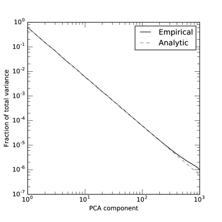
We test Eq. 12 empirically in Fig. 5 in the supplementary material.

We pause here to marvel that the explained variance ratio of a random walk in the limit of infinite dimensions is highly skewed towards the first few PCA components. Roughly 60% of the variance is explained by the first component, $\sim$80% by the first two components, $\sim$95% by the first 12 components, and $\sim$99% by the first 66 components.

2.3 Projection of the trajectory onto PCA components

Let us now turn to the trajectory of the random walk when projected onto the PCA components. The trajectory projected onto the $k^{\textrm{{th}}}$ PCA component is

$$\textbf{X}_{\textrm{{PCA}},k}=\textbf{X}\hat{\textbf{v}}_{k},$$ (13)

where $\hat{\textbf{v}}$ is the normalized $\textbf{v}_{k}$. We ignore the centering operation from here on because it changes neither the eigenvectors nor the eigenvalues. From above, we then have

$$\textbf{X}_{\textrm{{PCA}},k}=\frac{1}{\|\textbf{v}_{k}\|}\textbf{X}\textbf{v}_{k}=\frac{1}{\|\textbf{v}_{k}\|}\textbf{X}\textbf{X}^{T}\textbf{u}_{k}=\frac{\lambda_{k}}{\|\textbf{v}_{k}\|}\textbf{u}_{k}.$$ (14)

By the symmetry of the eigenvalue equations $\textbf{X}\textbf{X}^{T}\textbf{u}=\lambda\textbf{u}$ and $\textbf{X}^{T}\textbf{X}\textbf{v}=\lambda\textbf{v}$, it can be shown that

$$\|\textbf{v}_{k}\|=\|\textbf{X}^{T}\textbf{u}_{k}\|=\sqrt{\lambda}.$$ (15)

Since $\textbf{u}_{k}$ is simply the $k^{\textrm{{th}}}$ Fourier mode, we therefore have

$$\textbf{X}_{\textrm{{PCA}},k}=\sqrt{\frac{2\lambda_{k}}{n}}\cos\left(\frac{\pi kt}{n}\right).$$ (16)

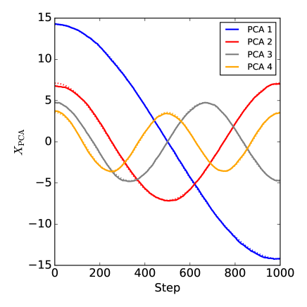
This implies that the random walk trajectory projected into the subspace spanned by two PCA components will be a Lissajous curve. In Fig. 1 we plot the trajectories of a high dimensional random walk projected to various PCA components and compare to the corresponding Lissajous curves. We perform 1000 steps of a random walk in 10,000 dimensions and find an excellent correspondence between the empirical and analytic trajectories. We additionally show the projection onto the first few PCA components over time in Fig. 6 in the supplementary material.

Figure 1: The PCA projections of the trajectories of high dimensional random walks are Lissajous curves. Left tableau: Projections of a 10,000-dimensional random walk onto various PCA components. Right tableau: Corresponding Lissajous curves from Eq. 16.

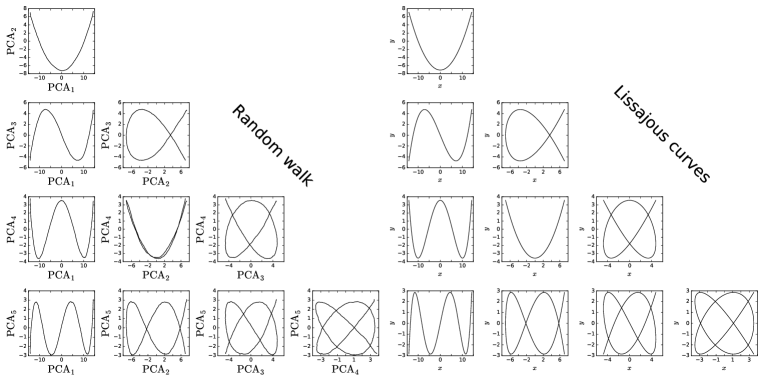
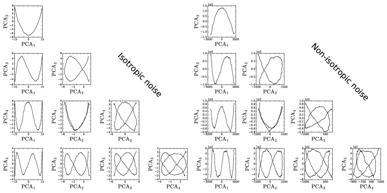
While our experiments thus far have used an isotropic Gaussian distribution for ease of computation, we emphasize that these results are completely general for any probability distribution with zero mean and a finite covariance matrix with rank much larger than the number of steps. We include the PCA projections and eigenvalue distributions of random walks using non-isotropic multivariate Gaussian distributions in Figs. 7 and 8 in the supplementary material.

3 Generalizations

3.1 Random walk with momentum

It is a common practice to train neural networks using stochastic gradient descent with momentum. It is therefore interesting to examine the case of a random walk with momentum. In this case, the process is governed by the following set of updates:

$$\textbf{v}_{t} = \gamma\textbf{v}_{t-1}+\bm{\xi}_{t}$$ (17)

$$\textbf{x}_{t} = \textbf{x}_{t-1}+\textbf{v}_{t}.$$ (18)

It can be seen that this modifies Eq. 2 to instead read

$$\textbf{S}\textbf{X}=\textbf{M}\textbf{R}$$ (19)

where M is a lower triangular Toeplitz matrix with 1 on the diagonal and $\gamma^{k}$ on the $k^{\textrm{{th}}}$ subdiagonal. The analysis from Section 2 is unchanged, except that now instead of considering the matrix $\textbf{S}^{-1}\textbf{S}^{-T}$ we have the matrix $\textbf{S}^{-1}\textbf{M}\textbf{M}^{T}\textbf{S}^{-T}$. Although M is not a banded Toeplitz matrix, its terms decay exponentially to zero for terms very far from the main diagonal. It is therefore asymptotically circulant as well, and the eigenvectors remain Fourier modes. To find the eigenvalues consider the product $(\textbf{S}^{T}\textbf{M}^{-T}\textbf{M}^{-1}\textbf{S})^{-1}$, noting that $\textbf{M}^{-1}$ is a matrix with 1s along the main diagonal and $-\gamma$s subdiagonal. With some tedious calculation it can be seen that the matrix $\textbf{S}^{T}\textbf{M}^{-T}\textbf{M}^{-1}\textbf{S}$ is given by

$$(\textbf{S}\textbf{M}^{-1}\textbf{M}^{-T}\textbf{S}^{T})_{ij}=\left\{\begin{array}[]{ll}2+2\gamma+\gamma^{2},&i=j\\ -(1+\gamma)^{2},&i=j\pm 1\\ \gamma,&i=j\pm 2\\ 0,&\textrm{otherwise}\end{array}\right.$$ (20)

with the exception that $\textbf{S}_{nn}=1$, and $\textbf{S}_{n,n-1}=\textbf{S}_{n-1,n}=-(1+\gamma)$. As before, this matrix is asymptotically circulant, so the eigenvalues of its inverse are

$$\lambda_{k}=\frac{1}{2}\left[1+\gamma+\gamma^{2}-(1+\gamma)^{2}\cos\left(\frac{\pi k}{n}\right)+\gamma\cos\left(\frac{2\pi k}{n}\right)\right]^{-1}.$$ (21)

In the limit of $n\to\infty$, the distribution of eigenvalues is identical to that of a random walk in flat space, however for finite $n$, it has the effect of shifting the distribution towards the lower PCA components. We empirically test Eq. 21 in Fig. 9 in the supplementary material.

3.2 Discrete Ornstein-Uhlenbeck processes

A useful generalization of the above analysis of random walks in flat space is to consider random walks in a quadratic potential, also known as an AR(1) process or a discrete Ornstein-Uhlenbeck process. For simplicity we will assume that the potential has its minimum at the origin. Now every step consists of a stochastic component and a deterministic component which points toward the origin and is proportional in magnitude to the distance from the origin. In this case the update equation can be written

$$\textbf{x}_{t}=(1-\alpha)\textbf{x}_{t-1}+\bm{\xi}_{t},$$ (22)

where $\alpha$ measures the strength of the potential. In the limit $\alpha\to 0$ the potential disappears and we recover a random walk in flat space. In the limit $\alpha\to 1$ the potential becomes infinitely strong and we recover independent samples from a multivariate Gaussian distribution. For $1<\alpha<2$ the steps will oscillate across the origin. For $\alpha$ outside $[0,2]$ the updates diverge exponentially.

3.2.1 Analysis of eigenvectors and eigenvalues

This analysis proceeds similarly to the analysis in Section 2 except that instead of S we now have the matrix $\textbf{S}_{\textrm{{OU}}}$ which has 1s along the diagonal and $-(1-\alpha)$ along the subdiagonal. $\textbf{S}_{\textrm{{OU}}}$ remains a banded Toeplitz matrix and so the arguments from Sec. 2 that $\hat{\textbf{{X}}}\hat{X}^{T}$ is asymptotically circulant hold. This implies that the eigenvectors of $\hat{\textbf{X}}\hat{\textbf{X}}^{T}$ are still Fourier modes. The eigenvalues will differ, however, because we now have that the components of $\textbf{S}_{\textrm{{OU}}}^{T}\textbf{S}_{\textrm{{OU}}}$ are given by

$$\left(\textbf{S}_{\textrm{{OU}}}^{T}\textbf{S}_{\textrm{{OU}}}\right)_{ij}=\left\{\begin{array}[]{ll}1+(1-\alpha)^{2},&i<n,i=j\\ -(1-\alpha),&i=j\pm 1\\ 1,&i=j=n\\ 0,&\textrm{otherwise.}\\ \end{array}\right.$$ (23)

From Eq. 7 we have that the $k^{\textrm{{th}}}$ eigenvalue of $\textbf{S}_{\textrm{{OU}}}^{T}\textbf{S}_{\textrm{{OU}}}$ is

$$\lambda_{\textrm{{OU}},k}=\left[1+(1-\alpha)^{2}-2(1-\alpha)\cos\left(\frac{2\pi k}{n}\right)\right]^{-1}\simeq\left[\frac{4\pi^{2}k^{2}(1-\alpha)}{n^{2}}+\alpha^{2}\right]^{-1}.$$ (24)

We show in Fig. 2 a comparison between the eigenvalue distribution predicted from Eq. 24 and the observed distribution from a 3000 step Ornstein-Uhlenbeck process in 30,000 dimensions for several values of $\alpha$. There is generally an extremely tight correspondence between the two. The exception is in the limit of $\alpha\to 1$, where there is a catch which we have hitherto neglected. While it is true that the mean eigenvalue of any eigenvector approaches the same constant, there is nevertheless going to be some distribution of eigenvalues for any finite walk. Because PCA sorts the eigenvalues, there will be a characteristic deviation from a flat distribution.

Figure 2: Left panel: The variance of the PCA components for several choices of $\alpha$. The empirical distribution is shown in solid and the predicted distribution with a dotted line. The predicted distribution generally matches the observed distribution closely, but there is a systematic deviation for $\alpha$ near 1. This is due to the fact that when the mean distribution is flat, there will nevertheless be a distribution around this mean when these eigenvalues are sampled from real data. Because PCA sorts these eigenvalues, this will always lead to a deviation from the flat distribution. Right panel: Distance from the origin for discrete Ornstein-Uhlenbeck processes with several choices of $\alpha$ (solid lines) with the predicted asymptote from Eq. 25 (dotted lines).

3.2.2 Critical distance and mixing time

While we might be tempted to take the limit $n\to\infty$ as we did in the case of a random walk in flat space, doing so would obscure interesting dynamics early in the walk. (A random walk in flat space is self-similar so we lose no information by taking this limit. This is no longer the case in an Ornstein- Uhlenbeck process because the parameter $\alpha$ sets a characteristic scale in the system.) In fact there will be two distinct phases of a high dimensional Ornstein-Uhlenbeck process initialized at the origin. In the first phase the process will behave as a random walk in flat space — the distance from the origin will increase proportionally to $\sqrt{n}$ and the variance of the $k^{\textrm{{th}}}$ PCA component will be proportional to $k^{-2}$. However, once the distance from the origin reaches a critical value, the gradient toward the origin will become large enough to balance the tendency of the random walk to drift away from the origin. At this point the trajectory will wander indefinitely around a sphere centered at the origin with radius given by this critical distance. Thus, while an Ornstein-Uhlenbeck process is mean-reverting in low dimensions, in the limit of infinite dimensions the Ornstein-Uhlenbeck process is no longer mean-reverting — an infinite dimensional Ornstein-Uhlenbeck process will never return to its mean. This critical distance can be calculated by noting that each dimension is independent of every other and it is well known that the asymptotic distribution of an AR(1) process with Gaussian noise is Gaussian with a mean of zero and a standard deviation of $\sqrt{V/(1-(1-\alpha)^{2})}$, where $V$ is the variance of the stochastic component of the process. In high dimensions the asymptotic distribution as $n\to\infty$ is simply a multidimensional isotropic Gaussian. Because we are assuming $V=1/d$, the overwhelming majority of points sampled from this distribution will be in a narrow annulus at a distance

$$r_{c}=\frac{1}{\sqrt{\alpha(2-\alpha)}}$$ (25)

from the origin. Since the distance from the origin during the initial random walk phase grows as $\sqrt{n}$, the process will start to deviate from a random walk after $n_{c}\sim(\alpha(2-\alpha))^{-1}$ steps. We show in the right panel of Fig. 2 the distance from the origin over time for 3000 steps of Ornstein-Uhlenbeck processes in 30,000 dimensions with several different choices of $\alpha$. We compare to the prediction of Eq. 25 and find a good match.

3.2.3 Iterate averages converge slowly

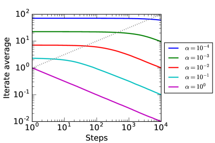
We finally note that if the location of the minimum is unknown, then iterate (or Polyak) averaging can be used to provide a better estimate. But the number of steps must be much greater than $n_{c}$ before iterate averaging will improve the estimate. Only then will the location on the sphere be approximately orthogonal to its original location on the sphere and the variance on the estimate of the minimum will decrease as $1/\sqrt{n}$. We compute the mean of converged Ornstein-Uhlenbeck processes with various choices of $\alpha$ in Fig. 10 in the supplementary material.

3.2.4 Random walks in non-isotropic potential are dominated by low curvature directions

While our analysis has been focused on the special case of a quadratic potential with equal curvature in all dimensions, a more realistic quadratic potential will have a distribution of curvatures and the axes of the potential may not be aligned with the coordinate basis. Fortunately these complications do not change the overall picture much. For a general quadratic potential described by a positive semi-definite matrix $A$, we can decompose $A$ into its eigenvalues and eigenvectors. We then apply a coordinate transformation to align the parameter space with the eigenvectors of $A$. At this point we have a distribution of curvatures, each one given by an eigenvalue of $A$. However, because we are considering the limit of infinite dimensions, we can assume that there will be a large number of dimensions that fall in any bin $[\alpha_{i},\alpha_{i}+d\alpha]$. Each of these bins can be treated as an independent high-dimensional Ornstein-Uhlenbeck process with curvature $\alpha_{i}$. After $n$ steps, PCA will then be dominated by dimensions for which $\alpha_{i}$ is small enough that $n\ll n_{c,i}$. Thus, even if relatively few dimensions have small curvature they will come to dominate the PCA projected trajectory after enough steps.

4 Comparison to linear models and neural networks

While random walks and Ornstein-Uhlenbeck processes are analytically tractable, there are several important differences between these simple processes and optimization of even linear models. In particular, the statistics of the noise will depend on the location in parameter space and so will change over the course of training. Furthermore, there may be finite data or finite trajectory length effects.

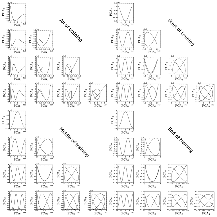
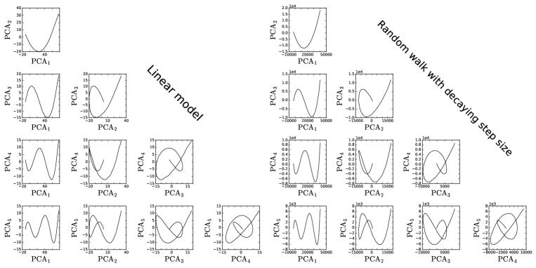
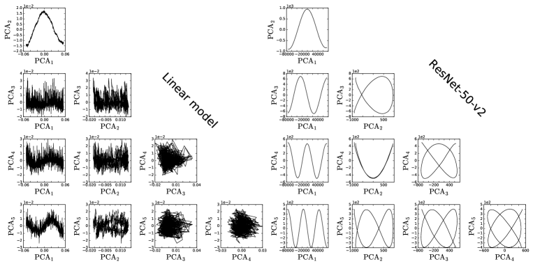
To get a sense for the effect of these differences we now compare the distribution of the variances in the PCA components between two models and a random walk. For our first model we train a linear model without biases on CIFAR-10 using a learning rate of $10^{-5}$ for 10,000 steps. For our second model we train ResNet-50-v2 on Imagenet without batch normalization for 150,000 steps using SGD with momentum and linear learning rate decay. We collect the value of all parameters at every step for the first 1500 steps, the middle 1500 steps, and the last 1500 steps of training, along with collecting the parameters every 100 steps throughout the entirety of training. Further details of both models and the training procedures can be found in the supplementary material. While PCA is tractable on a linear model of CIFAR-10, ResNet-50-v2 has $\sim$25 million parameters and performing PCA directly on the parameters is infeasible, so we instead perform a random Gaussian projection into a subspace of 30,000 dimensions. We show in Fig. 3 the distribution of the PCA variances at the beginning, middle, and end of training for both models and compare to the distribution of variances from an infinite dimensional random walk. We show tableaux of the PCA projected trajectories from the middle of training for the linear model and ResNet-50-v2 in Fig. 4. Tableaux of the other training trajectories in various PCA subspaces are shown in the supplementary material.

The distribution of eigenvalues of the linear model resembles an OU process, whereas the distribution of eigenvalues of ResNet-50-v2 resembles a random walk with a large drift term. The trajectories appear almost identical to those of random walks shown in Fig. 1, with the exception that there is more variance along the first PCA component than in the random walk case, particularly at the start and end points. This manifests itself in a small outward turn of the edges of the parabola in the PCA2 vs. PCA1 projection. This suggests that ResNet-50-v2 generally moves in a consistent direction over relatively long spans of training, similarly to an Ornstein-Uhlenbeck process initialized beyond $r_{c}$.

Figure 3: Left panel: The distribution of PCA variances at various points in training for a linear model trained on CIFAR-10. At the beginning of training the model’s trajectory is more directed than a random walk, as exhibited by the steep distribution in the lower PCA components. By the middle of training this distribution has flattened (apart from the first PCA component) and more closely resembles that of an Ornstein-Uhlenbeck process. Right panel: The distribution of PCA variances of the parameters of ResNet-50-v2 at various points in training. The distribution of PCA variances generally matches that of a random walk with the exception of the first PCA component, which dominates the distribution, particularly at the end of training.

Figure 4: Left tableau: PCA projected trajectories from the middle of training a linear model on CIFAR-10. Training has largely converged at this point, producing an approximately Gaussian distribution in the higher PCA components. Right tableau: PCA projected trajectories from the middle of training ResNet-50-v2 on Imagenet. These trajectories strongly resemble those of a random walk. See Figs. 12 and 13 in the supplementary material for PCA projected trajectories at other phases of training.

5 Random walks with decaying step sizes

We finally note that the PCA projected trajectories of the linear model and ResNet-50-v2 over the entire course of training qualitatively resemble those of a high dimensional random walk with exponentially decaying step sizes. To show this we train a linear regression model $y=\textbf{W}\textbf{x}$, where W is a fixed, unknown vector of dimension 10,000. We sample x from a 10,000 dimensional isotropic Gaussian and calculate the loss

$$\mathcal{L}=\frac{1}{2}(y-y^{\prime})^{2},$$ (26)

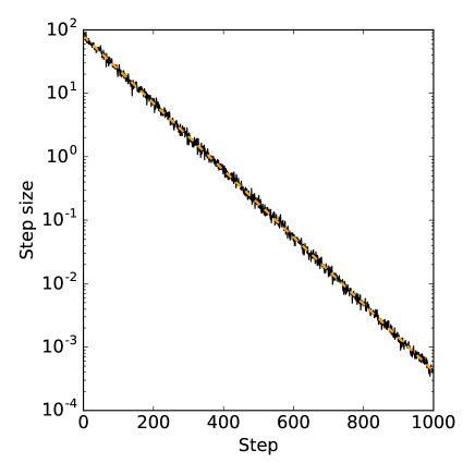
where $y^{\prime}$ is the correct output. We show in Fig. 14 that the step size decays exponentially. We fit the decay rate to this data and then perform a random walk in 10,000 dimensions but decay the variance of the stochastic term $\bm{\xi}_{i}$ by this rate. We compare in Fig. 15 of the supplementary material the PCA projected trajectories of the linear model trained on synthetic data to the decayed random walk. We note that these trajectories resemble the PCA trajectories over the entire course of training observed in Figs. 12 and 13 for the linear model trained on CIFAR-10 and ResNet-50-v2 trained on Imagenet.

6 Conclusions

We have derived the distribution of the variances of the PCA components of a random walk both with and without momentum in the limit of infinite dimensions, and proved that the PCA projections of the trajectory are Lissajous curves. We have argued that the PCA projected trajectory of a random walk in a general quadratic potential will be dominated by the dimensions with the smallest curvatures where they will appear similar to a random walk in flat space. Finally, we find that the PCA projections of the training trajectory of a layer in ResNet-50-v2 qualitatively resemble those of a high dimensional random walk despite the many differences between the optimization of a large NN and a high dimensional random walk.

Acknowledgments

The authors thank Matthew Hoffman, Martin Wattenberg, Jeffrey Pennington, Roy Frostig, and Niru Maheswaranathan for helpful discussions and comments on drafts of the manuscript.

7 Further empirical tests

7.1 High dimensional random walks

We test Eq. 12 by computing 1000 steps of a random walk in 10,000 dimensions and performing PCA on the trajectory. We show in Fig. 5 the empirical variance ratio for the various components compared to the prediction from Eq. 12 and find excellent agreement. The empirical variance ratio is slightly higher than the predicted variance ratio for the highest PCA components due to the fact that there are a finite number of dimensions in this experiment, so the contribution from all components greater than the number of steps taken must be redistributed among the other components, which leads to proportionally the largest increase in the largest PCA components.

Figure 5: The fraction of the total variance of the different PCA components for a high dimensional random walk. The solid line is calculated from performing PCA on a 10,000 dimensional random walk of 1000 steps. The dashed line is calculated from the analytic prediction of Eq. 12. There is excellent agreement up until the very largest PCA components where finite size effects start to become non-negligible.

We show in Fig. 6 the projection of the trajectory onto the first few PCA components. The projection onto the $k^{\textrm{{th}}}$ PCA component is a cosine of frequency $k/(2n)$ and amplitude given by Eq. 12.

Figure 6: The projection of the trajectory of a high-dimensional random walk onto the first five PCA components forms cosines of increasing frequency and decreasing amplitude. The predicted trajectories are shown with dotted lines, but the difference between the predicted and observed trajectories is generally smaller than the width of the lines. The random walk in this figure consists of 1000 steps in 10,000 dimensions.

7.2 Random walk with non-isotropic noise

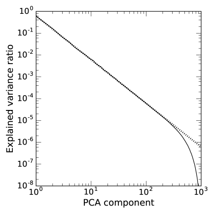
To demonstrate that our results hold for non-isotropic noise distributions we perform a random walk where the noise is sampled from a multivariate Gaussian distribution with a random covariance matrix, $\bm{\Sigma}$. Because sampling from a multivariate Gaussian with an arbitrary covariance matrix is difficult in high dimensions, we restrict the random walk to 1000 dimensions, keeping the number of steps 1000 as before. To construct the covariance matrix, we sample a $1000\times 1000$ dimensional random matrix, R, where each element is a sample from a normal distribution and then set $\bm{\Sigma}=\textbf{R}\textbf{R}^{T}$. Although $\bm{\Sigma}$ will be approximately equal to the identity matrix, the distribution of eigenvalues will follow a fairly wide Marchenko-Pastur distribution because R is square. We show the distribution of explained variance ratios with the prediction from Eq. 12 in Fig. 7. There is a tight correspondence between the two up until the largest PCA components where finite dimension effects start to dominate. We also show in Fig. 8 PCA projected trajectories of this random walk along with a random walk where the random variates are sampled from a 1000-dimensional isotropic distribution for comparison to provide a sense for the amount of noise introduced by the relatively small number of dimensions. Although the small dimensionality introduces noise into the PCA projected trajectories, it is clear that the general shapes match the predicted Lissajous curves.

Figure 7: The distribution of explained variance ratios from the PCA of a random walk with noise sampled from a multivariate Gaussian with a non- isotropic covariance matrix. Despite the different noise distribution, the distribution of explained variance ratios closely matches the prediction from Eq. 12.

Figure 8: Left tableau: The PCA projected trajectory of a random walk with noise sampled from an isotropic Gaussian distribution in 1000 dimensions. Right tableau: The PCA projected trajectory of a random walk with noise sampled from a multivariate Gaussian distribution with a random covariance matrix in 1000 dimensions. Although the smaller number of dimensions introduces noise into the trajectory, it is clear that the trajectories are still Lissajous curves even when the random variates are sampled from a more complicated distribution.

7.3 Random walk with momentum

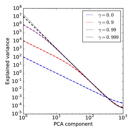
We test Eq. 21 by computing 1000 steps of a random walk in 10,000 dimensions with various choices of the momentum parameter, $\gamma$. We show in Fig. 9 the observed distribution of PCA variances (not the explained variance ratio) along with the prediction from Eq. 21. There is an extremely tight correspondence between the two, except for the lowest PCA components for $\gamma=0.999$. This is expected because the effective step size is set by $n/(1-\gamma)$, and because $n=1000$, the walk does not have sufficient time to settle into its stationary distribution of eigenvalues when $\gamma=0.999$.

Figure 9: The distribution of explained PCA variances for random walks with momentum where we vary the strength of the momentum parameter, $\gamma$. The distribution observed from a 1000 step random walk in 10,000 dimensions is shown in the solid lines. The prediction from Eq. 21 is shown in the dashed line.

7.4 Iterate averaging of an Ornstein-Uhlenbeck process

We show in Fig. 10 the mean of all steps of Ornstein-Uhlenbeck processes which have converged to a random walk on a sphere of radius $r_{c}$. We show in the dashed line the predicted value of $n_{c}$, the number of steps required to reach $r_{c}$ (i.e., the crossing time of the sphere). The position on the sphere will close to its original location for $n\ll n_{c}$ so iterate averaging will not improve the estimate of the minimum. Only when $n\gg n_{c}$ will iterate averaging improve the estimate of the minimum since the correlation between new points wit the original location will be negligible.

Figure 10: The mean of all steps of converged Ornstein-Uhlenbeck processes of various lengths. The mean remains approximately constant until the total angle from the initial position on the sphere grows to $\sim$$\pi/2$, which requires $\sim$$\alpha^{-1}$ steps (dashed line).

8 Details of models and training

8.1 Linear regression on CIFAR-10

We train linear regression on CIFAR-10 for 10,000 steps using SGD and a batch size of 128 and a learning rate of $10^{-5}$. The model achieves a validation accuracy of 29.1%.

8.2 ResNet-50-v2 on Imagenet

We train ResNet-50-v2 on Imagenet for 150,000 steps using SGD with momentum and a batch size of 1024. We do not use batch normalization since this could confound our analysis of the training trajectory. We instead add bias terms to every convolutional layer. We decay the learning rate linearly with an initial learning rate of 0.0345769 to a final learning rate a factor of 10 lower by 141,553 steps, at which point we keep the learning rate constant. We set the momentum to 0.9842. The network achieves a validation accuracy of 71.46%.

9 Gallery of PCA projected trajectories

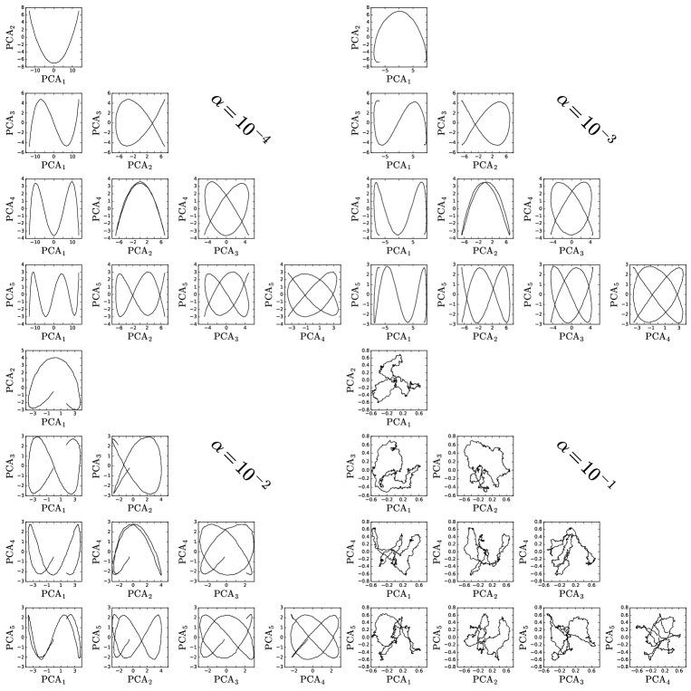
We present here tableaux of the PCA projections of various trajectories. We show in Fig. 11 four tableaux of the PCA projections of the trajectories of high-dimensional Ornstein-Uhlenbeck processes with different values of $\alpha$. For $\alpha=10^{-4}$ the trajectories are almost identical to a high-dimensional random walk, as they should be since the process was sampled for only 1000 steps. Once we have $\alpha^{-1}=1000$ the trajectories start to visibly deviate from those of a high-dimensional random walk. For larger $\alpha$ the deviations continue to grow until they become unrecognizable at $\alpha=0.1$ because 1000 steps corresponds to many crossing times on the high dimensional sphere on which the process takes place.

Figure 11: Tableaux of the PCA projections of the trajectories of high-dimensional Ornstein-Uhlenbeck processes with various values of $\alpha$. All processes were sampled for 1000 steps in 10,000 dimensions. Upper left tableau: $\alpha=10^{-4}$. Upper right tableau: $\alpha=10^{-3}$. Lower left tableau: $\alpha=10^{-2}$. Lower right tableau: $\alpha=10^{-1}$.

In Fig. 12 we present tableaux of the PCA projections of the linear model trained on CIFAR-10. The trajectory of the entire training process somewhat resembles a high-dimensional random walk, though because the model makes larger updates at earlier steps than at later ones there are long tails on the PCA projected trajectories. The model’s trajectory most closely resembles a high-dimensional random walk early in training, but towards the end the higher components become dominated by noise, implying that these components more closely resemble a converged Ornstein-Uhlenbeck process. This corresponds with the flattening of the distribution of eigenvalues in Fig. 3.

Figure 12: Tableaux of the trajectories of a linear model trained on CIFAR-10 in different PCA subspaces. Upper left tableau: PCA applied to every tenth step over all of training. Upper right tableau: PCA applied to the first 1000 steps of training. Lower left tableau: PCA applied to the middle 1000 steps of training. Lower right tableau: PCA applied to the last 1000 steps of training.

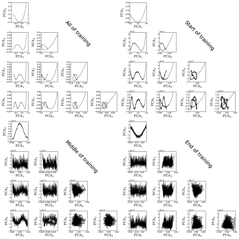
In Fig. 13 we present tableaux of the PCA projections of ResNet-50-v2 trained on Imagenet. Perhaps remarkably, these trajectories resemble a high-dimensional random walk much more closely than the linear model. However, as in the case of the linear model, the resemblance deteriorates later in training.

Figure 13: Tableaux of the parameter trajectories of ResNet-50-v2 trained on Imagenet in different PCA subspaces. The parameters were first projected into a random Gaussian subspace with 30,000 dimensions before PCA was applied. Upper left tableau: PCA applied to every hundredth step over all of training. Upper right tableau: PCA applied to the first 1500 steps of training. Lower left tableau: PCA applied to the middle 1500 steps of training. Lower right tableau: PCA applied to the last 1500 steps of training.

Figure 14: The change in the step size from training a linear model on synthetic Gaussian data. The step size decays exponentially with the best fit shown in the orange dashed line.

Figure 15: Left tableau: PCA projected trajectories of a linear regression model trained on synthetic Gaussian data. Right tableau: PCA projected trajectories of a 10,000 dimensional random walk where the variance of the stochastic component is decayed using the best fit found from the linear regression model trained on synthetic data. The trajectories in the two tableaux appear very similar.

References

- Ahn et al. (2012) Ahn, Sungjin, Korattikara, Anoop, and Welling, Max. Bayesian posterior sampling via stochastic gradient fisher scoring. arXiv preprint arXiv:1206.6380, 2012.
- Choromanska et al. (2015) Choromanska, Anna, Henaff, Mikael, Mathieu, Michael, Arous, Gérard Ben, and LeCun, Yann. The loss surfaces of multilayer networks. In Artificial Intelligence and Statistics, pp. 192–204, 2015.
- Dauphin et al. (2014) Dauphin, Yann N, Pascanu, Razvan, Gulcehre, Caglar, Cho, Kyunghyun, Ganguli, Surya, and Bengio, Yoshua. Identifying and attacking the saddle point problem in high-dimensional non-convex optimization. In Advances in neural information processing systems, pp. 2933–2941, 2014.
- Goodfellow et al. (2014) Goodfellow, Ian J, Vinyals, Oriol, and Saxe, Andrew M. Qualitatively characterizing neural network optimization problems. arXiv preprint arXiv:1412.6544, 2014.
- Gray (2006) Gray, Robert M. Toeplitz and circulant matrices: A review. Foundations and Trends® in Communications and Information Theory, 2(3):155–239, 2006.
- He et al. (2016) He, Kaiming, Zhang, Xiangyu, Ren, Shaoqing, and Sun, Jian. Deep residual learning for image recognition. In Proceedings of the IEEE conference on computer vision and pattern recognition, pp. 770–778, 2016.
- Jozefowicz et al. (2016) Jozefowicz, Rafal, Vinyals, Oriol, Schuster, Mike, Shazeer, Noam, and Wu, Yonghui. Exploring the limits of language modeling. arXiv preprint arXiv:1602.02410, 2016.
- Li et al. (2018) Li, Hao, Xu, Zheng, Taylor, Gavin, Studor, Christoph, and Goldstein, Tom. Visualizing the loss landscape of neural nets. In International Conference on Learning Representations, 2018.
- Lorch (2016) Lorch, Eliana. Visualizing deep network training trajectories with pca. In ICML Workshop on Visualization for Deep Learning, 2016.
- Mandt et al. (2016) Mandt, Stephan, Hoffman, Matthew, and Blei, David. A variational analysis of stochastic gradient algorithms. In International Conference on Machine Learning, pp. 354–363, 2016.
- Moore & Ahmed (2017) Moore, James and Ahmed, Hasan. High dimensional random walks can appear low dimensional: Application to influenza h3n2 evolution. arXiv preprint arXiv:1707.09361, 2017.
- Novak et al. (2018) Novak, Roman, Bahri, Yasaman, Abolafia, Daniel A, Pennington, Jeffrey, and Sohl-Dickstein, Jascha. Sensitivity and generalization in neural networks: an empirical study. International Conference on Learning Representations, 2018.
- Smith & Le (2017) Smith, Samuel L and Le, Quoc V. A bayesian perspective on generalization and stochastic gradient descent. In Proceedings of Second workshop on Bayesian Deep Learning (NIPS 2017), 2017.
- Uhlenbeck & Ornstein (1930) Uhlenbeck, George E and Ornstein, Leonard S. On the theory of the brownian motion. Physical review, 36(5):823, 1930.