Deep Sequence Learning with Auxiliary Information
for Traffic Prediction

Abstract.

Predicting traffic conditions from online route queries is a challenging task as there are many complicated interactions over the roads and crowds involved. In this paper, we intend to improve traffic prediction by appropriate integration of three kinds of implicit but essential factors encoded in auxiliary information. We do this within an encoder-decoder sequence learning framework that integrates the following data: 1) offline geographical and social attributes. For example, the geographical structure of roads or public social events such as national celebrations; 2) road intersection information. In general, traffic congestion occurs at major junctions; 3) online crowd queries. For example, when many online queries issued for the same destination due to a public performance, the traffic around the destination will potentially become heavier at this location after a while. Qualitative and quantitative experiments on a real-world dataset from Baidu have demonstrated the effectiveness of our framework.

1. Introduction

Traffic prediction is an important part of intelligent transportation systems (ITS) and is crucial to many applications including traffic network planning, route guidance, and congestion avoidance (Zhang et al., 2011). For large cities such as Beijing, such prediction is crucial but challenging to perform. This is due to the dynamic and complex traffic environment in large cities and the limited potential for new roads: this places an important emphasis on network management. Such management has a wide-reaching impact, not just due to the large population involved, but also because it supports decision making in various other applications e.g. the optimization of pollution is relevant to traffic. In this paper, we argue that previous models have failed to effectively include several important factors for prediction. We outline these as follows, before introducing our system which utilises these and demonstrates a positive impact on our application.

Offline geographical and social factors. The geographical structure of roads has an impact on traffic dynamics. For example, the traffic on a main road would be different from that of a lane and in general traffic congestion occurs more often at a major junction. Furthermore, social temporal factors such as holidays and the weekend have an influence on traffic. These characteristics serve to highlight the difficulty of traffic prediction.

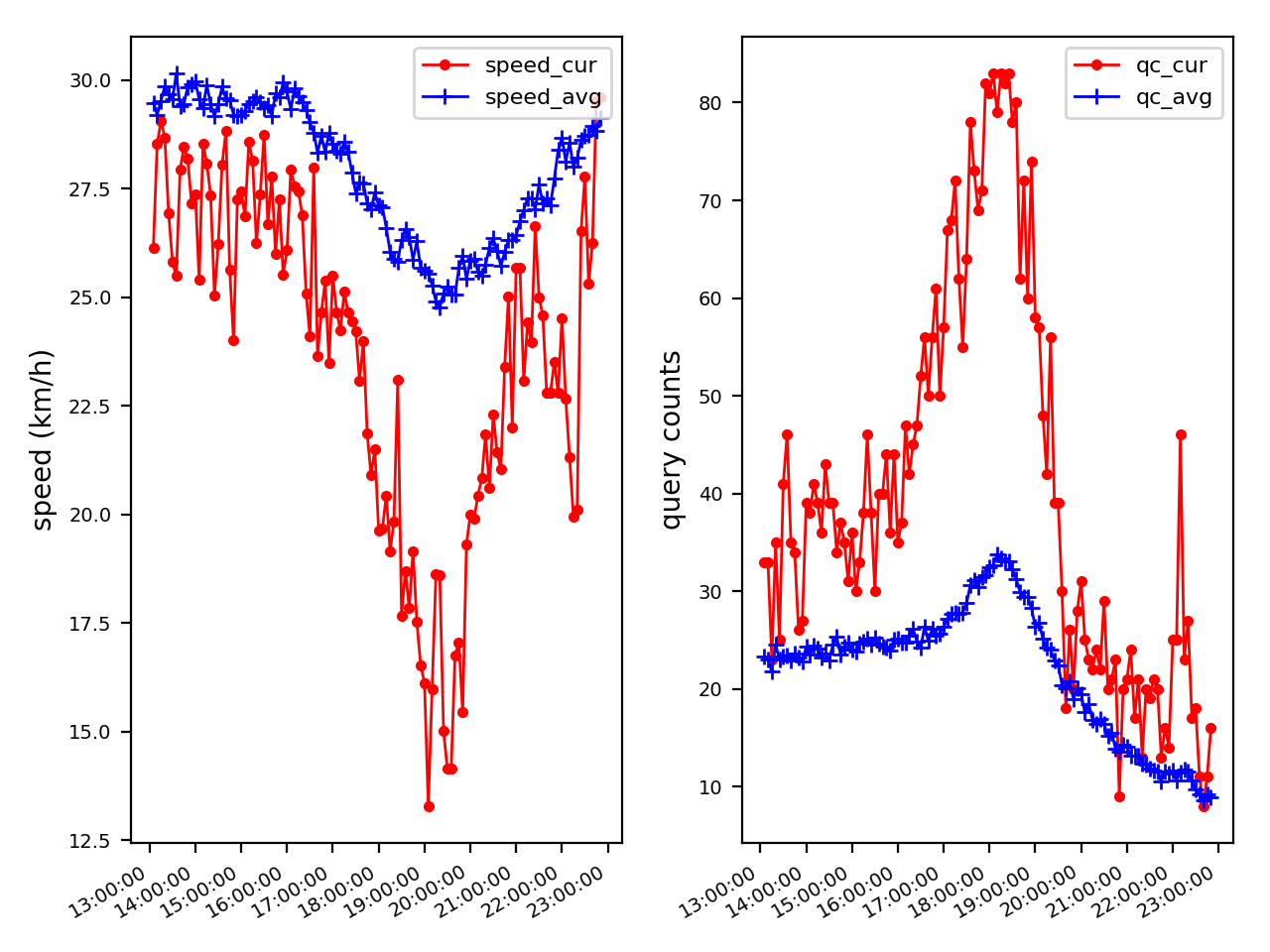
Online potential influence. Widely used mobile technology applications such as Baidu Map and Google Map provide a rich source of data for transportation analysis and forecasting. Figure 1 shows the average traffic speed and crowd query counts around Capital Gym, Beijing on April 8, 2017. The query counts at time $t$ are calculated by accumulating the queries whose destinations are around Capital Gym and their estimated arrival time is $t$. We can clearly observe that the current query counts (in red) are much more than usual query counts (in blue) at 18:00, which leads to a sudden drop of the traffic speed. Note that the query is long-term (the average travel time is 46 minutes shown in Table 2) foreseeable, which would provide an early warning of traffic jams in ITS. More interestingly, the emergence of map queries from the crowd indicates that there is an event here, namely “Fish Leong Concert”. Online map queries from the crowd, which are innately related to the future states of road networks, can potentially be used to predict traffic dynamics, making the integration of multi-modal data an interesting yet challenging problem.

Limited dataset. Due to the accessibility of traffic data, previous research on traffic prediction usually use limited datasets for experimentation. There are relatively few publicly available large-scale traffic prediction datasets for researchers to compare their models and propose new models.

Figure 1. The traffic speed (left) and online query counts (right) around the Beijing Capital Gym on April 8, 2017. The red line denotes the unusual traffic speed (query counts) while the blue line indicates the usual traffic speed (query counts). At 19:00 PM, there was the Fish Leong Concert in the Capital Gym.

To improve the state of the art in traffic prediction, we release a large-scale traffic dataset from Baidu Map, the Q-Traffic dataset, which provides various offline and online auxiliary information along with traffic speed data. There are three kinds of auxiliary domains in the Q-Traffic dataset: 1) Offline geographical and social attributes which include public holidays, peak-hour, speed etc; 2) the road intersection information such as local road network and junctions; and 3) online crowd queries which record map search queries from users.

Table 4 shows that the offline geographical and social attributes from the Q-traffic dataset include a large number of categorical features, making the input features space sparse, i.e., the field speedclass contains 8 class of speed limit. Learning and exploiting the sparse feature through a wide feature transformation is effective and interpretable, but requires a large degree of feature engineering effort. Conversely, deep neural networks can generalize better through low-dimensional dense embeddings. Motivated by (Cheng et al., 2016), a wide transformation is utilised to learn the interactions from the sparse geographical and social attributes while an encoder-decoder deep network is used to decode the traffic condition given the combination of the traffic encoding and transformed features.

Furthermore, due to the spatial dependencies in the road network, it is natural to utilise the graph convolutional neural networks (Niepert et al., 2016) to embed the traffic conditions induced by neighbouring road segments. Specifically, given a central road segment, neighbouring road segments are selected based on the PageRank score (Page et al., 1999) at first, which measures local spatial importance. The combination of graph CNN and the encoder-decoder deep network can integrate spatial patterns and historical traffic sequence.

Online map queries from the crowd, which are innately related to the future states of road networks, would potentially influence the traffic condition. For example, assume that we had the historical traffic data of road segments around the Capital Gym by 17:00 PM, being aware of many people would arrive at the Beijing Capital Gym around 18:00 PM, would effectively boost the performance of traffic prediction at 18:00 PM. We quantify the potential impact that online crowd queries have on the road segments, embed the impact with an encoder, and assemble the traffic and query impact with a deep fusion.

In this paper, we effectively utilise three kinds of auxiliary information in an encoder-decoder sequence to sequence (Seq2Seq) (Cho et al., 2014; Sutskever et al., 2014) learning manner as follows: a wide linear model is used to encode the interactions among geographical and social attributes, a graph convolution neural network is used to learn the spatial correlation of road segments, and the query impact is quantified and encoded to learn the potential influence of online crowd queries. Therefore a hybrid model based on deep sequence learning with auxiliary information for traffic prediction is proposed. In this model, offline geographical and social attributes, spatial dependencies and online crowd queries are integrated. The contribution of this paper can be summarised as follows:

• We release a large-scale traffic prediction dataset with offline and online auxiliary information including map crowd search queries, road intersections and geographical and social attributes.

• We integrate the sequence to sequence deep neural networks with geographical and social attributes via a wide and deep manner.

• To incorporate the spatial dependencies within local road network, we utilise the graph convolution neural network to embed the traffic speed of neighbouring road segments.

• We quantify the potential influence and devise a query impact algorithm to calculate the impact that online crowd queries have on the road segments.

• We propose a hybrid Seq2Seq model which incorporates the offline geographical and social attributes, spatial dependencies and online crowd queries with a deep fusion.

The rest of this paper is organised as follows. We first introduce the released dataset in Sec.2. Following that, we propose a series of methods for traffic prediction on the Q-Traffic dataset in Sec.3. Sec.4 presents qualitative and quantitative results of different methods. Sec.5 presents the related work of traffic prediction. Finally, we conclude the paper in Sec.6.

2. Q-Traffic Dataset

In this section, we first introduce a large-scale traffic prediction dataset — Q-Traffic dataset , which consists of three sub-datasets: query sub-dataset, traffic speed sub-dataset and road network sub-dataset. We compare our released Q-Traffic dataset with different datasets used for traffic prediction.

Table 1. Examples of discovered events, where Time, Grid, QC_cur, QC_last, Top1 query word, Top1_qc, and Description represents the start time and end time, grid coordinates, query counts in the current time period, query counts in the same period of last week, top 1 query word, top 1 query counts and the description of each event, respectively.

Time	Grid	QC_cur	QC_last	Top1 query word	Top1_qc	Description
2017-04-08 14:00-20:00	(26, 39)	3431	417	Capital Gym	2724	Fish Leong Concert
2017-04-11 08:00-10:00	(24, 38)	447	93	Beijing Shangri-La Restaurant	304	IBM Data Scientist Forum
2017-04-15 08:00-16:00	(13, 47)	4551	2202	Beijing Botanical Garden	3849	Spring outing
2017-04-15 16:00-20:00	(21, 34)	2173	207	Letv sports center	1831	Chou Chuan-huing Concert
2017-04-30 08:00-18:00	(22, 47)	7283	3607	Summer Palace	7149	Summer Palace (May Day)
2017-04-30 08:00-18:00	(26, 46)	3691	1582	Tsinghua University	3102	106th Anniversary of THU

2.1. Query Sub-dataset

Figure 2. The flowchart of the mining of potential traffic in queries. A set of map queries is segmented into grids, then we can estimate the arrival time at each query’s destination, thus constructing an arrival time tensor. An event discovery algorithm is used to discover the events from the arrival time tensor.

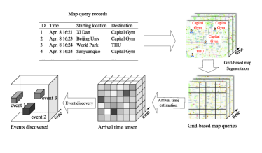
This sub-dataset was collected in Beijing, China between April 1, 2017 and May 31, 2017, from the Baidu Map application. Two modes of map queries are provided by the Baidu Map: one is called “location search”, which includes the searches of a specific place; the other is called “route search”, which recommends a navigation route from one location to another. This sub-dataset contains about 114 million user queries, each of which records the user ID (anonymised), search time-stamp, coordinate of the current location, coordinate and query word of starting location (in “route search”), coordinate and query word of destination. Note that if the query mode is “location search”, the starting location is the same as the current location. The top/left of the Figure 2 shows several records of the query sub-dataset. This dataset is pre-processed as follows, with the statistics of the dataset after processing given in Table 2.

• To eliminate redundancy, only the last query will be retained if a single user submitted several queries in 10 minutes.

• The queries whose current locations are 2km (or more) away from the starting locations will be eliminated due to the assumption that the users are more likely to go to their searched destinations if they are currently close to the searched starting location.

• Since the filtered starting locations are all within 2km from current locations, the starting time is estimated according to the distance between starting location and current location, with a speed of 3.6km/h (by walk).

• As shown in Figure 2, the map is partitioned into a $R\times C$ grid map according to the lon/lat bounding box of (116.10, 39.69, 116.71, 40.18), where $R=72,C=68$ and the width and height of a grid are both about 1km.

• For each query, since the exact time when the user arrives at the destination is not available, an estimated arrival time $t_{d}^{i}$ for “route search” is calculated according to the query mode with a speed of 30km/h (by car), 20km/h (by bus), 10km/h (by bike) or 3.6km/h (by walk). And the estimated arrival time $t_{d}^{i}$ for “location search” is calculated according to the distance between the starting location and destination, with a speed of 20km/h (by bus, distance $>$ 2km) or 3.6km/h (by walk, distance $\leq$ 2km).

A query $q^{i}$ can be represented as $q^{i}=(t_{s}^{i},s^{i},d^{i},x_{s}^{i},y_{s}^{i},x_{d}^{i},y_{d}^{i})$ where $i=1,2,\dots,n$. We can calculate $(x_{s}^{i},y_{s}^{i},x_{d}^{i},y_{d}^{i})$ based on the grid map, where $t_{s}^{i}$, $t_{d}^{i}$, $s^{i}$, $d^{i}$, $(x_{s}^{i},y_{s}^{i})$, $(x_{d}^{i},y_{d}^{i})$, $n$ stand for the starting time-stamp, estimated arrival time, query word of the starting location, query word of the destination, coordinates of the starting location and the destination, and the number of all queries, respectively.

Table 2. Statistics of the query sub-dataset in Beijing between April 1 and May 31, 2017.

Items	#
Filtered queries	114,658,750
Query words	17,210,732
Average distance/query	12km
Average travel time/query	46 minutes

We note that a user may not go to the destination that they have searched, however, they will be much more likely to go to this destination if it relates to a public event that is occurring. To account for this, we declare an “event” (see Sec.2.1.1) to have occurred when query counts for a place are much higher than usual over a short period of time. For example, assume that we had received a lot of queries for Capital Gym as a destination and the arrival time was around 6 PM on April 8, 2017. As the number of queries is much more than usual we postulate that there could be an “event” here (in this case the “Fish Leong Concert”). The users who submitted these queries have a high probability of going to the Capital Gym for the concert. For all queries $\bm{Q}=\{q^{i}|i=1,2,\dots,n\}$, we can construct arrival time tensor $\bm{D}=\{d_{x,y,t}\}$, where $x=1,2,\dots,C$, $y=1,2,\dots,R$, $t=1,2,\dots,T$, and $T=5,856$ ($61\text{-day}\times 24\text{-hour}\times 4\text{-quarter}$) is the total time-stamps (since we aggregate the queries every 15 minutes). We define $d_{x,y,t}$ as:

(1) $$d_{x,y,t}=|\{q^{k}|x_{d}^{k}=x,y_{d}^{k}=y,t_{d}^{k}=t\}|$$

where $|\cdot|$ denotes the cardinality of a set. We will use the arrival time tensor $\bm{D}$ to discover the events in Sec.2.1.1 .

2.1.1. Event Discovery

The density $\rho_{d}=\frac{N}{R\times C\times T}$ of arrival time tensor $\bm{D}$ is 4, which implies $\bm{D}$ is very sparse. We will find the spatiotemporal ranges whose query counts are much more than usual, using the following definitions.

Definition 2.1 (Moment).

A tuple $m=(x,y,t)$ is a moment if

(2) $$d_{x,y,t-\Delta t}>0$$

(3) $$d_{x,y,t}-d_{x,y,t-\Delta t}>\zeta$$

(4) $$\frac{d_{x,y,t}-d_{x,y,t-\Delta t}}{d_{x,y,t-\Delta t}}>\eta$$

We denote $\mathcal{M}$ a set of all moments.

Definition 2.2 (Event).

A tuple $E=(x,y,t_{s},t_{d})$ is an event if

(5) $$t_{d}-t_{s}>\epsilon$$

(6) $$\forall t\in[t_{s},t_{d}],\quad m=(x,y,t)\in\mathcal{M}$$

(7) $$m=(x,y,t_{s}-1)\not\in\mathcal{M}\land m=(x,y,t_{d}+1)\not\in\mathcal{M}$$

According to the Def.2.1 and Def.2.2, let $\eta=0.2$, $\zeta=300$, $\Delta t=672$ ($7\times 24\times 4$, a week), $\epsilon=4$ (an hour), 932 events are discovered. The number of all the event queries and time steps is 2,336,114 and 15,892, respectively. Thus the density $\rho_{e}$ of all the events is 147, which is much larger than $\rho_{d}=4$. Table 1 shows some events that we discovered. Several kinds of events are presented, including concerts, forums, places of interest and anniversaries. For each event, one can find that the query counts are much more than that in last week, and the top 1 query word is highly related to the event. Not only that, more than 80% of the query counts comes from the top 1 query word.

2.2. Traffic Speed Sub-dataset

Figure 3. Spatial distribution of the road segments in Beijing

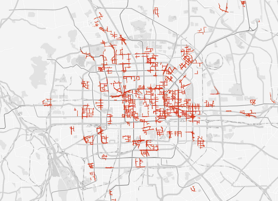
We also collect the traffic speed data for the same area and during the same time period as the query sub-dataset. The origin traffic speed dataset contains the traffic speed of $\sim$450k road segments. What we are interested in are the traffic conditions of those road segments which are close to the events. Thus we collect a sub-dataset whose road segments are nearby the destinations where events held. This sub-dataset contains 15,073 road segments covering approximately 738.91 km. Table 3 and Figure 3 shows the statistics and spatial distribution of these road segments, respectively. They are all in the 6th ring road, which is the most crowded area of Beijing. The traffic speed of each road segment is recorded per minute. Since the traffic speed sub-dataset is from real-world urban areas, the traffic lights would have a great impact on the traffic speed, leading to the traffic speed varies greatly. For instance, the traffic speed may differ 20km/h between two consecutive minutes. To make the traffic speed predictable, for each road segment, we use simple moving average with a 15-minute time window to smooth the traffic speed sub-dataset and sample the traffic speed per 15 minutes.

Table 3. Statistics of the traffic speed sub-dataset

Items	#
Road segments	15,073
Total length	738.91 km
Interval	15 minutes
Time	April 1, 2017 - May 31, 2017
Total records	265,967,808
lon/lat bounding box	(116.10, 39.69, 116.71, 40.18)

Table 4. Examples of geographical attributes of each road segment.

Field	Type	Description
link_id	Char (13)	road segment id
width	Char (3)	width, 15: ¡=3.0m; 30: (3.0m, 5.0m);
		55: (5.5m, 13m); 130: ¿13m
direction	Char (1)	direction, 0: unknown, default two-way;
		1: two-way; 2: single-way, from start
		node to end node; 3: single-way, from
		end node to start node
snodeid	Char (13)	start node id
enodeid	Char (13)	end node id
snodegps	Char (30)	gps coordinate (lon, lat) of start node
enodegps	Char (30)	gps coordinate (lon, lat) of end node
length	Char (8)	length (kilo-meter)
speedclass	Char (1)	speed limit (km/h), 1: ¿130; 2: (100, 130);
		3: (90, 100); 4: (70, 90); 5: (50, 70);
		6: (30, 50); 7: (11, 30); 8: ¡11
lanenum	Char (1)	number of lanes, 1: 1; 2: 2 or 3; 3: ¿=4

Table 5. Comparison of different datasets for traffic speed prediction.

Datasets	Scale	Road info.	Road net.	Auxiliary info.	Highway	Urban	Available
Subset of PeMS			$\surd$		$\surd$		$\surd$
State Route 22, Garden Grove (Yang et al., 2017)	9
PeMSD7 (S) (Yu et al., 2017)	228
San Francisco Bay area (He et al., 2013)	943
PeMSD7 (L) (Yu et al., 2017)	1,026
Subset of Beijing			$\surd$
Ring road around Beijing (Ma et al., 2015)	2					$\surd$
Beijing 4th ring road (Tang et al., 2017)	3					$\surd$
Beijing 2nd/3rd ring road (Wang et al., 2016)	80				$\surd$
Beijing 2nd/3rd ring road (Wang et al., 2016)	122				$\surd$
Bejing taxi dataset (Ma et al., 2017)	236				$\surd$	$\surd$
Bejing taxi dataset (Ma et al., 2017)	352				$\surd$	$\surd$
I-80 in California (Duan et al., 2016)	6		$\surd$		$\surd$		$\surd$
Busan Metropolitan City (Kim et al., 2016)	10		$\surd$			$\surd$
California PATH (Bezuglov and Comert, 2016)	12				$\surd$
Corridor in Orlando (Qi and Ishak, 2014)	71				$\surd$
Rome dataset (Fusco et al., 2016)	120		$\surd$			$\surd$
D100 (Gülaçar et al., 2016)	122			weather		$\surd$
Bedok area (Dauwels et al., 2014)	226		$\surd$		$\surd$	$\surd$
Los Angeles (Deng et al., 2016)	1,642		$\surd$		$\surd$	$\surd$
Los Angeles (Deng et al., 2016)	4,048		$\surd$		$\surd$	$\surd$
Dallas-Forth Worth area (Hasanzadeh et al., 2017)	4,764				$\surd$
Subnetwork in Singapore (Asif et al., 2014)	5,024		$\surd$		$\surd$	$\surd$
Q-Traffic Dataset	15,073	$\surd$	$\surd$	map query	$\surd$	$\surd$	$\surd$

2.3. Road Network Sub-dataset

Due to the spatiotemporal dependencies of traffic data, the topology of the road network would help to predict traffic. Table 4 shows the fields of the road network sub-dataset. For each road segment in the traffic speed sub-dataset, the road network sub-dataset provides the starting node (snode) and ending node (enode) of the road segment, based on which the topology of the road network can be built. In addition, the sub-dataset also provides various geographical attributes of each road segment, such as width, length, speed limit and the number of lanes. Furthermore, we also provide the social attributes such as weekdays, weekends, public holidays, peak hours and off-peak hours.

2.4. Comparison with Other Datasets

Table 5 shows the comparison of different datasets for traffic speed prediction. The most popular dataset for traffic prediction is Caltrans Performance Measurement System (PeMS). However, it doesn’t provide road attributes and other auxiliary information. In the past few years, researchers have performed experiments with small or (and) private datasets. The release of Q-Traffic, a large-scale public available dataset with offline (geographical and social attributes, road network) and online (crowd map queries) information, should lead to an improvement of the research of traffic prediction.

3. Methodologies

In this section, we will introduce the definition of traffic speed prediction problem and the hybrid model to integrate three auxiliary domains one by one.

3.1. Problem Definition

In a mere temporal model, the prediction of traffic speed can be formalised as forecasting future traffic speed $\{\bm{v}_{t+1},\bm{v}_{t+2},\dots,\bm{v}_{t+t^{\prime}}\}$ given previous traffic speed $\{\bm{v}_{1},\bm{v}_{2},\dots,\bm{v}_{t}\}$. The Q-Traffic dataset makes it possible to combine benefits from multiple auxiliary domains including spatial relation within local road network, offline geographical and social attributes and online crowd search queries.

Figure 4. Seq2Seq: The Sequence to Sequence model predicts future traffic speed $\{\tilde{\bm{v}}_{t+1},\tilde{\bm{v}}_{t+2},\dots,\tilde{\bm{v}}_{t+t^{\prime}}\}$, given the previous traffic speed $\{\bm{v}_{1},\bm{v}_{2},...\bm{v}_{t}\}$.

3.2. Seq2Seq

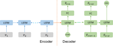
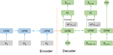
The fundamental network to be applied on the Q-Traffic for mere temporal patterns is the Sequence to Sequence (Seq2Seq) model (Cho et al., 2014; Sutskever et al., 2014). Both the encoder and decoder can be constructed based on LSTM (Hochreiter and Schmidhuber, 1997). The Seq2Seq model with LSTM has achieved a great success on different tasks such as speech recognition (Graves and Jaitly, 2014), machine translation (Sutskever et al., 2014) and video question answering (Venugopalan et al., 2015).

Figure 4 shows the architecture of the Seq2Seq model for traffic prediction. The encoder embeds the input traffic speed sequence $\{\bm{v}_{1},\bm{v}_{2},\dots,\bm{v}_{t}\}$ and the final hidden state of the encoder is fed into the decoder, which learns to predict the future traffic speed $\{\tilde{\bm{v}}_{t+1},\tilde{\bm{v}}_{t+2},\dots,\tilde{\bm{v}}_{t+t^{\prime}}\}$. Hybrid model that integrates the auxiliary information will be proposed based on the Seq2Seq model.

Figure 5. Seq2Seq + Attributes: The model incorporates offline geographical and social attributes $\{\bm{AT}(\bm{v}_{t+1}),\bm{AT}(\bm{v}_{t+2}),\dots,\bm{AT}(\bm{v}_{t+t^{\prime}})\}$ into the decoder of the Seq2Seq model.

3.3. Seq2Seq + Attributes

As aforementioned, it is beneficial to introduce both geographical and social attributes into traffic sequence learning instead of merely utilising speed information.

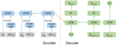
There are two kinds of offline attributes that have been extracted for wide and deep learning. 1) Geographical attributes including width, direction, speed limit and the number of lanes of each road segment (Table 4). 2) Social attributes including information on public holidays, workdays, peak hours and off-peak hours.

Motivated by (Cheng et al., 2016), we utilise a wide and deep network that combine the benefits from deep learning and feature engineering. These attributes $\bm{AT}(\bm{v}_{t})$ are concatenated directly into the decoder network of the Seq2Seq model and the encoder network remains identical as shown in Figure 5.

Figure 6. Seq2Seq + Spatial Relation: Traffic speed of neighbouring road segments $\{\bm{NB}(\bm{v}_{1}),\bm{NB}(\bm{v}_{2}),\dots,\bm{NB}(\bm{v}_{t})\}$ is embedded into the encoder of Seq2Seq model by using Graph Convolutional Neural Network. The neighbouring road segements are selected based on PageRank score, which reflects impact of neighbours on the central road segment.

3.4. Seq2Seq + Spatial Relation

The traffic at a specific road segment can be affected by its neighbouring road segments (Yu et al., 2017). However, the Seq2Seq model is designed to learn temporal dependencies but not spatial dependencies within road intersections.

Graph Convolutional Neural Networks (Niepert et al., 2016) are applied to embed traffic of neighbouring road segments, $\bm{NB}(\bm{v}_{t})$, into the encoder of the Seq2Seq model as shown in Figure 6. As each road segment has a direction of traffic flow, the local road intersections can be constructed as a directed graph. Given a central road segment, five predecessors and five successors in the directed graph are selected based on PageRank score (Page et al., 1999), which provides the relative spatial impact of neighbouring road segments on the central road segment.

3.5. Seq2Seq + Query Impact

Correlation Analysis. The query counts have a clear correlation with the traffic speed. For each event, we compute the average traffic speed of all the road segments within a range of 1km and measure the correlation between the average traffic speed and the corresponding query counts with a resolution of 15 minutes. As both of the variables are non-linear, Spearman’s rank correlation coefficient is applied and the result $\rho=-0.52$ with a $P$-value$=1.23\times 10^{-4}$ indicates a strong negative correlation between the average traffic speed and the query counts, making the prediction of traffic with the query sub-dataset promising.

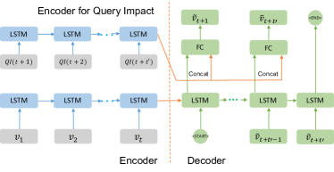
Query Impact. The query impact $\bm{QI}$ measures the influence of queries on road segments. It is calculated based on the query counts and the spatial region that the query will influence.

Given an event at location $A$, note that the queries come from different places $\{S_{1},S_{2},...\}$, each query has different impact on different road segments around the location $A$. Thus, the query impact should consider the spatial locations of each query. As described in Section 2.1, let $Q=\{q^{i}|i=1,2,\dots,n\}$ denotes all the queries, where $q^{i}=(t_{s}^{i},t_{d}^{i},s^{i},d^{i},x_{s}^{i},y_{s}^{i},x_{d}^{i},y_{d}^{i})$. Road segments are denoted by $RS=\{l^{i}|i=1,2,\dots,k\}$. The query impact $\bm{QI(l,t)}$ of queries on each road segments $l$ can be calculated by Algorithm 1. In the Algorithm 1, the function $dist$ in line 10 calculates the Euclidean distance of a point and a segment. The $h$ in line 11 is a decreasing function whose input is the distance $d_{l}$ and output is the impact $h(d_{l})$ that query $q^{i}$ makes on the road segment $l$ at time $t_{d}^{i}$. For simplicity, we choose the exponential function $h(x)=exp(-\frac{x}{\sigma})$, where $\sigma$ is the impact factor.

Input: A set $Q=\{q^{1},q^{2},\dots,q^{n}\}$ of queries, where $q^{i}=(t_{s}^{i},t_{d}^{i},s^{i},d^{i},x_{s}^{i},y_{s}^{i},x_{d}^{i},y_{d}^{i})$, a set $RS=\{l^{1},l^{2},\dots,l^{k}\}$ of links, total time stamp $T$

Output: The query impact QI

1 Initialisation: $QI(l,t)\leftarrow 0$

2 for $i\leftarrow 1$ to $n$ do

3       // return the longitude and latitude of a location

4       $lonlat_{s}\leftarrow lonlat(s^{i})$

5       $lonlat_{d}\leftarrow lonlat(d^{i})$

6       $seg_{i}\leftarrow segment(lonlat_{s},lonlat_{d})$

7       // return the set of road segments within 1km $L\leftarrow nearroad(lonlat_{d})$

8       for each $l\in L$ do

9             $lonlat_{l}\leftarrow lonlat(l)$

10             $d_{l}\leftarrow dist(lonlat_{l},seg_{i})$

11             $QI(l,t_{d}^{i})\leftarrow QI(l,t_{d}^{i})+h(d_{l})$

12      

13return $\bm{QI}$

Algorithm 1 QueryImpact Calculate the query impact

The query impact $\{\bm{QI(l,t+1)},\bm{QI(l,t+2)},...,\bm{QI(l,t+t^{\prime})}\}$ are encoded by a RNN with LSTM and the final hidden state is concatenated into the decoder of the Seq2Seq model and the encoder remains identical as shown in Figure 7.

Figure 7. Seq2Seq + Query Impact: The query impact $\bm{QI}$ are calculated based on the query counts and the spatial region that the queries can influence. An RNN encoder with LSTM is applied to encode the QI sequence. For simplicity, note that the $\bm{Q(t)}$ refers to $\bm{Q(l,t)}$ on corresponding road segment.

Figure 8. Hybrid model integrates all three auxiliary domains including attributes $\bm{AT}(\bm{v}_{t})$, spatial relation $\bm{NB}(\bm{v}_{t})$, and query impact $\bm{QI(l,t)}$.

3.6. Hybrid Model

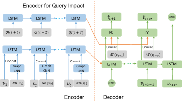
The hybrid model combines benefits from all available information domains. Figure 8 shows that the hybrid model enhances the Seq2Seq model with the attributes, the spatial relation, and the query impact. The spatial relation from $\bm{NB}(\bm{v}_{t})$ are incorporated into the encoder of the Seq2Seq model, while the attributes $\bm{AT}(\bm{v}_{t})$ and the query impact $\bm{QI(l,t)}$ are embedded into the decoder.

4. Experiments

In this section, we describe the compared methods, implementation details and evaluation metrics. We also discuss the results of different models.

4.1. Compared methods

We compare our proposed model with the following methods.

• Random forests (RF) (Leshem and Ritov, 2007): RF is a traditional machine learning method for regression, often used for traffic prediction;

• Support vector regression (SVR) (Jin et al., 2007): SVR is a version of SVM for regression, widely used in traffic prediction;

• Deep neural networks including the Seq2Seq model, the Seq2Seq + Attributes (AT) model, the Seq2Seq + Spatial relation (NB) model, the Seq2Seq + Query Impact (QI) model and the Hybrid Model that combines all three auxiliary domains.

Table 6. $Err_{T}$ (%): MAPE on the whole testing set. The results with the best performance are marked in bold.

Prediction	15-min	30-min	45-min	60-min	75-min	90-min	105-min	120-min	Overall
RF	6.00	9.15	10.20	10.66	10.98	11.21	11.39	11.56	10.14
SVR	5.44	9.20	10.07	10.34	10.51	10.65	10.76	10.83	9.73
Seq2Seq	4.61	8.22	9.28	9.72	9.98	10.27	10.48	10.61	9.23
Seq2Seq+AT	4.53	8.06	9.09	9.48	9.70	9.84	9.93	10.01	8.83
Seq2Seq+NB	4.52	8.05	9.07	9.45	9.67	9.83	9.93	9.99	8.81
Seq2Seq+QI	4.58	8.01	8.95	9.31	9.51	9.66	9.80	9.94	8.72
Hybrid	4.52	7.93	8.89	9.24	9.43	9.56	9.69	9.78	8.63

Table 7. $Err_{E}$ (%): MAPE during events on the testing set. The results with the best performance are marked in bold.

Prediction	15-min	30-min	45-min	60-min	75-min	90-min	105-min	120-min	Overall
RF	6.14	9.51	10.81	11.45	11.84	12.13	12.38	12.56	10.85
SVR	5.64	9.56	10.59	11.02	11.32	11.56	11.73	11.83	10.41
Seq2Seq	4.76	8.52	9.87	10.52	10.91	11.31	11.60	11.80	9.91
Seq2Seq+AT	4.65	8.32	9.63	10.23	10.58	10.81	10.98	11.13	9.54
Seq2Seq+NB	4.63	8.25	9.53	10.10	10.45	10.70	10.89	11.02	9.45
Seq2Seq+QI	4.69	8.18	9.37	9.93	10.28	10.55	10.77	10.98	9.34
Hybrid	4.61	8.09	9.30	9.84	10.16	10.39	10.60	10.76	9.22

4.2. Implementation Details

The traffic speed with 15-minute moving average is sampled at 15-minute intervals. One-day traffic speed sequence is used as inputs to predict future 2-hour traffic speed. Thus the length of the input sequence is $t=96$ and the length of the output sequence is $t^{\prime}=8$.

Given the traffic speed sequence $\{\bm{v}_{1},\bm{v}_{2},\dots,\bm{v}_{t}\}$, note that the standard Random Forests and SVR can only predict the traffic speed $\bm{v}_{t+1}$, whose goals are slightly different from our Seq2Seq model. So, on the testing stage, we treat prior forecasts as observations and use them for subsequent forecasts. For the Random Forests, the number of trees and the maximum depth are both 10. For SVR, we set $C=1,\epsilon=0.1$ and use RBF kernel. We use scikit-learn (Pedregosa et al., 2011) to implement the Random Forests and SVR.

All of the deep neural networks are implemented by TensorLayer (Dong et al., 2017) which is a deep learning and reinforcement learning library based on TensorFlow (Abadi et al., 2016). Stochastic gradient descent using the Adam optimiser (Kingma and Ba, 2014) is applied to update trainable parameters with mini-batch size 128. The deep neural networks are trained on a single NVIDIA GeForce GTX TITAN X GPU with 12GB memory.

The dimension of LSTM hidden state is set as 128. The social attributes have 6 dimensions and the geographical attributes have 131 dimensions. Half of the data (the first month) is used as the training set and the other half (the second month) is used for testing. The impact factor for calculating the query impact is $\sigma=150$.

4.3. Evaluation metrics

The mean absolute percentage error (MAPE) is used to evaluate the performance for comparisons, which is defined as

(8) $$MAPE = \frac{1}{T}\sum_{t=1}^{T}{\arrowvert\frac{\bm{v}_{t}-\tilde{\bm{v}}_{t}}{\bm{v}_{t}}\arrowvert}$$

where $\bm{v}_{t}$ and $\tilde{\bm{v}}_{t}$ are the actual and predicted traffic speed at time $t$, respectively. Two error rates are calculated. 1) $Err_{T}$ computes the MAPE across the whole testing set. 2) $Err_{E}$ only computes the MAPE during events on the testing set.

4.4. Results and discussion

Table 6 and Table 7 show quantitative comparison between different models. On the whole testing set, the hybrid model achieves the best performance with lowest overall MAPE 8.63% and 2-hour forecasting MAPE 9.78%. Compared with the common Seq2Seq model, auxiliary information (e.g., attributes, spatial relation and query impact) is able to improve the accuracy and the query impact is more effective than the other two domains.

It is more challenging to predict traffic when events happen, which is abnormally burst in traffic (Figure 1). Table 7 shows MAPE during events and the prediction is less accurate than that during normal conditions, especially for forecasting traffic more than one hour. With query impact, the hybrid model achieves the best performance with overall MAPE 9.22% and the Seq2Seq + Query Impact model achieves the second best accuracy with overall MAPE 9.34%.

Therefore, with appropriate integration of three kinds of auxiliary information, the deep encoder-decoder sequence networks can boost the traffic speed prediction during both events period and whole time period. Compared with the other two auxiliary domains, the query impact information has demonstrated larger improvement and promising application in the practical scenario.

5. Related Work

5.1. Traffic Prediction

Traffic prediction is a critical component in ITS. The methods of traffic prediction can be classified into parametric and non-parametric methods. Autoregressive integrated moving average (ARIMA) (Ahmed and Cook, 1979) is a widely used parametric technique for traffic prediction, which is based on the assumption that the traffic prediction is in a stationary process. However, ARIMA and its family require high computational resources and are not suitable for large-scale traffic data. Due to the stochastic and non-linear nature of traffic, researchers have paid much attention to the non-parametric methods, such as RF (Leshem and Ritov, 2007), SVR (Jin et al., 2007), online support vector regression (OL-SVR) (Castro-Neto et al., 2009), Bayesian network (Sun et al., 2006) and neural networks like ANN (Vlahogianni et al., 2005). Recently, some deep learning methods are proposed for traffic prediction such as stacked autoencoders (SAEs) (Lv et al., 2015), deep belief network (Huang et al., 2014). Most of them consider the traffic prediction for highways, whose traffic condition are relatively stable. However, in real-world cities, the traffic lights may have a great impact on the traffic speed, thus the traffic speed may vary greatly and previous methods may no longer work. (Ma et al., 2015) proposed to use long short-term memory network (LSTM) to predict traffic speed in cities. However, they only choose two points to conduct their experiments, which may be insufficient for practical applications.

5.2. Traffic Prediction via Auxiliary Domains

A few researchers have attempted to predict the traffic with related multimodal data. (He et al., 2013) (Liu et al., 2016) proposed an optimization framework to use traffic indicators extracted from social media with location information to model traffic sequence via linear regression. However, the traffic is a nonlinear system, so using a linear regression may be insufficient. (Ma et al., 2015) proposed an LSTM to forecast traffic speed given microwave detector data. However, in real-world road systems, only a small fraction of the road segments are deployed with sensors. For those road segments without sensors, previous methods may no longer work. Spatial dependencies among nodes can also improve traffic prediction (Asif et al., 2014) and (Yu et al., 2017; Ma et al., 2017) propose models based on CNN in order to incorporate spatial information.

6. Conclusions

As an important part of intelligent transportation systems, traffic prediction is limited by complex traffic environment in large cities and accessibility of high-quality multi-modal dataset. In this paper, we firstly introduce and release a large-scale traffic dataset, Q-Traffic, addressing the obstacle of the limited dataset. This dataset contains integrated online and offline auxiliary information including crowd map queries, road intersections and geographical and social attributes. Then we appropriately integrate traffic prediction with crowd map queries, road intersections and geographical and social attributes into a sequence to sequence learning framework, respectively. At last, a hybrid model is proposed to combine the benefits from all three auxiliary information domains and proved to be superior to compared methods, addressing the obstacles of traffic prediction with offline geographical factors and online potential influence. As for future work, with the release of the dataset, it is promising to attract more people to devise more approaches for accurate and real-time traffic prediction.