Majority vote model with ancillary noise in complex networks

Abstract

We analyze the properties of the majority-vote (MV) model with an additional noise in which a local spin can be changed independently of its neighborhood. In the standard MV, one of the simplest nonequilibrium systems exhibiting an order-disorder phase transition, spins are aligned with their local majority with probability $1-f$, and with complementary probability $f$, the majority rule is not followed. In the noisy MV (NMV), a random spin flip is succeeded with probability $p$ (with complementary $1-p$ the usual MV rule is accomplished). Such extra ingredient was considered by Vieira and Crokidakis [Physica A 450, 30 (2016)] for the square lattice. Here, we generalize the NMV for arbitrary networks, including homogeneous [random regular (RR) and Erdös Renyi (ER)] and heterogeneous [Barabasi-Albert (BA)] structures, through mean-field calculations and numerical simulations. Results coming from both approaches are in excellent agreement with each other, revealing that the presence of additional noise does not affect the classification of phase transition, which remains continuous irrespective of the network degree and its distribution. The critical point and the threshold probability $p_{t}$ marking the disappearance of the ordered phase depend on the node distribution and increase with the connectivity $k$. The critical behavior, investigated numerically, exhibits a common set of critical exponents for RR and ER topologies, but different from BA and regular lattices. Finally, our results indicate that (in contrary to a previous proposition) there is no first-order transition in the NMV for large $k$.

1 Introduction

Phase transitions and spontaneous breaking symmetry appear in a myriad of systems in the scope of physics [1, 2, 4, 5], biology [6], chemistry, social dynamics [7, 8] and others. Among the several microscopic models that exist in the literature, the Majority Vote (MV) model is probably one of the simplest nonequilibrium models exhibiting up-down $Z_{2}$ symmetry [4]. Its dynamics mimic the existence/formation of different opinions ($\pm 1$ in such case) in a community. In particular, it includes the role of individuals that do not adopt the local prevailing (majority) opinion, commonly referred to as contrarians or nonconformist characters. Therefore, it has attracted considerable attention recently, not only for theoretical purposes (including the investigation of critical behavior, universality classes, and phase coexistence) but also for the description (at least in a reduced level) of the mechanisms leading to the opinion formation [7, 8]. It is known that the phase transition exhibited by the MV model is continuous, signed by a spontaneous symmetry-breaking [4, 9, 10], although the critical behavior depends on lattice topology [4, 10].

An entirely different behavior was recently uncovered [11, 12] with the inclusion of a term proportional to the local spin (an inertial term), in which the phase transition becomes discontinuous. The effects of other ingredients, such as partial inertia [13], more states per site (instead of “up” or “down” as in the MV) [11, 14], and diffusion [15] have also been investigated.

The effect of an ancillary noise in the MV model was first studied by Vieira and Crokidakis [16]. In such noisy MV model (NMV), besides the intrinsic noise $f$, ruling the majority interaction to be or not to be accepted, one includes an independent term allowing a spin to be flipped irrespective of its neighborhood. In the social language jargon, this ingredient corresponds to another kind of nonconformism, usually referred to as independence. It was found a critical behavior in the square lattice identical to the that observed in the standard MV model, although the presence of extra noise provides an additional route for the emergence of the phase transition, even in the absence of misalignment term $f$ [16].

A relevant issue concerns in comparing the NMV with similar models in which the effect of independent noise has been undertaken. Recent studies for the $q$-voter model [5], in which a spin is flipped to the value of its $q$ nearest neighbors with a certain rate, reveal that the transition becomes discontinuous for large values of $q$, provided the independence ingredient is included. Due to the similarities between the $q-$voter model and the NMV, a natural question that arises is if that shift in the order of the phase transition is also verified in the NMV for high connectivity [16].

With these ideas in mind, here we analyze the NMV in distinct topologies for arbitrary connectivity. Through of mean-field calculations (MFT), we derive expressions for the critical points as a function of the extra noise for an arbitrary network topology. We employ a different (MFT) approach than Refs. [9, 17], which is based on an extension of the ideas from Ref. [4] for an arbitrary network structure. The critical behavior is also investigated by performing numerical simulations. Although MFT provides an approximate description of the phase transition, we observe an excellent agreement with numerical results in the regime of high connectivities. Our findings reveal the phase transition is continuous for all topologies and connectivities studied. Thus, contrasting to the $q-$voter model, a first-order transition is not observed in the NMV. Finally, our upshots also indicate the critical behavior in scale-free networks is different from that observed in homogeneous networks.

This paper is organized as follows: In Sec. II, we introduce the model and perform a mean field treatment. In Sec.III, we show and discuss our numerical results. At last, conclusions are drawn in Sec. IV.

2 Model and mean field analysis

The MV model is defined in an arbitrary lattice topology, in which each site $i$ of degree $k$ is attached to a binary spin variable, $\sigma_{i}$, that can take the values $\sigma_{i}=\pm 1$. In the original model, with probability $1-f$ each node $i$ tends to align itself with its local neighborhood majority, and with complementary probability $f$, the majority rule is not followed. The increase of the misalignment quantity $f$ gives rise to an order-disorder (continuous) phase transition [4, 10, 9]. The NMV differs from the original MV due to the inclusion of spin inversion independently of the neighborhood. Mathematically, it is equal to the following transition rate

$$w(\sigma_{i})=\frac{(1-p)}{2}[1-(1-2f)\sigma_{i}S(\sum_{j=1}^{k}\sigma_{j})]+\frac{p}{2},$$ (1)

where $S(X)$ is defined by $S(X)={\rm sign(X)}$ if $X\neq 0$ and $S(0)=0$. Note that for $p=0$ one recovers the original MV model. Since we are dealing with Markovian systems ruled by a master equation, our analysis starts by deriving the time evolution of the local magnetization of a site $i$ with degree $k$, $m_{k}=\langle\sigma_{i}\rangle_{k}$, given by $d\langle\sigma_{i}\rangle_{k}/dt=-\langle 2\sigma_{i}w(\sigma_{i})\rangle_{k}$. From the transition rate in Eq. (1), we have that

$$\frac{1}{1-p}\frac{d}{dt}m_{k}=-m_{k}+(1-2f)\langle S(X)\rangle-\frac{p}{1-p}m_{k}.$$ (2)

Our first inspection regarding the extra noise effect is carried out through a mean-field treatment. We shall consider a somewhat different approach (although equivalent) than Refs. [9, 17], in which the mean sign function is decomposed in two parts, $\langle S(X)\rangle=\langle S(X_{+})\rangle-\langle S(X_{-})\rangle$, with each term $\langle S(X_{i})\rangle$ being approximated as

$$\langle S\left(X_{\pm}\right)\rangle\approx\pm\sum_{n=\lceil k/2\rceil}^{k}C_{n}^{k}p_{\pm}^{n}p_{\mp}^{k-n}.$$ (3)

Here, each term $C_{n}^{k}$ in $\langle S\left(X_{\pm}\right)\rangle$ takes into account the number of possibilities of a neighborhood with $n$ and $k-n$ spins in the $+1(-1)$ and $-1(+1)$ states with associated probabilities $p_{+}(p_{-})$ and $p_{-}(p_{+})$, respectively. In the following, we shall relate $p_{\pm}$ to the local magnetization $m_{k}$. By focusing our analysis on uncorrelated structures, the probability $\rho_{k}$ of a local site presenting the spin $+1$ is related to $p_{\pm}$ through $p_{+}=\sum_{k}kP(k)\rho_{k}/\langle k\rangle$, where $P(k)$ is the degree probability distribution with mean value $\langle k\rangle$. Recalling that $\rho_{k}$ and $m_{k}$ are constrained through $m_{k}=2\rho_{k}-1$, the steady solution of Eq. (2) can be rewritten solely in terms of $p_{\pm}$ given by

$$p_{+}-\frac{1}{2}=\frac{(1-2f)}{2\langle k\rangle}\sum_{k=1}^{\infty}kP(k)\sum_{n=\lceil k/2\rceil}^{k}C_{n}^{k}(p_{+}^{n}p_{-}^{k-n}-p_{-}^{n}p_{+}^{k-n})-\frac{p}{1-p}(p_{+}-\frac{1}{2}).$$ (4)

It is possible to derive a simpler expression for $\langle S\left(X_{\pm}\right)\rangle$ for large $k$s, in which each term from the binomial distribution approaches to a Gaussian one with mean $kp_{\pm}$ and variance $\sigma^{2}=kp_{+}p_{-}$. So that $\sum_{n=\lceil k/2\rceil}^{k}C_{n}^{k}p_{\pm}^{n}p_{\mp}^{k-n}$ becomes $\int_{k/2}^{k}d\ell e^{-(\frac{\ell-kp_{\pm}}{\sqrt{2}\sigma})^{2}}/(\sigma\sqrt{2\pi})=\frac{\sqrt{\pi}}{2}({\rm erf}[\frac{k(1-p_{\pm})}{\sqrt{2}\sigma}]-{\rm erf}[\frac{k(1/2-p_{\pm})}{\sqrt{2}\sigma}])$, where ${\rm erf(x)}=2\int_{0}^{x}e^{-t^{2}}dt/\sqrt{\pi}$ denotes the error function. Thereby, the expression for the mean $\langle S(X)\rangle$ reads

$$\langle S(X)\rangle=\frac{1}{2}\left[2{\rm erf}\Bigg{(}\frac{\sqrt{2k}y}{\sqrt{1-4y^{2}}}\Bigg{)}+{\rm erf}\Bigg{(}\frac{\sqrt{2k}(\frac{1}{2}-y)}{\sqrt{1-4y^{2}}}\Bigg{)}-{\rm erf}\Bigg{(}\frac{\sqrt{2k}(\frac{1}{2}+y)}{\sqrt{1-4y^{2}}}\Bigg{)}\right],$$ (5)

where $p_{\pm}$ is rewritten in terms of the variable $y$ through the formula $p_{\pm}=\frac{1}{2}\pm y$ and for large $k$ Eq. (4) becomes

$$y=\frac{(1-2f)}{4\langle k\rangle}\sum_{k=1}^{\infty}kP(k)\left[2{\rm erf}\Bigg{(}\frac{\sqrt{2k}y}{\sqrt{1-4y^{2}}}\Bigg{)}+{\rm erf}\Bigg{(}\frac{\sqrt{2k}(\frac{1}{2}-y)}{\sqrt{1-4y^{2}}}\Bigg{)}-{\rm erf}\Bigg{(}\frac{\sqrt{2k}(\frac{1}{2}+y)}{\sqrt{1-4y^{2}}}\Bigg{)}\right]+$$

$$-\frac{p}{1-p}y.$$ (6)

Note that for large $k$ the numerator dominate over the denominator, so the second and third terms in the right side of Eqs. (5) and (6) cancel themselves and $\langle S(X)\rangle$ reduces to the simpler form $\langle S(X)\rangle={\rm erf}(y\sqrt{2k})$, from which we arrive at the following steady-state relation:

$$y=\frac{1}{2\langle k\rangle}(1-2f)\sum_{k}[k{\rm erf}(y\sqrt{2k})]P(k)-\frac{p}{1-p}y.$$ (7)

Thus, having the steady $y_{0}$s [from Eqs. (4) and (7)], the correspondent $m_{k}$ are then given by (for fixed $f$ and $p$)

$$m_{k}=(1-2f){\rm erf}(y\sqrt{2k})-\frac{p}{1-p}m_{k},$$ (8)

whose mean magnetization $m$ is finally evaluated through $m=\sum_{k=1}^{\infty}m_{k}P(k)$.

In order to derive a closed expression for the critical point, we should note that Eq. (7) presents two solutions ($y=\pm y_{0}\neq 0$) for $f<f_{c}$ (besides the trivial $y=0$) and only the trivial solution $y=0$ for $f>f_{c}$. Since $y_{0}$ is expected to be small close to the critical point, the first term in the right side of Eq. (7) can be expanded in Taylor series whose dependence on $f$ and $p$ (for arbitrary lattice topology) reads

$$y_{0}=\left\{\frac{1}{A(f,p)}\left[-1+(1-p)(1-2f)\sqrt{\frac{2}{\pi}}\frac{\langle k^{3/2}\rangle}{\langle k\rangle}\right]\right\}^{1/2},$$ (9)

where $\langle k^{3/2}\rangle=\sum_{k}k^{3/2}P(k)$ and $A(f,p)=\sqrt{\frac{8}{9\pi}}\frac{\langle k^{5/2}\rangle}{\langle k\rangle}(1-p)(1-2f)$. Finally, the critical $f_{c}$ is given by

$$f_{c}=\frac{1}{2}-\frac{1}{2}{\sqrt{\frac{\pi}{2}}}\frac{1}{1-p}\frac{\langle k\rangle}{\langle k^{3/2}\rangle},$$ (10)

with $A(p,f_{c})=2\langle k^{5/2}\rangle/\langle k^{3/2}\rangle$. In particular, for $p=0$ one recovers the expression $f_{c}=\frac{1}{2}-\frac{1}{2}{\sqrt{\frac{\pi}{2}}}\frac{\langle k\rangle}{\langle k^{3/2}\rangle}$, in consistency with the results from Ref. [9]. Complementary, an order-disorder phase transition is also obtained in the absence of misalignment $f=0$ by increasing the ancillary noise $p$, whose critical rate $p_{c}$ satisfies the relation $p_{c}=1-({\sqrt{\pi}}\langle k\rangle)/({\sqrt{2}}\langle k^{3/2}\rangle)$. Thus, above expression extends the conjecture $p_{c}(f=0)=2f_{c}(p=0)$, obtained for the square lattice [16], for arbitrary network distribution. A second MFT upshot to be drawn is that, contrasting to the generalized $q-$voter model [5], the inclusion of an independent noise does not alter the classification of phase transition, irrespective of the lattice topology and the neighborhood. The critical point, on the other hand, depends on the network topology.

The first structure we consider is a random regular network in which nodes follow the distribution $P(k)=\delta(k-k_{0})$, with $k_{0}$ being the degree. In this case, Eq. (10) becomes

$$f_{c}=\frac{1}{2}-\frac{1}{2}{\sqrt{\frac{\pi}{2k_{0}}}}\frac{1}{1-p}.$$ (11)

The second topology considered is the Erdös-Renyi (ER) network, an iconic example of a homogeneous random network, with a degree distribution given by $P(k)=\langle k\rangle^{k}e^{-\langle k\rangle}/k!$. Finally, a heterogeneous network, in which nodes are distributed according to a power-law distribution $P(k)\sim k^{-\gamma}$, is considered. For avoiding divergences when $k\rightarrow 0$ in the PL, we have imposed a minimum degree $k_{0}$ and the averages $\langle k\rangle$ and $\langle k^{3/2}\rangle$ become $\langle k\rangle=(\gamma-1)k_{0}/(\gamma-2)$ and $\langle k^{3/2}\rangle=(\gamma-1)k_{0}^{3/2}/(\gamma-5/2)$, respectively. Thus, the critical point $f_{c}$ reads

$$f_{c}=\frac{1}{2}-\frac{1}{2}{\sqrt{\frac{\pi}{2k_{0}}}}\frac{\gamma-5/2}{\gamma-2}\frac{1}{1-p}.$$ (12)

In this work, we shall focus on the analysis for $\gamma=3$, which is a hallmark of scale-free structures [19]. In the next section, we are going to confirm above findings by performing numerical simulations.

3 Numerical Results and phase diagrams

We have performed extensive numerical simulations for networks with sizes $N$ ranging from $N=1000$ to $20000$. We generated the RR networks through the classical configuration model, introduced by Bollobás [18]. The ER networks are constructed by connecting each pair of nodes with probability $\langle k\rangle/N$. When the size of the graph $N\rightarrow\infty$, the degree distribution is Poissonian, with mean $\langle k\rangle$. The Barabasi-Albert (BA) scale-free network is a typical representation of heterogeneous structures [19], in which the degree distribution follows a power-law $P(k)\sim k^{-\gamma}$ with scaling exponent $\gamma=3$.

Besides the order parameter vanishment, continuous phase transitions are signed by an algebraic divergence of the variance $\chi=N[\langle m^{2}\rangle-|m|^{2}]$ at the critical point $f_{c}$ for $N\rightarrow\infty$ [1, 2, 3]. Since only finite systems can be simulated, these quantities become rounded at the vicinity of criticality due to finite size effects. For calculating the critical point and the critical exponents, we resort to the finite size scaling theory, in which $|m|$ and $\chi$ are rewritten as $|m|=N^{-\beta/\nu}{\tilde{f}}(N^{1/\nu}|\epsilon|)$ and $\chi=N^{\gamma/\nu}{\tilde{g}}(N^{1/\nu}|\epsilon|)$, with ${\tilde{f}}$ and ${\tilde{g}}$ being scaling functions and $\epsilon=(f-f_{c})/f_{c}$. For $\epsilon=0$, the above relations acquire the dependence on the system size reading $|m|=N^{-\beta/\nu}{\tilde{f}}(0)$ and $\chi=N^{\gamma/\nu}{\tilde{g}}(0)$, in which a log-log plot of $|m|$ and $\chi$ versus $N$ furnish the exponents $\beta/\nu$ and $\gamma/\nu$, respectively.

Figure 1: Panels $(a)$ and $(b)$ show, for the RR networks and $p=0.1$ and $k_{0}=10$, the variance $\chi$ and the reduced cumulant $U_{4}$ versus $f$ for distinct system sizes $N$. Inset: the magnetization per spin $m$ vs. $f$. Panels $(c)$ and $(b)$ show the critical exponents $\beta/\nu$ and $\gamma/\nu$ for $p=0.1$ ($k_{0}=10$) and $p=0.5$($k_{0}=40$), respectively. They are consistent with $\beta/\nu=1/4$ and $\gamma/\nu=1/2$, respectively.

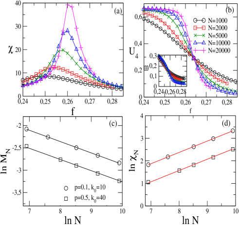
The critical point can be properly located through the reduced cumulant $U_{4}=1-\langle m^{4}\rangle/(3\langle m^{2}\rangle^{2})$, because curves for distinct $N$s cross at $f=f_{c}$ $(\epsilon=0)$ and $U_{4}$ becomes constant $U_{4}=U_{0}^{*}$. Off the critical point, $U_{4}\rightarrow 2/3$ and $0$ for the ordered and disordered phases, respectively when $N\rightarrow\infty$.

Figs. 1 and 2 exemplify the behavior of above quantities for the RR and ER cases for $p=0.1$ ($k_{0}=10$), $p=0.5$ ($k_{0}=40$) and $p=0.4$, $0.6$ ($\langle k\rangle=30$), respectively. Panels $(a)$ and $(b)$ reproduce the typical trademarks of critical transitions: $|m|$ decreases smoothly by raising $f$ (or $p$) and $\chi$ presents a maximum whose peak becomes more pronounced as $N$ increases. The nature of the phase transitions is reinforced by examining the crossing among the curves of $U_{4}$ for distinct system sizes. In all cases, the crossing is characterized by an apparent universal value $U_{0}^{*}=0.28(1)$.

Figure 2: Panels $(a)$ and $(b)$ show, for the ER case, $p=0.4$ and $\langle k\rangle=30$, the variance $\chi$ and the reduced cumulant $U_{4}$ versus $f$ for distinct system sizes $N$. Inset: Log-log plot of $y^{*}\equiv f_{c}-f_{N}$ versus $N$, with $f_{N}$ calculated from the maximum of $\chi$. The straight line has slope consistent to $1/\nu=1/2$. Panels $(c)$ and $(b)$ show the critical exponents $\beta/\nu$ and $\gamma/\nu$ for $p=0.4$ and $p=0.6$ (both for $\langle k\rangle=30$), respectively. They are consistent with $\beta/\nu=1/4$ and $\gamma/\nu=1/2$, respectively.

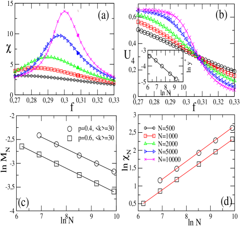
Analysis of the critical exponents furnish results consistent with $\beta/\nu=1/4$, $\gamma/\nu=1/2$ and $1/\nu=1/2$ (see inset of Fig. 2). Also, they satisfy the relation $2\beta/\nu+\gamma/\nu=D_{eff}$, with $D_{eff}=1$, indicating a universal behavior for homogeneous topologies. On the other hand, all of them are very different from the values $\beta=1/8$, $\gamma=7/4$ and $\nu=1$ for bidimensional (regular) lattices [16, 4].

Figure 3: Panels $(a)$ and $(b)$ show, for the BA network and $p=0.4$ and $k_{0}=20$, the variance $\chi$ and the reduced cumulant $U_{4}$ versus $f$ for distinct system sizes $N$. Panels $(c)$ and $(b)$ show the critical exponents $\beta/\nu$ and $\gamma/\nu$ for $p=0.4$ ($k_{0}=20$) and $p=0.6$ ($k_{0}=10$), respectively. They are consistent with $\beta/\nu=0.34(1)$ and $\gamma/\nu=0.32(1)$, respectively.

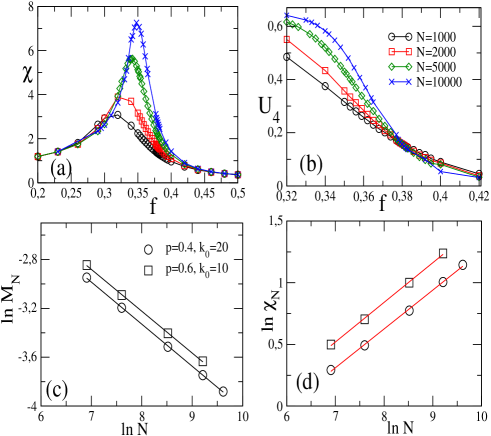
A slightly distinct critical behavior is obtained for the BA network, exemplified in Fig. 3 for $p=0.4$ ($k_{0}=20$) and $p=0.6$ ($k_{0}=10$). In both cases, the crossing value $U_{0}^{*}$ and the set of critical exponents are other than those obtained for the homogeneous structures, reading $U_{0}^{*}=0.16(1)$ and critical exponents $\beta/\nu=0.34(1)$ and $\gamma/\nu=0.32(1)$, respectively. Albeit, they also fulfill the relation $2\beta/\nu+\gamma/\nu=1$.

Figure 4: Panel $(a)$ shows, for the RR network, the transition rates $f_{c}$ versus the degree node $k_{0}$ for distinct values of $p$. Circles and lines correspond to the estimates obtained from Eqs. (4) and (11), respectively. The symbol $\times$ correspond to the numerical values obtained from the crossing among $U_{4}$ for distinct $N$s. Panel $(b)$ shows the phase diagram $p_{c}$ versus $f_{c}$ for distinct $k_{0}$s.

Figure 5: Panel $(a)$ shows, for the ER case, the transition rates $f_{c}$ versus the mean degree $\langle k\rangle$ for distinct values of $p$. Circles and lines correspond to estimates obtained from Eqs. (4) and (10), respectively. The symbol $\times$ correspond to the numerical values obtained from the crossing among $U_{4}$ for distinct $N$s. Panel $(b)$ shows the phase diagram $p_{c}$ versus $f_{c}$ for distinct $\langle k\rangle$s.

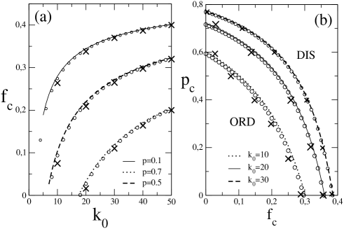
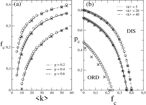
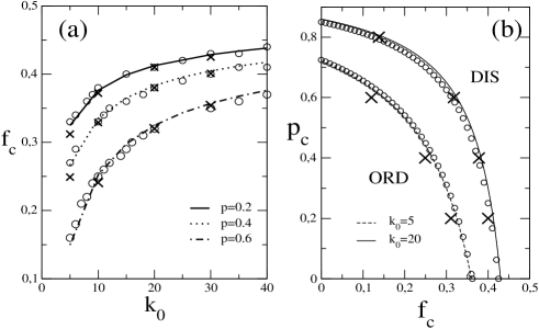
Now let us examine the phase diagrams. A comparison of the results for distinct topologies is shown in Figs. 4-6 for distinct values of $p$, $k_{0}$ (RR and BA) and $\langle k\rangle$ (ER). Panels $(a)$ show that all estimates agree very well for high connectivities, but some discrepancies arise for the systems with lower degrees. These trends reveal not only the reliability of one-site MFT but also its accuracy for the location of the critical point. As in the MFT, the phase transitions are continuous, irrespective of the lattice topology and the system degree. This result, contrasts to the observed in the $q-$voter model, where the inclusion of “independence” does turn the phase transition into a discontinuous one [5]. According to [5], whenever the “anti-conformism rule” is drawn, the chosen site (always) flips its spin provided all its $q$ neighbors have opposite spins. This interaction rule is slightly different from the usual majority one, in which the spin flip depends only on the signal of the spin neighborhood and always there is a finite probability of the majority rule not to be followed (except to $f=0$). Also, increasing the ancillary $p$ does not alter the discrepancies among these methods. Finally, we observe that [panels $(b)$] the inclusion of additional noise shortens the ordered phase and thus the disordered region enlarges.

Figure 6: Panel $(a)$ shows, for the BA case, the transition rates $f_{c}$ versus the minimum degree $k_{0}$ for distinct values of $p$. Circles and lines correspond to estimates obtained from Eqs. (4) and (12), respectively. The symbol $\times$ correspond to the numerical values obtained from the crossing among fourth-order reduced cumulant for distinct network sizes. Panel $(b)$ shows the phase diagram $p_{c}$ versus $f_{c}$ for distinct $k_{0}$s.

4 Conclusions

We have investigated the majority vote model in complex networks, in the presence of two distinct kinds of noise. Our study, through numerical simulations and mean-field theory, considered both homogeneous and heterogeneous (scale-free) topologies. We have derived expressions (through a different mean-field approach than Refs. [17, 9]) for the critical point in terms of the network topology and the noise parameter $p$. The resulting expressions work very well in the regime of high connectivity. The critical behavior and the set of critical exponents have been investigated in detail. Our numerical results strongly suggest the existence of a common set of critical exponents for the random regular and Erdös-Renyi networks. On the other hand, they are different for heterogeneous structures, suggesting a novel universality class for the MV in scale-free structures. Due to the scarcity of results [20], we believe that our findings constitute an important step for classifying the critical behavior in scale-free networks. However, we remark that further studies are still required to a complete classification. In particular, a comparison between the critical behavior exhibited in other heterogeneous structures, such as the uncorrelated configuration model (UCM) [21], can be very interesting. Finally, the previous proposal of a discontinuous phase transition in the regime of high connectivity (irrespective of the network topology) is discarded [16].

5 Acknowledgement

We acknowledge the financial support from CNPq, FAPESP under grant 2018/02405-1.

References

- [1] J. Marro and R. Dickman, Nonequilibrium Phase Transitions in Lattice Models (Cambridge University Press, Cambridge, 1999).
- [2] G. Ódor, Universality In Nonequilibrium Lattice Systems: Theoretical Foundations (World Scientific,Singapore, 2007).
- [3] M. Henkel, H. Hinrichsen and S. Lubeck, Non-Equilibrium Phase Transitions Volume I: Absorbing Phase Transitions (Springer-Verlag, The Netherlands, 2008).
- [4] M. J. de Oliveira, J. Stat. Phys. 66, 273 (1992).
- [5] P. Nyczka, K. Sznajd-Weron and J. Cislo, Phys. Rev. E, 86, 011105 (2012).
- [6] T. Vicsek and A. Zafeiris, Physics Reports 517, 71 (2012).
- [7] C. Castellano, S. Fortunato, and V. Loreto, Rev. Mod. Phys. 81, 591 (2009).
- [8] C. Castellano, M. Marsili, and A. Vespignani, Phys. Rev. Lett. 85, 3536 (2000).
- [9] H. Chen, C. Shen, G. He, H. Zhang and Z. Hou, Phys, Rev. E 91, 022816 (2015).
- [10] L. F. C. Pereira and F. G. B. Moreira, Phys. Rev. E 71, 016123 (2005).
- [11] H. Chen, C. Shen, H. Zhang, G. Li, Z. Hou and J. Kurths, Phys Rev. E 95, 042304 (2017).
- [12] J. M. Encinas, P. E. Harunari, M. M. de Oliveira and C. E. Fiore, Sci. Rep. 8, 9338 (2018) .
- [13] P. E. Harunari, M. M. de Oliveira and C. E. Fiore, Phys. Rev. E 96, 042305 (2017).
- [14] D. F. F. Melo, L. F. Pereira and F. G. B. Moreira, J. Stat. Mech. P11032 (2010); F. W. S. Lima, Physica A 391, 1752 (2012)
- [15] N. Crokidakis and P. M. C. de Oliveira, Phys. Rev. E 85, 041147 (2012).
- [16] A. R. Vieira and N. Crokidakis, Physica A 450, 30 (2016).
- [17] C. Castellano and R. Pastor-Satorras, J. Stat. Mech. p. P05001 (2006).
- [18] B. Bollobás, Europ. J. Combinatorics. 1, 311 (1980).
- [19] A.-L. Barabási and R. Albert, Science 286, 509 (1999).
- [20] F. W. S. Lima, Int. J. Mod. Phys. C, 17, 1257 (2006).
- [21] M. Catanzaro, M. Boguna and R. Pastor-Satorras, Phys. Rev. E 71, 027103 (2005).