Statistical Optimal Transport via Factored Couplings

Abstract

We propose a new method to estimate Wasserstein distances and optimal transport plans between two probability distributions from samples in high dimension. Unlike plug-in rules that simply replace the true distributions by their empirical counterparts, our method promotes couplings with low transport rank, a new structural assumption that is similar to the nonnegative rank of a matrix. Regularizing based on this assumption leads to drastic improvements on high-dimensional data for various tasks, including domain adaptation in single-cell RNA sequencing data. These findings are supported by a theoretical analysis that indicates that the transport rank is key in overcoming the curse of dimensionality inherent to data-driven optimal transport.

tprP.R. is supported in part by NSF grants DMS-1712596 and TRIPODS-1740751 and IIS-1838071, ONR grant N00014-17-1-2147, the Chan Zuckerberg Initiative DAF 2018-182642, and the MIT Skoltech Seed Fund. tmnM.N. is supported by the James S. McDonnell Foundation, Schmidt Futures, Israel Council for Higher Education, and the John Harvard Distinguished Science Fellows Program. tjwJ.W. is supported in part by the Josephine de Karman fellowship. tgwG.S. is supported by a Career Award at the Scientific Interface from the Burroughs Welcome Fund and by the Klarman Cell Observatory.

1 INTRODUCTION

Optimal transport (OT) was born from a simple question phrased by Gaspard Monge in the eighteenth century [Monge, 1781] and has since flourished into a rich mathematical theory two centuries later [Villani, 2003, 2009]. Recently, OT and more specifically Wasserstein distances, which include the so-called earth mover’s distance [Rubner et al., 2000] as a special example, have proven valuable for varied tasks in machine learning [Bassetti et al., 2006, Cuturi, 2013, Cuturi and Doucet, 2014b, Solomon et al., 2014b, Frogner et al., 2015, Srivastava et al., 2015, Genevay et al., 2016, Gao and Kleywegt, 2016, Rolet et al., 2016, Genevay et al., 2017, Rigollet and Weed, 2018a, b], computer graphics [Bonneel et al., 2011, de Goes et al., 2012, Solomon et al., 2014a, 2015, Bonneel et al., 2016], geometric processing [de Goes et al., 2011, Solomon et al., 2013], image processing [Gramfort et al., 2015, Rabin and Papadakis, 2015], and document retrieval [Ma et al., 2014, Kusner et al., 2015]. These recent developments have been supported by breakneck advances in computational optimal transport in the last few years that allow the approximation of these distances in near linear time [Cuturi, 2013, Altschuler et al., 2017].

In these examples, Wasserstein distances and transport plans are estimated from data. Yet, the understanding of statistical aspects of OT is still in its infancy. In particular, current methodological advances focus on computational benefits but often overlook statistical regularization to address stability in the presence of sampling noise. Known theoretical results show that vanilla optimal transport applied to sampled data suffers from the curse of dimensionality [Dudley, 1969, Dobrić and Yukich, 1995, Weed and Bach, 2017] and the need for principled regularization techniques is acute in order to scale optimal transport to high-dimensional problems, such as those arising in genomics, for example.

At the heart of OT is the computation of Wasserstein distances, which consists of an optimization problem over the infinite dimensional set of couplings between probability distributions. (See (1) for a formal definition.) Estimation in this context is therefore nonparametric in nature and this is precisely the source of the curse of dimensionality. To overcome this limitation, and following a major trend in high-dimensional statistics [Candès and Plan, 2010, Liu et al., 2010, Markovsky and Usevich, 2012], we propose to impose low “rank” structure on the couplings. Interestingly, this technique can be implemented efficiently via Wasserstein barycenters [Agueh and Carlier, 2011, Cuturi and Doucet, 2014a] with finite support.

We illustrate the performance of this new procedure for a truly high-dimensional problem arising in single-cell RNA sequencing data, where ad-hoc methods for domain adaptation have recently been proposed to couple datasets collected in different labs and with different protocols [Haghverdi et al., 2017], and even across species [Butler et al., 2018]. Despite a relatively successful application of OT-based methods in this context [Schiebinger et al., 2017], the very high-dimensional and noisy nature of this data calls for robust statistical methods. We show in this paper that our proposed method does lead to improved results for this application.

This paper is organized as follows. We begin by reviewing optimal transport in §2, and we provide an overview of our results in §3. Next, we introduce our estimator in §4. This is a new estimator for the Wasserstein distance between two probability measures that is statistically more stable than the naive plug-in estimator that has traditionally been used. This stability guarantee is not only backed by the theoretical results of §5, but also observed in numerical experiments in practice §6.

Notation. We denote by $\|\cdot\|$ the Euclidean norm over ${\rm I}\kern-1.79993pt{\rm R}^{d}$. For any $x\in{\rm I}\kern-1.79993pt{\rm R}^{d}$, let $\delta_{x}$ denote the Dirac measure centered at $x$. For any two real numbers $a$ and $b$, we denote their minimum by $a\wedge b$. For any two sequences $u_{n},v_{n}$, we write $u_{n}\lesssim v_{n}$ when there exists a constant $C>0$ such that $u_{n}\leq Cv_{n}$ for all $n$. If $u_{n}\lesssim v_{n}$ and $v_{n}\lesssim u_{n}$, we write $u_{n}\asymp v_{n}$. We denote by $\mathbf{1}_{n}$ the all-ones vector of ${\rm I}\kern-1.79993pt{\rm R}^{n}$, and by $e_{i}$ the $i$th standard vector in ${\rm I}\kern-1.79993pt{\rm R}^{n}$. Moreover, we denote by $\odot$ and $\oslash$ element-wise multiplication and division of vectors, respectively.

For any map $f:{\rm I}\kern-1.79993pt{\rm R}^{d}\to{\rm I}\kern-1.79993pt{\rm R}^{d}$ and measure $\mu$ on ${\rm I}\kern-1.79993pt{\rm R}^{d}$, let $f_{\#}\mu$ denote the pushforward measure of $\mu$ through $f$ defined for any Borel set $A$ by $f_{\#}\mu(A)=\mu\big{(}f^{-1}(A)\big{)}$, where $f^{-1}(A)=\{x\in{\rm I}\kern-1.79993pt{\rm R}^{d}\,:f(x)\in A\}$. Given a measure $\mu$, we denote its support by $\mathrm{supp}(\mu)$.

2 BACKGROUND ON OPTIMAL TRANSPORT

In this section, we gather the necessary background on optimal transport. We refer the reader to recent books [Santambrogio, 2015, Villani, 2003, 2009] for more details.

Wasserstein distance

Given two probability measures $P_{0}$ and $P_{1}$ on ${\rm I}\kern-1.79993pt{\rm R}^{d}$, let $\Gamma(P_{0},P_{1})$ denote the set of couplings between $P_{0}$ and $P_{1}$, that is, the set of joint distributions with marginals $P_{0}$ and $P_{1}$ respectively so that $\gamma\in\Gamma(P_{0},P_{1})$ iff $\gamma(U\times{\rm I}\kern-1.79993pt{\rm R}^{d})=P_{0}(U)$ and $\gamma({\rm I}\kern-1.79993pt{\rm R}^{d}\times V)=P_{1}(V)$ for all measurable $U,V\in{\rm I}\kern-1.79993pt{\rm R}^{d}$.

The $2$-Wasserstein distance between two probability measures $P_{0}$ and $P_{1}$ is defined as

$$W_{2}(P_{0},P_{1}):=\inf_{\gamma\in\Gamma(P_{0},P_{1})}\sqrt{\int_{{\rm I}\kern-1.25995pt{\rm R}^{d}\times{\rm I}\kern-1.25995pt{\rm R}^{d}}\|x-y\|^{2}\,\mathrm{d}\gamma(x,y)}\,.$$ (1)

Under regularity conditions, for example if both $P_{0}$ and $P_{1}$ are absolutely continuous with respect to the Lebesgue measure, it can be shown the infimum in (1) is attained at a unique coupling $\gamma^{*}$. Moreover $\gamma^{*}$ is a deterministic coupling: it is supported on a set of the form $\{(x,T(x))\,:\,x\in\mathrm{supp}(P_{0})\}$. In this case, we call $T$ a transport map. In general, however, $\gamma^{*}$ is unique but for any $x_{0}\in\mathrm{supp}(P_{0})$, the support of $\gamma^{*}(x_{0},\cdot)$ may not reduce to a single point, in which case, the map $x\mapsto\gamma^{*}(x,\cdot)$ is called a transport plan.

Wasserstein space

The space of probability measures with finite $2$nd moment equipped with the metric $W_{2}$ is called Wasserstein space and denoted by $\mathcal{W}_{2}$. It can be shown that $\mathcal{W}_{2}$ is a geodesic space: given two probability measures $P_{0},P_{1}\in\mathcal{W}_{2}$, the constant speed geodesic connecting $P_{0}$ and $P_{1}$ is the curve $\{P_{t}\}_{t\in[0,1]}$ defined as follows. Let $\gamma^{*}$ be the optimal coupling defined as the solution of (1), and for $t\in[0,1]$ let $\pi_{t}:{\rm I}\kern-1.79993pt{\rm R}^{d}\times{\rm I}\kern-1.79993pt{\rm R}^{d}\to{\rm I}\kern-1.79993pt{\rm R}$ be defined as $\pi_{t}(x,y)=(1-t)x+ty$, then $P_{t}=(\pi_{t})_{\#}\gamma^{*}$. We then call $P_{1/2}$ the geodesic midpoint of $P_{0}$ and $P_{1}$. It plays the role of an average in Wasserstein space, which, unlike the mixture $(P_{0}+P_{1})/2$, takes the geometry of ${\rm I}\kern-1.79993pt{\rm R}^{d}$ into account.

$k$-Wasserstein barycenters

The now-popular notion of Wasserstein barycenters (WB) was introduced by Agueh and Carlier [2011] as a generalization of the geodesic midpoint $P_{1/2}$ to more than two measures. In its original form, a WB can be any probability measure on ${\rm I}\kern-1.79993pt{\rm R}^{d}$, but algorithmic considerations led Cuturi and Doucet [Cuturi and Doucet, 2014a] to restrict the support of a WB to a finite set of size $k$. Let $\mathcal{D}_{k}$ denote the set of probability distributions supported on $k$ points:

$$\mathcal{D}_{k}=\left\{\sum_{j=1}^{k}\alpha_{j}\delta_{x_{j}}\,:\,\alpha_{j}\geq 0,\sum_{j=1}^{k}\alpha_{j}=1,x_{j}\in{\rm I}\kern-1.79993pt{\rm R}^{d}\right\}.$$

For a given integer $k$, the $k$-Wasserstein Barycenter $\bar{P}$ between $N$ probability measures $P_{0},\ldots P_{N}$ on ${\rm I}\kern-1.79993pt{\rm R}^{d}$ is defined by

$$\bar{P}=\mathop{\mathrm{argmin}}_{P\in\mathcal{D}_{k}}\sum_{j=1}^{N}W_{2}^{2}(P,P^{(j)})\,.$$ (2)

In general (2) is not a convex problem but fast numerical heuristics have demonstrated good performance in practice [Cuturi and Doucet, 2014a, Cuturi and Peyré, 2016, Benamou et al., 2015, Staib et al., 2017, Claici et al., 2018]. Interestingly, Theorem 4 below indicates that the extra constraint $P\in\mathcal{D}_{k}$ is also key to statistical stability.

3 RESULTS OVERVIEW

Ultimately, in all the data-driven applications cited above, Wasserstein distances must be estimated from data. While this is arguably the most fundamental primitive of all OT based machine learning, the statistical aspects of this question are often overlooked at the expense of computational ones. We argue that standard estimators of both $W_{2}(P_{0},P_{1})$ and its associated optimal transport plan suffer from statistical instability. The main contribution of this paper is to overcome this limitation by injecting statistical regularization.

Previous work

Let $X\sim P_{0}$ and $Y\sim P_{1}$ and let $X_{1},\ldots,X_{n}$ (resp. $Y_{1},\ldots,Y_{n}$) be independent copies of $X$ (resp. $Y$). We call $\mathcal{X}=\{X_{1},\ldots,X_{n}\}$ and $\mathcal{Y}=(Y_{1},\ldots,Y_{n})$ the source and target datasets respectively. Define the corresponding empirical measures:

$$\hat{P}_{0}=\frac{1}{n}\sum_{i=1}^{n}\delta_{X_{i}}\,,\qquad\hat{P}_{1}=\frac{1}{n}\sum_{i=1}^{n}\delta_{Y_{i}}\,.$$ (3)

Perhaps the most natural estimator for $W_{2}(P_{0},P_{1})$, and certainly the one most employed and studied, is the plug-in estimator $W_{2}(\hat{P}_{0},\hat{P}_{1})$. A natural question is to determine the accuracy of this estimator. This question was partially addressed by Sommerfeld and Munk [Sommerfeld and Munk, 2017], where the rate at which $\Delta_{n}:=|W_{2}(\hat{P}_{0},\hat{P}_{1})-W_{2}(P_{0},P_{1})|$ vanishes is established. They show that $\Delta_{n}\asymp n^{-1/2}$ if $P_{0}\neq P_{1}$ and $\Delta_{n}\asymp n^{-1/4}$ if $P_{0}=P_{1}$. Unfortunately, these rates are only valid when $P_{0}$ and $P_{1}$ have finite support. Moreover, the plug-in estimator for distributions ${\rm I}\kern-1.79993pt{\rm R}^{d}$ has been known to suffer from the curse of dimensionality at least since the work of Dudley [Dudley, 1969]. More specifically, in this case, $\Delta_{n}\asymp n^{-1/d}$ when $d\geq 3$ [Dobrić and Yukich, 1995]. One of the main goals of this paper is to provide an alternative to the naive plug-in estimator by regularizing the optimal transport problem (1). Explicit regularization for optimal transport problems was previously introduced by Cuturi [Cuturi, 2013] who adds an entropic penalty to the objective in (1) primarily driven by algorithmic motivations. While entropic OT was recently shown [Rigollet and Weed, 2018b] to also provide statistical regularization, that result indicates that entropic OT does not alleviate the curse of dimensionality coming from sampling noise, but rather addresses the presence of additional measurement noise.

Closer to our setup are Courty et al. [2014] and Ferradans et al. [2014]; both consider sparsity-inducing structural penalties that are relevant for domain adaptation and computer graphics, respectively. While the general framework of Tikhonov-type regularization for optimal transport problems is likely to bear fruit in specific applications, we propose a new general-purpose structural regularization method, based on a new notion of complexity for joint probability measures.

Our contribution

The core contribution of this paper is to construct an estimator of the Wasserstein distance between distributions that is more stable and accurate under sampling noise. We do so by defining a new regularizer for couplings, which we call the transport rank. As a byproduct, our estimator also yields an estimator of the optimal coupling in (1) that can in turn be used in domain adaptation where optimal transport has recently been employed [Courty et al., 2014, 2017].

To achieve this goal, we leverage insights from a popular technique known as nonnegative matrix factorization (NMF) [Paatero and Tapper, 1994, Lee and Seung, 2001] which has been successfully applied in various forms to many fields, including text analysis [Shahnaz et al., 2006], computer vision [Shashua and Hazan, 2005], and bioinformatics [Gao and Church, 2005]. Like its cousin factor analysis, it postulates the existence of low-dimensional latent variables that govern the high-dimensional data-generating process under study.

In the context of optimal transport, we consider couplings $\gamma\in\Gamma(P_{0},P_{1})$ such that whenever $(X,Y)\sim\gamma$, there exits a latent variable $Z$ with finite support such that $X$ and $Y$ are conditionally independent given $Z$. To see the analogy with NMF, one may view a coupling $\gamma$ as a doubly stochastic matrix whose rows and columns are indexed by ${\rm I}\kern-1.79993pt{\rm R}^{d}$. We consider couplings such that this matrix can be written as the product $AB$ where $A$ and $B^{\top}$ are matrices whose rows are indexed by ${\rm I}\kern-1.79993pt{\rm R}^{d}$ and columns are indexed by $\{1,\ldots k\}$. In that case, we call $k$ the transport rank of $\gamma$. We now formally define these notions.

Definition 1.

Given $\gamma\in\Gamma(P_{0},P_{1})$, the transport rank of $\gamma$ is the smallest integer $k$ such that $\gamma$ can be written

$$\gamma=\sum_{j=1}^{k}\lambda_{j}(Q^{0}_{j}\otimes Q^{1}_{j})\,,$$ (4)

where the $Q^{0}_{j}$’s and $Q^{1}_{j}$’s are probability measures on ${\rm I}\kern-1.79993pt{\rm R}^{d}$, $\lambda_{j}\geq 0$ for $j=1,\dots,k$, and where $Q^{0}_{j}\otimes Q^{1}_{j}$ indicates the (independent) product distribution. We denote the set of couplings between $P_{0}$ and $P_{1}$ with transport rank at most $k$ by $\Gamma_{k}(P_{0},P_{1})$.

When $P_{0}$ and $P_{1}$ are finitely supported, the transport rank of $\gamma\in\Gamma(P_{0},P_{1})$ coincides with the nonnegative rank [Yannakakis, 1991, Cohen and Rothblum, 1993] of $\gamma$ viewed as a matrix. By analogy with a nonnegative factorization of a matrix, we call a coupling written as a sum as in (4) a factored coupling. Using the transport rank as a regularizer therefore promotes simple couplings, i.e., those possessing a low-rank “factorization.” To implement this regularization, we show that it can be constructed via $k$-Wasserstein barycenters, for which efficient implementation is readily available.

As an example of our technique, we show in §6 that this approach can be used to obtain better results on domain adaptation a.k.a transductive learning, a strategy in semi-supervised learning to transfer label information from a source dataset to a target dataset. Notably, while regularized optimal transport has proved to be an effective tool for supervised domain adaptation where label information is used to build an explicit Tikhonov regularization [Courty et al., 2014], our approach is entirely unsupervised, in the spirit of Gong et al. [2012] where unlabeled datasets are matched and then labels are transported from the source to the target. We argue that both approaches, supervised and unsupervised, have their own merits but the unsupervised approach is more versatile and calibrated with our biological inquiry regarding single cell data integration.

4 REGULARIZATION VIA FACTORED COUPLINGS

To estimate the Wasserstein distance between $P_{0}$ and $P_{1}$, we find a low-rank factored coupling between the empirical distributions. As we show in §5, the bias induced by this regularizer provides significant statistical benefits. Our procedure is based on an intuitive principle: optimal couplings arising in practice can be well approximated by assuming the distributions have a small number of pieces moving nearly independently. For example, if distributions represent populations of cells, this assumption amounts to assuming that there are a small number of cell “types,” each subject to different forces.

Before introducing our estimator, we note that a factored coupling induces coupled partitions of the source and target distributions. These clusterings are “soft” in the sense that they may include fractional points.

Definition 2.

Given $\lambda\in[0,1]$, a soft cluster of a probability measure $P$ is a sub-probability measure $C$ of total mass $\lambda$ such that $0\leq C\leq P$ as measures. The centroid of $C$ is defined by $\mu(C)=\frac{1}{\lambda}\int x\,\mathrm{d}C(x)$. We say that a collection $C_{1},\dots,C_{k}$ of soft clusters of $P$ is a partition of $P$ if $C_{1}+\dots+C_{k}=P$.

The following fact is immediate.

Proposition 4.1.

If $\gamma=\sum_{j=1}^{k}\lambda_{j}(Q^{0}_{j}\otimes Q^{1}_{j})$ is a factored coupling in $\Gamma_{k}(P_{0},P_{1})$, then $\{\lambda_{1}Q^{0}_{1},\dots,\lambda_{k}Q^{0}_{k}\}$ and $\{\lambda_{1}Q^{1}_{1},\dots,\lambda_{k}Q^{1}_{k}\}$ are partitions of $P_{0}$ and $P_{1}$, respectively.

We now give a simple characterization of the “cost” of a factored coupling.

Proposition 4.2.

Let $\gamma\in\Gamma_{k}(P_{0},P_{1})$ and let $C_{1}^{0},\dots,C_{k}^{0}$ and $C_{1}^{1},\dots,C_{k}^{1}$ be the induced partitions of $P_{0}$ and $P_{1}$, with $C_{j}^{0}({\rm I}\kern-1.79993pt{\rm R}^{d})=C_{j}^{1}({\rm I}\kern-1.79993pt{\rm R}^{d})=\lambda_{j}$ for $j=1,\dots k$. Then

$$\int\|x-y\|^{2}\,\mathrm{d} \gamma(x,y)=\sum_{j=1}^{k}\Big{(}\lambda_{j}\|\mu(C_{j}^{0})-\mu(C_{j}^{1})\|^{2}$$

$$+\sum_{l\in\{0,1\}}\int\|x-\mu(C_{j}^{l})\|^{2}\,\mathrm{d}C_{j}^{l}(x)\Big{)}$$

The sum over $l$ in the above display contains intra-cluster variance terms similar to the $k$-means objective, while the first term is a transport term reflecting the cost of transporting the partition of $P_{0}$ to the partition of $P_{1}$. Since our goal is to estimate the transport distance, we focus on the first term. This motivates the following definition.

Definition 3.

The cost of a factored transport $\gamma\in\Gamma_{k}(P_{0},P_{1})$ is

$$\operatorname{cost}(\gamma):=\sum_{j=1}^{k}\lambda_{j}\|\mu(C_{j}^{0})-\mu(C_{j}^{1})\|^{2}\,$$

where $\{C_{j}^{0}\}_{j=1}^{k}$ and $\{C_{j}^{1}\}_{j=1}^{k}$ are the partitions of $P_{0}$ and $P_{1}$ induced by $\gamma$, with $C_{j}^{0}({\rm I}\kern-1.79993pt{\rm R}^{d})=C_{j}^{1}({\rm I}\kern-1.79993pt{\rm R}^{d})=\lambda_{j}$ for $j=1,\dots,k$.

Given empirical distributions $\hat{P}_{0}$ and $\hat{P}_{1}$, the (unregularized) optimal coupling between $\hat{P}_{0}$ and $\hat{P}_{1}$, defined as

$$\mathop{\mathrm{argmin}}_{\gamma\in\Gamma(\hat{P}_{0},\hat{P}_{1})}\int\|x-y\|^{2}\mathrm{d}\gamma(x,y)\,,$$

is highly non-robust with respect to sampling noise. This motivates considering instead the regularized version

$$\mathop{\mathrm{argmin}}_{\gamma\in\Gamma_{k}(\hat{P}_{0},\hat{P}_{1})}\int\|x-y\|^{2}\mathrm{d}\gamma(x,y)\,,$$ (5)

where $k\geq 1$ is a regularization parameter. Whereas fast solvers are available for the unregularized problem [Altschuler et al., 2017], it is not clear how to find a solution to (5) by similar means. While alternating minimization approaches similar to heuristics for nonnegative matrix factorization are possible [Lee and Seung, 2001, Arora et al., 2012], we adopt a different approach which has the virtue of connecting (5) to $k$-Wasserstein barycenters.

Following Cuturi and Doucet [2014a], define the $k$-Wasserstein barycenter of $\hat{P}_{0}$ and $\hat{P}_{1}$ by

$$H=\mathop{\mathrm{argmin}}_{P\in\mathcal{D}_{k}}\,\,\left\{W_{2}^{2}(P,\hat{P}_{0})+W_{2}^{2}(P,\hat{P}_{1})\right\}\,.$$ (6)

As noted above, while this objective is not convex, efficient procedures have been shown to work well in practice.

Strikingly, the $k$-Wasserstein barycenter of $\hat{P}_{0}$ and $\hat{P}_{1}$ implements a slight variant of (5). Given a feasible $P\in\mathcal{D}_{k}$ in (6), we first note that it induces a factored coupling in $\Gamma_{k}(\hat{P}_{0},\hat{P}_{1})$. Indeed, denote by $\gamma_{0}$ and $\gamma_{1}$ the optimal couplings between $\hat{P}_{0}$ and $P$ and $P$ and $\hat{P}_{1}$, respectively. Write $z_{1},\dots,z_{j}$ for the support of $P$. We can then decompose these couplings as follows:

$$\gamma_{0}=\sum_{j=1}^{k}\gamma_{0}(\cdot\mid z_{j})H(z_{j}),\quad\gamma_{1}=\sum_{j=1}^{k}\gamma_{1}(\cdot\mid z_{j})H(z_{j})$$

Then for any Borel sets $A,B\subset{\rm I}\kern-1.79993pt{\rm R}^{d}$,

$$\gamma_{P}(A\times B):=\sum_{j=1}^{k}P(z_{j})\gamma_{0}(A|z_{j})\gamma_{1}(B|z_{j})\in\Gamma_{k}(\hat{P}_{0},\hat{P}_{1})$$

and by the considerations above, this factored transport induces coupled partitions $C_{1}^{0},\dots,C_{k}^{0}$ and $C_{1}^{1},\dots,C_{k}^{1}$ of $\hat{P}_{0}$ and $\hat{P}_{1}$ respectively. We call the points $z_{1},\dots,z_{j}$ “hubs.”

The following proposition gives optimality conditions for $H$ in terms of this partition.

Proposition 4.3.

The partitions $C_{1}^{0},\dots,C_{k}^{0}$ and $C_{1}^{1},\dots,C_{k}^{1}$ induced by the solution $H$ of (6) are the minimizers of

$$\sum_{j=1}^{k}\Big{(}\frac{\lambda_{j}}{2}\|\mu(C_{j}^{0})-\mu(C_{j}^{1})\|^{2}+\sum_{l=0}^{1}\int\|x-\mu(C_{j}^{l})\|^{2}\,\mathrm{d}C_{j}^{l}(x)\Big{)}$$

where $\lambda_{j}=\mu(C_{j}^{0})=\mu(C_{j}^{1})$ and the minimum is taken over all partitions of $\hat{P}_{0}$ and $\hat{P}_{1}$ induced by feasible $P\in\mathcal{D}_{k}$.

Comparing this result with Proposition 4.2, we see that this objective agrees with the objective of (5) up to a multiplicative factor of $1/2$ in the transport term.

We therefore view (6) as a algorithmically tractable proxy for (5). Hence, we propose the following estimator $\hat{W}$ of the squared Wasserstein distance:

$$\hat{W}:=\operatorname{cost}(\gamma_{H})\,,\quad\quad\text{where $H$ solves\leavevmode\nobreak\ \eqref{eq:hubs}}\,.$$ (7)

We can also use $\gamma_{H}$ to construct an estimated transport map $\hat{T}$ on the points $X_{1},\dots,X_{n}\in\mathrm{supp}(\hat{P}_{0})$ by setting

$$\hat{T}(X_{i})=X_{i}+\frac{1}{\sum_{j=1}^{k}C_{j}^{0}(X_{i})}\sum_{j=1}^{k}C_{j}^{0}(X_{i})(\mu(C_{j}^{1})-\mu(C_{j}^{0}))\,.$$

Moreover, the quantity $\hat{T}_{\sharp}\hat{P}_{0}$ provides a stable estimate of the target distribution, which is particularly useful in domain adaptation.

Our core algorithmic technique involves computing a $k$-Wasserstein Barycenter as in (2). This problem is non-convex in the variables $\mathcal{M}$ and $(\gamma_{0},\gamma_{1})$, but it is separately convex in each of the two. Therefore, it admits an alternating minimization procedure similar to Lloyd’s algorithm for $k$-means [Lloyd, 1982], which we give in Algorithm 1. The update with respect to the hubs $\mathcal{H}=\{z_{1},\dots,z_{k}\}$, given plans $\gamma_{0}$ and $\gamma_{1}$ can be seen to be a quadratic optimization problem, with the explicit solution

$$z_{j}=\frac{\sum_{i=1}^{n}\gamma_{0}(z_{j},X_{i})X_{i}+\sum_{i=1}^{n}\gamma_{1}(z_{j},Y_{i})Y_{i}}{\sum_{i=1}^{n}\gamma_{0}(z_{j},X_{i})+\sum_{i=1}^{n}\gamma_{1}(z_{j},Y_{i})},$$

leading to Algorithm 2.

In order to solve for the optimal $(\gamma_{0},\gamma_{1})$ given a value for the hubs $\mathcal{H}=\{z_{1},\dots,z_{k}\}$ we add the following entropic regularization terms [Cuturi, 2013] to the objective function (6):

$$-\varepsilon\sum_{i,j}(\gamma_{0})_{j,i}\log((\gamma_{0})_{j,i})-\varepsilon\sum_{i,j}(\gamma_{1})_{j,i}\log((\gamma_{1})_{j,i}),$$

where $\varepsilon>0$ is a small regularization parameter. This turns the optimization over $(\gamma_{0},\gamma_{1})$ into a projection problem with respect to the Kullback-Leibler divergence, which can be solved by a type of Sinkhorn iteration, see Benamou et al. [2015] and Algorithm 3. For small $\varepsilon$, this will yield a good approximation to the optimal value of the original problem, but the Sinkhorn iterations become increasingly unstable. We employ a numerical stabilization strategy due to Schmitzer [2016] and Chizat et al. [2016]. Also, an initialization for the hubs is needed, for which we suggest using a $k$-means clustering of either $\mathcal{X}$ or $\mathcal{Y}$.

Algorithm 1 FactoredOT

Sampled points $\mathcal{X},\mathcal{Y}$, parameter $\varepsilon>0$

Hubs $\mathcal{M}$, transport plans $\gamma_{0},\gamma_{1}$

function FactoredOT($\mathcal{X},\mathcal{Y},\varepsilon$)

     Initialize $\mathcal{M}$, e.g $\mathcal{M}\leftarrow$ KMeans($\mathcal{X}$)

     while not converged do

         $(\gamma_{0},\gamma_{1})\leftarrow\textsc{UpdatePlans}(\mathcal{X},\mathcal{Y},\mathcal{M})$

         $\mathcal{M}\leftarrow\textsc{UpdateHubs}(\mathcal{X},\mathcal{Y},\gamma_{0},\gamma_{1})$

     end while

     return $(\mathcal{M},\gamma_{0},\gamma_{1})$

end function

Algorithm 2 UpdateHubs

function UpdateHubs($\mathcal{X},\mathcal{Y},\gamma_{0},\gamma_{1}$)

     for $j=1,\dots,k$ do

         $p^{(0)}_{i,j}=\gamma_{0}(z_{j},X_{i});\ p^{(1)}_{i,j}=\gamma_{1}(z_{j},Y_{i})$

         $z_{j}\leftarrow\frac{\sum_{i=1}^{n}\{p^{(0)}_{i,j}X_{i}+p^{(0)}_{i,j}Y_{i}\}}{\sum_{i=1}^{n}\{p^{(0)}_{i,j}+p^{(1)}_{i,j}\}}$

     end for

end function

Algorithm 3 UpdatePlans

Points $\mathcal{X},\mathcal{Y}$, hubs $\mathcal{M}$, parameter $\varepsilon>0$

function UpdatePlans($\mathcal{X},\mathcal{Y},\mathcal{M},\varepsilon$)

     $u_{0}=u_{1}=\mathbf{1}_{k},\;v_{0}=v_{1}=\mathbf{1}_{n}$

     $(\xi_{0})_{j,i}=\exp(\|z_{j}-X_{i}\|_{2}^{2}/\varepsilon)$

     $(\xi_{1})_{j,i}=\exp(\|z_{j}-Y_{i}\|_{2}^{2}/\varepsilon)$

     while not converged do

         $v_{0}=\frac{1}{n}\mathbf{1}_{n}\oslash(\xi_{0}^{\top}u_{0})\;\ v_{1}=\frac{1}{n}\mathbf{1}_{n}\oslash(\xi_{1}^{\top}u_{1})$

         $w=(u_{0}\odot(\xi_{0}v_{0}))^{1/2}\odot(u_{1}\odot(\xi_{1}v_{1}))^{1/2}$

         $u_{0}=w\oslash(\xi_{0}v_{0});\ u_{1}=w\oslash(\xi_{1}v_{1})$

     end while

return $(\operatorname{diag}(u_{0})\xi_{0}\operatorname{diag}(v_{0}),\operatorname{diag}(u_{1})\xi_{1}\operatorname{diag}(v_{1}))$

end function

5 THEORY

In this section, we give theoretical evidence that the use of factored transports makes our procedure more robust. In particular, we show that it can overcome the “curse of dimensionality” generally inherent to the use of Wasserstein distances on empirical data.

To make this claim precise, we show that the objective function in (6) is robust to sampling noise. This result establishes that despite the fact that the unregularized quantity $W_{2}^{2}(\hat{P}_{0},\hat{P}_{1})$ approaches $W_{2}^{2}(P_{0},P_{1})$ very slowly, the empirical objective in (6) approaches the population objective uniformly at the parametric rate, thus significantly improving the dependence on the dimension. Via the connection between (6) and factored couplings established in Proposition 4.3, this result implies that regularizing by transport rank yields significant statistical benefits.

Theorem 4.

Let $P$ be a measure on ${\rm I}\kern-1.79993pt{\rm R}^{d}$ supported on the unit ball, and denote by $\hat{P}$ an empirical distribution comprising $n$ i.i.d. samples from $P$. Then with probability at least $1-\delta$,

$$\sup_{\rho\in\mathcal{D}_{k}}|W^{2}_{2}(\rho,\hat{P})-W^{2}_{2}(\rho,P)|\lesssim\sqrt{\frac{k^{3}d\log k+\log(1/\delta)}{n}}\,.$$ (8)

A simple rescaling argument implies that this $n^{-1/2}$ rate holds for all compactly supported measures.

This result complements and generalizes known results from the literature on $k$-means quantization [Pollard, 1982, Rakhlin and Caponnetto, 2006, Maurer and Pontil, 2010]. Indeed, as noted above, the $k$-means objective is a special case of a squared $W_{2}$ distance to a discrete measure [Pollard, 1982]. Theorem 4 therefore recovers the $n^{-1/2}$ rate for the generalization error of the $k$-means objective; however, our result applies more broadly to any measure $\rho$ with small support. Though the parametric $n^{-1/2}$ rate is optimal, we do not know whether the dependence on $k$ or $d$ in Theorem 4 can be improved. We discuss the connection between our work and existing results on $k$-means clustering in the supplement.

Finally note that while this analysis is a strong indication of the stability of our procedure, it does not provide explicit rates of convergence for $\hat{W}$ defined in (7). This question requires a structural description of the optimal coupling between $P_{0}$ and $P_{1}$ and is beyond the scope of the present paper.

Figure 1: Fragmenting hypercube example. Top row: Projections to the first two dimensions (computed for $d=30$) of (left) the OT coupling of samples from $P_{0}$ (in blue) to samples from $P_{1}$ (red), (middle) the FactoredOT coupling (factors in black), and (right) the FactoredOT coupling rounded to a map. Bottom row: Performance comparisons for (left) varying $n$ and (middle) varying $d$ with $n=10d$, as well as (right) a diagnostic plot with varying $k$. All points are averages over 20 samples.

Figure 2: Disk to annulus example, $d=30$. Left: Visualization of the cluster assignment in first two dimensions. Middle: Performance for varying $n$. Right: Diagnostic plot when varying $k$.

6 EXPERIMENTS

We illustrate our theoretical results with numerical experiments on both simulated and real high-dimensional data.

For further details about the experimental setup, we refer the reader to Section F of the appendix.

6.1 Synthetic data

We illustrate the improved performance of our estimator for the $W_{2}$ distance on two synthetic examples.

Fragmented hypercube

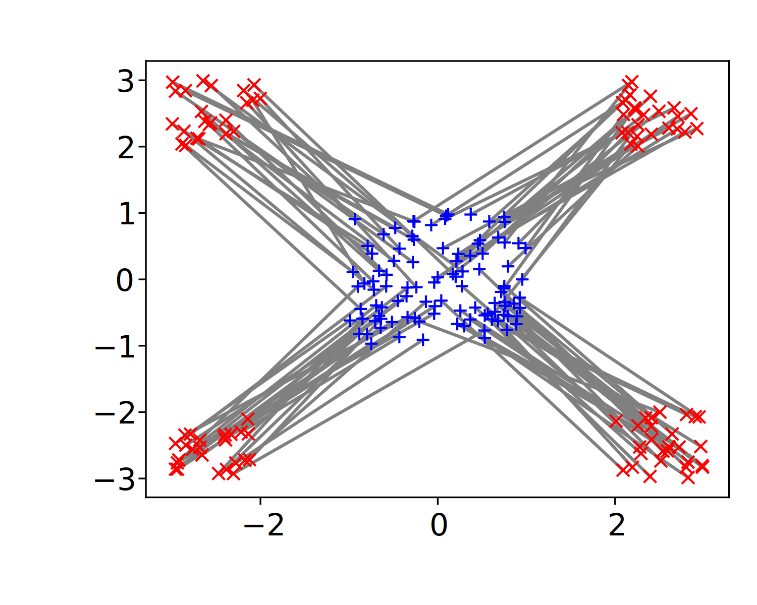
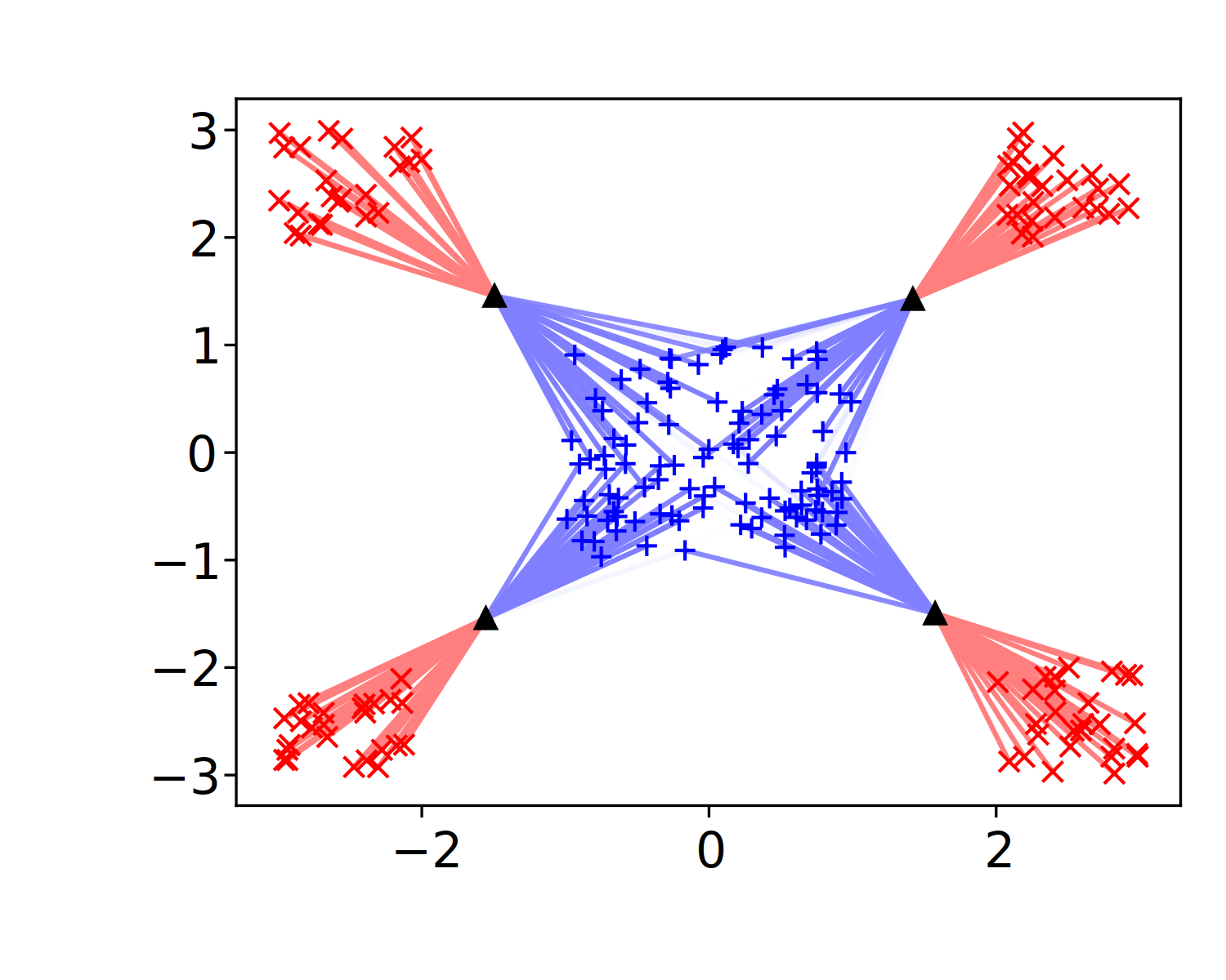
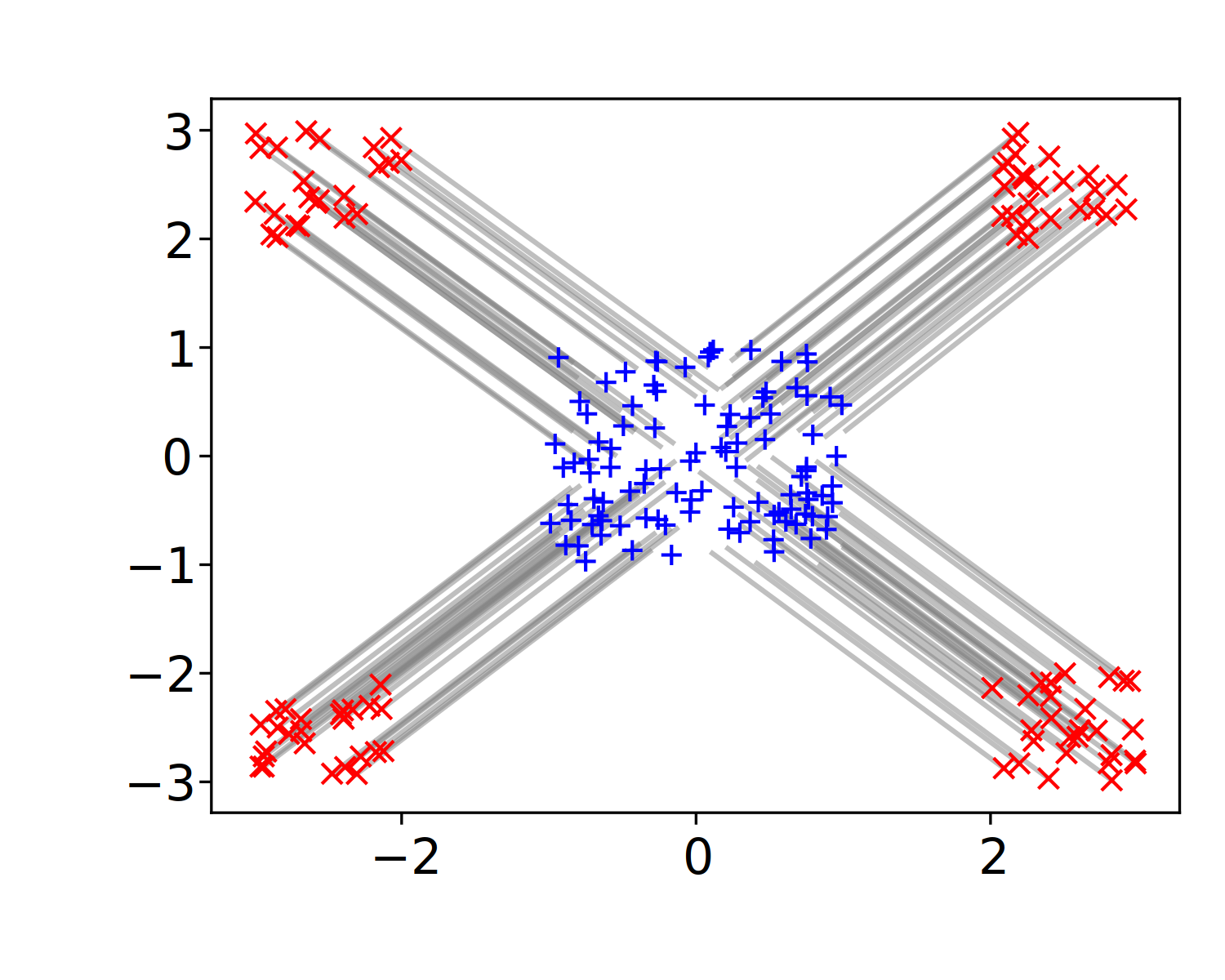
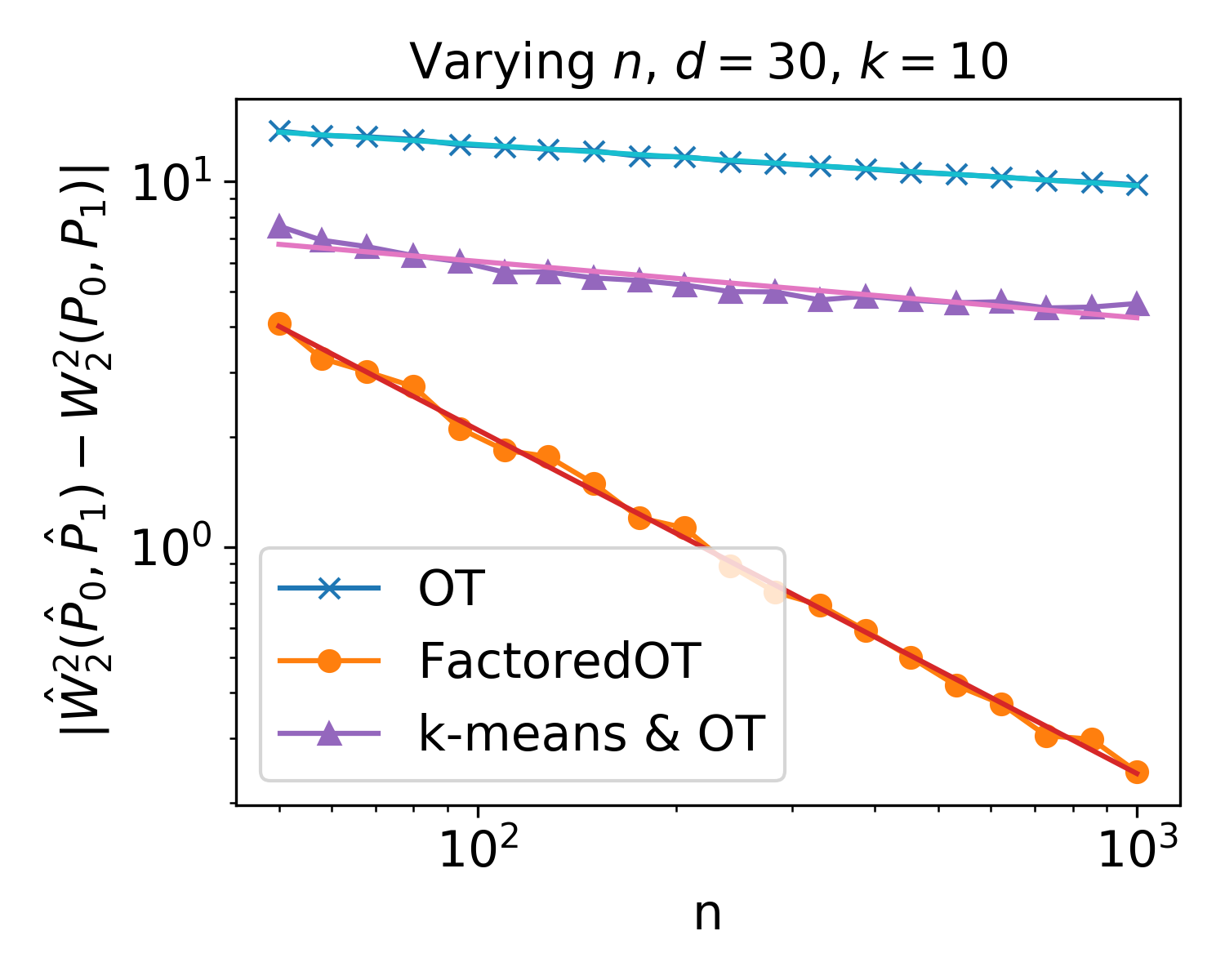
We consider $P_{0}=\textsf{Unif}([-1,1]^{d})$, the uniform distribution on a hypercube in dimension $d$ and $P_{1}=T_{\#}(P_{0})$, the push-forward of $P_{0}$ under a map $T$, defined as the distribution of $Y=T(X)$, if $X\sim P_{0}$. We choose $T(X)=X+2\mathop{\mathrm{sign}}(X)\odot(e_{1}+e_{2})$, where the sign is taken element-wise. As can be seen in Figure 1, this splits the cube into four pieces which drift away. This map is the subgradient of a convex function and hence an optimal transport map by Brenier’s Theorem [Villani, 2003, Theorem 2.12]. This observation allows us to compute explicitly $W_{2}^{2}(P_{0},P_{1})=8$. We compare the results of computing optimal transport on samples and the associated empirical optimal transport cost with the estimator (7), as well as with a simplified procedure that consists in first performing $k$-means on both $\hat{P}_{0}$ and $\hat{P}_{1}$ and subsequently calculating the $W_{2}$ distance between the centroids.

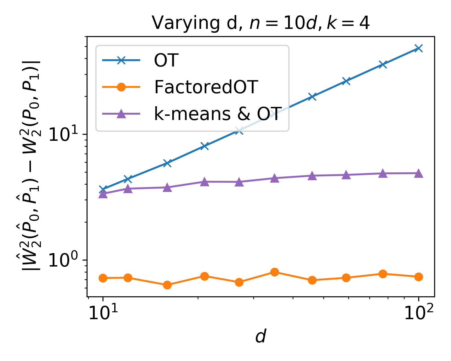
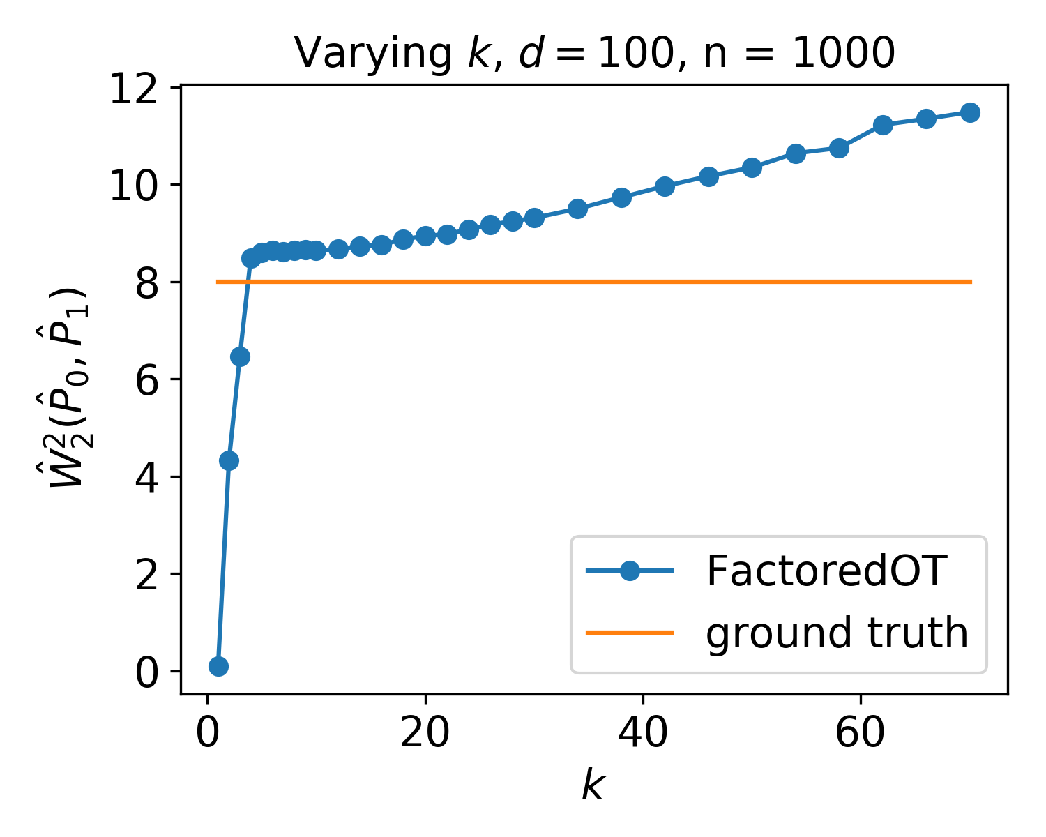
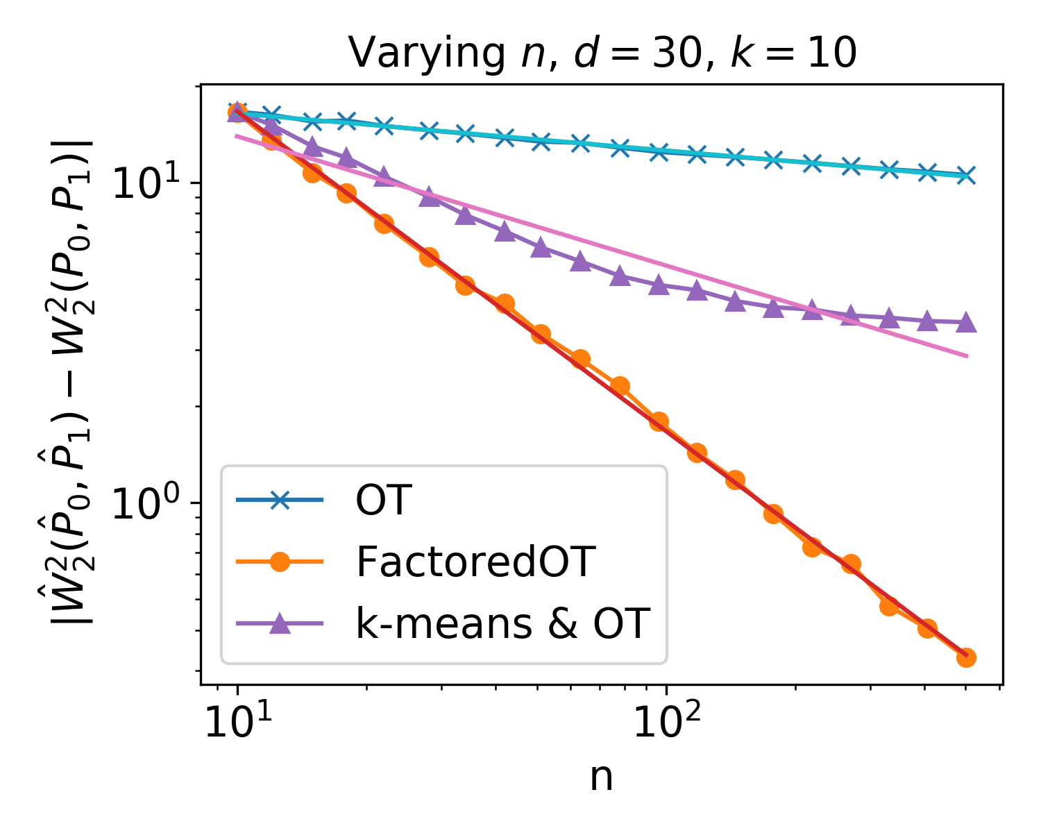
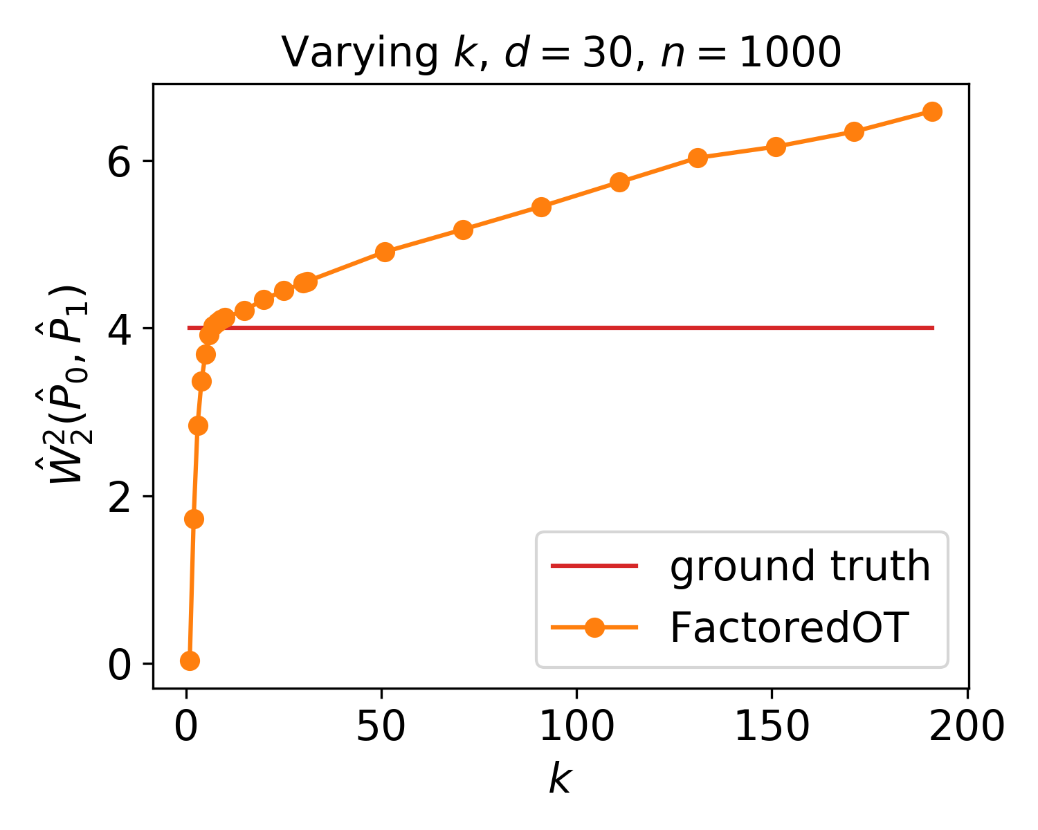
The bottom left subplot of Figure 1 shows that FactoredOT provides a substantially better estimate of the $W_{2}$ distance compared to the empirical optimal transport cost, especially in terms of its scaling with the sample size. Moreover, from the bottom center subplot of the same figure, we deduce that a linear scaling of samples with respect to the dimension is enough to guarantee bounded error, while in the case of an empirical coupling, we see a growing error. Finally, the bottom right plot indicates that the estimator is rather stable to the choice of $k$ above a minimum threshold. We suggest choosing $k$ to match this threshold.

Disk to annulus

To show the robustness of our estimator in the case where the ground truth Wasserstein distance is not exactly the cost of a factored coupling, we calculate the optimal transport between the uniform measures on a disk and on an annulus. In order to turn this into a high-dimensional problem, we consider the 2D disk and annulus as embedded in $d$ dimensions and extend both source and target distribution to be independent and uniformly distributed on the remaining $d-2$ dimensions. In other words, we set

$$\begin{aligned} P_{0}=\textsf{Unif}(\{x\in\mathbb{R}^{d}:{}&\|(x_{1},x_{2})\|_{2}\leq 1,\\ &x_{i}\in[0,1]\text{ for }i=3,\dots,d\})\\ \end{aligned}$$

$$\begin{aligned} P_{1}=\textsf{Unif}(\{x\in\mathbb{R}^{d}:{}&2\leq\|(x_{1},x_{2})\|_{2}\leq 3,\\ &x_{i}\in[0,1]\text{ for }i=3,\dots,d\})\end{aligned}$$

Figure 2 shows that the performance is similar to that obtained for the fragmenting hypercube.

6.2 Batch correction for single cell RNA data

The advent of single cell RNA sequencing is revolutionizing biology with a data deluge. Biologists can now quantify the cell types that make up different tissues and quantify the molecular changes that govern development (reviewed in Wagner et al. [2016] and Kolodziejczyk et al. [2015]). As data is collected by different labs, and for different organisms, there is an urgent need for methods to robustly integrate and align these different datasets [Butler et al., 2018, Haghverdi et al., 2018, Crow et al., 2018].

Cells are represented mathematically as points in a several-thousand dimensional vector space, with a dimension for each gene. The value of each coordinate represents the expression-level of the corresponding gene. Here we show that optimal transport achieves state of the art results for the task of aligning single cell datasets. We align a pair of haematopoietic datasets collected by different scRNA-seq protocols in different laboratories (as described in Haghverdi et al. [2018]). We quantify performance by measuring the fidelity of cell-type label transfer across data sets. This information is available as ground truth in both datasets, but is not involved in computing the alignment.

Figure 3: Domain adaptation for scRNA-seq. Both source and target data set are subsampled (50 cells/type) and colored by cell type. Empty circles indicate the inferred label with 20NN classification after FactoredOT.

Table 1: Mean mis-classification percentage (Error) and standard deviation (Std) for scRNA-Seq batch correction

Method	Error	Std
FOT	14.10	$4.44$
MNN	$17.53$	$5.09$
OT	$17.47$	$3.17$
OT-ER	$18.58$	$6.57$
OT-L1L2	$15.47$	$5.35$
kOT	$15.37$	$4.76$
SA	$15.10$	$3.14$
TCA	$24.57$	$7.04$
NN	$21.98$	$4.90$

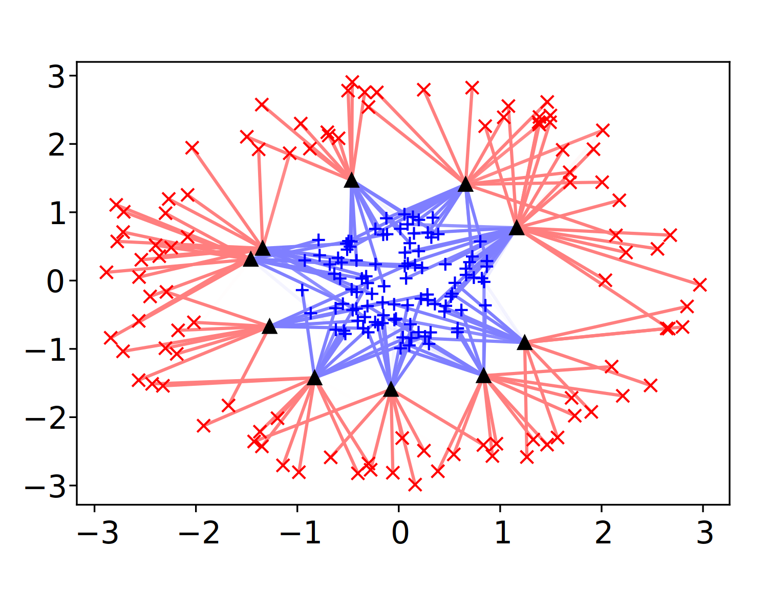
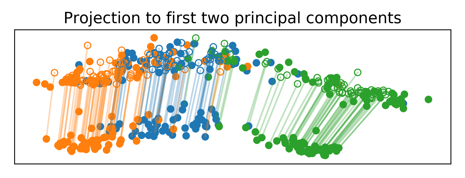
We compare the performance of FactoredOT (FOT) to the following baselines: (a) independent majority vote on k nearest neighbors in the target set (NN), (b) optimal transport (OT), (c) entropically regularized optimal transport (OT-ER), (d) OT with group lasso penalty (OT-L1L2) [Courty et al., 2014], (e) two-step method in which we first perform $k$-means and then perform optimal transport on the $k$-means centroids (kOT), (f) Subspace Alignment (SA) [Fernando et al., 2013], (g) Transfer Component Analysis (TCA) [Pan et al., 2011], and (h) mutual nearest neighbors (MNN) [Haghverdi et al., 2018]. After projecting the source data onto the target set space, we predict the label of each of the source single cells by using a majority vote over the 20 nearest neighbor single cells in the target dataset (see Figure 3 for an example). FactoredOT outperforms the baselines for this task, as shown in Table 1, where we report the percentage of mislabeled data.

7 DISCUSSION

In this paper, we make a first step towards statistical regularization of optimal transport with the objective of both estimating the Wasserstein distance and the optimal coupling between two probability distributions. Our proposed methodology generically applies to various tasks associated to optimal transport, leads to a good estimator of the Wasserstein distance even in high dimension, and is also competitive with state-of-the-art domain adaptation techniques. Our theoretical results demonstrate that the curse of dimensionality in statistical optimal transport can be overcome by imposing structural assumptions. This is an encouraging step towards the deployment of optimal transport as a tool for high-dimensional data analysis.

Statistical regularization of optimal transport remains largely unexplored and many other forms of inductive bias may be envisioned. For example, $k$-means OT used in Section 6 implicitly assumes that marginals are clustered–e.g., coming from a mixture of Gaussians. In this work we opt for a regularization of the optimal coupling itself, which could be accomplished in other ways. Indeed, while Theorem 4 indicates that factored couplings overcome the curse of dimensionality, latent distributions with infinite support but low complexity are likely to lead to similar improvements.

Appendix A Proof of Proposition 4.2

By the identification in Proposition 4.1, we have $\gamma=\sum_{j=1}^{k}\frac{1}{\lambda_{j}}C_{j}^{0}\otimes C_{j}^{1}$. We perform a bias-variance decomposition:

$$\int\|x-y\|^{2}\,\mathrm{d}\gamma(x,y)$$

$$={} \sum_{j=1}^{k}\frac{1}{\lambda_{j}}\int\|x-y\|^{2}\,\mathrm{d}C_{j}^{0}(x)\mathrm{d}C_{j}^{1}(y)$$

$$={} \sum_{j=1}^{k}\frac{1}{\lambda_{j}}\int\|x-\mu(C_{j}^{0})-(y-\mu(C_{j}^{1}))+(\mu(C_{j}^{0})-\mu(C_{j}^{1}))\|^{2}\,\mathrm{d}C_{j}^{0}(x)\mathrm{d}C_{j}^{1}(y)$$

$$={} \sum_{j=1}^{k}\int\|x-\mu(C_{j}^{0})\|^{2}\,\mathrm{d}C_{j}^{0}(x)+\int\|y-\mu(C_{j}^{1})\|^{2}\mathrm{d}C_{j}^{1}(y)+\lambda_{j}\|\mu(C_{j}^{0})-\mu(C_{j}^{1})\|^{2}\,,$$

where the cross terms vanish by the definition of $\mu(C_{j}^{0})$ and $\mu(C_{j}^{1})$. ∎

Appendix B Proof of Proposition 4.3

We first show that if $H$ is an optimal solution to (6), then the hubs $z_{1},\dots,z_{k}$ satisfy $z_{j}=\frac{1}{2}(\mu(C_{j}^{0})+\mu(C_{j}^{1}))$ for $j=1,\dots k$. Let $P$ be any distribution in $\mathcal{D}_{k}$. Denote the support of $P$ by $z_{1},\dots,z_{k}$, and let $\{C_{j}^{0}\},\{C_{j}^{1}\}$ be the partition of $\hat{P}_{0}$ and $\hat{P}_{1}$ induced by the objective $W_{2}^{2}(P,\hat{P}_{0})+W_{2}^{2}(P,\hat{P}_{1})$. By the same bias-variance decomposition as in the proof of Proposition 4.2,

$$W_{2}^{2}(\hat{P}_{0},P)=\sum_{j=1}^{k}\int_{C_{j}^{0}}\|x-z_{j}\|^{2}\,\mathrm{d}\hat{P}_{0}(x)=\sum_{j=1}^{k}\int_{C_{j}^{0}}\|x-\mu(C_{j}^{0})\|^{2}\,\mathrm{d}\hat{P}_{0}(x)+\lambda_{j}\|z_{j}-\mu(C_{j}^{0})\|^{2}\,,$$

and since the analogous claim holds for $\hat{P}_{1}$, we obtain that

$$W_{2}^{2}(P,\hat{P}_{0})+W_{2}^{2}(P,\hat{P}_{1})={} \sum_{j=1}^{k}\int_{C_{j}^{0}}\|x-\mu(C_{j}^{0})\|^{2}\,\mathrm{d}\hat{P}_{0}(x)$$

$$+\int_{C_{j}^{1}}\|y-\mu(C_{j}^{1})\|^{2}\,\mathrm{d}\hat{P}_{1}(y)+\lambda_{j}(\|z_{j}-\mu(C_{j}^{0})\|^{2}+\|z_{j}-\mu(C_{j}^{1})\|^{2})\,.$$

The first two terms depend only on the partitions of $\hat{P}_{0}$ and $\hat{P}_{1}$, and examining the final term shows that any minimizer of $W_{2}^{2}(P,\hat{P}_{0})+W_{2}^{2}(P,\hat{P}_{1})$ must have $z_{j}=\frac{1}{2}(\mu(C_{j}^{0})+\mu(C_{j}^{1}))$ for $j=1,\dots k$, where $C_{j}^{0}$ and $C_{j}^{1}$ are induced by $P$, in which case $\|z_{j}-\mu(C_{j}^{0})\|^{2}+\|z_{j}-\mu(C_{j}^{1})\|^{2}=\frac{1}{2}\|\mu(C_{j}^{0})-\mu(C_{j}^{1})\|^{2}$. Minimizing over $P\in\mathcal{D}_{k}$ yields the claim. ∎

Appendix C Proof of Theorem 4

The proof of Theorem 4 relies on the following propositions, which shows that controlling the gap between $W_{2}^{2}(\rho,P)$ and $W_{2}^{2}(\rho,Q)$ is equivalent to controlling the distance between $P$ and $Q$ with respect to a simple integral probability metric [Müller, 1997].

We make the following definition.

Definition 5.

A set $S\in{\rm I}\kern-1.79993pt{\rm R}^{d}$ is a $n$-polyhedron if $S$ can be written as the intersection of $n$ closed half-spaces.

We denote the set of $n$-polyhedra by $\mathcal{P}_{n}$. Given $c\in{\rm I}\kern-1.79993pt{\rm R}^{d}$ and $S\in\mathcal{P}_{k-1}$, define

$$f_{c,S}(x):=\|x-c\|^{2}\mathds{1}_{x\in S}\quad\quad\forall x\in{\rm I}\kern-1.79993pt{\rm R}^{d}\,.$$

Proposition C.1.

Let $P$ and $Q$ be probability measures supported on the unit ball in ${\rm I}\kern-1.79993pt{\rm R}^{d}$. The

$$\sup_{\rho\in\mathcal{D}_{k}}|W^{2}_{2}(\rho,P)-W^{2}_{2}(\rho,Q)|\leq 5k\sup_{c:\|c\|\leq 1,S\in\mathcal{P}_{k-1}}|{\rm I}\kern-1.79993pt{\rm E}_{P}f_{c,S}-{\rm I}\kern-1.79993pt{\rm E}_{Q}f_{c,S}|\,.$$ (9)

To obtain Theorem 4, we use techniques from empirical process theory to control the right side of (9) when $Q=\hat{P}$.

Proposition C.2.

There exists a universal constant $C$ such that, if $P$ is supported on the unit ball and $X_{1},\dots,X_{n}\sim\mu$ are i.i.d., then

$${\rm I}\kern-1.79993pt{\rm E}\sup_{c:\|c\|\leq 1,S\in\mathcal{P}_{k-1}}|{\rm I}\kern-1.79993pt{\rm E}_{P}f_{c,S}-{\rm I}\kern-1.79993pt{\rm E}_{\hat{P}}f_{c,S}|\leq C\sqrt{\frac{kd\log k}{n}}\,.$$ (10)

With these tools in hand, the proof of Theorem 4 is elementary.

Proof of Theorem 4.

Proposition C.1 implies that

$${\rm I}\kern-1.79993pt{\rm E}\sup_{\rho\in\mathcal{D}_{k}}|W_{2}^{2}(\rho,\hat{\mu})-W_{2}^{2}(\rho,\mu)|\lesssim\sqrt{\frac{k^{3}d\log k}{n}}\,.$$

To show the high probability bound, it suffices to apply the bounded difference inequality (see [McDiarmid, 1989]) and note that, if $\hat{P}$ and $\tilde{P}$ differ in the location of a single sample, then for any $\rho$, we have the bound $|W_{2}^{2}(\rho,\hat{P})-W_{2}^{2}(\rho,\tilde{P})|\leq 4/n$. The concentration inequality immediately follows. ∎

We now turn to the proofs of Propositions C.1 and Propositions C.2.

We first review some facts from the literature. It is by now well known that there is an intimate connection between the $k$-means objective and the squared Wasserstein $2$-distance [Pollard, 1982, Ng, 2000, Canas and Rosasco, 2012]. This correspondence is based on the following observation, more details about which can be found in [Graf and Luschgy, 2000]: given fixed points $c_{1},\dots,c_{k}$ and a measure $P$, consider the quantity

$$\min_{w\in\Delta_{k}}W_{2}^{2}\Big{(}\sum_{i=1}^{k}w_{i}\delta_{c_{i}},P\Big{)}\,,$$ (11)

where the minimization is taken over all probability vectors $w:=(w_{1},\dots,w_{k})$. Note that, for any measure $\rho$ supported on $\{c_{1},\dots,c_{k}\}$, we have the bound

$$W_{2}^{2}(\rho,P)\geq{\rm I}\kern-1.79993pt{\rm E}\big{[}\min_{i\in[k]}\|X-c_{k}\|^{2}\big{]}\quad\quad X\sim P\,.$$

On the other hand, this minimum can be achieved by the following construction. Denote by $\{S_{1},\dots,S_{k}\}$ the Voronoi partition [Okabe et al., 2000] of ${\rm I}\kern-1.79993pt{\rm R}^{d}$ with respect to the centers $\{c_{1},\dots,c_{k}\}$ and let $\rho=\sum_{i=1}^{k}P(S_{i})\delta_{c_{i}}$. If we let $T:{\rm I}\kern-1.79993pt{\rm R}^{d}\to\{c_{1},\dots,c_{k}\}$ be the function defined by $S_{i}=T^{-1}(c_{i})$ for $i\in[k]$, then $(\mathrm{id},T)_{\sharp}P$ defines a coupling between $P$ and $\rho$ which achieves the above minimum, and

$${\rm I}\kern-1.79993pt{\rm E}[\|X-T(X)\|^{2}]={\rm I}\kern-1.79993pt{\rm E}[\min_{i\in[k]}\|X-c_{i}\|^{2}]\quad\quad X\sim P\,.$$

The above argument establishes that the measure closest to $P$ with prescribed support of at most $k$ points is induced by a Voronoi partition of ${\rm I}\kern-1.79993pt{\rm R}^{d}$, and this observation carries over into the context of the $k$-means problem [Canas and Rosasco, 2012], where one seeks to solve

$$\min_{\rho\in\mathcal{D}_{k}}W_{2}^{2}(\rho,P)\,.$$ (12)

The above considerations imply that the minimizing measure will correspond to a Voronoi partition, and that the centers $c_{1},\dots,c_{k}$ will lie at the centroids of each set in the partition with respect to $P$. As above, there will exist a map $T$ realizing the optimal coupling between $P$ and $\rho$, where the sets $T^{-1}(c_{i})$ for $i\in[k]$ form a Voronoi partition of ${\rm I}\kern-1.79993pt{\rm R}^{d}$. In particular, standard facts about Voronoi cells for the $\ell_{2}$ distance [Okabe et al., 2000, Definition V4] imply that, for $i\in[k]$, the set $\operatorname{cl}(T^{-1}(c_{i}))$ is a $(k-1)$-polyhedron. (See Definition 5 above.)

In the case when $\rho$ is an arbitrary measure with support of size $k$—and not the solution to an optimization problem such as (11) or (12)—it is no longer the case that the optimal coupling between $P$ and $\rho$ corresponds to a Voronoi partition of ${\rm I}\kern-1.79993pt{\rm R}^{d}$. The remainder of this section establishes, however, that, if $P$ is absolutely continuous with respect to the Lebgesgue measure, then there does exist a map $T$ such that the fibers of points in the image of $T$ have a particularly simple form: like Voronoi cells, the sets $\{\operatorname{cl}(T^{-1}(c_{i})\}_{i=1}^{k}$ can be taken to be simple polyehdra.

Definition 6.

A function $T:{\rm I}\kern-1.79993pt{\rm R}^{d}\to{\rm I}\kern-1.79993pt{\rm R}^{d}$ is a polyhedral quantizer of order $k$ if $T$ takes at most $k$ values and if, for each $x\in\mathrm{Im}(T)$, the set $\operatorname{cl}(T^{-1}(x))$ is a $(k-1)$-polyhedron and $\partial T^{-1}(x)$ has zero Lebesgue measure.

We denote by $\mathcal{Q}_{k}$ the set of $k$-polyhedral quantizers whose image lies inside the unit ball of ${\rm I}\kern-1.79993pt{\rm R}^{d}$.

Proposition C.3.

Let $P$ be any absolutely continuous measure in ${\rm I}\kern-1.79993pt{\rm R}^{d}$, and let $\rho$ be any measure supported on $k$ points. Then there exists a map $T$ such that $(id,T)_{\sharp}P$ is an optimal coupling between $P$ and $\rho$ and $T$ is a polyhedral quantizer of order $k$.

Proof.

Denote by $\rho_{1},\dots,\rho_{k}$ the support of $\rho$. Standard results in optimal transport theory [Santambrogio, 2015, Theorem 1.22] imply that there exists a convex function $u$ such that the optimal coupling between $P$ and $\rho$ is of the form $(\mathrm{id},\nabla u)_{\sharp}P$. Let $S_{i}=(\nabla u)^{-1}(\rho_{i})$.

Since $\nabla u(x)=\rho_{j}$ for any $x\in S_{j}$, the restriction of $u$ to $S_{j}$ must be an affine function. We obtain that there exists a constant $\beta_{j}$ such that

$$u(x)=\langle\rho_{j},x\rangle+\beta_{j}\quad\quad\forall x\in S_{j}\,.$$

Since $\rho_{j}$ has nonzero mass, the fact that $\nabla u_{\sharp}P=\rho$ implies that $P(S_{j})>0$, and, since $P$ is absolutely continuous with respect to the Lebesgue measure, this implies that $S_{j}$ has nonempty interior. If $x\in\operatorname{int}(S_{j})$, then $\partial u(x)=\{\rho_{j}\}$. Equivalently, for all $y\in{\rm I}\kern-1.79993pt{\rm R}^{d}$,

$$u(y)\geq\langle\rho_{j},y\rangle+\beta_{j}\,.$$

Employing the same argument for all $j\in[k]$ yields

$$u(x)\geq\max_{j\in[k]}\langle\rho_{j},x\rangle+\beta_{j}\,.$$

On the other hand, if $x\in S_{i}$, then

$$u(x)=\langle\rho_{i},x\rangle+\beta_{i}\leq\max_{j\in[k]}\langle\rho_{j},x\rangle+\beta_{j}\,.$$

We can therefore take $u$ to be the convex function

$$u(x)=\max_{j\in[k]}\langle\rho_{j},x\rangle+\beta_{j}\,,$$

which implies that, for $i\in[k]$,

$$\operatorname{cl}(S_{i}) =\{y\in{\rm I}\kern-1.79993pt{\rm R}^{d}:\langle\rho_{i},x\rangle+\beta_{i}\geq\langle\rho_{j},x\rangle+\beta_{j}\quad\forall j\in[k]\setminus\{i\}\}$$

$$=\bigcap_{j\neq i}\{y\in{\rm I}\kern-1.79993pt{\rm R}^{d}:\langle\rho_{i},x\rangle+\beta_{i}\geq\langle\rho_{j},x\rangle+\beta_{j}\}\,.$$

Therefore $\operatorname{cl}(S_{i})$ can be written as the intersection of $k-1$ halfspaces. Moreover, $\partial S_{i}\subseteq\bigcup_{j\neq i}\{y\in{\rm I}\kern-1.79993pt{\rm R}^{d}:\langle\rho_{i},x\rangle+\beta_{i}=\langle\rho_{j},x\rangle+\beta_{j}\}$, which has zero Lebesgue measure, as claimed. ∎

C.1 Proof of Proposition C.1

By symmetry, it suffices to show the one-sided bound

$$\sup_{\rho\in\mathcal{D}_{k}}W^{2}_{2}(\rho,Q)-W^{2}_{2}(\rho,P)\leq 5k\sup_{c:\|c\|\leq 1,S\in\mathcal{P}_{k-1}}|{\rm I}\kern-1.79993pt{\rm E}_{P}f_{c,S}-{\rm I}\kern-1.79993pt{\rm E}_{Q}f_{c,S}|\,.$$

We first show the claim for $P$ and $Q$ which are absolutely continuous. Fix a $\rho\in\mathcal{D}_{k}$. Since $P$ and $Q$ are absolutely continuous, we can apply Proposition C.3 to obtain that there exists a $T\in\mathcal{Q}_{k}$ such that

$$W_{2}^{2}(\rho,P)={\rm I}\kern-1.79993pt{\rm E}_{P}\|X-T(X)\|^{2}\,.$$

Let $\{c_{1},\dots,c_{k}\}$ be the image of $T$, and for $i\in[k]$ let $S_{i}:=\operatorname{cl}(T^{-1}(c_{i}))$. Denote by $d_{TV}(\mu,\nu):=\sup_{\text{$A$ measurable}}|\mu(A)-\nu(A)|$ the total variation distance between $\mu$ and $\nu$. Applying Lemma E.1 to $\rho$ and $Q$ yields that

$$W_{2}^{2}(Q,\rho)\leq{\rm I}\kern-1.79993pt{\rm E}_{Q}\|X-T(X)\|^{2}+4\mathrm{d_{TV}}(T_{\sharp}Q,\rho)\,.$$

Since $\rho=T_{\sharp}P$ and $Q$ and $P$ are absolutely continuous with respect to the Lebesgue measure, we have

$$\mathrm{d_{TV}}(T_{\sharp}Q,\rho) =\mathrm{d_{TV}}(T_{\sharp}Q,T_{\sharp}P)$$

$$=\frac{1}{2}\sum_{i=1}^{k}|P(T^{-1}(c_{i}))-Q(T^{-1}(c_{i}))|$$

$$=\frac{1}{2}\sum_{i=1}^{k}|P(S_{i})-Q(S_{i})|\,.$$

Combining the above bounds yields

$$W_{2}^{2}(\rho,Q)-W_{2}^{2}(\rho,P) \leq{\rm I}\kern-1.79993pt{\rm E}_{Q}\|X-T(X)\|^{2}-{\rm I}\kern-1.79993pt{\rm E}_{P}\|X-T(X)\|^{2}+2\sum_{i=1}^{k}|P(S_{i})-Q(S_{i})|$$

$$\leq\sum_{i=1}^{k}|{\rm I}\kern-1.79993pt{\rm E}_{Q}\|X-c_{i}\|^{2}\mathds{1}_{X\in S_{i}}-{\rm I}\kern-1.79993pt{\rm E}_{P}\|X-c_{i}\|^{2}\mathds{1}_{X\in S_{i}}|+2|P(S_{i})-Q(S_{i})|$$

$$\leq k\sup_{c,S}\left(|{\rm I}\kern-1.79993pt{\rm E}_{Q}\|X-c\|^{2}\mathds{1}_{X\in S}-{\rm I}\kern-1.79993pt{\rm E}_{P}\|X-c\|^{2}\mathds{1}_{X\in S}|+2|P(S)-Q(S)|\right)$$

$$=k\sup_{c,S}\left(|{\rm I}\kern-1.79993pt{\rm E}_{Q}f_{c,S}-{\rm I}\kern-1.79993pt{\rm E}_{P}f_{c,S}|+2|P(S)-Q(S)|\right)$$

where the supremum is taken over $c\in{\rm I}\kern-1.79993pt{\rm R}^{d}$ satisfying $\|c\|\leq 1$ and $S\in\mathcal{P}_{k-1}$.

If $\|v\|=1$, then

$$\mathds{1}_{X\in S}=\frac{1}{2}(\|X+v\|^{2}+\|X-v\|^{2}-2\|X\|^{2})\mathds{1}_{X\in S}\,,$$

which implies

$$|P(S)-Q(S)| =|{\rm I}\kern-1.79993pt{\rm E}_{P}\mathds{1}_{X\in S}-{\rm I}\kern-1.79993pt{\rm E}_{Q}\mathds{1}_{X\in S}|$$

$$\leq\frac{1}{2}\left(|{\rm I}\kern-1.79993pt{\rm E}_{P}f_{v,S}-{\rm I}\kern-1.79993pt{\rm E}_{Q}f_{v,S}|+|{\rm I}\kern-1.79993pt{\rm E}_{P}f_{-v,S}-{\rm I}\kern-1.79993pt{\rm E}_{Q}f_{-v,S}|+2|{\rm I}\kern-1.79993pt{\rm E}_{P}f_{0,S}-{\rm I}\kern-1.79993pt{\rm E}_{Q}f_{0,S}|\right)$$

$$\leq 2\sup_{c,S}|{\rm I}\kern-1.79993pt{\rm E}_{P}f_{c,S}-{\rm I}\kern-1.79993pt{\rm E}_{Q}f_{c,S}|\,.$$

Combining the above bounds yields

$$W_{2}^{2}(\rho,Q)-W_{2}^{2}(\rho,P)\leq 5k\sup_{c,S}|{\rm I}\kern-1.79993pt{\rm E}_{P}f_{c,S}-{\rm I}\kern-1.79993pt{\rm E}_{Q}f_{c,S}|$$

Finally, since this bound holds for all $\rho\in\mathcal{D}_{k}$, taking the supremum of the left side yields the claim for absolutely continuous $P$ and $Q$.

To prove the claim for arbitrary measures, we reduce to the absolutely continuous case. Let $\delta\in(0,1)$ be arbitrary, and let $\mathcal{K}_{\delta}$ be any absolutely continuous probability measure such that, if $Z\sim\mathcal{K}_{\delta}$ then $\|Z\|\leq\delta$ almost surely. Let $\rho\in\mathcal{D}_{k}$. The triangle inequality for $W_{2}$ implies

$$|W_{2}(\rho,Q)-W_{2}(\rho,Q*\mathcal{K}_{\delta})|\leq W_{2}(Q,Q*\mathcal{K}_{\delta})\leq\delta\,,$$

where the final inequality follows from the fact that, if $X\sim Q$ and $Z\sim\mathcal{K}_{\delta}$, then $W^{2}_{2}(Q,Q*\mathcal{K}_{\delta})\leq{\rm I}\kern-1.79993pt{\rm E}\|X-(X+Z)\|^{2}\leq\delta^{2}$. Since $\rho$ and $Q$ are both supported on the unit ball, the trivial bound $W_{2}(\rho,Q)\leq 2$ holds. If $\delta\leq 1$, then $W_{2}(\rho,Q*\mathcal{K}_{\delta})\leq 3$, and we obtain

$$|W_{2}^{2}(\rho,Q)-W_{2}^{2}(\rho,Q*\mathcal{K}_{\delta})|\leq 5\delta\,.$$

The same argument implies

$$|W_{2}^{2}(\rho,P)-W_{2}^{2}(\rho,P*\mathcal{K}_{\delta})|\leq 5\delta\,.$$

Therefore

$$\sup_{\rho\in\mathcal{D}_{K}}W^{2}_{2}(\rho,Q)-W^{2}_{2}(\rho,P)\leq\sup_{\rho\in\mathcal{D}_{K}}W^{2}_{2}(\rho,Q*\mathcal{K}_{\delta})-W^{2}_{2}(\rho,P*\mathcal{K}_{\delta})+10\delta\,.$$

Likewise, for any $x$ and $c$ in the unit ball, if $\|z\|\leq\delta$, then by the exact same argument as was used above to bound $|W_{2}^{2}(\rho,Q)-W_{2}^{2}(\rho,Q*\mathcal{K}_{\delta})|$, we have

$$|f_{c,S}(x+z)-f_{c,S-z}(x)|\leq 5\delta\,.$$

Let $Z\sim\mathcal{K}_{\delta}$ be independent of all other random variables, and denote by ${\rm I}\kern-1.79993pt{\rm E}_{Z}$ expectation with respect to this quantity. Now, applying the proposition to the absolutely continuous measures $P*\mathcal{K}_{\delta}$ and $Q*\mathcal{K}_{\delta}$, we obtain

$$\sup_{\rho\in\mathcal{D}_{k}}W^{2}_{2}(\rho,Q)-W^{2}_{2}(\rho,P) \leq 5k\sup_{c,S}\left|{\rm I}\kern-1.79993pt{\rm E}_{Z}\left[{\rm I}\kern-1.79993pt{\rm E}_{P}f_{c,S}(X+Z)-{\rm I}\kern-1.79993pt{\rm E}_{Q}f_{c,S}(X+Z)\right]\right|+10\delta$$

$$\leq{\rm I}\kern-1.79993pt{\rm E}_{Z}\Big{[}5k\sup_{c,S}|{\rm I}\kern-1.79993pt{\rm E}_{P}f_{c,S}(X+Z)-{\rm I}\kern-1.79993pt{\rm E}_{Q}f_{c,S}(X+Z)|\Big{]}+10\delta$$

$$\leq{\rm I}\kern-1.79993pt{\rm E}_{Z}\Big{[}5k\sup_{c,S}|{\rm I}\kern-1.79993pt{\rm E}_{P}f_{c,S-Z}-{\rm I}\kern-1.79993pt{\rm E}_{Q}f_{c,S-Z}|\Big{]}+20\delta\,.$$

It now suffices to note that, for any $S\in\mathcal{P}_{k-1}$ and any $z\in{\rm I}\kern-1.79993pt{\rm R}^{d}$, the set $S-z\in\mathcal{P}_{k-1}$. In particular, this implies that

$$z\mapsto\sup_{c,S}|{\rm I}\kern-1.79993pt{\rm E}_{P}f_{c,S-z}-{\rm I}\kern-1.79993pt{\rm E}_{Q}f_{c,S-z}|$$

is constant, so that the expectation with respect to $Z$ can be dropped.

We have shown that, for any $\delta\in(0,1)$, the bound

$$\sup_{\rho\in\mathcal{D}_{K}}W^{2}_{2}(\rho,P)-W^{2}_{2}(\rho,Q) \leq 5k\sup_{c,S}|{\rm I}\kern-1.79993pt{\rm E}_{P}f_{c,S}-{\rm I}\kern-1.79993pt{\rm E}_{Q}f_{c,S}|+20\delta$$

holds. Taking the infimum over $\delta>0$ yields the claim.∎

Appendix D Proof of Proposition C.2

In this proof, the symbol $C$ will stand for a universal constant whose value may change from line to line. For convenience, we will use the notation $\sup_{c,S}$ to denote the supremum over the feasible set $c:\|c\|\leq 1,S\in\mathcal{P}_{k-1}$.

We employ the method of [Maurer and Pontil, 2010]. By a standard symmetrization argument [Giné and Nickl, 2016], if $g_{1},\dots,g_{n}$ are i.i.d. standard Gaussian random variables, then the quantity in question is bounded from above by

$$\frac{\sqrt{2\pi}}{n}{\rm I}\kern-1.79993pt{\rm E}\sup_{c,S}\left|\sum_{i=1}^{n}g_{i}f_{c,S}(X_{i})\right|\leq\frac{\sqrt{8\pi}}{n}{\rm I}\kern-1.79993pt{\rm E}\sup_{c,S}\sum_{i=1}^{n}g_{i}f_{c,S}(X_{i})+\frac{C}{\sqrt{n}}\,.$$

Given $c$ and $c^{\prime\prime}$ in the unit ball and $S,S^{\prime}\in\mathcal{P}_{k-1}$, consider the increment $(f_{c,S}(x)-f_{c^{\prime},S^{\prime}}(x))^{2}$. If $x\in S\triangle S^{\prime}$ and $\|x\|\leq 1$, then

$$(f_{c,S}(x)-f_{c^{\prime},S^{\prime}}(x))^{2} \leq\max\left\{\|x-c\|^{4},\|x-c^{\prime}\|^{4}\right\}\leq 16\,.$$

On the other hand, if $x\notin S\triangle S^{\prime}$, then

$$(f_{c,S}(x)-f_{c^{\prime},S^{\prime}}(x))^{2} \leq(\|x-c\|^{2}-\|x-c^{\prime}\|^{2})^{2}\,.$$

Therefore, for any $x$ in the unit ball,

$$(f_{c,S}(x)-f_{c^{\prime},S^{\prime}}(x))^{2}\leq 16(\mathds{1}_{x\in S}-\mathds{1}_{x\in S^{\prime}})^{2}+(\|x-c\|^{2}-\|x-c^{\prime}\|^{2})^{2}\,.$$

This fact implies that the Gaussian processes

$$G_{c,S} :=\sum_{i=1}^{n}g_{i}f_{c,S}(X_{i})\quad\quad g_{i}\sim\mathcal{N}(0,1)\text{ i.i.d}$$

$$H_{c,S} :=\sum_{i=1}^{n}4g_{i}\mathds{1}_{X_{i}\in S}+g_{i}^{\prime}\|X_{i}-c\|^{2}\quad\quad g_{i},g_{i}^{\prime}\sim\mathcal{N}(0,1)\text{ i.i.d}\,,$$

satisfy

$${\rm I}\kern-1.79993pt{\rm E}(G_{c,S}-G_{c^{\prime},S^{\prime}})^{2}\leq{\rm I}\kern-1.79993pt{\rm E}(H_{c,S}-H_{c^{\prime},S^{\prime}})^{2}\quad\quad\forall c,c^{\prime},S,S^{\prime}\,.$$

Therefore, by the Slepian-Sudakov-Fernique inequality [Slepian, 1962, Sudakov, 1971, Fernique, 1975],

$${\rm I}\kern-1.79993pt{\rm E}\sup_{c,S}\sum_{i=1}^{n}g_{i}f_{c,S}(X_{i}) \leq{\rm I}\kern-1.79993pt{\rm E}\sup_{c,S}\sum_{i=1}^{n}4g_{i}\mathds{1}_{X_{i}\in S}+g_{i}^{\prime}\|X_{i}-c\|^{2}$$

$$\leq{\rm I}\kern-1.79993pt{\rm E}\sup_{S\in\mathcal{P}_{k-1}}4\sum_{i=1}^{n}g_{i}\mathds{1}_{X_{i}\in S}+{\rm I}\kern-1.79993pt{\rm E}\sup_{c:\|c\|\leq 1}\sum_{i=1}^{n}g_{i}\|X_{i}-c\|^{2}\,.$$

We control the two terms separately. The first term can be controlled using the VC dimension of the class $\mathcal{P}_{k-1}$ [Vapnik and Červonenkis, 1971] by a standard argument in empirical process theory (see, e.g., [Giné and Nickl, 2016]). Indeed, using the bound [Dudley, 1978, Lemma 7.13] combined with the chaining technique [Vershynin, 2016] yields

$${\rm I}\kern-1.79993pt{\rm E}\sup_{S\in\mathcal{P}_{k-1}}4\sum_{i=1}^{n}g_{i}\mathds{1}_{X_{i}\in S}\leq C\sqrt{n\mathrm{VC}(\mathcal{P}_{k-1})}\,.$$

By Lemma E.2, $VC(\mathcal{P}_{k-1})\leq Cdk\log k$; hence

$${\rm I}\kern-1.79993pt{\rm E}\sup_{S\in\mathcal{P}_{k-1}}4\sum_{i=1}^{n}g_{i}\mathds{1}_{X_{i}\in S}\leq C\sqrt{ndk\log k}\,.$$

The second term can be controlled as in [Maurer and Pontil, 2010, Lemma 3]:

$${\rm I}\kern-1.79993pt{\rm E}\sup_{c:\|c\|\leq 1}\sum_{i=1}^{n}g_{i}\|X_{i}-c\|^{2} ={\rm I}\kern-1.79993pt{\rm E}\sup_{c:\|c\|\leq 1}\sum_{i=1}^{n}g_{i}(\|X_{i}\|^{2}-2\langle X_{i},c\rangle+\|c\|^{2})$$

$$\leq 2{\rm I}\kern-1.79993pt{\rm E}\sup_{c:\|c\|\leq 1}\sum_{i=1}^{n}g_{i}\langle X_{i},c\rangle+\sup_{c:\|c\|\leq 1}\sum_{i=1}^{n}g_{i}\|c\|^{2}$$

$$\leq 2{\rm I}\kern-1.79993pt{\rm E}\left\|\sum_{i=1}^{n}g_{i}X_{i}\right\|+\left|\sum_{i=1}^{n}g_{i}\right|$$

$$\leq C\sqrt{n}$$

for some absolute constant $C$.

Combining the above bounds yields

$$\frac{\sqrt{8\pi}}{n}{\rm I}\kern-1.79993pt{\rm E}\sup_{c:\|c\|\leq 1,S\in\mathcal{P}_{k-1}}\sum_{i=1}^{n}g_{i}f_{c,S}(X_{i})\leq C\sqrt{\frac{dk\log k}{n}}\,,$$

and the claim follows.∎

Appendix E Additional lemmas

Lemma E.1.

Let $\mu$ and $\nu$ be probability measures on ${\rm I}\kern-1.79993pt{\rm R}^{d}$ supported on the unit ball. If $T:{\rm I}\kern-1.79993pt{\rm R}^{d}\to{\rm I}\kern-1.79993pt{\rm R}^{d}$, then

$$W_{2}^{2}(\mu,\nu)\leq{\rm I}\kern-1.79993pt{\rm E}\|X-T(X)\|^{2}+4\mathrm{d_{TV}}(T_{\sharp}\mu,\nu)\quad\quad X\sim\mu\,.$$

Proof.

If $X\sim\mu$, then $(X,T(X))$ is a coupling between $\mu$ and $T_{\sharp}\mu$. Combining this coupling with the optimal coupling between $T\sharp\mu$ and $\nu$ and applying the gluing lemma [Villani, 2009] yields that there exists a triple $(X,T(X),Y)$ such that $X\sim\mu$, $Y\sim\nu$, and ${\rm I}\kern-1.79993pt{\rm P}[T(X)\neq Y]=\mathrm{d_{TV}}(T_{\sharp}\mu,\nu)$.

$$W_{2}^{2}(\mu,\nu) \leq{\rm I}\kern-1.79993pt{\rm E}[\|X-Y\|^{2}]$$

$$={\rm I}\kern-1.79993pt{\rm E}[\|X-Y\|^{2}\mathds{1}_{T(X)=Y}]+{\rm I}\kern-1.79993pt{\rm E}[\|X-Y\|^{2}\mathds{1}_{T(X)\neq Y}]$$

$$\leq{\rm I}\kern-1.79993pt{\rm E}[\|X-T(X)\|^{2}]+4\mathrm{d_{TV}}(T_{\sharp}\mu,\nu)\,,$$

where the last inequality uses the fact that ${\rm I}\kern-1.79993pt{\rm P}[T(X)\neq Y]=\mathrm{d_{TV}}(T_{\sharp}\mu,\nu)$ and that $\|X-Y\|\leq 2$ almost surely. ∎

Lemma E.2.

The class $\mathcal{P}_{k-1}$ satisfies $\mathrm{VC}(\mathcal{P}_{k-1})\leq Cdk\log k$.

Proof.

The claim follows from two standard results in VC theory:

• The class all half-spaces in dimension $d$ has VC dimension $d+1$ [Devroye et al., 1996, Corollary 13.1].

• If $\mathcal{C}$ has VC dimension at most $n$, then the class $\mathcal{C}_{s}:=\{c_{1}\cap\dots c_{s}:c_{i}\in\mathcal{C}\,\forall i\in[s]\}$ has VC dimension at most $2ns\log(3s)$ [Blumer et al., 1989, Lemma 3.2.3].

Since $\mathcal{P}_{k-1}$ consists of intersections of at most $k-1$ half-spaces, we have

$$\mathrm{VC}(\mathcal{P}_{k-1})\leq 3(d+1)(k-1)\log(3(k-1))\leq Cdk\log k$$

for a universal constant $C$. ∎

Appendix F Details on numerical experiments

In this section we present implementation details for our numerical experiments.

In all experiments, the relative tolerance of the objective value is used as a stopping criterion for FactoredOT. We terminate calculation when this value reached $10^{-6}$.

F.1 Synthetic experiments from Section 6.1

In the synthetic experiments, the entropy parameter was set to $0.1$.

F.2 Single cell RNA-seq batch correction experiments from Section 6.2

We obtained a pair of single cell RNA-seq data sets from Haghverdi et al. [2018]. The first dataset [Nestorowa et al., 2016] was generated using SMART-seq2 protocol [Picelli et al., 2014], while the second dataset [Paul et al., 2015] was generated using the MARS-seq protocol [Jaitin et al., 2014].

We preprocessed the data using the procedure described by Haghverdi et al. [2018] to reduce to 3,491 dimensions.

Nex, we run our domain adaptation procedure. To determine the choice of parameters, we perform cross-validation over $20$ random sub-samples of the data, each containing $100$ random cells of each of the three cell types in both source and target distribution. Performance is then determined by the mis-classification over $20$ independent versions of the same kind of random sub-samples.

For all methods involving entropic regularization (FOT, OT-ER, OT-L1L2), the candidates for the entropy parameter are $\{10^{-3},10^{-2.5},10^{-2},10^{-1.5},10^{-1}\}$.

For FOT and $k$-means OT, the number of clusters is in $\{3,6,9,12,20,30\}$.

For OT-L1L2, the regularization parameter is in $\{10^{-3},10^{-2},10^{-1},1\}$.

For all subspace methods (SA, TCA), the dimensionality is in $\{10,20,\dots,70\}$.

The labels are determined by first adjusting the sample and then performing a majority vote among $20$ nearest neighbors. While similar experiments [Pan et al., 2011, Courty et al., 2014, 2017] employed 1NN classification because it does not require a tuning parameter, we observed highly decreased performance among all considered domain adaptation methods and therefore chose to use a slightly stronger predictor. The results are not sensitive to the choice of $k$ for the $k$NN predictor for $k\approx 20$.

References

- Agueh and Carlier [2011] M. Agueh and G. Carlier. Barycenters in the Wasserstein space. SIAM Journal on Mathematical Analysis, 43(2):904–924, 2011.
- Altschuler et al. [2017] J. Altschuler, J. Weed, and P. Rigollet. Near-linear time approximation algorithms for optimal transport via Sinkhorn iteration. In Advances in Neural Information Processing Systems, pages 1961–1971, 2017.
- Arora et al. [2012] S. Arora, R. Ge, R. Kannan, and A. Moitra. Computing a nonnegative matrix factorization – provably. In Proceedings of the Forty-fourth Annual ACM Symposium on Theory of Computing, STOC ’12, pages 145–162, New York, NY, USA, 2012. ACM. ISBN 978-1-4503-1245-5.
- Bassetti et al. [2006] F. Bassetti, A. Bodini, and E. Regazzini. On minimum Kantorovich distance estimators. Statistics & Probability Letters, 76(12):1298–1302, 2006.
- Benamou et al. [2015] J.-D. Benamou, G. Carlier, M. Cuturi, L. Nenna, and G. Peyré. Iterative bregman projections for regularized transportation problems. SIAM Journal on Scientific Computing, 37(2):A1111–A1138, 2015.
- Blumer et al. [1989] A. Blumer, A. Ehrenfeucht, D. Haussler, and M. K. Warmuth. Learnability and the Vapnik-Chervonenkis dimension. J. Assoc. Comput. Mach., 36(4):929–965, 1989. ISSN 0004-5411. 10.1145/76359.76371. URL https://doi.org/10.1145/76359.76371.
- Bonneel et al. [2011] N. Bonneel, M. Van De Panne, S. Paris, and W. Heidrich. Displacement interpolation using Lagrangian mass transport. In ACM Transactions on Graphics, volume 30, pages 158:1–158:12, 2011.
- Bonneel et al. [2016] N. Bonneel, G. Peyré, and M. Cuturi. Wasserstein barycentric coordinates: Histogram regression using optimal transport. ACM Transactions on Graphics, 35(4), 2016.
- Butler et al. [2018] A. Butler, P. Hoffman, P. Smibert, E. Papalexi, and R. Satija. Integrating single-cell transcriptomic data across different conditions, technologies, and species. Nature biotechnology, 2018.
- Canas and Rosasco [2012] G. Canas and L. Rosasco. Learning probability measures with respect to optimal transport metrics. In Advances in Neural Information Processing Systems, pages 2492–2500, 2012.
- Candès and Plan [2010] E. J. Candès and Y. Plan. Matrix completion with noise. Proceedings of the IEEE, 98(6):925–936, 2010. 10.1109/JPROC.2009.2035722. URL https://doi.org/10.1109/JPROC.2009.2035722.
- Chizat et al. [2016] L. Chizat, G. Peyré, B. Schmitzer, and F.-X. Vialard. Scaling algorithms for unbalanced transport problems. arXiv preprint arXiv:1607.05816, 2016.
- Claici et al. [2018] S. Claici, E. Chien, and J. Solomon. Stochastic Wasserstein barycenters. International Conference on Machine Learning (ICML), to appear, 2018.
- Cohen and Rothblum [1993] J. E. Cohen and U. G. Rothblum. Nonnegative ranks, decompositions, and factorizations of nonnegative matrices. Linear Algebra Appl., 190:149–168, 1993. ISSN 0024-3795. 10.1016/0024-3795(93)90224-C. URL https://doi.org/10.1016/0024-3795(93)90224-C.
- Courty et al. [2014] N. Courty, R. Flamary, and D. Tuia. Domain adaptation with regularized optimal transport. In Joint European Conference on Machine Learning and Knowledge Discovery in Databases, pages 274–289. Springer, 2014.
- Courty et al. [2017] N. Courty, R. Flamary, D. Tuia, and A. Rakotomamonjy. Optimal transport for domain adaptation. IEEE transactions on pattern analysis and machine intelligence, 39(9):1853–1865, 2017.
- Crow et al. [2018] M. Crow, A. Paul, S. Ballouz, Z. J. Huang, and J. Gillis. Characterizing the replicability of cell types defined by single cell rna-sequencing data using metaneighbor. Nature communications, 9(1):884, 2018.
- Cuturi [2013] M. Cuturi. Sinkhorn distances: Lightspeed computation of optimal transport. In Advances in Neural Information Processing Systems, pages 2292–2300, 2013.
- Cuturi and Doucet [2014a] M. Cuturi and A. Doucet. Fast computation of Wasserstein barycenters. In International Conference on Machine Learning, pages 685–693, 2014a.
- Cuturi and Doucet [2014b] M. Cuturi and A. Doucet. Fast computation of Wasserstein barycenters. In Proc. ICML, pages 685–693, 2014b.
- Cuturi and Peyré [2016] M. Cuturi and G. Peyré. A smoothed dual approach for variational Wasserstein problems. SIAM Journal on Imaging Sciences, 9(1):320–343, 2016.
- de Goes et al. [2011] F. de Goes, D. Cohen-Steiner, P. Alliez, and M. Desbrun. An optimal transport approach to robust reconstruction and simplification of 2d shapes. In Computer Graphics Forum, volume 30, pages 1593–1602, 2011.
- de Goes et al. [2012] F. de Goes, K. Breeden, V. Ostromoukhov, and M. Desbrun. Blue noise through optimal transport. ACM Transactions on Graphics, 31(6):171, 2012.
- Devroye et al. [1996] L. Devroye, L. Györfi, and G. Lugosi. A probabilistic theory of pattern recognition, volume 31 of Applications of Mathematics (New York). Springer-Verlag, New York, 1996.
- Dobrić and Yukich [1995] V. Dobrić and J. E. Yukich. Asymptotics for transportation cost in high dimensions. J. Theoret. Probab., 8(1):97–118, 1995. ISSN 0894-9840. 10.1007/BF02213456. URL https://doi.org/10.1007/BF02213456.
- Dudley [1969] R. M. Dudley. The speed of mean Glivenko-Cantelli convergence. Ann. Math. Statist, 40:40–50, 1969. ISSN 0003-4851. 10.1214/aoms/1177697802. URL https://doi.org/10.1214/aoms/1177697802.
- Dudley [1978] R. M. Dudley. Central limit theorems for empirical measures. Ann. Probab., 6(6):899–929 (1979), 1978. ISSN 0091-1798. URL http://links.jstor.org/sici?sici=0091-1798(197812)6:6<899:CLTFEM>2.0.CO;2-O&origin=MSN.
- Fernando et al. [2013] B. Fernando, A. Habrard, M. Sebban, and T. Tuytelaars. Unsupervised visual domain adaptation using subspace alignment. In Computer Vision (ICCV), 2013 IEEE International Conference On, pages 2960–2967. IEEE, 2013.
- Fernique [1975] X. Fernique. Regularité des trajectoires des fonctions aléatoires gaussiennes. pages 1–96. Lecture Notes in Math., Vol. 480, 1975.
- Ferradans et al. [2014] S. Ferradans, N. Papadakis, G. Peyré, and J.-F. Aujol. Regularized discrete optimal transport. SIAM Journal on Imaging Sciences, 7(3):1853–1882, 2014.
- Frogner et al. [2015] C. Frogner, C. Zhang, H. Mobahi, M. Araya, and T. A. Poggio. Learning with a Wasserstein loss. In Advances in Neural Information Processing Systems, pages 2044–2052, 2015.
- Gao and Kleywegt [2016] R. Gao and A. J. Kleywegt. Distributionally robust stochastic optimization with Wasserstein distance. arXiv:1604.02199, 2016.
- Gao and Church [2005] Y. Gao and G. Church. Improving molecular cancer class discovery through sparse non-negative matrix factorization. Bioinformatics, 21(21):3970–3975, 2005.
- Genevay et al. [2016] A. Genevay, M. Cuturi, G. Peyré, and F. Bach. Stochastic optimization for large-scale optimal transport. In Advances in Neural Information Processing Systems, pages 3440–3448, 2016.
- Genevay et al. [2017] A. Genevay, G. Peyré, and M. Cuturi. Sinkhorn-autodiff: Tractable Wasserstein learning of generative models. arXiv:1706.00292, 2017.
- Giné and Nickl [2016] E. Giné and R. Nickl. Mathematical foundations of infinite-dimensional statistical models. Cambridge Series in Statistical and Probabilistic Mathematics, [40]. Cambridge University Press, New York, 2016. ISBN 978-1-107-04316-9. 10.1017/CBO9781107337862. URL https://doi.org/10.1017/CBO9781107337862.
- Gong et al. [2012] B. Gong, Y. Shi, F. Sha, and K. Grauman. Geodesic flow kernel for unsupervised domain adaptation. In Proc. CVPR, pages 2066–2073. IEEE, 2012.
- Graf and Luschgy [2000] S. Graf and H. Luschgy. Foundations of quantization for probability distributions, volume 1730 of Lecture Notes in Mathematics. Springer-Verlag, Berlin, 2000. ISBN 3-540-67394-6. 10.1007/BFb0103945. URL https://doi.org/10.1007/BFb0103945.
- Gramfort et al. [2015] A. Gramfort, G. Peyré, and M. Cuturi. Fast optimal transport averaging of neuroimaging data. In Information Processing in Medical Imaging, pages 261–272, 2015.
- Haghverdi et al. [2017] L. Haghverdi, A. T. Lun, M. D. Morgan, and J. C. Marioni. Correcting batch effects in single-cell rna sequencing data by matching mutual nearest neighbours. bioRxiv, page 165118, 2017.
- Haghverdi et al. [2018] L. Haghverdi, A. T. Lun, M. D. Morgan, and J. C. Marioni. Batch effects in single-cell rna-sequencing data are corrected by matching mutual nearest neighbors. Nature biotechnology, 2018.
- Jaitin et al. [2014] D. A. Jaitin, E. Kenigsberg, H. Keren-Shaul, N. Elefant, F. Paul, I. Zaretsky, A. Mildner, N. Cohen, S. Jung, A. Tanay, et al. Massively parallel single-cell rna-seq for marker-free decomposition of tissues into cell types. Science, 343(6172):776–779, 2014.
- Kolodziejczyk et al. [2015] A. A. Kolodziejczyk, J. K. Kim, V. Svensson, J. C. Marioni, and S. A. Teichmann. The technology and biology of single-cell rna sequencing. Molecular cell, 58(4):610–620, 2015.
- Kusner et al. [2015] M. Kusner, Y. Sun, N. Kolkin, and K. Q. Weinberger. From word embeddings to document distances. In Proc. ICML, pages 957–966, 2015.
- Lee and Seung [2001] D. D. Lee and H. S. Seung. Algorithms for non-negative matrix factorization. In T. K. Leen, T. G. Dietterich, and V. Tresp, editors, Advances in Neural Information Processing Systems 13, pages 556–562. MIT Press, 2001.
- Liu et al. [2010] G. Liu, Z. Lin, and Y. Yu. Robust subspace segmentation by low-rank representation. In J. Fürnkranz and T. Joachims, editors, Proceedings of the 27th International Conference on Machine Learning (ICML-10), June 21-24, 2010, Haifa, Israel, pages 663–670. Omnipress, 2010. URL http://www.icml2010.org/papers/521.pdf.
- Lloyd [1982] S. P. Lloyd. Least squares quantization in PCM. IEEE Trans. Inform. Theory, 28(2):129–137, 1982. ISSN 0018-9448. 10.1109/TIT.1982.1056489. URL https://doi.org/10.1109/TIT.1982.1056489.
- Ma et al. [2014] J. Ma, Q. Z. Sheng, L. Yao, Y. Xu, and A. Shemshadi. Keyword search over web documents based on earth mover’s distance. In Web Information Systems Engineering, pages 256–265. 2014.
- Markovsky and Usevich [2012] I. Markovsky and K. Usevich. Low rank approximation. Springer, 2012.
- Maurer and Pontil [2010] A. Maurer and M. Pontil. -dimensional coding schemes in Hilbert spaces. IEEE Trans. Inform. Theory, 56(11):5839–5846, 2010. ISSN 0018-9448. 10.1109/TIT.2010.2069250. URL https://doi.org/10.1109/TIT.2010.2069250.
- McDiarmid [1989] C. McDiarmid. On the method of bounded differences. In Surveys in combinatorics, 1989 (Norwich, 1989), volume 141 of London Math. Soc. Lecture Note Ser., pages 148–188. Cambridge Univ. Press, Cambridge, 1989.
- Monge [1781] G. Monge. Mémoire sur la théorie des déblais et des remblais. Mém. de l’Ac. R. des Sc., pages 666–704, 1781.
- Müller [1997] A. Müller. Integral probability metrics and their generating classes of functions. Adv. in Appl. Probab., 29(2):429–443, 1997. ISSN 0001-8678. 10.2307/1428011. URL https://doi.org/10.2307/1428011.
- Nestorowa et al. [2016] S. Nestorowa, F. K. Hamey, B. P. Sala, E. Diamanti, M. Shepherd, E. Laurenti, N. K. Wilson, D. G. Kent, and B. Göttgens. A single-cell resolution map of mouse hematopoietic stem and progenitor cell differentiation. Blood, 128(8):e20–e31, 2016.
- Ng [2000] M. K. Ng. A note on constrained k-means algorithms. Pattern Recognition, 33(3):515–519, 2000.
- Okabe et al. [2000] A. Okabe, B. Boots, K. Sugihara, and S. N. Chiu. Spatial tessellations: concepts and applications of Voronoi diagrams. Wiley Series in Probability and Statistics. John Wiley & Sons, Ltd., Chichester, second edition, 2000. ISBN 0-471-98635-6. 10.1002/9780470317013. URL https://doi.org/10.1002/9780470317013. With a foreword by D. G. Kendall.
- Paatero and Tapper [1994] P. Paatero and U. Tapper. Positive matrix factorization: A non-negative factor model with optimal utilization of error estimates of data values. Environmetrics, 5(2):111–126, 1994.
- Pan et al. [2011] S. J. Pan, I. W. Tsang, J. T. Kwok, and Q. Yang. Domain adaptation via transfer component analysis. IEEE Transactions on Neural Networks, 22(2):199–210, 2011.
- Paul et al. [2015] F. Paul, Y. Arkin, A. Giladi, D. A. Jaitin, E. Kenigsberg, H. Keren-Shaul, D. Winter, D. Lara-Astiaso, M. Gury, A. Weiner, et al. Transcriptional heterogeneity and lineage commitment in myeloid progenitors. Cell, 163(7):1663–1677, 2015.
- Picelli et al. [2014] S. Picelli, O. R. Faridani, Å. K. Björklund, G. Winberg, S. Sagasser, and R. Sandberg. Full-length rna-seq from single cells using smart-seq2. Nature protocols, 9(1):171, 2014.
- Pollard [1982] D. Pollard. Quantization and the method of k-means. IEEE Transactions on Information theory, 28(2):199–205, 1982.
- Rabin and Papadakis [2015] J. Rabin and N. Papadakis. Convex color image segmentation with optimal transport distances. In Scale Space and Variational Methods in Computer Vision, pages 256–269. 2015.
- Rakhlin and Caponnetto [2006] A. Rakhlin and A. Caponnetto. Stability of $k$-means clustering. In B. Schölkopf, J. C. Platt, and T. Hofmann, editors, Advances in Neural Information Processing Systems 19, Proceedings of the Twentieth Annual Conference on Neural Information Processing Systems, Vancouver, British Columbia, Canada, December 4-7, 2006, pages 1121–1128. MIT Press, 2006. ISBN 0-262-19568-2. URL http://papers.nips.cc/paper/3116-stability-of-k-means-clustering.
- Rigollet and Weed [2018a] P. Rigollet and J. Weed. Entropic optimal transport is maximum-likelihood deconvolution. arXiv preprint arXiv:1809.05572, 2018a.
- Rigollet and Weed [2018b] P. Rigollet and J. Weed. Uncoupled isotonic regression via minimum wasserstein deconvolution. arXiv preprint arXiv:1806.10648, 2018b.
- Rolet et al. [2016] A. Rolet, M. Cuturi, and G. Peyré. Fast dictionary learning with a smoothed Wasserstein loss. In AISTATS, 2016.
- Rubner et al. [2000] Y. Rubner, C. Tomasi, and L. J. Guibas. The earth mover’s distance as a metric for image retrieval. International Journal of Computer Vision, 40(2):99–121, 2000.
- Santambrogio [2015] F. Santambrogio. Optimal transport for applied mathematicians, volume 87 of Progress in Nonlinear Differential Equations and their Applications. Birkhäuser/Springer, Cham, 2015. ISBN 978-3-319-20827-5; 978-3-319-20828-2. 10.1007/978-3-319-20828-2. URL https://doi.org/10.1007/978-3-319-20828-2. Calculus of variations, PDEs, and modeling.
- Schiebinger et al. [2017] G. Schiebinger, J. Shu, M. Tabaka, B. Cleary, V. Subramanian, A. Solomon, S. Liu, S. Lin, P. Berube, L. Lee, J. Chen, J. Brumbaugh, P. Rigollet, K. Hochedlinger, R. Jaenisch, A. Regev, and E. Lander. Reconstruction of developmental landscapes by optimal-transport analysis of single-cell gene expression sheds light on cellular reprogramming. bioRxiv, 2017.
- Schmitzer [2016] B. Schmitzer. Stabilized Sparse Scaling Algorithms for Entropy Regularized Transport Problems. arXiv:1610.06519 [cs, math], Oct. 2016.
- Shahnaz et al. [2006] F. Shahnaz, M. W. Berry, V. P. Pauca, and R. J. Plemmons. Document clustering using nonnegative matrix factorization. Inf. Process. Manage., 42(2):373–386, 2006. 10.1016/j.ipm.2004.11.005. URL https://doi.org/10.1016/j.ipm.2004.11.005.
- Shashua and Hazan [2005] A. Shashua and T. Hazan. Non-negative tensor factorization with applications to statistics and computer vision. In L. D. Raedt and S. Wrobel, editors, Machine Learning, Proceedings of the Twenty-Second International Conference (ICML 2005), Bonn, Germany, August 7-11, 2005, volume 119 of ACM International Conference Proceeding Series, pages 792–799. ACM, 2005. ISBN 1-59593-180-5. 10.1145/1102351.1102451. URL http://doi.acm.org/10.1145/1102351.1102451.
- Slepian [1962] D. Slepian. The one-sided barrier problem for Gaussian noise. Bell System Tech. J., 41:463–501, 1962. ISSN 0005-8580. 10.1002/j.1538-7305.1962.tb02419.x. URL https://doi.org/10.1002/j.1538-7305.1962.tb02419.x.
- Solomon et al. [2013] J. Solomon, L. Guibas, and A. Butscher. Dirichlet energy for analysis and synthesis of soft maps. In Computer Graphics Forum, volume 32, pages 197–206. Wiley Online Library, 2013.
- Solomon et al. [2014a] J. Solomon, R. Rustamov, L. Guibas, and A. Butscher. Earth mover’s distances on discrete surfaces. ACM Transactions on Graphics, 33(4):67, 2014a.
- Solomon et al. [2014b] J. Solomon, R. M. Rustamov, L. J. Guibas, and A. Butscher. Wasserstein propagation for semi-supervised learning. In ICML, pages 306–314, 2014b.
- Solomon et al. [2015] J. Solomon, F. de Goes, G. Peyré, M. Cuturi, A. Butscher, A. Nguyen, T. Du, and L. Guibas. Convolutional Wasserstein distances: Efficient optimal transportation on geometric domains. ACM Transactions on Graphics, 34(4):66, 2015.
- Sommerfeld and Munk [2017] M. Sommerfeld and A. Munk. Inference for empirical wasserstein distances on finite spaces. Journal of the Royal Statistical Society: Series B (Statistical Methodology), 80(1):219–238, 2017.
- Srivastava et al. [2015] S. Srivastava, V. Cevher, Q. Dinh, and D. Dunson. WASP: Scalable Bayes via barycenters of subset posteriors. In Artificial Intelligence and Statistics, pages 912–920, 2015.
- Staib et al. [2017] M. Staib, S. Claici, J. M. Solomon, and S. Jegelka. Parallel streaming Wasserstein barycenters. In Advances in Neural Information Processing Systems, pages 2644–2655, 2017.
- Sudakov [1971] V. N. Sudakov. Gaussian random processes, and measures of solid angles in Hilbert space. Dokl. Akad. Nauk SSSR, 197:43–45, 1971. ISSN 0002-3264.
- Vapnik and Červonenkis [1971] V. N. Vapnik and A. J. Červonenkis. The uniform convergence of frequencies of the appearance of events to their probabilities. Teor. Verojatnost. i Primenen., 16:264–279, 1971. ISSN 0040-361x.
- Vershynin [2016] R. Vershynin. High-dimensional probability. An Introduction with Applications, 2016.
- Villani [2003] C. Villani. Topics in Optimal Transportation. Number 58. American Mathematical Soc., 2003.
- Villani [2009] C. Villani. Optimal transport, volume 338 of Grundlehren der Mathematischen Wissenschaften [Fundamental Principles of Mathematical Sciences]. Springer-Verlag, Berlin, 2009. ISBN 978-3-540-71049-3. Old and new.
- Wagner et al. [2016] A. Wagner, A. Regev, and N. Yosef. Revealing the vectors of cellular identity with single-cell genomics. Nature biotechnology, 34(11):1145, 2016.
- Weed and Bach [2017] J. Weed and F. Bach. Sharp asymptotic and finite-sample rates of convergence of empirical measures in wasserstein distance. arXiv preprint arXiv:1707.00087, 2017.
- Yannakakis [1991] M. Yannakakis. Expressing combinatorial optimization problems by linear programs. Journal of Computer and System Sciences, 43(3):441 – 466, 1991.