On the Metric Distortion of Embedding Persistence Diagrams into separable Hilbert spaces

Abstract

Persistence diagrams are important descriptors in Topological Data Analysis. Due to the nonlinearity of the space of persistence diagrams equipped with their diagram distances, most of the recent attempts at using persistence diagrams in machine learning have been done through kernel methods, i.e., embeddings of persistence diagrams into Reproducing Kernel Hilbert Spaces, in which all computations can be performed easily. Since persistence diagrams enjoy theoretical stability guarantees for the diagram distances, the metric properties of the feature map, i.e., the relationship between the Hilbert distance and the diagram distances, are of central interest for understanding if the persistence diagram guarantees carry over to the embedding. In this article, we study the possibility of embedding persistence diagrams into separable Hilbert spaces, with bi-Lipschitz maps. In particular, we show that for several stable embeddings into infinite-dimensional Hilbert spaces defined in the literature, any lower bound must depend on the cardinalities of the persistence diagrams, and that when the Hilbert space is finite dimensional, finding a bi-Lipschitz embedding is impossible, even when restricting the persistence diagrams to have bounded cardinalities.

1 Introduction

The increase of available data in both academia and industry have been exponential over the past few decades, making data analysis ubiquitous in many different fields of science. Machine learning has proved to be one of the most prominent field of data science, leading to astounding results in various applications, such as image and signal processing. Topological Data Analysis (TDA) [Car09] is one specific field of machine learning, which focuses more on complex rather than big data. The general assumption of TDA is that data is actually sampled from geometric or low-dimensional domains, whose geometric features are relevant to the analysis. These geometric features are usually encoded in a mathematical object called persistence diagram, which is roughly a set of points in the plane, each point representing a topological feature whose size is contained in the coordinates of the point. Persistence diagrams have been proved to bring complementary information to other traditional descriptors in many different applications, often leading to large result improvements. This is also due to the so-called stability properties of the persistence diagrams, which state that persistence diagrams computed on similar data are also very close in the diagram distances [CSEH07, BL15, CdSGO16].

Unfortunately, the use of persistence diagrams in machine learning methods is not straightforward, since many algorithms expect data to be Euclidean vectors, while persistence diagrams are sets of points with possibly different cardinalities. Moreover, the diagram distances used to compare persistence diagrams are computed with optimal matchings, and thus quite different from Euclidean metrics. The usual way to cope with such difficult data is to use kernel methods. A kernel is a symmetric function on the data whose evaluation on a pair of data points equals the scalar product of the images of these points under a feature map into a Hilbert space, called the Reproducing Kernel Hilbert Space of the kernel. Many algorithms can be kernelized, such as PCA and SVM, allowing one to handle non-Euclidean data as soon as a kernel or a feature map is available.

Hence, the question of defining a feature map into a Hilbert space has been intensively studied in the past few years, and, as of today, various methods can be implemented, either into finite or infinite dimensional Hilbert spaces [Bub15, COO15, RHBK15, KFH16, AEK⁺17, CCO17, HKNU17]. Since persistence diagrams are known to enjoy stability properties, it is also natural to ask the same guarantee for their embeddings. Hence, all feature maps defined in the literature satisfy a stability property stating that the Hilbert distance between the image of the persistence diagrams is upper bounded by the diagram distances. A more difficult question is to prove whether a lower bound also holds or not. Even though one attempt has already been made to show such a lower bound for the so-called Sliced Wasserstein distance in [CCO17], the question remains open in general.

Contributions.

In this article, we tackle the general question of defining bi-Lipschitz embeddings of persistence diagrams into separable Hilbert spaces. More precisely, we show that:

• For several stable feature maps defined in the literature, if such a bi-Lipschitz embedding exists, then the lower bound goes to 0 or the upper bound goes to $+\infty$ as the number of points and their coordinates increase in the persistence diagrams (Theorem 3.5 and Proposition 3.9).

• Such a bi-Lipschitz embedding does not exist if the Hilbert space is finite dimensional (Theorem 4.4),

Finally, we also provide experimental evidence of this behavior by computing the metric distortions of various feature maps for persistence diagrams with increasing cardinalities.

Related work.

Feature maps for persistence diagrams can be classified into two different classes, depending whether the corresponding Hilbert space is finite or infinite dimensional.

In the infinite dimensional case, the first attempt was that proposed in [Bub15], in which persistence diagrams are turned into $L^{2}$ functions, called Landscapes, by computing the homological rank functions given by the persistence diagram points. Another common way to define a feature map is to see the points of the persistence diagrams as centers of Gaussians with a fixed bandwidth, weighted by the distance of the point to the diagonal. This is the approach originally advocated in [RHBK15], and later generalized in [KFH18], leading to the so-called Persistence Scale Space and Persistence Weighted Gaussian feature maps. Another possibility is to define a Gaussian-like feature map by using the Sliced Wasserstein distance between persistence diagrams, which is conditionnally negative definite. This implicit feature map, called the Sliced Wasserstein map, was defined in [CCO17].

In the finite dimensional case, many different possibilities are available. One may consider evaluating a family of tropical polynomials onto the persistence diagram [Kal18], taking the sorted vector of the pairwise distances between the persistence diagram points [COO15], or computing the coefficients of a complex polynomial whose roots are given by the persistence diagram points [DFF15]. Another line of work was proposed in [AEK⁺17] by discretizing the Persistence Scale Space feature map. The idea is to discretize the plane into a fixed grid, and then compute a value for each pixel by integrating Gaussian functions centered on the persistence diagram points. Finally, persistence diagrams have been incorporated in deep learning frameworks in [HKNU17], in which Gaussian functions (whose means and variances are optimized by the neural network during training) are integrated against persistence diagrams seen as discrete measures.

2 Background

2.1 Persistence Diagrams

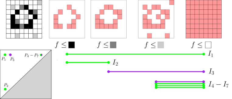
Persistent homology is a technique of TDA coming from topological algebra that allows the user to compute and encode topological information of datasets in a compact descriptor called the persistence diagram. Given a dataset $X$, often given in the form of a point cloud in $\mathbb{R}^{n}$, and a continuous and real-valued function $f:X\rightarrow\mathbb{R}$, the persistence diagram of $f$ can be computed under mild conditions (the function has to be tame, see [CdSGO16] for more details), and consists in a finite set of points with multiplicities in the upper-diagonal half-plane $\mathrm{Dg}(f)=\{(x_{i},y_{i})\}\subset\{(x,y)\in\mathbb{R}^{2}:y>x\}$. This set of points is computed from the family of sublevel sets of $f$, that is the sets of the form $f^{-1}((-\infty,\alpha])$, for some $\alpha\in\mathbb{R}$. More precisely, persistence diagrams encode the different topological events that occur as $\alpha$ increases from $-\infty$ to $+\infty$. Such topological events include creation and merging of connected components and cycles in every dimension; see Figure 1. Intuitively, persistent homology records, for each topological feature that appears in the family of sublevel sets, the value $\alpha_{b}$ at which the feature appears, called the birth value, and the value $\alpha_{d}$ at which it gets merged or filled in, called the death value. These values are then used as coordinates for a corresponding point in the persistence diagram. Note that several features may have the same birth and death values, so points in the persistence diagram have multiplicities. Moreover, since $\alpha_{d}\geq\alpha_{b}$, these points are always located above the diagonal $\Delta=\{(x,x):x\in\mathbb{R}\}$. A general intuition about persistence diagrams is that the distance of a point to $\Delta$ is a direct measure of its relevance: if a point is close to $\Delta$, it means that the corresponding cycle got filled in right after its appearance, thus suggesting that it is likely due to noise in the dataset. On the contrary, points that are far away from $\Delta$ represent cycles with a significant life span, and are more likely to be relevant for the analysis. We refer the interested reader to [EH10, Oud15] for more details about persistent homology.

Figure 1: Example of persistence diagram computation. The space we consider is a blurry image of a zero, and the function $f$ that we use is the grey level value on each pixel. We show four different sublevel sets of $f$. For each sublevel set, the corresponding pixels are displayed in pink color. In the first sublevel set, two connected components are present in the sublevel set, so we start two intervals $I_{1}$ and $I_{2}$. In the second one, one connected component got merged to the other, so we stop the corresponding interval $I_{2}$, and a cycle (loop) is created, so we start a third interval $I_{3}$. In the third sublevel set, a new small cycle is created, as well as three more connected components. In the fourth sublevel set, all pixels belong to the set: all cycles are filled in and all connected components are merged together, so we stop all intervals. Finally, each interval $I_{k}$ is represented as a point $P_{k}$ in the plane (using the endpoints as coordinates).

Notation.

Let ${\mathcal{D}}$ be the space of persistence diagrams with countable number of points. More formally, ${\mathcal{D}}$ can be equivalently defined as a functional space $\{m:\mathbb{R}^{2}\setminus\Delta\rightarrow\mathbb{N}\,:\,{\rm supp}(m)\text{ is countable}\}$, where each point $q\in{\rm supp}(m)$ is a point in the corresponding persistence diagram with multiplicity $m(q)$. Let ${\mathcal{D}}_{N}$ be the space of persistence diagrams with less than $N$ points, i.e., ${\mathcal{D}}_{N}=\{m:\mathbb{R}^{2}\setminus\Delta\rightarrow\mathbb{N}\,:\,\sum_{q}m(q)<N\}$. Let ${\mathcal{D}}^{L}$ be the space of persistence diagrams included in $[-L,L]^{2}$, i.e., ${\mathcal{D}}^{L}=\{m:\mathbb{R}^{2}\setminus\Delta\rightarrow\mathbb{N}\,:\,{\rm supp}(m)\subset[-L,L]^{2}\}$. Finally, let ${\mathcal{D}}_{N}^{L}$ be the space of persistence diagrams with less than $N$ points included in $[-L,L]^{2}$, i.e., ${\mathcal{D}}_{N}^{L}={\mathcal{D}}_{N}\cap{\mathcal{D}}^{L}$. Obviously, we have the following sequences of (strict) inclusions: ${\mathcal{D}}_{N}^{L}\subset{\mathcal{D}}_{N}\subset{\mathcal{D}}$, and ${\mathcal{D}}_{N}^{L}\subset{\mathcal{D}}^{L}\subset{\mathcal{D}}$.

Diagram distances.

Persistence diagrams can be efficiently compared using the diagram distances, which is a family of distances parametrized by an integer $p$ that rely on the computation of partial matchings. Recall that two persistence diagrams $\mathrm{Dg}_{1}$ and $\mathrm{Dg}_{2}$ may have different number of points. A partial matching $\Gamma$ between $\mathrm{Dg}_{1}$ and $\mathrm{Dg}_{2}$ is a subset of $\mathrm{Dg}_{1}\times\mathrm{Dg}_{2}$. It comes along with $\Gamma_{1}$ (resp. $\Gamma_{2}$), which is the set of points of $\mathrm{Dg}_{1}$ (resp. $\mathrm{Dg}_{2}$) that are not matched to a point of $\mathrm{Dg}_{2}$ (resp. $\mathrm{Dg}_{1}$) by $\Gamma$. The $p$-cost of $\Gamma$ is given as:

$$c_{p}(\Gamma)=\sum_{(p,q)\in\Gamma}\|p-q\|_{\infty}^{p}+\sum_{p\in\Gamma_{1}}\|p-\Delta\|_{\infty}^{p}+\sum_{q\in\Gamma_{2}}\|q-\Delta\|_{\infty}^{p}.$$

The $p$-diagram distance is then defined as the cost of the best partial matching:

Definition 2.1.

Given two persistence diagrams $\mathrm{Dg}_{1}$ and $\mathrm{Dg}_{2}$, the $p$-diagram distance $d_{p}$ is defined as:

$$d_{p}(\mathrm{Dg}_{1},\mathrm{Dg}_{2})={\rm inf}_{\Gamma}\ \sqrt[p]{c_{p}(\Gamma)}.$$

Note that in the literature, these distances are often called the Wasserstein distances between persistence diagrams. Here, we follow the denomination of [CCO17]. In particular, taking a maximum instead of a sum in the definition of the cost,

$$c_{\infty}(\Gamma)=\max_{(p,q)\in\Gamma}\|p-q\|_{\infty}+\max_{p\in\Gamma_{1}}\|p-\Delta\|_{\infty}+\max_{q\in\Gamma_{2}}\|q-\Delta\|_{\infty}.$$

allows to add one more distance in the family, the bottleneck distance $d_{\infty}(\mathrm{Dg}_{1},\mathrm{Dg}_{2})={\rm inf}_{\Gamma}\ c_{\infty}(\Gamma)$.

Stability.

A useful property of persistence diagrams is stability. Indeed, it is well known in the literature that persistence diagrams computed from close functions are close themselves in the bottleneck distance:

Theorem 2.2 ([CSEH07, CdSGO16]).

Given two tame functions $f,g:X\rightarrow\mathbb{R}$, one has the following inequality:

$$d_{\infty}(\mathrm{Dg}(f),\mathrm{Dg}(g))\leq\|f-g\|_{\infty}.$$ (1)

In other words, the map $\mathrm{Dg}$ is 1-Lipschitz. Note that stability results exist as well for the other diagram distances, but these results are weaker than the above Lipschitz condition, and they require more conditions—see [Oud15].

2.2 Bi-Lipschitz embeddings.

The main question that we adress in this article is the one of preserving the persistence diagram metric properties when using embeddings into Hilbert spaces. For instance, one may ask the images of persistence diagrams under a feature map into a Hilbert space to be stable as well. A natural question is then whether a lower bound also holds, i.e., whether the feature map $\Phi$ is a bi-Lipschitz embedding between $({\mathcal{D}},d_{p})$ and $\mathcal{H}$.

Definition 2.3.

Let $(X,d_{X})$ and $(Y,d_{Y})$ be two metric spaces. A bi-Lipschitz embedding between $(X,d_{X})$ and $(Y,d_{Y})$ is a map $\Phi:X\rightarrow Y$ such that there exist constants $0<A,B<\infty$ such that:

$$A\,d_{X}(x,x^{\prime})\leq d_{Y}(\Phi(x),\Phi(x^{\prime}))\leq B\,d_{X}(x,x^{\prime}),$$

for any $x,x^{\prime}\in X$. The metrics $d_{X}$ and $d_{Y}$ are called strongly equivalent, and the constants $A$ and $B$ are called the lower and upper metric distortion bounds respectively. If $A=B=1$, $\Phi$ is called an isometric embedding.

Note that this definition is equivalent to the commonly used definition that additionally requires $A=\frac{1}{B}$.

Remark 2.4.

Finding an isometric embedding of persistence diagrams into a Hilbert space is impossible since geodesics are unique in a Hilbert space while this is not the case for persistence diagrams, as shown in the proof of Proposition 2.4 in [TMMH14].

Remark 2.5.

For feature maps that are bounded, i.e., those maps $\Phi$ such that there exists a constant $C>0$ for which $\|\Phi(\mathrm{Dg})\|\leq C$ for all $\mathrm{Dg}$, it is obviously impossible to find a bi-Lipschitz embedding. This involves for instance the Sliced Wasserstein (SW) feature map [CCO17], which is defined implicitly from a Gaussian-like function. However, note that if the SW feature map is restricted to a set of persistence diagrams which are close to each other with respect to the SW distance, then the distance in the Hilbert space corresponding to the SW feature map is actually equivalent to the square root of the SW distance. Hence, we added the square root of the SW distance in our experiment in Section 5.

3 Mapping into separable Hilbert spaces

In our first main result, we use separability to determine whether a bi-Lipschitz embedding can exist between the space of persistence diagrams and a Hilbert space.

Definition 3.1.

A metric space is called separable if it has a dense countable subset.

For instance, the following three Hilbert spaces (equipped with their canonical metrics) are separable: $\mathbb{R}^{n}$, $\ell_{2}$ and $L_{2}(\Omega)$, where $\Omega$ is separable. The two following results describe well-known properties of separable spaces.

Proposition 3.2.

Any subspace of a separable metric space is separable as well.

Proposition 3.3.

Let $(X,d_{X})$ and $(Y,d_{Y})$ be two metric spaces, and assume there is a bi-Lipschitz embedding $\Phi:X\rightarrow Y$, with Lipschitz constants $A$ and $B$. Then $X$ is separable if and only if ${\rm im}(\Phi)$ is separable.

The following lemma shows that for a feature map $\Phi$ which is bi-Lipschitz when restricted to ${\mathcal{D}}_{N}^{L}$, the limits of the corresponding constants can actually be used to study the general metric distortion in ${\mathcal{D}}$.

Lemma 3.4.

Let $p\in\mathbb{N}^{*}$ and let $d$ be a metric on persistence diagrams such that $d$ is continuous with respect to $d_{p}$ on ${\mathcal{D}}$. Let

$$R_{N}^{L} =\left\{\frac{d_{p}(\mathrm{Dg},\mathrm{Dg}^{\prime})}{d(\mathrm{Dg},\mathrm{Dg}^{\prime})}:\mathrm{Dg}\neq\mathrm{Dg}^{\prime}\in{\mathcal{D}}_{N}^{L}\right\},$$

$$A_{N}^{L} =\inf\ R_{N}^{L}\quad\text{and}\quad B_{N}^{L}=\sup\ R_{N}^{L}.$$

Since $A_{N}^{L}$ is nonincreasing and $B_{N}^{L}$ is nonincreasing with respect to $N$ and $L$, we define:

$$A_{N} =\liminf_{L\to\infty}A_{N}^{L},\ \ A^{L}=\liminf_{N\to\infty}A_{N}^{L},\ \ A=\liminf_{N,L\to\infty}A_{N}^{L}.$$

$$B_{N} =\limsup_{L\to\infty}B_{N}^{L},\ \ B^{L}=\limsup_{N\to\infty}B_{N}^{L},\ \ B=\limsup_{N,L\to\infty}B_{N}^{L}.$$

We define $B_{N}$, $B^{L}$, $B$ similarly, since $B_{N}^{L}$ is nondecreasing with respect to $N$ and $L$. Then the following inequalities hold:

$$A^{L}\,d(\mathrm{Dg},\mathrm{Dg}^{\prime})\leq\, d_{p}(\mathrm{Dg},\mathrm{Dg}^{\prime})\leq B^{L}\,d(\mathrm{Dg},\mathrm{Dg}^{\prime}) \text{ for all }\mathrm{Dg},\mathrm{Dg}^{\prime} \in{\mathcal{D}}^{L},$$

$$A_{N}\,d(\mathrm{Dg},\mathrm{Dg}^{\prime})\leq\, d_{p}(\mathrm{Dg},\mathrm{Dg}^{\prime})\leq B_{N}\,d(\mathrm{Dg},\mathrm{Dg}^{\prime}) \text{ for all }\mathrm{Dg},\mathrm{Dg}^{\prime} \in{\mathcal{D}}_{N},$$

$$A\,d(\mathrm{Dg},\mathrm{Dg}^{\prime})\leq\, d_{p}(\mathrm{Dg},\mathrm{Dg}^{\prime})\leq B\,d(\mathrm{Dg},\mathrm{Dg}^{\prime}) \text{ for all }\mathrm{Dg},\mathrm{Dg}^{\prime} \in{\mathcal{D}}.$$

Note that $A$, $A_{N}$, $A^{L}$, $B$, $B_{N}$ and $B^{L}$ may be equal to $0$ or $+\infty$, so it does not necessarily hold that $d$ and $d_{p}$ are strongly equivalent on ${\mathcal{D}}_{N}$, ${\mathcal{D}}^{L}$ or ${\mathcal{D}}$.

Proof.

We only prove the last inequality, since the proof extends verbatim to the other two. Pick any two persistence diagrams $\mathrm{Dg},\mathrm{Dg}^{\prime}\in{\mathcal{D}}$. Let $\Gamma=\{(p_{i},q_{i})\}_{i\in\mathbb{N}}$ be an optimal partial matching achieving $d_{p}(\mathrm{Dg},\mathrm{Dg}^{\prime})$, where $p_{i}$ (resp. $q_{i}$) is either in $\mathrm{Dg}$ (resp. $\mathrm{Dg}^{\prime}$) or in $\pi_{\Delta}(\mathrm{Dg}^{\prime})$ (resp. $\pi_{\Delta}(\mathrm{Dg})$). Given $n\in\mathbb{N}$, we define two sequences of persistence diagrams $\{\mathrm{Dg}_{n}\}_{n\in\mathbb{N}}$ and $\{\mathrm{Dg}^{\prime}_{n}\}_{n\in\mathbb{N}}$ recursively with $\mathrm{Dg}_{0}=\mathrm{Dg}^{\prime}_{0}=\emptyset$ and:

$$\mathrm{Dg}_{n+1} =\begin{cases}\mathrm{Dg}_{n}&\text{if }p_{n+1}\in\pi_{\Delta}(\mathrm{Dg}^{\prime}),\\ \mathrm{Dg}_{n}\cup\{p_{n+1}\}&\text{otherwise,}\end{cases}$$

$$\mathrm{Dg}^{\prime}_{n+1} =\begin{cases}\mathrm{Dg}^{\prime}_{n}&\text{if }q_{n+1}\in\pi_{\Delta}(\mathrm{Dg}),\\ \mathrm{Dg}^{\prime}_{n}\cup\{q_{n+1}\}&\text{otherwise.}\end{cases}$$

Let us define

$$l_{n} =\max\{\max\{\|p\|_{\infty}:p\in\mathrm{Dg}_{n}\},\max\{\|q\|_{\infty}:q\in\mathrm{Dg}^{\prime}_{n}\}\},$$

$$s_{n} =\max\{{\rm card}(\mathrm{Dg}_{n}),{\rm card}(\mathrm{Dg}^{\prime}_{n})\},$$

Note that both $\{l_{n}\}_{n\in\mathbb{N}}$ and $\{s_{n}\}_{n\in\mathbb{N}}$ are nondecreasing. We have $\mathrm{Dg}_{n},\mathrm{Dg}^{\prime}_{n}\in\mathcal{D}_{s_{n}}^{l_{n}}$ and thus:

$$A_{s_{n}}^{l_{n}}\,d(\mathrm{Dg}_{n},\mathrm{Dg}^{\prime}_{n})\leq d_{p}(\mathrm{Dg}_{n},\mathrm{Dg}^{\prime}_{n})\leq B_{s_{n}}^{l_{n}}\,d(\mathrm{Dg}_{n},\mathrm{Dg}^{\prime}_{n}).$$ (2)

Assuming $d_{p}(\mathrm{Dg}_{n},\mathrm{Dg}^{\prime}_{n})\rightarrow d_{p}(\mathrm{Dg},\mathrm{Dg}^{\prime})$ , it follows that $d(\mathrm{Dg}_{n},\mathrm{Dg}^{\prime}_{n})\rightarrow d(\mathrm{Dg},\mathrm{Dg}^{\prime})$ by continuity of $d$. We finally obtain the desired inequality by letting $n\rightarrow+\infty$ in (2). ∎

A corollary of the previous results is that even if a feature map taking values in a separable Hilbert space might be bi-Lipschitz when restricted to ${\mathcal{D}}_{N}^{L}$, the corresponding bounds have to go to 0 or $+\infty$ as soon as the domain of the feature map is not separable.

Theorem 3.5.

Let $\Phi:\mathcal{D}_{\Phi}\rightarrow\mathcal{H}$ be a feature map defined on a non-separable subspace $\mathcal{D}_{\Phi}$ of persistence diagrams containing every ${\mathcal{D}}_{N}^{L}$, i.e., ${\mathcal{D}}_{N}^{L}\subset\mathcal{D}_{\Phi}$ for each $N,L$. Assume $\Phi$ takes values in a separable Hilbert space $\mathcal{H}$, and that $\Phi$ is bi-Lipschitz on each ${\mathcal{D}}_{N}^{L}$ with constants $A_{N}^{L},B_{N}^{L}$. Then either $A_{N}^{L}\rightarrow 0$ or $B_{N}^{L}\rightarrow+\infty$ when $N,L\rightarrow+\infty$.

Many feature maps defined in the literature, such as the Persistence Weighted Gaussian feature map [KFH18] or the Landscape feature map [Bub15], actually take value in the separable function space $L^{2}(\Omega)$, where $\Omega$ is the upper half-plane $\{(x,y)\,:\,x\leq y\}$. Hence, to illustrate how Theorem 3.5 applies to these feature maps, we now provide two lemmata. In the first one, we define a set $\mathcal{S}$ which is not separable with respect to $d_{1}$, and in the second one, we show that $\mathcal{S}$ is actually included in the domain $\mathcal{D}_{\Phi}$ of these feature maps.

Lemma 3.6.

Consider the sequence of points $\{p_{k}=(k,k+\frac{1}{k})\,:\,k\in\mathbb{N}\}$, and define the set $\mathcal{S}=\{\mathrm{Dg}_{u}\}_{u\in\mathcal{U}}\subset{\mathcal{D}}$, where $\mathcal{U}$ is the set of sequences with values in $\{0,1\}$, with: $\mathrm{Dg}_{u}=\{p_{i}\,:\,i\in{\rm supp}(u)\}$. Then $(\mathcal{S},d_{1})$ is not separable.

Proof.

First note that since the sequences $u\in\mathcal{U}$ can have infinite support, the spaces $\mathcal{U}$ and $\mathcal{S}=\{\mathrm{Dg}_{u}\}_{u\in\mathcal{U}}$ are not countable.

Let $\sim$ be the equivalence relation on $\mathcal{S}$ defined with:

$$\mathrm{Dg}_{u}\sim\mathrm{Dg}_{v}\Longleftrightarrow{\rm supp}(u)\ \triangle\ {\rm supp}(v)<+\infty,$$

where $\triangle$ denotes the symmetric difference of sets. Since the set of sequences with finite support is countable, it follows that each equivalence class $[\mathrm{Dg}_{u}]_{\sim}$ is countable as well. In particular, this means that the set of equivalence classes $\mathcal{S}/\sim$ is uncountable, since otherwise $\mathcal{S}$ would be countable as a countable union of countable equivalence classes.

We now prove the result by contradiction. Assume that $\mathcal{S}$ is separable, and let $\mathcal{S}^{\prime}\subset\mathcal{S}$ be the corresponding dense countable subset of $\mathcal{S}$. Let $\epsilon>0$. Then for each $u\in\mathcal{U}$, there is at least one sequence $u^{\prime}\in\mathcal{U}$ such that $\mathrm{Dg}_{u^{\prime}}\in\mathcal{S}^{\prime}$ and $d_{1}(\mathrm{Dg}_{u},\mathrm{Dg}_{u^{\prime}})\leq\epsilon$. We now claim that every such $u^{\prime}$ satisfies $\mathrm{Dg}_{u^{\prime}}\in[\mathrm{Dg}_{u}]_{\sim}$. Indeed, assume $\mathrm{Dg}_{u^{\prime}}\not\in[\mathrm{Dg}_{u}]_{\sim}$ and let ${\mathcal{I}}={\rm supp}(u^{\prime})\ \triangle\ {\rm supp}(u)$. Then, since $|\mathcal{I}|=+\infty$, we would have

$$d_{1}(\mathrm{Dg}_{u},\mathrm{Dg}_{u^{\prime}})=\sum_{i\in\mathcal{I}}\frac{1}{i}=+\infty>\epsilon,$$

which is not possible. Hence, this means that $|\mathcal{S}^{\prime}|\geq|\mathcal{S}/\sim|$. However, we showed that $\mathcal{S}/\sim$ is uncountable, meaning that $\mathcal{S}^{\prime}$ is uncountable as well, which leads to a contradiction since $\mathcal{S}^{\prime}$ is countable by assumption. ∎

We now show that the Persistence Weighted Gaussian and the Landscape feature maps are well-defined on the set $\mathcal{S}$. Let us first formally define these feature maps.

Definition 3.7.

Given $p=(u,v)\in\mathbb{R}^{2}$, $u\leq v$, let $\phi_{p}$ be the triangular function defined with $\phi_{p}(t)=\frac{v-u}{2}(1-\frac{2}{v-u}|t-\frac{u+v}{2}|)$ if $x\leq t\leq y$ and 0 otherwise. Then, given a persistence diagram $\mathrm{Dg}$, let $\lambda_{k}:t\mapsto{\rm kmax}\{\phi_{p}(t)\}_{p\in\mathrm{Dg}}$, where kmax denotes the $k$-th largest element. The Landscape feature map is defined as:

$$\Phi_{\rm L}:\mathrm{Dg}\mapsto\bar{\lambda},\quad\text{where}\quad\bar{\lambda}(x,y)=\begin{cases}\lambda_{\lceil x\rceil}(y)&x\geq 0,\\ 0&\text{otherwise}.\end{cases}$$

Definition 3.8.

Let $\omega:\mathbb{R}^{2}\rightarrow\mathbb{R}$ be a weight function and $\sigma>0$. The Persistence Weighted Gaussian feature map is defined as:

$$\Phi^{\omega}_{\rm PWG}:\mathrm{Dg}\mapsto\sum_{p\in\mathrm{Dg}}\omega(p){\rm e}^{-\frac{\|\cdot-p\|_{2}^{2}}{2\sigma^{2}}}.$$

Proposition 3.9.

Let $(x,y)\mapsto(y-x)^{2}$ be the weight function $(x,y)\mapsto(y-x)^{2}$. Let $\mathcal{S}$ be the set of persistence diagrams defined in Lemma 3.6. Then:

$$\mathcal{S}\subset\mathcal{D}_{\Phi^{\omega}_{\rm PWG}}\text{ and }\mathcal{S}\subset\mathcal{D}_{\Phi_{\rm L}}.$$

Proof.

Let $u_{k}\in\mathcal{U}$ be the sequence defined with $u_{n}=1$ if $n\leq k$ and $u_{n}=0$ otherwise. To show the desired result, it suffices to show that $\{\Phi^{\omega}_{\rm PWG}(\mathrm{Dg}_{u_{k}})\}_{k\in\mathbb{N}}$ and $\{\Phi_{\rm L}(\mathrm{Dg}_{u_{k}})\}_{k\in\mathbb{N}}$ are Cauchy sequences in $L^{2}(\mathbb{R}^{2})$. Let $q\geq p\geq 1$, and let us study $\|\Phi(\mathrm{Dg}_{u_{q}})-\Phi(\mathrm{Dg}_{u_{p}})\|^{2}_{L^{2}(\mathbb{R}^{2})}$ for each feature map.

• Case $\Phi^{\omega}_{\rm PWG}$. We have the following inequalities:

  $$\|\Phi^{\omega}_{\rm PWG} (\mathrm{Dg}_{u_{q}})-\Phi^{\omega}_{\rm PWG}(\mathrm{Dg}_{u_{p}})\|^{2}_{L^{2}(\mathbb{R}^{2})}$$

  $$=\int_{\mathbb{R}^{2}}\left(\sum_{k=p}^{q}\frac{1}{k^{2}}{\rm e}^{-\frac{\|x-p_{k}\|^{2}_{2}}{2\sigma^{2}}}\right)^{2}{\rm d}x=\sum_{k=p}^{q}\sum_{l=p}^{q}\frac{1}{k^{2}l^{2}}\int_{\mathbb{R}^{2}}{\rm e}^{-\frac{\|x-p_{k}\|^{2}_{2}+\|x-p_{l}\|^{2}_{2}}{2\sigma^{2}}}{\rm d}x$$

  $$=\pi\sigma^{2}\sum_{k=p}^{q}\sum_{l=p}^{q}\frac{1}{k^{2}l^{2}}{\rm e}^{-\frac{\|p_{k}-p_{l}\|^{2}_{2}}{4\sigma^{2}}}\text{ (cf Appendix C in~{}\cite[cite]{[\@@bibref{}{Reininghaus14}{}{}]} for a proof of this equality)}$$

  $$\leq\pi\sigma^{2}\left(\sum_{k=p}^{q}\frac{1}{k^{2}}\right)\left(\sum_{l=p}^{q}\frac{1}{l^{2}}\right)$$

  The result simply follows from the fact that $\{\sum_{k=1}^{n}\frac{1}{k^{2}}\}_{n\in\mathbb{N}}$ is convergent and Cauchy.

• Case $\Phi_{\rm L}$. Since all triangular functions, as defined in Definition 3.7, have disjoint support, it follows that the only non-zero lambda function is $\lambda_{1}=\sum_{n=1}^{k}\phi_{n}$, where $\phi_{n}$ is a triangular function defined with $\phi_{n}(t)=\frac{1}{2n}(1-|2n(t-(n+\frac{1}{2n}))|)$ if $n\leq t\leq n+\frac{1}{n}$ and 0 otherwise. See Figure 2.

  

  Figure 2: Image of $\mathrm{Dg}_{u_{4}}$ under $\Phi_{\rm L}$.

  Hence, we have the following inequalities:

  $$\|\Phi_{\rm L} (\mathrm{Dg}_{u_{q}})-\Phi_{\rm L}(\mathrm{Dg}_{u_{p}})\|^{2}_{L^{2}(\mathbb{R}^{2})}$$

  $$=\int_{\mathbb{R}}\left(\sum_{k=p}^{q}\phi_{k}(x)\right)^{2}{\rm d}x=\sum_{k=p}^{q}\sum_{l=p}^{q}\int_{\mathbb{R}}\phi_{k}(x)\phi_{l}(x){\rm d}x$$

  $$=\sum_{k=p}^{q}\int_{\mathbb{R}}\phi_{k}(x)^{2}{\rm d}x\leq\sum_{k=p}^{q}\int_{\mathbb{R}}\phi_{k}(x){\rm d}x=\sum_{k=p}^{q}\frac{1}{4k^{2}}$$

  Again, the result follows from the fact that $\{\sum_{k=1}^{n}\frac{1}{k^{2}}\}_{n\in\mathbb{N}}$ is convergent and Cauchy. ∎

Proposition 3.9 shows that Theorem 3.5 applies (with the metric $d_{1}$ between persistence diagrams) to the Persistence Weighted Gaussian feature map with weight function $(x,y)\mapsto(y-x)^{2}$—actually, any weight function that is equivalent to $(y-x)^{2}$ when $(x,y)$ goes to 0—and the Landscape feature map. In particular, any lower bound for these maps has to go to 0 when $N,L\rightarrow+\infty$ since an upper bound exists for these maps due to their stability properties—see Corollary 15 in [Bub15] and Proposition 3.4 in [KFH18].

4 Mapping into finite-dimensional Hilbert spaces

In our second main result, we show that more can be said about feature maps into $\mathbb{R}^{n}$ (equipped with the Euclidean metric), using the so-called Assouad dimension. This involves all vectorization methods for persistence diagrams that we described in the related work.

Assouad dimension.

The following definition and example are taken from paragraph 10.13 of [Hei01].

Definition 4.1.

Let $(X,d_{X})$ be a metric space. Given a subset $E\subset X$ and $r>0$, let $N_{r}(E)$ be the least number of open balls of radius less than or equal to $r$ that can cover $E$. The Assouad dimension of $X$ is:

$$\operatorname{dim_{A}}(X,d_{X})={\rm inf}\{\alpha>0\,:\,\exists C>0\text{ s.t. }{\rm sup}_{x\in X}N_{\beta r}(B(x,r))\leq C\beta^{-\alpha},\ \forall r>0,\beta\in(0,1]\}.$$

Intuitively, the Assouad dimension measures the number of open balls needed to cover an open ball of larger radius. For example, the Assouad dimension of $\mathbb{R}^{n}$ is $n$. Moreover, the Assouad dimension is preserved by bi-Lipschitz embeddings.

Proposition 4.2 (Lemma 9.6 in [Rob10]).

Let $(X,d_{X})$ and $(Y,d_{Y})$ be metric spaces with a bi-Lipschitz embedding $\Phi:X\rightarrow Y$. Then $\operatorname{dim_{A}}(X,d_{X})=\operatorname{dim_{A}}({\rm im}(\Phi),d_{Y})$.

Non-embeddability.

We now show that ${\mathcal{D}}_{N}^{L}$ cannot be embedded into $\mathbb{R}^{n}$ with bi-Lipschitz embeddings. The proof of this fact is a consequence of the following lemma:

Lemma 4.3.

Let $p\in\mathbb{N}\cup\{\infty\}$, $N\in\mathbb{N}$, and $L>0$. Then $\operatorname{dim_{A}}({\mathcal{D}}_{N}^{L},d_{p})=+\infty$.

Proof.

Let $B_{p}$ denote an open ball with $d_{p}$. We want to show that, for any $\alpha>0$ and $C>0$, it is possible to find a persistence diagram $\mathrm{Dg}\in{\mathcal{D}}_{N}^{L}$, a radius $r>0$ and a factor $\beta\in(0,1]$ such that the number of open balls of radius at most $\beta r$ needed to cover $B_{p}(\mathrm{Dg},r)$ is strictly larger than $C\beta^{-\alpha}$. To this end, we pick arbitrary $\alpha>0$ and $C>0$. The idea of the proof is to define $\mathrm{Dg}$ as the empty diagram, and to derive a lower bound on the number of balls with radius $\beta r$ needed to cover $B_{p}(\mathrm{Dg},r)$ by considering persistence diagrams with one point evenly distributed on the line $\{(x,x+r):x\in[-L,L]\}$ such that the distance between two consecutive points is $r$ in the $\ell_{\infty}$-distance. Indeed, the pairwise distance between any two such persistence diagrams is sufficiently large so that they must belong to different balls. Then we can control the number of persistence diagrams, and thus the number of balls, by taking $r$ sufficiently small.

More formally, let $M=1+\lfloor C\beta^{-\alpha}\rfloor>C\beta^{-\alpha}$. We want to show that we have at least $M$ balls in the cover, meaning that $|\{\mathrm{Dg}_{i}\}|\geq M$. Let $r=2L/M$ and $\beta=\frac{1}{2}$. We define a cover of $B_{p}(\mathrm{Dg},r)$ with open balls of radius less than $\beta r$ centered on a family $\{\mathrm{Dg}_{i}\}$ as follows:

$$B_{p}(\mathrm{Dg},r)\subseteq\bigcup_{i}B_{p}(\mathrm{Dg}_{i},\beta r).$$ (3)

We now define particular persistence diagrams which all lie in different elements of the cover (3). For any $0\leq j\leq M-1$, we let $\mathrm{Dg}^{\prime}_{j}$ denote the persistence diagram containing only the point $(-L+jr,-L+(j+1)r)$. It is clear that each $\mathrm{Dg}^{\prime}_{j}$ is in ${\mathcal{D}}_{N}^{L}$. See Figure 3.

Figure 3: Persistence diagram used in the proof of Lemma 4.3. In this particular example, we have $M=5$.

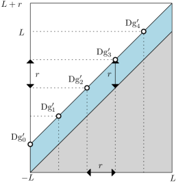
Moreover, since $d_{p}(\mathrm{Dg},\mathrm{Dg}^{\prime}_{j})=\frac{r}{2}<r$, it also follows that $\mathrm{Dg}^{\prime}_{j}\in B_{p}(\mathrm{Dg},r)$.

Hence, according to (3), for each $j$ there exists an integer $i_{j}$ such that $\mathrm{Dg}^{\prime}_{j}\in B_{p}(\mathrm{Dg}_{i_{j}},\beta r)$. Finally, note that $j\neq j^{\prime}\Rightarrow i_{j}\neq i_{j^{\prime}}$. Indeed, assuming that there are $j\neq j^{\prime}$ such that $i_{j}=i_{j^{\prime}}$, and since the distance between $\mathrm{Dg}^{\prime}_{j}$ and $\mathrm{Dg}^{\prime}_{j^{\prime}}$ is always obtained by matching their points to the diagonal, we reach a contradiction with the following application of the triangle inequality:

$$d_{p}(\mathrm{Dg}^{\prime}_{j},\mathrm{Dg}^{\prime}_{j^{\prime}})=2^{\frac{1}{p}}\frac{r}{2}\leq d_{p}(\mathrm{Dg}^{\prime}_{j},\mathrm{Dg}_{i_{j}})+d_{p}(\mathrm{Dg}_{i_{j}},\mathrm{Dg}_{i_{j^{\prime}}})+d_{p}(\mathrm{Dg}_{i_{j^{\prime}}},\mathrm{Dg}^{\prime}_{j^{\prime}})<2\beta r=r.$$

This observation shows that there are at least $M$ different open balls in the cover (3), which concludes the proof. ∎

The following theorem is then a simple consequence of Lemma 4.3 and Proposition 4.2:

Theorem 4.4.

Let $p\in\mathbb{N}\cup\{\infty\}$ and $n\in\mathbb{N}$. Then, for any $N\in\mathbb{N}$ and $L>0$, there is no bi-Lipschitz embedding between $({\mathcal{D}}_{N}^{L},d_{p})$ and $\mathbb{R}^{n}$.

Interestingly, the integers $N$ and $n$ are independent in Theorem 4.4: even if one restricts to persistence diagrams with only one point, it is still impossible to find a bi-Lipschitz embedding into $\mathbb{R}^{n}$, whatever $n$ is.

5 Experiments

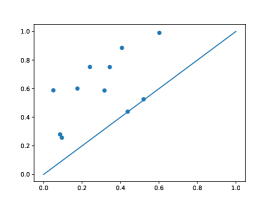
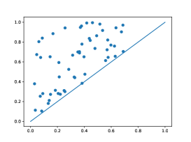
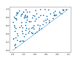
In this section, we illustrate our main results by computing the lower metric distortion bounds for the main stable feature maps in the literature. We use persistence diagrams with increasing number of points to experimentally observe the convergence of this bound to 0, as described in Theorem 3.5. More precisely, we generate 100 persistence diagrams for each cardinality in a range going from 10 to 1000 by uniformly sampling points in the unit upper half-square $\{(x,y)\,:\,0\leq x,y\leq 1,x\leq y\}$. See Figure 4 for an illustration.

Figure 4: Example of synthetic persistence diagrams with cardinalities 10 (left), 60 (middle), and 100 (right) generated for the experiment.

Then, we consider the following feature maps:

• the Persistence Weighted Gaussian with unit bandwidth (PWG) [KFH18],

• the Persistence Scale Space with unit bandwidth (PSS) [RHBK15],

• the Landscape (LS) [Bub15],

• the Persistence Image with resolution $10\times 10$ and unit bandwidth (IM) [AEK⁺17]

• the Topological Vector with 10 dimensions (TV) [COO15],

Since most of these feature maps enjoy stability properties with respect to the first diagram distance $d_{1}$, we compute the ratios between the metrics in the Hilbert spaces corresponding to these feature maps and $d_{1}$. Moreover, we also look at the ratio induced by the square root of the Sliced Wasserstein distance (SW) [CCO17], as suggested by Remark 2.5. All feature maps were computed with the sklearn-tda library, which uses Hera [KMN17] as backend to compute the first diagram distances $d_{1}$ between pairs of persistence diagrams. These ratios are then displayed as boxplots in Figure 5.

Figure 5: Boxplots of the ratios between distances induced by various feature maps and the first diagram distance $d_{1}$.

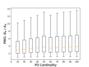
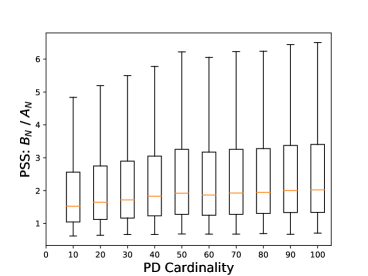
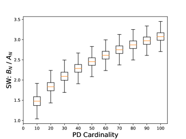
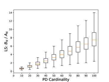
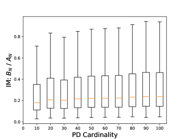
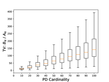
It is clear from Figure 5 that the extreme values of these ratios (the upper tail of the ratio distributions) increase with the cardinality of the persistence diagrams, as expected from Theorem 3.5. This is especially interesting in the case of the Sliced Wasserstein distance since the question whether the lower bound that was proved in [CCO17], which increases with the number of points in the diagrams, was tight or not, i.e., if a lower bound which is oblivious to the number of points could be derived, is still open. Hence, it seems from Figure 5 that this is not the case empirically. It is also interesting to notice that the divergence speed of these ratios differ from a feature map to another. More precisely, it seems like the metric distortion bounds increase linearly with the cardinalities for the TV and LS feature maps and the Sliced Wasserstein distance, while it is increasing at a much lower speed for the other feature maps.

6 Conclusion

In this article, we provided two important theoretical results about the embedding of persistence diagrams in separable Hilbert spaces, which is a common technique in TDA to feed machine learning algorithms with persistence diagrams. Indeed, most of the recent attempts have defined feature maps for persistence diagrams into Hilbert spaces and showed these maps were stable with respect to the first diagram distance, and conjectured whether a lower bound holds as well or not. In this work, we proved that this is never the case if the Hilbert space is finite dimensional, and that such a lower bound has to go to zero with the number of points for most other feature maps in the literature. We also provided experiments that confirm this result, by showing a clear increase of the metric distortion with the number of points for persistence diagrams generated uniformly in the unit upper half-square.

References

- [AEK+17] Henry Adams, Tegan Emerson, Michael Kirby, Rachel Neville, Chris Peterson, Patrick Shipman, Sofya Chepushtanova, Eric Hanson, Francis Motta, and Lori Ziegelmeier. Persistence Images: A Stable Vector Representation of Persistent Homology. Journal of Machine Learning Research, 18(8):1–35, 2017.
- [BL15] Ulrich Bauer and Michael Lesnick. Induced matchings and the algebraic stability of persistence barcodes. Journal of Computational Geometry, 6(2):162–191, 2015.
- [Bub15] Peter Bubenik. Statistical Topological Data Analysis using Persistence Landscapes. Journal of Machine Learning Research, 16:77–102, 2015.
- [Car09] Gunnar Carlsson. Topology and data. Bulletin of the American Mathematical Society, 46:255–308, 2009.
- [CCO17] Mathieu Carrière, Marco Cuturi, and Steve Oudot. Sliced Wasserstein Kernel for Persistence Diagrams. In Proceedings of the 34th International Conference on Machine Learning, 2017.
- [CdSGO16] Frédéric Chazal, Vin de Silva, Marc Glisse, and Steve Oudot. The Structure and Stability of Persistence Modules. Springer, 2016.
- [COO15] Mathieu Carrière, Steve Oudot, and Maks Ovsjanikov. Stable Topological Signatures for Points on 3D Shapes. Computer Graphics Forum, 34, 2015.
- [CSEH07] David Cohen-Steiner, Herbert Edelsbrunner, and John Harer. Stability of Persistence Diagrams. Discrete and Computational Geometry, 37(1):103–120, 2007.
- [DFF15] Barbara Di Fabio and Massimo Ferri. Comparing persistence diagrams through complex vectors. In Image Analysis and Processing — ICIAP 2015, pages 294–305, 2015.
- [EH10] Herbert Edelsbrunner and John Harer. Computational Topology: an introduction. AMS Bookstore, 2010.
- [Hei01] Juha Heinonen. Lectures on Analysis on Metric Spaces. Springer, 2001.
- [HKNU17] Christoph Hofer, Roland Kwitt, Marc Niethammer, and Andreas Uhl. Deep Learning with Topological Signatures. In Advances in Neural Information Processing Systems 30, pages 1633–1643. Curran Associates, Inc., 2017.
- [Kal18] Sara Kališnik. Tropical coordinates on the space of persistence barcodes. Foundations of Computational Mathematics, 2018.
- [KFH16] Genki Kusano, Kenji Fukumizu, and Yasuaki Hiraoka. Persistence Weighted Gaussian Kernel for Topological Data Analysis. In Proceedings of the 33rd International Conference on Machine Learning, pages 2004–2013, 2016.
- [KFH18] Genki Kusano, Kenji Fukumizu, and Yasuaki Hiraoka. Kernel method for persistence diagrams via kernel embedding and weight factor. Journal of Machine Learning Research, 18(189):1–41, 2018.
- [KMN17] Michael Kerber, Dmitriy Morozov, and Arnur Nigmetov. Geometry helps to compare persistence diagrams. Journal of Experimental Algorithmics, 22:1.4:1–1.4:20, September 2017.
- [Oud15] Steve Oudot. Persistence Theory: From Quiver Representations to Data Analysis. Number 209 in Mathematical Surveys and Monographs. American Mathematical Society, 2015.
- [RHBK14] Jan Reininghaus, Stefan Huber, Ulrich Bauer, and Roland Kwitt. A Stable Multi-Scale Kernel for Topological Machine Learning. CoRR, abs/1412.6821, 2014.
- [RHBK15] Jan Reininghaus, Stefan Huber, Ulrich Bauer, and Roland Kwitt. A Stable Multi-Scale Kernel for Topological Machine Learning. In IEEE Conference on Computer Vision and Pattern Recognition, 2015.
- [Rob10] James C. Robinson. Dimensions, Embeddings, and Attractors, volume 186 of Cambridge Tracts in Mathematics. Cambridge University Press, 2010.
- [TMMH14] Katharine Turner, Yuriy Mileyko, Sayan Mukherjee, and John Harer. Fréchet Means for Distributions of Persistence Diagrams. Discrete and Computational Geometry, 52(1):44–70, 2014.