PAC-Bayes bounds for stable algorithms with instance-dependent priors

Abstract

PAC-Bayes bounds have been proposed to get risk estimates based on a training sample. In this paper the PAC-Bayes approach is combined with stability of the hypothesis learned by a Hilbert space valued algorithm. The PAC-Bayes setting is used with a Gaussian prior centered at the expected output. Thus a novelty of our paper is using priors defined in terms of the data-generating distribution. Our main result estimates the risk of the randomized algorithm in terms of the hypothesis stability coefficients. We also provide a new bound for the SVM classifier, which is compared to other known bounds experimentally. Ours appears to be the first stability-based bound that evaluates to non-trivial values.

1 Introduction

This paper combines two directions of research: stability of learning algorithms, and PAC-Bayes bounds for algorithms that randomize with a data-dependent distribution. The combination of these ideas enables the development of risk bounds that exploit stability of the learned hypothesis but are independent of the complexity of the hypothesis class. We use the PAC-Bayes setting with ‘priors’ defined in terms of the data-generating distribution, as introduced by Catoni [2007] and developed further e.g. by Lever et al. [2010] and Parrado-Hernández et al. [2012]. Our work can be viewed as deriving specific results for this approach in the case of stable Hilbert space valued algorithms.

The analysis introduced by Bousquet and Elisseeff [2002], which followed and extended Lugosi and Pawlak [1994] and was further developed by Celisse and Guedj [2016], Abou-Moustafa and Szepesvari [2017] and Liu et al. [2017] among others, shows that stability of learning algorithms can be used to give bounds on the generalisation of the learned functions. Their results work by assessing how small changes in the training set affect the resulting classifiers. Intuitively, this is because stable learning should ensure that slightly different training sets give similar solutions.

In this paper we focus on the sensitivity coefficients (see our Definition 1) of the hypothesis learned by a Hilbert space valued algorithm, and provide an analysis leading to a PAC-Bayes bound for randomized classifiers under Gaussian randomization. As a by-product of the stability analysis we derive a concentration inequality for the output of a Hilbert space valued algorithm. Applying it to Support Vector Machines [Shawe-Taylor and Cristianini, 2004, Steinwart and Christmann, 2008] we deduce a concentration bound for the SVM weight vector, and also a PAC-Bayes performance bound for SVM with Gaussian randomization. Experimental results compare our new bound with other stability-based bounds, and with a more standard PAC-Bayes bound.

Our work contributes to a line of research aiming to develop ‘self-bounding algorithms’ (Freund [1998], Langford and Blum [2003]) in the sense that besides producing a predictor the algorithm also creates a performance certificate based on the available data.

2 Main Result(s)

We consider a learning problem where the learner observes pairs $(X_{i},Y_{i})$ of patterns (inputs) $X_{i}$ from the space $\mathcal{X}$ and labels $Y_{i}$ in the space $\mathcal{Y}$. A training set (or sample) is a finite sequence $S_{n}=((X_{1},Y_{1}),\ldots,(X_{n},Y_{n}))$ of such observations. Each pair $(X_{i},Y_{i})$ is a random element of $\mathcal{X}\times\mathcal{Y}$ whose (joint) probability law is $P\in M_{1}(\mathcal{X}\times\mathcal{Y})$. We think of $P$ as the underlying ‘true’ (but unknown) data-generating distribution. Examples are i.i.d. (independent and identically distributed) in the sense that the joint distribution of $S_{n}$ is the $n$-fold product measure $P^{n}=P\otimes\cdots\otimes P$.

A learning algorithm is a function $\operatorname{\mathsf{A}}:\cup_{n}(\mathcal{X}\times\mathcal{Y})^{n}\to\mathcal{Y}^{\mathcal{X}}$ that maps training samples (of any size) to predictor functions. Given $S_{n}$, the algorithm produces a learned hypothesis $\operatorname{\mathsf{A}}({S_{n}}):\mathcal{X}\to\mathcal{Y}$ that will be used to predict the label of unseen input patterns $X\in\mathcal{X}$. Typically $\mathcal{X}\subset\mathbb{R}^{d}$ and $\mathcal{Y}\subset\mathbb{R}$. For instance, $\mathcal{Y}=\{-1,1\}$ for binary classification, and $\mathcal{Y}=\mathbb{R}$ for regression. A loss function $\ell:\mathbb{R}\times\mathcal{Y}\to[0,\infty)$ is used to assess the quality of hypotheses $h:\mathcal{X}\to\mathcal{Y}$. Say if a pair $(X,Y)$ is sampled, then $\ell(h(X),Y)$ quantifies the dissimilarity between the label $h(X)$ predicted by $h$, and the actual label $Y$. We may write $\ell_{h}(X,Y)=\ell(h(X),Y)$ to express the losses (of $h$) as function of the training examples. The (theoretical) risk of hypothesis $h$ under data-generating distribution $P$ is $R(h,P)=\langle{\ell_{h}},{P}\rangle$. It is also called the error of $h$ under $P$. The empirical risk of $h$ on a sample $S_{n}$ is $R(h,P_{n})=\langle{\ell_{h}},{P_{n}}\rangle$ where $P_{n}=\frac{1}{n}\sum_{i=1}^{n}\delta_{(X_{i},Y_{i})}$ is the empirical measure on $\mathcal{X}\times\mathcal{Y}$ associated to the sample. Notice that the risk (empirical or theoretical) is tied to the choice of a loss function. For instance, consider binary classification with the 0-1 loss $\ell_{01}(y^{\prime},y)=\mathbf{1}[y^{\prime}\neq y]$, where $\mathbf{1}[\cdot]$ is an indicator function equal to $1$ when the argument is true and equal to $0$ when the argument is false. In this case the risk is $R_{01}(c,P)=P[c(X)\neq Y]$, i.e. the probability of misclassifying the random example $(X,Y)\sim P$ when using $c$; and the empirical risk is $R_{01}(c,P_{n})=\frac{1}{n}\sum_{i=1}^{n}\mathbf{1}[c(X_{i})\neq Y_{i}]$, i.e. the in-sample proportion of misclassified examples.

Our main theorem concerns Hilbert space valued algorithms, in the sense that its learned hypotheses live in a Hilbert space $\mathcal{H}$. In this case we may use the Hilbert space norm $\lVert w\rVert_{\mathcal{H}}=\sqrt{\langle{w},{w}\rangle_{\mathcal{H}}}$ to measure the difference between the hypotheses learned from two slightly different samples.

To shorten the notation we will write $\mathcal{Z}=\mathcal{X}\times\mathcal{Y}$. A generic element of this space is $z=(x,y)$, the observed examples are $Z_{i}=(X_{i},Y_{i})$ and the sample of size $n$ is $S_{n}=(Z_{1},\ldots,Z_{n})$.

Definition 1.

Consider a learning algorithm $\operatorname{\mathsf{A}}:\cup_{n}\mathcal{Z}^{n}\to\mathcal{H}$ where $\mathcal{H}$ is a separable Hilbert space. We define the hypothesis sensitivity coefficients of $\operatorname{\mathsf{A}}$ as follows:

$$\beta_{n}=\sup_{i\in[n]}\ \sup_{z_{i},z_{i}^{\prime}}\ \lVert\operatorname{\mathsf{A}}(z_{1:i-1},z_{i},z_{i+1:n})-\operatorname{\mathsf{A}}(z_{1:i-1},z_{i}^{\prime},z_{i+1:n})\rVert_{\mathcal{H}}\,.$$

This is close in spirit to what is called “uniform stability” in the literature, except that our definition concerns stability of the learned hypothesis itself (measured by a distance on the hypothesis space), while e.g. Bousquet and Elisseeff [2002] deal with stability of the loss functional. The latter could be called “loss stability” (in terms of “loss sensitivity coefficients”) for the sake of informative names.

Writing $z_{1:n}\approx z^{\prime}_{1:n}$ when these $n$-tuples differ at one entry (at most), an equivalent formulation to the above is $\beta_{n}=\sup_{z_{1:n}\approx z^{\prime}_{1:n}}\ \lVert\operatorname{\mathsf{A}}(z_{1:n})-\operatorname{\mathsf{A}}(z^{\prime}_{1:n})\rVert_{\mathcal{H}}$. In particular, if two samples $S_{n}$ and $S^{\prime}_{n}$ differ only on one example, then $\lVert\operatorname{\mathsf{A}}(S_{n})-\operatorname{\mathsf{A}}(S^{\prime}_{n})\rVert_{\mathcal{H}}\leq\beta_{n}$. Thus our definition implies stability with respect to replacing one example with an independent copy. Alternatively, one could define $\beta_{n}=\operatorname{ess\,sup}_{S_{n}\approx S^{\prime}_{n}}\ \lVert\operatorname{\mathsf{A}}(S_{n})-\operatorname{\mathsf{A}}(S^{\prime}_{n})\rVert_{\mathcal{H}}$, which corresponds to the “uniform argument stability” of Liu et al. [2017]. We avoid the ‘almost-sure’ technicalities by defining our $\beta_{n}$’s as the maximal difference (in norm) with respect to all $n$-tuples $z_{1:n}\approx z^{\prime}_{1:n}$. The extension to sensitivity when changing several examples is natural: $\lVert\operatorname{\mathsf{A}}(z_{1:n})-\operatorname{\mathsf{A}}(z^{\prime}_{1:n})\rVert_{\mathcal{H}}\leq\beta_{n}\sum_{i=1}^{n}\mathbf{1}[z_{i}\neq z^{\prime}_{i}]$. Note that $\beta_{n}$ is a Lipschitz factor with respect to the Hamming distance. The “total Lipschitz stability” of Kontorovich [2014] is a similar notion for stability of the loss functional. The “collective stability” of London et al. [2013] is not comparable to ours (different setting) despite the similar look.

We will consider randomized classifiers that operate as follows. Let $\mathcal{C}$ be the classifier space, and let $Q\in M_{1}(\mathcal{C})$ be a probability distribution over the classifiers. To make a prediction the randomized classifier picks $c\in\mathcal{C}$ according to $Q$ and predicts a label with the chosen $c$. Each prediction is made with a fresh $c$ draw. For simplicity we use the same label $Q$ for the probability distribution and for the corresponding randomized classifier. The risk measures $R(c,P)$ and $R(c,P_{n})$ are extended to randomized classifiers: $R(Q,P)\equiv\int_{\mathcal{C}}R(c,P)\hskip 2.0ptdQ(c)$ is the average theoretical risk of $Q$, and $R(Q,P_{n})\equiv\int_{\mathcal{C}}R(c,P_{n})\hskip 2.0ptdQ(c)$ its average empirical risk. Given two distributions $Q_{0},Q\in M_{1}(\mathcal{C})$, the Kullback-Leibler divergence (a.k.a. relative entropy) of $Q$ with respect to $Q_{0}$ is

$$\vspace{-4mm}\operatorname{\mathit{KL}}(Q\|Q_{0})=\int_{\mathcal{C}}\log\bigl{(}\frac{dQ}{dQ_{0}}\bigr{)}\hskip 2.0ptdQ\,.\vspace{-4mm}$$

Of course this makes sense when $Q$ is absolutely continuous with respect to $Q_{0}$, which ensures that the Radon-Nikodym derivative $dQ/dQ_{0}$ exists. For Bernoulli distributions with parameters $q$ and $q_{0}$ we write $\operatorname{\mathit{KL}}(q\|q_{0})=q\log(\frac{q}{q_{0}})+(1-q)\log(\frac{1-q}{1-q_{0}})$, and $\operatorname{\mathit{KL}}_{+}(q\|q_{0})=\operatorname{\mathit{KL}}(q\|q_{0})\mathbf{1}[q<q_{0}]$.

2.1 A PAC-Bayes bound for stable algorithms with Gaussian randomization

This is our main result:

Theorem 2.

Let $\operatorname{\mathsf{A}}$ be a Hilbert space valued algorithm. Suppose that (once trained) the algorithm will randomize according to Gaussian distributions $Q=\mathcal{N}(\operatorname{\mathsf{A}}(S_{n}),\sigma^{2}I)$. If $\operatorname{\mathsf{A}}$ has hypothesis stability coefficients $\beta_{n}$, then for any randomization variance $\sigma^{2}>0$, for any $\delta\in(0,1)$, with probability $\geq 1-2\delta$ we have

$$\operatorname{\mathit{KL}}_{+}(R(Q,P_{n})\|R(Q,P))\leq\frac{\frac{n\beta_{n}^{2}}{2\sigma^{2}}\left(1+\sqrt{\frac{1}{2}\log\bigl{(}\frac{1}{\delta}\bigr{)}}\ \right)^{2}+\log(\frac{n+1}{\delta})}{n}\,.$$

The proof of our theorem combines stability of the learned hypothesis (in the sense of Definition 1) and a PAC-Bayes bound for the average theoretical error of a randomized classifier, quoted below in Section 4 (Proofs) for reference. Note that the randomizing distribution $Q$ depends on the sample. Literature on the PAC-Bayes framework for learning linear classifiers include Germain et al. [2015] and Parrado-Hernández et al. [2012] with references. Application of the PAC-Bayes framework to training neural networks can be seen e.g. in London [2017], Dziugaite and Roy [2017].

2.2 A PAC-Bayes bound for SVM with Gaussian randomization

For a Support Vector Machine (SVM) with feature map $\varphi:\mathcal{X}\to\mathcal{H}$ into a separable Hilbert space $\mathcal{H}$, we may identify a linear classifier $c_{w}(\cdot)=\operatorname{sign}(\langle w,\varphi(\cdot)\rangle)$ with a vector $w\in\mathcal{H}$. With this identification we can regard an SVM as a Hilbert space valued mapping that based on a training sample $S_{n}$ learns a weight vector $W_{n}=\operatorname{SVM}(S_{n})\in\mathcal{H}$. In this context, stability of the SVM’s solution then reduces to stability of the learned weight vector.

To be specific, let $\operatorname{SVM}_{\lambda}(S_{n})$ be the SVM that regularizes the empirical risk over the sample $S_{n}$ by solving the following optimization problem:

$$\operatorname*{arg\,min}_{w}\biggl{(}\frac{\lambda}{2}\lVert w\rVert^{2}+\frac{1}{n}\sum_{i=1}^{n}\ell(c_{w}(X_{i}),Y_{i})\biggr{)}\,.$$ (svm)

Our stability coefficients in this case satisfy $\beta_{n}\leq\frac{2}{\lambda n}$ (Example 2 of Bousquet and Elisseeff [2002], adapted to our setting). Then a direct application of our Theorem 2 together with a concentration argument for the SVM weight vector (see our Corollary 9 below) gives the following:

Corollary 3.

Let $W_{n}=\operatorname{SVM}_{\lambda}(S_{n})$. Suppose that (once trained) the algorithm will randomize according to Gaussian distributions $Q=\mathcal{N}(W_{n},\sigma^{2}I)$. For any randomization variance $\sigma^{2}>0$, for any $\delta\in(0,1)$, with probability $\geq 1-2\delta$ we have

$$\operatorname{\mathit{KL}}_{+}(R(Q,P_{n})\|R(Q,P))\leq\frac{\frac{2}{\sigma^{2}\lambda^{2}n}\left(1+\sqrt{\frac{1}{2}\log\bigl{(}\frac{1}{\delta}\bigr{)}}\ \right)^{2}+\log(\frac{n+1}{\delta})}{n}\,.$$

In closing this section we mention that our main theorem is general in that it may be specialized to any Hilbert space valued algorithm. This covers any regularized ERM algorithm [Liu et al., 2017]. We applied it to SVM’s whose hypothesis sensitivity coefficients (as in our Definition 1) are known. It can be argued that neural networks (NN’s) fall under this framework as well. Then an appealing future research direction, with deep learning in view, is to figure out the sensitivity coefficients of NN’s trained by Stochastic Gradient Descent. Then our main theorem could be applied to provide non-vacuous bounds for the performance of NN’s, which we believe is very much needed.

3 Comparison to other bounds

For reference we list several risk bounds (including ours). They are in the context of binary classification ($\mathcal{Y}=\{-1,+1\}$). For clarity, risks under the 0-1 loss are denoted by $R_{01}$ and risks with respect to the (clipped) hinge loss are denoted by $R_{\mathrm{hi}}$. Bounds requiring a Lipschitz loss function do not apply to the 0-1 loss. However, the 0-1 loss is upper bounded by the hinge loss, allowing us to upper bound the risk with respect to the former in therms of the risk with respect to the latter. On the other hand, results requiring a bounded loss function do not apply to the regular hinge loss. In those cases the clipped hinge loss is used, which enjoys boundedness and Lipschitz continuity.

3.1 P@EW: Our new instance-dependent PAC-Bayes bound

Our Corollary 3, with $Q=\mathcal{N}(W_{n},\sigma^{2}I)$, a Gaussian centered at $W_{n}=\operatorname{SVM}_{\lambda}(S_{n})$ with randomization variance $\sigma^{2}$, gives the following risk bound which holds with probability $\geq 1-2\delta$:

$$\operatorname{\mathit{KL}}_{+} (R_{01}(Q,P_{n})\|R_{01}(Q,P))\leq\frac{2}{\sigma^{2}\lambda^{2}n^{2}}\biggl{(}1+\sqrt{\frac{1}{2}\log\bigl{(}\frac{1}{\delta}\bigr{)}}\ \biggr{)}^{2}+\frac{1}{n}\log\bigl{(}\frac{n+1}{\delta}\bigr{)}\,.$$

As will be clear from the proof (see Section 4 below), this bound is obtained from the PAC-Bayes bound (Theorem 4) using a prior centered at the expected weight.

3.2 P@O: Prior at the origin PAC-Bayes bound

The PAC-Bayes bound Theorem 4 again with $Q=\mathcal{N}(W_{n},\sigma^{2}I)$, gives the following risk bound which holds with probability $\geq 1-\delta$:

$$\forall\sigma^{2},\hskip 8.53581pt\operatorname{\mathit{KL}}_{+}(R_{01}(Q,P_{n})\|R_{01}(Q,P))\leq\frac{1}{2\sigma^{2}n}\lVert W_{n}\rVert^{2}+\frac{1}{n}\log\bigl{(}\frac{n+1}{\delta}\bigr{)}\,.$$

3.3 Bound of Liu et al. [2017]

From Corollary 1 of Liu et al. [2017] (but with $\lambda$ as in formulation (svm)) we get the following risk bound which holds with probability $\geq 1-2\delta$:

$$R_{01}(W_{n},P)\leq R_{\mathrm{hi}}(W_{n},P)\leq R_{\mathrm{hi}}(W_{n},P_{n})+\frac{\mathbf{8}}{\lambda n}\sqrt{2\log\bigl{(}\frac{2}{\delta}\bigr{)}}+\sqrt{\frac{1}{2n}\log\bigl{(}\frac{1}{\delta}\bigr{)}}\,.$$

We use Corollary 1 of Liu et al. [2017] with $B=1$, $L=1$ and $M=1$ (clipped hinge loss).

3.4 Bound of Bousquet and Elisseeff [2002]

From Example 2 of Bousquet and Elisseeff [2002] (but with $\lambda$ as in formulation (svm)) we get the following risk bound which holds with probability $\geq 1-\delta$:

$$R_{01}(W_{n},P)\leq R_{\mathrm{hi}}(W_{n},P)\leq R_{\mathrm{hi}}(W_{n},P_{n})+\frac{\mathbf{2}}{\lambda n}+\Bigl{(}1+\frac{\mathbf{4}}{\lambda}\Bigr{)}\sqrt{\frac{1}{2n}\log\bigl{(}\frac{1}{\delta}\bigr{)}}\,.$$

We use Example 2 and Theorem 17 (based on Theorem 12) of Bousquet and Elisseeff [2002] with $\kappa=1$ (normalized kernel) and $M=1$ (clipped hinge loss).

In Appendix C below there is a list of different SVM formulations, and how to convert between them. We found it useful when implementing code for experiments.

There are obvious differences in the nature of these bounds: the last two (Liu et al. [2017] and Bousquet and Elisseeff [2002]) are risk bounds for the (un-randomized) classifiers, while the first two (P@EW, P@O) give an upper bound on the KL-divergence between the average risks (empirical to theoretical) of the randomized classifiers. Of course inverting the KL-divergence we get a bound for the average theoretical risk in terms of the average empirical risk and the (square root of the) right hand side. Also, the first two bounds have an extra parameter, the randomization variance ($\sigma^{2}$), that can be optimized. Note that P@O bound is not based on stability, while the other three bounds are based on stability notions. Next let us comment on how these bounds compare quantitatively.

Our P@EW bound and the P@O bound are similar except for the first term on the right hand side. This term comes from the KL-divergence between the Gaussian distributions. Our P@EW bound’s first term improves with larger values of $\lambda$, which in turn penalize the norm of the weight vector of the corresponding SVM, resulting in a small first term in P@O bound. Note that P@O bound is equivalent to the setting of $Q=\mathcal{N}(\mu W_{n}/\lVert W_{n}\rVert,\sigma^{2}I)$, a Gaussian with center in the direction of $W_{n}$, at distance $\mu>0$ from the origin (as discussed in Langford [2005] and implemented in Parrado-Hernández et al. [2012]).

The first term on the right hand side of our P@EW bound comes from the concentration of the weight (see our Corollary 9). Lemma 1 of Liu et al. [2017] implies a similar concentration inequality for the weight vector, but it is not hard to see that our concentration bound is slightly better.

Finally, in the experiments we compare our P@EW bound with Bousquet and Elisseeff [2002].

4 Proofs

As we said before, the proof of our Theorem 2 combines stability of the learned hypothesis (in the sense of our Definition 1) and a well-known PAC-Bayes bound, quoted next for reference:

Theorem 4.

(PAC-Bayes bound) Consider a learning algorithm $\operatorname{\mathsf{A}}:\cup_{n}(\mathcal{X}\times\mathcal{Y})^{n}\to\mathcal{C}$. For any $Q_{0}\in M_{1}(\mathcal{C})$, and for any $\delta\in(0,1)$, with probability $\geq 1-\delta$ we have

$$\forall Q\in M_{1}(\mathcal{C}),\hskip 5.69054pt\operatorname{\mathit{KL}}_{+}(R(Q,P_{n})\|R(Q,P))\leq\frac{\operatorname{\mathit{KL}}(Q\|Q_{0})+\log(\frac{n+1}{\delta})}{n}\,.$$

The probability is over the generation of the training sample $S_{n}\sim P^{n}$.

The above is Theorem 5.1 of Langford [2005], though see also Theorem 2.1 of Germain et al. [2009]. To use the PAC-Bayes bound, we will use $Q_{0}=\mathcal{N}(\mathbb{E}[\operatorname{\mathsf{A}}(S_{n})],\sigma^{2}I)$ and $Q=\mathcal{N}(\operatorname{\mathsf{A}}(S_{n}),\sigma^{2}I)$, a Gaussian distribution centered at the expected output and a Gaussian (posterior) distribution centered at the random output $\operatorname{\mathsf{A}}(S_{n})$, both with covariance operator $\sigma^{2}I$. The KL-divergence between those Gaussians scales with $\lVert\operatorname{\mathsf{A}}(S_{n})-\mathbb{E}[\operatorname{\mathsf{A}}(S_{n})]\rVert^{2}$. More precisely:

$$\operatorname{\mathit{KL}}(Q\|Q_{0})=\frac{1}{2\sigma^{2}}\lVert\operatorname{\mathsf{A}}(S_{n})-\mathbb{E}[\operatorname{\mathsf{A}}(S_{n})]\rVert^{2}\,.$$

Therefore, bounding $\lVert\operatorname{\mathsf{A}}(S_{n})-\mathbb{E}[\operatorname{\mathsf{A}}(S_{n})]\rVert$ will give (via the PAC-Bayes bound of Theorem 4 above) a corresponding bound on the divergence between the average empirical risk $R(Q,P_{n})$ and the average theoretical risk $R(Q,P)$ of the randomized classifier $Q$. Hypothesis stability (in the form of our Definition 1) implies a concentration inequality for $\lVert\operatorname{\mathsf{A}}(S_{n})-\mathbb{E}[\operatorname{\mathsf{A}}(S_{n})]\rVert$. This is done in our Corollary 8 (see Section 4.3 below) and completes the circle of ideas to prove our main theorem. The proof of our concentration inequality is based on an extension of the bounded differences theorem of McDiarmid to vector-valued functions discussed next.

4.1 Real-valued functions of the sample

To shorten the notation let’s present the training sample as $S_{n}=(Z_{1},\ldots,Z_{n})$ where each example $Z_{i}$ is a random variable taking values in the (measurable) space $\mathcal{Z}$. We quote a well-known theorem:

Theorem 5.

(McDiarmid inequality) Let $Z_{1},\ldots,Z_{n}$ be independent $\mathcal{Z}$-valued random variables, and $f:\mathcal{Z}^{n}\to\mathbb{R}$ a real-valued function such that for each $i$ and for each list of ‘complementary’ arguments $z_{1},\ldots,z_{i-1},z_{i+1},\ldots,z_{n}$ we have

$$\sup_{z_{i},z_{i}^{\prime}}|f(z_{1:i-1},z_{i},z_{i+1:n})-f(z_{1:i-1},z_{i}^{\prime},z_{i+1:n})|\leq c_{i}\,.$$

Then for every $\epsilon>0$, $\operatorname{Pr}\left\{f(Z_{1:n})-\mathbb{E}[f(Z_{1:n})]>\epsilon\right\}\leq\exp\left(\frac{-2\epsilon^{2}}{\sum_{i=1}^{n}c_{i}^{2}}\right)$.

McDiarmid’s inequality applies to a real-valued function of independent random variables. Next we present an extension to vector-valued functions of independent random variables. The proof follows the steps of the proof of the classic result above, but we have not found this result in the literature, hence we include the details.

4.2 Vector-valued functions of the sample

Let $Z_{1},\ldots,Z_{n}$ be independent $\mathcal{Z}$-valued random variables and $f:\mathcal{Z}^{n}\to\mathcal{H}$ a function into a separable Hilbert space. We will prove that bounded differences in norm implies concentration of $f(Z_{1:n})$ around its mean in norm, i.e., that $\lVert f(Z_{1:n})-\mathbb{E}f(Z_{1:n})\rVert$ is small with high probability.

Notice that McDiarmid’s theorem can’t be applied directly to $f(Z_{1:n})-\mathbb{E}f(Z_{1:n})$ when $f$ is vector-valued. We will apply McDiarmid to the real-valued $\lVert f(Z_{1:n})-\mathbb{E}f(Z_{1:n})\rVert$, which will give an upper bound for $\lVert f-\mathbb{E}f\rVert$ in terms of $\mathbb{E}\lVert f-\mathbb{E}f\rVert$. The next lemma upper bounds $\mathbb{E}\lVert f-\mathbb{E}f\rVert$ for a function $f$ with bounded differences in norm. Its proof is in Appendix A.

Lemma 6.

Let $Z_{1},\ldots,Z_{n}$ be independent $\mathcal{Z}$-valued random variables, and $f:\mathcal{Z}^{n}\to\mathcal{H}$ a function into a Hilbert space $\mathcal{H}$ satisfying the bounded differences property: for each $i$ and for each list of ‘complementary’ arguments $z_{1},\ldots,z_{i-1},z_{i+1},\ldots,z_{n}$ we have

$$\sup_{z_{i},z_{i}^{\prime}}\|f(z_{1:i-1},z_{i},z_{i+1:n})-f(z_{1:i-1},z_{i}^{\prime},z_{i+1:n})\|\leq c_{i}\,.$$

Then $\mathbb{E}\lVert f(Z_{1:n})-\mathbb{E}[f(Z_{1:n})]\rVert\leq\sqrt{\sum_{i=1}^{n}c_{i}^{2}}$.

If the vector-valued function $f(z_{1:n})$ has bounded differences in norm (as in the Lemma) and $C\in\mathbb{R}$ is any constant, then the real-valued function $\|f(z_{1:n})-C\|$ has the bounded differences property (as in McDiarmid’s theorem). In particular this is true for $\|f(z_{1:n})-\mathbb{E}f(Z_{1:n})\|$ (notice that $\mathbb{E}f(Z_{1:n})$ is constant over replacing $Z_{i}$ by an independent copy $Z_{i}^{\prime}$) so applying McDiarmid’s inequality to it, combining with Lemma 6, we get the following theorem:

Theorem 7.

Under the assumptions of Lemma 6, for any $\delta\in(0,1)$, with probability $\geq 1-\delta$ we have

$$\|f(Z_{1:n})-\mathbb{E}[f(Z_{1:n})]\|\leq\sqrt{\sum_{i=1}^{n}c_{i}^{2}}+\sqrt{\frac{\sum_{i=1}^{n}c_{i}^{2}}{2}\log\bigl{(}\frac{1}{\delta}\bigr{)}}\,.$$

Notice that the vector $c_{1:n}=(c_{1},\ldots,c_{n})$ of difference bounds appears in the above inequality only through its Euclidean norm $\lVert c_{1:n}\rVert_{2}=\sqrt{\sum_{i=1}^{n}c_{i}^{2}}$.

4.3 Stability implies concentration

The hypothesis sensitivity coefficients give concentration of the learned hypothesis:

Corollary 8.

Let $\operatorname{\mathsf{A}}$ be a Hilbert space valued algorithm. Suppose $\operatorname{\mathsf{A}}$ has hypothesis sensitivity coefficients $\beta_{n}$. Then for any $\delta\in(0,1)$, with probability $\geq 1-\delta$ we have

$$\lVert\operatorname{\mathsf{A}}(S_{n})-\mathbb{E}[\operatorname{\mathsf{A}}(S_{n})]\rVert\leq\sqrt{n}\ \beta_{n}\left(1+\sqrt{\frac{1}{2}\log\bigl{(}\frac{1}{\delta}\bigr{)}}\right)\,.$$

This is a consequence of Theorem 7 since $c_{i}\leq\beta_{n}$ for $i=1,\ldots,n$, hence $\lVert c_{1:n}\rVert\leq\sqrt{n}\ \beta_{n}$.

Last (not least) we deduce concentration of the weight vector $W_{n}=\operatorname{SVM}_{\lambda}(S_{n})$.

Corollary 9.

Let $W_{n}=\operatorname{SVM}_{\lambda}(S_{n})$. Suppose that the kernel used by SVM is bounded by $B$. For any $\lambda>0$, for any $\delta\in(0,1)$, with probability $\geq 1-\delta$ we have

$$\lVert W_{n}-\mathbb{E}[W_{n}]\rVert\leq\frac{2B}{\lambda\sqrt{n}}\left(1+\sqrt{\frac{1}{2}\log\bigl{(}\frac{1}{\delta}\bigr{)}}\right)\,.$$

Under these conditions we have hypothesis sensitivity coefficients $\beta_{n}\leq\frac{2B}{\lambda n}$ (we follow Bousquet and Elisseeff [2002], Example 2 and Lemma 16, adapted to our setting). Then apply Corollary 8.

5 Experiments

The purpose of the experiments was to explore the strengths and potential weaknesses of our new bound in relation to the alternatives presented earlier, as well as to explore the bound’s ability to help model selection. For this, to facilitate comparisons, taking the setup of Parrado-Hernández et al. [2012], we experimented with the five UCI datasets described there. However, we present results for pim and rin only, as the results on the other datasets mostly followed the results on these and in a way these two datasets are the most extreme. In particular, they are the smallest and largest with dimensions $768\times 8$ ($768$ examples, and $8$ dimensional feature space), and $7200\times 20$, respectively.

Figure 1: Tightness of P@O bound on pim (left) and rin (right) shown as the difference between the bound and the test error of the underlying randomized classifier. Smaller values are preferred.

Figure 2: Tightness of P@EW bound (the bound derived here) on pim (left) and rin (right) shown as the difference between the bound and the test error of the underlying randomized classifier. Smaller values are preferred.

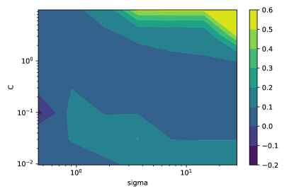
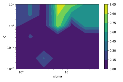
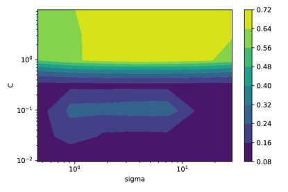
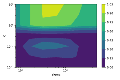
Model and data preparation We used an offset-free SVM classifier with a Gaussian RBF kernel $\kappa(x,y)=\exp(-\lVert x-y\rVert^{2}_{2}/(2\sigma^{2}))$ with RBF width parameter $\sigma>0$. The SVM used the so-called standard SVM-C formulation; the conversion between our and the SVM-C formulation which multiplies the total (hinge) loss by $C>0$ is given by $C=\frac{1}{\lambda n}$ where $n$ is the number of training examples and $\lambda>0$ is the penalty in our formulation (svm). The datasets were split into a training and a test set using the train_test_split method of scikit, keeping $80\%$ of the data for training and $20\%$ for testing.

Model parameters Following the procedure suggested in Section 2.3.1 of Chapelle and Zien [2005], we set up a geometric $7\times 7$ grid over the $(C,\sigma)$-parameter space where $C$ ranges between $2^{-8}C_{0}$ and $2^{2}C_{0}$ and $\sigma$ ranges between $2^{-3}\sigma_{0}$ and $2^{3}\sigma_{0}$, where $\sigma_{0}$ is the median of the Euclidean distance between pairs of data points of the training set, and given $\sigma_{0}$, $C_{0}$ is obtained as the reciprocal value of the empirical variance of data in feature space underlying the RBF kernel with width $\sigma_{0}$. The grid size was selected for economy of computation. The grid lower and upper bounds for $\sigma$ were ad-hoc, though they were inspired by the literature, while for the same for $C$, we enlarged the lower range to focus on the region of the parameter space where the stability-based bounds have a better chance to be effective: In particular, the stability-based bounds grow with $C$ in a linear fashion, with a coefficient that was empirically observed to be close to one.

Computations For each of the $(C,\sigma)$ pairs on the said grid, we trained an SVM-model using a Python implementation of the SMO algorithm of Platt [1999], adjusted to SVMs with no offset (Steinwart2008SVMs argue that “the offset term has neither a known theoretical nor an empirical advantage” for the Gaussian RBF kernel). We then calculated various bounds using the obtained model, as well as the corresponding test error rates (recall that the randomized classifiers’ test error is different than the test error of the SVM model that uses no randomization). The bounds compared were the two mentioned hinge-loss based bounds: The bound by Liu-etal2017SpanishPaper and that of Bousquet and Elisseeff [2002]. In addition we calculated the P@O and (our) P@EW bound. When these latter were calculated we optimized the randomization variance parameter $\sigma_{\text{noise}}^{2}$ by minimizing error estimate obtained from the respective bound (the KL divergence was inverted numerically). Further details of this can be found in Appendix D.

Results As explained earlier our primary interest is to explore the various bounds strengths and weaknesses. In particular, we are interested in their tightness, as well as their ability to support model selection. As the qualitative results were insensitive to the split, results for a single “random” (arbitrary) split are shown only.

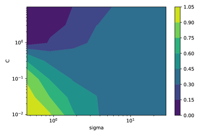
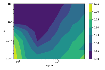
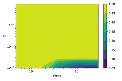
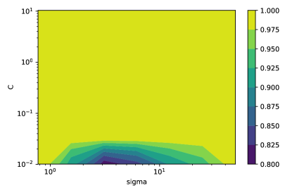
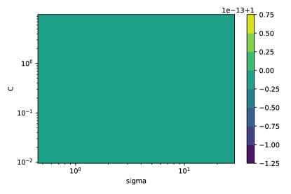
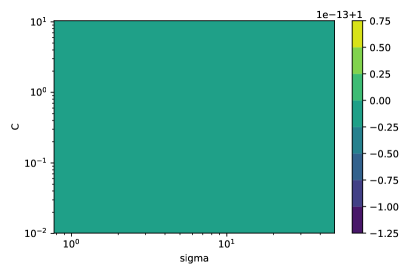
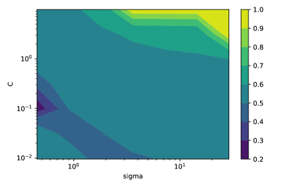
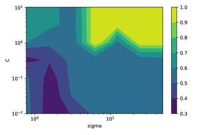
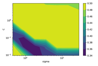
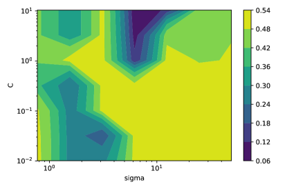
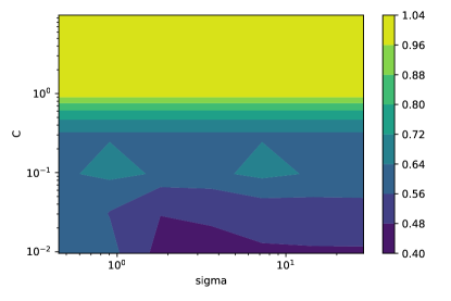
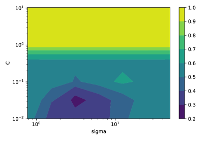
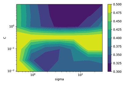
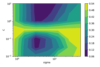
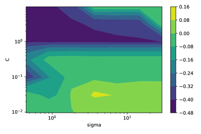
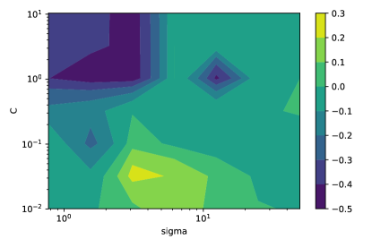
Tightness The hinge loss based bounds gave trivial bounds over almost all pairs of $(C,\sigma)$. Upon investigating this we found that this is because the hinge loss takes much larger values than the training error rate unless $C$ takes large values (cf. Fig. 3 in Appendix D). However, for large values of $C$, both of the bounds are vacuous. In general, the stability based bounds (Liu-etal2017SpanishPaper, Bousquet and Elisseeff [2002] and our bound) are sensitive to large values of $C$. Fig. 1 show the difference between the P@O bound and the test error of the underlying respective randomized classifiers as a function of $(C,\sigma)$ while Fig. 2 shows the difference between the P@EW bound and the test error of the underlying randomized classifier. (Figs. 7 and 9 in the appendix show the test errors for these classifiers, while Figs. 6 and 8 shows the bound.) The meticulous reader may worry about that it appears that on the smaller dataset, pim, the difference shown for P@O is sometimes negative. As it turns out this is due to the randomness of the test error: Once we add a confidence correction that accounts for the randomness of the test small test set ($n_{\text{test}}=154$) this difference disappears once we correct the test error for this. From the figures the most obvious difference between the bounds is that the P@EW bound is sensitive to the value of $C$ and it becomes loose for larger values of $C$. This is expected: As noted earlier, stability based bounds, which P@EW is an instance of, are sensitive to $C$. The P@O bound shows a weaker dependence on $C$ if any. In the appendix we show the advantage (or disadvantage) of the P@EW bound over the P@O bound on Fig. 10. From this figure we can see that on pim, P@EW is to be preferred almost uniformly for small values of $C$ ($C\leq 0.5$), while on rin, the advantage of P@EW is limited both for smaller values of $C$ and a certain range of the RBF width. Two comments are in order in connection to this: (i) We find it remarkable that a stability-based bound can be competitive with the P@O bound, which is known as one of the best bounds available. (ii) While comparing bounds is interesting for learning about their qualities, the bounds can be used together (e.g., at the price of an extra union bound).

Model selection To evaluate a bounds capability in helping model selection it is worth comparing the correlation between the bound and test error of the underlying classifiers. By comparing Figs. 6 and 7 with Figs. 8 and 9 it appears that perhaps the behavior of the P@EW bound (at least for small values of $C$) follows more closely the behavior of the corresponding test error surface. This is particularly visible on rin, where the P@EW bound seems to be able to pick better values both for $C$ and $\sigma$, which lead to a much smaller test error (around $0.12$) than what one can obtain by using the P@O bound.

6 Discussion

We have developed a PAC-Bayes bound for randomized classifiers. We proceeded by investigating the stability of the hypothesis learned by a Hilbert space valued algorithm. A special case being SVMs. We applied our main theorem to SVMs, leading to our P@EW bound, and we compared it to other stability-based bounds and to a previously known PAC-Bayes bound. The main finding is that perhaps P@EW is the first nontrivial bound that uses stability.

Appendix A Proof of Lemma 6

Let $M_{n}=f(Z_{1},\ldots,Z_{n})$ be a function of the independent $\mathcal{Z}$-valued random variables $Z_{1},\ldots,Z_{n}$, where the function $f:\mathcal{Z}^{n}\to\mathcal{H}$ maps into a separable Hilbert space $\mathcal{H}$. Let’s write $M_{n}-\mathbb{E}[M_{n}]$ as the telescopic sum

$$M_{n}-\mathbb{E}[M_{n}]=D_{n}+D_{n-1}+\cdots+D_{1}$$

where

$$D_{i}=\mathbb{E}[M_{n}|\mathcal{F}_{i}]-\mathbb{E}[M_{n}|\mathcal{F}_{i-1}]$$

and $\mathcal{F}_{k}=\sigma(Z_{1},\ldots,Z_{k})$ the $\sigma$-algebra generated by the first $k$ examples. Thus

$$\left\|M_{n}-\mathbb{E}[M_{n}]\right\|^{2}=\sum_{i=1}^{n}\lVert D_{i}\rVert^{2}+2\sum_{i<j}\langle{D_{i}},{D_{j}}\rangle\,.$$

We need $\mathbb{E}\lVert M_{n}-\mathbb{E}[M_{n}]\rVert^{2}$. Taking the expectation above makes the second sum disappear since for $i<j$ we have

$$\mathbb{E}[\langle{D_{i}},{D_{j}}\rangle]=\mathbb{E}\bigl{[}\mathbb{E}[\langle{D_{i}},{D_{j}}\rangle|\mathcal{F}_{i}]\bigr{]}=\mathbb{E}\bigl{[}\langle{D_{i}},{\mathbb{E}[D_{j}|\mathcal{F}_{i}]}\rangle\bigr{]}$$

and clearly $\mathbb{E}[D_{j}|\mathcal{F}_{i}]=0$ for $j>i$. Thus we have

$$\operatorname{\mathbb{E}}\left\|M_{n}-\mathbb{E}[M_{n}]\right\|^{2}=\operatorname{\mathbb{E}}\sum_{i=1}^{n}\lVert D_{i}\rVert^{2}\,.$$ (1)

Also recall the notation $\xi_{k:l}=(\xi_{k},\ldots,\xi_{l})$ for $k<l$. It will be used extensively in what follows.

Let’s write the conditional expectations in terms of regular conditional probabilities:

$$\mathbb{E}[f(Z_{1:n})|\mathcal{F}_{i}]=\int f(Z_{1:i},z_{i+1:n})\hskip 2.0ptdP_{Z_{i+1:n}|Z_{1:i}}(z_{i+1:n}|Z_{1:i})\,.$$

The random variables are labelled with capitals. The lower case letters are for the variables of integration. We write $P_{X}$ for the distribution (probability law) of $X$.

Similarly

$$\mathbb{E}[f(Z_{1:n})|\mathcal{F}_{i-1}] =\int f(Z_{1:i-1},z_{i:n})\hskip 2.0ptdP_{Z_{i:n}|Z_{1:i-1}}(z_{i:n}|Z_{1:i-1})$$

$$=\int f(Z_{1:i-1},z_{i:n})\hskip 2.0ptdP_{Z_{i}|Z_{1:i-1}}(z_{i}|Z_{1:i-1})\cdot\hskip 2.0ptdP_{Z_{i+1:n}|Z_{1:i}}(z_{i+1:n}|Z_{1:i-1},x_{i})\,.$$

By independence, $P_{Z_{i+1:n}|Z_{1:i}}=P_{Z_{i+1:n}}$ and $P_{Z_{i}|Z_{1:i-1}}=P_{Z_{i}}$ (this latter is not really needed in the proof, but shortens the formulae). Hence,

$$D_{i}=\mathbb{E}[f(Z_{1:n})|\mathcal{F}_{i}]-\mathbb{E}[f(Z_{1:n})|\mathcal{F}_{i-1}] =\int f(Z_{1:i},z_{i+1:n})\hskip 2.0ptdP_{Z_{i+1:n}}(z_{i+1:n})$$

$$\hskip 28.45274pt-\int f(Z_{1:i-1},z_{i:n})\hskip 2.0ptdP_{Z_{i}}(z_{i})\hskip 2.0ptdP_{Z_{i+1:n}}(z_{i+1:n})\,.$$

Then $D_{i}$ is equal to the integral w.r.t. $P_{Z_{i+1:n}}(z_{i+1:n})$ of

$$\int[f(Z_{1:i-1},Z_{i},z_{i+1:n})-f(Z_{1:i-1},z_{i},z_{i+1:n})]\hskip 2.0ptdP_{Z_{i}}(z_{i})\,.$$

Notice that in the integrand, only the $i$th argument differs. If $\lVert f(Z_{1:i-1},Z_{i},z_{i+1:n})-f(Z_{1:i-1},z_{i},z_{i+1:n})\rVert\leq c$, then $\lVert D_{i}\rVert\leq c$. Thus bounded differences for $f(Z_{1:n})$ implies bounded martingale differences (in norm).

Finally, using Jensen’s inequality and (1), and the bounded differences assumption:

$$\mathbb{E}\lVert M_{n}-\mathbb{E}[M_{n}]\rVert\leq\sqrt{\mathbb{E}\lVert M_{n}-\mathbb{E}[M_{n}]\rVert^{2}}\leq\sqrt{\sum_{i=1}^{n}c_{i}^{2}}\,.$$

Appendix B The average empirical error for Gaussian random linear classifiers

Let $Q=\mathcal{N}(w_{0},I)$, a Gaussian with center $w_{0}\in\mathbb{R}^{d}$ and covariance matrix the identity $d\times d$. The average empirical error is to be calculated as

$$R(Q,P_{n})=\int_{\mathcal{X}\times\mathcal{Y}}\tilde{F}\left(\frac{y\ w_{0}^{\top}\phi(x)}{\|\phi(x)\|}\right)\hskip 2.0ptdP_{n}(x,y)$$ (2)

where $\tilde{F}=1-F$ and $F$ is the standard normal cumulative distribution

$$F(x)=\int_{-\infty}^{x}{\frac{1}{\sqrt{2\pi}}e^{-u^{2}/2}\hskip 2.0ptdu}\,.$$ (3)

Recall that $P_{n}=\frac{1}{n}\sum_{i=1}^{n}\delta_{(X_{i},Y_{i})}$ is the empirical measure on $\mathcal{X}\times\mathcal{Y}$ associated to the $n$ training examples, and the integral with respect to $P_{n}$ evaluates as a normalized sum.

In this section we write the derivation of (2).

To make things more general let $Q=\mathcal{N}(w_{0},\Sigma)$, a Gaussian with center $w_{0}\in\mathbb{R}^{d}$ and covariance matrix $\Sigma$. We’ll write $G_{(w_{0},\Sigma)}$ for the corresponding Gaussian measure on $\mathbb{R}^{d}$. But to make notation simpler, lets work with input vectors $x$ (instead of feature vectors $\phi(x)\in\mathcal{H}$). This is in the context of binary classification, so the labels are $y\in\{\pm 1\}$. The classifier $c_{w}(\cdot)=\operatorname{sign}(\langle w,\cdot\rangle)$ is identified with the weight vector $w$. The loss on example $(x,y)$ can be written as

$$\ell(c_{w}(x),y)=\mathbf{1}(c_{w}(x)\neq y)=\frac{1-\operatorname{sign}(y\langle w,x\rangle)}{2}\,.$$

We’ll talk about the empirical error of $w$, namely $R(w,P_{n})=\int_{\mathcal{X}\times\mathcal{Y}}\mathbf{1}(c(x)\neq y)\hskip 2.0ptdP_{n}(x,y)$. The average empirical error when choosing a random weight $W$ according to $Q$ is:

$$R(Q,P_{n})=\int_{\mathbb{R}^{d}}R(w,P_{n})\hskip 2.0ptdG_{(w_{0},\Sigma)}(w)\,.$$

Plugging in the definition of $R(w,P_{n})$ and swapping the order of the integrals and using the above formula for the loss, the right hand side is

$$\int_{\mathbb{R}^{d}}\int_{\mathcal{X}\times\mathcal{Y}}\mathbf{1}(c(x)\neq y)\hskip 2.0ptdP_{n}(x,y) \hskip 2.0ptdG_{(w_{0},\Sigma)}(w)$$

$$=\int_{\mathcal{X}\times\mathcal{Y}}\int_{\mathbb{R}^{d}}\mathbf{1}(c(x)\neq y)\hskip 2.0ptdG_{(w_{0},\Sigma)}(w)\hskip 2.0ptdP_{n}(x,y)$$

$$=\int_{\mathcal{X}\times\mathcal{Y}}\int_{\mathbb{R}^{d}}\frac{1-\operatorname{sign}(y\langle w,x\rangle)}{2}\hskip 2.0ptdG_{(w_{0},\Sigma)}(w)\hskip 2.0ptdP_{n}(x,y)$$

$$=\int_{\mathcal{X}\times\mathcal{Y}}\frac{1}{2}\left(1-A(x,y)\right)\hskip 2.0ptdP_{n}(x,y)$$

where for a fixed pair $(x,y)$ we are writing

$$A(x,y)=\int_{\mathbb{R}^{d}}\operatorname{sign}(y\langle w,x\rangle)\hskip 2.0ptdG_{(w_{0},\Sigma)}(w)\,.$$

Decompose into two terms:

$$A(x,y)=\int_{y\langle w,x\rangle>0}\!\!\!\hskip 2.0ptdG_{(w_{0},\Sigma)}(w)-\int_{y\langle w,x\rangle<0}\!\!\!\hskip 2.0ptdG_{(w_{0},\Sigma)}(w)$$

and notice that for the random vector $W\sim\mathcal{N}(w_{0},\Sigma)$ we have $\mathbb{E}[y\langle W,x\rangle]=y\langle w_{0},x\rangle$ and $\mathbb{E}[(y\langle W,x\rangle)^{2}]=\|x\|_{\Sigma}^{2}+(\langle w_{0},x\rangle)^{2}$, so the functional $y\langle W,x\rangle$ has a 1-dimensional Gaussian distribution with mean $y\langle w_{0},x\rangle$ and variance $\|x\|_{\Sigma}^{2}=\langle\Sigma x,x\rangle$. Then

$$\int_{y\langle w,x\rangle>0}\hskip 2.0ptdG_{(w_{0},\Sigma)}(w) =\operatorname{Pr}[y\langle W,x\rangle>0]$$

$$=\operatorname{Pr}\left[\frac{y\langle W,x\rangle-y\langle w_{0},x\rangle}{\|x\|_{\Sigma}}>\frac{-y\langle w_{0},x\rangle}{\|x\|_{\Sigma}}\right]$$

$$=\operatorname{Pr}\left[\mathcal{N}(0,1)>\frac{-y\langle w_{0},x\rangle}{\|x\|_{\Sigma}}\right]$$

$$=\operatorname{Pr}\left[\mathcal{N}(0,1)<\frac{y\langle w_{0},x\rangle}{\|x\|_{\Sigma}}\right]=F\left(\frac{y\langle w_{0},x\rangle}{\|x\|_{\Sigma}}\right)\,.$$

Then

$$A(x,y)=2F\left(\frac{y\langle w_{0},x\rangle}{\|x\|_{\Sigma}}\right)-1$$

and

$$1-A(x,y)=2-2F\left(\frac{y\langle w_{0},x\rangle}{\|x\|_{\Sigma}}\right)=2\tilde{F}\left(\frac{y\langle w_{0},x\rangle}{\|x\|_{\Sigma}}\right)\,.$$

Altogether this gives

$$R(Q,P_{n})=\int_{\mathcal{X}\times\mathcal{Y}}\tilde{F}\left(\frac{y\langle w_{0},x\rangle}{\|x\|_{\Sigma}}\right)\hskip 2.0ptdP_{n}(x,y)\,.$$

Notice that using $\Sigma=I$ (identity) and $\phi(x)$ instead of $x$ this gives (2).

REMARK: Langford [2005] uses a $Q$ which is $\mathcal{N}(\mu,1)$ along the direction of a vector $w$, and $\mathcal{N}(0,1)$ in all directions perpendicular to $w$. Such $Q$ is a Gaussian centered at $w_{0}=\mu w/\|w\|$, giving his formula

$$R(Q,P_{n})=\int_{\mathcal{X}\times\mathcal{Y}}\tilde{F}\left(\mu\frac{y\ w^{\top}\phi(x)}{\|w\|\ \|\phi(x)\|}\right)\hskip 2.0ptdP_{n}(x,y)\,.$$

Appendix C SVM weight vector: clarification about formulations

We have a sample of size $n$.

In the standard implementation the weight vector $W_{n}(C)$ found by $\operatorname{SVM}$ is a solution of the following optimization problem:

$$W_{n}(C)=\operatorname*{arg\,min}_{w}\biggl{(}\frac{1}{2}\lVert w\rVert_{\mathcal{H}}^{2}+C\sum_{i=1}^{n}\xi_{i}\biggr{)}\,.$$ (svm1)

In our paper the weight vector $W_{n}^{\textrm{OURS}}(\lambda)$ found by $\operatorname{SVM}$ is a solution of the following optimization problem:

$$W_{n}^{\textrm{OURS}}(\lambda)=\operatorname*{arg\,min}_{w}\biggl{(}\frac{\lambda}{2}\lVert w\rVert_{\mathcal{H}}^{2}+\frac{1}{n}\sum_{i=1}^{n}\xi_{i}\biggr{)}\,.$$ (svm2)

In Bousquet and Elisseeff [2002] and Liu et al. [2017] the weight vector $W_{n}^{\textrm{B\&E}}(\lambda)$ found by $\operatorname{SVM}$ is a solution of the following optimization problem:

$$W_{n}^{\textrm{B\&E}}(\lambda)=\operatorname*{arg\,min}_{w}\biggl{(}\lambda\lVert w\rVert_{\mathcal{H}}^{2}+\frac{1}{n}\sum_{i=1}^{n}\xi_{i}\biggr{)}\,.$$ (svm3)

The minimum is over $w\in\mathcal{H}$ (an appropriate Hilbert space) and subject to some constrains for the $\xi_{i}$’s in all cases.

The relation between them is:

• $W_{n}^{\textrm{OURS}}(\lambda)=W_{n}^{\textrm{B\&E}}(\lambda/2)$

• $W_{n}^{\textrm{B\&E}}(\lambda)=W_{n}(C)$ with $C=\frac{1}{2n\lambda}$

• $W_{n}^{\textrm{OURS}}(\lambda)=W_{n}(C)$ with $C=\frac{1}{n\lambda}$

Appendix D Details for experiments

In this section we show further details and results that did not fit the main body of the paper.

D.1 Details of optimizing $\sigma_{\text{noise}}^{2}$

This optimization is “free” for the P@O bound as the bound is uniform over $\sigma_{\text{noise}}^{2}$. In the P@EW bound we adjusted the failure probability $\delta$ to accommodate the multiple evaluations during the optimization by replacing it with $\delta/(\tau(\tau+1))$, where $\tau$ is the number of times the P@EW bound is evaluated by the optimization procedure. A standard union bound argument shows that the adjustment to $\delta$ makes the resulting bound hold with probability $1-\delta$ regardless the value of $\tau$. The SLSQP method implemented in scipy was used as an optimizer, with an extra outer loop that searched for a suitable initialization, as SLSQP is a gradient based method and the P@O bound can be quite “flat”. The same problem did not appear for the P@EW bound. The attentive reader may be concerned that if $\tau$ gets large values, we, in a way, are optimizing the “wrong bound”. To check whether this is a possibility, we also computed the “union bound penalty” for decreasing $\delta$ by the factor $\tau(\tau+1)$ as the difference between the (invalid) bound where $\delta$ is unchanged and the bound where $\delta$ is decreased and found that the penalty was generally orders of magnitudes smaller than the risk estimate. Nevertheless, this may be a problem when the risk to be estimated is very small, which we think is not very common in practice.

D.2 Additional figures

Figure 3: Hinge loss on pim (left) and rin (right). For large values of $C$, the hinge loss is reasonable, but this is not the case for small values.

Figure 4: The bound of Liu-etal2017SpanishPaper on pim (left) and rin (right). The bound is almost always vacuous for reasons described in the text.

Figure 5: The bound of Bousquet and Elisseeff [2002] on pim (left) and rin (right). The bound is almost always vacuous for reasons described in the text.

Figure 6: The P@O bound on pim (left) and rin (right).

Figure 7: Test error of the randomized classifiers underlying the P@O bound on pim (left) and rin (right).

Figure 8: The P@EW bound on pim (left) and rin (right).

Figure 9: Test error of the randomized classifiers underlying the P@EW bound on pim (left) and rin (right).

Figure 10: Advantage of the P@EW bound to the P@O bound on pim (left) and rin (right): The figure shows the difference between the P@O bound and the P@EW bound. Where this is positive, P@EW is to be preferred, while where it is negative, P@O is to be preferred.

Appendix E Gaussian distributions over the Hilbert space of classifiers?

The idea behind PAC-Bayes is that instead of the weight vector $W_{n}=\operatorname{SVM}(S_{n})$ we randomize by choosing a fresh $W\in\mathcal{H}$ according to some probability distribution on $\mathcal{H}$ for each prediction.

With the Gaussian kernel in mind, we are facing an infinite-dimensional separable $\mathcal{H}$, which upon the choice of an orthonormal basis $\{e_{1},e_{2},\ldots\}$ can be identified with the space $\ell_{2}\subset\mathbb{R}^{\mathbb{N}}$ of square summable sequences of real numbers, via the isometric isomorphism $\mathcal{H}\to\ell_{2}$ that maps the vector $w=\sum_{i=1}^{\infty}w_{i}e_{i}\in\mathcal{H}$ to the sequence $(w_{1},w_{2},\ldots)\in\ell_{2}$. Thus without loss of generality we will regard the feature map as $\phi:\mathcal{X}\to\ell_{2}\subset\mathbb{R}^{\mathbb{N}}$.

Suppose the randomized classifier $W$ is to be chosen according to a Gaussian distribution.

Two possibilities come to mind for the choice of random classifier $W$: (1) according to a Gaussian measure on $\ell_{2}$, say $W\sim\mathcal{N}(\mu,\Sigma)$ with mean $\mu\in\ell_{2}$ and covariance operator $\Sigma$ meeting the requirements (positive, trace-class) for this to be a Gaussian measure on $\ell_{2}$; or (2) according to a Gaussian measure on the bigger $\mathbb{R}^{\mathbb{N}}$, e.g. $W\sim\mathcal{N}(\mu,I)$ by which we mean the measure constructed as the product of a sequence $\mathcal{N}(\mu_{i},1)$ of independent real-valued Gaussians with unit variance. These two possibilities are mutually exclusive since the first choice gives a measure on $\mathbb{R}^{\mathbb{N}}$ whose mass is supported on $\ell_{2}$, while the second choice leads to a measure on $\mathbb{R}^{\mathbb{N}}$ supported outside of $\ell_{2}$. A good reference for these things is Bogachev [1998].

Let’s go with the second choice: $\mathcal{N}(0,I)=\bigotimes_{i=}^{\infty}\mathcal{N}(0,1)$, a ‘standard Gaussian’ on $\mathbb{R}^{\mathbb{N}}$. This is a legitimate probability measure on $\mathbb{R}^{\mathbb{N}}$ (by Kolmogorov’s Extension theorem). But it is supported outside of $\ell_{2}$, so when sampling a $W\in\mathbb{R}^{\mathbb{N}}$ according to this measure, with probability one such $W$ will be outside of our feature space $\ell_{2}$. Then we have to wonder about the meaning of $\langle W,\cdot\rangle$ when $W$ is not in the Hilbert space carrying this inner product.

Let’s write $W=(\xi_{1},\xi_{2},\ldots)$ a sequence of i.i.d. standard (real-valued) Gaussian random variables. Let $x=(x_{1},x_{2},\ldots)\in\ell_{2}$, and consider the formal expression $\langle x,W\rangle=\sum_{i=1}^{\infty}x_{i}\xi_{i}$. Notice that

$$\sum_{i=1}^{\infty}\mathbb{E}[|x_{i}\xi_{i}|^{2}]=\sum_{i=1}^{\infty}|x_{i}|^{2}<\infty\,.$$

Then (see e.g. Bogachev [1998], Theorem 1.1.4) our formal object $\langle x,W\rangle=\sum_{i=1}^{\infty}x_{i}\xi_{i}$ is actually well-defined in the sense that the series is convergent almost surely (i.e. with probability one), although as we pointed out such $W$ is outside $\ell_{2}$.

E.1 Predicting with the Gaussian random classifier

Let $W_{n}=\operatorname{SVM}(S_{n})$ be the weight vector found by running SVM on the sample $S_{n}$. We write it as $W_{n}=\sum_{i=1}^{n}\alpha_{i}Y_{i}\phi(X_{i})$.

Also as above let $W$ be a Gaussian random vector in $\mathbb{R}^{\mathbb{N}}$, and write it as $W=\sum_{j=1}^{\infty}\xi_{j}e_{j}$ with $\xi_{1},\xi_{2},\ldots$ i.i.d. standard Gaussians. As usual $e_{j}$ stands for the canonical unit vectors having a 1 in the $j$th coordinate and zeros elsewhere.

For an input $x\in\mathcal{X}$ with corresponding feature vector $\phi(x)\in\mathcal{H}$, we predict with

$$\langle W_{n}+W,\phi(x)\rangle=\sum_{i=1}^{n}\alpha_{i}Y_{i}\kappa(X_{i},x)+\sum_{j=1}^{\infty}\xi_{j}\langle e_{j},\phi(x)\rangle\,.$$

This is well-defined since

$$\sum_{i=1}^{\infty}\mathbb{E}[(\xi_{j}\langle e_{j},\phi(x)\rangle)^{2}]=\sum_{i=1}^{\infty}(\langle e_{j},\phi(x)\rangle)^{2}=\|\phi(x)\|^{2}\,,$$

so the series $\sum_{j=1}^{\infty}\xi_{j}\langle e_{j},\phi(x)\rangle$ converges almost surely (Bogachev [1998], Theorem 1.1.4).

References

- Abou-Moustafa and Szepesvari [2017] Karim Abou-Moustafa and Csaba Szepesvari. An a priori exponential tail bound for k-folds cross-validation. ArXiv e-prints, 2017.
- Bogachev [1998] Vladimir I. Bogachev. Gaussian Measures. American Mathematical Society, 1998.
- Bousquet and Elisseeff [2002] Olivier Bousquet and André Elisseeff. Stability and generalisation. Journal of Machine Learning Research, 2:499–526, 2002.
- Catoni [2007] Olivier Catoni. PAC-Bayesian supervised classification: the thermodynamics of statistical learning. Technical report, Institute of Mathematical Statistics, Beachwood, Ohio, USA, 2007.
- Celisse and Guedj [2016] Alain Celisse and Benjamin Guedj. Stability revisited: new generalisation bounds for the leave-one-out. arXiv preprint arXiv:1608.06412, 2016.
- Chapelle and Zien [2005] Olivier Chapelle and Alexander Zien. Semi-supervised classification by low density separation. In AISTATS, 2005.
- Dziugaite and Roy [2017] Gintare Karolina Dziugaite and Daniel M Roy. Computing nonvacuous generalization bounds for deep (stochastic) neural networks with many more parameters than training data. arXiv preprint arXiv:1703.11008, 2017.
- Freund [1998] Yoav Freund. Self bounding learning algorithms. In Proceedings of the eleventh annual conference on Computational learning theory, pages 247–258. ACM, 1998.
- Germain et al. [2009] Pascal Germain, Alexandre Lacasse, François Laviolette, and Mario Marchand. PAC-Bayesian learning of linear classifiers. In Proc. of the 26th International Conference on Machine Learning, pages 353–360. ACM, 2009.
- Germain et al. [2015] Pascal Germain, Alexandre Lacasse, Francois Laviolette, Mario Marchand, and Jean-Francis Roy. Risk bounds for the majority vote: From a PAC-Bayesian analysis to a learning algorithm. Journal of Machine Learning Research, 16:787–860, 2015.
- Kontorovich [2014] Aryeh Kontorovich. Concentration in unbounded metric spaces and algorithmic stability. In Proc. of the 31st International Conference on Machine Learning, pages 28–36, 2014.
- Langford [2005] John Langford. Tutorial on practical prediction theory for classification. Journal of Machine Learning Research, 6(Mar):273–306, 2005.
- Langford and Blum [2003] John Langford and Avrim Blum. Microchoice bounds and self bounding learning algorithms. Machine Learning, 51(2):165–179, 2003.
- Lever et al. [2010] Guy Lever, François Laviolette, and John Shawe-Taylor. Distribution-dependent PAC-Bayes priors. In International Conference on Algorithmic Learning Theory, pages 119–133. Springer, 2010.
- Liu et al. [2017] Tongliang Liu, Gábor Lugosi, Gergely Neu, and Dacheng Tao. Algorithmic stability and hypothesis complexity. In Proc. of the 34th International Conference on Machine Learning, pages 2159–2167, 2017.
- London [2017] Ben London. A PAC-Bayesian analysis of randomized learning with application to stochastic gradient descent. In Advances in Neural Information Processing Systems, pages 2931–2940, 2017.
- London et al. [2013] Ben London, Bert Huang, Ben Taskar, and Lise Getoor. Collective stability in structured prediction: Generalization from one example. In Proc. of the 30th International Conference on Machine Learning, pages 828–836, 2013.
- Lugosi and Pawlak [1994] Gábor Lugosi and Miroslaw Pawlak. On the posterior-probability estimate of the error rate of nonparametric classification rules. IEEE Transactions on Information Theory, 40(2):475–481, 1994.
- Parrado-Hernández et al. [2012] Emilio Parrado-Hernández, Amiran Ambroladze, John Shawe-Taylor, and Shiliang Sun. PAC-Bayes bounds with data dependent priors. Journal of Machine Learning Research, 13:3507–3531, 2012.
- Platt [1999] John C. Platt. Fast training of support vector machines using sequential minimal optimization. In B. Schölkopf, C. J. C. Burges, and A. J. Smola, editors, Advances in Kernel Methods – Support Vector Learning, pages 185–208. MIT Press, Cambridge MA, 1999.
- Shawe-Taylor and Cristianini [2004] John Shawe-Taylor and Nello Cristianini. Kernel Methods for Pattern Analysis. Cambridge University Press, Cambridge, UK, 2004.
- Steinwart and Christmann [2008] Ingo Steinwart and Andreas Christmann. Support Vector Machines. Springer Science & Business Media, 2008.