22email: moyerd@usc.edu
Measures of Tractography Convergence
Abstract
In the present work, we use information theory to understand the empirical convergence rate of tractography, a widely-used approach to reconstruct anatomical fiber pathways in the living brain. Based on diffusion MRI data, tractography is the starting point for many methods to study brain connectivity. Of the available methods to perform tractography, most reconstruct a finite set of streamlines, or 3D curves, representing probable connections between anatomical regions, yet relatively little is known about how the sampling of this set of streamlines affects downstream results, and how exhaustive the sampling should be. Here we provide a method to measure the information theoretic surprise (self-cross entropy) for tract sampling schema. We then empirically assess four streamline methods. We demonstrate that the relative information gain is very low after a moderate number of streamlines have been generated for each tested method. The results give rise to several guidelines for optimal sampling in brain connectivity analyses.
Keywords:
Tractography, Cross Entropy, Simulation1 Introduction
It is common practice in brain imaging studies to estimate the trajectories of white matter fascicles, the bundles of axons that connect different gray matter regions in the brain. It is difficult to observe the fascicles directly in vivo; instead, researchers currently rely on diffusion imaging - a variant of standard anatomical MRI - and the “tube like” structure of most major neural pathways to reconstruct the brain’s major fiber bundles. We observe measurements of water diffusion in brain tissue, fit local diffusion models, and then reconstruct the trajectories by curve fitting. This process is known as tractography, and reconstructed fibers are referred to as tracts111It is important to distinguish between white matter fibers (fascicles) and observed “tracts.” In this paper we use “tracts” to denote the 3D-curves recovered from diffusion-weighted imaging via tractography algorithms..
The number of possible curves is combinatorially large, and grows rapidly as image resolution increases. Closed form likelihoods for sets of tracts (tractograms) have not yet been found even under simple local models. Thus, tract sampling is performed, where only a subset of the possible tracts are recovered. Sampling is usually performed in an ad-hoc manner, and post-hoc analyses usually treat tracts as direct observations instead of realizations of global trajectories from local models. The concept that tracts are drawn from a distribution is rarely acknowledged, and the issue of convergence is almost never addressed.
A simple question remains unanswered: how many tracts should we sample? Even in the most general sense there is no consensus on this topic. Recent works have used 100,000 [11], 500,000 [10] and 10,000,000 [18] tracts for scans of isotropic resolution 2 mm (with 64 directions), 1.25 mm (90 directions), and 2.5 mm (60 directions), respectively. The pragmatic tractography user might then think to simply take the maximum of these options to ensure convergence; for small studies this may be feasible, but given the trajectory of imaging studies - now performed in biobanks of over 10,000 scans - this choice clearly will not scale to the regimes demanded by current and future clinical studies222The largest study to date aims to have 100,000 subjects participating in the imaging cohort [15]. By our back-of-the-envelope estimate, 100,000 subjects with 10,000,000 tracts each would require about 1.5 petabytes of disk space, just for the tractograms. using current technology. The answer to whether or not such large tractogram sizes are required will dictate practical planning in large studies.
It is useful then to understand empirically the sample complexity of these phenomena. If we choose a sample size too small our tractograms will be sensitive random fluctuations; if instead we choose a sample size too large, we could be wasting very large amounts of storage and computation. The trade-off between accuracy and cost forms a curve of solutions to the (ill-posed) question of “how many tracts?” In the present work we provide a method for measuring this trade-off. We leverage cross entropy as a relative measure of accuracy, applying our estimator to a test set of subjects under several different tractography methods.
1.1 Relevant Prior Work
Surprisingly literature on the number of samples required is sparse. In the documentation of Probtrackx [2] the number of posterior samples is taken to be large (5,000 per vertex) specifically to ensure convergence. This solution is not feasible for most other methods, as Probtrackx does not usually keep computed trajectories, but is the most direct reference to tractogram convergence that we found in the literature.
In Cheng et al. [3] the authors address the convergence of network measures. While this is a similar issue, it is seen through the lens of graph theory. In a network context the absolute (objective) number of tracts strongly influences the downstream measures. Thus, the authors advise against larger numbers of seeds in order to avoid spurious fibers. Similarly, Prasad et al. [17] investigate effect of the number of streamlines used on a group-wise comparison task. The authors note that larger numbers of streamlines tend to decrease p-values in nodal degree comparisons.
Similar to this, Maier et al. [14] provide a tractography challenge in which the measure of success depends in part on how few false positives were identified. This work is an important if not critical step for the community to address issues raised by others (e.g., Thomas et al. [20]), but its evaluation design runs counter to our premise here that tractography is a simulation. It is equivalent to taking the support of the distribution as its characterizing quality.
Jordan et al. [12] propose a method for measuring streamline reproducibility. This method is essentially the same as proposed here, using a KDE-like form to assign a weight (density) to each streamline. The authors do not identify this as a KDE (and accordingly use a non-standard power-law kernel), but otherwise produce the same method.
2 Framework and Methods
2.1 Minimal Surprise as a stopping condition
Diffusion MRI does not provide direct observations of whole white matter fascicles; the unit of observation is a -space measurement of diffusion propensity for given gradient angles, which is resolved and processed into quantized voxel measurements. Researchers simulate fascicle trajectories from fitted local (voxel-wise) models, which have parameters estimated from the diffusion signal (for reference and review, see Sotiropoulos and Zalesky [19]). Some of these simulations are deterministic given a seed point, while others are stochastic. In both cases, however, seed points are not bijective with tracts. If the choice of seed point is random, it is then reasonable to view the tractography generation process as sampling from a distribution defined over the space of possible tracts, stratified by seed points.
The space of possible tracts has at minimum a qualitative notion of similarity. While there is no agreed upon metric, various distances and similarities have been proposed [16, 23, 8]. Choosing a reasonable metric, a simplistic estimator of tract distributions can be constructed using Kernel Density Estimation (KDE). These estimators enjoy concentration results333In short, we are asserting that converges as the number of samples used to construct it increases. This does not guarantee that converges to . even in our general context [4] with minimal constraints on metric choice or kernel shape. The construction of distribution estimates lead us to a naïve condition for assessing convergence: we should stop sampling when stops gaining information (“stops learning”).
is a representation of our beliefs about . A sample from containing information not in (i.e., contrary to our beliefs) is then qualitatively surprising. As we update our beliefs we learn about ; when the surprise no longer decreases we have stopped updating our beliefs, so we have stopped gaining information, which is exactly our stopping condition. Thus we should sample until we have minimal surprise.
Before moving on, it should be made explicit: clearly will be misspecified. Without a natural metric, it is not clear if an estimator class could ever be guaranteed to include in every case. With this in mind, our provided method is left open-ended toward choice of metric, kernel shape, smoothing parameter, etc. Further, for different datasets, the convergence rate of will be different. Higher resolution data will provide more information, providing more intrinsic information in , meaning has more surprise to overcome. The point of this paper is not to estimate exactly, nor to establish objective numerical standards for the number of tracts for every case, but to provide a method to investigate the complexity of tract generation. It is our belief that with reasonable choices a conservative estimate can be made to the number of samples required.
2.2 Quantitative Measures of Surprise
Kullback-Leibler divergence (KL divergence) is a classic measurement for the differences between distributions. While it has numerous interpretations and applications, in the information theory context it measures the “extra information” required to encode samples drawn from using the optimal encoding for [5]. This is often used as a pseudo-distance, as “close” distributions have similar optimal encodings.
KL divergence has the following analytic form, with by convention:
| (1) | ||||
| (2) |
For any the Negative Entropy term is clearly fixed, regardless of . Following our previous intuition, this corresponds to the intrinsic surprise of , the number of bits required to encode under the optimal encoding. The Cross Entropy term corresponds to the induced surprise of using ’s encoding in place of . It is thus our desired measure of surprise; measuring Cross Entropy is the focus of our empirical method. Both have units of bits (or nats) of information.
2.3 Fixed-KDE Cross Entropy
We construct a simple estimator of Cross Entropy using Kernel Density Estimation (KDE). Let be samples from a distribution , and let be a metric. The (unnormalized) squared exponential kernel function for distance is defined as
| (3) |
Using this function, we can then define an unnormalized Gaussian KDE:
| (4) |
We use to emphasize that this distribution is off by a normalizing constant, and to denote that this is an estimate of based on . We assume there exists a finite normalization constant, . An approximation of the distribution of tracts is then
| (5) |
Using Eq. 5, we can form an approximation to the Cross Entropy up to a constant.
| (6) | ||||
| (7) | ||||
| (8) |
2.4 Calculating Tract Sample Cross Entropy
Several metric spaces have been proposed [16, 8] for streamlines. These allow us to apply our KDE estimator to the streamline distributions. We use the MDF distance of Garyfallidis et al. [8] as the distance metric in Eq. 3. We then estimate the Cross-Entropy of samples to tract distributions in these spaces using Eq. 8. While Eq. 8 is always off by an unknown constant, the rate of information gain is preserved. This allows us to measure the marginal value (in bits) of increasing sample sizes. Further, for fixed the objective information content is comparable across distributions.
As tracts are simulated and each observation is independent, many issues are simplified in our approximation. In particular, we separate the and samples, letting the number of be large () no matter the choice of (the number of ) in order to ensure a good estimate of the outer expectation. We can further separate the kernel computation step and the summation step, which allows for fast bootstrap estimates as well as faster computation for increasing sizes of .
2.5 Scale Considerations
Note that each KDE used fixed and un-tuned bandwidth . Thus, our KDE converges to instead of , where . We believe this to be a feature and not a bug: first, though the tractography simulation is often conducted with high numerical precision (using, e.g., floating point representation), the trajectories of streamlines are determined in part by the diffusion measurements. These measurements are ill-resolved relative to machine precision. Second, later analyses of streamline distributions are rarely conducted at a local scale. Fixing allows for “convergence” to be contextualized to a particular spatial scale, albeit after the choice of a tract metric. Thus, if the practitioner does not need to resolve small scale differences, a corresponding choice of can be made.
3 Empirical Assessment
We apply the Cross Entropy estimator to 44 test subjects from the publicly available Human Connectome Project dataset [22]. We used the minimally preprocessed T1-weighted (T1w) and diffusion-weighted (DWI) images rigidly aligned to MNI 152 space. Briefly, the preprocessing of these images included gradient nonlinearity correction (T1w, DWI), motion correction (DWI), eddy current correction (DWI), and linear alignment (T1w, DWI). We used the HCP Pipeline FreeSurfer [6] protocol, running the recon-all pipeline.
Tractography was conducted using the DWI in 1.25-mm isotropic MNI 152 space. Three separate types of tractography were conducted, using three separate local models and two different tracking methods. All three were performed using the Dipy [9] implementation. The local models were as follows:
-
1.
Constrained Spherical Deconvolution (CSD) [21] with a harmonic order of 8
-
2.
Constant Solid Angle (CSA) [1] with a harmonic order of 8
-
3.
Diffusion Tensors (DTI) (see, e.g., [13])
Probabilistic streamline tractography was performed using Dipy’s probabilistic direction getter for CSD and CSA local models, while deterministic tracking was completed using EuDX [7] for DTI and the Local Tracking module for CSD. For each local model streamlines were then seeded at 2 million random locations (total) in voxels labeled as likely white matter by FSL’s FAST [24] and propagated in 0.5 mm steps, constrained to at most angles between segments. Each set of tracts was split into two equally sized subsets. Cross-entropy was then calculated using Eq. 8 for five separate length-scale choices , using 1000 streamline intervals to allow for parallelization and efficient storage. This portion of the procedure was written in C++ with OpenMP444Please contact the authors to access the code..
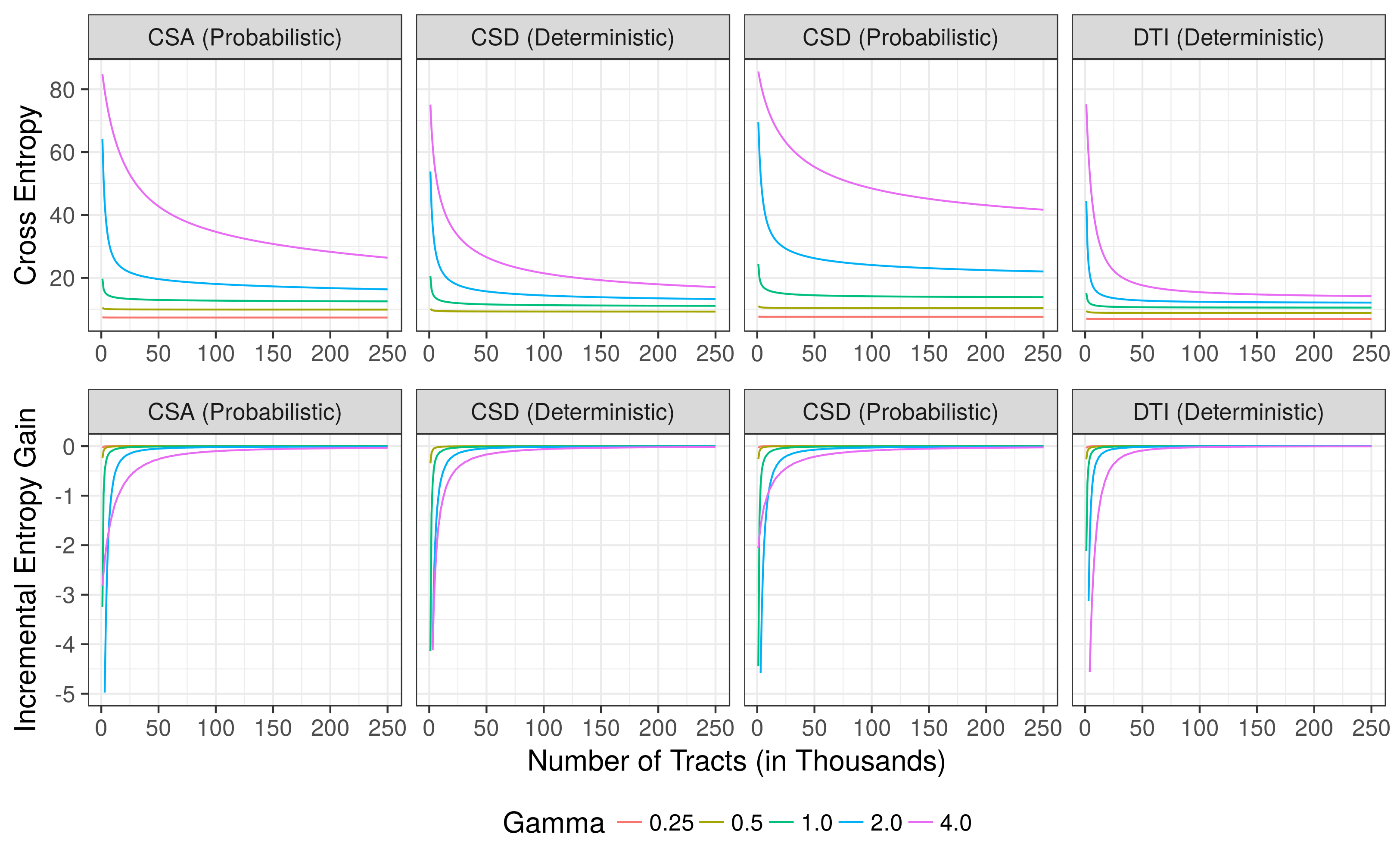

In the top row of Fig. 1 we plot the cross-entropy (surprise) as a function of the number of samples when sampling at random from within the white matter mask. The curve for is nearly flat, while for and the curves quickly bottom out after a short steep learning period. As the length scale increases, the learning rate becomes quite slow. At the curves begin to bottom out at 250000 samples. However, for each of these scales, no significant changes occur after 500000 samples. If there is relevant signal in these samples that is not contained on average in the previous half-million samples, it has a very small relative amount of information about the distribution of tracts.
In general for each length scale both deterministic methods have less entropy than the probabilistic methods. Further, DTI converges (flattens) much faster than the other methods. These results match our prior intuitions about these methods. Probabilistic CSD has the largest information content, though we condition this in that in general noise adds information, albeit useless information. Thus, this is not alone a measure of quality, though it does differentiate the method as certainly sampling a tract distribution unlike the others.
In the bottom row of Fig. 1 we plot the incremental (marginal) entropy rate. For each length scale for each method the marginal information gained per thousand streamlines after the initial learning period is very low; this is unsurprising, but raises questions about the utility of sampling past several million tracts.
These curves are artificially smooth due to the binning of the number of samples by thousands; while in each plot the curves are monotonic, this is an overall trend (at the scale of thousands of samples) and not true locally (at the scale of single samples).
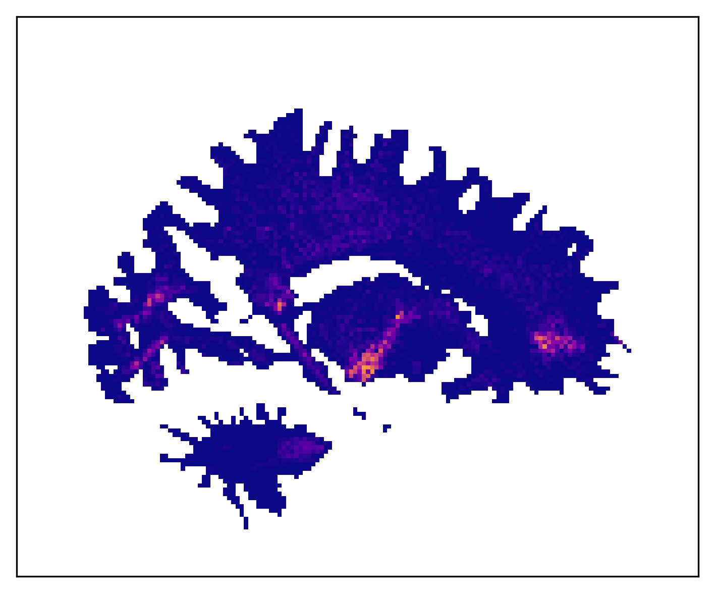
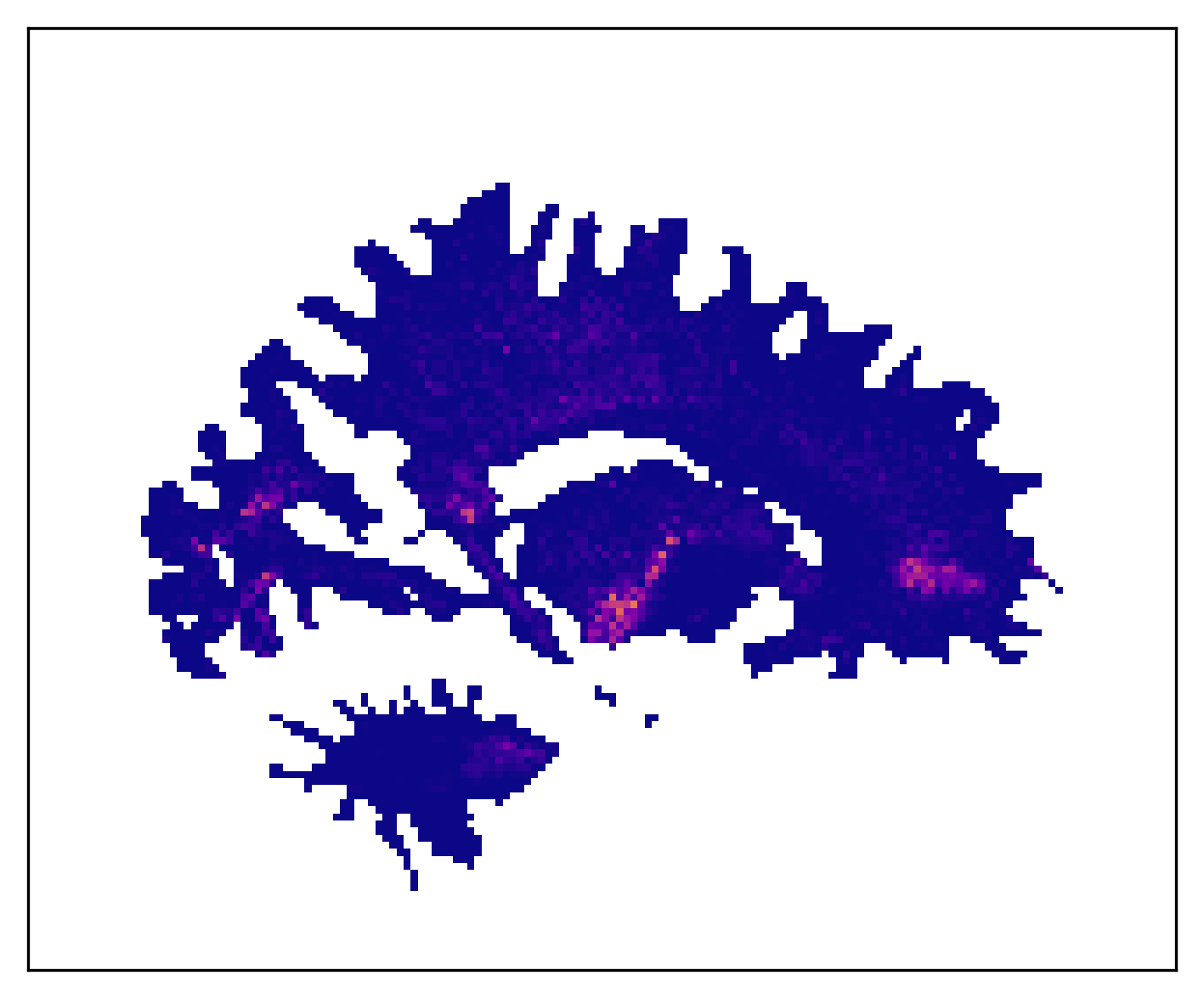
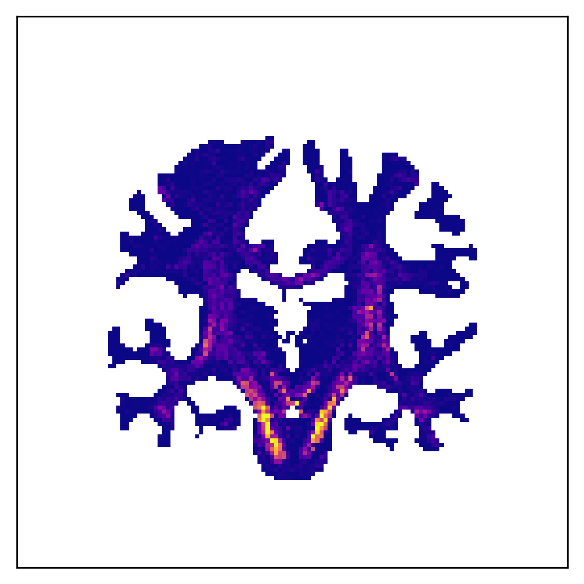
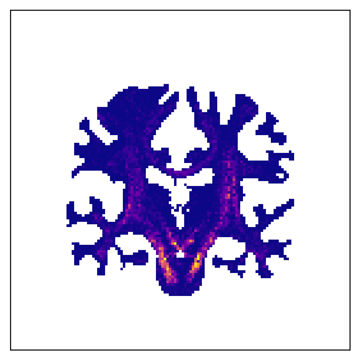
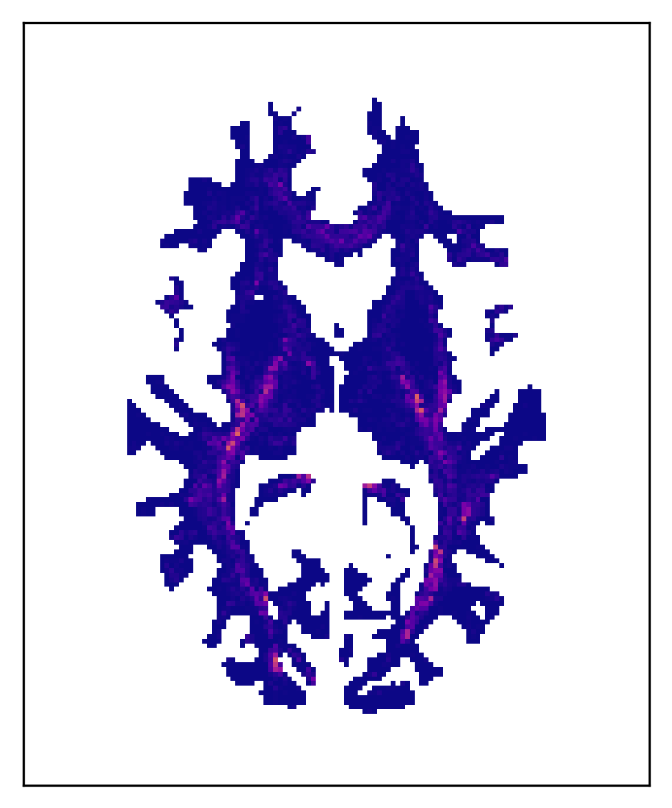
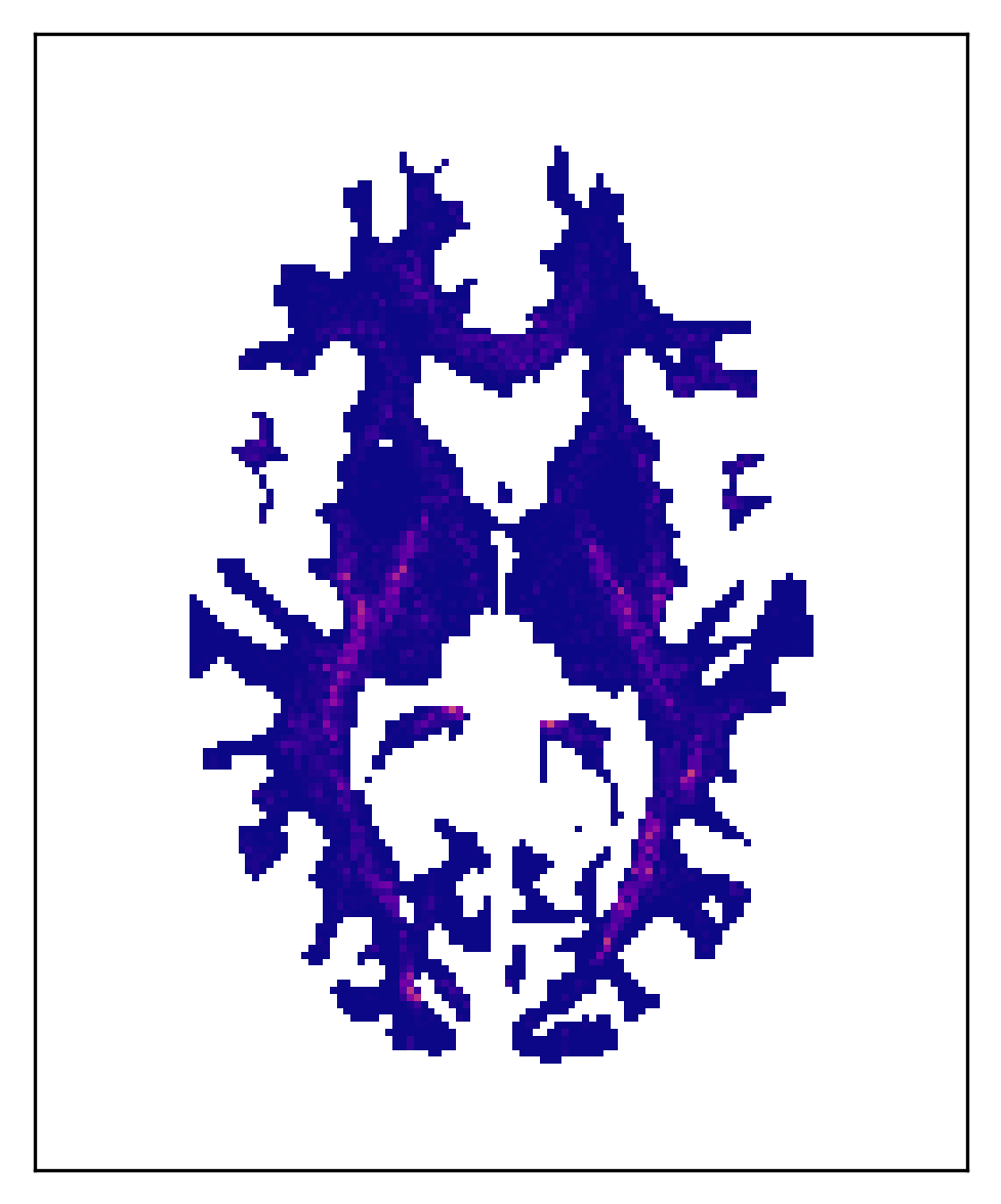

We performed a second experiment using the same tracking parameters, but seeding only in a single voxel at a time. For each voxel in the white matter we generated two tractographies (one train set, one test set), seeding only in that voxel 100 times. We then computed the cross-entropy between the two tractographies as a function of the number of samples in the training set. In Figure 3 we plot the marginal change in entropy over the white matter mask for one subject, both at the start of the process and the end.
For many regions the sampling process converges very quickly. However, for certain regions the sampling process converges quite slowly (albeit without considering samples from other voxels). This suggests at surface level high variance in complexity of the white matter when aggregating into voxels. Further, this provides evidence that a weighted seeding scheme might be more efficient than gridded or uniformly random schema.
4 Discussion
Our results suggest that in general the number of tracts required to closely approximate the underlying distribution is low using the methods we tested here. This can only be reduced by conditioning tracts or seeds on specific anatomic priors (e.g., seeding only in the corpus callosum or in a specific region). Further, the Human Connectome Project [22] data are widely regarded as examples of the state of the art. Other sources most likely have less signal content, leading to sharper (more steep) curves and even faster convergence.
On the other hand, this method is inherently limited: we cannot differentiate between “valid” signal and spurious systemic error. By sampling to the scales described in this paper researchers can accurately recover the streamline distribution (up to the chosen spatial scale). If this distribution includes “false” modes, i.e. modes that not from a corresponding biophysical structure, we will consistently recover those false modes. Larger sample sizes in simulations do nothing to guard against false signal; indeed, they reinforce them.
However, spurious random tracts that are not signal (i.e., caused by noise and not artifacts) will have vanishing weight. According to our empirical assessment, this will on average happen rapidly, relative to the weight of the modes.
Consider a tractography method that when queried ten times generates complete noise555the definition of complete noise is actually tricky, but we could use a proxy of “drawing a tract length uniformly at random between 1 and the number of voxels, and filling its sequence with points drawn uniformly from the domain of the image”. nine times and generates a real tract one time on average. Clearly this method has high noise ( useless!) and would not do well in major tractography challenges (e.g., [14]), but, we claim, this hypothetical method would still have value. Since the number of real tracts is finite and the number of possible noise tracts is comparatively large, increasing the sample size will lead to each real tract having more corresponding samples than the noise tracts. Given enough time we may recover the set of real tracts (which we then can simplify to save disk space).
Further consider a tractography method that when queried ten times generates complete noise eight times, generates a real tract one time, and generates a false but non-random tract the remaining time on average. Like the first hypothetical method, this second method produces useless tracts. However, increasing sample size will not lead to vanishing error in this second case due to the false mode (the non-random false tract).
Clearly, no method is purely in the first case; all methods likely have false modes. However, we posit that understanding the number, location, and size of these modes is just as important as understanding a method’s information efficiency (i.e., the proportion of true positives for fixed sample size). It is illustrative that F1-score is unable to differentiate between these two hypothetical methods. We believe such considerations should be taken into account, in that valuable methods might be slow to converge, and thus currently ignored.
5 Conclusion
In this paper we have investigated the empirical sample complexity of tractography distributions. We have provided a general methodology for estimating and comparing the information content of streamline methods, along with an example analysis of the Human Connectome Project dataset using four different tracking pipelines.
Acknowledgements
This work was supported by NIH Grant U54 EB020403 and DARPA grant W911NF-16-1-0575, as well as the NSF Graduate Research Fellowship Program.
References
- [1] Aganj, I., et al.: Reconstruction of the orientation distribution function in single-and multiple-shell q-ball imaging within constant solid angle. Magnetic Resonance in Medicine 64(2), 554–566 (2010)
- [2] Behrens, T.E., et al.: Probabilistic diffusion tractography with multiple fibre orientations: What can we gain? Neuroimage 34(1), 144–155 (2007)
- [3] Cheng, H., et al.: Optimization of seed density in dti tractography for structural networks. Journal of neuroscience methods 203(1), 264–272 (2012)
- [4] Coifman, R.R., Lafon, S.: Diffusion maps. Applied and computational harmonic analysis 21(1), 5–30 (2006)
- [5] Cover, T.M., Thomas, J.A.: Elements of information theory. Wiley & Sons (2012)
- [6] Fischl, B.: Freesurfer. NeuroImage 2(62), 774–781 (2012)
- [7] Garyfallidis, E.: Towards an accurate brain tractography. Ph.D. thesis, University of Cambridge (2013)
- [8] Garyfallidis, E., et al.: Quickbundles, a method for tractography simplification. Frontiers in neuroscience 6, 175 (2012)
- [9] Garyfallidis, E., et al.: Dipy, a library for the analysis of diffusion MRI data. Front. Neuroinform 8(8) (2014)
- [10] Garyfallidis, E., et al.: Recognition of white matter bundles using local and global streamline-based registration and clustering. NeuroImage (2017)
- [11] Girard, G., et al.: Towards quantitative connectivity analysis: reducing tractography biases. Neuroimage 98, 266–278 (2014)
- [12] Jordan, K.M., et al.: Cluster confidence index: A streamline-wise pathway reproducibility metric for diffusion-weighted mri tractography. Journal of Neuroimaging 28(1), 64–69 (2018)
- [13] Le Bihan, D., et al.: Diffusion tensor imaging: concepts and applications. Journal of magnetic resonance imaging 13(4), 534–546 (2001)
- [14] Maier-Hein, K.H., et al.: The challenge of mapping the human connectome based on diffusion tractography. Nature communications 8(1), 1349 (2017)
- [15] Miller, K.L., et al.: Multimodal population brain imaging in the uk biobank prospective epidemiological study. Nature neuroscience 19(11), 1523 (2016)
- [16] O’Donnell, L.J., Westin, C.F.: Automatic tractography segmentation using a high-dimensional white matter atlas. IEEE Trans on Med Imaging 26(11) (2007)
- [17] Prasad, G., Nir, T.M., Toga, A.W., Thompson, P.M.: Tractography density and network measures in alzheimer’s disease. In: Biomedical Imaging (ISBI), 2013 IEEE 10th International Symposium on. pp. 692–695. IEEE (2013)
- [18] Smith, R.E., et al.: SIFT2: Enabling dense quantitative assessment of brain white matter connectivity using streamlines tractography. Neuroimage 119 (2015)
- [19] Sotiropoulos, S.N., Zalesky, A.: Building connectomes using diffusion MRI: Why, how and but. NMR in Biomedicine (2017)
- [20] Thomas, C., et al.: Anatomical accuracy of brain connections derived from diffusion mri tractography is inherently limited. PNAS 111(46), 16574–16579 (2014)
- [21] Tournier, J.D., et al.: Resolving crossing fibres using constrained spherical deconvolution: validation using diffusion-weighted imaging phantom data. NeuroImage 42(2), 617–625 (2008)
- [22] Van Essen, D.C., et al.: The WU-Minn human connectome project: an overview. NeuroImage 80, 62–79 (2013)
- [23] Wassermann, D., et al.: Unsupervised white matter fiber clustering and tract probability map generation: Applications of a gaussian process framework for white matter fibers. NeuroImage 51(1), 228–241 (2010)
- [24] Zhang, Y., Brady, M., Smith, S.: Segmentation of brain MR images through a hidden Markov random field model and the expectation-maximization algorithm. IEEE Trans on Med Imaging 20(1), 45–57 (2001)