On the invariant manifolds of the fixed point of a second order nonlinear difference equation

Mehmet TURAN
Abstract

This paper addresses the asymptotic approximations of the stable and unstable manifolds for the saddle fixed point and the 2-periodic solutions of the difference equation xn+1=α+βxn1+xn1/xn,subscript𝑥𝑛1𝛼𝛽subscript𝑥𝑛1subscript𝑥𝑛1subscript𝑥𝑛x_{n+1}=\alpha+\beta x_{n-1}+x_{n-1}/x_{n}, where α>0,𝛼0\alpha>0, 0β<10𝛽10\leqslant\beta<1 and the initial conditions x1subscript𝑥1x_{-1} and x0subscript𝑥0x_{0} are positive numbers. These manifolds determine completely global dynamics of this equation. The theoretical results are supported by some numerical examples.

Keywords: Normal form, stable manifold, unstable manifold, center manifold.

2010 MSC: 39A10, 39A20, 37D10.

Atilim University, Department of Mathematics, Incek 06836, Ankara, Turkey
e-mail: mehmet.turan@atilim.edu.tr
Tel: +90 312 586 8585, Fax: +90 312 586 8091

1 Introduction

Many real world processes are studied by means of difference equations. Because of their wide range of applications in mechanics, economics, electronics, chemistry, ecology, biology, etc., the theory of discrete dynamical systems has been under intensive development and many researchers have been paying their attention to the study of these systems [1, 6, 7, 9, 10, 11, 12, 14, 16, 18].

The equation

xn+1=α+xn1xn,n=0,1,2,formulae-sequencesubscript𝑥𝑛1𝛼subscript𝑥𝑛1subscript𝑥𝑛𝑛012\displaystyle x_{n+1}=\alpha+\frac{x_{n-1}}{x_{n}},\qquad n=0,1,2,\ldots (1)

was investigated by many researchers. The equation (1), for α[0,)𝛼0\alpha\in[0,\infty) and the initial conditions x1subscript𝑥1x_{-1} and x0subscript𝑥0x_{0} being arbitrary positive real numbers, has been considered in [3]. There, the authors analyzed the global stability, the boundedness character, and the periodic nature of the positive solutions of (1). The global stability, the permanence, and the oscillation character of the recursive equation (1) for nonnegative values of the parameter α𝛼\alpha with negative initial conditions x1subscript𝑥1x_{-1} and x0subscript𝑥0x_{0} was investigated in [8]. The same equation for α<0𝛼0\alpha<0 was taken into account in [17]. The global bifurcation result for (1) was obtained in [4] and the asymptotic approximations of the stable and unstable manifolds of the fixed point of (1) were discussed in [13].

In this work, we consider the difference equation

xn+1=α+βxn1+xn1xn,n=0,1,2,formulae-sequencesubscript𝑥𝑛1𝛼𝛽subscript𝑥𝑛1subscript𝑥𝑛1subscript𝑥𝑛𝑛012\displaystyle x_{n+1}=\alpha+\beta x_{n-1}+\frac{x_{n-1}}{x_{n}},\qquad n=0,1,2,\ldots (2)

where α0,𝛼0\alpha\geqslant 0, 0β<1,0𝛽10\leqslant\beta<1, and the initial conditions x1subscript𝑥1x_{-1} and x0subscript𝑥0x_{0} are positive real numbers. Clearly, when β=0,𝛽0\beta=0, the equation (2) reduces to (1). For this reason, the results obtained in the current paper covers those given in [13].

Equation (2) has the unique fixed point

x¯=1+α1β.¯𝑥1𝛼1𝛽\displaystyle\bar{x}=\frac{1+\alpha}{1-\beta}. (3)

Letting yn=xn1subscript𝑦𝑛subscript𝑥𝑛1y_{n}=x_{n-1} and zn=xn,subscript𝑧𝑛subscript𝑥𝑛z_{n}=x_{n}, (2) can be written as

yn+1=znzn+1=α+βyn+ynznsubscript𝑦𝑛1subscript𝑧𝑛subscript𝑧𝑛1𝛼𝛽subscript𝑦𝑛subscript𝑦𝑛subscript𝑧𝑛\displaystyle\begin{array}[]{l}y_{n+1}=z_{n}\\ z_{n+1}=\alpha+\beta y_{n}+\displaystyle\frac{y_{n}}{z_{n}}\end{array} (6)

together with the initial conditions y0=x1,subscript𝑦0subscript𝑥1y_{0}=x_{-1}, z0=x0.subscript𝑧0subscript𝑥0z_{0}=x_{0}. Introducing the mapping

T(yz)=(zα+βy+yz),𝑇matrix𝑦𝑧matrix𝑧𝛼𝛽𝑦𝑦𝑧\displaystyle T\begin{pmatrix}y\\ z\end{pmatrix}=\begin{pmatrix}z\\ \alpha+\beta y+\displaystyle\frac{y}{z}\end{pmatrix}, (7)

(6) is written as

(yn+1zn+1)=T(ynzn).matrixsubscript𝑦𝑛1subscript𝑧𝑛1𝑇matrixsubscript𝑦𝑛subscript𝑧𝑛\displaystyle\begin{pmatrix}y_{n+1}\\ z_{n+1}\end{pmatrix}=T\begin{pmatrix}y_{n}\\ z_{n}\end{pmatrix}.

T𝑇T has a unique fixed point (x¯,x¯)¯𝑥¯𝑥(\bar{x},\bar{x}) where x¯¯𝑥\bar{x} is given by (3).

The following result for (2) was given in [2]:

Theorem 1.1

Let 0β<1.0𝛽10\leqslant\beta<1. For the equation (2), one has:

  • If 0α<1,0𝛼10\leqslant\alpha<1, the equilibrium point x¯¯𝑥\bar{x} is unstable;

  • If α=1,𝛼1\alpha=1, then there exists periodic solutions with period 2. Moreover, any non periodic solution of (2) converges either to the fixed point or to a two-periodic solution;

  • If α>1,𝛼1\alpha>1, then the equilibrium point x¯¯𝑥\bar{x} is globally asymptotically stable.

To complete the global dynamics of (2), the present paper addresses the equations of stable and unstable manifolds of the equilibrium solution and the stable manifold of period-two solutions of (2). The following definition of the stable and unstable manifolds and the next theorem about their existence can be found in [7, Definition 15.18, Theorem 15.19, pp.457] and also in [15]. We present these only with a minor change in notations for the convenience of the present paper.

Definition 1.2

Let 𝒩𝒩{\mathcal{N}} be a neighborhood of a fixed point x¯¯𝑥\bar{x} of a diffeomorphism T𝑇T defined in 𝒩.𝒩{\mathcal{N}}. Then, the local stable manifold Ws(x¯,𝒩),superscript𝑊𝑠¯𝑥𝒩W^{s}(\bar{x},{\mathcal{N}}), and the local unstable manifold Wu(x¯,𝒩)superscript𝑊𝑢¯𝑥𝒩W^{u}(\bar{x},{\mathcal{N}}) of x¯¯𝑥\bar{x} are defined, respectively, to be the following subsets of 𝒩::𝒩absent{\mathcal{N}}:

Ws(x¯,𝒩)={𝐱𝒩:Tn(𝐱)𝒩,for all n0,andTn(𝐱)x¯,asn}superscript𝑊𝑠¯𝑥𝒩conditional-set𝐱𝒩formulae-sequencesuperscript𝑇𝑛𝐱𝒩formulae-sequencefor all 𝑛0formulae-sequenceandsuperscript𝑇𝑛𝐱¯𝑥as𝑛\displaystyle W^{s}(\bar{x},{\mathcal{N}})=\{{\bf x}\in{\mathcal{N}}:T^{n}({\bf x})\in{\mathcal{N}},\ \text{for all }\ n\geqslant 0,\ \text{and}\ T^{n}({\bf x})\to\bar{x},\ \text{as}\ n\to\infty\}
Wu(x¯,𝒩)={𝐱𝒩:Tn(𝐱)𝒩,for all n0,andTn(𝐱)x¯,asn}superscript𝑊𝑢¯𝑥𝒩conditional-set𝐱𝒩formulae-sequencesuperscript𝑇𝑛𝐱𝒩formulae-sequencefor all 𝑛0formulae-sequenceandsuperscript𝑇𝑛𝐱¯𝑥as𝑛\displaystyle W^{u}(\bar{x},{\mathcal{N}})=\{{\bf x}\in{\mathcal{N}}:T^{-n}({\bf x})\in{\mathcal{N}},\ \text{for all }\ n\geqslant 0,\ \text{and}\ T^{-n}({\bf x})\to\bar{x},\ \text{as}\ n\to\infty\}
Theorem 1.3 (Stable and Unstable Manifolds)

Let T𝑇T be be a diffeomorphism with a hyperbolic saddle point x¯,¯𝑥\bar{x}, that is, the linearized map DT(x¯)𝐷𝑇¯𝑥DT(\bar{x}) at the fixed point has nonzero eigenvalues |λ1|<1subscript𝜆11|\lambda_{1}|<1 and |λ2|>1.subscript𝜆21|\lambda_{2}|>1. Then Ws(x¯,𝒩)superscript𝑊𝑠¯𝑥𝒩W^{s}(\bar{x},{\mathcal{N}}) is a curve tangent at x¯¯𝑥\bar{x} to, and a graph over, the eigenspace corresponding to λ1,subscript𝜆1\lambda_{1}, while Wu(x¯,𝒩)superscript𝑊𝑢¯𝑥𝒩W^{u}(\bar{x},{\mathcal{N}}) is a curve tangent at x¯¯𝑥\bar{x} to, and a graph over, the eigenspace corresponding to λ2subscript𝜆2\lambda_{2}. These curves are as smooth as the map T.𝑇T.

For the following theorem see [5, Theorem 6, pp 34].

Theorem 1.4 (Center Manifold)

Let T:n+mn+m:𝑇superscript𝑛𝑚superscript𝑛𝑚T:{\mathbb{R}}^{n+m}\to{\mathbb{R}}^{n+m} have the following form:

T(x,y)=(Ax+f(x,y),Bx+g(x,y))𝑇𝑥𝑦𝐴𝑥𝑓𝑥𝑦𝐵𝑥𝑔𝑥𝑦T(x,y)=(Ax+f(x,y),\ Bx+g(x,y))

where xn,𝑥superscript𝑛x\in{\mathbb{R}}^{n}, ym,𝑦superscript𝑚y\in{\mathbb{R}}^{m}, A𝐴A and B𝐵B are square matrices such that each eigenvalue of A𝐴A has modulus 1 and each eigenvalue of B𝐵B has modulus less than 1, f𝑓f and g𝑔g are C2superscript𝐶2C^{2} and f,g𝑓𝑔f,g and their first order derivatives are zero at the origin. Then, there exists a center manifold h:nm:superscript𝑛superscript𝑚h:{\mathbb{R}}^{n}\to{\mathbb{R}}^{m} for T.𝑇T. More precisely, for some ε>0𝜀0\varepsilon>0 there exists a C2superscript𝐶2C^{2} function h:nm:superscript𝑛superscript𝑚h:{\mathbb{R}}^{n}\to{\mathbb{R}}^{m} with h(0)=h(0)=00superscript00h(0)=h^{\prime}(0)=0 such that |x|<ε𝑥𝜀|x|<\varepsilon and (x1,y1)=T(x,h(x))subscript𝑥1subscript𝑦1𝑇𝑥𝑥(x_{1},y_{1})=T(x,h(x)) implies y1=h(x1).subscript𝑦1subscript𝑥1y_{1}=h(x_{1}).

The paper is organized as follows: In the next chapter, the normal form of the map T𝑇T and the equations of unstable and stable manifolds of the equilibrium solution are given. Chapter 3 deals with the normal form and invariant manifolds of the map T2.superscript𝑇2T^{2}. Finally, Chapter 4 is devoted to some numerical examples to illustrate the theoretical results.

2 Normal form and invariant manifolds of the map T𝑇T

2.1 Normal Form

To obtain the normal form of the map T,𝑇T, first, we transform its fixed point to the origin. For this, let un=ynx¯subscript𝑢𝑛subscript𝑦𝑛¯𝑥u_{n}=y_{n}-\bar{x} and vn=znx¯.subscript𝑣𝑛subscript𝑧𝑛¯𝑥v_{n}=z_{n}-\bar{x}. Then, (6) becomes

un+1=vnvn+1=βun+unvnvn+x¯.subscript𝑢𝑛1subscript𝑣𝑛subscript𝑣𝑛1𝛽subscript𝑢𝑛subscript𝑢𝑛subscript𝑣𝑛subscript𝑣𝑛¯𝑥\displaystyle\begin{array}[]{l}u_{n+1}=v_{n}\\ v_{n+1}=\beta u_{n}+\displaystyle\frac{u_{n}-v_{n}}{v_{n}+\bar{x}}\end{array}. (10)

For the mapping

F(uv)=(vβu+uvv+x¯),𝐹matrix𝑢𝑣matrix𝑣𝛽𝑢𝑢𝑣𝑣¯𝑥\displaystyle F\begin{pmatrix}u\\ v\end{pmatrix}=\begin{pmatrix}v\\ \beta u+\frac{u-v}{v+\bar{x}}\end{pmatrix},

(10) is written as

(un+1vn+1)=F(unvn).matrixsubscript𝑢𝑛1subscript𝑣𝑛1𝐹matrixsubscript𝑢𝑛subscript𝑣𝑛\displaystyle\begin{pmatrix}u_{n+1}\\ v_{n+1}\end{pmatrix}=F\begin{pmatrix}u_{n}\\ v_{n}\end{pmatrix}.

The Jacobian matrix of F𝐹F at its unique fixed point (0,0)00(0,0) is

J=(01β+1x¯1x¯)𝐽matrix01𝛽1¯𝑥1¯𝑥\displaystyle J=\begin{pmatrix}0&1\\ \beta+\frac{1}{\bar{x}}&-\frac{1}{\bar{x}}\end{pmatrix}

which has the eigenvalues

λ1=1θ2x¯andλ2=1+θ2x¯formulae-sequencesubscript𝜆11𝜃2¯𝑥andsubscript𝜆21𝜃2¯𝑥\displaystyle\lambda_{1}=\frac{-1-\theta}{2\bar{x}}\quad\text{and}\quad\lambda_{2}=\frac{-1+\theta}{2\bar{x}} (11)

with the corresponding eigenvectors

𝐯1=(2x¯1+θ,  1)Tand𝐯2=(2x¯1θ,  1)Tformulae-sequencesubscript𝐯1superscript2¯𝑥1𝜃1𝑇andsubscript𝐯2superscript2¯𝑥1𝜃1𝑇\displaystyle{\bf v}_{1}=\left(\frac{-2\bar{x}}{1+\theta}\>,\>\>1\right)^{T}\quad\text{and}\quad{\bf v}_{2}=\left(\frac{-2\bar{x}}{1-\theta}\>,\>\>1\right)^{T} (12)

respectively, where θ=1+4x¯+4βx¯2.𝜃14¯𝑥4𝛽superscript¯𝑥2\theta=\sqrt{1+4\bar{x}+4\beta\bar{x}^{2}}. Thus,

F(uv)=J(uv)+H(uv)𝐹matrix𝑢𝑣𝐽matrix𝑢𝑣𝐻matrix𝑢𝑣\displaystyle F\begin{pmatrix}u\\ v\end{pmatrix}=J\cdot\begin{pmatrix}u\\ v\end{pmatrix}+H\begin{pmatrix}u\\ v\end{pmatrix}

where

H(uv)=(0v(vu)x¯(v+x¯)).𝐻matrix𝑢𝑣matrix0𝑣𝑣𝑢¯𝑥𝑣¯𝑥\displaystyle H\begin{pmatrix}u\\ v\end{pmatrix}=\begin{pmatrix}0\\ \frac{v(v-u)}{\bar{x}(v+\bar{x})}\end{pmatrix}.

Thus, (6) is equivalent to

(un+1vn+1)=(01β+1x¯1x¯)(unvn)+H(unvn).matrixsubscript𝑢𝑛1subscript𝑣𝑛1matrix01𝛽1¯𝑥1¯𝑥matrixsubscript𝑢𝑛subscript𝑣𝑛𝐻matrixsubscript𝑢𝑛subscript𝑣𝑛\displaystyle\begin{pmatrix}u_{n+1}\\ v_{n+1}\end{pmatrix}=\begin{pmatrix}0&1\\ \beta+\frac{1}{\bar{x}}&-\frac{1}{\bar{x}}\end{pmatrix}\begin{pmatrix}u_{n}\\ v_{n}\end{pmatrix}+H\begin{pmatrix}u_{n}\\ v_{n}\end{pmatrix}. (13)

Set P=(𝐯1𝐯2),𝑃subscript𝐯1subscript𝐯2P=({\bf v}_{1}\>{\bf v}_{2}), where 𝐯1subscript𝐯1{\bf v}_{1} and 𝐯2subscript𝐯2{\bf v}_{2} are given by (12), and let

(unvn)=P(ξnηn).matrixsubscript𝑢𝑛subscript𝑣𝑛𝑃matrixsubscript𝜉𝑛subscript𝜂𝑛\displaystyle\begin{pmatrix}u_{n}\\ v_{n}\end{pmatrix}=P\cdot\begin{pmatrix}\xi_{n}\\ \eta_{n}\end{pmatrix}. (14)

Then, (13) becomes

(ξn+1ηn+1)=(λ100λ2)(ξnηn)+(f(ξn,ηn)g(ξn,ηn))matrixsubscript𝜉𝑛1subscript𝜂𝑛1matrixsubscript𝜆100subscript𝜆2matrixsubscript𝜉𝑛subscript𝜂𝑛matrix𝑓subscript𝜉𝑛subscript𝜂𝑛𝑔subscript𝜉𝑛subscript𝜂𝑛\displaystyle\begin{pmatrix}\xi_{n+1}\\ \eta_{n+1}\end{pmatrix}=\begin{pmatrix}\lambda_{1}&0\\ 0&\lambda_{2}\end{pmatrix}\begin{pmatrix}\xi_{n}\\ \eta_{n}\end{pmatrix}+\begin{pmatrix}f(\xi_{n},\eta_{n})\\ g(\xi_{n},\eta_{n})\end{pmatrix} (15)

where

f(ξ,η)=(1+2βx¯)(ξ+η)2+θ(ξ2η2)θ(θ1)(ξ+η+x¯),g(ξ,η)=(1+2βx¯)(ξ+η)2+θ(ξ2η2)θ(θ+1)(ξ+η+x¯).𝑓𝜉𝜂12𝛽¯𝑥superscript𝜉𝜂2𝜃superscript𝜉2superscript𝜂2𝜃𝜃1𝜉𝜂¯𝑥𝑔𝜉𝜂12𝛽¯𝑥superscript𝜉𝜂2𝜃superscript𝜉2superscript𝜂2𝜃𝜃1𝜉𝜂¯𝑥\displaystyle\begin{array}[]{l}f(\xi,\eta)=\displaystyle\frac{(1+2\beta\bar{x})(\xi+\eta)^{2}+\theta(\xi^{2}-\eta^{2})}{\theta(\theta-1)(\xi+\eta+\bar{x})},\\ g(\xi,\eta)=\displaystyle\frac{(1+2\beta\bar{x})(\xi+\eta)^{2}+\theta(\xi^{2}-\eta^{2})}{\theta(\theta+1)(\xi+\eta+\bar{x})}.\end{array} (18)

System (15) is called the normal form of (6).

2.2 Unstable manifold of the equilibrium solution

Let 0<α<1.0𝛼10<\alpha<1. Then, as it is stated in [2], the fixed point x¯¯𝑥\bar{x} of (2) is unstable. In fact, it can be shown that |λ1|>1subscript𝜆11|\lambda_{1}|>1 and |λ2|<1.subscript𝜆21|\lambda_{2}|<1. Then, by Theorem 1.3, there is an unstable manifold Wusuperscript𝑊𝑢W^{u} which is the graph of an analytic map φ:E1E2:𝜑subscript𝐸1subscript𝐸2\varphi:E_{1}\to E_{2} such that φ(0)=φ(0)=0.𝜑0superscript𝜑00\varphi(0)=\varphi^{\prime}(0)=0. Let

φ(ξ)=a2ξ2+a3ξ3+O(ξ4),a2,a3.formulae-sequence𝜑𝜉subscript𝑎2superscript𝜉2subscript𝑎3superscript𝜉3𝑂superscript𝜉4subscript𝑎2subscript𝑎3\varphi(\xi)=a_{2}\xi^{2}+a_{3}\xi^{3}+O(\xi^{4}),\quad a_{2},a_{3}\in{\mathbb{R}}.

Now, we shall compute a2subscript𝑎2a_{2} and a3.subscript𝑎3a_{3}. On the manifold Wu,superscript𝑊𝑢W^{u}, we have ηn=φ(ξn)subscript𝜂𝑛𝜑subscript𝜉𝑛\eta_{n}=\varphi(\xi_{n}) for n0.𝑛subscript0n\in{\mathbb{N}}_{0}. Thus, the function φ𝜑\varphi must satisfy

φ(λ1ξ+f(ξ,φ(ξ)))=λ2φ(ξ)+g(ξ,φ(ξ))𝜑subscript𝜆1𝜉𝑓𝜉𝜑𝜉subscript𝜆2𝜑𝜉𝑔𝜉𝜑𝜉\displaystyle\varphi(\lambda_{1}\xi+f(\xi,\varphi(\xi)))=\lambda_{2}\varphi(\xi)+g(\xi,\varphi(\xi)) (19)

where f𝑓f and g𝑔g are given in (18). Rewriting (19) as a polynomial equation in ξ𝜉\xi and equation the coefficients of ξ2superscript𝜉2\xi^{2} and ξ3superscript𝜉3\xi^{3} to 0, we obtain

a2=1+θ+2βx¯θ(θ+1)(λ12λ2)x¯subscript𝑎21𝜃2𝛽¯𝑥𝜃𝜃1superscriptsubscript𝜆12subscript𝜆2¯𝑥\displaystyle a_{2}=\frac{1+\theta+2\beta\bar{x}}{\theta(\theta+1)(\lambda_{1}^{2}-\lambda_{2})\bar{x}} (20)

and

a3=a2(λ13λ2)x¯[λ2λ121+2βx¯θx¯(1λ1+λ1λ2)λ1λ2x¯].subscript𝑎3subscript𝑎2superscriptsubscript𝜆13subscript𝜆2¯𝑥delimited-[]subscript𝜆2superscriptsubscript𝜆1212𝛽¯𝑥𝜃¯𝑥1subscript𝜆1subscript𝜆1subscript𝜆2subscript𝜆1subscript𝜆2¯𝑥\displaystyle a_{3}=\frac{a_{2}}{(\lambda_{1}^{3}-\lambda_{2})\bar{x}}\left[\lambda_{2}-\lambda_{1}^{2}-\frac{1+2\beta\bar{x}}{\theta\bar{x}}\left(\frac{1}{\lambda_{1}}+\frac{\lambda_{1}}{\lambda_{2}}\right)-\frac{\lambda_{1}}{\lambda_{2}\bar{x}}\right]. (21)

The local unstable manifold is obtained locally as the graph of the map φ(ξ)=a2ξ2+a3ξ3.𝜑𝜉subscript𝑎2superscript𝜉2subscript𝑎3superscript𝜉3\varphi(\xi)=a_{2}\xi^{2}+a_{3}\xi^{3}. Since ηn=a2ξn2+a3ξn3,subscript𝜂𝑛subscript𝑎2superscriptsubscript𝜉𝑛2subscript𝑎3superscriptsubscript𝜉𝑛3\eta_{n}=a_{2}\xi_{n}^{2}+a_{3}\xi_{n}^{3}, using (14) and un=xn1x¯,subscript𝑢𝑛subscript𝑥𝑛1¯𝑥u_{n}=x_{n-1}-\bar{x}, vn=xnx¯,subscript𝑣𝑛subscript𝑥𝑛¯𝑥v_{n}=x_{n}-\bar{x}, we can approximate locally the local unstable manifold Wlocusuperscriptsubscript𝑊𝑙𝑜𝑐𝑢W_{loc}^{u} of (2) as the graph of φ~(x)~𝜑𝑥\tilde{\varphi}(x) such that U(x,φ~(x))=0𝑈𝑥~𝜑𝑥0U(x,\tilde{\varphi}(x))=0 where

U(x,y):=γ1(xx¯)γ2(yx¯)+a2[γ1(xx¯)+γ3(yx¯)]2+a3[γ1(xx¯)+γ3(yx¯)]3assign𝑈𝑥𝑦subscript𝛾1𝑥¯𝑥subscript𝛾2𝑦¯𝑥subscript𝑎2superscriptdelimited-[]subscript𝛾1𝑥¯𝑥subscript𝛾3𝑦¯𝑥2subscript𝑎3superscriptdelimited-[]subscript𝛾1𝑥¯𝑥subscript𝛾3𝑦¯𝑥3\displaystyle U(x,y):=\gamma_{1}(x-\bar{x})-\gamma_{2}(y-\bar{x})+a_{2}\left[\gamma_{1}(x-\bar{x})+\gamma_{3}(y-\bar{x})\right]^{2}+a_{3}\left[\gamma_{1}(x-\bar{x})+\gamma_{3}(y-\bar{x})\right]^{3} (22)

in which

γ1=1+βx¯θ,γ2=θ12θandγ3=θ+12θ.formulae-sequencesubscript𝛾11𝛽¯𝑥𝜃formulae-sequencesubscript𝛾2𝜃12𝜃andsubscript𝛾3𝜃12𝜃\displaystyle\gamma_{1}=\frac{1+\beta\bar{x}}{-\theta},\quad\gamma_{2}=\frac{\theta-1}{2\theta}\quad\text{and}\quad\gamma_{3}=\frac{\theta+1}{2\theta}. (23)

It is easy to see that the function φ~(x)~𝜑𝑥\tilde{\varphi}(x) satisfies

φ~(x¯)=x¯andφ~(x¯)=1+θ2x¯.formulae-sequence~𝜑¯𝑥¯𝑥andsuperscript~𝜑¯𝑥1𝜃2¯𝑥\displaystyle\tilde{\varphi}(\bar{x})=\bar{x}\quad\textnormal{and}\quad\tilde{\varphi}^{\prime}(\bar{x})=-\frac{1+\theta}{2\bar{x}}.

Thus, we have proved the following theorem:

Theorem 2.1

The local unstable manifold of (2) corresponding to the saddle point x¯¯𝑥\bar{x} has the asymptotic equation U(x,φ~(x))=0𝑈𝑥~𝜑𝑥0U(x,\tilde{\varphi}(x))=0 where U(x,y)𝑈𝑥𝑦U(x,y) is given by (22).

2.3 Stable manifold of the equilibrium solution

Since |λ1|>1subscript𝜆11|\lambda_{1}|>1 and |λ2|<1,subscript𝜆21|\lambda_{2}|<1, by Theorem 1.3, there is a stable manifold Wssuperscript𝑊𝑠W^{s} which is the graph of an analytic map ψ:E1E2:𝜓subscript𝐸1subscript𝐸2\psi:E_{1}\to E_{2} such that ψ(0)=ψ(0)=0.𝜓0superscript𝜓00\psi(0)=\psi^{\prime}(0)=0. Let

ψ(η)=b2η2+b3η3+O(η4),b2,b3.formulae-sequence𝜓𝜂subscript𝑏2superscript𝜂2subscript𝑏3superscript𝜂3𝑂superscript𝜂4subscript𝑏2subscript𝑏3\psi(\eta)=b_{2}\eta^{2}+b_{3}\eta^{3}+O(\eta^{4}),\quad b_{2},b_{3}\in{\mathbb{R}}.

Now, we shall compute the coefficients b2subscript𝑏2b_{2} and b3.subscript𝑏3b_{3}. On the manifold Ws,superscript𝑊𝑠W^{s}, we have ξn=ψ(ηn)subscript𝜉𝑛𝜓subscript𝜂𝑛\xi_{n}=\psi(\eta_{n}) for n0.𝑛subscript0n\in{\mathbb{N}}_{0}. Thus, the function ψ𝜓\psi must satisfy

ψ(λ2η+g(ψ(η),η))=λ1ψ(η)+f(ψ(η),η)𝜓subscript𝜆2𝜂𝑔𝜓𝜂𝜂subscript𝜆1𝜓𝜂𝑓𝜓𝜂𝜂\displaystyle\psi(\lambda_{2}\eta+g(\psi(\eta),\eta))=\lambda_{1}\psi(\eta)+f(\psi(\eta),\eta) (24)

where f𝑓f and g𝑔g are given in (18). Rewriting (24) as a polynomial equation in η𝜂\eta and equating the coefficients of η2superscript𝜂2\eta^{2} and η3superscript𝜂3\eta^{3} to 0, we obtain

b2=1θ+2βx¯θ(θ1)(λ22λ1)x¯subscript𝑏21𝜃2𝛽¯𝑥𝜃𝜃1superscriptsubscript𝜆22subscript𝜆1¯𝑥\displaystyle b_{2}=\frac{1-\theta+2\beta\bar{x}}{\theta(\theta-1)(\lambda_{2}^{2}-\lambda_{1})\bar{x}} (25)

and

b3=b2(λb3λ1)x¯[λ1λ22+1+2βx¯θx¯(1λ2+λ2λ1)λ2λ1x¯].subscript𝑏3subscript𝑏2superscriptsubscript𝜆𝑏3subscript𝜆1¯𝑥delimited-[]subscript𝜆1superscriptsubscript𝜆2212𝛽¯𝑥𝜃¯𝑥1subscript𝜆2subscript𝜆2subscript𝜆1subscript𝜆2subscript𝜆1¯𝑥\displaystyle b_{3}=\frac{b_{2}}{(\lambda_{b}^{3}-\lambda_{1})\bar{x}}\left[\lambda_{1}-\lambda_{2}^{2}+\frac{1+2\beta\bar{x}}{\theta\bar{x}}\left(\frac{1}{\lambda_{2}}+\frac{\lambda_{2}}{\lambda_{1}}\right)-\frac{\lambda_{2}}{\lambda_{1}\bar{x}}\right]. (26)

The local stable manifold is obtained locally as the graph of the map ψ(η)=b2η2+b3η3.𝜓𝜂subscript𝑏2superscript𝜂2subscript𝑏3superscript𝜂3\psi(\eta)=b_{2}\eta^{2}+b_{3}\eta^{3}. Since ξn=b2ηn2+b3ηn3,subscript𝜉𝑛subscript𝑏2superscriptsubscript𝜂𝑛2subscript𝑏3superscriptsubscript𝜂𝑛3\xi_{n}=b_{2}\eta_{n}^{2}+b_{3}\eta_{n}^{3}, using (14) and un=xn1x¯,subscript𝑢𝑛subscript𝑥𝑛1¯𝑥u_{n}=x_{n-1}-\bar{x}, vn=xnx¯,subscript𝑣𝑛subscript𝑥𝑛¯𝑥v_{n}=x_{n}-\bar{x}, we can approximate locally the local stable manifold Wlocssuperscriptsubscript𝑊𝑙𝑜𝑐𝑠W_{loc}^{s} of (2) as the graph of ψ~(y)~𝜓𝑦\tilde{\psi}(y) such that S(ψ~(y),y)=0𝑆~𝜓𝑦𝑦0S(\tilde{\psi}(y),y)=0 where

S(x,y):=γ1(xx¯)+γ3(yx¯)b2[γ1(xx¯)γ2(yx¯)]2+b3[γ1(xx¯)γ2(yx¯)]3.assign𝑆𝑥𝑦subscript𝛾1𝑥¯𝑥subscript𝛾3𝑦¯𝑥subscript𝑏2superscriptdelimited-[]subscript𝛾1𝑥¯𝑥subscript𝛾2𝑦¯𝑥2subscript𝑏3superscriptdelimited-[]subscript𝛾1𝑥¯𝑥subscript𝛾2𝑦¯𝑥3\displaystyle S(x,y):=\gamma_{1}(x-\bar{x})+\gamma_{3}(y-\bar{x})-b_{2}\left[\gamma_{1}(x-\bar{x})-\gamma_{2}(y-\bar{x})\right]^{2}+b_{3}\left[\gamma_{1}(x-\bar{x})-\gamma_{2}(y-\bar{x})\right]^{3}. (27)

It is easy to see that the function ψ~(x)~𝜓𝑥\tilde{\psi}(x) satisfies

ψ~(x¯)=x¯andψ~(x¯)=2x¯θ1.formulae-sequence~𝜓¯𝑥¯𝑥andsuperscript~𝜓¯𝑥2¯𝑥𝜃1\displaystyle\tilde{\psi}(\bar{x})=\bar{x}\quad\textnormal{and}\quad\tilde{\psi}^{\prime}(\bar{x})=\frac{2\bar{x}}{\theta-1}.

Thus, we have proved the following theorem:

Theorem 2.2

The local stable manifold of (2) corresponding to the saddle point x¯¯𝑥\bar{x} has the asymptotic equation S(ψ~(y),y)=0𝑆~𝜓𝑦𝑦0S(\tilde{\psi}(y),y)=0 where S(x,y)𝑆𝑥𝑦S(x,y) is given by (27).

3 Normal form and invariant manifold of the map T2superscript𝑇2T^{2}

3.1 Normal Form

For the map T𝑇T given by (7), one has

T2(yz)=(1+βy+y/z1+βz+z1+βy+y/z).superscript𝑇2matrix𝑦𝑧matrix1𝛽𝑦𝑦𝑧1𝛽𝑧𝑧1𝛽𝑦𝑦𝑧\displaystyle T^{2}\begin{pmatrix}y\\ z\end{pmatrix}=\begin{pmatrix}1+\beta y+y/z\\ 1+\beta z+\frac{z}{1+\beta y+y/z}\end{pmatrix}. (28)

That is,

(yn+2zn+2)=T2(ynzn).matrixsubscript𝑦𝑛2subscript𝑧𝑛2superscript𝑇2matrixsubscript𝑦𝑛subscript𝑧𝑛\displaystyle\begin{pmatrix}y_{n+2}\\ z_{n+2}\end{pmatrix}=T^{2}\begin{pmatrix}y_{n}\\ z_{n}\end{pmatrix}. (29)

Firstly, we note that the fixed point (x¯,x¯)¯𝑥¯𝑥(\bar{x},\bar{x}) of T𝑇T is also a fixed point of T2.superscript𝑇2T^{2}. That is why, in this section, the fixed point (x¯,x¯)¯𝑥¯𝑥(\bar{x},\bar{x}) of T2superscript𝑇2T^{2} is ignored, and the main focus will be on the other fixed points. As it was shown in [2], when α=1,𝛼1\alpha=1, equation (2) has infinitely many 2-periodic solutions each of which corresponds to a fixed point of T2.superscript𝑇2T^{2}. Indeed, if Φ>1/(1β),Φ11𝛽\Phi>1/(1-\beta), then all the fixed points of T2superscript𝑇2T^{2} are given by (Φ,Ψ)ΦΨ(\Phi,\Psi) where Ψ=Φ/[(1β)Φ1]).\Psi=\Phi/[(1-\beta)\Phi-1]). It is worth mentioning that Ψ>1/(1β)Ψ11𝛽\Psi>1/(1-\beta) and for the initial conditions x1=Φsubscript𝑥1Φx_{-1}=\Phi and x0=Ψ,subscript𝑥0Ψx_{0}=\Psi, the solution of (2) is {Φ,Ψ,Φ,Ψ,}.ΦΨΦΨ\{\Phi,\Psi,\Phi,\Psi,\ldots\}. Swapping the initial values produces the periodic solution {Ψ,Φ,Ψ,Φ,}.ΨΦΨΦ\{\Psi,\Phi,\Psi,\Phi,\ldots\}.

As it was done in the previous section, the fixed point (Φ,Ψ)ΦΨ(\Phi,\Psi) will be transformed to the origin. For this, let u=yΦ𝑢𝑦Φu=y-\Phi and v=zΨ.𝑣𝑧Ψv=z-\Psi. Then, we get the map

F0(uv):=T2(u+Φv+Ψ)(ΦΨ)=(βu+u+Φv+ΨΦΨβv+(v+Ψ)2v+Ψ+(u+Φ)(1+βv+βΨ)ΨΦ),\displaystyle F_{0}\begin{pmatrix}u\\ v\end{pmatrix}:=T^{2}\begin{pmatrix}u+\Phi\\ v+\Psi\end{pmatrix}-\begin{pmatrix}\Phi\\ \Psi\end{pmatrix}=\begin{pmatrix}\beta u+\frac{u+\Phi}{v+\Psi}-\frac{\Phi}{\Psi}\\ \beta v+\frac{(v+\Psi)^{2}}{v+\Psi+(u+\Phi)(1+\beta v+\beta\Psi)}-\frac{\Psi}{\Phi}\end{pmatrix}, (30)

for which (29) can be written as

(un+2vn+2)=F0(unvn).matrixsubscript𝑢𝑛2subscript𝑣𝑛2subscript𝐹0matrixsubscript𝑢𝑛subscript𝑣𝑛\displaystyle\begin{pmatrix}u_{n+2}\\ v_{n+2}\end{pmatrix}=F_{0}\begin{pmatrix}u_{n}\\ v_{n}\end{pmatrix}. (31)

It is clear to see that (0,0)00(0,0) is a fixed point of F0subscript𝐹0F_{0} and the Jacobian of F0subscript𝐹0F_{0} at this fixed point is

J0=(β+1ΨΦΨ2βΨ+1Φ2β+1Φ+1ΨΦ).subscript𝐽0matrix𝛽1ΨΦsuperscriptΨ2𝛽Ψ1superscriptΦ2𝛽1Φ1ΨΦ\displaystyle J_{0}=\begin{pmatrix}\beta+\frac{1}{\Psi}&-\frac{\Phi}{\Psi^{2}}\\ -\frac{\beta\Psi+1}{\Phi^{2}}&\beta+\frac{1}{\Phi}+\frac{1}{\Psi\Phi}\end{pmatrix}. (32)

Using the relation 1Φ+1Ψ=1β,1Φ1Ψ1𝛽\frac{1}{\Phi}+\frac{1}{\Psi}=1-\beta, one can rewrite (32) as

J0=(11ΦΦΨ2Ψ(1Φ)Φ311Ψ+1ΨΦ).subscript𝐽0matrix11ΦΦsuperscriptΨ2Ψ1ΦsuperscriptΦ311Ψ1ΨΦ\displaystyle J_{0}=\begin{pmatrix}1-\frac{1}{\Phi}&-\frac{\Phi}{\Psi^{2}}\\ \frac{\Psi(1-\Phi)}{\Phi^{3}}&1-\frac{1}{\Psi}+\frac{1}{\Psi\Phi}\end{pmatrix}.

from which it can be derived that the eigenvalues of J0subscript𝐽0J_{0} are

λ01=(11Φ)(11Ψ)andλ02=1.formulae-sequencesubscript𝜆0111Φ11Ψandsubscript𝜆021\displaystyle\lambda_{01}=\left(1-\frac{1}{\Phi}\right)\left(1-\frac{1}{\Psi}\right)\quad\text{and}\quad\lambda_{02}=1.

Since 0<λ01<10subscript𝜆0110<\lambda_{01}<1 and λ02=1,subscript𝜆021\lambda_{02}=1, the fixed point (Φ,Ψ)ΦΨ(\Phi,\Psi) is stable. The eigenvectors corresponding to the eigenvalues λ01subscript𝜆01\lambda_{01} and λ02subscript𝜆02\lambda_{02} are

𝐯01=(Φ2(Φ1)Ψ,  1)Tand𝐯02=(Φ2Ψ2,  1)T,formulae-sequencesubscript𝐯01superscriptsuperscriptΦ2Φ1Ψ1𝑇andsubscript𝐯02superscriptsuperscriptΦ2superscriptΨ21𝑇\displaystyle{\bf v}_{01}=\left(\frac{\Phi^{2}}{(\Phi-1)\Psi}\>,\>\>1\right)^{T}\quad\text{and}\quad{\bf v}_{02}=\left(-\frac{\Phi^{2}}{\Psi^{2}}\>,\>\>1\right)^{T}, (33)

respectively. Thus, the map obtained in (30) can be written as

F0(uv)=J0(uv)+H0(uv)subscript𝐹0matrix𝑢𝑣subscript𝐽0matrix𝑢𝑣subscript𝐻0matrix𝑢𝑣\displaystyle F_{0}\begin{pmatrix}u\\ v\end{pmatrix}=J_{0}\cdot\begin{pmatrix}u\\ v\end{pmatrix}+H_{0}\begin{pmatrix}u\\ v\end{pmatrix} (34)

where

H0(uv)=(v(ΦvΨu)Ψ2(v+Ψ)(v+Ψ)2v+Ψ+(u+Φ)(1+βv+βΨ)+(βΨ+1)uΦ2(Ψ+1)vΨΦΨΦ).subscript𝐻0matrix𝑢𝑣matrix𝑣Φ𝑣Ψ𝑢superscriptΨ2𝑣Ψsuperscript𝑣Ψ2𝑣Ψ𝑢Φ1𝛽𝑣𝛽Ψ𝛽Ψ1𝑢superscriptΦ2Ψ1𝑣ΨΦΨΦ\displaystyle H_{0}\begin{pmatrix}u\\ v\end{pmatrix}=\begin{pmatrix}\frac{v(\Phi v-\Psi u)}{\Psi^{2}(v+\Psi)}\\ \frac{(v+\Psi)^{2}}{v+\Psi+(u+\Phi)(1+\beta v+\beta\Psi)}+\frac{(\beta\Psi+1)u}{\Phi^{2}}-\frac{(\Psi+1)v}{\Psi\Phi}-\frac{\Psi}{\Phi}\end{pmatrix}.

Therefore, (29) is equivalent to

(un+2vn+2)=(11ΦΦΨ2Ψ(1Φ)Φ311Ψ+1ΨΦ)(unvn)+H0(unvn).matrixsubscript𝑢𝑛2subscript𝑣𝑛2matrix11ΦΦsuperscriptΨ2Ψ1ΦsuperscriptΦ311Ψ1ΨΦmatrixsubscript𝑢𝑛subscript𝑣𝑛subscript𝐻0matrixsubscript𝑢𝑛subscript𝑣𝑛\displaystyle\begin{pmatrix}u_{n+2}\\ v_{n+2}\end{pmatrix}=\begin{pmatrix}1-\frac{1}{\Phi}&-\frac{\Phi}{\Psi^{2}}\\ \frac{\Psi(1-\Phi)}{\Phi^{3}}&1-\frac{1}{\Psi}+\frac{1}{\Psi\Phi}\end{pmatrix}\begin{pmatrix}u_{n}\\ v_{n}\end{pmatrix}+H_{0}\begin{pmatrix}u_{n}\\ v_{n}\end{pmatrix}. (35)

Set P0=(𝐯01𝐯02),subscript𝑃0subscript𝐯01subscript𝐯02P_{0}=({\bf v}_{01}\>{\bf v}_{02}), where 𝐯01subscript𝐯01{\bf v}_{01} and 𝐯02subscript𝐯02{\bf v}_{02} are given by (33), and let

(uv)=P0(ξη).matrix𝑢𝑣subscript𝑃0matrix𝜉𝜂\displaystyle\begin{pmatrix}u\\ v\end{pmatrix}=P_{0}\cdot\begin{pmatrix}\xi\\ \eta\end{pmatrix}. (36)

Then, (35) leads to

(ξn+2ηn+2)=(λ0100λ02)(ξnηn)+(f0(ξn,ηn)g0(ξn,ηn))matrixsubscript𝜉𝑛2subscript𝜂𝑛2matrixsubscript𝜆0100subscript𝜆02matrixsubscript𝜉𝑛subscript𝜂𝑛matrixsubscript𝑓0subscript𝜉𝑛subscript𝜂𝑛subscript𝑔0subscript𝜉𝑛subscript𝜂𝑛\displaystyle\begin{pmatrix}\xi_{n+2}\\ \eta_{n+2}\end{pmatrix}=\begin{pmatrix}\lambda_{01}&0\\ 0&\lambda_{02}\end{pmatrix}\begin{pmatrix}\xi_{n}\\ \eta_{n}\end{pmatrix}+\begin{pmatrix}f_{0}(\xi_{n},\eta_{n})\\ g_{0}(\xi_{n},\eta_{n})\end{pmatrix} (37)

where

f0(ξ,η)=Φ1Ψ+Φ1(ζξΦΨη(Φ+Ψ)Φ(ξ+η+Ψ)+(ξ+η)ξΦ(1Φ)(ξ+η+Ψ)),g0(ξ,η)=ΨΨ+Φ1(ζη(Φ+Ψ)ΦΨξΦ(ξ+η+Ψ)+(1Φ)(Φ+Ψ)(ξ+η)ηΦΨ2(ξ+η+Ψ)).subscript𝑓0𝜉𝜂Φ1ΨΦ1𝜁𝜉ΦΨ𝜂ΦΨΦ𝜉𝜂Ψ𝜉𝜂𝜉Φ1Φ𝜉𝜂Ψsubscript𝑔0𝜉𝜂ΨΨΦ1𝜁𝜂ΦΨΦΨ𝜉Φ𝜉𝜂Ψ1ΦΦΨ𝜉𝜂𝜂ΦsuperscriptΨ2𝜉𝜂Ψ\displaystyle\begin{array}[]{l}f_{0}(\xi,\eta)=\displaystyle\frac{\Phi-1}{\Psi+\Phi-1}\left(\zeta-\frac{\xi}{\Phi\Psi}-\frac{\eta(\Phi+\Psi)}{\Phi(\xi+\eta+\Psi)}+\frac{(\xi+\eta)\xi}{\Phi(1-\Phi)(\xi+\eta+\Psi)}\right),\\ g_{0}(\xi,\eta)=\displaystyle\frac{\Psi}{\Psi+\Phi-1}\left(\zeta-\frac{\eta(\Phi+\Psi)}{\Phi\Psi}-\frac{\xi}{\Phi(\xi+\eta+\Psi)}+\frac{(1-\Phi)(\Phi+\Psi)(\xi+\eta)\eta}{\Phi\Psi^{2}(\xi+\eta+\Psi)}\right).\end{array} (40)

and

ζ=(ξ+η+Ψ)2ξ+η+Ψ+(Φ2ξ(Φ1)ΨΦ2ηΨ2+Φ)(1+βξ+βη+βΨ)ΨΦ.𝜁superscript𝜉𝜂Ψ2𝜉𝜂ΨsuperscriptΦ2𝜉Φ1ΨsuperscriptΦ2𝜂superscriptΨ2Φ1𝛽𝜉𝛽𝜂𝛽ΨΨΦ\zeta=\frac{(\xi+\eta+\Psi)^{2}}{\xi+\eta+\Psi+\left(\frac{\Phi^{2}\xi}{(\Phi-1)\Psi}-\frac{\Phi^{2}\eta}{\Psi^{2}}+\Phi\right)(1+\beta\xi+\beta\eta+\beta\Psi)}-\frac{\Psi}{\Phi}.

System (37) is the normal of (29).

3.2 Stable set of 2-periodic solution {(Φ,Ψ),(Ψ,Φ)}ΦΨΨΦ\{(\Phi,\Psi),(\Psi,\Phi)\}

Since 0<λ01<10subscript𝜆0110<\lambda_{01}<1 and λ02=1,subscript𝜆021\lambda_{02}=1, by Theorem 1.4, there is an invariant curve 𝒞𝒞{\mathcal{C}} (called center manifold) which is the graph of an analytic map hh such that h(0)=h(0)=0.0superscript00h(0)=h^{\prime}(0)=0. Let

h(ξ)=c2ξ2+c3ξ3+O(ξ4),c2,c3.formulae-sequence𝜉subscript𝑐2superscript𝜉2subscript𝑐3superscript𝜉3𝑂superscript𝜉4subscript𝑐2subscript𝑐3\displaystyle h(\xi)=c_{2}\xi^{2}+c_{3}\xi^{3}+O(\xi^{4}),\quad c_{2},c_{3}\in{\mathbb{R}}.

Now, we shall compute c2subscript𝑐2c_{2} and c3.subscript𝑐3c_{3}. The function hh must satisfy

h(λ01ξ+f0(ξ,h(ξ)))=h(ξ)+g0(ξ,h(ξ))subscript𝜆01𝜉subscript𝑓0𝜉𝜉𝜉subscript𝑔0𝜉𝜉\displaystyle h(\lambda_{01}\xi+f_{0}(\xi,h(\xi)))=h(\xi)+g_{0}(\xi,h(\xi)) (41)

where λ01subscript𝜆01\lambda_{01} is given in (33), f0subscript𝑓0f_{0} and g0subscript𝑔0g_{0} are given in (40). Rewriting (41) as a polynomial equation in ξ𝜉\xi and equation the coefficients of ξ2superscript𝜉2\xi^{2} and ξ3superscript𝜉3\xi^{3} to 0, we obtain

c2=Φ(1Φ)(Φ+Ψ1)(2ΦΨΦΨ+1)subscript𝑐2Φ1ΦΦΨ12ΦΨΦΨ1\displaystyle c_{2}=\frac{\Phi}{(1-\Phi)(\Phi+\Psi-1)(2\Phi\Psi-\Phi-\Psi+1)} (42)

and

c3=Φ4κ1+Φ3κ2Φ2κ3+κ4ΦΨ(Ψ+Φ1)(1Φ)κ5c2subscript𝑐3superscriptΦ4subscript𝜅1superscriptΦ3subscript𝜅2superscriptΦ2subscript𝜅3subscript𝜅4ΦΨΨΦ11Φsubscript𝜅5subscript𝑐2\displaystyle c_{3}=\frac{\Phi^{4}\kappa_{1}+\Phi^{3}\kappa_{2}-\Phi^{2}\kappa_{3}+\kappa_{4}\Phi}{\Psi(\Psi+\Phi-1)(1-\Phi)\kappa_{5}}\,c_{2} (43)

where

κ1subscript𝜅1\displaystyle\kappa_{1} =3Ψ24Ψ+1absent3superscriptΨ24Ψ1\displaystyle=3\Psi^{2}-4\Psi+1
κ2subscript𝜅2\displaystyle\kappa_{2} =3Ψ312Ψ2+9Ψ1absent3superscriptΨ312superscriptΨ29Ψ1\displaystyle=3\Psi^{3}-12\Psi^{2}+9\Psi-1
κ3subscript𝜅3\displaystyle\kappa_{3} =5Ψ314Ψ2+6Ψ+1absent5superscriptΨ314superscriptΨ26Ψ1\displaystyle=5\Psi^{3}-14\Psi^{2}+6\Psi+1
κ4subscript𝜅4\displaystyle\kappa_{4} =2Ψ34Ψ2+Ψ+1absent2superscriptΨ34superscriptΨ2Ψ1\displaystyle=2\Psi^{3}-4\Psi^{2}+\Psi+1
κ5subscript𝜅5\displaystyle\kappa_{5} =Φ2(3Ψ23Ψ+1)Φ(3Ψ25Ψ+2)+(Ψ1)2.absentsuperscriptΦ23superscriptΨ23Ψ1Φ3superscriptΨ25Ψ2superscriptΨ12\displaystyle=\Phi^{2}(3\Psi^{2}-3\Psi+1)-\Phi(3\Psi^{2}-5\Psi+2)+(\Psi-1)^{2}.

Using η2n=c2ξ2n2+c3ξ2n3,subscript𝜂2𝑛subscript𝑐2superscriptsubscript𝜉2𝑛2subscript𝑐3superscriptsubscript𝜉2𝑛3\eta_{2n}=c_{2}\xi_{2n}^{2}+c_{3}\xi_{2n}^{3}, the relation (36) together with u2n=x2n2Φsubscript𝑢2𝑛subscript𝑥2𝑛2Φu_{2n}=x_{2n-2}-\Phi and v2n=x2nΨ,subscript𝑣2𝑛subscript𝑥2𝑛Ψv_{2n}=x_{2n}-\Psi, we can approximate locally the invariant curve 𝒞𝒞{\mathcal{C}} as the graph of h~(x)~𝑥\tilde{h}(x) such that C(x,h~(x))=0𝐶𝑥~𝑥0C(x,\tilde{h}(x))=0 where

C(x,y;Φ):=δ1(xΦ)δ2(yΨ)+c2[δ1(xΦ)+δ3(yΨ)]2+c3[δ1(xΦ)+δ3(yΨ)]3,assign𝐶𝑥𝑦Φsubscript𝛿1𝑥Φsubscript𝛿2𝑦Ψsubscript𝑐2superscriptdelimited-[]subscript𝛿1𝑥Φsubscript𝛿3𝑦Ψ2subscript𝑐3superscriptdelimited-[]subscript𝛿1𝑥Φsubscript𝛿3𝑦Ψ3\displaystyle C(x,y;\Phi):=\delta_{1}(x-\Phi)-\delta_{2}(y-\Psi)+c_{2}\left[\delta_{1}(x-\Phi)+\delta_{3}(y-\Psi)\right]^{2}+c_{3}\left[\delta_{1}(x-\Phi)+\delta_{3}(y-\Psi)\right]^{3},

in which

δ1=Ψ2(Φ1)Φ2(Φ+Ψ1),δ2=ΨΦ+Ψ1andδ3=Φ1Φ+Ψ1.formulae-sequencesubscript𝛿1superscriptΨ2Φ1superscriptΦ2ΦΨ1formulae-sequencesubscript𝛿2ΨΦΨ1andsubscript𝛿3Φ1ΦΨ1\displaystyle\delta_{1}=\frac{\Psi^{2}(\Phi-1)}{\Phi^{2}(\Phi+\Psi-1)},\quad\delta_{2}=\frac{\Psi}{\Phi+\Psi-1}\quad\text{and}\quad\delta_{3}=\frac{\Phi-1}{\Phi+\Psi-1}. (44)

It is easy to see that the function h~(x)~𝑥\tilde{h}(x) satisfies

h~(Φ)=Ψandh~(Φ)=Ψ(Φ1)Φ2.formulae-sequence~ΦΨandsuperscript~ΦΨΦ1superscriptΦ2\displaystyle\tilde{h}(\Phi)=\Psi\quad\textnormal{and}\quad\tilde{h}^{\prime}(\Phi)=\frac{\Psi(\Phi-1)}{\Phi^{2}}.

Thus, we have proved the following theorem:

Theorem 3.1

Let Φ>1/(1β)Φ11𝛽\Phi>1/(1-\beta) and Ψ=Φ/[(1β)Φ1].ΨΦdelimited-[]1𝛽Φ1\Psi=\Phi/[(1-\beta)\Phi-1]. Then corresponding to the non-hyperbolic period-two solution {(Φ,Ψ),(Ψ,Φ)},ΦΨΨΦ\{(\Phi,\Psi),(\Psi,\Phi)\}, there is an invariant curve which is the union of two curves that are locally given with the asymptotic expansions C(x,h~(x);Φ)=0𝐶𝑥~𝑥Φ0C(x,\tilde{h}(x);\Phi)=0 and C(x,h~(x);Ψ)=0.𝐶𝑥~𝑥Ψ0C(x,\tilde{h}(x);\Psi)=0.

4 Numerical Examples

In this section, some illustrative examples supporting the theoretical results presented in this article will be constructed. To compare the current results with those given in [13], we first take the parameter values as in [13].

Example 4.1

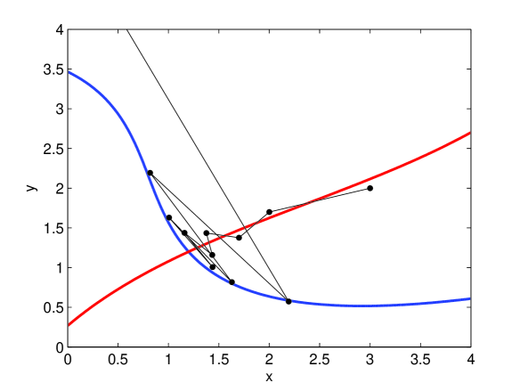
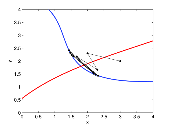
For α=0.2,𝛼0.2\alpha=0.2, β=0,𝛽0\beta=0, which is the case p=0.2𝑝0.2p=0.2 in [13, Section 3.4], we have

U1(x,y)subscript𝑈1𝑥𝑦\displaystyle U_{1}(x,y) =0.4152273992x+0.84913643950.2923863004yabsent0.4152273992𝑥0.84913643950.2923863004𝑦\displaystyle=-0.4152273992x+0.8491364395-0.2923863004y
+0.2419777563(0.4152273992x0.3508635604+0.7076136995y)20.2419777563superscript0.4152273992𝑥0.35086356040.7076136995𝑦2\displaystyle\qquad+0.2419777563(-0.4152273992x-0.3508635604+0.7076136995y)^{2}
0.0974600586(0.4152273992x0.3508635604+0.7076136995y)3,0.0974600586superscript0.4152273992𝑥0.35086356040.7076136995𝑦3\displaystyle\qquad-0.0974600586(-0.4152273992x-0.3508635604+0.7076136995y)^{3},
S1(x,y)subscript𝑆1𝑥𝑦\displaystyle S_{1}(x,y) =0.4152273992x0.3508635604+0.7076136995yabsent0.4152273992𝑥0.35086356040.7076136995𝑦\displaystyle=-0.4152273992x-0.3508635604+0.7076136995y
+0.1961061968(0.4152273992x+0.84913643950.2923863004y)20.1961061968superscript0.4152273992𝑥0.84913643950.2923863004𝑦2\displaystyle\qquad+0.1961061968(-0.4152273992x+0.8491364395-0.2923863004y)^{2}
+0.09806508071(0.4152273992x+0.84913643950.2923863004y)3.0.09806508071superscript0.4152273992𝑥0.84913643950.2923863004𝑦3\displaystyle\qquad+0.09806508071(-0.4152273992x+0.8491364395-0.2923863004y)^{3}.

and

U2(x,y)subscript𝑈2𝑥𝑦\displaystyle U_{2}(x,y) =0.3492151478x+1.2142936330.3253924261yabsent0.3492151478𝑥1.2142936330.3253924261𝑦\displaystyle=-0.3492151478x+1.214293633-0.3253924261y
+0.3059452562(0.3492151478x0.5857063670+0.6746075740y)20.3059452562superscript0.3492151478𝑥0.58570636700.6746075740𝑦2\displaystyle\qquad+0.3059452562(-0.3492151478x-0.5857063670+0.6746075740y)^{2}
0.1066716833(0.3492151478x0.5857063670+0.6746075740y)3,0.1066716833superscript0.3492151478𝑥0.58570636700.6746075740𝑦3\displaystyle\qquad-0.1066716833(-0.3492151478x-0.5857063670+0.6746075740y)^{3},
S2(x,y)subscript𝑆2𝑥𝑦\displaystyle S_{2}(x,y) =0.3492151478x0.5857063670+0.6746075740yabsent0.3492151478𝑥0.58570636700.6746075740𝑦\displaystyle=-0.3492151478x-0.5857063670+0.6746075740y
+0.1446549340(0.3492151478x+1.2142936330.3253924261y)20.1446549340superscript0.3492151478𝑥1.2142936330.3253924261𝑦2\displaystyle\qquad+0.1446549340(-0.3492151478x+1.214293633-0.3253924261y)^{2}
+0.0525187072(0.3492151478x+1.2142936330.3253924261y)3.0.0525187072superscript0.3492151478𝑥1.2142936330.3253924261𝑦3\displaystyle\qquad+0.0525187072(-0.3492151478x+1.214293633-0.3253924261y)^{3}.

Figure 1 shows the graphs of the functions U1(x,y)=0,subscript𝑈1𝑥𝑦0U_{1}(x,y)=0, S1(x,y)=0,subscript𝑆1𝑥𝑦0S_{1}(x,y)=0, U2(x,y)=0subscript𝑈2𝑥𝑦0U_{2}(x,y)=0 and S2(x,y)=0subscript𝑆2𝑥𝑦0S_{2}(x,y)=0 together with a typical trajectory. As it can be seen, the trajectory follows the unstable manifold in both cases.
Refer to caption
(a) Graphs of U1(x,y)=0subscript𝑈1𝑥𝑦0U_{1}(x,y)=0 (blue) and S1(x,y)=0subscript𝑆1𝑥𝑦0S_{1}(x,y)=0 (red) for α=0.2,β=0formulae-sequence𝛼0.2𝛽0\alpha=0.2,\beta=0
Refer to caption
(b) Graphs of U2(x,y)=0subscript𝑈2𝑥𝑦0U_{2}(x,y)=0 (blue) and S2(x,y)=0subscript𝑆2𝑥𝑦0S_{2}(x,y)=0 (red) for α=0.8,β=0formulae-sequence𝛼0.8𝛽0\alpha=0.8,\beta=0
Figure 1: Graphs of stable and unstable manifolds together with a typical trajectory for different values of α𝛼\alpha and β.𝛽\beta.

We would like to note here that the functions U1(x,y),subscript𝑈1𝑥𝑦U_{1}(x,y), S1(x,y),subscript𝑆1𝑥𝑦S_{1}(x,y), U2(x,y)subscript𝑈2𝑥𝑦U_{2}(x,y) and S2(x,y),subscript𝑆2𝑥𝑦S_{2}(x,y), obtained in this example are not the same as those given in [13]. However, they are some certain constant multiples of each other, and hence, the manifolds provided here and given in [13] are the same. So, we recover the results given in [13] by taking β=0.𝛽0\beta=0.

Example 4.2

As another example let us keep α𝛼\alpha the same as in the previous example but change β.𝛽\beta.

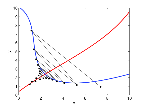
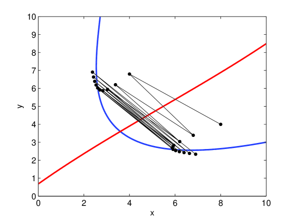
For α=0.2,𝛼0.2\alpha=0.2, β=0.5,𝛽0.5\beta=0.5, we have

U3(x,y)subscript𝑈3𝑥𝑦\displaystyle U_{3}(x,y) =0.4152273992x+0.84913643950.2923863004yabsent0.4152273992𝑥0.84913643950.2923863004𝑦\displaystyle=-0.4152273992x+0.8491364395-0.2923863004y
+0.2419777563(0.4152273992x0.3508635604+0.7076136995y)20.2419777563superscript0.4152273992𝑥0.35086356040.7076136995𝑦2\displaystyle\qquad+0.2419777563(-0.4152273992x-0.3508635604+0.7076136995y)^{2}
0.0974600586(0.4152273992x0.3508635604+0.7076136995y)3,0.0974600586superscript0.4152273992𝑥0.35086356040.7076136995𝑦3\displaystyle\qquad-0.0974600586(-0.4152273992x-0.3508635604+0.7076136995y)^{3},
S3(x,y)subscript𝑆3𝑥𝑦\displaystyle S_{3}(x,y) =0.4152273992x0.3508635604+0.7076136995yabsent0.4152273992𝑥0.35086356040.7076136995𝑦\displaystyle=-0.4152273992x-0.3508635604+0.7076136995y
+0.1961061968(0.4152273992x+0.84913643950.2923863004y)20.1961061968superscript0.4152273992𝑥0.84913643950.2923863004𝑦2\displaystyle\qquad+0.1961061968(-0.4152273992x+0.8491364395-0.2923863004y)^{2}
+0.09806508071(0.4152273992x+0.84913643950.2923863004y)3.0.09806508071superscript0.4152273992𝑥0.84913643950.2923863004𝑦3\displaystyle\qquad+0.09806508071(-0.4152273992x+0.8491364395-0.2923863004y)^{3}.

and

U4(x,y)subscript𝑈4𝑥𝑦\displaystyle U_{4}(x,y) =0.3492151478x+1.2142936330.3253924261yabsent0.3492151478𝑥1.2142936330.3253924261𝑦\displaystyle=-0.3492151478x+1.214293633-0.3253924261y
+0.3059452562(0.3492151478x0.5857063670+0.6746075740y)20.3059452562superscript0.3492151478𝑥0.58570636700.6746075740𝑦2\displaystyle\qquad+0.3059452562(-0.3492151478x-0.5857063670+0.6746075740y)^{2}
0.1066716833(0.3492151478x0.5857063670+0.6746075740y)3,0.1066716833superscript0.3492151478𝑥0.58570636700.6746075740𝑦3\displaystyle\qquad-0.1066716833(-0.3492151478x-0.5857063670+0.6746075740y)^{3},
S4(x,y)subscript𝑆4𝑥𝑦\displaystyle S_{4}(x,y) =0.3492151478x0.5857063670+0.6746075740yabsent0.3492151478𝑥0.58570636700.6746075740𝑦\displaystyle=-0.3492151478x-0.5857063670+0.6746075740y
+0.1446549340(0.3492151478x+1.2142936330.3253924261y)20.1446549340superscript0.3492151478𝑥1.2142936330.3253924261𝑦2\displaystyle\qquad+0.1446549340(-0.3492151478x+1.214293633-0.3253924261y)^{2}
+0.0525187072(0.3492151478x+1.2142936330.3253924261y)3.0.0525187072superscript0.3492151478𝑥1.2142936330.3253924261𝑦3\displaystyle\qquad+0.0525187072(-0.3492151478x+1.214293633-0.3253924261y)^{3}.

Figure 2 shows the graphs of the functions U3(x,y)=0,subscript𝑈3𝑥𝑦0U_{3}(x,y)=0, S3(x,y)=0,subscript𝑆3𝑥𝑦0S_{3}(x,y)=0, U4(x,y)=0subscript𝑈4𝑥𝑦0U_{4}(x,y)=0 and S4(x,y)=0subscript𝑆4𝑥𝑦0S_{4}(x,y)=0 together with a typical trajectory. As it can be seen, the trajectory follows the unstable manifold in both cases.
Refer to caption
(a) Graphs of U3(x,y)=0subscript𝑈3𝑥𝑦0U_{3}(x,y)=0 (blue) and S3(x,y)=0subscript𝑆3𝑥𝑦0S_{3}(x,y)=0 (red) for α=0.2,β=0.5formulae-sequence𝛼0.2𝛽0.5\alpha=0.2,\beta=0.5
Refer to caption
(b) Graphs of U4(x,y)=0subscript𝑈4𝑥𝑦0U_{4}(x,y)=0 (blue) and S4(x,y)=0subscript𝑆4𝑥𝑦0S_{4}(x,y)=0 (red) for α=0.8,β=0.5formulae-sequence𝛼0.8𝛽0.5\alpha=0.8,\beta=0.5
Figure 2: Graphs of stable and unstable manifolds together with a typical trajectory for different values of α𝛼\alpha and β.𝛽\beta.
Example 4.3

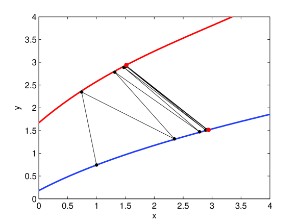
In this example, let us take the parameters as in [13]. Let α=1,𝛼1\alpha=1, β=0.𝛽0\beta=0. Let Φ=2.94.Φ2.94\Phi=2.94. In this case, we have Ψ=1.515463918Ψ1.515463918\Psi=1.515463918 and

C1(x,y;Φ)subscript𝐶1𝑥𝑦Φ\displaystyle C_{1}(x,y;\Phi) =0.1491735785x+0.22606717540.4385703205yabsent0.1491735785𝑥0.22606717540.4385703205𝑦\displaystyle=0.1491735785x+0.2260671754-0.4385703205y
0.08039102209(0.1491735785x1.289396743+0.5614296795y)20.08039102209superscript0.1491735785𝑥1.2893967430.5614296795𝑦2\displaystyle\qquad-0.08039102209(0.1491735785x-1.289396743+0.5614296795y)^{2}
+0.01997063483(0.1491735785x1.289396743+0.5614296795y)30.01997063483superscript0.1491735785𝑥1.2893967430.5614296795𝑦3\displaystyle\qquad+0.01997063483(0.1491735785x-1.289396743+0.5614296795y)^{3}

and

C1(x,y;Ψ)subscript𝐶1𝑥𝑦Ψ\displaystyle C_{1}(x,y;\Psi) =0.5614296798x+1.6506032570.8508264215yabsent0.5614296798𝑥1.6506032570.8508264215𝑦\displaystyle=0.5614296798x+1.650603257-0.8508264215y
0.1559585827(0.5614296798x1.289396743+0.1491735785y)20.1559585827superscript0.5614296798𝑥1.2893967430.1491735785𝑦2\displaystyle\qquad-0.1559585827(0.5614296798x-1.289396743+0.1491735785y)^{2}
+0.05514400545(0.5614296798x1.289396743+0.1491735785y)3.0.05514400545superscript0.5614296798𝑥1.2893967430.1491735785𝑦3\displaystyle\qquad+0.05514400545(0.5614296798x-1.289396743+0.1491735785y)^{3}.

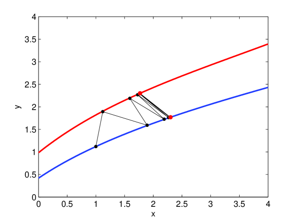
For Φ=2.3,Φ2.3\Phi=2.3, we have Ψ=1.769230769Ψ1.769230769\Psi=1.769230769 and

C2(x,y;Φ)subscript𝐶2𝑥𝑦Φ\displaystyle C_{2}(x,y;\Phi) =0.2506265664x+0.44341623230.5764411027yabsent0.2506265664𝑥0.44341623230.5764411027𝑦\displaystyle=0.2506265664x+0.4434162323-0.5764411027y
0.1137137228(0.2506265664x1.325814536+0.4235588973y)20.1137137228superscript0.2506265664𝑥1.3258145360.4235588973𝑦2\displaystyle\qquad-0.1137137228(0.2506265664x-1.325814536+0.4235588973y)^{2}
+0.03453170706(0.2506265664x1.325814536+0.4235588973y)30.03453170706superscript0.2506265664𝑥1.3258145360.4235588973𝑦3\displaystyle\qquad+0.03453170706(0.2506265664x-1.325814536+0.4235588973y)^{3}

and

C2(x,y;Ψ)subscript𝐶2𝑥𝑦Ψ\displaystyle C_{2}(x,y;\Psi) =0.4235588973x+0.97418546340.7493734336yabsent0.4235588973𝑥0.97418546340.7493734336𝑦\displaystyle=0.4235588973x+0.9741854634-0.7493734336y
0.1478278397(0.4235588973x1.325814536+0.2506265664y)20.1478278397superscript0.4235588973𝑥1.3258145360.2506265664𝑦2\displaystyle\qquad-0.1478278397(0.4235588973x-1.325814536+0.2506265664y)^{2}
+0.0520650698(0.4235588973x1.325814536+0.2506265664y)3.0.0520650698superscript0.4235588973𝑥1.3258145360.2506265664𝑦3\displaystyle\qquad+0.0520650698(0.4235588973x-1.325814536+0.2506265664y)^{3}.

Figure 3 shows the graphs of the functions C1(x,y;Φ)=0,subscript𝐶1𝑥𝑦Φ0C_{1}(x,y;\Phi)=0, C1(x,y;Ψ)=0subscript𝐶1𝑥𝑦Ψ0C_{1}(x,y;\Psi)=0 and C2(x,y;Φ)=0,subscript𝐶2𝑥𝑦Φ0C_{2}(x,y;\Phi)=0, C2(x,y;Ψ)=0,subscript𝐶2𝑥𝑦Ψ0C_{2}(x,y;\Psi)=0, together with typical trajectories. As it can be seen, the trajectory follows the invariant manifold in both cases.
Refer to caption
(a) Graphs of C1(x,y;Φ)=0subscript𝐶1𝑥𝑦Φ0C_{1}(x,y;\Phi)=0 (blue) and C1(x,y;Ψ)=0subscript𝐶1𝑥𝑦Ψ0C_{1}(x,y;\Psi)=0 (red) for Φ=2.94.Φ2.94\Phi=2.94.
Refer to caption
(b) Graphs of C2(x,y;Φ)=0subscript𝐶2𝑥𝑦Φ0C_{2}(x,y;\Phi)=0 (blue) and C2(x,y;Ψ)=0subscript𝐶2𝑥𝑦Ψ0C_{2}(x,y;\Psi)=0 (red) for Φ=2.3.Φ2.3\Phi=2.3.
Figure 3: Graphs of invariant curves together with typical trajectories and periodic solutions for different values of ΦΦ\Phi and β=0.𝛽0\beta=0.
Example 4.4

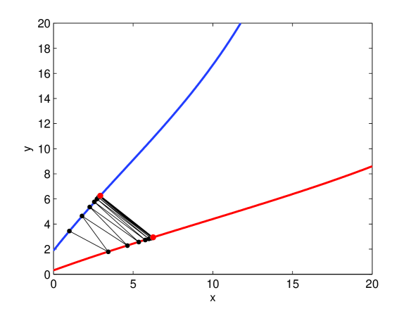
As the last example, let α=1,𝛼1\alpha=1, β=0.5.𝛽0.5\beta=0.5. For Φ=2.94,Φ2.94\Phi=2.94, we have Ψ=6.255319149Ψ6.255319149\Psi=6.255319149 and

C3(x,y;Φ)subscript𝐶3𝑥𝑦Φ\displaystyle C_{3}(x,y;\Phi) =1.071618354x+1.6239989470.7632795057yabsent1.071618354𝑥1.6239989470.7632795057𝑦\displaystyle=1.071618354x+1.623998947-0.7632795057y
0.006468848599(1.071618354x4.631320202+0.2367204943y)20.006468848599superscript1.071618354𝑥4.6313202020.2367204943𝑦2\displaystyle\qquad-0.006468848599(1.071618354x-4.631320202+0.2367204943y)^{2}
+0.001026052614(1.071618354x4.631320202+0.2367204943y)30.001026052614superscript1.071618354𝑥4.6313202020.2367204943𝑦3\displaystyle\qquad+0.001026052614(1.071618354x-4.631320202+0.2367204943y)^{3}

and

C3(x,y;Ψ)subscript𝐶3𝑥𝑦Ψ\displaystyle C_{3}(x,y;\Psi) =0.1416540319x+0.16860844270.3587413677yabsent0.1416540319𝑥0.16860844270.3587413677𝑦\displaystyle=0.1416540319x+0.1686084427-0.3587413677y
0.005080796064(0.1416540319x2.771391557+0.6412586323y)20.005080796064superscript0.1416540319𝑥2.7713915570.6412586323𝑦2\displaystyle\qquad-0.005080796064(0.1416540319x-2.771391557+0.6412586323y)^{2}
+0.001395071806(0.1416540319x2.771391557+0.6412586323y)3.0.001395071806superscript0.1416540319𝑥2.7713915570.6412586323𝑦3\displaystyle\qquad+0.001395071806(0.1416540319x-2.771391557+0.6412586323y)^{3}.

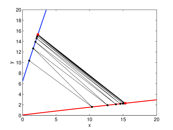
For Φ=2.3,Φ2.3\Phi=2.3, we have Ψ=15.33333333Ψ15.33333333\Psi=15.33333333 and

C4(x,y;Φ)subscript𝐶4𝑥𝑦Φ\displaystyle C_{4}(x,y;\Phi) =3.473613893x+6.1456245860.9218436874yabsent3.473613893𝑥6.1456245860.9218436874𝑦\displaystyle=3.473613893x+6.145624586-0.9218436874y
0.001973405924(3.473613893x9.187708748+0.07815631264y)20.001973405924superscript3.473613893𝑥9.1877087480.07815631264𝑦2\displaystyle\qquad-0.001973405924(3.473613893x-9.187708748+0.07815631264y)^{2}
+0.000140325572(3.473613893x9.187708748+0.07815631264y)30.000140325572superscript3.473613893𝑥9.1877087480.07815631264𝑦3\displaystyle\qquad+0.000140325572(3.473613893x-9.187708748+0.07815631264y)^{3}

and

C4(x,y;Ψ)subscript𝐶4𝑥𝑦Ψ\displaystyle C_{4}(x,y;\Psi) =0.01938877756x+0.02074148290.1382765531yabsent0.01938877756𝑥0.02074148290.1382765531𝑦\displaystyle=0.01938877756x+0.0207414829-0.1382765531y
0.001193222187(0.01938877756x2.279258517+0.8617234469y)20.001193222187superscript0.01938877756𝑥2.2792585170.8617234469𝑦2\displaystyle\qquad-0.001193222187(0.01938877756x-2.279258517+0.8617234469y)^{2}
+0.0003847285557(0.01938877756x2.279258517+0.8617234469y)3.0.0003847285557superscript0.01938877756𝑥2.2792585170.8617234469𝑦3\displaystyle\qquad+0.0003847285557(0.01938877756x-2.279258517+0.8617234469y)^{3}.

Figure 4 shows the graphs of the functions C3(x,y;Φ)=0,subscript𝐶3𝑥𝑦Φ0C_{3}(x,y;\Phi)=0, C3(x,y;Ψ)=0subscript𝐶3𝑥𝑦Ψ0C_{3}(x,y;\Psi)=0 and C4(x,y;Φ)=0,subscript𝐶4𝑥𝑦Φ0C_{4}(x,y;\Phi)=0, C4(x,y;Ψ)=0,subscript𝐶4𝑥𝑦Ψ0C_{4}(x,y;\Psi)=0, together with typical trajectories. As it can be seen, the trajectory follows the invariant manifold in both cases.
Refer to caption
(a) Graphs of C3(x,y;Φ)=0subscript𝐶3𝑥𝑦Φ0C_{3}(x,y;\Phi)=0 (blue) and C3(x,y;Ψ)=0subscript𝐶3𝑥𝑦Ψ0C_{3}(x,y;\Psi)=0 (red) for Φ=2.94.Φ2.94\Phi=2.94.
Refer to caption
(b) Graphs of C4(x,y;Φ)=0subscript𝐶4𝑥𝑦Φ0C_{4}(x,y;\Phi)=0 (blue) and C4(x,y;Ψ)=0subscript𝐶4𝑥𝑦Ψ0C_{4}(x,y;\Psi)=0 (red) for Φ=2.3.Φ2.3\Phi=2.3.
Figure 4: Graphs of invariant curves together with typical trajectories and periodic solutions for different values of ΦΦ\Phi and β=0.5.𝛽0.5\beta=0.5.

References

  • [1] Agarwal RP. Difference Equations and Inequalities: Theory, Methods, And Applications. Marcel Dekker Inc, New York, 2000.
  • [2] Aksoy A, Turan M. On the dynamics of the non-linear difference equation xn+1=α+βxn1+xn1/xn.subscript𝑥𝑛1𝛼𝛽subscript𝑥𝑛1subscript𝑥𝑛1subscript𝑥𝑛x_{n+1}=\alpha+\beta x_{n-1}+x_{n-1}/x_{n}. Science Asia; 2015; 41(5); 350–356.
  • [3] Amleh AM, Grove EA, Ladas G, Georgiou DA. On the recursive sequence xn+1=α+xn1/xn.subscript𝑥𝑛1𝛼subscript𝑥𝑛1subscript𝑥𝑛x_{n+1}=\alpha+x_{n-1}/x_{n}. J. Math. Anal. Appl.; 1999; 233; 790–798.
  • [4] Burgić Dž, Kalabušić S, Kulenović MRS. Non-hyperbolic dynamics for competitive systems in the plane and global period-doubling bifurcations. Adv. Dyn. Syst. Appl.; 2008; 3; 229–249.
  • [5] Carr J. Applications of center manifold theory. Springer-Verlag, New York, 1981.
  • [6] Elaydi S. An Introduction to Difference Equations. Springer-Verlag, New York, 1999.
  • [7] Hale JK, Koçak H. Dynamics and Bifurcations, Texts in Applied Mathematics 3. Springer-Verlag, New York, 1991.
  • [8] Hamza AE. On the difference equation xn+1=α+xn1/xn.subscript𝑥𝑛1𝛼subscript𝑥𝑛1subscript𝑥𝑛x_{n+1}=\alpha+x_{n-1}/x_{n}. J. Math. Anal. Appl.; 2006; 322; 668–674.
  • [9] Kelley WG, Peterson AC. Difference equations: an introduction with applications. Academic Press, New York, 2001.
  • [10] Kocic VL, Ladas G. Global Behavior of Nonlinear Difference Equations of Higher Order with Applications. Kluwer Academic Publishers, Dordrecht, 1993.
  • [11] Kulenović MRS, Ladas G. Dynamics of second order rational difference equations with open problems and conjectures. Chapman & Hall/CRC, New York, 2002.
  • [12] Kulenović MRS, Merino O. Discrete Dynamical Systems and Difference Equations with Mathematica. Chapman and Hall/CRC, Boca Raton, London, 2002.
  • [13] Kulenović MRS and Pilav E. Asymptotic approximations of the stable and unstable manifold of the fixed point of a certain rational map by using functional equations. Sarajevo Journal of Mathematics; 2016; 12 (25); 233–250.
  • [14] Lakshmikantham V, Trigiante D. Theory of difference equations: numerical methods and applications. Marcel Dekker, New York, 2002.
  • [15] Marsden J, McCracken M. The Hopf Bifurcation and Its Application. Springer-Verlag, New York, 1976.
  • [16] Sedaghat H. Nonlinear Difference Equations: Theory with Applications to Social Science Models. Kluwer Academic, USA, 2003.
  • [17] Stević S. On the difference equation xn+1=α+xn1xn.subscript𝑥𝑛1𝛼subscript𝑥𝑛1subscript𝑥𝑛x_{n+1}=\alpha+\frac{x_{n-1}}{x_{n}}. Computers and Mathematics with Applications; 2008; 56; 1159–1171.
  • [18] Wiggins S. Introduction to Applied Nonlinear Dynamical Systems and Chaos, Second edition. Texts in Applied Mathematics, 2. Springer-Verlag, New York, 2003.