Wideband Super-resolution Imaging in Radio Interferometry via Low Rankness and Joint Average Sparsity Models (HyperSARA)

Abdullah Abdulaziz, Arwa Dabbech and Yves Wiaux
Institute of Sensors, Signals and Systems, Heriot-Watt University, Edinburgh EH14 4AS, UK
E-mail: aa61@hw.ac.uk
(Accepted XXX. Received YYY; in original form ZZZ)
Abstract

We propose a new approach within the versatile framework of convex optimization to solve the radio-interferometric wideband imaging problem. Our approach, dubbed HyperSARA, leverages low rankness and joint average sparsity priors to enable formation of high resolution and high dynamic range image cubes from visibility data. The resulting minimization problem is solved using a Primal-Dual (PD) algorithm. The algorithmic structure is shipped with highly interesting functionalities such as preconditioning for accelerated convergence, and parallelization enabling to spread the computational cost and memory requirements across a multitude of processing nodes with limited resources. In this work, we provide a proof of concept for wideband image reconstruction of megabyte-size images. The better performance of HyperSARA, in terms of resolution and dynamic range of the formed images, compared to single channel imaging and the clean-based wideband imaging algorithm in the wsclean software, is showcased on simulations and real VLA observations. Our matlab code is available online on github.

keywords:
techniques: image processing – techniques: interferometric.
pubyear: 2017pagerange: Wideband Super-resolution Imaging in Radio Interferometry via Low Rankness and Joint Average Sparsity Models (HyperSARA)A

1 Introduction

The new generation radio interferometers, such as the Square Kilometre Array (SKA) (Dewdney et al., 2013), the LOw Frequency ARray (LOFAR) (Van Haarlem et al., 2013) and the recently upgraded Karl G. Jansky Very Large Array (VLA) (Perley et al., 2011), will probe new regimes of radio emissions, thanks to their extreme resolution and sensitivity, wide bandwidth and ability to map large areas of the radio sky. These instruments will deepen our knowledge in cosmology and astrophysics. SKA in particular is expected to achieve fundamental science goals such as probing the Epoch of Re-ionization (EoR) (Koopmans et al., 2015) and investigating cosmic magnetism (Melanie et al., 2014). It will provide maps with sub-arcsec resolution over thousands of frequency channels, and is expected to produce giga pixel sized images with up to seven orders of magnitude dynamic range (Dewdney et al., 2013). Handling the huge amounts of data (\approx terabytes) is a tremendous challenge for the coming years. To meet the capabilities of such powerful instruments, hence deliver the expected science goals, novel imaging techniques that are both robust and scalable are needed.

In the context of wideband imaging, the aim is to jointly recover the spatial and spectral information of the radio emission. A straightforward approach is to image each channel separately, i.e. no inter-channel information is exploited. Although, single channel image recovery has been extensively studied in the literature (e.g. Högbom, 1974; Schwab & Cotton, 1983; Bhatnagar & Cornwell, 2004; Cornwell, 2008; Wiaux et al., 2009; Li, F. et al., 2011; Dabbech et al., 2012; Carrillo et al., 2012, 2014; Offringa et al., 2014; Garsden et al., 2015; Dabbech et al., 2015; Girard et al., 2015; Junklewitz et al., 2016; Onose et al., 2016b; Onose et al., 2017; Pratley et al., 2017; Dabbech et al., 2018), it remains sub-optimal for wideband imaging since the correlation of the wideband data is not exploited. Moreover, the quality of the recovered wideband images is limited to their inherent resolution and sensitivity.
Several approaches have been devised in the literature for the joint recovery of the wideband radio-interferometric (RI) image cube. The first class of methods rely on the clean framework (Högbom, 1974; Clark, 1980; Schwab & Cotton, 1983). clean is a greedy deconvolution method based on iterative local removal of the Point Spread Function (PSF). It can also be seen as a gradient descent approach with implicit sparsity of the sky in the image domain (Onose et al., 2016b). A first clean-based approach, dubbed MF-CLEAN (Sault & Wieringa, 1994), models the sky intensity as a collection of point sources whose spectra follow a power law defined as 𝒙l=𝒙0(νlν0)𝜶subscript𝒙𝑙subscript𝒙0superscriptsubscript𝜈𝑙subscript𝜈0𝜶\boldsymbol{x}_{l}=\boldsymbol{x}_{0}~{}(\frac{\nu_{l}}{\nu_{0}})^{-\boldsymbol{\alpha}}, where 𝒙lsubscript𝒙𝑙\boldsymbol{x}_{l} is the sky image at the frequency νlsubscript𝜈𝑙\nu_{l} and 𝜶𝜶\boldsymbol{\alpha} is the spectral index map. This power law is approximated by a first order (linear) Taylor expansion. The Taylor coefficient images are computed via a least squares solution and the spectral index map is derived from the coefficient images. Yet, MF-CLEAN is sub-optimal when it comes to the recovery of wideband extended emissions, as these are modeled with point sources. Rau & Cornwell (2011) have proposed a multi-scale multi-frequency variant of clean, dubbed MS-MFS, assuming the curvature model as a spectral model. It reads 𝒙l=𝒙0(νlν0)𝜶+𝜷log(νlν0),subscript𝒙𝑙subscript𝒙0superscriptsubscript𝜈𝑙subscript𝜈0𝜶𝜷subscript𝜈𝑙subscript𝜈0\boldsymbol{x}_{l}=\boldsymbol{x}_{0}~{}(\frac{\nu_{l}}{\nu_{0}})^{-\boldsymbol{\alpha}+\boldsymbol{\beta}\log(\frac{\nu_{l}}{\nu_{0}})}, where 𝜶𝜶\boldsymbol{\alpha} and 𝜷𝜷\boldsymbol{\beta} are the spectral index and the curvature maps, respectively. Using Taylor series, 𝒙lsubscript𝒙𝑙\boldsymbol{x}_{l} is approximated via a linear combination of few Taylor coefficient images {𝒔t}t𝒞Tsubscriptsubscript𝒔𝑡for-all𝑡subscript𝒞𝑇\{\boldsymbol{s}_{t}\}_{\forall t\in\mathcal{C}_{T}}111We define a set 𝒞jsubscript𝒞𝑗\mathcal{C}_{j} as: 𝒞j={1,,j}subscript𝒞𝑗1𝑗\mathcal{C}_{j}=\{1,\cdots,j\}., i.e. 𝒙l=t=1Thlt𝒔tsubscript𝒙𝑙superscriptsubscript𝑡1𝑇subscript𝑙𝑡subscript𝒔𝑡\boldsymbol{x}_{l}=\sum_{t=1}^{T}h_{lt}\boldsymbol{s}_{t}, where {hlt=(νlν0ν0)t}(l,t)𝒞L×𝒞Tsubscriptsubscript𝑙𝑡superscriptsubscript𝜈𝑙subscript𝜈0subscript𝜈0𝑡for-all𝑙𝑡subscript𝒞𝐿subscript𝒞𝑇\{h_{lt}={(\frac{\nu_{l}-\nu_{0}}{\nu_{0}})}^{t}\}_{\forall(l,t)\in\mathcal{C}_{L}\times\mathcal{C}_{T}} are the spectral basis functions, T𝑇T is the order of Taylor series and L𝐿L is the number of channels. In this case, the wideband image reconstruction problem reduces to the recovery of the Taylor coefficient images. These are deconvolved by performing a classical multi-scale clean on their associated dirty images {𝒔tdirty=l=1Lhlt𝒙ldirty}t𝒞Tsubscriptsuperscriptsubscript𝒔𝑡𝑑𝑖𝑟𝑡𝑦superscriptsubscript𝑙1𝐿subscript𝑙𝑡superscriptsubscript𝒙𝑙𝑑𝑖𝑟𝑡𝑦for-all𝑡subscript𝒞𝑇\{\boldsymbol{s}_{t}^{dirty}=\sum_{l=1}^{L}h_{lt}\boldsymbol{x}_{l}^{dirty}\}_{\forall t\in\mathcal{C}_{T}}. More recently, Offringa & Smirnov (2017) have proposed a wideband variant of multi-scale clean, so-called Joined Channel clean (JC-CLEAN), that is incorporated in the software wsclean222W-Stacking clean (wsclean) is a wide field RI imaging software can be found at https://sourceforge.net/projects/wsclean/. (Offringa et al., 2014). The main idea consists in determining the pixel positions of the clean components from an integrated image, obtained as a sum of the residual images of all the channels (initially, these correspond to the dirty images). The spectra of the selected pixel positions are determined directly from the associated values in the residual images at the different channels. When the spectral behaviour of the radio sources is known to be smooth (that is the case for synchrotron emission (Rybicki & Lightman, 2008)), a polynomial is fitted to their estimated spectra.

The second class of methods consists in Bayesian inference techniques. Junklewitz et al. (2015) have considered a power law spectral model. In this case, the reconstruction of the wideband model cube consists in the estimation of the sky image at the reference frequency and the spectral index map. However, the method is limited by higher order spectral effects like spectral curvature.

The third class of approaches define the wideband RI imaging problem as an optimization task involving spatio-spectral regularizations. Wenger & Magnor (2014) have assumed that the spectra are composed of a smooth continuous part with sparse local deviations, hence allowing for recovering non-smooth spectra. The authors have proposed a convex unconstrained minimization problem promoting sparsity-by-synthesis in a concatenation of two dictionaries. The first synthesis dictionary consists of delta functions. Sparsity of its associated synthesis coefficients is enforced, allowing for sparse local deviations. The second synthesis dictionary consists of smooth polynomials, more precisely, the basis functions of Chebyshev polynomials. Joint sparsity of the synthesis coefficients associated with the overall dictionary is also enforced. Assuming smooth spectra, Ferrari et al. (2015) have proposed a convex unconstrained minimization problem promoting sparsity-by-analysis of both the spatial and spectral information. Spatial sparsity is promoted in a redundant wavelet dictionary. More interestingly, sparsity of the spectra is enforced in a Discrete Cosine Transform (DCT). Finally, a third quadratic regularization promoting smoothness of the overall model cube is adopted. The approach involves the tuning of multiple hyper-parameters, representing the trade-off between the different priors. The choice of these parameters is crucial as it affects significantly the final solution. To alleviate the issue of tuning multiple parameters, Deguignet et al. (2016) have discarded the smooth prior on the model cube, reducing the number of hyper-parameters to two. Furthermore, Ammanouil et al. (2017) have proposed an automatic procedure to tune the remaining two hyper-parameters. Abdulaziz et al. (2016) have adopted the linear mixture model, which assumes that the sky intensity images at the different frequencies {𝒙l}l𝒞Lsubscriptsubscript𝒙𝑙for-all𝑙subscript𝒞𝐿\{\boldsymbol{x}_{l}\}_{\forall l\in\mathcal{C}_{L}} can be interpreted as a linear combination of few sources {𝒔q}q𝒞Qsubscriptsubscript𝒔𝑞for-all𝑞subscript𝒞𝑄\{\boldsymbol{s}_{q}\}_{\forall q\in\mathcal{C}_{Q}} each of them has a distinct spectral signature 𝒉qsubscript𝒉𝑞\boldsymbol{h}_{q}, i.e. {𝒙l=q=1Qhlq𝒔q}l𝒞Lsubscriptsubscript𝒙𝑙superscriptsubscript𝑞1𝑄subscript𝑙𝑞subscript𝒔𝑞for-all𝑙subscript𝒞𝐿\{\boldsymbol{x}_{l}=\sum_{q=1}^{Q}h_{lq}\boldsymbol{s}_{q}\}_{\forall l\in\mathcal{C}_{L}}, where Q𝑄Q is the number of sources and L𝐿L is the number of channels. Authors have presented a convex constrained minimization problem promoting low rankness and joint average sparsity of the wideband model cube. The authors have also shown that the combination of these two priors is highly efficient in capturing the correlation across the channels. Jiang et al. (2017) have also adopted the linear mixture model and have proposed a projected least squares algorithm built upon a sparse signal model to reconstruct explicitly the sources and their spectra. The recovery of the wideband image cube is reduced to the estimation of two thin matrices. This decreases the computational cost and the memory requirements of the algorithm. However, the problem is non-convex and therefore could have local optimums. Moreover, the number of sources has to be specified in advance.

The work herein fits within the last class of methods and extends our recent works in Abdulaziz et al. (2016, 2017). Our proposed approach, dubbed HyperSARA, solves a sequence of weighted nuclear norm and 2,1subscript21\ell_{2,1} minimization problems, aiming to approximate low rankness and joint average sparsity in 0subscript0\ell_{0} sense. An adaptive Preconditioned Primal-Dual (PPD) algorithm is adopted to solve the minimization problem. The algorithmic structure involves an adaptive strategy to estimate the noise level with respect to calibration errors present in real data (Dabbech et al., 2018). We study the reconstruction performance of our approach on simulations and real VLA observations in comparison with the single channel imaging (Onose et al., 2017; Dabbech et al., 2018) and the wideband deconvolution algorithm JC-CLEAN (Offringa & Smirnov, 2017).

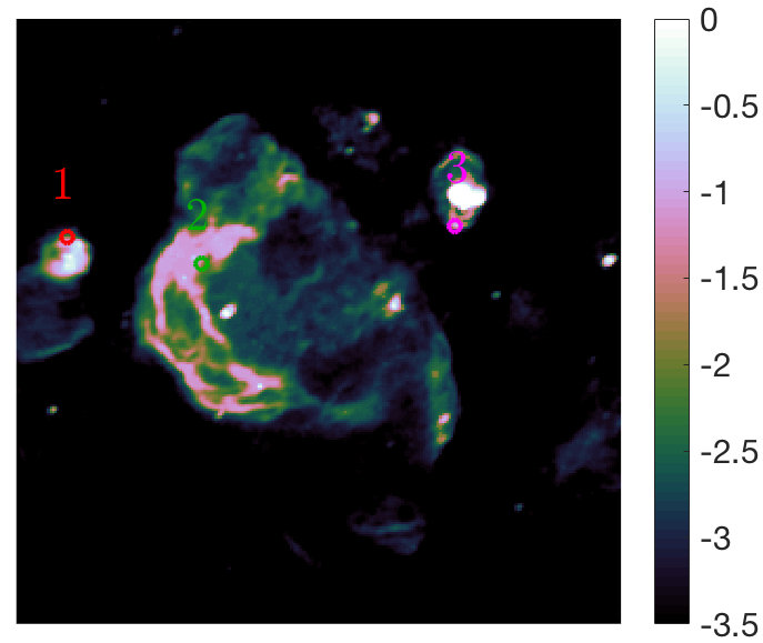
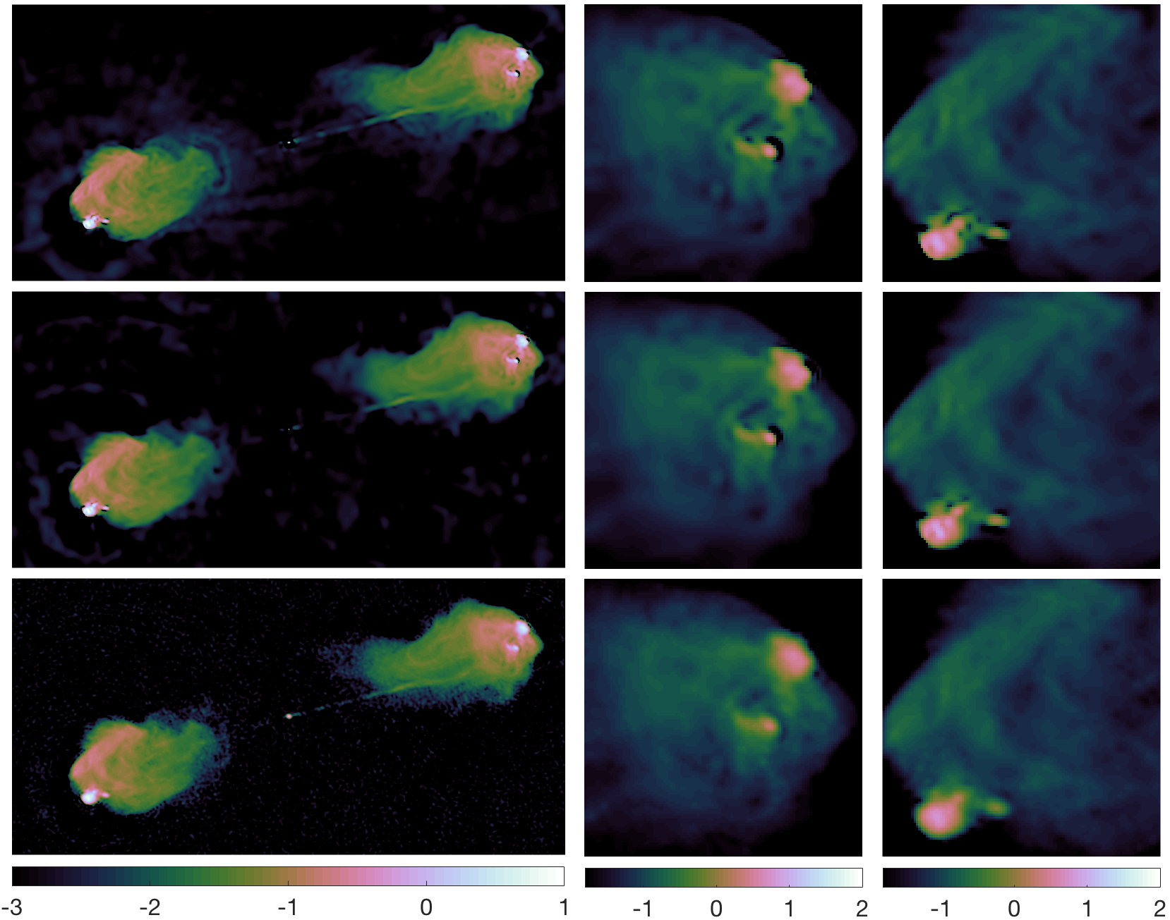
The remainder of the article is structured as follows. In Section 2, we recall the wideband RI imaging problem and explain the low rankness and joint sparsity priors on the wideband model cube. We also present the HyperSARA minimization task. In Section 3, we provide intuitive and complete descriptions of the HyperSARA algorithmic structure. Analysis of the proposed approach and comparison with the benchmark methods on simulations are given in Section 4. Imaging results of VLA observations of Cyg A and the supernova remnant G055.7+3.4 are presented in Section 5. Finally, conclusions are stated in Section 6.

2 HyperSARA: optimization problem

In this section, we recall the wideband RI measurement model. We also revisit the low rankness and joint sparsity model adopted here for wideband RI imaging. We finally present the HyperSARA minimization problem.

2.1 Wideband RI data model

A radio interferometer is an array of spatially separated antennas probing the radio waves emanating from astrophysical sources. Each antenna pair gives access to a radio measurement, dubbed visibility, corresponding to the cross-correlation of the sensed electric field Eνsubscript𝐸𝜈E_{\nu} at a frequency ν𝜈\nu. We define a baseline 𝒃ij3subscript𝒃𝑖𝑗superscript3\boldsymbol{b}_{ij}\in\mathbb{R}^{3} as the vectorial distance between two antennas i𝑖i and j𝑗j, and its components (u¯,υ¯,w¯)¯𝑢¯𝜐¯𝑤(\bar{u},\bar{\upsilon},\bar{w}) are in units of meter; w¯¯𝑤\bar{w} denotes the component in the direction of line of sight and 𝒖¯=(u¯,υ¯)bold-¯𝒖¯𝑢¯𝜐\boldsymbol{\bar{u}}=(\bar{u},\bar{\upsilon}) are the coordinates in its perpendicular plane. Assuming non-polarized signal, at each frequency ν𝜈\nu, the visibilities are related to the sky brightness distribution I𝐼I as follows:

y(𝒖¯,w¯,ν)=n(𝒍)1A(𝒍,ν)e2iπνcw¯(n(𝒍)1)I(𝒍,ν)e2iπνc𝒖¯𝒍d2𝒍,𝑦bold-¯𝒖¯𝑤𝜈𝑛superscript𝒍1𝐴𝒍𝜈superscript𝑒2𝑖𝜋𝜈𝑐¯𝑤𝑛𝒍1𝐼𝒍𝜈superscript𝑒2𝑖𝜋𝜈𝑐bold-¯𝒖𝒍superscriptd2𝒍y(\boldsymbol{\bar{u}},\bar{w},\nu)=\int n(\boldsymbol{l})^{-1}A(\boldsymbol{l},\nu)e^{-2i\pi\frac{\nu}{c}\bar{w}(n(\boldsymbol{l})-1)}I(\boldsymbol{l},\nu)e^{-2i\pi\frac{\nu}{c}\boldsymbol{\bar{u}}\cdot\boldsymbol{l}}\textrm{d}^{2}\boldsymbol{l}, (1)

where 𝒍=(l,m)𝒍𝑙𝑚\boldsymbol{l}=(l,m) are the coordinates of a point source in the sky in a parallel plane to the (u¯,υ¯)¯𝑢¯𝜐(\bar{u},\bar{\upsilon}) plane and n=1l2m2𝑛1superscript𝑙2superscript𝑚2n=\sqrt{1-l^{2}-m^{2}} is the coordinate on the line of sight (Thompson et al., 2007). A(𝒍,ν)𝐴𝒍𝜈A(\boldsymbol{l},\nu) denotes the primary beam of the telescope and c𝑐c is the speed of light. Typically, the image reconstruction is performed directly for x(𝒍,ν)=n(𝒍)1A(𝒍,ν)I(𝒍,ν)𝑥𝒍𝜈𝑛superscript𝒍1𝐴𝒍𝜈𝐼𝒍𝜈x(\boldsymbol{l},\nu)=~{}n(\boldsymbol{l})^{-1}~{}A(\boldsymbol{l},\nu)~{}I(\boldsymbol{l},\nu). In theory, the sky intensity I𝐼I can be extracted by a simple division by the primary beam, if all the antennas are identical. This does not always hold in practice and the primary beam constitutes a Direction Dependent Effect (DDE) that requires calibration. More generally, the sky intensity image is modulated with multiple DDEs which encompass instrumental discrepancies, phase distortions induced by the propagation medium, and receivers errors. These effects necessitate calibration which is not in the scope of this article. When the array is coplanar with respect to the direction of observation (w¯=0¯𝑤0\bar{w}=0) or the field of view is narrow (n1𝑛1n\thickapprox 1), and if we consider the sky intensity map to be already multiplied by the primary beam, the complex visibilities y(:,:,ν)𝑦::𝜈y(:,:,\nu) at a frequency ν𝜈\nu reduce to Fourier components of the original sky x(:,ν)𝑥:𝜈x(:,\nu) according to the Van Cittert Zernike theorem (Thompson et al., 2007). Due to the finite number of antennas, the Fourier components are measured at specific spatial frequencies νc(u¯,υ¯)𝜈𝑐¯𝑢¯𝜐\frac{\nu}{c}(\bar{u},\bar{\upsilon}) identifying the so-called uυ𝑢𝜐u\upsilon-coverage of the radio interferometer. In this setting, the Fourier sampling is such that high Fourier modes are probed at higher frequency channels and low Fourier modes are probed at low frequency channels.

Considering L𝐿L channels and sketching the intensity images and the RI data at each frequency νlsubscript𝜈𝑙\nu_{l} as vectors, the discrete version of the measurement model follows:

𝒚l=𝚽l𝒙l+𝒘lwith𝚽l=𝚯l𝗚l𝗙𝗭,formulae-sequencesubscript𝒚𝑙subscript𝚽𝑙subscript𝒙𝑙subscript𝒘𝑙withsubscript𝚽𝑙subscript𝚯𝑙subscript𝗚𝑙𝗙𝗭{\boldsymbol{y}}_{l}=\boldsymbol{\Phi}_{l}{\boldsymbol{x}}_{l}+{\boldsymbol{w}}_{l}\quad\text{with}\quad\boldsymbol{\Phi}_{l}={\boldsymbol{\Theta}}_{l}{\boldsymbol{\mathsf{G}}}_{l}\boldsymbol{\mathsf{F}}\boldsymbol{\mathsf{Z}}, (2)

where 𝒙l+Nsubscript𝒙𝑙subscriptsuperscript𝑁{\boldsymbol{x}}_{l}\in\mathbb{R}^{N}_{+} is the unknown intensity image, and 𝒚lMsubscript𝒚𝑙superscript𝑀{\boldsymbol{y}}_{l}\in\mathbb{C}^{M} represents the complex Fourier measurements corrupted with additive white Gaussian noise 𝒘lMsubscript𝒘𝑙superscript𝑀{\boldsymbol{w}}_{l}\in\mathbb{C}^{M}. 𝚽lsubscript𝚽𝑙\boldsymbol{\Phi}_{l} is the sensing matrix at the frequency νlsubscript𝜈𝑙\nu_{l}, modeling the non-uniform sampling of the measurements in the Fourier domain. The de-gridding matrix 𝗚lM×oNsubscript𝗚𝑙superscript𝑀𝑜𝑁{\boldsymbol{\mathsf{G}}}_{l}\in\mathbb{C}^{M\times o\cdot N} has a convolution kernel on its rows to interpolate the continuous visibilities from a regular grid. 𝗙oN×oN𝗙superscript𝑜𝑁𝑜𝑁{\boldsymbol{\mathsf{F}}}\in\mathbb{C}^{o\cdot N\times o\cdot N} is the Fast Fourier Transform (FFT) matrix. 𝗭oN×N𝗭superscript𝑜𝑁𝑁{\boldsymbol{\mathsf{Z}}}\in\mathbb{R}^{o\cdot N\times N} accounts for the oversampling and corrects for possible imperfections in the interpolation. The matrix 𝚯lM×Msubscript𝚯𝑙superscript𝑀𝑀{\boldsymbol{\Theta}}_{l}\in\mathbb{C}^{M\times M} is the weighting matrix containing on the diagonal the natural weights, i.e. the inverse of the noise standard deviation. Note that the data 𝒚lsubscript𝒚𝑙\boldsymbol{y}_{l} are the naturally-weighted RI measurements, i.e. 𝒚l=𝚯l𝒚¯lsubscript𝒚𝑙subscript𝚯𝑙subscript¯𝒚𝑙\boldsymbol{y}_{l}={\boldsymbol{\Theta}}_{l}\bar{\boldsymbol{y}}_{l}, where 𝒚¯lMsubscript¯𝒚𝑙superscript𝑀\bar{\boldsymbol{y}}_{l}\in\mathbb{C}^{M} are the RI measurements.

The wideband RI data cube is written in a matrix form as 𝗬=(𝒚1,..,𝒚L)M×L\boldsymbol{\mathsf{Y}}=({\boldsymbol{y}}_{1},..,{\boldsymbol{y}}_{L})\in\mathbb{C}^{M\times L}, so are the wideband RI model cube 𝗫=(𝒙1,..,𝒙L)+N×L{\boldsymbol{\mathsf{X}}}=({\boldsymbol{x}}_{1},..,{\boldsymbol{x}}_{L})\in\mathbb{R}_{+}^{N\times L} and the additive white Gaussian noise 𝗪=(𝒘1,..,𝒘L)M×L{\boldsymbol{\mathsf{W}}}=({\boldsymbol{w}}_{1},..,{\boldsymbol{w}}_{L})\in\mathbb{C}^{M\times L}. The wideband linear operator ΦΦ\Phi is defined such that Φ(𝗫)=([𝚽l𝒙l]l𝒞L)Φ𝗫subscriptdelimited-[]subscript𝚽𝑙subscript𝒙𝑙for-all𝑙subscript𝒞𝐿{\Phi(\boldsymbol{\mathsf{X}})}=([\boldsymbol{\Phi}_{l}{\boldsymbol{x}}_{l}]_{\forall l\in\mathcal{C}_{L}}). Following these notations, the wideband RI data model reads:

𝗬=Φ(𝗫)+𝗪.𝗬Φ𝗫𝗪\boldsymbol{\mathsf{Y}}=\Phi(\boldsymbol{\mathsf{X}})+\boldsymbol{\mathsf{W}}. (3)

The problem of recovering the wideband sky 𝗫𝗫\boldsymbol{\mathsf{X}} from the incomplete and noisy RI data 𝗬𝗬\boldsymbol{\mathsf{Y}} is an ill-posed inverse problem. Thus, enforcing only data fidelity is insufficient and a prior knowledge on the unknown wideband sky is needed to get an accurate approximation. The quality of reconstruction is highly dependent on the choice of the wideband sky model.

2.2 Low rankness and joint sparsity sky model

In the context of wideband RI image reconstruction, we adopt the linear mixture model originally proposed by (Golbabaee & Vandergheynst, 2012). It assumes that the wideband sky is a linear combination of few sources, each having a distinct spectral signature (Abdulaziz et al., 2016, 2017). Following this model, the wideband model cube reads:

𝗫=𝗦𝗛,𝗫superscript𝗦𝗛\boldsymbol{\mathsf{X}}=\boldsymbol{\mathsf{S}}\boldsymbol{\mathsf{H}}^{\dagger}, (4)

where the matrix 𝗦=(𝒔1,..,𝒔Q)N×Q{\boldsymbol{\mathsf{S}}}=({\boldsymbol{s}}_{1},..,{\boldsymbol{s}}_{Q})\in\mathbb{R}^{N\times Q} represents the physical sources present in the sky, and their corresponding spectral signatures constitute the columns of the mixing matrix 𝗛=(𝒉1,..,𝒉Q)L×Q\boldsymbol{\mathsf{H}}=({\boldsymbol{h}}_{1},..,{\boldsymbol{h}}_{Q})\in\mathbb{R}^{L\times Q}. Note that, in this model, physical sources with similar spectral behaviour will be considered as one “source”defining one column of the matrix 𝗦𝗦\boldsymbol{\mathsf{S}}. Recall that solving for 𝗦𝗦\boldsymbol{\mathsf{S}} and 𝗛𝗛\boldsymbol{\mathsf{H}} would explicitly imply a source separation problem, that is a non-linear non-convex problem. Instead, we leverage convex optimization by solving directly for 𝗫𝗫\boldsymbol{\mathsf{X}} with appropriate priors. The linear mixture model implies low rankness of 𝗫𝗫\boldsymbol{\mathsf{X}}, as the rank is upper bounded by the number of “sources”. It also implies joint sparsity over the spectral channels; when all the sources are inactive at one pixel position and regardless of their spectral indices, a full row of the matrix 𝗫𝗫\boldsymbol{\mathsf{X}} will be automatically equal to zero.

Given the nature of the RI Fourier sampling where the uυ𝑢𝜐u\upsilon-coverage dilates with respect to frequency, the combination of low rankness and joint sparsity results in higher resolution and higher dynamic range of the reconstructed RI model cube. On the one hand, enforcing low rankness implies correlation across the channels, this enhances the recovery of extended emissions at the high frequency channels and captures the high spatial frequency content at the low frequency channels. On the other hand, promoting joint sparsity results in the rejection of isolated pixels that are associated to uncorrelated noise since low energy rows of 𝗫𝗫\boldsymbol{\mathsf{X}} are fully set to zero. Consequently, the overall dynamic range of the reconstructed cube is increased.

The linear mixture model is similar to the one adopted in Rau & Cornwell (2011); the sources can be seen as the Taylor coefficient images and the spectral signatures can be seen as the spectral basis functions. However, the Taylor expansion model is an approximation of a smooth function, hence only smooth spectra can be reconstructed. Moreover, the order of Taylor series has to be set in advance. This parameter is crucial as it represents a trade-off between accuracy and computational cost. The linear mixture model adopted here is more generic since it does not assume a specific model of the spectra, thus allowing for the reconstruction of complex spectral structures (e.g. emission or absorption lines superimposed on a continuous spectrum). Moreover, there is no hard constraint on the number of “sources”and the prior will adjust the number of spectra needed to satisfy the data constraint.

2.3 HyperSARA minimization task

To enforce low rankness and joint average sparsity of the wide band model cube, we propose the following convex minimization problem:

min𝗫N×L𝗫ω,+μ𝚿𝗫ω¯,2,1subjectto{𝒚lbΦ¯lb(𝗫)2ϵlb,(l,b)𝒞L×𝒞B𝗫+N×L,\min_{\boldsymbol{\mathsf{X}}\in\mathbb{R}^{N\times L}}\|\boldsymbol{\mathsf{X}}\|_{\omega,\ast}+\mu\|\boldsymbol{\Psi}^{\dagger}\boldsymbol{\mathsf{X}}\|_{\bar{\omega},2,1}\;\>\mathrm{subject~{}to}\\ \left\{\begin{aligned} &\|\boldsymbol{y}_{l}^{b}-\bar{\Phi}_{l}^{b}(\boldsymbol{\mathsf{X}})\|_{2}\leq\epsilon_{l}^{b},\quad\forall(l,b)\in\mathcal{C}_{L}\times\mathcal{C}_{B}\\ &\boldsymbol{\mathsf{X}}\in\mathbb{R}^{N\times L}_{+},\end{aligned}\right. (5)

where .ω,\|.\|_{\omega,\ast} is the re-weighted nuclear norm, imposing low rankness, and is defined for a matrix 𝗫𝗫\boldsymbol{\mathsf{X}} as 𝗫ω,=j=1Jωjσj(𝗫),subscriptnorm𝗫𝜔superscriptsubscript𝑗1𝐽subscript𝜔𝑗subscript𝜎𝑗𝗫\|\boldsymbol{\mathsf{X}}\|_{\omega,\ast}=\sum_{j=1}^{J}~{}\omega_{j}~{}\sigma_{j}(\boldsymbol{\mathsf{X}}), with J𝐽J being the rank of 𝗫𝗫\boldsymbol{\mathsf{X}} and ωj0subscript𝜔𝑗0\omega_{j}\geq 0 the weight associated with the j𝑗j-th singular value σjsubscript𝜎𝑗\sigma_{j}. .ω¯,2,1\|.\|_{\bar{\omega},2,1} is the re-weighted 2,1subscript21\ell_{2,1} norm, enforcing joint average sparsity, and is defined for a matrix 𝗫𝗫\boldsymbol{\mathsf{X}} as 𝗫ω¯,2,1=n=1Nω¯n𝒙n2,subscriptnorm𝗫¯𝜔21superscriptsubscript𝑛1𝑁subscript¯𝜔𝑛subscriptnormsubscript𝒙𝑛2\|\boldsymbol{\mathsf{{X}}}\|_{\bar{\omega},2,1}={\sum_{n=1}^{N}\bar{\omega}_{n}~{}\|\boldsymbol{x}_{n}\|_{2}}, where ω¯n0subscript¯𝜔𝑛0\bar{\omega}_{n}\geq 0 is the weight associated with the row 𝒙nsubscript𝒙𝑛\boldsymbol{x}_{n}. μ𝜇\mu is a regularization parameter. 𝒚lbΦ¯lb(𝗫)2ϵlbsubscriptnormsuperscriptsubscript𝒚𝑙𝑏superscriptsubscript¯Φ𝑙𝑏𝗫2superscriptsubscriptitalic-ϵ𝑙𝑏\|\boldsymbol{y}_{l}^{b}-\bar{\Phi}_{l}^{b}(\boldsymbol{\mathsf{X}})\|_{2}\leq\epsilon_{l}^{b} is the data fidelity constraint on the b𝑏b-th data block in the channel l𝑙l and 𝗫+N×L𝗫subscriptsuperscript𝑁𝐿\boldsymbol{\mathsf{X}}\in\mathbb{R}^{N\times L}_{+} is the positivity constraint.

Data fidelity:

Data fidelity is enforced in a distributed manner by splitting the data and the measurement operator into multiple blocks where 𝒚lbMbsuperscriptsubscript𝒚𝑙𝑏superscriptsubscript𝑀𝑏\boldsymbol{y}_{l}^{b}\in\mathbb{C}^{M_{b}} is the b𝑏b-th data block in the channel l𝑙l and Φ¯lbsuperscriptsubscript¯Φ𝑙𝑏\bar{\Phi}_{l}^{b} is the associated measurement operator; Φ¯lb(𝗫)=𝚯lb𝗚lb𝗠lb𝗙𝗭𝗫𝒌lsuperscriptsubscript¯Φ𝑙𝑏𝗫superscriptsubscript𝚯𝑙𝑏superscriptsubscript𝗚𝑙𝑏superscriptsubscript𝗠𝑙𝑏𝗙𝗭𝗫subscript𝒌𝑙\bar{\Phi}_{l}^{b}(\boldsymbol{\mathsf{X}})=\boldsymbol{\Theta}_{l}^{b}\boldsymbol{\mathsf{G}}_{l}^{b}\boldsymbol{\mathsf{M}}_{l}^{b}\boldsymbol{\mathsf{F}}\boldsymbol{\mathsf{Z}}\boldsymbol{\mathsf{X}}\boldsymbol{k}_{l}, where 𝒌lLsubscript𝒌𝑙superscript𝐿\boldsymbol{k}_{l}\in\mathbb{R}^{L} is a selection vector that has a value 1 at the lthsuperscript𝑙thl^{\text{th}}-channel’s position and zero otherwise. Since 𝗚lbMb×oNbsuperscriptsubscript𝗚𝑙𝑏superscriptsubscript𝑀𝑏𝑜subscript𝑁𝑏\boldsymbol{\mathsf{G}}_{l}^{b}\in\mathbb{C}^{M_{b}\times o\cdot N_{b}} consists of compact support kernels, the matrix 𝗠lboNb×oNsuperscriptsubscript𝗠𝑙𝑏superscript𝑜subscript𝑁𝑏𝑜𝑁\boldsymbol{\mathsf{M}}_{l}^{b}\in\mathbb{R}^{o\cdot N_{b}\times o\cdot N} selects only the parts of the discrete Fourier plane involved in computations for the data block 𝒚lbsuperscriptsubscript𝒚𝑙𝑏\boldsymbol{y}_{l}^{b}, masking everything else. ϵlbsuperscriptsubscriptitalic-ϵ𝑙𝑏\epsilon_{l}^{b} is an upper bound on the 2subscript2\ell_{2} norm of the noise vector 𝒘lbMbsuperscriptsubscript𝒘𝑙𝑏superscriptsubscript𝑀𝑏\boldsymbol{w}_{l}^{b}\in\mathbb{C}^{M_{b}}. The inter-channel blocking is motivated by the fact that RI data probed at various wavelengths might have different noise levels. Moreover, data splitting can be inevitable in the case of extreme sampling rates, beyond the available memory. On the other hand, intra-channel blocking is motivated for real data since they usually present calibration errors in addition to the thermal noise.

Low rankness:

The nuclear norm, that is defined for a matrix 𝗫𝗫\boldsymbol{\mathsf{X}} as the sum of its singular values, is a relevant prior to impose low rankness (Golbabaee & Vandergheynst, 2012; Abdulaziz et al., 2016, 2017). However, the ultimate goal is to minimize the rank of the estimated cube, i.e. penalizing the vector of the singular values in the 0subscript0\ell_{0} sense. Therefore, we adopt in our minimization problem (5) the re-weighted nuclear norm as a better approximation of low rankness. The weights {ωj}j𝒞Jsubscriptsubscript𝜔𝑗for-all𝑗subscript𝒞𝐽\{{{\omega}_{j}}\}_{\forall j\in\mathcal{C}_{J}} are to be updated iteratively so that, ultimately, large weights will be applied to the low magnitude singular values and small weights will be attributed to the large magnitude singular values. By doing so, the former singular values will be strongly penalized leaving only a minimum number of non-zero singular values, ensuring low rankness in 0subscript0\ell_{0} sense.

Joint average sparsity:

The 2,1subscript21\ell_{2,1} norm, defined as the 1subscript1\ell_{1} norm of the vector whose components are the 2subscript2\ell_{2} norms of the rows of 𝗫𝗫\boldsymbol{\mathsf{X}}, has shown to be a good prior to impose joint sparsity on the estimated cube (Golbabaee & Vandergheynst, 2012; Abdulaziz et al., 2016, 2017). Penalizing the 2,1subscript21\ell_{2,1} norm promotes joint sparsity since low energy rows of 𝗫𝗫\boldsymbol{\mathsf{X}} are fully set to zero. Ideally, one aims to minimize the number of non-zero coefficients jointly in all the channels of the estimated cube, by penalizing the vector of the 2subscript2\ell_{2} norms of the rows in 0subscript0\ell_{0} sense. Thus, we adopt in the proposed minimization problem (5) the re-weighted 2,1subscript21\ell_{2,1} norm as a better penalty function for joint sparsity. The weights {ω¯n}n𝒞Nsubscriptsubscript¯𝜔𝑛for-all𝑛subscript𝒞𝑁\{{\bar{\omega}_{n}}\}_{\forall n\in\mathcal{C}_{N}} are updated iteratively ensuring that after several re-weights rows with significant energy in 2subscript2\ell_{2} sense are associated with small weights and rows with low 2subscript2\ell_{2} norm - typically corresponding to channel decorrelated noise - are associated with large weights, and hence will be largely penalized leaving only a minimum number of non-zero rows. By doing so, we promote joint sparsity in 0subscript0\ell_{0} sense. The considered average sparsity dictionary 𝚿R×Nsuperscript𝚿superscript𝑅𝑁\boldsymbol{\Psi}^{\dagger}\in\mathbb{R}^{R\times N} is a concatenation of the Dirac basis and the first eight Daubechies wavelet dictionaries; 𝚿=(𝚿1,,𝚿D)superscript𝚿superscriptsubscript𝚿1subscript𝚿𝐷\boldsymbol{\Psi}^{\dagger}={(\boldsymbol{\Psi}_{1},\cdots,\boldsymbol{\Psi}_{D})}^{\dagger} (Carrillo et al., 2012, 2014; Onose et al., 2016b; Onose et al., 2017; Abdulaziz et al., 2016, 2017; Pratley et al., 2017; Dabbech et al., 2018).

The regularization parameter μ𝜇\mu:

The parameter μ>0𝜇0\mu>0 involved in (5) sets the trade-off between the low rankness and joint average sparsity penalties. If we adopt a statistical point of view, the 1subscript1\ell_{1} norm of a random variable 𝒙N𝒙superscript𝑁\boldsymbol{x}\in\mathbb{R}^{N}, λ𝒙||1evaluated-at𝜆delimited-‖|𝒙1\lambda\|\boldsymbol{x}||_{1}, can be seen as the negative log\log of a Laplace prior with a scale parameter 1/λ1𝜆1/\lambda. This scale parameter (equivalently the regularization parameter λ𝜆\lambda) can be estimated by the maximum likelihood estimator as 𝒙||1/Nevaluated-atdelimited-‖|𝒙1𝑁\|\boldsymbol{x}||_{1}/N. We recall that the nuclear norm is the 1subscript1\ell_{1} norm of the vector of the singular values of 𝗫𝗫\boldsymbol{\mathsf{X}} and the 2,1subscript21\ell_{2,1} norm is the 1subscript1\ell_{1} norm of the vector of the 2subscript2\ell_{2} norms of the rows of 𝗫𝗫\boldsymbol{\mathsf{X}}. From this perspective, one can estimate the regularization parameters associated with the nuclear norm and the 2,1subscript21\ell_{2,1} norm in the same fashion as N/𝗫𝑁subscriptnorm𝗫N/\|\boldsymbol{\mathsf{X}}\|_{\ast} and N/𝚿𝗫2,1𝑁subscriptnormsuperscript𝚿𝗫21N/\|\boldsymbol{\Psi}^{\dagger}\boldsymbol{\mathsf{X}}\|_{2,1}, respectively. Consequently, μ𝜇\mu involved in (5) can be set as the ratio between the estimated regularization parameters, that is μ=𝗫/𝚿𝗫2,1𝜇subscriptnorm𝗫subscriptnormsuperscript𝚿𝗫21\mu=\|\boldsymbol{\mathsf{X}}\|_{\ast}/\|\boldsymbol{\Psi}^{\dagger}\boldsymbol{\mathsf{X}}\|_{2,1}. This ratio has shown to give the best results on extensive sets of different simulations. Moreover, we found that μ^=𝗫dirty/𝚿𝗫dirty2,1^𝜇subscriptnormsuperscript𝗫𝑑𝑖𝑟𝑡𝑦subscriptnormsuperscript𝚿superscript𝗫𝑑𝑖𝑟𝑡𝑦21\hat{\mu}=\|\boldsymbol{\mathsf{X}}^{dirty}\|_{\ast}/\|\boldsymbol{\Psi}^{\dagger}\boldsymbol{\mathsf{X}}^{dirty}\|_{2,1} estimated directly from the dirty wideband model cube is a good approximation of μ𝜇\mu.

SARA vs HyperSARA:

The proposed approach HyperSARA is the wideband version of the SARA approach (Carrillo et al., 2012). On the one hand, SARA solves a sequence of weighted 1subscript1\ell_{1} minimization problems promoting average sparsity-by-analysis of the sky estimate in 𝚿superscript𝚿\boldsymbol{\Psi}^{\dagger}. On the other hand, HyperSARA solves a sequence of weighted nuclear norm and 2,1subscript21\ell_{2,1} minimization tasks of the form (5) to better approximate low rankness and joint average sparsity in 0subscript0\ell_{0} sense. It is worth noting that HyperSARA can be easily adapted to solve the dynamic imaging problem in radio interferometery where the third imaging dimension accounts for time rather than frequency (Johnson et al., 2017).

3 HyperSARA: algorithmic structure

In this section, we firstly give an intuitive description of the HyperSARA algorithmic structure. We then revisit the Primal-Dual (PD) framework adopted in this article to solve the HyperSARA minimization problem. We also explain the proximity operators of the functions involved in the minimization task and the PPD algorithm. Finally, we describe the adopted weighting scheme and recall the strategy considered for the adjustment of the 2subscript2\ell_{2} bounds on the data fidelity terms in the presence of unknown noise levels and calibration errors.

3.1 HyperSARA in a nutshell

The HyperSARA approach consists in solving a sequence of weighted minimization problems of the form (5), to achieve low rankness and joint average sparsity of the estimated wideband model cube in 0subscript0\ell_{0} sense. To solve these minimization problems, we adopt the Primal-Dual (PD) framework owing to its high capabilities of distribution and parallelization (Condat, 2013; Vũ, 2013; Pesquet & Repetti, 2014) and we propose the adaptive Preconditioned Primal-Dual algorithm (PPD). PD enables full-splitting of the functions and operators involved in the minimization task. Within its parallelizable structure, a sequence of simpler sub-problems are solved, leading to the solution of the minimization problem. Furthermore, no inversion of the operators involved is required.

In Figure 1, we display the schematic diagram of the proposed adaptive PPD and summarize its computation flow in what follows. At each iteration t, the central node distributes the current estimate of the wideband model cube and its Fourier coefficients to the processing nodes. The former is distributed to the nodes associated with the priors (low rankness and the joint average sparsity) whereas the latter are distributed to the nodes associated with the data fidelity constraints. The updates from all the nodes are then gathered in the central node to update the estimate of the wideband model cube. In essence, all the updates consist in a forward step (a gradient step) followed by a backward step (a proximal step), which can be interpreted as clean-like iterations. Thus, the overall algorithmic structure intuitively takes the form of an interlaced and parallel multi-space version of clean (Onose et al., 2016b).

At convergence of the adaptive PPD, the weights involved in the priors are updated from the estimated model cube following (15) and (16). The minimization problem of the form (5) is thus redefined and solved using the adaptive PPD. The overall HyperSARA method is briefed in Algorithm 1. It is summarized by two loops: an outer loop to update the weights and an inner loop to solve the respective weighted minimization task using the adaptive PPD. At this stage, the reader less interested in the mathematical details of the algorithmic structure might skip the remainder of this section and jump to simulations and results given in Section 4.

3.2 Primal-dual for wideband radio interferometry

The PD algorithm, thanks to the full-splitting of the operators and functions and the parallelization capabilities, is a relevant solver in the context of RI imaging. Furthermore, PD flexibility enables to incorporate prior information on the data such as the density of the RI Fourier sampling when enforcing data fidelity. This allows the algorithm to make larger steps towards the final solution hence, accelerating the overall convergence speed (Onose et al., 2017). In addition to its flexibility and parallelization capabilities, PD allows for randomized updates of the dual variables (Pesquet & Repetti, 2014), meaning that they can be updated less often than the primal variable. Such functionality lowers the computiontional cost per iteration, thus ensuring higher scalability of the algorithmic structure, at the expense of increased number of iterations to achieve convergence (for further details on the randomized PD algorithm, see Onose et al. (2016a) for single channel RI imaging and Abdulaziz et al. (2017) for wideband RI imaging). Note that randomization of the updates in the algorithm are not considered in the present work since it does not affect the reconstruction quality, but only the speed of convergence.

In principle, the PD algorithm solves concomitantly the so-called primal problem, that is the original minimization task of interest (such as the problem formulated in (5)) written as a sum of convex functions, and its dual formulation, that involves the conjugate333The conjugate of a function function f𝑓f is defined as: f(𝗩)sup𝗫N×L(𝗫,𝗩Ff(𝗫)).superscript𝑓𝗩subscriptsupremum𝗫superscript𝑁𝐿subscript𝗫𝗩F𝑓𝗫f^{*}(\boldsymbol{\mathsf{V}})\triangleq\sup_{\boldsymbol{\mathsf{X}}\in\mathbb{R}^{N\times L}}\left(\langle\boldsymbol{\mathsf{X}},\boldsymbol{\mathsf{V}}\rangle_{\text{F}}-f(\boldsymbol{\mathsf{X}})\right). (6) of the functions defining the primal problem. Solving the dual problem provides a lower bound on the minimum value obtained by the primal problem, hence simplifies the problem (Bauschke & Combettes, 2011). In this framework, smoothness of the functions involved is not required. In fact, differentiable functions are solved via their gradient and non-differentiable functions are solved via their proximity operators (Hiriart-Urruty & Lemaréchal, 1993).

To fit the HyperSARA minimization problem (5) in the PD framework, the data fidelity and positivity constraints are imposed by means of the indicator function ι𝒞subscript𝜄𝒞\iota_{\mathcal{C}}444The indicator function of a convex set 𝒞𝒞\mathcal{C} is defined as: (𝗫)ι𝒞(𝗫)=Δ{0𝗫𝒞+𝗫𝒞.\displaystyle(\forall\boldsymbol{\mathsf{X}})\quad\iota_{\mathcal{C}}(\boldsymbol{\mathsf{X}})\overset{\Delta}{=}\left\{\!\!\begin{aligned} 0&~{}~{}\boldsymbol{\mathsf{X}}\in\mathcal{C}\\ +\infty&~{}~{}\boldsymbol{\mathsf{X}}\notin\mathcal{C}.\end{aligned}\right. (7) . By doing so, the minimization problem (5) can be equivalently redefined as:

min𝗫N×Lf(𝗫)+g1(𝗫)+μd=1Dg2(𝚿d𝗫)+l=1Lb=1Bg¯lb(Φ¯lb(𝗫)),subscript𝗫superscript𝑁𝐿𝑓𝗫subscript𝑔1𝗫𝜇superscriptsubscript𝑑1𝐷subscript𝑔2superscriptsubscript𝚿𝑑𝗫superscriptsubscript𝑙1𝐿superscriptsubscript𝑏1𝐵superscriptsubscript¯𝑔𝑙𝑏superscriptsubscript¯Φ𝑙𝑏𝗫\displaystyle\min_{\boldsymbol{\mathsf{X}}\in\mathbb{R}^{N\times L}}~{}f(\boldsymbol{\mathsf{X}})+g_{1}(\boldsymbol{\mathsf{X}})+\mu\sum_{d=1}^{D}g_{2}(\boldsymbol{\Psi}_{d}^{\dagger}\boldsymbol{\mathsf{X}})+\sum_{l=1}^{L}\sum_{b=1}^{B}{\bar{g}}_{l}^{b}(\bar{\Phi}_{l}^{b}(\boldsymbol{\mathsf{X}})), (8)

where the functions involved are defined as:

f(𝗫)=ι+N×L(𝗫),𝑓𝗫subscript𝜄subscriptsuperscript𝑁𝐿𝗫\displaystyle f(\boldsymbol{\mathsf{X}})=\iota_{\mathbb{R}^{N\times L}_{+}}(\boldsymbol{\mathsf{X}}),
g1(𝗫)=𝗫ω,,subscript𝑔1𝗫subscriptnorm𝗫𝜔\displaystyle g_{1}(\boldsymbol{\mathsf{X}})=\|\boldsymbol{\mathsf{X}}\|_{\omega,\ast},
g2(𝚿d𝗫)=𝚿d𝗫ω¯,2,1,subscript𝑔2superscriptsubscript𝚿𝑑𝗫subscriptnormsuperscriptsubscript𝚿𝑑𝗫¯𝜔21\displaystyle g_{2}(\boldsymbol{\Psi}_{d}^{\dagger}\boldsymbol{\mathsf{X}})=\|\boldsymbol{\Psi}_{d}^{\dagger}\boldsymbol{\mathsf{X}}\|_{\bar{\omega},2,1},
g¯lb(Φ¯lb(𝗫))=ι(𝒚lb,ϵlb)(Φ¯lb(𝗫)),(𝒚lb,ϵlb)={Φ¯lb(𝗫)Mb:𝒚lbΦ¯lb(𝗫)2ϵlb}.superscriptsubscript¯𝑔𝑙𝑏superscriptsubscript¯Φ𝑙𝑏𝗫absentsubscript𝜄superscriptsubscript𝒚𝑙𝑏superscriptsubscriptitalic-ϵ𝑙𝑏superscriptsubscript¯Φ𝑙𝑏𝗫missing-subexpressionsuperscriptsubscript𝒚𝑙𝑏superscriptsubscriptitalic-ϵ𝑙𝑏conditional-setsuperscriptsubscript¯Φ𝑙𝑏𝗫superscriptsubscript𝑀𝑏subscriptnormsuperscriptsubscript𝒚𝑙𝑏superscriptsubscript¯Φ𝑙𝑏𝗫2superscriptsubscriptitalic-ϵ𝑙𝑏\displaystyle\begin{aligned} {\bar{g}}_{l}^{b}(\bar{\Phi}_{l}^{b}(\boldsymbol{\mathsf{X}}))=&~{}\iota_{\mathcal{B}(\boldsymbol{y}_{l}^{b},\epsilon_{l}^{b})}(\bar{\Phi}_{l}^{b}(\boldsymbol{\mathsf{X}})),\\ &\;\mathcal{B}(\boldsymbol{y}_{l}^{b},\epsilon_{l}^{b})=\big{\{}\bar{\Phi}_{l}^{b}(\boldsymbol{\mathsf{X}})\in\mathbb{C}^{M_{b}}:\|\boldsymbol{y}_{l}^{b}-\bar{\Phi}_{l}^{b}(\boldsymbol{\mathsf{X}})\|_{2}\leq\epsilon_{l}^{b}\big{\}}.\end{aligned}

The positivity constraint of the solution is introduced by the function f𝑓f. The function g1subscript𝑔1g_{1} identifies the low rankness prior: the re-weighted nuclear norm. The function g2subscript𝑔2g_{2} represents the joint sparsity prior: the re-weighted 2,1subscript21\ell_{2,1} norm. The functions {g¯lb}(l,b)𝒞L×𝒞Bsubscriptsuperscriptsubscript¯𝑔𝑙𝑏for-all𝑙𝑏subscript𝒞𝐿subscript𝒞𝐵\{{\bar{g}}_{l}^{b}\}_{\forall(l,b)\in\mathcal{C}_{L}\times\mathcal{C}_{B}} enforce data fidelity by constraining the residuals to belong to the 2subscript2\ell_{2} balls {(𝒚lb,ϵlb)}(l,b)𝒞L×𝒞Bsubscriptsuperscriptsubscript𝒚𝑙𝑏superscriptsubscriptitalic-ϵ𝑙𝑏for-all𝑙𝑏subscript𝒞𝐿subscript𝒞𝐵\{\mathcal{B}(\boldsymbol{y}_{l}^{b},\epsilon_{l}^{b})\}_{\forall(l,b)\in\mathcal{C}_{L}\times\mathcal{C}_{B}}. We re-emphasize that the minimization task (8) is equivalent to (5) and allows the use of the PD framework.

The dual problem associated with the primal problem presented in (8) is defined as:

min𝗣N×L,𝗔dN×L,𝒗lbMbf(𝗣d=1D𝚿d𝗔dl=1Lb=1BΦ¯lb(𝒗lb))++g1(𝗣)+μd=1Dg2(𝗔dμ)+l=1Lb=1Bg¯lb(𝒗lb),subscript𝗣superscript𝑁𝐿subscript𝗔𝑑superscript𝑁𝐿superscriptsubscript𝒗𝑙𝑏superscriptsubscript𝑀𝑏superscript𝑓𝗣superscriptsubscript𝑑1𝐷subscript𝚿𝑑subscript𝗔𝑑superscriptsubscript𝑙1𝐿superscriptsubscript𝑏1𝐵superscriptsubscript¯Φ𝑙superscript𝑏superscriptsubscript𝒗𝑙𝑏superscriptsubscript𝑔1𝗣𝜇superscriptsubscript𝑑1𝐷superscriptsubscript𝑔2subscript𝗔𝑑𝜇superscriptsubscript𝑙1𝐿superscriptsubscript𝑏1𝐵superscriptsubscript¯𝑔𝑙superscript𝑏superscriptsubscript𝒗𝑙𝑏\min_{\begin{subarray}{c}\boldsymbol{\mathsf{P}}\in\mathbb{R}^{N\times L},\\ \boldsymbol{\mathsf{A}}_{d}\in\mathbb{R}^{N\times L},\\ \boldsymbol{v}_{l}^{b}\in\mathbb{C}^{M_{b}}\end{subarray}}~{}f^{*}\left(-\boldsymbol{\mathsf{P}}-\sum_{d=1}^{D}\boldsymbol{\Psi}_{d}\boldsymbol{\mathsf{A}}_{d}-\sum_{l=1}^{L}\sum_{b=1}^{B}{\bar{\Phi}}_{l}^{b^{\dagger}}(\boldsymbol{v}_{l}^{b})\right)+\\ +g_{1}^{*}(\boldsymbol{\mathsf{P}})+\mu\sum_{d=1}^{D}g_{2}^{*}\left(\frac{\boldsymbol{\mathsf{A}}_{d}}{\mu}\right)+\sum_{l=1}^{L}\sum_{b=1}^{B}{{\bar{g}}}_{l}^{b^{*}}(\boldsymbol{v}_{l}^{b}), (9)

Where stands for the conjugate of a function. The adjoint of the measurement operator Φ¯lbsuperscriptsubscript¯Φ𝑙𝑏\bar{\Phi}_{l}^{b} reads Φ¯lb(𝒗lb)=𝗭𝗙𝗠lb𝗚lb𝚯lb𝒗lb𝒌lsuperscriptsubscript¯Φ𝑙superscript𝑏superscriptsubscript𝒗𝑙𝑏superscript𝗭superscript𝗙superscriptsuperscriptsubscript𝗠𝑙𝑏superscriptsuperscriptsubscript𝗚𝑙𝑏superscriptsuperscriptsubscript𝚯𝑙𝑏superscriptsubscript𝒗𝑙𝑏superscriptsubscript𝒌𝑙{\bar{\Phi}}_{l}^{b^{\dagger}}(\boldsymbol{v}_{l}^{b})=\boldsymbol{\mathsf{Z}}^{\dagger}\boldsymbol{\mathsf{F}}^{\dagger}{\boldsymbol{\mathsf{M}}_{l}^{b}}^{\dagger}{\boldsymbol{\mathsf{G}}_{l}^{b}}^{\dagger}{\boldsymbol{\Theta}_{l}^{b}}^{\dagger}\boldsymbol{v}_{l}^{b}{\boldsymbol{k}_{l}}^{\dagger}.

3.3 Proximity operators

In what follows, we define the proximity operators required to deal with the non-smooth functions present in the primal problem (8) and the dual problem (9). The proximity operator of a function f𝑓f, relative to a metric induced by a strongly positive, self-adjoint linear operator U𝑈{U}, is defined as (Hiriart-Urruty & Lemaréchal, 1993):

proxfU(𝗫¯)argmin𝗫N×Lf(𝗫)+12U(𝗫𝗫¯),𝗫𝗫¯F.superscriptsubscriptprox𝑓𝑈¯𝗫subscriptargmin𝗫superscript𝑁𝐿𝑓𝗫12subscript𝑈𝗫¯𝗫𝗫¯𝗫F\operatorname{prox}_{f}^{{U}}(\bar{\boldsymbol{\mathsf{X}}})\triangleq\operatorname*{argmin}_{\boldsymbol{\mathsf{X}}\in\mathbb{R}^{N\times L}}~{}f(\boldsymbol{\mathsf{X}})+\frac{1}{2}\langle U(\boldsymbol{\mathsf{X}}-\bar{\boldsymbol{\mathsf{X}}}),\boldsymbol{\mathsf{X}}-\bar{\boldsymbol{\mathsf{X}}}\rangle_{\text{F}}. (10)

The linear operator U𝑈U present in the generalized proximity operator definition (10) is often set to the identity matrix, i.e. 𝗨=𝗜𝗨𝗜\boldsymbol{\mathsf{U}}=\boldsymbol{\mathsf{I}}. In general, the linear operator U𝑈U can incorporate additional information to achieve a faster convergence (Pesquet & Repetti, 2014; Onose et al., 2017).

The proximity operators of the non-smooth functions f𝑓f, g1subscript𝑔1g_{1} and g2subscript𝑔2g_{2}, enforcing positivity, low rankness and joint sparsity, respectively, are obtained for 𝗨=𝗜𝗨𝗜\boldsymbol{\mathsf{U}}=\boldsymbol{\mathsf{I}}. Given this setting, these operators are described in the following. The proximity operator of the function f𝑓f, enforcing positivity, is defined as the component-wise projection onto the real positive orthant:

(𝓟+N×L)n,l={(xn,l)(xn,l)>00(xn,l)0,(n,l)𝒞N×𝒞L.formulae-sequencesubscriptsubscript𝓟superscriptsubscript𝑁𝐿𝑛𝑙casessubscript𝑥𝑛𝑙subscript𝑥𝑛𝑙00subscript𝑥𝑛𝑙0for-all𝑛𝑙subscript𝒞𝑁subscript𝒞𝐿\left(\operatorname{\boldsymbol{\mathcal{P}}}_{\mathcal{\mathbb{R}}_{+}^{N\times L}}\right)_{n,l}=\left\{\begin{array}[]{cl}\Re(x_{n,l})&\;\>\Re(x_{n,l})>0\\ 0&\;\>\Re(x_{n,l})\leq 0,\end{array}\right.\quad\forall(n,l)\in\mathcal{C}_{N}\times\mathcal{C}_{L}. (11)

The proximity operator of g1subscript𝑔1g_{1}, that is the re-weighted nuclear norm, involves soft-thresholding of the singular values of the model cube. These are obtained by means of the Singular Value Decomposition (SVD); 𝗫=𝚲1𝚺𝚲2𝗫subscript𝚲1𝚺superscriptsubscript𝚲2\boldsymbol{\mathsf{X}}=\boldsymbol{\Lambda}_{1}\boldsymbol{\Sigma}\boldsymbol{\Lambda}_{2}^{\dagger}, the singular values being the elements of the diagonal matrix 𝚺𝚺\boldsymbol{\Sigma}. The proximity operator of g1subscript𝑔1g_{1} is thus given by:

𝓢𝝎(𝗫)=𝚲1𝓢𝝎1(diag(𝚺))𝚲2,subscriptsuperscript𝓢𝝎𝗫subscript𝚲1subscriptsuperscript𝓢subscript1𝝎diag𝚺superscriptsubscript𝚲2\operatorname{\boldsymbol{\mathcal{S}}}^{*}_{\boldsymbol{\omega}}(\boldsymbol{\mathsf{X}})=\boldsymbol{\Lambda}_{1}\operatorname{\boldsymbol{\mathcal{S}}}^{\ell_{1}}_{\boldsymbol{\omega}}\left(\text{diag}\left(\boldsymbol{\Sigma}\right)\right)\boldsymbol{\Lambda}_{2}^{\dagger},\\ (12)

with:

𝓢𝝎1(diag(𝚺))=max{σjωj,0},j𝒞J,formulae-sequencesubscriptsuperscript𝓢subscript1𝝎diag𝚺subscript𝜎𝑗subscript𝜔𝑗0for-all𝑗subscript𝒞𝐽\operatorname{\boldsymbol{\mathcal{S}}}^{\ell_{1}}_{\boldsymbol{\omega}}\left(\text{diag}\left(\boldsymbol{\Sigma}\right)\right)=\max\left\{\sigma_{j}-\omega_{j}~{},~{}0\right\},\quad\forall j\in\mathcal{C}_{J},

where ωj0subscript𝜔𝑗0\omega_{j}\geq 0 is the weight associated with the j𝑗j-th singular value σjsubscript𝜎𝑗\sigma_{j}. The proximity operator of the re-weighted 2,1subscript21\ell_{2,1} norm introduced by g2subscript𝑔2g_{2} reads a row-wise soft-thresholding operation, defined for row 𝒙nsubscript𝒙𝑛\boldsymbol{x}_{n} of a matrix 𝗫𝗫\boldsymbol{\mathsf{X}} as follows:

(𝓢𝝎¯μ2,1(𝗫))n=max{𝒙n2ω¯nμ,0}𝒙n𝒙n2,n𝒞N,formulae-sequencesubscriptsubscriptsuperscript𝓢subscript21bold-¯𝝎𝜇𝗫𝑛subscriptnormsubscript𝒙𝑛2subscript¯𝜔𝑛𝜇0subscript𝒙𝑛subscriptnormsubscript𝒙𝑛2for-all𝑛subscript𝒞𝑁\left(\operatorname{\boldsymbol{\mathcal{S}}}^{\ell_{2,1}}_{\boldsymbol{\bar{\omega}}\mu}(\boldsymbol{\mathsf{X}})\right)_{n}=\max\left\{\|\boldsymbol{x}_{n}\|_{2}-\bar{\omega}_{n}~{}\mu,~{}0\right\}~{}\frac{\boldsymbol{x}_{n}}{\|\boldsymbol{x}_{n}\|_{2}},\quad\forall n\in\mathcal{C}_{N}, (13)

where ω¯n0subscript¯𝜔𝑛0\bar{\omega}_{n}\geq 0 is the weight associated with the row 𝒙nsubscript𝒙𝑛\boldsymbol{x}_{n} and μ𝜇\mu is the soft-thresholding parameter.

The proximity operators of the functions {g¯lb}(l,b)𝒞L×𝒞Bsubscriptsuperscriptsubscript¯𝑔𝑙𝑏for-all𝑙𝑏subscript𝒞𝐿subscript𝒞𝐵\{{\bar{g}}_{l}^{b}\}_{\forall(l,b)\in\mathcal{C}_{L}\times\mathcal{C}_{B}}, enforcing fidelity to data, are determined using (10), with the preconditioning matrices {𝗨lb+Mb×Mb}(l,b)𝒞L×𝒞Bsubscriptsuperscriptsubscript𝗨𝑙𝑏superscriptsubscriptsubscript𝑀𝑏subscript𝑀𝑏for-all𝑙𝑏subscript𝒞𝐿subscript𝒞𝐵\{\boldsymbol{\mathsf{U}}_{l}^{b}\in\mathbb{R}_{+}^{M_{b}\times M_{b}}\}_{\forall(l,b)\in\mathcal{C}_{L}\times\mathcal{C}_{B}} built from the density of the Fourier sampling as proposed in Onose et al. (2017). More precisely, each matrix 𝗨lbsuperscriptsubscript𝗨𝑙𝑏\boldsymbol{\mathsf{U}}_{l}^{b}, associated with a data block 𝒚lbMbsuperscriptsubscript𝒚𝑙𝑏superscriptsubscript𝑀𝑏\boldsymbol{y}_{l}^{b}\in\mathbb{C}^{M_{b}}, is set to be diagonal. Its diagonal elements are strictly positive and are set to be inversely proportional to the density of the sampling in the vicinity of the probed Fourier modes. Given this choice of the preconditioning matrices, the proximity operator of each of the functions {g¯lb}(l,b)𝒞L×𝒞Bsubscriptsuperscriptsubscript¯𝑔𝑙𝑏for-all𝑙𝑏subscript𝒞𝐿subscript𝒞𝐵\{{\bar{g}}_{l}^{b}\}_{\forall(l,b)\in\mathcal{C}_{L}\times\mathcal{C}_{B}} consist of projection onto the generalized ellipsoid (𝒚lb,ϵlb)={Φ¯lb(𝗫)Mb:𝒚lb𝗨lb12Φ¯lb(𝗫)2ϵlb}\mathcal{E}_{(}\boldsymbol{y}_{l}^{b},\epsilon_{l}^{b})=\{\bar{\Phi}_{l}^{b}(\boldsymbol{\mathsf{X}})\in\mathbb{C}^{M_{b}}:\|\boldsymbol{y}_{l}^{b}-{\boldsymbol{\mathsf{U}}_{l}^{b}}^{-\frac{1}{2}}\bar{\Phi}_{l}^{b}(\boldsymbol{\mathsf{X}})\|_{2}\leq\epsilon_{l}^{b}\}. The associated projection point is then moved to the 2subscript2\ell_{2} ball (𝒚lb,ϵlb)superscriptsubscript𝒚𝑙𝑏superscriptsubscriptitalic-ϵ𝑙𝑏\mathcal{B}(\boldsymbol{y}_{l}^{b},\epsilon_{l}^{b}) via the linear transform 𝗨lb1/2superscriptsuperscriptsubscript𝗨𝑙𝑏12{\boldsymbol{\mathsf{U}}_{l}^{b}}^{-1/2} (see Onose et al. (2017) for more details). Note that when the Fourier sampling is uniform, the operators {𝗨lb}(l,b)𝒞L×𝒞Bsubscriptsuperscriptsubscript𝗨𝑙𝑏for-all𝑙𝑏subscript𝒞𝐿subscript𝒞𝐵\{\boldsymbol{\mathsf{U}}_{l}^{b}\}_{\forall(l,b)\in\mathcal{C}_{L}\times\mathcal{C}_{B}} reduce to the identity matrix. However, this is not the case in radio interferometry. In fact, low Fourier modes tend to be highly sampled as opposed to high Fourier modes. Given this discrepancy of the Fourier sampling, the operators {𝗨lb}(l,b)𝒞L×𝒞Bsubscriptsuperscriptsubscript𝗨𝑙𝑏for-all𝑙𝑏subscript𝒞𝐿subscript𝒞𝐵\{\boldsymbol{\mathsf{U}}_{l}^{b}\}_{\forall(l,b)\in\mathcal{C}_{L}\times\mathcal{C}_{B}} depart from the Identity matrix. Incorporating such information on the RI data in the proximity operators of the functions {g¯lb}(l,b)𝒞L×𝒞Bsubscriptsuperscriptsubscript¯𝑔𝑙𝑏for-all𝑙𝑏subscript𝒞𝐿subscript𝒞𝐵\{{\bar{g}}_{l}^{b}\}_{\forall(l,b)\in\mathcal{C}_{L}\times\mathcal{C}_{B}} has shown to be efficient in accelerating the convergence of the algorithm. The resulting algorithmic structure is dubbed Preconditioned Primal-Dual (PPD) (Onose et al., 2017).

Solving the dual problem (9) requires the proximity operators of the conjugate functions. These can be easily derived from the proximity operators of the functions involved in the primal problem (8) thanks to the Moreau decomposition (14) (Moreau, 1965; Combettes & Vũ, 2014)555 proxζ1fU1=𝓘ζ1UproxζfU(ζU1),superscriptsubscriptproxsuperscript𝜁1superscript𝑓superscript𝑈1𝓘superscript𝜁1𝑈superscriptsubscriptprox𝜁𝑓𝑈𝜁superscript𝑈1\operatorname{prox}_{\zeta^{-1}f^{*}}^{{U}^{-1}}=\operatorname{\boldsymbol{\mathcal{I}}}-\zeta^{-1}{U}\operatorname{prox}_{\zeta f}^{U}(\zeta{U}^{-1}), (14) with 𝓘𝓘\operatorname{\boldsymbol{\mathcal{I}}} denoting the identity operator..

3.4 Preconditioned Primal-Dual algorithmic structure

The details of the PPD algorithm are presented in Algorithm 2. Note that steps colored in red represent the adaptive strategy to adjust the 2subscript2\ell_{2} bounds on the data fidelity terms adopted for real data and explained in Section 3.6. The algorithmic structure, solving concomitantly the primal problem, i.e. the original minimization problem (8) and the dual problem (9), consists of iterative updates of the dual and primal variables via forward-backward steps. The dual variables 𝗣𝗣\boldsymbol{\mathsf{P}}, {𝗔d}d𝒞Dsubscriptsubscript𝗔𝑑for-all𝑑subscript𝒞𝐷\{\boldsymbol{\mathsf{A}}_{d}\}_{\forall d\in\mathcal{C}_{D}} and {𝒗lb}(l,b)𝒞L×𝒞Bsubscriptsuperscriptsubscript𝒗𝑙𝑏for-all𝑙𝑏subscript𝒞𝐿subscript𝒞𝐵\{\boldsymbol{v}_{l}^{b}\}_{\forall(l,b)\in\mathcal{C}_{L}\times\mathcal{C}_{B}} associated with the non-smooth functions g1,g2superscriptsubscript𝑔1superscriptsubscript𝑔2g_{1}^{\ast},g_{2}^{\ast} and g¯lbsuperscriptsubscript¯𝑔𝑙superscript𝑏{{\bar{g}}}_{l}^{b^{\ast}}, respectively are updated in parallel in Steps 5, 7 and 11 to be used later on in the update of the primal variable, that is the estimate of the wideband RI model cube, in Steps 20 and 21. The primal and dual variables are guaranteed to converge to the global minimum of the primal problem (8) and the dual problem (9) if the update parameters {κi}i=1,2,3subscriptsubscript𝜅𝑖𝑖123\{\kappa_{i}\}_{i=1,2,3} (involved in Step 20 of Algorithm 2) and τ𝜏\tau (involved in Step 21 of Algorithm 2) satisfy the inequality τ(κ1+κ2𝚿S2+κ3𝗨1/2𝚽S2)<1,𝜏subscript𝜅1subscript𝜅2superscriptsubscriptnormsuperscript𝚿S2subscript𝜅3superscriptsubscriptnormsuperscript𝗨12𝚽S21\tau\left(\kappa_{1}+\kappa_{2}\|\boldsymbol{\Psi}^{\dagger}\|_{\rm{S}}^{2}+\kappa_{3}\|{\boldsymbol{\mathsf{U}}}^{1/2}\boldsymbol{\Phi}\|_{\rm{S}}^{2}\right)<1, where .S\|.\|_{\rm{S}} stands for the spectral norm (Condat, 2013; Pesquet & Repetti, 2014). A convenient choice of {κi}i=1,2,3subscriptsubscript𝜅𝑖𝑖123\{\kappa_{i}\}_{i=1,2,3} is κ1=1subscript𝜅11\kappa_{1}=1, κ2=1𝚿S2subscript𝜅21superscriptsubscriptnormsuperscript𝚿S2\kappa_{2}=\frac{1}{\|\boldsymbol{\Psi}^{\dagger}\|_{\rm{S}}^{2}} and κ3=1𝗨1/2𝚽S2subscript𝜅31superscriptsubscriptnormsuperscript𝗨12𝚽S2\kappa_{3}=\frac{1}{\|{\boldsymbol{\mathsf{U}}}^{1/2}\boldsymbol{\Phi}\|_{\rm{S}}^{2}}. In this setting, convergence is guaranteed for all 0<τ<1/30𝜏130<\tau<1/3.

3.5 Weighting schemes

The re-weighting procedure represents the outer loop of Algorithm 1. At each re-weight indexed by k𝑘k, the primal problem (8) and the dual problem (9) associated with the weights {ω¯n(k1)}n𝒞Rsubscriptsuperscriptsubscript¯𝜔𝑛𝑘1for-all𝑛subscript𝒞𝑅\{{\bar{\omega}_{n}}^{(k-1)}\}_{\forall n\in\mathcal{C}_{R}} and {ωj(k1)}j𝒞Jsubscriptsuperscriptsubscript𝜔𝑗𝑘1for-all𝑗subscript𝒞𝐽\{{{\omega}_{j}}^{(k-1)}\}_{\forall j\in\mathcal{C}_{J}} are solved using the PPD algorithm described in Section 3.4, with the primal and dual variables involved initialized from the solution of the previous iteration k1𝑘1k-1. The solution of each re-weight is used to compute the weights associated with the re-weighted 2,1subscript21\ell_{2,1} norm and the re-weighted nuclear norm for the next iteration. The re-weighted 2,1subscript21\ell_{2,1} norm weights are updated as follows:

ω¯n(k)=γ¯(k)γ¯(k)+(𝚿𝗫(k))n2,n𝒞R,formulae-sequencesuperscriptsubscript¯𝜔𝑛𝑘superscript¯𝛾𝑘superscript¯𝛾𝑘subscriptnormsubscriptsuperscript𝚿superscript𝗫𝑘𝑛2for-all𝑛subscript𝒞𝑅{\bar{\omega}_{n}}^{(k)}=\frac{\bar{\gamma}^{(k)}}{\bar{\gamma}^{(k)}+\big{\|}{\big{(}\boldsymbol{\Psi}^{\dagger}\boldsymbol{\mathsf{X}}}^{(k)}\big{)}_{n}\big{\|}_{2}},\quad\forall n\in\mathcal{C}_{R}, (15)

where ω¯nsubscript¯𝜔𝑛\bar{\omega}_{n} is the weight associated with the row n𝑛n and the parameter γ¯¯𝛾\bar{\gamma} is initialized to 1 and decreased at each re-weighting step by a fixed factor, which is typically chosen between 0.5 and 0.9. The weights associated with the re-weighted nuclear norm are updated as follows:

ωj(k)=γ(k)γ(k)+σj(k),j𝒞J,formulae-sequencesuperscriptsubscript𝜔𝑗𝑘superscript𝛾𝑘superscript𝛾𝑘superscriptsubscript𝜎𝑗𝑘for-all𝑗subscript𝒞𝐽{\omega_{j}}^{(k)}=\frac{\gamma^{(k)}}{\gamma^{(k)}+{\sigma_{j}}^{(k)}},\quad\forall j\in\mathcal{C}_{J}, (16)

where {σj}j𝒞Jsubscriptsubscript𝜎𝑗for-all𝑗subscript𝒞𝐽{\{\sigma_{j}\}}_{\forall j\in\mathcal{C}_{J}} are the singular values of the matrix 𝗫𝗫\boldsymbol{\mathsf{X}} computed from the SVD operation and the parameter γ𝛾\gamma is initialized to 1 and decreased at each re-weighting step in a similar fashion to γ¯¯𝛾\bar{\gamma}. Starting from weights equal to 111, the approach ensures that after several 2,1subscript21\ell_{2,1} norm re-weights coefficients with significant spectrum energy in 2subscript2\ell_{2} sense are down-weighted, whilst other coefficients - typically corresponding to noise - remain highly penalized as their corresponding weights are close to 111. This ensures higher dynamic range of the reconstructed wideband model cube. Similarly, after several nuclear norm re-weights negligible singular values are more penalized as they are accompanied with large weights. This guarantees more low rankness and higher correlation across the channels, thus increasing the overall resolution of the estimated wideband RI model cube.

Algorithm 1 HyperSARA approach
Given 𝗫(0),𝗫~(0),𝗣(0),𝗔d(0),𝒗lb(0),𝝎¯(0),𝝎(0),ϵlb(0),ϑlb(0),β(0)superscript𝗫0superscript~𝗫0superscript𝗣0superscriptsubscript𝗔𝑑0superscriptsuperscriptsubscript𝒗𝑙𝑏0superscriptbold-¯𝝎0superscript𝝎0superscriptsuperscriptsubscriptitalic-ϵ𝑙𝑏0superscriptsuperscriptsubscriptitalic-ϑ𝑙𝑏0superscript𝛽0\boldsymbol{\mathsf{X}}^{(0)},\tilde{\boldsymbol{\mathsf{X}}}^{(0)},\boldsymbol{\mathsf{P}}^{(0)},{\boldsymbol{\mathsf{A}}_{d}}^{(0)},{\boldsymbol{v}_{l}^{b}}^{(0)},\boldsymbol{\bar{\omega}}^{(0)},\boldsymbol{\omega}^{(0)},{\color[rgb]{1,0,0}\definecolor[named]{pgfstrokecolor}{rgb}{1,0,0}{\epsilon_{l}^{b}}^{(0)},{\vartheta_{l}^{b}}^{(0)},\beta^{(0)}} Outer loop For k=1,𝑘1k=1,\ldots [𝗫(k),𝗫~(k),𝗣(k),𝗔d(k),𝒗lb(k),ϵlb(k),ϑlb(k),β(k)]=Algorithm2()superscript𝗫𝑘superscript~𝗫𝑘superscript𝗣𝑘superscriptsubscript𝗔𝑑𝑘superscriptsuperscriptsubscript𝒗𝑙𝑏𝑘superscriptsuperscriptsubscriptitalic-ϵ𝑙𝑏𝑘superscriptsuperscriptsubscriptitalic-ϑ𝑙𝑏𝑘superscript𝛽𝑘Algorithm2\left[\boldsymbol{\mathsf{X}}^{(k)},\tilde{\boldsymbol{\mathsf{X}}}^{(k)},\boldsymbol{\mathsf{P}}^{(k)},{\boldsymbol{\mathsf{A}}_{d}}^{(k)},{\boldsymbol{v}_{l}^{b}}^{(k)},{\color[rgb]{1,0,0}\definecolor[named]{pgfstrokecolor}{rgb}{1,0,0}{\epsilon_{l}^{b}}^{(k)},{\vartheta_{l}^{b}}^{(k)},\beta^{(k)}}\right]=\mathrm{Algorithm~{}\ref{algo}}~{}\big{(}\cdots\big{)} Inner loop n𝒞Nfor-all𝑛subscript𝒞𝑁\forall n\in\mathcal{C}_{N}, update ω¯n(k)superscriptsubscript¯𝜔𝑛𝑘{\bar{\omega}_{n}}^{(k)} according to (15) j𝒞Jfor-all𝑗subscript𝒞𝐽\forall j\in\mathcal{C}_{J}, update ωj(k)superscriptsubscript𝜔𝑗𝑘{\omega_{j}}^{(k)} according to (16) Until convergence
Output 𝗫(k)superscript𝗫𝑘\boldsymbol{\mathsf{X}}^{(k)}
Outer loop Central node 𝗙𝗭[Refer to caption]𝗫~(t1)=[Refer to caption] Refer to caption 𝒖lb(t)𝗙𝗭subscriptdelimited-[]Refer to captionsuperscript~𝗫𝑡1delimited-[]Refer to captionsubscript Refer to caption superscriptsuperscriptsubscript𝒖𝑙𝑏𝑡\;\;\boldsymbol{\mathsf{F}}\boldsymbol{\mathsf{Z}}\;\underbrace{\left[\;\begin{minipage}{158.27367pt}\centering\begin{picture}(0.25,0.15)\put(0.002,0.009){\includegraphics[trim=0.0pt 0.0pt 0.0pt 0.0pt,clip,height=238.49231pt]{figures-algo/im-it4.png}} \end{picture} \@add@centering\end{minipage}\!\!\!\!\!\!\!\!\!\!\!\!\!\!\!\!\!\!\!\!\!\!\!\!\!\!\!\!\!\!\!\!\right]}_{\leavevmode\hbox to18.98pt{\vbox to14.38pt{\pgfpicture\makeatletter\hbox{\hskip 9.4886pt\lower-2.84528pt\hbox to0.0pt{\pgfsys@beginscope\pgfsys@invoke{ }\definecolor[named]{pgfstrokecolor}{rgb}{0,0,0}\pgfsys@color@gray@stroke{0}\pgfsys@invoke{ }\pgfsys@color@gray@fill{0}\pgfsys@invoke{ }\pgfsys@setlinewidth{0.4pt}\pgfsys@invoke{ }\nullfont\pgfsys@beginscope\pgfsys@invoke{ }\pgfsys@invoke{\lxSVG@closescope }\pgfsys@endscope\hbox to0.0pt{\pgfsys@beginscope\pgfsys@invoke{ }{{}{{}}\hbox{\hbox{{\pgfsys@beginscope\pgfsys@invoke{ }\definecolor{pgffillcolor}{rgb}{0.925,0.925,0.925}\pgfsys@color@gray@fill{0.925}\pgfsys@invoke{ }{{}{}{{ {}{}}}{ {}{}} {{}{{}}}{{}{}}{}{{}{}}{}{}{}{}{} {\pgfsys@beginscope\pgfsys@invoke{ }\definecolor{pgffillcolor}{rgb}{0.925,0.925,0.925}\pgfsys@color@gray@fill{0.925}\pgfsys@invoke{ }{{}{}{{}}}{{}{}{{}}}{}{}{{}{}{{}}}{{}{}{{}}}{}{}{{}{}{{}}}{{}{}{{}}}{}{}{{}{}{{}}}{{}{}{{}}}{}{}\pgfsys@moveto{5.4886pt}{11.5375pt}\pgfsys@lineto{-5.4886pt}{11.5375pt}\pgfsys@curveto{-7.69777pt}{11.5375pt}{-9.4886pt}{9.74667pt}{-9.4886pt}{7.5375pt}\pgfsys@lineto{-9.4886pt}{1.15472pt}\pgfsys@curveto{-9.4886pt}{-1.05444pt}{-7.69777pt}{-2.84528pt}{-5.4886pt}{-2.84528pt}\pgfsys@lineto{5.4886pt}{-2.84528pt}\pgfsys@curveto{7.69777pt}{-2.84528pt}{9.4886pt}{-1.05444pt}{9.4886pt}{1.15472pt}\pgfsys@lineto{9.4886pt}{7.5375pt}\pgfsys@curveto{9.4886pt}{9.74667pt}{7.69777pt}{11.5375pt}{5.4886pt}{11.5375pt}\pgfsys@closepath\pgfsys@moveto{-9.4886pt}{-2.84528pt}\pgfsys@fill\pgfsys@invoke{ } \pgfsys@invoke{\lxSVG@closescope }\pgfsys@endscope}{{{{}}\pgfsys@beginscope\pgfsys@invoke{ }\pgfsys@transformcm{1.0}{0.0}{0.0}{1.0}{-6.64333pt}{0.0pt}\pgfsys@invoke{ }\hbox{{\definecolor[named]{pgfstrokecolor}{rgb}{0,0,0}\pgfsys@color@gray@stroke{0}\pgfsys@invoke{ }\pgfsys@color@gray@fill{0}\pgfsys@invoke{ }\hbox{{$\tilde{\boldsymbol{\mathsf{X}}}^{(t-1)}$}} }}\pgfsys@invoke{\lxSVG@closescope }\pgfsys@endscope}}} \pgfsys@invoke{\lxSVG@closescope }\pgfsys@endscope}}} } \pgfsys@invoke{\lxSVG@closescope }\pgfsys@endscope\hbox to0.0pt{}{}{}{}\hss}\pgfsys@discardpath\pgfsys@invoke{\lxSVG@closescope }\pgfsys@endscope\hss}}\lxSVG@closescope\endpgfpicture}}}\;\;\;\;=\;\;\;\;\left[\leavevmode\hbox to167.3pt{\vbox to70.73pt{\pgfpicture\makeatletter\hbox{\hskip 83.64877pt\lower-31.86678pt\hbox to0.0pt{\pgfsys@beginscope\pgfsys@invoke{ }\definecolor[named]{pgfstrokecolor}{rgb}{0,0,0}\pgfsys@color@gray@stroke{0}\pgfsys@invoke{ }\pgfsys@color@gray@fill{0}\pgfsys@invoke{ }\pgfsys@setlinewidth{0.4pt}\pgfsys@invoke{ }\nullfont\pgfsys@beginscope\pgfsys@invoke{ }\pgfsys@invoke{\lxSVG@closescope }\pgfsys@endscope\hbox to0.0pt{\pgfsys@beginscope\pgfsys@invoke{ }{{}{{}}\hbox{\hbox{{\pgfsys@beginscope\pgfsys@invoke{ }\definecolor{pgffillcolor}{rgb}{0.925,0.925,0.925}\pgfsys@color@gray@fill{0.925}\pgfsys@invoke{ }{{}{}{{ {}{}}}{ {}{}} {{}{{}}}{{}{}}{}{{}{}}{}{}{}{}{} {\pgfsys@beginscope\pgfsys@invoke{ }\definecolor{pgffillcolor}{rgb}{0.925,0.925,0.925}\pgfsys@color@gray@fill{0.925}\pgfsys@invoke{ }{{}{}{{}}}{{}{}{{}}}{}{}{{}{}{{}}}{{}{}{{}}}{}{}{{}{}{{}}}{{}{}{{}}}{}{}{{}{}{{}}}{{}{}{{}}}{}{}\pgfsys@moveto{79.64877pt}{38.86678pt}\pgfsys@lineto{-79.64877pt}{38.86678pt}\pgfsys@curveto{-81.85794pt}{38.86678pt}{-83.64877pt}{37.07594pt}{-83.64877pt}{34.86678pt}\pgfsys@lineto{-83.64877pt}{-27.86678pt}\pgfsys@curveto{-83.64877pt}{-30.07594pt}{-81.85794pt}{-31.86678pt}{-79.64877pt}{-31.86678pt}\pgfsys@lineto{79.64877pt}{-31.86678pt}\pgfsys@curveto{81.85794pt}{-31.86678pt}{83.64877pt}{-30.07594pt}{83.64877pt}{-27.86678pt}\pgfsys@lineto{83.64877pt}{34.86678pt}\pgfsys@curveto{83.64877pt}{37.07594pt}{81.85794pt}{38.86678pt}{79.64877pt}{38.86678pt}\pgfsys@closepath\pgfsys@moveto{-83.64877pt}{-31.86678pt}\pgfsys@fill\pgfsys@invoke{ } \pgfsys@invoke{\lxSVG@closescope }\pgfsys@endscope}{{{{}}\pgfsys@beginscope\pgfsys@invoke{ }\pgfsys@transformcm{1.0}{0.0}{0.0}{1.0}{-80.8035pt}{0.0pt}\pgfsys@invoke{ }\hbox{{\definecolor[named]{pgfstrokecolor}{rgb}{0,0,0}\pgfsys@color@gray@stroke{0}\pgfsys@invoke{ }\pgfsys@color@gray@fill{0}\pgfsys@invoke{ }\hbox{{\begin{minipage}{158.27367pt}\centering\begin{picture}(0.25,0.15)\put(0.002,0.009){\includegraphics[trim=0.0pt 0.0pt 0.0pt 0.0pt,clip,height=238.49231pt]{figures-algo/fx.png}} \end{picture} \@add@centering\end{minipage} }} }}\pgfsys@invoke{\lxSVG@closescope }\pgfsys@endscope}}} \pgfsys@invoke{\lxSVG@closescope }\pgfsys@endscope}}} } \pgfsys@invoke{\lxSVG@closescope }\pgfsys@endscope\hbox to0.0pt{}{}{}{}\hss}\pgfsys@discardpath\pgfsys@invoke{\lxSVG@closescope }\pgfsys@endscope\hss}}\lxSVG@closescope\endpgfpicture}}\!\!\!\!\!\!\!\!\!\!\!\!\!\!\!\!\!\!\!\!\!\!\!\!\!\!\!\!\!\!\!\!\!\!\right]\hskip 7.11317pt\underbrace{\leavevmode\hbox to58.89pt{\vbox to17.69pt{\pgfpicture\makeatletter\hbox{\hskip 29.44627pt\lower-5.34528pt\hbox to0.0pt{\pgfsys@beginscope\pgfsys@invoke{ }\definecolor[named]{pgfstrokecolor}{rgb}{0,0,0}\pgfsys@color@gray@stroke{0}\pgfsys@invoke{ }\pgfsys@color@gray@fill{0}\pgfsys@invoke{ }\pgfsys@setlinewidth{0.4pt}\pgfsys@invoke{ }\nullfont\pgfsys@beginscope\pgfsys@invoke{ }\pgfsys@invoke{\lxSVG@closescope }\pgfsys@endscope\hbox to0.0pt{\pgfsys@beginscope\pgfsys@invoke{ }{{}{{}}\hbox{\hbox{{\pgfsys@beginscope\pgfsys@invoke{ }\definecolor{pgffillcolor}{rgb}{0.925,0.925,0.925}\pgfsys@color@gray@fill{0.925}\pgfsys@invoke{ }{{}{}{{ {}{}}}{ {}{}} {{}{{}}}{{}{}}{}{{}{}}{}{}{}{}{} {\pgfsys@beginscope\pgfsys@invoke{ }\definecolor{pgffillcolor}{rgb}{0.925,0.925,0.925}\pgfsys@color@gray@fill{0.925}\pgfsys@invoke{ }{{}{}{{}}}{{}{}{{}}}{}{}{{}{}{{}}}{{}{}{{}}}{}{}{{}{}{{}}}{{}{}{{}}}{}{}{{}{}{{}}}{{}{}{{}}}{}{}\pgfsys@moveto{25.44627pt}{12.34528pt}\pgfsys@lineto{-25.44627pt}{12.34528pt}\pgfsys@curveto{-27.65544pt}{12.34528pt}{-29.44627pt}{10.55444pt}{-29.44627pt}{8.34528pt}\pgfsys@lineto{-29.44627pt}{-1.34528pt}\pgfsys@curveto{-29.44627pt}{-3.55444pt}{-27.65544pt}{-5.34528pt}{-25.44627pt}{-5.34528pt}\pgfsys@lineto{25.44627pt}{-5.34528pt}\pgfsys@curveto{27.65544pt}{-5.34528pt}{29.44627pt}{-3.55444pt}{29.44627pt}{-1.34528pt}\pgfsys@lineto{29.44627pt}{8.34528pt}\pgfsys@curveto{29.44627pt}{10.55444pt}{27.65544pt}{12.34528pt}{25.44627pt}{12.34528pt}\pgfsys@closepath\pgfsys@moveto{-29.44627pt}{-5.34528pt}\pgfsys@fill\pgfsys@invoke{ } \pgfsys@invoke{\lxSVG@closescope }\pgfsys@endscope}{{{{}}\pgfsys@beginscope\pgfsys@invoke{ }\pgfsys@transformcm{1.0}{0.0}{0.0}{1.0}{-26.601pt}{0.0pt}\pgfsys@invoke{ }\hbox{{\definecolor[named]{pgfstrokecolor}{rgb}{0,0,0}\pgfsys@color@gray@stroke{0}\pgfsys@invoke{ }\pgfsys@color@gray@fill{0}\pgfsys@invoke{ }\hbox{{\begin{minipage}{49.86867pt}\centering\begin{picture}(0.2,0.0)\put(0.0,-0.135){\includegraphics[trim=0.0pt 0.0pt 0.0pt 0.0pt,clip,height=390.25534pt]{figures-algo/fx1.png}} \end{picture} \vspace{2cm} \@add@centering\end{minipage} }} }}\pgfsys@invoke{\lxSVG@closescope }\pgfsys@endscope}}} \pgfsys@invoke{\lxSVG@closescope }\pgfsys@endscope}}} } \pgfsys@invoke{\lxSVG@closescope }\pgfsys@endscope\hbox to0.0pt{}{}{}{}\hss}\pgfsys@discardpath\pgfsys@invoke{\lxSVG@closescope }\pgfsys@endscope\hss}}\lxSVG@closescope\endpgfpicture}}}_{\leavevmode\hbox to15.41pt{\vbox to12.9pt{\pgfpicture\makeatletter\hbox{\hskip 7.70448pt\lower-4.20639pt\hbox to0.0pt{\pgfsys@beginscope\pgfsys@invoke{ }\definecolor[named]{pgfstrokecolor}{rgb}{0,0,0}\pgfsys@color@gray@stroke{0}\pgfsys@invoke{ }\pgfsys@color@gray@fill{0}\pgfsys@invoke{ }\pgfsys@setlinewidth{0.4pt}\pgfsys@invoke{ }\nullfont\pgfsys@beginscope\pgfsys@invoke{ }\pgfsys@invoke{\lxSVG@closescope }\pgfsys@endscope\hbox to0.0pt{\pgfsys@beginscope\pgfsys@invoke{ }{{}{{}}\hbox{\hbox{{\pgfsys@beginscope\pgfsys@invoke{ }\definecolor{pgffillcolor}{rgb}{0.925,0.925,0.925}\pgfsys@color@gray@fill{0.925}\pgfsys@invoke{ }{{}{}{{ {}{}}}{ {}{}} {{}{{}}}{{}{}}{}{{}{}}{}{}{}{}{} {\pgfsys@beginscope\pgfsys@invoke{ }\definecolor{pgffillcolor}{rgb}{0.925,0.925,0.925}\pgfsys@color@gray@fill{0.925}\pgfsys@invoke{ }{{}{}{{}}}{{}{}{{}}}{}{}{{}{}{{}}}{{}{}{{}}}{}{}{{}{}{{}}}{{}{}{{}}}{}{}{{}{}{{}}}{{}{}{{}}}{}{}\pgfsys@moveto{3.70448pt}{8.69028pt}\pgfsys@lineto{-3.70448pt}{8.69028pt}\pgfsys@curveto{-5.91365pt}{8.69028pt}{-7.70448pt}{6.89944pt}{-7.70448pt}{4.69028pt}\pgfsys@lineto{-7.70448pt}{-0.20639pt}\pgfsys@curveto{-7.70448pt}{-2.41556pt}{-5.91365pt}{-4.20639pt}{-3.70448pt}{-4.20639pt}\pgfsys@lineto{3.70448pt}{-4.20639pt}\pgfsys@curveto{5.91365pt}{-4.20639pt}{7.70448pt}{-2.41556pt}{7.70448pt}{-0.20639pt}\pgfsys@lineto{7.70448pt}{4.69028pt}\pgfsys@curveto{7.70448pt}{6.89944pt}{5.91365pt}{8.69028pt}{3.70448pt}{8.69028pt}\pgfsys@closepath\pgfsys@moveto{-7.70448pt}{-4.20639pt}\pgfsys@fill\pgfsys@invoke{ } \pgfsys@invoke{\lxSVG@closescope }\pgfsys@endscope}{{{{}}\pgfsys@beginscope\pgfsys@invoke{ }\pgfsys@transformcm{1.0}{0.0}{0.0}{1.0}{-4.8592pt}{0.0pt}\pgfsys@invoke{ }\hbox{{\definecolor[named]{pgfstrokecolor}{rgb}{0,0,0}\pgfsys@color@gray@stroke{0}\pgfsys@invoke{ }\pgfsys@color@gray@fill{0}\pgfsys@invoke{ }\hbox{{${\boldsymbol{u}_{l}^{b}}^{(t)}$}} }}\pgfsys@invoke{\lxSVG@closescope }\pgfsys@endscope}}} \pgfsys@invoke{\lxSVG@closescope }\pgfsys@endscope}}} } \pgfsys@invoke{\lxSVG@closescope }\pgfsys@endscope\hbox to0.0pt{}{}{}{}\hss}\pgfsys@discardpath\pgfsys@invoke{\lxSVG@closescope }\pgfsys@endscope\hss}}\lxSVG@closescope\endpgfpicture}}} Outer loopRefer to captionOuter loop Low rankness node superscriptsubscriptabsentabsentabsent{}_{\phantom{l}}^{\phantom{b}} FB step 𝓢𝝎(k1)Backward step{}Forward step\displaystyle\!\underbrace{\operatorname{\boldsymbol{\mathcal{S}}}^{*}_{\boldsymbol{\omega}^{(k-1)}}}_{\textbf{\color[rgb]{0,0,0.45}\definecolor[named]{pgfstrokecolor}{rgb}{0,0,0.45}{Backward step}}}\!\overbrace{\big{\{}\cdot\cdot\cdot\cdot\big{\}}}^{\textbf{\color[rgb]{0,0,0.45}\definecolor[named]{pgfstrokecolor}{rgb}{0,0,0.45}{Forward step}}}\!\! [Refer to caption]𝗣(t)superscriptdelimited-[]Refer to captionsuperscript𝗣𝑡\overbrace{\left[\begin{minipage}{303.53267pt} \centering\begin{picture}(0.13,0.15)\put(0.002,0.009){\includegraphics[trim=0.0pt 0.0pt 0.0pt 0.0pt,clip,width=390.25534pt]{figures-algo/im-lr.png}} \end{picture} \@add@centering\end{minipage}\right]}^{\leavevmode\hbox to14.92pt{\vbox to11.94pt{\pgfpicture\makeatletter\hbox{\hskip 7.45944pt\lower-2.84528pt\hbox to0.0pt{\pgfsys@beginscope\pgfsys@invoke{ }\definecolor[named]{pgfstrokecolor}{rgb}{0,0,0}\pgfsys@color@gray@stroke{0}\pgfsys@invoke{ }\pgfsys@color@gray@fill{0}\pgfsys@invoke{ }\pgfsys@setlinewidth{0.4pt}\pgfsys@invoke{ }\nullfont\pgfsys@beginscope\pgfsys@invoke{ }\pgfsys@invoke{\lxSVG@closescope }\pgfsys@endscope\hbox to0.0pt{\pgfsys@beginscope\pgfsys@invoke{ }{{}{{}}\hbox{\hbox{{\pgfsys@beginscope\pgfsys@invoke{ }\definecolor{pgffillcolor}{rgb}{0.9,0.9,1}\pgfsys@color@rgb@fill{0.9}{0.9}{1}\pgfsys@invoke{ }{{}{}{{ {}{}}}{ {}{}} {{}{{}}}{{}{}}{}{{}{}}{}{}{}{}{} {\pgfsys@beginscope\pgfsys@invoke{ }\definecolor{pgffillcolor}{rgb}{0.9,0.9,1}\pgfsys@color@rgb@fill{0.9}{0.9}{1}\pgfsys@invoke{ }{{}{}{{}}}{{}{}{{}}}{}{}{{}{}{{}}}{{}{}{{}}}{}{}{{}{}{{}}}{{}{}{{}}}{}{}{{}{}{{}}}{{}{}{{}}}{}{}\pgfsys@moveto{3.45944pt}{9.0986pt}\pgfsys@lineto{-3.45944pt}{9.0986pt}\pgfsys@curveto{-5.66861pt}{9.0986pt}{-7.45944pt}{7.30777pt}{-7.45944pt}{5.0986pt}\pgfsys@lineto{-7.45944pt}{1.15472pt}\pgfsys@curveto{-7.45944pt}{-1.05444pt}{-5.66861pt}{-2.84528pt}{-3.45944pt}{-2.84528pt}\pgfsys@lineto{3.45944pt}{-2.84528pt}\pgfsys@curveto{5.66861pt}{-2.84528pt}{7.45944pt}{-1.05444pt}{7.45944pt}{1.15472pt}\pgfsys@lineto{7.45944pt}{5.0986pt}\pgfsys@curveto{7.45944pt}{7.30777pt}{5.66861pt}{9.0986pt}{3.45944pt}{9.0986pt}\pgfsys@closepath\pgfsys@moveto{-7.45944pt}{-2.84528pt}\pgfsys@fill\pgfsys@invoke{ } \pgfsys@invoke{\lxSVG@closescope }\pgfsys@endscope}{{{{}}\pgfsys@beginscope\pgfsys@invoke{ }\pgfsys@transformcm{1.0}{0.0}{0.0}{1.0}{-4.61417pt}{0.0pt}\pgfsys@invoke{ }\hbox{{\definecolor[named]{pgfstrokecolor}{rgb}{0,0,0}\pgfsys@color@gray@stroke{0}\pgfsys@invoke{ }\pgfsys@color@gray@fill{0}\pgfsys@invoke{ }\hbox{{${\boldsymbol{\mathsf{P}}}^{(t)}$}} }}\pgfsys@invoke{\lxSVG@closescope }\pgfsys@endscope}}} \pgfsys@invoke{\lxSVG@closescope }\pgfsys@endscope}}} } \pgfsys@invoke{\lxSVG@closescope }\pgfsys@endscope\hbox to0.0pt{}{}{}{}\hss}\pgfsys@discardpath\pgfsys@invoke{\lxSVG@closescope }\pgfsys@endscope\hss}}\lxSVG@closescope\endpgfpicture}}} \cdotsOuter loop Joint average sparsity nodedsuperscriptsubscriptabsent𝑑absent{}_{d}^{\phantom{l}} FB step 𝓢𝝎¯(k1)μ𝚿S22,1Backward step{}Forward step\displaystyle\!\underbrace{\operatorname{\boldsymbol{\mathcal{S}}}^{\ell_{2,1}}_{\boldsymbol{\bar{\omega}}^{(k-1)}\mu{\|\boldsymbol{\Psi}^{\dagger}\|_{\rm{S}}^{2}}}}_{\textbf{\color[rgb]{0,0,0.45}\definecolor[named]{pgfstrokecolor}{rgb}{0,0,0.45}{Backward step}}}\!\overbrace{\big{\{}\cdot\cdot\cdot\cdot\big{\}}}^{\textbf{\color[rgb]{0,0,0.45}\definecolor[named]{pgfstrokecolor}{rgb}{0,0,0.45}{Forward step}}}\!\! 𝚿d[Refer to caption]𝗔d(t)subscript𝚿𝑑superscriptdelimited-[]Refer to captionsuperscriptsubscript𝗔𝑑𝑡\boldsymbol{\Psi}_{d}\overbrace{\left[\begin{minipage}{303.53267pt} \centering\begin{picture}(0.13,0.15)\put(0.002,0.009){\includegraphics[trim=0.0pt 0.0pt 0.0pt 0.0pt,clip,width=390.25534pt]{figures-algo/db1.png}} \end{picture} \@add@centering\end{minipage}\right]}^{\leavevmode\hbox to12.98pt{\vbox to13.3pt{\pgfpicture\makeatletter\hbox{\hskip 6.49043pt\lower-4.20639pt\hbox to0.0pt{\pgfsys@beginscope\pgfsys@invoke{ }\definecolor[named]{pgfstrokecolor}{rgb}{0,0,0}\pgfsys@color@gray@stroke{0}\pgfsys@invoke{ }\pgfsys@color@gray@fill{0}\pgfsys@invoke{ }\pgfsys@setlinewidth{0.4pt}\pgfsys@invoke{ }\nullfont\pgfsys@beginscope\pgfsys@invoke{ }\pgfsys@invoke{\lxSVG@closescope }\pgfsys@endscope\hbox to0.0pt{\pgfsys@beginscope\pgfsys@invoke{ }{{}{{}}\hbox{\hbox{{\pgfsys@beginscope\pgfsys@invoke{ }\definecolor{pgffillcolor}{rgb}{0.9,0.9,1}\pgfsys@color@rgb@fill{0.9}{0.9}{1}\pgfsys@invoke{ }{{}{}{{ {}{}}}{ {}{}} {{}{{}}}{{}{}}{}{{}{}}{}{}{}{}{} {\pgfsys@beginscope\pgfsys@invoke{ }\definecolor{pgffillcolor}{rgb}{0.9,0.9,1}\pgfsys@color@rgb@fill{0.9}{0.9}{1}\pgfsys@invoke{ }{{}{}{{}}}{{}{}{{}}}{}{}{{}{}{{}}}{{}{}{{}}}{}{}{{}{}{{}}}{{}{}{{}}}{}{}{{}{}{{}}}{{}{}{{}}}{}{}\pgfsys@moveto{2.49043pt}{9.0986pt}\pgfsys@lineto{-2.49043pt}{9.0986pt}\pgfsys@curveto{-4.6996pt}{9.0986pt}{-6.49043pt}{7.30777pt}{-6.49043pt}{5.0986pt}\pgfsys@lineto{-6.49043pt}{-0.20639pt}\pgfsys@curveto{-6.49043pt}{-2.41556pt}{-4.6996pt}{-4.20639pt}{-2.49043pt}{-4.20639pt}\pgfsys@lineto{2.49043pt}{-4.20639pt}\pgfsys@curveto{4.6996pt}{-4.20639pt}{6.49043pt}{-2.41556pt}{6.49043pt}{-0.20639pt}\pgfsys@lineto{6.49043pt}{5.0986pt}\pgfsys@curveto{6.49043pt}{7.30777pt}{4.6996pt}{9.0986pt}{2.49043pt}{9.0986pt}\pgfsys@closepath\pgfsys@moveto{-6.49043pt}{-4.20639pt}\pgfsys@fill\pgfsys@invoke{ } \pgfsys@invoke{\lxSVG@closescope }\pgfsys@endscope}{{{{}}\pgfsys@beginscope\pgfsys@invoke{ }\pgfsys@transformcm{1.0}{0.0}{0.0}{1.0}{-3.64516pt}{0.0pt}\pgfsys@invoke{ }\hbox{{\definecolor[named]{pgfstrokecolor}{rgb}{0,0,0}\pgfsys@color@gray@stroke{0}\pgfsys@invoke{ }\pgfsys@color@gray@fill{0}\pgfsys@invoke{ }\hbox{{${\boldsymbol{\mathsf{A}}}_{d}^{(t)}$}} }}\pgfsys@invoke{\lxSVG@closescope }\pgfsys@endscope}}} \pgfsys@invoke{\lxSVG@closescope }\pgfsys@endscope}}} } \pgfsys@invoke{\lxSVG@closescope }\pgfsys@endscope\hbox to0.0pt{}{}{}{}\hss}\pgfsys@discardpath\pgfsys@invoke{\lxSVG@closescope }\pgfsys@endscope\hss}}\lxSVG@closescope\endpgfpicture}}} \cdots\cdotsOuter loop Data fidelity nodeblsuperscriptsubscriptabsent𝑙𝑏{}_{l}^{b} FB step 𝓟(𝒚lb,ϵlb(t1))Backward step{}Forward step\displaystyle\!\underbrace{\operatorname{\boldsymbol{\mathcal{P}}}_{{\mathcal{E}}\big{(}\boldsymbol{y}_{l}^{b},\color[rgb]{1,0,0}\definecolor[named]{pgfstrokecolor}{rgb}{1,0,0}{{\epsilon_{l}^{b}}^{(t-1)}}\big{)}}}_{\textbf{\color[rgb]{0,0,0.45}\definecolor[named]{pgfstrokecolor}{rgb}{0,0,0.45}{Backward step}}}\!\overbrace{\big{\{}\cdot\cdot\cdot\cdot\big{\}}}^{\textbf{\color[rgb]{0,0,0.45}\definecolor[named]{pgfstrokecolor}{rgb}{0,0,0.45}{Forward step}}}\!\! 𝗚lb𝚯lb[Refer to caption]𝒗lb(t)superscriptsuperscriptsubscript𝗚𝑙𝑏superscriptsuperscriptsubscript𝚯𝑙𝑏superscriptdelimited-[]Refer to captionsuperscriptsuperscriptsubscript𝒗𝑙𝑏𝑡\!\!\!\!\!\!\,\,~{}{\boldsymbol{\mathsf{G}}_{l}^{b}}^{\dagger}{\boldsymbol{\Theta}_{l}^{b}}^{\dagger}\overbrace{\left[\begin{minipage}{195.12767pt} \begin{picture}(0.0,0.13)\put(0.002,0.04){\includegraphics[trim=0.0pt 0.0pt 0.0pt 0.0pt,clip,width=346.89731pt]{figures-algo/yt.png}} \end{picture} \end{minipage}\!\!\!\!\!\right]}^{\leavevmode\hbox to15.05pt{\vbox to12.9pt{\pgfpicture\makeatletter\hbox{\hskip 7.52298pt\lower-4.20639pt\hbox to0.0pt{\pgfsys@beginscope\pgfsys@invoke{ }\definecolor[named]{pgfstrokecolor}{rgb}{0,0,0}\pgfsys@color@gray@stroke{0}\pgfsys@invoke{ }\pgfsys@color@gray@fill{0}\pgfsys@invoke{ }\pgfsys@setlinewidth{0.4pt}\pgfsys@invoke{ }\nullfont\pgfsys@beginscope\pgfsys@invoke{ }\pgfsys@invoke{\lxSVG@closescope }\pgfsys@endscope\hbox to0.0pt{\pgfsys@beginscope\pgfsys@invoke{ }{{}{{}}\hbox{\hbox{{\pgfsys@beginscope\pgfsys@invoke{ }\definecolor{pgffillcolor}{rgb}{0.9,0.9,1}\pgfsys@color@rgb@fill{0.9}{0.9}{1}\pgfsys@invoke{ }{{}{}{{ {}{}}}{ {}{}} {{}{{}}}{{}{}}{}{{}{}}{}{}{}{}{} {\pgfsys@beginscope\pgfsys@invoke{ }\definecolor{pgffillcolor}{rgb}{0.9,0.9,1}\pgfsys@color@rgb@fill{0.9}{0.9}{1}\pgfsys@invoke{ }{{}{}{{}}}{{}{}{{}}}{}{}{{}{}{{}}}{{}{}{{}}}{}{}{{}{}{{}}}{{}{}{{}}}{}{}{{}{}{{}}}{{}{}{{}}}{}{}\pgfsys@moveto{3.52298pt}{8.69028pt}\pgfsys@lineto{-3.52298pt}{8.69028pt}\pgfsys@curveto{-5.73215pt}{8.69028pt}{-7.52298pt}{6.89944pt}{-7.52298pt}{4.69028pt}\pgfsys@lineto{-7.52298pt}{-0.20639pt}\pgfsys@curveto{-7.52298pt}{-2.41556pt}{-5.73215pt}{-4.20639pt}{-3.52298pt}{-4.20639pt}\pgfsys@lineto{3.52298pt}{-4.20639pt}\pgfsys@curveto{5.73215pt}{-4.20639pt}{7.52298pt}{-2.41556pt}{7.52298pt}{-0.20639pt}\pgfsys@lineto{7.52298pt}{4.69028pt}\pgfsys@curveto{7.52298pt}{6.89944pt}{5.73215pt}{8.69028pt}{3.52298pt}{8.69028pt}\pgfsys@closepath\pgfsys@moveto{-7.52298pt}{-4.20639pt}\pgfsys@fill\pgfsys@invoke{ } \pgfsys@invoke{\lxSVG@closescope }\pgfsys@endscope}{{{{}}\pgfsys@beginscope\pgfsys@invoke{ }\pgfsys@transformcm{1.0}{0.0}{0.0}{1.0}{-4.6777pt}{0.0pt}\pgfsys@invoke{ }\hbox{{\definecolor[named]{pgfstrokecolor}{rgb}{0,0,0}\pgfsys@color@gray@stroke{0}\pgfsys@invoke{ }\pgfsys@color@gray@fill{0}\pgfsys@invoke{ }\hbox{{${\boldsymbol{v}_{l}^{b}}^{(t)}$}} }}\pgfsys@invoke{\lxSVG@closescope }\pgfsys@endscope}}} \pgfsys@invoke{\lxSVG@closescope }\pgfsys@endscope}}} } \pgfsys@invoke{\lxSVG@closescope }\pgfsys@endscope\hbox to0.0pt{}{}{}{}\hss}\pgfsys@discardpath\pgfsys@invoke{\lxSVG@closescope }\pgfsys@endscope\hss}}\lxSVG@closescope\endpgfpicture}}} \cdotsOuter loopOuter loopOuter loop Central node 𝓟+N×L{[Refer to caption]τ[Refer to caption]𝗣(t)τ𝚿S2d=1D[Refer to caption]𝗔~1(t),,𝗔~d(t),,𝗔~D(t)τ𝗨1/2𝚽S2𝗭𝗙[Refer to caption]𝒗~11(t),,𝒗~lb(t),,𝒗~LB(t)\begin{picture}(0.15,0.15)\end{picture}}[Refer to caption]}𝗫(t)\displaystyle\underbrace{\operatorname{\boldsymbol{\mathcal{P}}}_{\mathcal{\mathbb{R}}_{+}}^{N\times L}\left\{\left[\begin{minipage}{65.04034pt}\centering\begin{picture}(0.15,0.15)\put(0.002,0.009){\includegraphics[trim=0.0pt 0.0pt 0.0pt 0.0pt,clip,height=411.93767pt]{figures-algo/im-it4.png}} \end{picture} \@add@centering\end{minipage}\right]\right.\!\!-\!\tau\!\overbrace{\left[\begin{minipage}{65.04034pt}\centering\begin{picture}(0.15,0.15)\put(0.002,0.009){\includegraphics[trim=0.0pt 0.0pt 0.0pt 0.0pt,clip,height=411.93767pt]{figures-algo/im-lr.png}} \end{picture} \@add@centering\end{minipage}\right]}^{\leavevmode\hbox to14.92pt{\vbox to11.94pt{\pgfpicture\makeatletter\hbox{\hskip 7.45944pt\lower-2.84528pt\hbox to0.0pt{\pgfsys@beginscope\pgfsys@invoke{ }\definecolor[named]{pgfstrokecolor}{rgb}{0,0,0}\pgfsys@color@gray@stroke{0}\pgfsys@invoke{ }\pgfsys@color@gray@fill{0}\pgfsys@invoke{ }\pgfsys@setlinewidth{0.4pt}\pgfsys@invoke{ }\nullfont\pgfsys@beginscope\pgfsys@invoke{ }\pgfsys@invoke{\lxSVG@closescope }\pgfsys@endscope\hbox to0.0pt{\pgfsys@beginscope\pgfsys@invoke{ }{{}{{}}\hbox{\hbox{{\pgfsys@beginscope\pgfsys@invoke{ }\definecolor{pgffillcolor}{rgb}{0.925,0.925,0.925}\pgfsys@color@gray@fill{0.925}\pgfsys@invoke{ }{{}{}{{ {}{}}}{ {}{}} {{}{{}}}{{}{}}{}{{}{}}{}{}{}{}{} {\pgfsys@beginscope\pgfsys@invoke{ }\definecolor{pgffillcolor}{rgb}{0.925,0.925,0.925}\pgfsys@color@gray@fill{0.925}\pgfsys@invoke{ }{{}{}{{}}}{{}{}{{}}}{}{}{{}{}{{}}}{{}{}{{}}}{}{}{{}{}{{}}}{{}{}{{}}}{}{}{{}{}{{}}}{{}{}{{}}}{}{}\pgfsys@moveto{3.45944pt}{9.0986pt}\pgfsys@lineto{-3.45944pt}{9.0986pt}\pgfsys@curveto{-5.66861pt}{9.0986pt}{-7.45944pt}{7.30777pt}{-7.45944pt}{5.0986pt}\pgfsys@lineto{-7.45944pt}{1.15472pt}\pgfsys@curveto{-7.45944pt}{-1.05444pt}{-5.66861pt}{-2.84528pt}{-3.45944pt}{-2.84528pt}\pgfsys@lineto{3.45944pt}{-2.84528pt}\pgfsys@curveto{5.66861pt}{-2.84528pt}{7.45944pt}{-1.05444pt}{7.45944pt}{1.15472pt}\pgfsys@lineto{7.45944pt}{5.0986pt}\pgfsys@curveto{7.45944pt}{7.30777pt}{5.66861pt}{9.0986pt}{3.45944pt}{9.0986pt}\pgfsys@closepath\pgfsys@moveto{-7.45944pt}{-2.84528pt}\pgfsys@fill\pgfsys@invoke{ } \pgfsys@invoke{\lxSVG@closescope }\pgfsys@endscope}{{{{}}\pgfsys@beginscope\pgfsys@invoke{ }\pgfsys@transformcm{1.0}{0.0}{0.0}{1.0}{-4.61417pt}{0.0pt}\pgfsys@invoke{ }\hbox{{\definecolor[named]{pgfstrokecolor}{rgb}{0,0,0}\pgfsys@color@gray@stroke{0}\pgfsys@invoke{ }\pgfsys@color@gray@fill{0}\pgfsys@invoke{ }\hbox{{${\boldsymbol{\mathsf{P}}}^{(t)}$}} }}\pgfsys@invoke{\lxSVG@closescope }\pgfsys@endscope}}} \pgfsys@invoke{\lxSVG@closescope }\pgfsys@endscope}}} } \pgfsys@invoke{\lxSVG@closescope }\pgfsys@endscope\hbox to0.0pt{}{}{}{}\hss}\pgfsys@discardpath\pgfsys@invoke{\lxSVG@closescope }\pgfsys@endscope\hss}}\lxSVG@closescope\endpgfpicture}}}-\frac{\tau}{\|\boldsymbol{\Psi}^{\dagger}\|_{\rm{S}}^{2}}\sum_{d=1}^{D}\!\!\overbrace{\left[\begin{minipage}{65.04034pt} \centering\begin{picture}(0.15,0.15)\put(0.002,0.009){\includegraphics[trim=0.0pt 0.0pt 0.0pt 0.0pt,clip,height=411.93767pt]{figures-algo/im-l21.png}} \end{picture} \@add@centering\end{minipage}\right]}^{\leavevmode\hbox to13.21pt{\vbox to15.65pt{\pgfpicture\makeatletter\hbox{\hskip 6.60306pt\lower-4.10837pt\hbox to0.0pt{\pgfsys@beginscope\pgfsys@invoke{ }\definecolor[named]{pgfstrokecolor}{rgb}{0,0,0}\pgfsys@color@gray@stroke{0}\pgfsys@invoke{ }\pgfsys@color@gray@fill{0}\pgfsys@invoke{ }\pgfsys@setlinewidth{0.4pt}\pgfsys@invoke{ }\nullfont\pgfsys@beginscope\pgfsys@invoke{ }\pgfsys@invoke{\lxSVG@closescope }\pgfsys@endscope\hbox to0.0pt{\pgfsys@beginscope\pgfsys@invoke{ }{{}{{}}\hbox{\hbox{{\pgfsys@beginscope\pgfsys@invoke{ }\definecolor{pgffillcolor}{rgb}{0.925,0.925,0.925}\pgfsys@color@gray@fill{0.925}\pgfsys@invoke{ }{{}{}{{ {}{}}}{ {}{}} {{}{{}}}{{}{}}{}{{}{}}{}{}{}{}{} {\pgfsys@beginscope\pgfsys@invoke{ }\definecolor{pgffillcolor}{rgb}{0.925,0.925,0.925}\pgfsys@color@gray@fill{0.925}\pgfsys@invoke{ }{{}{}{{}}}{{}{}{{}}}{}{}{{}{}{{}}}{{}{}{{}}}{}{}{{}{}{{}}}{{}{}{{}}}{}{}{{}{}{{}}}{{}{}{{}}}{}{}\pgfsys@moveto{2.60306pt}{11.5375pt}\pgfsys@lineto{-2.60306pt}{11.5375pt}\pgfsys@curveto{-4.81223pt}{11.5375pt}{-6.60306pt}{9.74667pt}{-6.60306pt}{7.5375pt}\pgfsys@lineto{-6.60306pt}{-0.10837pt}\pgfsys@curveto{-6.60306pt}{-2.31754pt}{-4.81223pt}{-4.10837pt}{-2.60306pt}{-4.10837pt}\pgfsys@lineto{2.60306pt}{-4.10837pt}\pgfsys@curveto{4.81223pt}{-4.10837pt}{6.60306pt}{-2.31754pt}{6.60306pt}{-0.10837pt}\pgfsys@lineto{6.60306pt}{7.5375pt}\pgfsys@curveto{6.60306pt}{9.74667pt}{4.81223pt}{11.5375pt}{2.60306pt}{11.5375pt}\pgfsys@closepath\pgfsys@moveto{-6.60306pt}{-4.10837pt}\pgfsys@fill\pgfsys@invoke{ } \pgfsys@invoke{\lxSVG@closescope }\pgfsys@endscope}{{{{}}\pgfsys@beginscope\pgfsys@invoke{ }\pgfsys@transformcm{1.0}{0.0}{0.0}{1.0}{-3.75778pt}{0.0pt}\pgfsys@invoke{ }\hbox{{\definecolor[named]{pgfstrokecolor}{rgb}{0,0,0}\pgfsys@color@gray@stroke{0}\pgfsys@invoke{ }\pgfsys@color@gray@fill{0}\pgfsys@invoke{ }\hbox{{$\tilde{\boldsymbol{\mathsf{A}}}_{1}^{(t)}$}} }}\pgfsys@invoke{\lxSVG@closescope }\pgfsys@endscope}}} \pgfsys@invoke{\lxSVG@closescope }\pgfsys@endscope}}} } \pgfsys@invoke{\lxSVG@closescope }\pgfsys@endscope\hbox to0.0pt{}{}{}{}\hss}\pgfsys@discardpath\pgfsys@invoke{\lxSVG@closescope }\pgfsys@endscope\hss}}\lxSVG@closescope\endpgfpicture}},\dots,\leavevmode\hbox to13.29pt{\vbox to15.74pt{\pgfpicture\makeatletter\hbox{\hskip 6.64322pt\lower-4.20639pt\hbox to0.0pt{\pgfsys@beginscope\pgfsys@invoke{ }\definecolor[named]{pgfstrokecolor}{rgb}{0,0,0}\pgfsys@color@gray@stroke{0}\pgfsys@invoke{ }\pgfsys@color@gray@fill{0}\pgfsys@invoke{ }\pgfsys@setlinewidth{0.4pt}\pgfsys@invoke{ }\nullfont\pgfsys@beginscope\pgfsys@invoke{ }\pgfsys@invoke{\lxSVG@closescope }\pgfsys@endscope\hbox to0.0pt{\pgfsys@beginscope\pgfsys@invoke{ }{{}{{}}\hbox{\hbox{{\pgfsys@beginscope\pgfsys@invoke{ }\definecolor{pgffillcolor}{rgb}{0.925,0.925,0.925}\pgfsys@color@gray@fill{0.925}\pgfsys@invoke{ }{{}{}{{ {}{}}}{ {}{}} {{}{{}}}{{}{}}{}{{}{}}{}{}{}{}{} {\pgfsys@beginscope\pgfsys@invoke{ }\definecolor{pgffillcolor}{rgb}{0.925,0.925,0.925}\pgfsys@color@gray@fill{0.925}\pgfsys@invoke{ }{{}{}{{}}}{{}{}{{}}}{}{}{{}{}{{}}}{{}{}{{}}}{}{}{{}{}{{}}}{{}{}{{}}}{}{}{{}{}{{}}}{{}{}{{}}}{}{}\pgfsys@moveto{2.64322pt}{11.5375pt}\pgfsys@lineto{-2.64322pt}{11.5375pt}\pgfsys@curveto{-4.85239pt}{11.5375pt}{-6.64322pt}{9.74667pt}{-6.64322pt}{7.5375pt}\pgfsys@lineto{-6.64322pt}{-0.20639pt}\pgfsys@curveto{-6.64322pt}{-2.41556pt}{-4.85239pt}{-4.20639pt}{-2.64322pt}{-4.20639pt}\pgfsys@lineto{2.64322pt}{-4.20639pt}\pgfsys@curveto{4.85239pt}{-4.20639pt}{6.64322pt}{-2.41556pt}{6.64322pt}{-0.20639pt}\pgfsys@lineto{6.64322pt}{7.5375pt}\pgfsys@curveto{6.64322pt}{9.74667pt}{4.85239pt}{11.5375pt}{2.64322pt}{11.5375pt}\pgfsys@closepath\pgfsys@moveto{-6.64322pt}{-4.20639pt}\pgfsys@fill\pgfsys@invoke{ } \pgfsys@invoke{\lxSVG@closescope }\pgfsys@endscope}{{{{}}\pgfsys@beginscope\pgfsys@invoke{ }\pgfsys@transformcm{1.0}{0.0}{0.0}{1.0}{-3.79794pt}{0.0pt}\pgfsys@invoke{ }\hbox{{\definecolor[named]{pgfstrokecolor}{rgb}{0,0,0}\pgfsys@color@gray@stroke{0}\pgfsys@invoke{ }\pgfsys@color@gray@fill{0}\pgfsys@invoke{ }\hbox{{$\tilde{\boldsymbol{\mathsf{A}}}_{d}^{(t)}$}} }}\pgfsys@invoke{\lxSVG@closescope }\pgfsys@endscope}}} \pgfsys@invoke{\lxSVG@closescope }\pgfsys@endscope}}} } \pgfsys@invoke{\lxSVG@closescope }\pgfsys@endscope\hbox to0.0pt{}{}{}{}\hss}\pgfsys@discardpath\pgfsys@invoke{\lxSVG@closescope }\pgfsys@endscope\hss}}\lxSVG@closescope\endpgfpicture}},\dots,\leavevmode\hbox to14.6pt{\vbox to15.72pt{\pgfpicture\makeatletter\hbox{\hskip 7.30022pt\lower-4.1846pt\hbox to0.0pt{\pgfsys@beginscope\pgfsys@invoke{ }\definecolor[named]{pgfstrokecolor}{rgb}{0,0,0}\pgfsys@color@gray@stroke{0}\pgfsys@invoke{ }\pgfsys@color@gray@fill{0}\pgfsys@invoke{ }\pgfsys@setlinewidth{0.4pt}\pgfsys@invoke{ }\nullfont\pgfsys@beginscope\pgfsys@invoke{ }\pgfsys@invoke{\lxSVG@closescope }\pgfsys@endscope\hbox to0.0pt{\pgfsys@beginscope\pgfsys@invoke{ }{{}{{}}\hbox{\hbox{{\pgfsys@beginscope\pgfsys@invoke{ }\definecolor{pgffillcolor}{rgb}{0.925,0.925,0.925}\pgfsys@color@gray@fill{0.925}\pgfsys@invoke{ }{{}{}{{ {}{}}}{ {}{}} {{}{{}}}{{}{}}{}{{}{}}{}{}{}{}{} {\pgfsys@beginscope\pgfsys@invoke{ }\definecolor{pgffillcolor}{rgb}{0.925,0.925,0.925}\pgfsys@color@gray@fill{0.925}\pgfsys@invoke{ }{{}{}{{}}}{{}{}{{}}}{}{}{{}{}{{}}}{{}{}{{}}}{}{}{{}{}{{}}}{{}{}{{}}}{}{}{{}{}{{}}}{{}{}{{}}}{}{}\pgfsys@moveto{3.30022pt}{11.5375pt}\pgfsys@lineto{-3.30022pt}{11.5375pt}\pgfsys@curveto{-5.50938pt}{11.5375pt}{-7.30022pt}{9.74667pt}{-7.30022pt}{7.5375pt}\pgfsys@lineto{-7.30022pt}{-0.1846pt}\pgfsys@curveto{-7.30022pt}{-2.39377pt}{-5.50938pt}{-4.1846pt}{-3.30022pt}{-4.1846pt}\pgfsys@lineto{3.30022pt}{-4.1846pt}\pgfsys@curveto{5.50938pt}{-4.1846pt}{7.30022pt}{-2.39377pt}{7.30022pt}{-0.1846pt}\pgfsys@lineto{7.30022pt}{7.5375pt}\pgfsys@curveto{7.30022pt}{9.74667pt}{5.50938pt}{11.5375pt}{3.30022pt}{11.5375pt}\pgfsys@closepath\pgfsys@moveto{-7.30022pt}{-4.1846pt}\pgfsys@fill\pgfsys@invoke{ } \pgfsys@invoke{\lxSVG@closescope }\pgfsys@endscope}{{{{}}\pgfsys@beginscope\pgfsys@invoke{ }\pgfsys@transformcm{1.0}{0.0}{0.0}{1.0}{-4.45494pt}{0.0pt}\pgfsys@invoke{ }\hbox{{\definecolor[named]{pgfstrokecolor}{rgb}{0,0,0}\pgfsys@color@gray@stroke{0}\pgfsys@invoke{ }\pgfsys@color@gray@fill{0}\pgfsys@invoke{ }\hbox{{$\tilde{\boldsymbol{\mathsf{A}}}_{D}^{(t)}$}} }}\pgfsys@invoke{\lxSVG@closescope }\pgfsys@endscope}}} \pgfsys@invoke{\lxSVG@closescope }\pgfsys@endscope}}} } \pgfsys@invoke{\lxSVG@closescope }\pgfsys@endscope\hbox to0.0pt{}{}{}{}\hss}\pgfsys@discardpath\pgfsys@invoke{\lxSVG@closescope }\pgfsys@endscope\hss}}\lxSVG@closescope\endpgfpicture}}}\!\!\!-\frac{\tau}{\|{\boldsymbol{\mathsf{U}}}^{1/2}\boldsymbol{\Phi}\|_{\rm{S}}^{2}}{\boldsymbol{\mathsf{Z}}}^{\dagger}{\boldsymbol{\mathsf{F}}}^{\dagger}\!\!\!\!\!\!\overbrace{\left[\begin{minipage}{65.04034pt} \centering\begin{picture}(0.15,0.15)\put(0.002,0.009){\includegraphics[trim=0.0pt 0.0pt 0.0pt 0.0pt,clip,height=411.93767pt]{figures-algo/g.png}} \end{picture} \@add@centering\end{minipage}\right]}^{\leavevmode\hbox to17.72pt{\vbox to15.86pt{\pgfpicture\makeatletter\hbox{\hskip 8.85861pt\lower-4.10837pt\hbox to0.0pt{\pgfsys@beginscope\pgfsys@invoke{ }\definecolor[named]{pgfstrokecolor}{rgb}{0,0,0}\pgfsys@color@gray@stroke{0}\pgfsys@invoke{ }\pgfsys@color@gray@fill{0}\pgfsys@invoke{ }\pgfsys@setlinewidth{0.4pt}\pgfsys@invoke{ }\nullfont\pgfsys@beginscope\pgfsys@invoke{ }\pgfsys@invoke{\lxSVG@closescope }\pgfsys@endscope\hbox to0.0pt{\pgfsys@beginscope\pgfsys@invoke{ }{{}{{}}\hbox{\hbox{{\pgfsys@beginscope\pgfsys@invoke{ }\definecolor{pgffillcolor}{rgb}{0.925,0.925,0.925}\pgfsys@color@gray@fill{0.925}\pgfsys@invoke{ }{{}{}{{ {}{}}}{ {}{}} {{}{{}}}{{}{}}{}{{}{}}{}{}{}{}{} {\pgfsys@beginscope\pgfsys@invoke{ }\definecolor{pgffillcolor}{rgb}{0.925,0.925,0.925}\pgfsys@color@gray@fill{0.925}\pgfsys@invoke{ }{{}{}{{}}}{{}{}{{}}}{}{}{{}{}{{}}}{{}{}{{}}}{}{}{{}{}{{}}}{{}{}{{}}}{}{}{{}{}{{}}}{{}{}{{}}}{}{}\pgfsys@moveto{4.85861pt}{11.75061pt}\pgfsys@lineto{-4.85861pt}{11.75061pt}\pgfsys@curveto{-7.06778pt}{11.75061pt}{-8.85861pt}{9.95978pt}{-8.85861pt}{7.75061pt}\pgfsys@lineto{-8.85861pt}{-0.10837pt}\pgfsys@curveto{-8.85861pt}{-2.31754pt}{-7.06778pt}{-4.10837pt}{-4.85861pt}{-4.10837pt}\pgfsys@lineto{4.85861pt}{-4.10837pt}\pgfsys@curveto{7.06778pt}{-4.10837pt}{8.85861pt}{-2.31754pt}{8.85861pt}{-0.10837pt}\pgfsys@lineto{8.85861pt}{7.75061pt}\pgfsys@curveto{8.85861pt}{9.95978pt}{7.06778pt}{11.75061pt}{4.85861pt}{11.75061pt}\pgfsys@closepath\pgfsys@moveto{-8.85861pt}{-4.10837pt}\pgfsys@fill\pgfsys@invoke{ } \pgfsys@invoke{\lxSVG@closescope }\pgfsys@endscope}{{{{}}\pgfsys@beginscope\pgfsys@invoke{ }\pgfsys@transformcm{1.0}{0.0}{0.0}{1.0}{-6.01334pt}{0.0pt}\pgfsys@invoke{ }\hbox{{\definecolor[named]{pgfstrokecolor}{rgb}{0,0,0}\pgfsys@color@gray@stroke{0}\pgfsys@invoke{ }\pgfsys@color@gray@fill{0}\pgfsys@invoke{ }\hbox{{${\tilde{\boldsymbol{v}}_{1}}^{1^{(t)}}$}} }}\pgfsys@invoke{\lxSVG@closescope }\pgfsys@endscope}}} \pgfsys@invoke{\lxSVG@closescope }\pgfsys@endscope}}} } \pgfsys@invoke{\lxSVG@closescope }\pgfsys@endscope\hbox to0.0pt{}{}{}{}\hss}\pgfsys@discardpath\pgfsys@invoke{\lxSVG@closescope }\pgfsys@endscope\hss}}\lxSVG@closescope\endpgfpicture}},\!\!\dots,\leavevmode\hbox to16.73pt{\vbox to16.05pt{\pgfpicture\makeatletter\hbox{\hskip 8.36316pt\lower-4.20639pt\hbox to0.0pt{\pgfsys@beginscope\pgfsys@invoke{ }\definecolor[named]{pgfstrokecolor}{rgb}{0,0,0}\pgfsys@color@gray@stroke{0}\pgfsys@invoke{ }\pgfsys@color@gray@fill{0}\pgfsys@invoke{ }\pgfsys@setlinewidth{0.4pt}\pgfsys@invoke{ }\nullfont\pgfsys@beginscope\pgfsys@invoke{ }\pgfsys@invoke{\lxSVG@closescope }\pgfsys@endscope\hbox to0.0pt{\pgfsys@beginscope\pgfsys@invoke{ }{{}{{}}\hbox{\hbox{{\pgfsys@beginscope\pgfsys@invoke{ }\definecolor{pgffillcolor}{rgb}{0.925,0.925,0.925}\pgfsys@color@gray@fill{0.925}\pgfsys@invoke{ }{{}{}{{ {}{}}}{ {}{}} {{}{{}}}{{}{}}{}{{}{}}{}{}{}{}{} {\pgfsys@beginscope\pgfsys@invoke{ }\definecolor{pgffillcolor}{rgb}{0.925,0.925,0.925}\pgfsys@color@gray@fill{0.925}\pgfsys@invoke{ }{{}{}{{}}}{{}{}{{}}}{}{}{{}{}{{}}}{{}{}{{}}}{}{}{{}{}{{}}}{{}{}{{}}}{}{}{{}{}{{}}}{{}{}{{}}}{}{}\pgfsys@moveto{4.36316pt}{11.8486pt}\pgfsys@lineto{-4.36316pt}{11.8486pt}\pgfsys@curveto{-6.57233pt}{11.8486pt}{-8.36316pt}{10.05777pt}{-8.36316pt}{7.8486pt}\pgfsys@lineto{-8.36316pt}{-0.20639pt}\pgfsys@curveto{-8.36316pt}{-2.41556pt}{-6.57233pt}{-4.20639pt}{-4.36316pt}{-4.20639pt}\pgfsys@lineto{4.36316pt}{-4.20639pt}\pgfsys@curveto{6.57233pt}{-4.20639pt}{8.36316pt}{-2.41556pt}{8.36316pt}{-0.20639pt}\pgfsys@lineto{8.36316pt}{7.8486pt}\pgfsys@curveto{8.36316pt}{10.05777pt}{6.57233pt}{11.8486pt}{4.36316pt}{11.8486pt}\pgfsys@closepath\pgfsys@moveto{-8.36316pt}{-4.20639pt}\pgfsys@fill\pgfsys@invoke{ } \pgfsys@invoke{\lxSVG@closescope }\pgfsys@endscope}{{{{}}\pgfsys@beginscope\pgfsys@invoke{ }\pgfsys@transformcm{1.0}{0.0}{0.0}{1.0}{-5.51788pt}{0.0pt}\pgfsys@invoke{ }\hbox{{\definecolor[named]{pgfstrokecolor}{rgb}{0,0,0}\pgfsys@color@gray@stroke{0}\pgfsys@invoke{ }\pgfsys@color@gray@fill{0}\pgfsys@invoke{ }\hbox{{${\tilde{\boldsymbol{v}}_{l}}^{b^{(t)}}$}} }}\pgfsys@invoke{\lxSVG@closescope }\pgfsys@endscope}}} \pgfsys@invoke{\lxSVG@closescope }\pgfsys@endscope}}} } \pgfsys@invoke{\lxSVG@closescope }\pgfsys@endscope\hbox to0.0pt{}{}{}{}\hss}\pgfsys@discardpath\pgfsys@invoke{\lxSVG@closescope }\pgfsys@endscope\hss}}\lxSVG@closescope\endpgfpicture}},\!\!\dots,\leavevmode\hbox to19.64pt{\vbox to16.01pt{\pgfpicture\makeatletter\hbox{\hskip 9.8175pt\lower-4.1846pt\hbox to0.0pt{\pgfsys@beginscope\pgfsys@invoke{ }\definecolor[named]{pgfstrokecolor}{rgb}{0,0,0}\pgfsys@color@gray@stroke{0}\pgfsys@invoke{ }\pgfsys@color@gray@fill{0}\pgfsys@invoke{ }\pgfsys@setlinewidth{0.4pt}\pgfsys@invoke{ }\nullfont\pgfsys@beginscope\pgfsys@invoke{ }\pgfsys@invoke{\lxSVG@closescope }\pgfsys@endscope\hbox to0.0pt{\pgfsys@beginscope\pgfsys@invoke{ }{{}{{}}\hbox{\hbox{{\pgfsys@beginscope\pgfsys@invoke{ }\definecolor{pgffillcolor}{rgb}{0.925,0.925,0.925}\pgfsys@color@gray@fill{0.925}\pgfsys@invoke{ }{{}{}{{ {}{}}}{ {}{}} {{}{{}}}{{}{}}{}{{}{}}{}{}{}{}{} {\pgfsys@beginscope\pgfsys@invoke{ }\definecolor{pgffillcolor}{rgb}{0.925,0.925,0.925}\pgfsys@color@gray@fill{0.925}\pgfsys@invoke{ }{{}{}{{}}}{{}{}{{}}}{}{}{{}{}{{}}}{{}{}{{}}}{}{}{{}{}{{}}}{{}{}{{}}}{}{}{{}{}{{}}}{{}{}{{}}}{}{}\pgfsys@moveto{5.8175pt}{11.82684pt}\pgfsys@lineto{-5.8175pt}{11.82684pt}\pgfsys@curveto{-8.02667pt}{11.82684pt}{-9.8175pt}{10.03601pt}{-9.8175pt}{7.82684pt}\pgfsys@lineto{-9.8175pt}{-0.1846pt}\pgfsys@curveto{-9.8175pt}{-2.39377pt}{-8.02667pt}{-4.1846pt}{-5.8175pt}{-4.1846pt}\pgfsys@lineto{5.8175pt}{-4.1846pt}\pgfsys@curveto{8.02667pt}{-4.1846pt}{9.8175pt}{-2.39377pt}{9.8175pt}{-0.1846pt}\pgfsys@lineto{9.8175pt}{7.82684pt}\pgfsys@curveto{9.8175pt}{10.03601pt}{8.02667pt}{11.82684pt}{5.8175pt}{11.82684pt}\pgfsys@closepath\pgfsys@moveto{-9.8175pt}{-4.1846pt}\pgfsys@fill\pgfsys@invoke{ } \pgfsys@invoke{\lxSVG@closescope }\pgfsys@endscope}{{{{}}\pgfsys@beginscope\pgfsys@invoke{ }\pgfsys@transformcm{1.0}{0.0}{0.0}{1.0}{-6.97223pt}{0.0pt}\pgfsys@invoke{ }\hbox{{\definecolor[named]{pgfstrokecolor}{rgb}{0,0,0}\pgfsys@color@gray@stroke{0}\pgfsys@invoke{ }\pgfsys@color@gray@fill{0}\pgfsys@invoke{ }\hbox{{${\tilde{\boldsymbol{v}}_{L}}^{B^{(t)}}$}} }}\pgfsys@invoke{\lxSVG@closescope }\pgfsys@endscope}}} \pgfsys@invoke{\lxSVG@closescope }\pgfsys@endscope}}} } \pgfsys@invoke{\lxSVG@closescope }\pgfsys@endscope\hbox to0.0pt{}{}{}{}\hss}\pgfsys@discardpath\pgfsys@invoke{\lxSVG@closescope }\pgfsys@endscope\hss}}\lxSVG@closescope\endpgfpicture}}}\left.\begin{minipage}{0.0pt}\centering\begin{picture}(0.15,0.15)\end{picture} \@add@centering\end{minipage}\!\!\!\!\!\!\right\}}_{\hskip 25.0pt\left.\left[\begin{minipage}{65.04034pt} \centering\begin{picture}(0.15,0.15)\put(0.002,0.009){\includegraphics[trim=0.0pt 0.0pt 0.0pt 0.0pt,clip,height=407.60385pt]{figures-algo/im-it6.png}} \end{picture} \@add@centering\end{minipage}\right]\right\}\leavevmode\hbox to15.4pt{\vbox to13.93pt{\pgfpicture\makeatletter\hbox{\hskip 7.70248pt\lower-4.83017pt\hbox to0.0pt{\pgfsys@beginscope\pgfsys@invoke{ }\definecolor[named]{pgfstrokecolor}{rgb}{0,0,0}\pgfsys@color@gray@stroke{0}\pgfsys@invoke{ }\pgfsys@color@gray@fill{0}\pgfsys@invoke{ }\pgfsys@setlinewidth{0.4pt}\pgfsys@invoke{ }\nullfont\pgfsys@beginscope\pgfsys@invoke{ }\pgfsys@invoke{\lxSVG@closescope }\pgfsys@endscope\hbox to0.0pt{\pgfsys@beginscope\pgfsys@invoke{ }{{}{{}}\hbox{\hbox{{\pgfsys@beginscope\pgfsys@invoke{ }\definecolor{pgffillcolor}{rgb}{0.925,0.925,0.925}\pgfsys@color@gray@fill{0.925}\pgfsys@invoke{ }{{}{}{{ {}{}}}{ {}{}} {{}{{}}}{{}{}}{}{{}{}}{}{}{}{}{} {\pgfsys@beginscope\pgfsys@invoke{ }\definecolor{pgffillcolor}{rgb}{0.925,0.925,0.925}\pgfsys@color@gray@fill{0.925}\pgfsys@invoke{ }{{}{}{{}}}{{}{}{{}}}{}{}{{}{}{{}}}{{}{}{{}}}{}{}{{}{}{{}}}{{}{}{{}}}{}{}{{}{}{{}}}{{}{}{{}}}{}{}\pgfsys@moveto{3.70248pt}{9.0986pt}\pgfsys@lineto{-3.70248pt}{9.0986pt}\pgfsys@curveto{-5.91165pt}{9.0986pt}{-7.70248pt}{7.30777pt}{-7.70248pt}{5.0986pt}\pgfsys@lineto{-7.70248pt}{-0.83017pt}\pgfsys@curveto{-7.70248pt}{-3.03934pt}{-5.91165pt}{-4.83017pt}{-3.70248pt}{-4.83017pt}\pgfsys@lineto{3.70248pt}{-4.83017pt}\pgfsys@curveto{5.91165pt}{-4.83017pt}{7.70248pt}{-3.03934pt}{7.70248pt}{-0.83017pt}\pgfsys@lineto{7.70248pt}{5.0986pt}\pgfsys@curveto{7.70248pt}{7.30777pt}{5.91165pt}{9.0986pt}{3.70248pt}{9.0986pt}\pgfsys@closepath\pgfsys@moveto{-7.70248pt}{-4.83017pt}\pgfsys@fill\pgfsys@invoke{ } \pgfsys@invoke{\lxSVG@closescope }\pgfsys@endscope}{{{{}}\pgfsys@beginscope\pgfsys@invoke{ }\pgfsys@transformcm{1.0}{0.0}{0.0}{1.0}{-4.85721pt}{0.0pt}\pgfsys@invoke{ }\hbox{{\definecolor[named]{pgfstrokecolor}{rgb}{0,0,0}\pgfsys@color@gray@stroke{0}\pgfsys@invoke{ }\pgfsys@color@gray@fill{0}\pgfsys@invoke{ }\hbox{{$\boldsymbol{\mathsf{X}}^{(t)}_{\phantom{1_{1}}}$}} }}\pgfsys@invoke{\lxSVG@closescope }\pgfsys@endscope}}} \pgfsys@invoke{\lxSVG@closescope }\pgfsys@endscope}}} } \pgfsys@invoke{\lxSVG@closescope }\pgfsys@endscope\hbox to0.0pt{}{}{}{}\hss}\pgfsys@discardpath\pgfsys@invoke{\lxSVG@closescope }\pgfsys@endscope\hss}}\lxSVG@closescope\endpgfpicture}}} Outer loopOuter loopOuter loop
Figure 1: Schematic diagram at iteration t𝑡t in the adaptive PPD, detailed in Algorithm 2. It showcases the parallelism capabilities and overall computation flow. Intuitively, each Forward-Backward (FB) step in data, prior and image space can be viewed as a clean-like iteration. The overall algorithmic structure then intuitively takes the form of an interlaced and parallel multi-space version of clean.
Algorithm 2 Adaptive Preconditioned Primal-Dual algorithm
1:Given 𝗫(0),𝗫~(0),𝗣(0),𝗔d(0),𝒗lb(0),𝝎¯(0),𝝎(0),ϵlb(0),ϑlb(0),β(0),superscript𝗫0superscript~𝗫0superscript𝗣0superscriptsubscript𝗔𝑑0superscriptsuperscriptsubscript𝒗𝑙𝑏0superscriptbold-¯𝝎0superscript𝝎0superscriptsuperscriptsubscriptitalic-ϵ𝑙𝑏0superscriptsuperscriptsubscriptitalic-ϑ𝑙𝑏0superscript𝛽0\boldsymbol{\mathsf{X}}^{(0)},\tilde{\boldsymbol{\mathsf{X}}}^{(0)},\boldsymbol{\mathsf{P}}^{(0)},{\boldsymbol{\mathsf{A}}_{d}}^{(0)},{\boldsymbol{v}_{l}^{b}}^{(0)},\boldsymbol{\bar{\omega}}^{(0)},\boldsymbol{\omega}^{(0)},{\color[rgb]{1,0,0}\definecolor[named]{pgfstrokecolor}{rgb}{1,0,0}{\epsilon_{l}^{b}}^{(0)},{\vartheta_{l}^{b}}^{(0)},\beta^{(0)}},
2:𝗨lb,μ,τ,λ1,λ2,λ3,ϑ¯superscriptsubscript𝗨𝑙𝑏𝜇𝜏subscript𝜆1subscript𝜆2subscript𝜆3¯italic-ϑ{\boldsymbol{\mathsf{U}}_{l}^{b}},\mu,\tau,{\color[rgb]{1,0,0}\definecolor[named]{pgfstrokecolor}{rgb}{1,0,0}{\lambda_{1},\lambda_{2},\lambda_{3},\bar{\vartheta}}}
3:For t=1,𝑡1t=1,\ldots
4:    (l,b)𝒞L×𝒞Bfor-all𝑙𝑏subscript𝒞𝐿subscript𝒞𝐵\forall(l,b)\in\mathcal{C}_{L}\times\mathcal{C}_{B}
5:       𝒖lb(t)=𝗠lb𝗙𝗭𝗫~(t1)𝒌lsuperscriptsuperscriptsubscript𝒖𝑙𝑏𝑡superscriptsubscript𝗠𝑙𝑏𝗙𝗭superscript~𝗫𝑡1subscript𝒌𝑙\displaystyle{\boldsymbol{u}_{l}^{b}}^{(t)}=\boldsymbol{\mathsf{M}}_{l}^{b}\boldsymbol{\mathsf{F}}\boldsymbol{\mathsf{Z}}\tilde{\boldsymbol{\mathsf{X}}}^{(t-1)}\boldsymbol{k}_{l}
6:    Outer loopUpdate dual variables simultaneously
7:    Outer loopPromote low rankness
8:    𝗣(t)=(𝓘𝓢𝝎(k1))(𝗣(t1)+𝗫~(t1))superscript𝗣𝑡𝓘subscriptsuperscript𝓢superscript𝝎𝑘1superscript𝗣𝑡1superscript~𝗫𝑡1\displaystyle\boldsymbol{\mathsf{P}}^{(t)}=\left(\operatorname{\boldsymbol{\mathcal{I}}}-\operatorname{\boldsymbol{\mathcal{S}}}^{*}_{\boldsymbol{\omega}^{(k-1)}}\right)\left(\boldsymbol{\mathsf{P}}^{(t-1)}+\tilde{\boldsymbol{\mathsf{X}}}^{(t-1)}\right)
9:    Outer loopPromote joint average sparsity
10:    d𝒞Dfor-all𝑑subscript𝒞𝐷\forall d\in\mathcal{C}_{D} do in parallel
11:       𝗔d(t)=(𝓘𝓢𝝎¯(k1)μ𝚿S22,1)(𝗔d(t1)+𝚿d𝗫~(t1))superscriptsubscript𝗔𝑑𝑡𝓘subscriptsuperscript𝓢subscript21superscriptbold-¯𝝎𝑘1𝜇superscriptsubscriptnormsuperscript𝚿S2superscriptsubscript𝗔𝑑𝑡1superscriptsubscript𝚿𝑑superscript~𝗫𝑡1\displaystyle\boldsymbol{\mathsf{A}}_{d}^{(t)}=\left(\operatorname{\boldsymbol{\mathcal{I}}}-\operatorname{\boldsymbol{\mathcal{S}}}^{\ell_{2,1}}_{\boldsymbol{\bar{\omega}}^{(k-1)}\mu{\|\boldsymbol{\Psi}^{\dagger}\|_{\rm{S}}^{2}}}\right)\left(\boldsymbol{\mathsf{A}}_{d}^{(t-1)}+\boldsymbol{\Psi}_{d}^{\dagger}\tilde{\boldsymbol{\mathsf{X}}}^{(t-1)}\right)
12:       𝗔~d(t)=𝚿d𝗔d(t)superscriptsubscript~𝗔𝑑𝑡subscript𝚿𝑑superscriptsubscript𝗔𝑑𝑡\displaystyle\tilde{\boldsymbol{\mathsf{A}}}_{d}^{(t)}=\boldsymbol{\Psi}_{d}{\boldsymbol{\mathsf{A}}}_{d}^{(t)}
13:    Outer loopEnforce data fidelity
14:    (l,b)𝒞L×𝒞Bfor-all𝑙𝑏subscript𝒞𝐿subscript𝒞𝐵\forall(l,b)\in\mathcal{C}_{L}\times\mathcal{C}_{B} do in parallel
15:       𝒗¯lb(t)=𝒗lb(t1)+𝗨lb𝚯lb𝗚lb𝒖lb(t)superscriptsubscript¯𝒗𝑙superscript𝑏𝑡superscriptsuperscriptsubscript𝒗𝑙𝑏𝑡1superscriptsubscript𝗨𝑙𝑏superscriptsubscript𝚯𝑙𝑏superscriptsubscript𝗚𝑙𝑏superscriptsuperscriptsubscript𝒖𝑙𝑏𝑡\displaystyle{\bar{\boldsymbol{v}}_{l}}^{b^{(t)}}={\boldsymbol{v}_{l}^{b}}^{(t-1)}+{\boldsymbol{\mathsf{U}}_{l}^{b}}\boldsymbol{\Theta}_{l}^{b}\boldsymbol{\mathsf{G}}_{l}^{b}{\boldsymbol{u}_{l}^{b}}^{(t)}
16:       𝒗lb(t)=𝗨lb1/2(𝓘𝓟(𝒚lb,ϵlb(t1)))(𝗨lb1/2𝒗¯lb(t))superscriptsuperscriptsubscript𝒗𝑙𝑏𝑡superscriptsuperscriptsubscript𝗨𝑙𝑏12𝓘subscript𝓟superscriptsubscript𝒚𝑙𝑏superscriptsuperscriptsubscriptitalic-ϵ𝑙𝑏𝑡1superscriptsuperscriptsubscript𝗨𝑙𝑏12superscriptsubscript¯𝒗𝑙superscript𝑏𝑡\displaystyle{\boldsymbol{v}_{l}^{b}}^{(t)}={\boldsymbol{\mathsf{U}}_{l}^{b}}^{1/2}\left(\operatorname{\boldsymbol{\mathcal{I}}}-\operatorname{\boldsymbol{\mathcal{P}}}_{{\mathcal{E}}\big{(}\boldsymbol{y}_{l}^{b},\color[rgb]{1,0,0}\definecolor[named]{pgfstrokecolor}{rgb}{1,0,0}{{\epsilon_{l}^{b}}^{(t-1)}}\big{)}}\right)\left({\boldsymbol{\mathsf{U}}_{l}^{b}}^{-1/2}~{}{\bar{\boldsymbol{v}}_{l}}^{b^{(t)}}\right)
17:       𝒗~lb(t)=𝗚lb𝚯lb𝒗lb(t)superscriptsubscript~𝒗𝑙superscript𝑏𝑡superscriptsuperscriptsubscript𝗚𝑙𝑏superscriptsuperscriptsubscript𝚯𝑙𝑏superscriptsuperscriptsubscript𝒗𝑙𝑏𝑡\displaystyle{\tilde{\boldsymbol{v}}_{l}}^{b^{(t)}}={\boldsymbol{\mathsf{G}}_{l}^{b}}^{\dagger}{\boldsymbol{\Theta}_{l}^{b}}^{\dagger}{\boldsymbol{v}_{l}^{b}}^{(t)}
18:       Adjust the 2subscript2\ell_{2} bounds
19:       ρlb(t)=𝒚lbΦ¯lb(𝗫~(t1))2superscriptsuperscriptsubscript𝜌𝑙𝑏𝑡subscriptnormsuperscriptsubscript𝒚𝑙𝑏superscriptsubscript¯Φ𝑙𝑏superscript~𝗫𝑡12{\rho_{l}^{b}}^{(t)}=\big{\|}\boldsymbol{y}_{l}^{b}-\bar{\Phi}_{l}^{b}\big{(}\tilde{\boldsymbol{\mathsf{X}}}^{(t-1)}\big{)}\big{\|}_{2}
20:       if (β(t1)<λ1)&(tϑlb(t1)>ϑ¯)&(|ρlb(t)ϵlb(t1)|ϵlb(t1)>λ2)superscript𝛽𝑡1subscript𝜆1𝑡superscriptsuperscriptsubscriptitalic-ϑ𝑙𝑏𝑡1¯italic-ϑsuperscriptsuperscriptsubscript𝜌𝑙𝑏𝑡superscriptsuperscriptsubscriptitalic-ϵ𝑙𝑏𝑡1superscriptsuperscriptsubscriptitalic-ϵ𝑙𝑏𝑡1subscript𝜆2\Big{(}\beta^{(t-1)}<\lambda_{1}\Big{)}\&\Big{(}t-{\vartheta_{l}^{b}}^{(t-1)}>\bar{\vartheta}\Big{)}\&\Big{(}\frac{\big{|}{\rho_{l}^{b}}^{(t)}-{\epsilon_{l}^{b}}^{(t-1)}\big{|}}{{{\epsilon_{l}^{b}}^{(t-1)}}}>\lambda_{2}\Big{)}
21:         ϵlb(t)=λ3ρlb(t)+(1λ3)ϵlb(t1)superscriptsuperscriptsubscriptitalic-ϵ𝑙𝑏𝑡subscript𝜆3superscriptsuperscriptsubscript𝜌𝑙𝑏𝑡1subscript𝜆3superscriptsuperscriptsubscriptitalic-ϵ𝑙𝑏𝑡1{\epsilon_{l}^{b}}^{(t)}=\lambda_{3}~{}{\rho_{l}^{b}}^{(t)}+(1-\lambda_{3})~{}{\epsilon_{l}^{b}}^{(t-1)}
22:         ϑlb(t)=tsuperscriptsuperscriptsubscriptitalic-ϑ𝑙𝑏𝑡𝑡{\vartheta_{l}^{b}}^{(t)}=t
23:       else
24:         ϵlb(t)=ϵlb(t1)superscriptsuperscriptsubscriptitalic-ϵ𝑙𝑏𝑡superscriptsuperscriptsubscriptitalic-ϵ𝑙𝑏𝑡1{\epsilon_{l}^{b}}^{(t)}={\epsilon_{l}^{b}}^{(t-1)}
25:         ϑlb(t)=ϑlb(t1)superscriptsuperscriptsubscriptitalic-ϑ𝑙𝑏𝑡superscriptsuperscriptsubscriptitalic-ϑ𝑙𝑏𝑡1{\vartheta_{l}^{b}}^{(t)}={\vartheta_{l}^{b}}^{(t-1)}
26:    Outer loopUpdate primal variable
27:    𝗚(t)=κ1𝗣(t)+κ2d=1D𝗔~d(t)+κ3𝗭𝗙l=1Lb=1B𝗠lb𝒗~lb(t)superscript𝗚𝑡subscript𝜅1superscript𝗣𝑡subscript𝜅2superscriptsubscript𝑑1𝐷superscriptsubscript~𝗔𝑑𝑡subscript𝜅3superscript𝗭superscript𝗙superscriptsubscript𝑙1𝐿superscriptsubscript𝑏1𝐵superscriptsuperscriptsubscript𝗠𝑙𝑏superscriptsubscript~𝒗𝑙superscript𝑏𝑡\small\displaystyle\boldsymbol{\mathsf{G}}^{(t)}=\kappa_{1}\boldsymbol{\mathsf{P}}^{(t)}+\kappa_{2}\sum_{d=1}^{D}\tilde{\boldsymbol{\mathsf{A}}}_{d}^{(t)}+\kappa_{3}\boldsymbol{\mathsf{Z}}^{\dagger}\boldsymbol{\mathsf{F}}^{\dagger}\sum_{l=1}^{L}\sum_{b=1}^{B}{\boldsymbol{\mathsf{M}}_{l}^{b}}^{\dagger}{\tilde{\boldsymbol{v}}_{l}}^{b^{(t)}}
28:    𝗫(t)=𝓟+N×L(𝗫(t1)τ𝗚(t))superscript𝗫𝑡subscript𝓟superscriptsubscript𝑁𝐿superscript𝗫𝑡1𝜏superscript𝗚𝑡\displaystyle\boldsymbol{\mathsf{X}}^{(t)}=\operatorname{\boldsymbol{\mathcal{P}}}_{\mathcal{\mathbb{R}}_{+}^{N\times L}}\left(\boldsymbol{\mathsf{X}}^{(t-1)}-\tau\boldsymbol{\mathsf{G}}^{(t)}\right)
29:    𝗫~(t)=2𝗫(t)𝗫(t1)superscript~𝗫𝑡2superscript𝗫𝑡superscript𝗫𝑡1\tilde{\boldsymbol{\mathsf{X}}}^{(t)}\!=\!2\boldsymbol{\mathsf{X}}^{(t)}-\boldsymbol{\mathsf{X}}^{(t-1)}
30:    β(t)=𝗫(t)𝗫(t1)2𝗫(t)2superscript𝛽𝑡subscriptnormsuperscript𝗫𝑡superscript𝗫𝑡12subscriptnormsuperscript𝗫𝑡2\beta^{(t)}=\frac{{\|\displaystyle{\boldsymbol{\mathsf{X}}}^{(t)}-\displaystyle{\boldsymbol{\mathsf{X}}}^{(t-1)}\|_{2}}}{{\|\displaystyle{\boldsymbol{\mathsf{X}}}^{(t)}\|_{2}}}
31:Until convergence

3.6 Adaptive 2subscript2\ell_{2} bounds adjustment

In high sensitivity acquisition regimes, calibrated RI data may present significant errors, originating from DDEs modeling errors, which tend to dominate the thermal noise and consequently limit the dynamic range of the recovered images. In this setting, the 2subscript2\ell_{2} bounds defining the data fidelity terms in our proposed minimization task (5) are unknown, hence need to be estimated. Dabbech et al. (2018) have proposed an adaptive strategy to adjust the 2subscript2\ell_{2} bounds during the imaging reconstruction by taking into account the variability of the DDEs errors through time which we adopt herein. The main idea consists in assuming the noise statistics to be piece-wise constant through time. Thus, a data splitting strategy based on the acquisition time is adopted and its associated 2subscript2\ell_{2} bound is adjusted independently in the PPD algorithm. The adaptive procedure, described in Steps 13 - 19 of Algorithm 2, colored in red. It can be summarized as follows. Starting from an under-estimated value ϵlb(0)superscriptsuperscriptsubscriptitalic-ϵ𝑙𝑏0{\epsilon_{l}^{b}}^{(0)} obtained by performing imaging with the Non-Negative Least-Squares (NNLS) approach666The model image obtained with the NNLS approach tends to over-fit the noisy data since only positivity is imposed in the minimization problem. Therefore, the bounds {ϵlb(0)}(l,b)𝒞L×𝒞Bsubscriptsuperscriptsuperscriptsubscriptitalic-ϵ𝑙𝑏0for-all𝑙𝑏subscript𝒞𝐿subscript𝒞𝐵\{{\epsilon_{l}^{b}}^{(0)}\}_{\forall(l,b)\in\mathcal{C}_{L}\times\mathcal{C}_{B}} are usually under-estimated. As a rule of thumb, one can initialize the bounds {ϵlb}(l,b)𝒞L×𝒞Bsubscriptsuperscriptsubscriptitalic-ϵ𝑙𝑏for-all𝑙𝑏subscript𝒞𝐿subscript𝒞𝐵\{\epsilon_{l}^{b}\}_{\forall(l,b)\in\mathcal{C}_{L}\times\mathcal{C}_{B}} as few orders of magnitude lower that the 2subscript2\ell_{2} norms of the associated data blocks depending on the expected noise and calibration error levels., each 2subscript2\ell_{2} bound ϵlb(t)superscriptsuperscriptsubscriptitalic-ϵ𝑙𝑏𝑡{\epsilon_{l}^{b}}^{(t)} is updated as a weighted mean of the current estimate ϵlb(t1)superscriptsuperscriptsubscriptitalic-ϵ𝑙𝑏𝑡1{\epsilon_{l}^{b}}^{(t-1)} and the 2subscript2\ell_{2} norm of the associated data block residual 𝒚lbΦ¯lb(𝗫~(t1))2subscriptnormsuperscriptsubscript𝒚𝑙𝑏superscriptsubscript¯Φ𝑙𝑏superscript~𝗫𝑡12\|\boldsymbol{y}_{l}^{b}-\bar{\Phi}_{l}^{b}(\tilde{\boldsymbol{\mathsf{X}}}^{(t-1)})\|_{2}. This update is performed only when the relative distance between the former and the latter saturates above a certain bound λ2subscript𝜆2\lambda_{2} set by the user. Note that, conceptually, each update of the 2subscript2\ell_{2} bounds redefines the minimization problem set in (5). Thus, to ensure the stability of the strategy, the adjustment of the 2subscript2\ell_{2} bounds is subject to additional conditions. These are the saturation of the model cube estimate, reflected by β(t)=𝗫(t)𝗫(t1)2𝗫(t)2superscript𝛽𝑡subscriptnormsuperscript𝗫𝑡superscript𝗫𝑡12subscriptnormsuperscript𝗫𝑡2\beta^{(t)}=\frac{{\|\displaystyle{\boldsymbol{\mathsf{X}}}^{(t)}-\displaystyle{\boldsymbol{\mathsf{X}}}^{(t-1)}\|_{2}}}{{\|\displaystyle{\boldsymbol{\mathsf{X}}}^{(t)}\|_{2}}} being below a low value λ1subscript𝜆1\lambda_{1} set by the user and a minimum number of iterations between consecutive updates is performed. An overview of the variables and parameters associated with the adaptive strategy is provided in Appendix A (see Dabbech et al. (2018) for more details).

4 Simulations

In this section, we first investigate the performance of the low rankness and joint average sparsity priors on realistic simulations of wideband RI data. We then assess the efficiency of our approach HyperSARA in comparison with the wideband JC-CLEAN algorithm (Offringa & Smirnov, 2017) and the single channel imaging approach SARA (Carrillo et al., 2012; Onose et al., 2017). Note that, in this setting, the 2subscript2\ell_{2} bounds on the data fidelity terms are derived directly from the known noise statistics, thus fixed.

4.1 Simulations settings

To simulate wideband RI data, we utilize an image of the W28 supernova remnant777Image courtesy of NRAO/AUI and Brogan et al. (2006) , denoted by 𝒙¯0subscript¯𝒙0\bar{\boldsymbol{x}}_{0}, that is of size N=256×256𝑁256256N=256\times 256, with a peak value normalized to 1. The image 𝒙¯0subscript¯𝒙0\bar{\boldsymbol{x}}_{0} is decomposed into Q=10𝑄10Q=10 sources, i.e. 𝒙¯0=q=1Q𝒔¯qsubscript¯𝒙0superscriptsubscript𝑞1𝑄subscript¯𝒔𝑞\bar{\boldsymbol{x}}_{0}=\sum_{q=1}^{Q}\bar{\boldsymbol{s}}_{q}, with {𝒔¯qN}q𝒞Qsubscriptsubscript¯𝒔𝑞superscript𝑁for-all𝑞subscript𝒞𝑄\{\bar{\boldsymbol{s}}_{q}\in\mathbb{R}^{N}\}_{\forall q\in\mathcal{C}_{Q}}. These consist of 9 different sources whose brightness is in the interval [0.005 1] and the background. Note that the different sources may have overlapping pixels. The wideband model cube, denoted by 𝗫¯¯𝗫\bar{\boldsymbol{\mathsf{X}}}, is built following the linear mixture model described in (4). The sources {𝒔¯q}q𝒞Qsubscriptsubscript¯𝒔𝑞for-all𝑞subscript𝒞𝑄\{\bar{\boldsymbol{s}}_{q}\}_{\forall q\in\mathcal{C}_{Q}} constitute the columns of 𝗦¯¯𝗦\bar{\boldsymbol{\mathsf{S}}}. The sources’ spectra, defining the columns of the mixing matrix 𝗛¯¯𝗛\bar{\boldsymbol{\mathsf{H}}}, consist of emission lines superimposed on continuous spectra. These follow the curvature model: {𝒉¯q=([(νlν0)αq+βqlog(νlν0)]l𝒞L)}q𝒞Q,subscriptsubscript¯𝒉𝑞subscriptdelimited-[]superscriptsubscript𝜈𝑙subscript𝜈0subscript𝛼𝑞subscript𝛽𝑞subscript𝜈𝑙subscript𝜈0for-all𝑙subscript𝒞𝐿for-all𝑞subscript𝒞𝑄\{\bar{\boldsymbol{h}}_{q}=([(\frac{\nu_{l}}{\nu_{0}})^{-{\alpha_{q}}+{\beta_{q}}\log(\frac{\nu_{l}}{\nu_{0}})}]_{\forall l\in\mathcal{C}_{L}})\}_{\forall q\in\mathcal{C}_{Q}}, where αqsubscript𝛼𝑞\alpha_{q} and βqsubscript𝛽𝑞\beta_{q} are the respective spectral index and the curvature parameters associated with the source 𝒔¯qsubscript¯𝒔𝑞\bar{\boldsymbol{s}}_{q}. Emission lines at different positions and with different amplitudes are then added to the continuous spectra. Wideband model cubes are generated within the frequency range [1.4,2.78]1.42.78[1.4,2.78] GHz, with uniformly sampled channels. Tests are carried out on two model cubes with a total number of channels L{15,60}𝐿1560L\in\{15,60\}. Note that the rank of the considered model cubes in a matrix form is upper bounded by min{Q,L}𝑄𝐿\min\{Q,L\}. Figure 2 shows channel 1 of the simulated wideband model cube. To study the efficiency of the proposed approach in the compressive sensing framework, we simulate wideband data cubes using a non-uniform random Fourier sampling with a Gaussian density profile at the reference frequency ν0=1.4subscript𝜈01.4\nu_{0}=1.4 GHz. To mimic RI uυ𝑢𝜐u\upsilon-coverages, we introduce holes in the sampling function through an inverse Gaussian profile, so that the missing Fourier content is mainly concentrated in the high spatial frequencies (Onose et al., 2016b). We extend our study to realistic simulations using a VLA uυ𝑢𝜐u\upsilon-coverage. For each channel l𝒞L𝑙subscript𝒞𝐿l\in\mathcal{C}_{L}, its corresponding uυ𝑢𝜐u\upsilon-coverage is obtained by scaling the reference uυ𝑢𝜐u\upsilon-coverage with νl/ν0subscript𝜈𝑙subscript𝜈0\nu_{l}/\nu_{0}, this is intrinsic to wideband RI data acquisition. Figure 2 shows the realistic VLA uυ𝑢𝜐u\upsilon-coverages of all the channels projected onto one plane. The visibilities are corrupted with additive zero-mean white Gaussian noise resulting in input signal to noise ratios InSNR{20,40,60}InSNR204060\text{InSNR}\in\{20,40,60\} dB. Given same noise variance ϱχ2superscriptsubscriptitalic-ϱ𝜒2\varrho_{\chi}^{2} on all the visibilities, the 2subscript2\ell_{2} bounds {ϵlb}(l,b)𝒞L×𝒞Bsubscriptsuperscriptsubscriptitalic-ϵ𝑙𝑏for-all𝑙𝑏subscript𝒞𝐿subscript𝒞𝐵\{{\epsilon_{l}^{b}}\}_{\forall(l,b)\in\mathcal{C}_{L}\times\mathcal{C}_{B}} on the data fidelity terms are derived from the noise variance, where the noise norm follows a χ2superscript𝜒2\chi^{2} distribution (Onose et al., 2016b). We re-emphasize that the adaptive 2subscript2\ell_{2} bounds strategy is designed for imaging real data due to the unknown calibration errors in addition to the thermal noise. Therefore, no adjustment of the 2subscript2\ell_{2} bounds is required on simulations. We define the sampling rate (SR) as the ratio between the number of measurements per channel M𝑀M and the size of the image N𝑁N; SR=M/Nabsent𝑀𝑁=M/N. Several tests are performed using the two model cubes with L{15,60}𝐿1560L\in\{15,60\} and varying SR from 0.010.010.01 to 111 and the InSNR{20,40,60}InSNR204060\text{InSNR}\in\{20,40,60\} dB.

(a) Realistic VLA uυ𝑢𝜐u\upsilon-coverages
Refer to caption

(b) Ground-truth image 𝒙¯0subscript¯𝒙0\bar{\boldsymbol{x}}_{0}
Refer to caption

Figure 2: Simulations using realistic VLA uυ𝑢𝜐u\upsilon-coverage: (a) The realistic VLA uυ𝑢𝜐u\upsilon-coverages of all the channels projected onto one plane. (b) Channel 1 of the simulated wideband model cube, a 256×256256256256\times 256 region of the W28 supernova remnant, shown in log10subscript10\log_{10} scale.

4.2 Benchmark algorithms

In the first instance, we showcase the advantage of re-weighting through comparison of HyperSARA with the following benchmark algorithms: (i) Low Rankness and Joint Average Sparsity (LRJAS) formulated in (5) for {ω¯n}n𝒞Rsubscriptsubscript¯𝜔𝑛for-all𝑛subscript𝒞𝑅\{{\bar{\omega}_{n}}\}_{\forall n\in\mathcal{C}_{R}} and {ωj}j𝒞Jsubscriptsubscript𝜔𝑗for-all𝑗subscript𝒞𝐽\{{{\omega}_{j}}\}_{\forall j\in\mathcal{C}_{J}} set to 1 (ii) Low Rankness (LR) formulated as follows:

min𝗫N×L𝗫subjectto{𝒚lbΦ¯lb(𝗫)2ϵlb,(l,b)𝒞L×𝒞B𝗫+N×L,\min_{\boldsymbol{\mathsf{X}}\in\mathbb{R}^{N\times L}}\|\boldsymbol{\mathsf{X}}\|_{\ast}\;\>\mathrm{subject~{}to}\\ \left\{\begin{aligned} &\|\boldsymbol{y}_{l}^{b}-\bar{\Phi}_{l}^{b}(\boldsymbol{\mathsf{X}})\|_{2}\leq\epsilon_{l}^{b},\quad\forall(l,b)\in\mathcal{C}_{L}\times\mathcal{C}_{B}\\ &\boldsymbol{\mathsf{X}}\in\mathbb{R}^{N\times L}_{+},\end{aligned}\right. (17)

(iii) Joint Average Sparsity (JAS) formulated below:

min𝗫N×L𝚿𝗫2,1subjectto{𝒚lbΦ¯lb(𝗫)2ϵlb,(l,b)𝒞L×𝒞B𝗫+N×L.\min_{\boldsymbol{\mathsf{X}}\in\mathbb{R}^{N\times L}}\|\boldsymbol{\Psi}^{\dagger}\boldsymbol{\mathsf{X}}\|_{2,1}\;\>\mathrm{subject~{}to}\\ \left\{\begin{aligned} &\|\boldsymbol{y}_{l}^{b}-\bar{\Phi}_{l}^{b}(\boldsymbol{\mathsf{X}})\|_{2}\leq\epsilon_{l}^{b},\quad\forall(l,b)\in\mathcal{C}_{L}\times\mathcal{C}_{B}\\ \ &\boldsymbol{\mathsf{X}}\in\mathbb{R}^{N\times L}_{+}.\end{aligned}\right. (18)

LR, JAS and LRJAS are solved using the PPD algorithm explained in Section 3.4. In HyperSARA and LRJAS, the trade-off parameter μ=0.01𝜇0.01\mu=0.01 is estimated from the dirty wideband model cube 𝗫dirtysuperscript𝗫𝑑𝑖𝑟𝑡𝑦\boldsymbol{\mathsf{X}}^{dirty} as explained in Section 2.3.

In the second instance, we evaluate the performance of our approach HyperSARA in comparison with the clean-based approach JC-CLEAN (Offringa & Smirnov, 2017) where we adopt the Briggs weighting for optimal results (the robustness parameter is set to -0.5). Recall that JC-CLEAN involves polynomial fitting to enhance the reconstruction of smooth spectra. However, this is not optimal for the simulated spectra where emission lines are incorporated. Therefore, we do not consider polynomial fitting in imaging the simulated wideband data with JC-CLEAN. We also compare with the single channel image reconstruction approach SARA (Carrillo et al., 2012):

min𝒙lN𝚿𝒙lω~,1subjectto{𝒚lb𝚽lb𝒙l2ϵlb,b𝒞B𝒙l+N.\min_{\boldsymbol{x}_{l}\in\mathbb{R}^{N}}\|\boldsymbol{\Psi}^{\dagger}\boldsymbol{x}_{l}\|_{\tilde{\omega},1}\;\>\mathrm{subject~{}to}\\ \left\{\begin{aligned} &\|\boldsymbol{y}_{l}^{b}-\boldsymbol{\Phi}_{l}^{b}\boldsymbol{x}_{l}\|_{2}\leq\epsilon_{l}^{b},\quad\forall b\in\mathcal{C}_{B}\\ \ &\boldsymbol{x}_{l}\in\mathbb{R}^{N}_{+}.\end{aligned}\right. (19)

The SARA approach is solved using the PPD algorithm (Onose et al., 2017). The different methods are studied using our matlab implementation, with the exception to JC-CLEAN. To give the reader a brief idea about the speed of HyperSARA in comparison with SARA; for an image cube of size N=256×256𝑁256256N=256\times 256 pixels and L=60𝐿60L=60 channels, and for M=0.5N𝑀0.5𝑁M=0.5~{}N, where M𝑀M is the number of visibilities per frequency channel, and using 1 node (36 cores) of Cirrus888Cirrus is one of the EPSRC Tier-2 UK National HPC Facilities (http://www.cirrus.ac.uk)., SARA needs approximately 30 minutes to converge while HyperSARA requires around 2 hours to converge. Note that Abdulaziz et al. (2016, 2017) have shown the superior performance of the low rankness and joint average sparsity model in comparison with the state-of-the-art spatio-spectral sparsity algorithm proposed in Ferrari et al. (2015) on realistic simulations of wideband RI data.

4.3 Imaging quality assessment

In the qualitative comparison of the different methods, we consider the visual inspection of the following cubes: the estimated model cube 𝗫^^𝗫\hat{\boldsymbol{\mathsf{X}}}, the absolute value of the error cube 𝗘𝗘\boldsymbol{\mathsf{E}} defined as the absolute difference between the ground-truth model cube 𝗫¯¯𝗫\bar{\boldsymbol{\mathsf{X}}} and the estimated model cube 𝗫^^𝗫\hat{\boldsymbol{\mathsf{X}}}, i.e. 𝗘=|𝗫¯𝗫^|𝗘¯𝗫^𝗫\boldsymbol{\mathsf{E}}=|\bar{\boldsymbol{\mathsf{X}}}-\hat{\boldsymbol{\mathsf{X}}}|, and the naturally-weighted residual image cube 𝗥𝗥\boldsymbol{\mathsf{R}} whose columns are given by 𝒓l=ηl𝚽l(𝒚l𝚽l𝒙^l)subscript𝒓𝑙subscript𝜂𝑙superscriptsubscript𝚽𝑙subscript𝒚𝑙subscript𝚽𝑙subscript^𝒙𝑙\boldsymbol{r}_{l}=\eta_{l}{\boldsymbol{\Phi}}_{l}^{\dagger}({\boldsymbol{y}}_{l}-{\boldsymbol{\Phi}}_{l}\hat{\boldsymbol{x}}_{l}) where 𝒚l=𝚯l𝒚¯lsubscript𝒚𝑙subscript𝚯𝑙subscript¯𝒚𝑙{\boldsymbol{y}}_{l}={\boldsymbol{\Theta}}_{l}\bar{\boldsymbol{y}}_{l} are the naturally-weighted RI measurements, 𝚯lsubscript𝚯𝑙{\boldsymbol{\Theta}}_{l} is a diagonal matrix whose elements are the natural weights, 𝚽l=𝚯l𝗚l𝗙𝗭subscript𝚽𝑙subscript𝚯𝑙subscript𝗚𝑙𝗙𝗭{\boldsymbol{\Phi}}_{l}={\boldsymbol{\Theta}}_{l}{\boldsymbol{\mathsf{G}}}_{l}\boldsymbol{\mathsf{F}}\boldsymbol{\mathsf{Z}} is the associated measurement operator and ηlsubscript𝜂𝑙\eta_{l} is a normalization factor999The residual image at each channel l𝑙l is scaled with ηl=1/maxn=1:N(𝚽l𝚽l𝜹)n\eta_{l}=1/\max\limits_{n=1:N}(\boldsymbol{\Phi}_{l}^{\dagger}\boldsymbol{\Phi}_{l}{\boldsymbol{\delta}})_{n}, where 𝜹N𝜹superscript𝑁\boldsymbol{\delta}\in\mathbb{R}^{N} is an image with value 1 at the phase center and zero otherwise. By doing so, the PSF defined as 𝒈l=ηl𝚽l𝚽l𝜹subscript𝒈𝑙subscript𝜂𝑙superscriptsubscript𝚽𝑙subscript𝚽𝑙𝜹\boldsymbol{g}_{l}=\eta_{l}\boldsymbol{\Phi}_{l}^{\dagger}\boldsymbol{\Phi}_{l}{\boldsymbol{\delta}} has a peak value equal to 1. . More specifically to JC-CLEAN, we consider the Briggs-weighted residual image cube 𝗥~JC-CLEANsubscript~𝗥JC-CLEAN\tilde{\boldsymbol{\mathsf{R}}}_{\text{JC-CLEAN}} whose columns are 𝒓~l=η~l𝚽~l(𝒚~l𝚽~l𝒙^l)subscript~𝒓𝑙subscript~𝜂𝑙superscriptsubscript~𝚽𝑙subscript~𝒚𝑙subscript~𝚽𝑙subscript^𝒙𝑙\tilde{\boldsymbol{r}}_{l}=\tilde{\eta}_{l}\tilde{\boldsymbol{\Phi}}_{l}^{\dagger}(\tilde{\boldsymbol{y}}_{l}-\tilde{\boldsymbol{\Phi}}_{l}\hat{\boldsymbol{x}}_{l}). 𝒚~l=𝚯~l𝒚¯lsubscript~𝒚𝑙subscript~𝚯𝑙subscript¯𝒚𝑙\tilde{\boldsymbol{y}}_{l}=\tilde{\boldsymbol{\Theta}}_{l}\bar{\boldsymbol{y}}_{l} are the Briggs-weighted RI measurements, 𝚯~lsubscript~𝚯𝑙\tilde{\boldsymbol{\Theta}}_{l} is a diagonal matrix whose elements are the Briggs weights, 𝚽~l=𝚯~l𝗚l𝗙𝗭subscript~𝚽𝑙subscript~𝚯𝑙subscript𝗚𝑙𝗙𝗭\tilde{\boldsymbol{\Phi}}_{l}=\tilde{\boldsymbol{\Theta}}_{l}{\boldsymbol{\mathsf{G}}}_{l}\boldsymbol{\mathsf{F}}\boldsymbol{\mathsf{Z}} is the associated measurement operator and η~lsubscript~𝜂𝑙\tilde{\eta}_{l} is a normalization factor. We also consider the restored cube 𝗧^JC-CLEANsubscript^𝗧JC-CLEAN\hat{\boldsymbol{\mathsf{T}}}_{\text{JC-CLEAN}} whose columns are 𝒕^l=𝒙^l𝒄l+𝒓~lsubscript^𝒕𝑙subscript^𝒙𝑙subscript𝒄𝑙subscript~𝒓𝑙\hat{\boldsymbol{t}}_{l}=\hat{\boldsymbol{x}}_{l}\ast\boldsymbol{c}_{l}+\tilde{\boldsymbol{r}}_{l}, where 𝒄lsubscript𝒄𝑙\boldsymbol{c}_{l} is the so-called clean beam101010The clean beam 𝒄lsubscript𝒄𝑙\boldsymbol{c}_{l} is typically a Gaussian fitted to the primary lobe of the PSF 𝒈lsubscript𝒈𝑙\boldsymbol{g}_{l}. and the error cube 𝗘~JC-CLEAN=|𝗫¯𝗧^JC-CLEAN|subscript~𝗘JC-CLEAN¯𝗫subscript^𝗧JC-CLEAN\tilde{\boldsymbol{\mathsf{E}}}_{\text{JC-CLEAN}}=|\bar{\boldsymbol{\mathsf{X}}}-\hat{\boldsymbol{\mathsf{T}}}_{\text{JC-CLEAN}}|111111We divide the columns of the restored cube 𝗧^JC-CLEANsubscript^𝗧JC-CLEAN\hat{\boldsymbol{\mathsf{T}}}_{\text{JC-CLEAN}} by the flux of the respective clean beams, i.e. the 1subscript1\ell_{1} norm of the clean beams, in order to have the same brightness scale as the ground-truth. . We recall that the restored cube is the final product of the clean-based approaches because of its non-physical estimated model cube, as opposed to compressive sensing-based approaches. The latter class of methods involve sophisticated priors, resulting in accurate representations of the unknown sky image achieved on simulations (e.g. Wiaux et al., 2009; Carrillo et al., 2012; Dabbech et al., 2015) and real data applications (e.g. Wenger et al., 2010; Garsden et al., 2015; Pratley et al., 2017; Onose et al., 2017; Dabbech et al., 2018) for single channel RI imaging. We also provide a spectral analysis of selected pixels from the different sources of the estimated wideband cubes. These are the estimated model cubes 𝗫^HyperSARAsubscript^𝗫HyperSARA\hat{\boldsymbol{\mathsf{X}}}_{\text{HyperSARA}}, 𝗫^SARAsubscript^𝗫SARA\hat{\boldsymbol{\mathsf{X}}}_{\text{SARA}}, 𝗫^LRJASsubscript^𝗫LRJAS\hat{\boldsymbol{\mathsf{X}}}_{\text{LRJAS}}, 𝗫^LRsubscript^𝗫LR\hat{\boldsymbol{\mathsf{X}}}_{\text{LR}} and 𝗫^JASsubscript^𝗫JAS\hat{\boldsymbol{\mathsf{X}}}_{\text{JAS}}, and the estimated restored cube 𝗧^JC-CLEANsubscript^𝗧JC-CLEAN\hat{\boldsymbol{\mathsf{T}}}_{\text{JC-CLEAN}}. For the case of unresolved source, i.e. point-like source, we derive its spectra from its total flux at each frequency, integrated over the associated beam area.

In the quantitative comparison of the different approaches, we adopt the signal to noise ratio (SNR). For channel l𝑙l, it is defined as SNRl=20log10(𝒙¯l2/𝒙¯l𝒙^l2),subscriptSNR𝑙20subscript10subscriptnormsubscript¯𝒙𝑙2subscriptnormsubscript¯𝒙𝑙subscript^𝒙𝑙2\mathrm{SNR}_{l}=20\log_{10}\left({\|\bar{\boldsymbol{x}}_{l}\|_{2}}/{\|\bar{\boldsymbol{x}}_{l}-\hat{\boldsymbol{x}}_{l}\|_{2}}\right), where 𝒙¯lsubscript¯𝒙𝑙\bar{\boldsymbol{x}}_{l} is the original sky image at the frequency νlsubscript𝜈𝑙\nu_{l} and 𝒙^lsubscript^𝒙𝑙\hat{\boldsymbol{x}}_{l} is the estimated model image. For the full wideband model cube, we adopt the average SNR defined as aSNR=1/Ll=1LSNRlaSNR1𝐿superscriptsubscript𝑙1𝐿subscriptSNR𝑙\mathrm{aSNR}={1}/{L}\sum_{l=1}^{L}\mathrm{SNR}_{l}. For the sake of comparison with JC-CLEAN, we examine the similarity between the ground-truth and the recovered model cubes with HyperSARA, SARA and JC-CLEAN up to the resolution of the instrument. To this aim, we consider the smoothed versions of the model cubes, denoted by 𝗕¯¯𝗕\bar{\boldsymbol{\mathsf{B}}} for the ground truth whose columns are 𝒃¯l=𝒙¯l𝒄lsubscript¯𝒃𝑙subscript¯𝒙𝑙subscript𝒄𝑙\bar{\boldsymbol{b}}_{l}=\bar{\boldsymbol{x}}_{l}\ast\boldsymbol{c}_{l}, and denoted by 𝗕^^𝗕\hat{\boldsymbol{\mathsf{B}}} for the estimated model cubes whose columns are 𝒃^l=𝒙^l𝒄lsubscript^𝒃𝑙subscript^𝒙𝑙subscript𝒄𝑙\hat{\boldsymbol{b}}_{l}=\hat{\boldsymbol{x}}_{l}\ast\boldsymbol{c}_{l}. We adopt the average similarity metric aSM=1/Ll=1LSMlaSM1𝐿superscriptsubscript𝑙1𝐿subscriptSM𝑙\text{aSM}={1}/{L}\sum_{l=1}^{L}\text{SM}_{l}, where for two signals 𝒃¯lsubscript¯𝒃𝑙\bar{\boldsymbol{b}}_{l} and 𝒃^lsubscript^𝒃𝑙\hat{\boldsymbol{b}}_{l}, SMlsubscriptSM𝑙\text{SM}_{l} is defined as: SMl(𝒃¯l,𝒃^l)=20log10(max(𝒃¯l2,𝒃^l2)/𝒃¯l𝒃^l2)subscriptSM𝑙subscript¯𝒃𝑙subscript^𝒃𝑙20subscript10subscriptnormsubscript¯𝒃𝑙2subscriptnormsubscript^𝒃𝑙2subscriptnormsubscript¯𝒃𝑙subscript^𝒃𝑙2\text{SM}_{l}(\bar{\boldsymbol{b}}_{l},\hat{\boldsymbol{b}}_{l})=20\log_{10}(\max(\parallel\bar{\boldsymbol{b}}_{l}\parallel_{2},\parallel\hat{\boldsymbol{b}}_{l}\parallel_{2})/\parallel\bar{\boldsymbol{b}}_{l}-\hat{\boldsymbol{b}}_{l}\parallel_{2}).

4.4 Imaging results

To investigate the performance of the proposed approach in the compressive sensing framework and study the impact of the low rankness and joint average sparsity priors on the image reconstruction quality, we perform several tests on the data sets generated using a non-uniform random Fourier sampling with a Gaussian density profile. We vary the Fourier sampling rate SR in the interval [0.01,1]0.011[0.01,1], we also vary the InSNR and the number of channels L𝐿L such that InSNR{20,40}InSNR2040\text{InSNR}\in\{20,40\} dB and L{15,60}𝐿1560L\in\{15,60\}. Simulated data cubes are imaged using LR (17), JAS (18), LRJAS (5) for {ω¯n}n𝒞Rsubscriptsubscript¯𝜔𝑛for-all𝑛subscript𝒞𝑅\{{\bar{\omega}_{n}}\}_{\forall n\in\mathcal{C}_{R}} and {ωj}j𝒞Jsubscriptsubscript𝜔𝑗for-all𝑗subscript𝒞𝐽\{{{\omega}_{j}}\}_{\forall j\in\mathcal{C}_{J}} set to 1, and HyperSARA (5) with 10 consecutive re-weights. Image reconstruction results assessed using the aSNR metric are displayed in Figure 3. We notice that for SR values above 0.050.050.05, LR maintains a better performance than JAS. Better aSNR values are achieved by LRJAS which suggests the importance of combining both the low rankness and joint average sparsity priors for wideband RI imaging. More interestingly, HyperSARA clearly supersedes these benchmark algorithms with about 1.5 dB enhancement in comparison with LRJAS for all considered SR values. Moreover, HyperSARA reaches high aSNR values for the drastic sampling rate 0.010.010.01, these are 20 dB and 15 dB for InSNRs 40 dB and 20 dB, respectively. Note that we only showcase the results for SR below 0.3 since similar behaviour is observed for higher values of SR. These results indicate the efficiency of re-weighting.

For a qualitative comparison, we proceed with the visual inspection of the estimated model images, the absolute value of the error images and the residual images (naturally-weighted data). These are obtained by imaging the wideband data cube generated using realistic VLA uυ𝑢𝜐u\upsilon-coverage with L=60𝐿60L=60 channels, SR =1absent1=1 and InSNR =60absent60=60 dB. The images of channels 1 and 60 are displayed in Figure 4, panels (a) and (b), respectively. On the one hand, LRJAS estimated model images (first and fourth rows, second panel) have better resolution in comparison with JAS (first and fourth rows, third panel) and LR (first and fourth rows, fourth panel). LRJAS also presents lower error maps (second and fifth rows, second panel) in comparison with JAS (second and fifth rows, third panel) and LR (second and fifth rows, fourth panel). This is highly noticeable for the low frequency channels. On the other hand, HyperSARA provides maps with enhanced overall resolution and dynamic range, reflected in better residuals and smaller errors. In Figure 5, we provide spectral analysis of selected pixels from the estimated model cubes revealed in Figure 4. Once again, one can notice a significantly enhanced recovery of the spectra when combining the two priors as in LRJAS and HyperSARA. Yet, the latter presents a more accurate estimation of the different shapes of the simulated spectra. Once again, the efficiency of our approach is confirmed.

(a) L=60𝐿60L=60, InSNR=40InSNR40\text{InSNR}=40
Refer to caption
(c) L=60𝐿60L=60, InSNR=20InSNR20\text{InSNR}=20
Refer to caption

(b) L=15𝐿15L=15, InSNR=40InSNR40\text{InSNR}=40
Refer to caption
(d) L=15𝐿15L=15, InSNR=20InSNR20\text{InSNR}=20
Refer to caption

Figure 3: Simulations using random sampling with a Gaussian density profile: aSNR results for the proposed approach HyperSARA and the benchmark methods LRJAS, JAS, LR and the monochromatic approach SARA. The aSNR values of the estimated model cubes (y-axis) are plotted as a function of the sampling rate (SR) (x-axis). Each point corresponds to the mean value of 555 noise realizations. The results are displayed for different model cubes varying the number of channels L𝐿L and the input signal to noise ratio InSNR. (a) L=60𝐿60L=60 channels and InSNR=40InSNR40\text{InSNR}=40 dB. (b) L=15𝐿15L=15 channels and InSNR=40InSNR40\text{InSNR}=40 dB. (c) L=60𝐿60L=60 channels and InSNR=20InSNR20\text{InSNR}=20 dB. (d) L=15𝐿15L=15 channels and InSNR=20InSNR20\text{InSNR}=20 dB.

(a) Channel 1
Refer to caption
(b) Channel 60
Refer to caption

Figure 4: Simulations with realistic VLA uυ𝑢𝜐u\upsilon-coverage: reconstruction results obtained by imaging the cube with L=60𝐿60L=60 channels, SR =1absent1=1 and InSNR =60absent60=60 dB. (a) Channel 1, and (b) Channel 60 (the indexing increases with frequency). From left to right, results of HyperSARA (aSNR = 30.13 dB), LRJAS (aSNR = 28.85 dB), JAS (aSNR = 25.97 dB) and LR (aSNR = 26.75 dB). From top to bottom for (a) and (b): the estimated model images in log10subscript10\log_{10} scale, the absolute value of the error images in log10subscript10\log_{10} scale and the naturally-weighted residual images in linear scale.

(a) Ground-truth image 𝒙¯0subscript¯𝒙0\bar{\boldsymbol{x}}_{0}
Refer to caption

(b) HyperSARA estimated spectra
Refer to caption
(d) JAS estimated spectra
Refer to caption

(c) LRJAS estimated spectra
Refer to caption
(e) LR estimated spectra
Refer to caption

Figure 5: Simulations with realistic VLA uυ𝑢𝜐u\upsilon-coverage: reconstructed spectra of three selected pixels obtained by imaging the cube with L=60𝐿60L=60 channels, SR =1absent1=1 and InSNR =60absent60=60 dB. The results are shown for: (b) the proposed approach HyperSARA, (c) LRJAS, (d) JAS and (e) LR, compared with the ground-truth. Each considered pixel is highlighted with a colored circle in the ground-truth image 𝒙¯0subscript¯𝒙0\bar{\boldsymbol{x}}_{0} displayed in (a).

When compared to single channel image recovery, HyperSARA clearly exhibits higher performance for all the data sets generated using a non-uniform random Fourier sampling with a Gaussian density profile. In fact, almost 5 dB improvement in aSNR is achieved as shown in Figure 3. This confirms the relevance and the efficiency of the adopted spatio-spectral priors as opposed to the purely spatial model of the SARA approach. Furthermore, for regimes with sampling rates above 0.010.010.01, increasing the number of channels enhances the recovery of HyperSARA, which shows the efficiency of the re-weighted nuclear norm prior in capturing the redundant information in the wideband cube resulting in the low rankness of the model cube. We do not report the aSNR values for JC-CLEAN since its non-physical model images result in poor SNR values.

For a qualitative study of the imaging quality of HyperSARA, SARA and JC-CLEAN, we display in Figure 6 the estimated images, the absolute value of the error images and the residual images of channels 1 and 60. These are obtained by imaging the wideband data cube generated using realistic VLA uυ𝑢𝜐u\upsilon-coverage with L=60𝐿60L=60 channels, SR =1absent1=1 and InSNR =60absent60=60 dB. The resolution of the estimated images with HyperSARA (first and fourth rows, left panel) is higher than that achieved by SARA (first and fourth rows, middle panel) and JC-CLEAN (first and fourth rows, right panel), thanks to the re-weighted nuclear norm that enforces correlation, hence enhances the details at the low frequency channels and improves the quality of the extended emission at the high frequency channels. Moreover, higher dynamic range, reflected in less error maps, is achieved by HyperSARA (second and fifth rows, left panel) thanks to the re-weighted 2,1subscript21\ell_{2,1} norm that rejects uncorrelated noise. We show examples of the recovered spectra with the different approaches in Figure 7. HyperSARA also achieves accurate recovery of the scrutinized spectra, as opposed to JC-CLEAN and the single channel recovery approach SARA. On the one hand, the poor recovery of SARA is expected since no correlation is imposed and the resolution is limited to the single channel Fourier sampling. On the other hand, the recovery of the spectral information with JC-CLEAN is limited as no explicit spectral model is considered (recall that polynomial fitting is not considered with JC-CLEAN since the simulated spectra contain emission lines). Finally, we report the average similarity values of the ground-truth with HyperSARA, SARA and JC-CLEAN results at the resolution of the instrument. These are aSM(𝗕¯,𝗕^HyperSARA)=52.45aSM¯𝗕subscript^𝗕HyperSARA52.45\text{aSM}(\bar{\boldsymbol{\mathsf{B}}},\hat{\boldsymbol{\mathsf{B}}}_{\text{HyperSARA}})=52.45 dB, aSM(𝗕¯,𝗕^SARA)=41.23aSM¯𝗕subscript^𝗕SARA41.23\text{aSM}(\bar{\boldsymbol{\mathsf{B}}},\hat{\boldsymbol{\mathsf{B}}}_{\text{SARA}})=41.23 and aSM(𝗕¯,𝗕^JC-CLEAN)=16.38aSM¯𝗕subscript^𝗕JC-CLEAN16.38\text{aSM}(\bar{\boldsymbol{\mathsf{B}}},\hat{\boldsymbol{\mathsf{B}}}_{\text{JC-CLEAN}})=16.38 dB. These values indicate the high accuracy of HyperSARA and more generally the strong agreement between the compressive sensing-based approaches when it comes to recovering the Fourier content up to the resolution of the instrument. On the other hand, the poor reconstruction of JC-CLEAN is due to the complexity of the spectra considered in the simulations.

(a) Channel 1
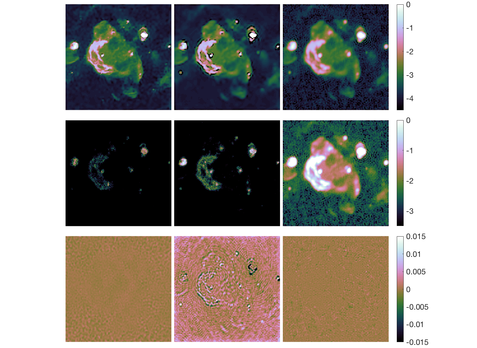
Refer to caption
(b) Channel 60
Refer to caption

Figure 6: Simulations with realistic VLA uυ𝑢𝜐u\upsilon-coverage: reconstruction results obtained by imaging the cube with L=60𝐿60L=60 channels, SR =1absent1=1 and InSNR =60absent60=60 dB. (a) Channel 1, and (b) Channel 60 (the indexing increases with frequency). From left to right, results of the proposed approach HyperSARA (aSNR = 30.13 dB), the monochromatic approach SARA (aSNR = 23.46 dB) and JC-CLEAN (aSNR = 9.39 dB). From top to bottom for (a) and (b) (first and second columns): the estimated model images in log10subscript10\log_{10} scale, the absolute value of the error images in log10subscript10\log_{10} scale and the naturally-weighted residual images in linear scale. From top to bottom for (a) and (b) (third column): the estimated restored images in log10subscript10\log_{10} scale, the absolute value of the error images in log10subscript10\log_{10} scale and the Briggs-weighted residual images in linear scale.

(a) Ground-truth image 𝒙¯0subscript¯𝒙0\bar{\boldsymbol{x}}_{0}
Refer to caption

(b) HyperSARA estimated spectra
Refer to caption

(c) SARA estimated spectra
Refer to caption

(d) JC-CLEAN estimated spectra
Refer to caption

Figure 7: Simulations with realistic VLA uυ𝑢𝜐u\upsilon-coverage: reconstructed spectra of three selected pixels obtained by imaging the cube with L=60𝐿60L=60 channels, SR =1absent1=1 and InSNR =60absent60=60 dB. The results are shown for: (b) the proposed approach HyperSARA, (c) the monochromatic approach SARA and (d) JC-CLEAN, compared with the ground-truth. Each considered pixel is highlighted with a colored circle in the ground-truth image 𝒙¯0subscript¯𝒙0\bar{\boldsymbol{x}}_{0} displayed in (a).

5 Application to real data

In this section, we present the results of HyperSARA for wideband imaging on VLA observations of the radio galaxy Cyg A and the supernova remnant G055.7+3.4121212The considered data sets have been already calibrated with the standard RI pipelines. in comparison with JC-CLEAN (Offringa & Smirnov, 2017) and the single channel image reconstruction algorithm SARA (Carrillo et al., 2012; Dabbech et al., 2018). The latter consists in solving the re-weighted 1subscript1\ell_{1} minimization problem (19) using adaptive PPD algorithm (Dabbech et al., 2018). As opposed to Onose et al. (2017), the 2subscript2\ell_{2} bounds on the data fidelity terms are updated in the algorithm, allowing for imaging in the presence of unknown noise levels and calibration errors. The values of the parameters associated with the adaptive strategy are revealed in Appendix A.

5.1 Data and imaging details

Cyg A:

The data are part of wideband VLA observations within the frequency range 2-18 GHz acquired over two years (2015-2016). We consider here 323232 channels from the S band (2 - 4 GHz) and the C band (4 - 8 GHz) spanning the frequency range 2.045.962.045.962.04-5.96 GHz with a frequency step 128128128 MHz and total bandwidth of 444 GHz (Data courtesy of R.A. Perley). The data in each channel are acquired using the B configuration of the VLA and are of size 25×10425superscript10425\times 10^{4}. We split the data in each channel to 4 blocks of size 6×1046superscript1046\times 10^{4} measurements on average, where each block corresponds to data observed within a time interval over which calibration errors are assumed constant. For imaging, we consider images of size 1024×51210245121024\times 512 with a pixel size δl=0.19𝛿𝑙0.19\delta l=0.19\arcsec. The chosen pixel size corresponds to recovering the signal up to 2.52.52.5 times the nominal resolution at the highest frequency νLsubscript𝜈𝐿\nu_{L}, given by the maximum baseline; BL=max𝒖L,i=1:M𝒖L,i2subscript𝐵𝐿subscriptsubscript𝒖:𝐿𝑖1𝑀subscriptnormsubscript𝒖𝐿𝑖2B_{L}=\max\limits_{\boldsymbol{u}_{L,i=1:M}}\|\boldsymbol{u}_{L,i}\|_{2}131313It is common in RI imaging to set the pixel size δl𝛿𝑙\delta l such that 1/5BLδl1/3BL15subscript𝐵𝐿𝛿𝑙13subscript𝐵𝐿1/5B_{L}\leq\delta l\leq 1/3B_{L}, so that all the PSFs are adequately sampled.. The resulting wideband image cube is of size 1024×512×321024512321024\times 512\times 32. With regards to the choice of the trading-off parameter μ𝜇\mu in HyperSARA, we found that μ^=𝗫dirty/𝚿𝗫dirty2,1^𝜇subscriptnormsuperscript𝗫𝑑𝑖𝑟𝑡𝑦subscriptnormsuperscript𝚿superscript𝗫𝑑𝑖𝑟𝑡𝑦21\hat{\mu}=\|\boldsymbol{\mathsf{X}}^{dirty}\|_{\ast}/\|\boldsymbol{\Psi}^{\dagger}\boldsymbol{\mathsf{X}}^{dirty}\|_{2,1} (as explained in Section 2.3) is large and results in smooth reconstructed model cubes. This can be justified by the fact that the considered data set encompasses calibration errors and the DDEs are not corrected for in our measurement operator. However, we found that setting μ=5×10⁵𝜇5superscript105\mu=5\times 10^{-5} that is two orders of magnitude lower than μ^^𝜇\hat{\mu} is a good trade-off to recover high resolution high dynamic range model cubes. We solve 30 re-weighted minimization problems of the form (5) using the adaptive PPD.

G055.7+3.4:

The data are part of wideband VLA observations at the L band (1 - 2 GHz) acquired in 2010141414Data courtesy of NRAO https://casaguides.nrao.edu/index.php/VLA_CASA_Imaging-CASA5.0.0.. We process 101010 channels from each of the following spectral windows: 1.4441.4981.4441.4981.444-1.498 GHz, 1.7081.7621.7081.7621.708-1.762 GHz and 1.8361.891.8361.891.836-1.89 GHz. Each consecutive 101010 channels, corresponding to one spectral window, have a frequency step of 666 MHz and total bandwidth of 606060 MHz. The data in each channel are of size 4×1054superscript1054\times 10^{5} visibilities, splitted to 4 blocks of size 105superscript10510^{5} measurements on average. The resulting wideband image cube is of size 1280×1280×3012801280301280\times 1280\times 30 with a pixel size δl=8𝛿𝑙8\delta l=8\arcsec. The chosen pixel size corresponds to recovering the signal up to 222 times the nominal resolution of the observations at the highest frequency νLsubscript𝜈𝐿\nu_{L}. In a similar fashion to the Cyg A data set, we fix the trading-off parameter μ𝜇\mu to 5×1065superscript1065\times 10^{-6}. We solve 30 re-weighted minimization problems of the form (5) using the adaptive PPD.

5.2 Imaging quality assessment

To assess the quality of the reconstruction, we perform visual inspection of the obtained images. For HyperSARA and SARA, we consider the estimated model cubes 𝗫^HyperSARAsubscript^𝗫HyperSARA\hat{\boldsymbol{\mathsf{X}}}_{\text{HyperSARA}} and 𝗫^SARAsubscript^𝗫SARA\hat{\boldsymbol{\mathsf{X}}}_{\text{SARA}}, and the naturally-weighted residual image cubes 𝗥HyperSARAsubscript𝗥HyperSARA\boldsymbol{\mathsf{R}}_{\text{HyperSARA}} and 𝗥SARAsubscript𝗥SARA\boldsymbol{\mathsf{R}}_{\text{SARA}}. For JC-CLEAN, we consider Briggs weighting (the robustness parameter is set to 0.50.5-0.5) and examine the resultant restored cube 𝗧^JC-CLEANsubscript^𝗧JC-CLEAN\hat{\boldsymbol{\mathsf{T}}}_{\text{JC-CLEAN}} and the Briggs-weighted residual image cube 𝗥~JC-CLEANsubscript~𝗥JC-CLEAN\tilde{\boldsymbol{\mathsf{R}}}_{\text{JC-CLEAN}}. We report the average standard deviation (aSTD) of all the residual image cubes; aSTD=1/Ll=1LSTDlaSTD1𝐿superscriptsubscript𝑙1𝐿subscriptSTD𝑙\text{aSTD}={1}/{L}\sum_{l=1}^{L}\text{STD}_{l}, where STDlsubscriptSTD𝑙\text{STD}_{l} is the standard deviation of the residual image at the frequency νlsubscript𝜈𝑙\nu_{l}.

We also provide a spectral analysis of selected pixels from the estimated wideband cubes. These are the estimated model cubes 𝗫^HyperSARAsubscript^𝗫HyperSARA\hat{\boldsymbol{\mathsf{X}}}_{\text{HyperSARA}} and 𝗫^SARAsubscript^𝗫SARA\hat{\boldsymbol{\mathsf{X}}}_{\text{SARA}}, and the estimated restored cube 𝗧^JC-CLEANsubscript^𝗧JC-CLEAN\hat{\boldsymbol{\mathsf{T}}}_{\text{JC-CLEAN}}. For the case of unresolved source, i.e. point-like source, we derive its spectra from its total flux at each frequency, integrated over the associated beam area. Finally, we report the similarity of 𝗫^HyperSARAsubscript^𝗫HyperSARA\hat{\boldsymbol{\mathsf{X}}}_{\text{HyperSARA}} and 𝗫^SARAsubscript^𝗫SARA\hat{\boldsymbol{\mathsf{X}}}_{\text{SARA}}. Furthermore, we examine the smoothed versions of 𝗫^HyperSARAsubscript^𝗫HyperSARA\hat{\boldsymbol{\mathsf{X}}}_{\text{HyperSARA}}, 𝗫^SARAsubscript^𝗫SARA\hat{\boldsymbol{\mathsf{X}}}_{\text{SARA}} and 𝗫^JC-CLEANsubscript^𝗫JC-CLEAN\hat{\boldsymbol{\mathsf{X}}}_{\text{JC-CLEAN}} at the resolution of the instrument, denoted by 𝗕^HyperSARAsubscript^𝗕HyperSARA\hat{\boldsymbol{\mathsf{B}}}_{\text{HyperSARA}}, 𝗕^SARAsubscript^𝗕SARA\hat{\boldsymbol{\mathsf{B}}}_{\text{SARA}} and 𝗕^JC-CLEANsubscript^𝗕JC-CLEAN\hat{\boldsymbol{\mathsf{B}}}_{\text{JC-CLEAN}}, respectively. Recall that for channel l𝑙l, 𝒃^l=𝒙^l𝒄lsubscript^𝒃𝑙subscript^𝒙𝑙subscript𝒄𝑙\hat{\boldsymbol{b}}_{l}=\hat{\boldsymbol{x}}_{l}\ast\boldsymbol{c}_{l} where 𝒙^lsubscript^𝒙𝑙\hat{\boldsymbol{x}}_{l} is the estimated model image at the frequency νlsubscript𝜈𝑙\nu_{l} and 𝒄lsubscript𝒄𝑙\boldsymbol{c}_{l} is the respective clean beam. However, we emphasize that smoothing 𝗫^HyperSARAsubscript^𝗫HyperSARA\hat{\boldsymbol{\mathsf{X}}}_{\text{HyperSARA}} and 𝗫^SARAsubscript^𝗫SARA\hat{\boldsymbol{\mathsf{X}}}_{\text{SARA}} is not recommended and is performed here only for comparison purposes with JC-CLEAN.

5.3 Real imaging results

Cyg A:

The estimated images of channels 1 and 32, obtained with the proposed approach HyperSARA, the single channel approach SARA and JC-CLEAN, are displayed in Figure 8. Two key regions in Cyg A are emphasized: these are the hotspots of the east and west jets (second and third columns). We can see that the model images of HyperSARA exhibit more details at the low frequency channels, visible at the hotspots of Cyg A. Moreover, the features of Cyg A at the high frequency channels are better resolved with HyperSARA (see the emission line from the inner core to the east jet and the arc around the right end of the west jet). Imaging quality of the SARA approach is poor at the low frequencies since no inter-channel correlation is exploited and the recovery is limited to the single channel inherent resolution. JC-CLEAN restored images are smooth since they result from convolving the estimated model images with the corresponding clean beams. In Figure 9, we display the naturally-weighted residual images of HyperSARA and SARA. The aSTD values are 1.19×1021.19superscript1021.19\times 10^{-2} and 8.7×1038.7superscript1038.7\times 10^{-3}, respectively which indicates higher fidelity to the naturally-weighted data of the latter. Yet, SARA residual images (right) indicate poor recovery of Cyg A jets at the low frequency channels in comparison with those obtained with HyperSARA (left). Both HyperSARA and SARA residual images present errors at the hotspots pixel positions. These can be justified by calibration errors at those positions. However, larger errors are kept in the residual with HyperSARA and seem to be absorbed in the model images of SARA. HyperSARA and JC-CLEAN Briggs-weighted residual images are shown in Figure 10 with the respective aSTD values are 4.1×1034.1superscript1034.1\times 10^{-3} and 2.1×1032.1superscript1032.1\times 10^{-3}. These indicate higher fidelity of JC-CLEAN to the Briggs-weighted data. Recall that the two approaches solve for two different imaging problems; HyperSARA solves for the naturally-weighted data whereas JC-CLEAN solves for the Briggs-weighted data. Spectral analysis of the different approaches is revealed in Figure 11. One can see that the spectra recovered with HyperSARA have higher intensity values at the low frequency channels, thanks to the re-weighted nuclear norm that enhances the details at the low frequency channels. Finally, given the unknown ground truth, we report the average similarity aSM values of the proposed method with the benchmark approaches. These are aSM(𝗫^HyperSARA,𝗫^SARA)=16.45aSMsubscript^𝗫HyperSARAsubscript^𝗫SARA16.45\text{aSM}(\hat{\boldsymbol{\mathsf{X}}}_{\text{HyperSARA}},\hat{\boldsymbol{\mathsf{X}}}_{\text{SARA}})=16.45 dB while aSM(𝗕^HyperSARA,𝗕^SARA)=36.53aSMsubscript^𝗕HyperSARAsubscript^𝗕SARA36.53\text{aSM}(\hat{\boldsymbol{\mathsf{B}}}_{\text{HyperSARA}},\hat{\boldsymbol{\mathsf{B}}}_{\text{SARA}})=36.53 dB. Also aSM(𝗕^HyperSARA,𝗕^JC-CLEAN)=33.36aSMsubscript^𝗕HyperSARAsubscript^𝗕JC-CLEAN33.36\text{aSM}(\hat{\boldsymbol{\mathsf{B}}}_{\text{HyperSARA}},\hat{\boldsymbol{\mathsf{B}}}_{\text{JC-CLEAN}})=33.36 dB. These values indicate high similarity of the recovered low spatial frequency content with all the methods. In other words, there is strong agreement between the approaches up to the spatial bandwidth of the observations.

(a) Channel 1
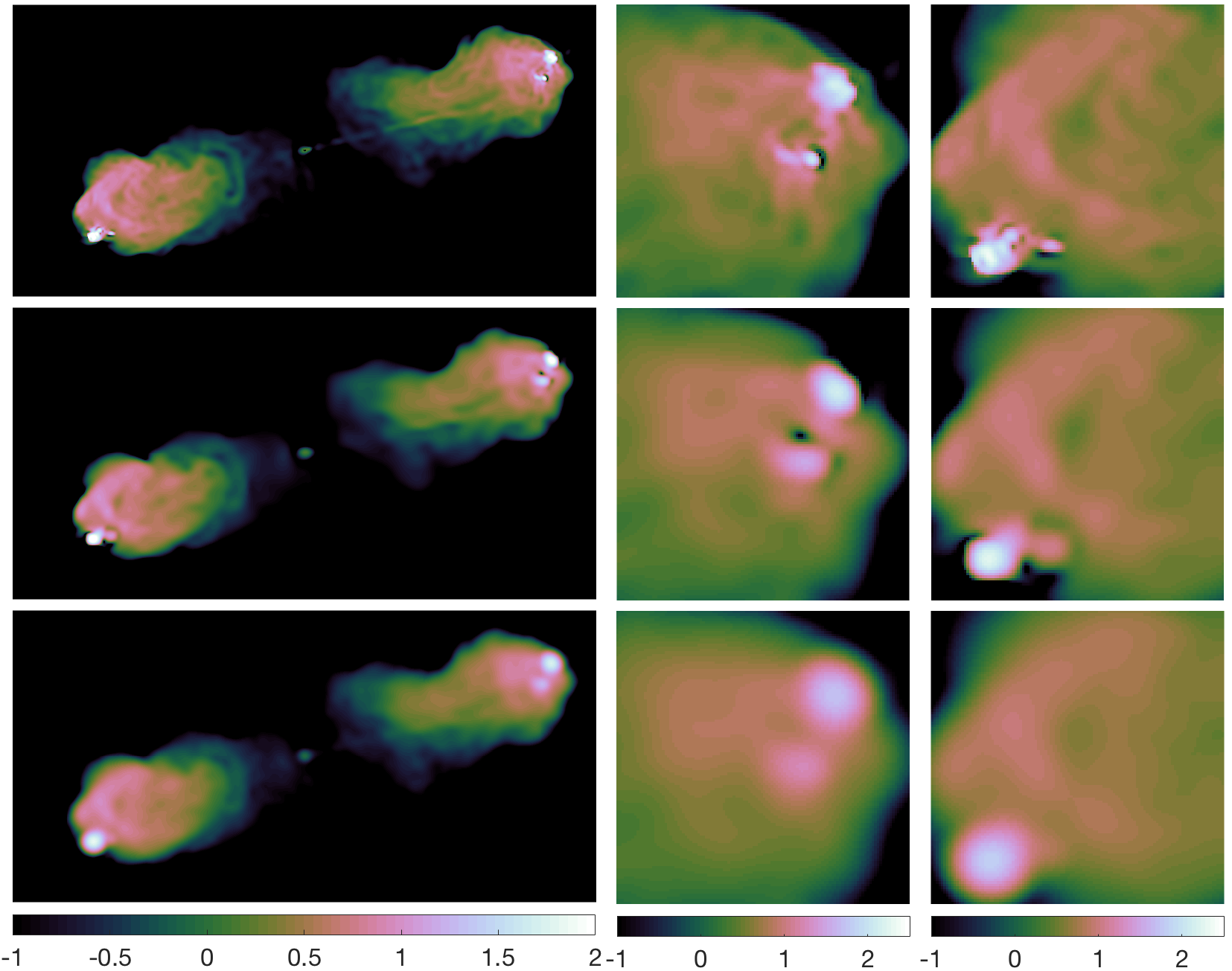
Refer to caption
(b) Channel 32
Refer to caption

Figure 8: Cyg A: recovered images at 2.52.52.5 times the nominal resolution at the highest frequency νLsubscript𝜈𝐿\nu_{L}. (a) Channel 1, and (b) Channel 32 (the indexing increases with frequency). From top to bottom for (a) and (b), estimated model images of the proposed approach HyperSARA, estimated model images of the monochromatic approach SARA and estimated restored images of JC-CLEAN using Briggs weighting. The full images are displayed in log10subscript10\log_{10} scale (first column) as well as zooms on the east jet hotspot (second column) and the west jet hotspot (third column).

(a) Channel 1
Refer to caption
(b) Channel 32
Refer to caption

Figure 9: Cyg A: naturally-weighted residual images obtained by the proposed approach HyperSARA (left) and the monochromatic approach SARA (right). (a) Channel 1, and (b) Channel 32 (the indexing increases with frequency). The aSTD values are 1.19×1021.19superscript1021.19\times 10^{-2} and 8.7×1038.7superscript1038.7\times 10^{-3}, respectively.

(a) Channel 1
Refer to caption
(b) Channel 32
Refer to caption

Figure 10: Cyg A: Briggs-weighted residual images obtained by the proposed approach HyperSARA (left) and JC-CLEAN (right). (a) Channel 1, and (b) Channel 32 (the indexing increases with frequency). The aSTD values are 4.1×1034.1superscript1034.1\times 10^{-3} and 2.1×1032.1superscript1032.1\times 10^{-3}, respectively.

(a) Estimated model image of HyperSARA at channel 323232
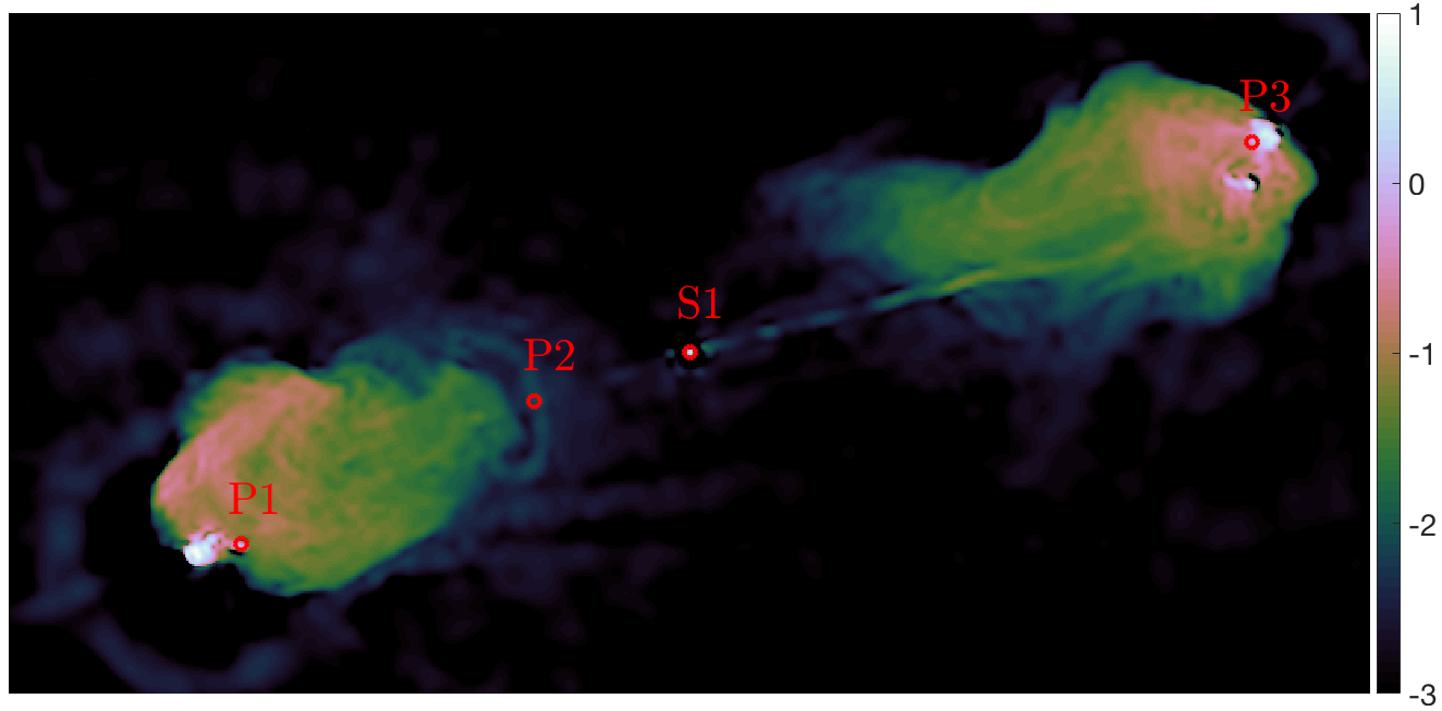
Refer to caption

(b) Selected pixel P1
Refer to caption
(d) Selected source S1
Refer to caption

(c) Selected pixel P2
Refer to caption
(e) Selected pixel P3
Refer to caption

Figure 11: Cyg A: reconstructed spectra of selected pixels and point-like sources obtained by the different approaches. Each considered pixel (P) or source (S) is highlighted with a red circle on the estimated model image of HyperSARA at channel 323232 displayed in (a).

G055.7+3.4:

In Figure 12, we present the reconstructed images of channels 1 and 30, obtained with the proposed approach HyperSARA, the single channel approach SARA and JC-CLEAN. The figures clearly demonstrate a significantly higher performance of HyperSARA in terms of resolution and dynamic range. For instance, one can see that the central extended emission is very well captured by HyperSARA in the overall estimated model cube as opposed to SARA and JC-CLEAN. While SARA presents a smooth representation of the source, JC-CLEAN provides a highly noisy representation. Moreover, the number of modelled point sources is clearly higher with HyperSARA in particular at the low channels unlike SARA where only few sources are detected whereas JC-CLEAN present a large number of false detections. This suggests the efficiency of the HyperSARA priors in capturing the correlation of the data cube and enhancing the dynamic range of the recovered model cube. The naturally-weighted residual images of HyperSARA and SARA are shown in Figure 13. The aSTD values are 6.55×1056.55superscript1056.55\times 10^{-5} and 8.37×1058.37superscript1058.37\times 10^{-5}, respectively, which reflects the higher fidelity to data achieved by HyperSARA. The Briggs-weighted residual images of HyperSARA and JC-CLEAN are also displayed in Figure 14, their respective aSTD values are 1.12×1041.12superscript1041.12\times 10^{-4} and 7.75×1057.75superscript1057.75\times 10^{-5}. These indicate higher fidelity of JC-CLEAN to the Briggs-weighted data. Finally, we show examples of the recovered spectra with the different approaches in Figure 15. When inspecting the different spectra, one can see that HyperSARA succeeds to recover the scrutinized sources with higher flux in comparison with the other approaches. Finally, we report the average similarity values of the proposed method with the benchmark approaches. These are aSM(𝗫^HyperSARA,𝗫^SARA)=9.13aSMsubscript^𝗫HyperSARAsubscript^𝗫SARA9.13\text{aSM}(\hat{\boldsymbol{\mathsf{X}}}_{\text{HyperSARA}},\hat{\boldsymbol{\mathsf{X}}}_{\text{SARA}})=9.13 dB while aSM(𝗕^HyperSARA,𝗕^SARA)=12.3aSMsubscript^𝗕HyperSARAsubscript^𝗕SARA12.3\text{aSM}(\hat{\boldsymbol{\mathsf{B}}}_{\text{HyperSARA}},\hat{\boldsymbol{\mathsf{B}}}_{\text{SARA}})=12.3 dB. Also aSM(𝗕^HyperSARA,𝗕^JC-CLEAN)=7.1aSMsubscript^𝗕HyperSARAsubscript^𝗕JC-CLEAN7.1\text{aSM}(\hat{\boldsymbol{\mathsf{B}}}_{\text{HyperSARA}},\hat{\boldsymbol{\mathsf{B}}}_{\text{JC-CLEAN}})=7.1 dB. The low aSM values confirm the large disagreement in the quality of the recovery up to the resolution of the instrument, that is in agreement with the visual inspection of the estimated images.

(a) Channel 1
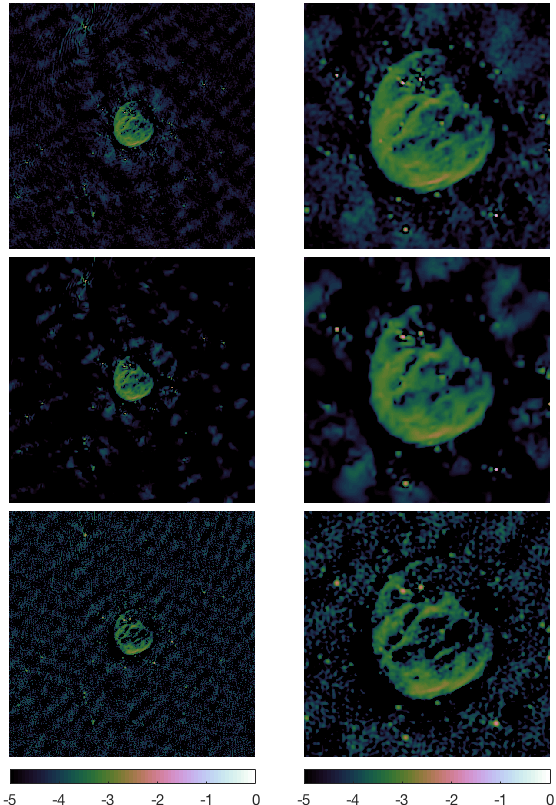
Refer to caption

(b) Channel 30
Refer to caption

Figure 12: G055.7+3.4: recovered images at 222 times the nominal resolution at the highest frequency νLsubscript𝜈𝐿\nu_{L} . (a) Channel 1, and (b) Channel 30 (the indexing increases with frequency). From top to bottom for (a) and (b), estimated model images of the proposed approach HyperSARA, estimated model images of the monochromatic approach SARA and estimated restored images of JC-CLEAN using Briggs weighting. The full images are displayed in log10subscript10\log_{10} scale (first column) as well as zoom on the central region (second column).

(a) Channel 1
Refer to caption
(b) Channel 30
Refer to caption

Figure 13: G055.7+3.4: naturally-weighted residual images obtained by the proposed approach HyperSARA (left) and the monochromatic approach SARA (right). (a) Channel 1, and (b) Channel 30 (the indexing increases with frequency). The aSTD values are 6.55×1056.55superscript1056.55\times 10^{-5} and 8.37×1058.37superscript1058.37\times 10^{-5}, respectively.

(a) Channel 1
Refer to caption
(b) Channel 30
Refer to caption

Figure 14: G055.7+3.4: Briggs-weighted residual images obtained by the proposed approach HyperSARA (left) and JC-CLEAN (right). (a) Channel 1, and (b) Channel 30 (the indexing increases with frequency). The aSTD values are 1.12×1041.12superscript1041.12\times 10^{-4} and 7.75×1057.75superscript1057.75\times 10^{-5}, respectively.

(a) Estimated model image of HyperSARA at channel 303030
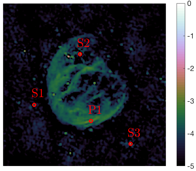
Refer to caption

(b) Selected source S1
Refer to caption
(d) Selected pixel P1
Refer to caption

(c) Selected source S2
Refer to caption
(e) Selected source S3
Refer to caption

Figure 15: G055.7+3.4: reconstructed spectra of selected pixels and point-like sources obtained by the different approaches. Each considered pixel (P) or source (S) is highlighted with a red circle on the estimated model image of HyperSARA at channel 303030 (first row).

6 Conclusions

In this paper, we presented the HyperSARA approach for wideband RI image reconstruction. It consists in solving a sequence of weighted nuclear norm and 2,1subscript21\ell_{2,1} minimization problems to better approximate low rankness and joint average sparsity in 0subscript0\ell_{0} sense. HyperSARA is able to achieve higher resolution of the reconstructed wideband model cube thanks to the re-weighted nuclear norm that enforces inter-channel correlation. The overall dynamic range is also enhanced thanks to the re-weighted 2,1subscript21\ell_{2,1} norm that rejects decorrelated artefacts present on the different channels. The efficiency of HyperSARA was validated on simulations and VLA observations in comparison with the single channel imaging approach SARA and the clean-based wideband imaging algorithm JC-CLEAN. As opposed to the clean-based methods, the sophisticated priors of HyperSARA come at the expense of increased computational cost and memory requirements. To mitigate this effect, we adopt the primal-dual algorithmic structure defined in the context of the theory of convex optimization, owing to its highly interesting functionalities for wideband RI imaging. We have leveraged the preconditioning functionality to provide accelerated convergence. The functionality of parallelization of the different functions and operators involved in the minimization task was also promoted as a way to spread the computational cost and memory requirements due to the large data volumes over a multitude of processing nodes with limited resources. Establishing the full scalablity potential of our approach is the matter of ongoing research. Our matlab code is available online on github, https://github.com/basp-group/Puri-Psi/. We intend to provide an efficient c++ implementation of HyperSARA with a distributed computing infrastructure.

Acknowledgements

The authors warmly thank R.A. Perley (NRAO, USA) for providing the VLA observations of the Cyg A galaxy and also for the enriching discussions. The National Radio Astronomy Observatory is a facility of the National Science Foundation operated under cooperative agreement by Associated Universities, Inc. This work was supported by the UK Engineering and Physical Sciences Research Council (EPSRC, grants EP/M011089/1 and EP/M008843/1) and used the Cirrus UK National Tier-2 HPC Service at EPCC (http://www.cirrus.ac.uk) funded by the University of Edinburgh and EPSRC (EP/P020267/1).

References

  • Abdulaziz et al. (2016) Abdulaziz A., Dabbech A., Onose A., Wiaux Y., 2016, in 2016 24th European Signal Processing Conference (EUSIPCO). pp 388–392
  • Abdulaziz et al. (2017) Abdulaziz A., Onose A., Dabbech A., Wiaux Y., 2017, in International Biomedical and Astronomical Signal Processing Frontiers Workshop. p. 6
  • Ammanouil et al. (2017) Ammanouil R., Ferrari A., Flamary R., Ferrari C., Mary D., 2017, in 2017 25th European Signal Processing Conference (EUSIPCO). pp 1435–1439
  • Bauschke & Combettes (2011) Bauschke H. H., Combettes P. L., 2011, Convex analysis and monotone operator theory in Hilbert spaces. Springer Science & Business Media
  • Bhatnagar & Cornwell (2004) Bhatnagar S., Cornwell T., 2004, Astronomy & Astrophysics, 426, 747
  • Brogan et al. (2006) Brogan C. L., Gelfand J., Gaensler B., Kassim N., Lazio T., 2006, The Astrophysical Journal Letters, 639, L25
  • Carrillo et al. (2012) Carrillo R. E., McEwen J. D., Wiaux Y., 2012, Monthly Notices of the Royal Astronomical Society, 426, 1223
  • Carrillo et al. (2014) Carrillo R. E., McEwen J. D., Wiaux Y., 2014, Monthly Notices of the Royal Astronomical Society, 439, 3591
  • Clark (1980) Clark B., 1980, Astronomy and Astrophysics, 89, 377
  • Combettes & Vũ (2014) Combettes P. L., Vũ B. C., 2014, Optimization, 63, 1289
  • Condat (2013) Condat L., 2013, Journal of Optimization Theory and Applications, 158, 460
  • Cornwell (2008) Cornwell T. J., 2008, IEEE Journal of Selected Topics in Signal Processing, 2, 793
  • Dabbech et al. (2012) Dabbech A., Mary D., Ferrari C., 2012, in 2012 IEEE International Conference on Acoustics, Speech and Signal Processing (ICASSP). pp 3665–3668
  • Dabbech et al. (2015) Dabbech A., Ferrari C., Mary D., Slezak E., Smirnov O., Kenyon J. S., 2015, Astronomy and Astrophysics, 576, 16
  • Dabbech et al. (2018) Dabbech A., Onose A., Abdulaziz A., Perley R. A., Smirnov O. M., Wiaux Y., 2018, Monthly Notices of the Royal Astronomical Society, 476, 2853
  • Deguignet et al. (2016) Deguignet J., Ferrari A., Mary D., Ferrari C., 2016, in 2016 24th European Signal Processing Conference (EUSIPCO). pp 1483–1487
  • Dewdney et al. (2013) Dewdney P., Turner W., Millenaar R., McCool R., Lazio J., Cornwell T., 2013, Document number SKA-TEL-SKO-DD-001 Revision, 1
  • Ferrari et al. (2015) Ferrari A., Deguignet J., Ferrari C., Mary D., Schutz A., Smirnov O., 2015, arXiv preprint arXiv:1504.06847
  • Garsden et al. (2015) Garsden H., et al., 2015, Astronomy & astrophysics, 575, A90
  • Girard et al. (2015) Girard J., Garsden H., Starck J., Corbel S., Woiselle A., Tasse C., McKean J., Bobin J., 2015, Journal of Instrumentation, 10, C08013
  • Golbabaee & Vandergheynst (2012) Golbabaee M., Vandergheynst P., 2012, in 2012 IEEE International Conference on Acoustics, Speech and Signal Processing (ICASSP). pp 2741–2744
  • Hiriart-Urruty & Lemaréchal (1993) Hiriart-Urruty J.-B., Lemaréchal C., 1993, Convex analysis and minimization algorithms II: Advanced theory and bundle methods, vol. 306 of Grundlehren der mathematischen Wissenschaften
  • Högbom (1974) Högbom J., 1974, Astronomy and Astrophysics Supplement Series, 15, 417
  • Jiang et al. (2017) Jiang M., Bobin J., Starck J., 2017, SIAM Journal on Imaging Sciences, 10, 1997
  • Johnson et al. (2017) Johnson M. D., et al., 2017, The Astrophysical Journal, 850, 172
  • Junklewitz et al. (2015) Junklewitz H., Bell M. R., Enßlin T., 2015, Astronomy & Astrophysics, 581, A59
  • Junklewitz et al. (2016) Junklewitz H., Bell M., Selig M., Enßlin T., 2016, Astronomy & Astrophysics, 586, A76
  • Koopmans et al. (2015) Koopmans L., et al., 2015, arXiv preprint arXiv:1505.07568
  • Li, F. et al. (2011) Li, F. Cornwell, T. J. de Hoog, F. 2011, Astronomy & Astrophysics, 528, A31
  • Melanie et al. (2014) Melanie J., et al., 2014, Proceedings of Science, 9-13-June-2014
  • Moreau (1965) Moreau J.-J., 1965, Bulletin de la Société mathématique de France, 93, 273
  • Offringa & Smirnov (2017) Offringa A., Smirnov O., 2017, Monthly Notices of the Royal Astronomical Society, 471, 301
  • Offringa et al. (2014) Offringa A., et al., 2014, Monthly Notices of the Royal Astronomical Society, 444, 606
  • Onose et al. (2016a) Onose A., Carrillo R. E., McEwen J. D., Wiaux Y., 2016a, in 2016 24th European Signal Processing Conference (EUSIPCO). pp 1448–1452
  • Onose et al. (2016b) Onose A., Carrillo R. E., Repetti A., McEwen J. D., Thiran J.-P., Pesquet J.-C., Wiaux Y., 2016b, Monthly Notices of the Royal Astronomical Society, 462, 4314
  • Onose et al. (2017) Onose A., Dabbech A., Wiaux Y., 2017, Monthly Notices of the Royal Astronomical Society, 469, 938
  • Perley et al. (2011) Perley R., Chandler C., Butler B., Wrobel J., 2011, The Astrophysical Journal Letters, 739, L1
  • Pesquet & Repetti (2014) Pesquet J.-C., Repetti A., 2014, arXiv preprint arXiv:1406.6404
  • Pratley et al. (2017) Pratley L., McEwen J. D., d’Avezac M., Carrillo R. E., Onose A., Wiaux Y., 2017, Monthly Notices of the Royal Astronomical Society, 473, 1038
  • Rau & Cornwell (2011) Rau U., Cornwell T. J., 2011, Astronomy & Astrophysics, 532, A71
  • Rybicki & Lightman (2008) Rybicki G. B., Lightman A. P., 2008, Radiative processes in astrophysics. John Wiley & Sons
  • Sault & Wieringa (1994) Sault R., Wieringa M., 1994, Astronomy and Astrophysics Supplement Series, 108
  • Schwab & Cotton (1983) Schwab F. R., Cotton W. D., 1983, The Astronomical Journal, 88, 688
  • Thompson et al. (2007) Thompson A. R., Moran J. M., Swenson G. W., 2007, Interferometry and Synthesis in Radio Astronomy. Wiley-VCH
  • Van Haarlem et al. (2013) Van Haarlem M., et al., 2013, Astronomy & Astrophysics, 556, A2
  • Vũ (2013) Vũ B. C., 2013, Advances in Computational Mathematics, 38, 667
  • Wenger & Magnor (2014) Wenger S., Magnor M., 2014, Technical report, A sparse reconstruction algorithm for multi-frequency radio images. Computer Graphics Lab, TU Braunschweig
  • Wenger et al. (2010) Wenger S., Magnor M., Pihlström Y., Bhatnagar S., Rau U., 2010, Publications of the Astronomical Society of the Pacific, 122, 1367
  • Wiaux et al. (2009) Wiaux Y., Jacques L., Puy G., Scaife A. M. M., Vandergheynst P., 2009, Monthly Notices of the Royal Astronomical Society, 395, 1733

Appendix A Overview of the parameters specific to Adaptive PPD

An overview of the variables and parameters involved in the adjustment of the 2subscript2\ell_{2} bounds on the data fidelity terms is presented in Tables 1 and 2, respectively.

Table 1: Overview of the variables employed in the adaptive procedure incorporated in Algorithm 2.
ρlb(t)superscriptsuperscriptsubscript𝜌𝑙𝑏𝑡{\rho_{l}^{b}}^{(t)} the 2subscript2\ell_{2} norm of the residual data corresponding to the data block 𝒚lbsuperscriptsubscript𝒚𝑙𝑏\boldsymbol{y}_{l}^{b} at iteration t𝑡t.
ϑlb(t1)superscriptsuperscriptsubscriptitalic-ϑ𝑙𝑏𝑡1{\vartheta_{l}^{b}}^{(t-1)} iteration index of the previous update of the 2subscript2\ell_{2} bound of the data block 𝒚lbsuperscriptsubscript𝒚𝑙𝑏\boldsymbol{y}_{l}^{b}.
β(t1)superscript𝛽𝑡1\beta^{(t-1)} the relative variation of the solution at iteration t1𝑡1t-1.
Table 2: Overview of the parameters involved in the adaptive procedure incorporated in Algorithm 2.
λ1]0,1[\lambda_{1}\in]0,~{}1[ the bound on the relative variation of the solution (we fix it to 5×1045superscript1045\times 10^{-4}).
λ2]0,1[\lambda_{2}\in]0,~{}1[ the tolerance on the relative difference between the current estimate of a data block 2subscript2\ell_{2} bound and the 2subscript2\ell_{2} norm of the associated residual data (we fix it to 0.01).
λ3]0,1[\lambda_{3}\in]0,~{}1[ the parameter defining the increment of the 2subscript2\ell_{2} bound with respect to the 2subscript2\ell_{2} norm of the residual data (we fix it to 0.618).
ϑ¯¯italic-ϑ\bar{\vartheta} the minimum number of iterations between consecutive updates of each 2subscript2\ell_{2} bound (we fix it to 100).