Learning in Integer Latent Variable Models
with Nested Automatic Differentiation
Abstract
We develop nested automatic differentiation (AD) algorithms for exact inference and learning in integer latent variable models. Recently, Winner, Sujono, and Sheldon showed how to reduce marginalization in a class of integer latent variable models to evaluating a probability generating function which contains many levels of nested high-order derivatives. We contribute faster and more stable AD algorithms for this challenging problem and a novel algorithm to compute exact gradients for learning. These contributions lead to significantly faster and more accurate learning algorithms, and are the first AD algorithms whose running time is polynomial in the number of levels of nesting.
1 Introduction
In a recent line of work, Winner & Sheldon (2016) and Winner et al. (2017) developed the first exact inference algorithms for a class of hidden Markov models (HMMs) with integer latent variables. Such models are used to model populations that change over time in ecology or epidemiology (Dail & Madsen, 2011; Heathcote, 1965). Standard inference techniques do not apply to these models because marginalization would require summing over the infinite support of the latent variables. Instead, they showed how to reformulate the forward algorithm for HMMs to use probability generating functions (PGFs) as its internal representation of probability distributions and messages. These PGFs can be represented compactly and encode all the information about the infinite-support distributions. Inference tasks such as computing the likelihood are reduced to evaluating PGFs and their derivatives.
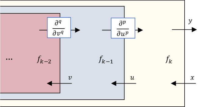
However, the PGFs are complex functions that are defined recursively in terms of high-order derivatives of other PGFs. Figure 1 illustrates such a function. The function , on input , first computes a value , then computes the th derivative of with respect to , and then uses the result to compute its own output value . The function itself involves nested derivatives of , and so on, with total levels of nesting. The goal is to compute the function , and possibly derivatives thereof. It is natural to consider automatic differentiation (AD) techniques for this task. However, this is a very difficult setting for AD. There are many levels of nesting and the total order of differentation may number in the hundreds or thousands.
In this paper we subtantially improve AD algorithms for inference in integer latent variable models, and develop new AD algorithms to support learning. For inference, we conceptually simplify the AD techniques of (Winner et al., 2017) and root them more firmly in the AD literature. We show that nested derivatives of univariate functions can be handled by an extension to the basic AD computation model that allows nested derivative nodes, which are just derivatives of another function defined by a computation graph (e.g., the “node” in Figure 1). The AD algorithm needs only a thin adapter to handle the change of scope between the inner and outer functions. For the inference application, this places nearly all of the complexity in the general-purpose AD toolkit and simplifies the application.
We also make substantial stability and speed improvements to the AD algorithms. We show that implementing core AD operations using the logarithmic number system (LNS) to accurately represent signed real numbers with high dynamic range allows the algorithms to scale to very high order derivatives—something which is not possible with a standard floating point representation. We also adopt fast power series composition for core AD operations (Brent & Kung, 1978), which are asympotically faster than those used in (Winner et al., 2017).
Finally, we contribute new AD algorithms to compute exact gradients of the log-likelihood in integer HMMs by extending (higher-order) forward-over-reverse AD to handle nested derivatives. This allows us to compute gradients of functions like the one in Figure 1, where is a vector of parameters for the entire nested computation. We show experimentally that our new LNS-based AD algorithms are the only inference algorithms for integer latent variable models that are simultaneously accurate, fast, and stable, and that our novel algorithms for computing exact gradients lead to significantly faster and more accurate parameter estimation.
2 Model and Problem Statement
We consider the integer hidden Markov model (HMM) from (Winner et al., 2017), an HMM with integer latent variables representing a population that changes over time through the processes of immigration, reproduction, and mortality, and which is partially observed at each time step. The model is:
| (1) | ||||
| (2) |
with the initial condition . The variable is the population size at the th time step, and is the observed number, assuming that each indvidual is observed with probability . The population size depends on an offspring process and an immigration process. First, each individual present at time contributes individuals to the present time step, where are iid random variables from the offspring distribution. The “offspring” of one individual can include (or not include) itself, immediate offspring, or descendants of more than one generation, depending on the choices of the modeler. In particular, this distribution is used to model both survival and reproduction. Additionally, individuals enter the population, where is drawn from the immigration distribution. The offspring and immigration distributions can be arbitrary count-valued distributions, and will be specified through their PGFs as described below.
Problem Statement.
The application goal is usually to estimate a parameter vector controlling the offspring and immigration distributions given some number of observations of this process (Dail & Madsen, 2011). We will focus on computing the log-likelihood and its gradient, which together will enable optimization routines to find maximum likelihood estimates. Let be the total number of time steps and let (similar notation will be used throughout the paper). Our goal is to compute and .
Inference via PGFs.
Standard HMM inference algorithms such as the forward algorithm (Rabiner, 1989) do not apply here because the latent variables are unbounded. Hence, the messages have infinite length, and marginalization of any variable involves an infinite sum. Winner & Sheldon (2016) and Winner et al. (2017) showed how the forward algorithm can be reformulated to use PGFs to represent messages. Standard inference tasks, such as computing the likelihood, are then converted to the problem of evaluating recursively-defined PGFs.
Definition 1.
The PGF of a (not necessarily normalized) probability distribution is the power series with probability values as coefficients.
To formulate the forward algorithm using PGFs, define and . These are the “messages” that are recursively computed within the standard forward algorithm. The PGFs of and are defined (using the corresponding capital letters) as and . The utility of switching to a PGF representation is summarized in the following proposition.
Proposition 1 (Winner & Sheldon 2016; Winner et al. 2017).
Let and be the PGFs for the offspring and immigration distributions, respectively. The PGFs and satisfy the following recurrence:
| (3) | ||||
| (4) |
with the base case . The likelihood can be recovered from the final PGFs as .
Equation (3) follows from the model definition and standard manipulations of PGFs, and is well known in the literature on branching processes (Heathcote, 1965). Equation (4) may appear surprising. It includes the th derivative of the function from Equation (3). The derivatives are related to the selection of particular terms in the joint PGF of and corresponding to the observed value of .
Proposition 1 gives a recipe to compute the exact log-likelihood and its gradient. We need to compute and , where is defined in terms of the prior PGFs through Equations (3) and (4), and we have introduced the parameter vector , which includes the detection probabilities and any parameters of and . Despite the somewhat complex appearance of the recurrence, it implies a well-defined feed-forward computation to calculate from the constituent functions , and . The key complication is the fact that this function contains deeply nested high-order derivatives: calls , which calls , which calls , and so on. Winner et al. (2017) developed a method based on automatic differentation to efficiently compute , which we will extend in this paper to be more robust and efficient, and to compute gradients.
3 Autodiff Approach
Our problem is to compute and for the function , which includes nested high-order derivatives. To set up the proper recursion we will generalize this to the following:
| Problem 1: compute and |
Now we will abstract away from the particular from the previous section and consider any defined according to a particular computation model, where will be called the input and the vector will be called the parameters. We will first describe how to solve both parts of Problem 1 in a basic computation model, and then extend the model to handle nested derivatives.
3.1 Computation Model and Dual Numbers
The basic computation model for is shown in Algorithm 1, following (Griewank & Walther, 2008). In Line 3, the function is a primitive operation that operates on the variables , where is the set of predecessors of , and is the subvector of corresponding to index set . The predecessor relationship defines the computation graph , a directed acyclic graph (DAG) with edges from to for all .
Partial computations and dual numbers. We wish to express derivatives of a variable with respect to a preceding variable . To make this precise, for , we denote the partial computation from to as . This is defined as the function that maps from fixed values of to the value of obtained by executing the procedure above starting with the assignment to and ending with the assignment to . A formal recurrence for is given in the supplement. We can now define precisely the derivative of with respect to :
Definition 2.
For , a generalized dual number is the sequence of derivatives of with respect to up to order :
We say that is a dual number of order with respect to . We will commonly write dual numbers as:
in which case it is understood that and for some , and will be clear from context.
This definition generalizes standard (higher-order) dual numbers by explicitly tracking the variable with respect to which we differentiate. In standard forward-mode autodiff, this would always be . The generalization is important for nested differentation, where we will instantiate intermediate dual numbers with respect to different variables.
Remark 1 (Dual numbers as Taylor series coefficients).
A dual number can be viewed as holding Taylor series coefficients. In particular, the dual number encodes the first coefficients of the Taylor series of about :
Most forward AD methods store and propagate dual numbers as truncated Taylor series (Griewank & Walther, 2008; Pearlmutter & Siskind, 2007).
3.2 Higher-Order Forward Mode
We now discuss how to solve the first part of Problem 1—computing in the basic computation model—using forward AD. Higher-order forward mode works by propagating dual numbers instead of real numbers through the computation. For this to work, each local computation must be “lifted” to accept dual numbers as inputs and to output a dual number.
Definition 3 (Lifted Function).
Let be a function of variables . The lifted function is the function that accepts as input dual numbers and returns the dual number .
We defer the details of how a function is lifted for the moment. If we are able to lift each primitive operation in the original procedure, we can execute it using dual numbers (with respect to ) in place of real numbers. The procedure is shown in Algorithm 2. The output is a dual number with respect to , from which we can extract the derivatives for . Note that in Line 2, we did not write the parameter values as dual numbers; we will allow in our notation a real number to be used as an input to a lifted operation , with the understanding that: (1) does not depend on , and (2) will be promoted to the dual number .
It is well known how to lift basic mathematical operations:
Proposition 2 (Griewank & Walther 2008).
The arithmetic operations , , , , viewed as functions of and , and the mathematical functions , , , can be lifted to operate on dual numbers of order . In each case, the lifted function runs in time.
As a result, forward-mode autodiff can compute the first derivatives of any function that uses only these primitive operations in time times the running time of .
3.3 Forward-Over-Reverse AD
For the purpose of learning, we need to solve the second part of Problem 1 and compute the gradient This can be accomplished using “forward-over-reverse” AD, which is based on the relatively simple observation that we can switch the order of differentation to see that
which reveals that what we want is also the higher-order derivative of with respect to . The well-known reverse mode of autodiff (or backpropagation) provides a procedure to compute . Then, by executing reverse mode using dual numbers instead of real numbers, we can obtain . Forward-over-reverse AD is shown in Algorithm 3. It incrementally computes the adjoint:
for all in a reverse sweep through the computation graph. The final adjoint values are dual numbers, from which the derivatives with respect to of the parameter gradients can be extracted. As in the forward mode, we need to lift the primitive operations of the procedure. In this case the primitive operations are those that compute the partial derivatives of with respect to its own inputs. When is a simple mathematical operation (, , , , , , etc.), these partial derivatives are also simple and can be lifted by standard techniques (cf. Proposition 2).
3.4 Forward Mode with Nested Derivatives
We now extend the forward AD algorithms to handle nested derivatives within the computation procedure. For the most part, we use ideas that were present in (Winner et al., 2017). However, we simplify the conceptual framework considerably, so that all we need to do is lift a function that takes the derivative of another function, which leads to a conceptual improvement of the AD techniques and a dramatic simplification of the inference application.
Extended computation model: nested derivative nodes. Although the functions are usually conceptualized as simple “primitive” operations, they may be arbitrarily complex as long as we know how to lift them—i.e., modify them to propagate dual numbers. So, assume now that one or more of the functions is a nested derivative node, which takes the derivative of some other function with respect to one of its inputs:
| (5) |
Here we consider to be “parameters” of the nested computation. We need to reason about how to lift to propagate dual numbers with respect to . We will make the following restriction on , with which we can reason about the sensitivity of to through alone:
Assumption 1.
There is no path in from to .
Lifting a univariate primitive via composition of Taylor series. We wish to lift a nested derivative node . To do so, we will discuss the general procedure to lift a univariate function . We may temporarily suppress the parameters from notation because they are constant with respect to . Here is the general setting. We have completed the partial computation to compute the first derivatives of with respect to . We wish to compute the first derivatives of . This can be done by composing the Taylor series of and .
Proposition 3.
Suppose and are analytic. Let be the Taylor series expansion of about , and let be the Taylor series expansion of about . Then the Taylor series expansion of about is:
The first coefficients of in encode the first derivatives of , and can be computed by power series composition algorithms from the first coefficients of the power series and .
Proposition 3 (proved in the supplement) is the foundation of higher-order forward mode. The input to is the dual number , which gives us the first coefficients of , i.e., . The function is typically a simple mathematical primitive (e.g., ), which will have a very special Taylor series . The goal is to compute the first coefficients of . In most cases of “true” primitive operations, specialized routines exist to do this in or time (Griewank & Walther, 2008; Brent & Kung, 1978). For general , Brent & Kung (1978) describe fast algorithms to compute the first coefficients of from the first coefficients of and . The compose operation we implement will run in time—see Section 4.
Algorithm 4 shows the Compose operation for two dual numbers and , which extracts Taylor coefficients from the dual numbers and then performs power series composition to compute .
Lifting a nested derivative node. We now return to the specifics of lifting a nested derivative node to propagate dual numbers with respect to (we temporarily drop subscripts without ambiguity). Note that the semantics of the partial differentiation operation would be simple if we were propagating dual numbers with respect to : we would just shift all derivatives in the sequence lower by positions (see the Diff operator in Algorithm 5). So, our solution to nested derivatives will be to temporarily instantiate a new dual number with respect to within the scope of , propagate this through to compute the derivatives of with respect to , apply the Diff operator to the result, and then apply the Compose operation to convert back to a dual number with respect to . The whole procedure is detailed in Algorithm 6.
By using this procedure to lift nested derivative nodes, we can now run forward AD in the extended computation model. Furthermore, because we lift the nested function by recursively applying forward AD to it, we can handle recursively nested derivatives (of univariate functions, i.e., subject to Assumption 1). One can prove inductively that the running time increases by a modest factor, regardless of the number of levels of nested derivatives. Specifically, let be the maximum order of differentiation, which, for a nested derivative node, is equal to its own order plus that of the calling procedure. In the lifted procedure, each operation takes times its original running time, where is the maximum time of an operation on dual numbers of order , which in our models is the Compose operation.
Proposition 4.
Higher-order forward AD can be extended to handle nested univariate derivatives by recursively calling forward AD using Algorithm 6. The running time is bounded by times the number of primitive operations, where is the maximum order of differentiation, and is the time to compose two power series of order .
3.5 Nested Forward-Over-Reverse
We now wish to extend forward-over-reverse AD to the computation model in which can be a nested derivative node. By examining Algorithm 3, we see in Line 4 that we will need to lift a function of the form . By again switching the order of differentiation, the function to be lifted is:
where is the scalar-valued function that computes the partial derivative of with respect to . Observe that this is just another nested derivative node—for the function that computes the partial derivative of —which we can lift using Algorithm 6. In practice, we don’t need to apply Algorithm 6 separately for each partial derivative. We can compute for all simultaneously by (recursively) applying forward-over-reverse AD to , within a procedure similar to Algorithm 6 (details omitted). This will be more efficient because it only needs one forward and reverse sweep through the computation graph for . In summary:
Proposition 5.
Forward-over-reverse AD can also be extended to handle nested derivative nodes by recursively calling forward-over-reverse AD using Algorithm 6 (or a more efficient variant). The running time is times that of the original computation.
4 Application and Implementation
We now return to inference and learning in integer HMMs. The log-likelihood (Equation 3) clearly fits within the extended computation model: it involves only basic mathematical primitives and a nested derivative of . Therefore, we can apply the nested forward-over-reverse AD algorithms from Section 3 to compute the log-likelihood and its gradient. Observe that the total number of levels of nesting is and the maximum order of differentiation is .
This is a unique application of AD. The total order may number in the hundreds or thousands with ten or more levels of nesting. For comparison, typical values of , even in high-order applications, are single digits (Griewank & Walther, 2008). Applications of nested AD are rare; reported examples involve only one level of nesting (Siskind & Pearlmutter, 2008; Foo et al., 2008; Maclaurin et al., 2015; Domke, 2012). Because of the very high order and nesting, we faced significant implementation challenges related to two interrelated issues: numerical stability and asymptotic efficiency of power series operations. We describe in this section the steps needed to overcome these.
4.1 Numerical Stability: Logarithmic Number System
The core computations in our approach are lifted primitive operations for dual numbers (Proposition 2), and the Compose operation. Both operate on Taylor series coefficients of the form for from to . Due to the factor in each coefficient and the fact that the derivatives themselves may have high dynamic range, overflow and underflow are significant problems and unavoidable for greater than a few hundred if coefficients are stored directly in floating point. Such problems are familiar in probabilistic inference, where a standard solution is to log transform all values and use stable operations such as logsumexp whenever this transformation needs to be undone.
Our solution is similar, but more difficult for several reasons. To see why, it is helpful to see the nature of algorithms to lift primitive operations, which use convolutions or related recurrences (Griewank & Walther, 2008). As an example, here is the recurrence for the division operation to compute the Taylor coefficients of the function given the Taylor coefficients of :
Observe that we must handle subtraction and negative values, unlike standard probabilistic inference. Also, both multiplication and addition are required in the innermost loop of the algorithm (the right hand side includes multiplication and addition of the most recently computed value ) so it is not possible to batch multiplications and additions, with transformation to and from log-space only between batches.
Our solution, which generalizes the “log-space trick” for probabilistic inference, is to store coefficients using a logarithmic number system (LNS, Swartzlander & Alexopoulos 1975), and implement core power series operations in LNS. In LNS, a real number is represented as where is the sign bit and is the log of the magnitude of , stored in fixed precision. The multiplication, division, and power operations are simple and efficient in LNS, while addition and subtraction require more effort. For example, if and are both positive, then . We implemented LNS in C using a floating-point instead of fixed point internal representation to interface more easily with existing mathematical functions. Addition and subtraction use the C standard library’s log1p function, and are much more expensive than floating point operations, despite the fact they are, in principle, single “arithmetic operations”, and could be comparable to floating point operations with appropriate hardware (Coleman et al., 2000).
4.2 Fast and Accurate Power Series Operations
The lifting procedures for primitive operations that we describe above all take time and have recurrences that resemble convolutions. Multiplication can be done in time using FFT-based convolution, and algorithms for most other primitives can be also be derived using the FFT (Brent & Kung, 1978). Although our application certainly reaches the regime where FFT is faster than direct convolution, existing FFT implementations require that we transform coefficients out of LNS into floating point, which led to inaccurate results and numerical problems when we tried this. Similar observations have been made in previous applications of FFT for probabilistic inference (Wilson & Keich, 2016). A possible future remedy is to implement the FFT in LNS (Swartzlander et al., 1983), however, our current implementation uses the direct algorithms.
The Compose operation is a bottleneck and should be implemented as efficiently as possible. Winner et al. (2017) used a naive composition algorithm. Brent & Kung (1978) present two fast algorithms—BK 2.1 and BK 2.2—for power series composition. BK 2.2 has the fastest known running time of with FFT convolution, but may be slower in practice (Johansson, 2015) and we have already ruled out FFT convolution. Instead, we use BK 2.1, which, in our setting, runs in time and achieves substantial speedups over the naive algorithm.
5 Experiments
We conducted experiments on the accuracy, speed, and stability of AD inference algorithms for integer HMMs, and of parameter estimation using AD gradient algorithms.
Inference: Accuracy, Speed, Stability. We evaluated four methods for inference in integer HMMs. Trunc and Trunc-FFT are variants of a truncated forward algorithm, which is currently used in practice in ecological applications (Dail & Madsen, 2011). These place an a priori upper bound on the values of the hidden variables and then apply the standard forward algorithm for discrete HMMs. They require a convolution of the offspring and immigration distributions to compute the transition probabilities (details are given in the supplement), and take time with direct convolution and time with FFT convolution. They can be implemented in log-space easily, but FFT convolutions must be done in linear space, which can lead to accuracy loss (Wilson & Keich, 2016). Selecting in the truncated algorithms is a challenge. A too-small value will cut off some of the probability mass and lead to the wrong result, and a too-large value will lead to high running time. For these experiments, we iteratively doubled until the log-likelihood converged (to a precision of 5 decimal places) or until reached an absolute limit of 2500, and only measured the running time of the final iteration. Note that this is a conservative comparison that hides the cost of tuning this value in practice.
The AD and AD-LNS methods use nested AD to compute , with the latter storing coefficients in LNS. With our conceptual simplification of nested AD, these algorithms are now nearly a direct translation of Equations (3) and (4), with all of work done by the AD routines. We show the full 15-line Python implementation in the supplementary material. AD and AD-LNS both have running time, where .
 |
 |
 |
 |
| Bernoulli offspring | Poisson offspring |
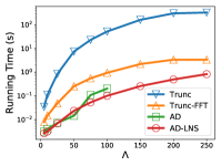
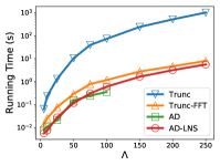
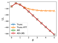
We generated data from integer HMMs, performed inference with each algorithm, and compared the resulting values and running times. In Figure 2, top, we scaled the population size by generating data with immigration distribution for increasing , and fixed offspring distributions or . Here, controls the immigration rate, and the expectation of all variables scales in proportion to , as do the parameters and controlling the running time of the algorithms. We ran inference using the true parameters. The plots show running time on a log scale. AD and AD-LNS are the fastest algorithms, but AD is unstable (due to overflow) and does not compute a result for . Trunc-FFT is somewhat slower than the AD algorithms. AD-LNS is especially fast for Bernoulli offspring because the Bernoulli PGF is linear, which leads to many zero power series coefficients, and LNS addition of zero is a very fast special case. The Poisson results should be considered the general case.
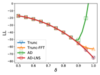
Figure 2, bottom, compares the accuracy of different methods. Here, we generated data from a model with , immigration for , and offspring distributions and with . We performed inference for different values of . This simulates the situation encountered during estimation when an optimizer queries the log-likelihood at an unlikely parameter setting; it is important that the methods are robust in this case. We see that as increases from the true value of , Trunc-FFT (in both models) and AD (in Bernoulli) deviate from the correct answer. This is likely due to loss of numerical precision in floating point operations, either in the FFT algorithm or in power series algorithms.
Overall, AD-LNS is the only one of the four inference algorithms that is fast, stable (does not overflow or underflow), and accurate over a wide range of parameter settings.
 |
 |
| Single parameter | parameters |
 |
 |
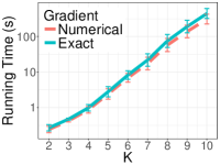
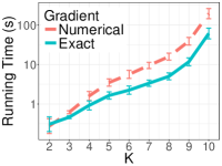
Learning: Speed and Accuracy. We now evaluate the speed and accuracy of learning. We generate data from an integer HMM and use the L-BFGS (Liu & Nocedal, 1989) algorithm to recover parameters by maximizing the log-likelihood. Based on the inference results, we consider as a baseline the optimizer that uses AD-LNS to compute the likelihood and numerically estimates gradients by finite differences. The per-iteration cost to compute numerical gradients is the number of parameters times the cost to compute the log-likelihood (or twice this if central differences are used). For our approach, we used nested forward-over-reverse AD algorithm to compute exact gradients. In this case, the running time to compute the gradient is a constant factor greater than the time to compute the log-likelihood. We predict based on this that as the number of parameters increases, exact gradients will be faster.
Figure 3 shows the results. For each trial, we simulate 20 independent realizations of the integer HMM for up to time steps, with immigration distribution and . For the left plot, the offspring distribution is not time-varying, and we fit only the single parameter . In this case, the cost of numerical gradient is only twice that of computing the objective, and the two methods behave similarly. Note that the running time is shown on a log scale. In the right plot, the offspring distribution is time-varying, with , and we fit each of these values for a total of parameters. In this case, we see that the exact gradient method is several times faster for . The running time of both methods increases with due to the increased cost of inference. We saw similar results across a wide range of models, and expect the benefits of using exact gradients to be even more significant for models with more parameters.
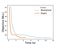
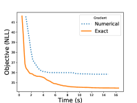
In most cases, the optimizer followed nearly the exact same sequence of parameter values regardless of the gradient computation, but was faster with exact gradients; in some cases the algorithm with exact gradients took more iterations and achieved a better objective value. See Figure 4.
6 Discussion
We introduce new AD techniques for inference in integer HMMs. By cleanly incorporating nested derivatives into the AD computation model, we greatly simplify the algorithms for inference using PGFs. By implementing forward-mode AD operations using the logarithmic number system and using fast power series algorithms, we achieve fast, accurate, and stable algorithms for very high-order derivatives. Our new techniques for nested forward-over-reverse AD allow us to compute exact gradients in integer HMMs for the first time, which leads to significantly faster, and sometimes more accurate, learning procedures.
Related work. An alternate approach to compute nested derivatives is to repeatedly apply AD at each level of nesting starting with the innermost, for example, using source transformation. Pearlmutter & Siskind (2007) and Siskind & Pearlmutter (2008) introduced a tagging mechanism for forward AD to properly handle nesting and avoid “perturbation confusion” (Siskind & Pearlmutter, 2005); this idea is impemented in functional AD tools such as DiffSharp (Baydin et al., 2015). However, since each application of AD increases running time by a constant factor, and the innermost function is “transformed” each time (either through source transformation or by adding a new tagged perturbation), the running time of these approaches is exponential in the number of levels of nesting, while our running time is polynomial. But note that these methods can handle more general functions than ours (i.e., multivariate, not subject to Assumption 1). An interesting avenue of future work is to extend our approach to multivariate nested derivatives.
Acknowledgments
This material is based upon work supported by the National Science Foundation under Grants No. 1617533 and 1522054.
References
- Baydin et al. (2015) Baydin, A. G., Pearlmutter, B. A., Radul, A. A., and Siskind, J. M. Automatic differentiation in machine learning: a survey. arXiv preprint arXiv:1502.05767, 2015.
- Brent & Kung (1978) Brent, R. P. and Kung, H. T. Fast algorithms for manipulating formal power series. Journal of the ACM (JACM), 25(4):581–595, 1978.
- Coleman et al. (2000) Coleman, J. N., Chester, E. I., Softley, C. I., and Kadlec, J. Arithmetic on the European logarithmic microprocessor. IEEE Transactions on Computers, 49(7):702–715, 2000.
- Dail & Madsen (2011) Dail, D. and Madsen, L. Models for estimating abundance from repeated counts of an open metapopulation. Biometrics, 67(2):577–587, 2011.
- Domke (2012) Domke, J. Generic methods for optimization-based modeling. In Artificial Intelligence and Statistics, pp. 318–326, 2012.
- Foo et al. (2008) Foo, C.-s., Do, C. B., and Ng, A. Y. Efficient multiple hyperparameter learning for log-linear models. In Advances in neural information processing systems, pp. 377–384, 2008.
- Griewank & Walther (2008) Griewank, A. and Walther, A. Evaluating derivatives: principles and techniques of algorithmic differentiation. SIAM, 2008.
- Heathcote (1965) Heathcote, C. R. A branching process allowing immigration. Journal of the Royal Statistical Society. Series B (Methodological), 27(1):138–143, 1965.
- Johansson (2015) Johansson, F. A fast algorithm for reversion of power series. Mathematics of Computation, 84(291):475–484, 2015.
- Liu & Nocedal (1989) Liu, D. C. and Nocedal, J. On the limited memory BFGS method for large scale optimization. Math. Program., 45(3):503–528, December 1989.
- Maclaurin et al. (2015) Maclaurin, D., Duvenaud, D., and Adams, R. Gradient-based hyperparameter optimization through reversible learning. In International Conference on Machine Learning (ICML), pp. 2113–2122, 2015.
- Pearlmutter & Siskind (2007) Pearlmutter, B. A. and Siskind, J. M. Lazy multivariate higher-order forward-mode AD. In Symposium on Principles of Programming Languages (POPL), pp. 155–160, 2007.
- Rabiner (1989) Rabiner, L. A tutorial on hidden Markov models and selected applications in speech recognition. Proceedings of the IEEE, 77(2):257–286, 1989.
- Siskind & Pearlmutter (2005) Siskind, J. M. and Pearlmutter, B. A. Perturbation confusion and referential transparency: Correct functional implementation of forward-mode AD. 2005.
- Siskind & Pearlmutter (2008) Siskind, J. M. and Pearlmutter, B. A. Nesting forward-mode AD in a functional framework. Higher-Order and Symbolic Computation, 21(4):361–376, Dec 2008.
- Swartzlander & Alexopoulos (1975) Swartzlander, E. E. and Alexopoulos, A. G. The sign/logarithm number system. IEEE Transactions on Computers, 100(12):1238–1242, 1975.
- Swartzlander et al. (1983) Swartzlander, E. E. J., Chandra, D. V. S., Nagle, H. T. J., and Starks, S. A. Sign/logarithm arithmetic for FFT implementation. IEEE Transactions on Computers, C-32(6):526–534, 1983.
- Wilson & Keich (2016) Wilson, H. and Keich, U. Accurate pairwise convolutions of non-negative vectors via FFT. Computational Statistics and Data Analysis, 101:300–315, 2016.
- Winner & Sheldon (2016) Winner, K. and Sheldon, D. Probabilistic inference with generating functions for Poisson latent variable models. In Advances in Neural Information Processing Systems 29, 2016.
- Winner et al. (2017) Winner, K., Sujono, D., and Sheldon, D. Exact inference for integer latent-variable models. In International Conference on Machine Learning (ICML), pp. 3761–3770, 2017.
Appendix A Definition of Partial Computation
Formally, we can write , the partial computation from to , via the recurrence:
Here, will equal for all . For , the value is obtained directly from the inputs to . For , the value of is computed according to the partial computation from to .
Appendix B Proof of Proposition 3
Proof.
We write as a function of using the two given Taylor expansions:
where we used the Taylor expansion of in Line 3 and the Taylor expansion of in Line 4. The last expression is a power series in , and, since is analytic (the composition of two analytic functions is analytic), it is necessarily the Taylor series expansion of about . ∎
Appendix C Truncated Forward Algorithm
The truncated forward algorithm is the following variant of the forward algorithm for discrete HMMs, where is an upper bound placed on the population size:
-
1.
Set and for to .
-
2.
For to
-
(a)
Compute the transition matrix , where for all (details below)
-
(b)
For to , set
-
(a)
-
3.
The likelihood is
Step 2(b) takes time. Step 2(a) may take or time, depending on how it is implemented. Observe that is the sum of two random variables:
and we must reason about their convolution to construct the transition probabilities. Specifically, the th row of is the convolution of the first values of the distribution and the first values of :
Let us assume we can compute the first values of each distribution in time. Then the time to compute each row of is if we use the direct convolution formula above, but if we use the fast Fourier transform (FFT) for convolution, making the overall procedure either or . While the FFT is superior in terms of running time, it is inaccurate in many cases (see Section 5).